Embed Size (px)
Citation preview

VIDEO-GUIDED AUTONOMOUS
POLLINATOR ROTORCRAFT
TUNG X. DAO
GRADUATE STUDENT OF AEROSPACE ENGINEERING
SAN JOSE STATE UNIVERSITY
SAN JOSE, CA 95192
A MASTER PROJECT PRESENTED TO
DR. NIKOS J. MOURTOS, DR. SEAN SWEI,
AND PROF. GONZALO MENDOZA
MAY 2013

The Designated Master Project Committee Approves the Master Project Titled
VIDEO-GUIDED AUTONOMOUS
POLLINATOR ROTORCRAFT
By
Tung X. Dao
Approved for the Department of Aerospace Engineering
San Jose State University
May 2013
Dr. Nikos J. Mourtos, Committee Chair Date
Dr. Sean Swei, Committee Member Date
Prof. Gonzalo Mendoza, Committee Member Date

3
Table of Contents
I. Introduction and problem statement ........................................................................................................... 4 II. Current research ......................................................................................................................................... 4 III. Literature search ......................................................................................................................................... 4
A. Pollination of Flowers .............................................................................................................................. 5 B. Image processing background and methods ............................................................................................ 5
IV. Available devices ....................................................................................................................................... 7 V. Proposed solution ....................................................................................................................................... 8
A. Project Scope ........................................................................................................................................... 8 B. Timeline and project deliverables ............................................................................................................ 8
VI. Image Recognition Programs and Hardware ............................................................................................. 9 A. OpenCV ................................................................................................................................................... 9 B. Cameras ................................................................................................................................................... 9
VII. Image Recognition Testing ...................................................................................................................... 10 A. Cascade Classifiers ................................................................................................................................ 10 B. Controls ................................................................................................................................................. 11 C. Ranging .................................................................................................................................................. 11 D. CMUcam4 ............................................................................................................................................. 13
VIII. Navigation and Automation: Initial High-Level Algorithms ................................................................... 14 A. Mission/Flight Profile ............................................................................................................................ 14 B. Navigation model ................................................................................................................................... 14 C. Automation model ................................................................................................................................. 14 D. Traveling Salesman Problem ................................................................................................................. 15
IX. Systems Testing Plan ............................................................................................................................... 15 A. Flight platform ....................................................................................................................................... 15 B. 0-D model .............................................................................................................................................. 15 C. 1-D model .............................................................................................................................................. 15 D. 2-D model .............................................................................................................................................. 15 E. 3-D model .............................................................................................................................................. 16
X. Arduino Development .............................................................................................................................. 16 A. Servo control with Arduino ................................................................................................................... 16 B. Input/output ........................................................................................................................................... 16 C. Libraries and Functions ......................................................................................................................... 17 D. SparkFun MPU-6050 Inertial Measurement Unit .................................................................................. 17 E. Code Segments ...................................................................................................................................... 18
XI. Parameter Identification ........................................................................................................................... 25 A. Quadrotor System Identification ............................................................................................................ 26 B. CMUcam4 parameter ID ....................................................................................................................... 34
XII. Flight platform flight tests........................................................................................................................ 35 A. Preliminary flight tests ........................................................................................................................... 35
XIII. Future work .............................................................................................................................................. 36 XIV. Conclusion ............................................................................................................................................... 37 Appendix A – Cost Breakdown ............................................................................................................................. 38 Appendix B ............................................................................................................................................................ 38 Appendix C ............................................................................................................................................................ 39 Appendix D ............................................................................................................................................................ 42 Appendix E – NAVFIT results for Pitch, Yaw, and Throttle ................................................................................. 43 Acknowledgements ................................................................................................................................................ 45 Bibliography .......................................................................................................................................................... 45
4
Video-Guided Autonomous Pollinator Rotorcraft
Tung X. Dao
San Jose State University, San Jose, CA 95192
This paper details the design of a video-guided autonomous pollinator rotorcraft. The
literature search reveals that a large body of research and similar projects provide the
necessary information to realize the final product. The project achieved basic control
through image recognition with the CMUcam4 and Arduino system. Further development
includes parameter identification of the quadrotor and preliminary design of simple
autonomous control routines.
I. Introduction and problem statement
umans use bee colonies to pollinate key agricultural crops and to provide honey worldwide. However, the bee
population has been suffering from colony collapse disorder in recent years, which have reduced the number of
bees available for pollination. Factors such as poor weather, pesticide use, diseases, varroa mites, and mono-crop
diets have contributed to the decline in bee population [1]. The decline in the pollinator population causes serious
problems for humans. Bees pollinate key crops including apples, oranges, avocados, and almonds [2]. The disap-
pearance of bees can mean higher prices or the disappearance of these foods. Additionally, colony prices have
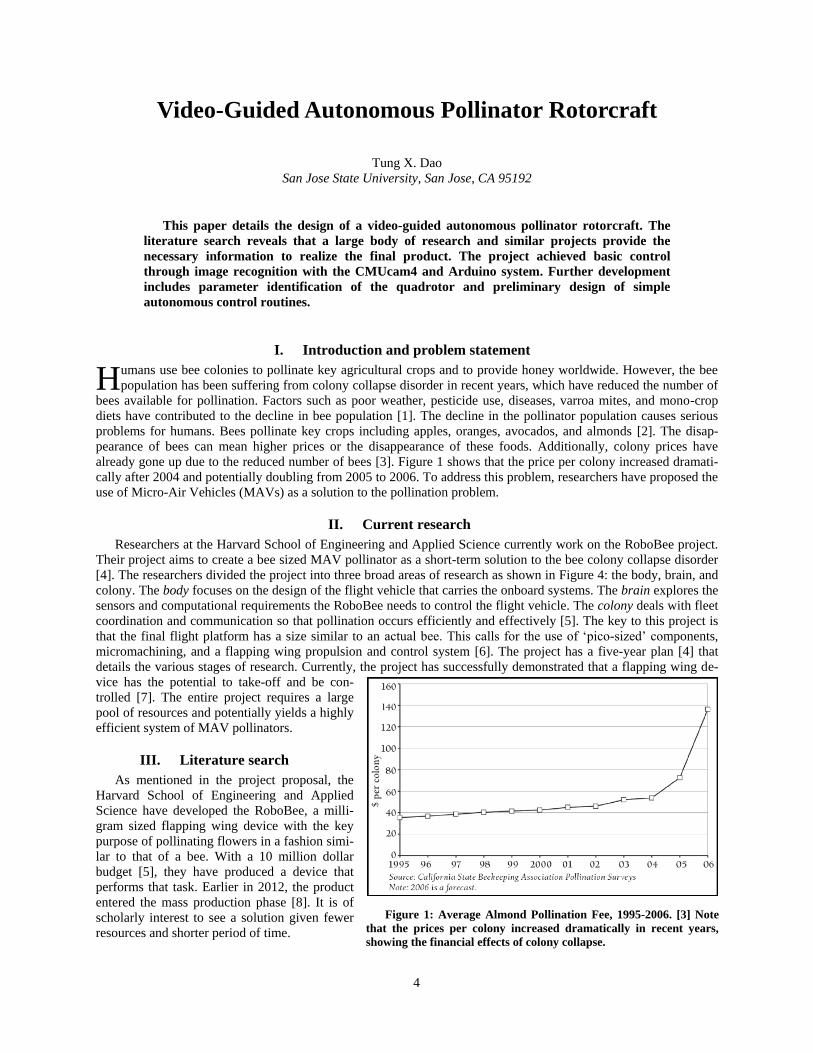
already gone up due to the reduced number of bees [3]. Figure 1 shows that the price per colony increased dramati-
cally after 2004 and potentially doubling from 2005 to 2006. To address this problem, researchers have proposed the
use of Micro-Air Vehicles (MAVs) as a solution to the pollination problem.
II. Current research
Researchers at the Harvard School of Engineering and Applied Science currently work on the RoboBee project.
Their project aims to create a bee sized MAV pollinator as a short-term solution to the bee colony collapse disorder
[4]. The researchers divided the project into three broad areas of research as shown in Figure 4: the body, brain, and
colony. The body focuses on the design of the flight vehicle that carries the onboard systems. The brain explores the
sensors and computational requirements the RoboBee needs to control the flight vehicle. The colony deals with fleet
coordination and communication so that pollination occurs efficiently and effectively [5]. The key to this project is
that the final flight platform has a size similar to an actual bee. This calls for the use of ‘pico-sized’ components,
micromachining, and a flapping wing propulsion and control system [6]. The project has a five-year plan [4] that
details the various stages of research. Currently, the project has successfully demonstrated that a flapping wing de-
vice has the potential to take-off and be con-
trolled [7]. The entire project requires a large
pool of resources and potentially yields a highly
efficient system of MAV pollinators.
III. Literature search
As mentioned in the project proposal, the
Harvard School of Engineering and Applied
Science have developed the RoboBee, a milli-
gram sized flapping wing device with the key
purpose of pollinating flowers in a fashion simi-
lar to that of a bee. With a 10 million dollar
budget [5], they have produced a device that
performs that task. Earlier in 2012, the product
entered the mass production phase [8]. It is of
scholarly interest to see a solution given fewer
resources and shorter period of time.
H
Figure 1: Average Almond Pollination Fee, 1995-2006. [3] Note
that the prices per colony increased dramatically in recent years,
showing the financial effects of colony collapse.

Video-Guided Autonomous Pollinator Rotorcraft
5
Another test platform that utilizes a video
feed for guidance is AVATAR (Autonomous
Vehicle Aerial Tracking and Reconnais-
sance). The device has a PC-104 stack, a
GPS, an antenna for wireless communica-
tion, a Boeing CMIGTS-II inertial navigation
system, and 3 axis accelerometers and gyro-
scopes [9]. The camera functions as an aid to
the classical navigation hardware when GPS
does not exist and the fact that GPS does not
allow for object detection and avoidance [9].
This demonstrates that the combination of a
camera with a set of traditional sensors plays
a crucial role in adding autonomy to a ro-
torcraft. Most importantly, it allows the flight
platform to approach a target in ways that
classical navigation sensors cannot.
In the field of model aircraft, FPV (First
Person View) flying consists of mounting a camera onto a radio controlled flight vehicle with a wireless transmitter
[10]. The wireless transmitter sends the video-feed back to a ground station where a pilot can control the flight vehi-
cle based on the information sent back by the feed. This system requires a pilot to control the aircraft, which does
not satisfy the mission requirements for this project. However, it does show that flight vehicles with onboard camer-
as exist, and that the components are available for purchase, if necessary.
A. Pollination of Flowers
Early assumptions modeled successful tagging as successful contact of the probe to the center of the flower. Ad-
ditional research verifies this assumption and clarifies the actual biological requirements for successful pollination.
The method of transfer for a plant varies depending on the crop, but can vary from birds, insects, wind, and self-
pollination [11] [12]. In a general sense, pollination occurs when pollen is transferred from the anther (male) to the
pistil (female) [11] [13]. This requires that the probe is capable of transferring pollen to the pistil after coming into
contact with the anther. Some plants produce separate flowers that contain the anther or the pistil [11]. This then
requires the probe to carry pollen from one flower to another flower. The high-level algorithm assumes that both
male and female flowers will be visited by random selection during the pollination process. Thus the initial assump-
tion that contact with the center of the flower yields successful pollen transfer is established, especially for the
purposes of flight-testing.
The flight platform will use a simple visible spectrum for the purposes of testing. Flowers provide a visual cue
that attracts animals to come and pollinate the flowers. Bees and insects see patterns in the UV spectrum that human
cannot see without technological aids [14] [12]. It is also possible to use visible light imaging for the production
model if the crop produces flowers with a distinctive color from the surrounding foliage. The shapes that the image
recognition algorithm needs to detect can range from a simple dark circle [12] to more complex patterns [14]. The
algorithm needs to be fine-tuned to know these patterns a priori for each flower. The test pattern will have a pattern
that is representative of a flower.
B. Image processing background and methods
Another application of image recognition exists in the field of social media. Facial recognition systems also exist
and have implementation in the photographic field. For example, cameras such as the Canon 7D and many others
have facial detection algorithms that detect faces. The onboard processor then uses these faces as reference points
for the autofocus system to control the focus onto these areas of heightened interest. By doing so, the camera can aid
the photographer in selecting important image features to focus on. In online social media, facial recognition helps
users tag photographs that have their friends in them. From these examples, it is clear that image recognition is not
impossible, especially when computers can determine features such as faces. Thus, some methods must exist for
recognizing faces. The concept can then be further applied to recognizing flowers. The following section discusses
various methods used in image recognition in aerospace applications.
1. Visual odometer
By using two cameras, researcher Omead Amidi developed a method for determining the distance between a hel-
icopter and an object [15]. The principle is based upon the parallax between two offset cameras. He also developed
Figure 2: (a) An ordinary-light image of a flower. (b) An example of
how a bee sees a flower [12]. Note that the pattern is only visible with
UV imaging. However, also note that the flower stands out from the
background with its bright color in (a). This can allow visible light im-
aging for guidance.

Video-Guided Autonomous Pollinator Rotorcraft
6
algorithms for object tracking and vehicle positioning using the con-
cepts of optical flow, target image scaling, rotation, and
normalization [15]. The text also contains an overview of vector
math and coordinate transforms involved with positioning and veloc-
ity determination based on the optical flow.
2. Kalman filter
Many different platforms use the Kalman filter in its systems to
predict motion and provide image tracking based on the information
from a camera presented in a visual field [16] [17] [18]. Two systems
that use the Kalman filter are AVATAR (which has a 16 state
Kalman filter), and COLIBRI (which uses a Kalman filter in its flight
computer) [16]. Since incoming signals from any source has random
noise in it, a means is necessary to estimate the actual state from the
noisy data. The Kalman filter can be used to implement a predictor-
corrector estimator that minimizes the estimated error covariance of
the data [17]. This results in an estimation of the actual state that can
be used to command the flight platform. In one instance, the output
from the Kalman filter can be used to control velocity and other low-
er level commands such as heading and attitude [16]. Lower level
commands include simple stabilizing actions for pitch and roll [19].
See the section on Autonomy for more information on behavior based autonomy.
An Extended Kalman Filter (EKF) can be used when the stochastic difference equation is no longer linear.
Wantabe used an EKF “so that it can be applied to nonlinear systems by linearizing the system about the predicted
estimate at each time step” [20]. MATLAB currently has a Kalman filter function available that outputs the result of
the Kalman filter estimations.
3. Color blobs
When computational power imposes a constraint, color blobs can provide a simple means of target identification.
The CMUcam4 shield has this algorithm built in. The algorithm looks for pixels with color coordinates within a
predefined color range in the RGB or YUV color space [21]. The data can then be used to generate a centroid loca-
tion that represents the center of the target and a confidence level that represents how certain the image processor
believes the centroid belongs to the target [22]. Until the project requires more advanced image recognition, this
method may be sufficient to provide the target position data to navigate the flight platform.
4. Invariant moments
Invariant moments form the foundation for one method used to determine if an object resembles a previously
known object. The method uses properties of a shape that are invariant to scale, rotation, and translation to deter-
mine the object’s orientation relative to the camera. Features such as perimeter, area, and moments carry sufficient
information to enable a computer to perform object recognition [9] [16]. Saripelli uses the area moments to deter-
mine the orientation of a helipad to guide the helicopter towards the target. This method can be used to fulfill the
same task of tagging a target. However, invariant moments do not tell us if the object is rotated about an axis per-
pendicular to the line of sight between the object and camera. It may be possible to have a database of invariant
moments for flowers at different angles for the algorithm to compare against, and compute another piece of infor-
mation from a 2-D image.
5. Lucas-Kanade algorithm
Once an object has been identified, its current position needs to be tracked. The Lucas-Kanade algorithm per-
forms this task by minimizing the sum of squared error between two successive images [16]. Similar to the Kalman
filter, this algorithm uses the optical flow estimation based on the apparent 2-D velocity to estimate where the object
of interest will appear in the next time step. The outputs from the filter can be used to estimate the velocity vector
for a tracked object “by averaging the optical flow within the object’s bounding box” [18].
6. SLAM
Flight platforms flying in unknown territory can build a virtual map of the area by using Simultaneous Localiza-
tion and Mapping (SLAM) [23]. This concept can become very important when addressing automation in the
pollination problem. The flight platform may need to build up a virtual map of all target positions to determine the
optimum path to cover all targets. Alternatively, it can be used to remember previously encountered targets and
avoid retagging inefficiencies.
Figure 3: Saripelli’s landing algorithm shows
the process which the helicopter goes through
to land using a camera guided system [9].

Video-Guided Autonomous Pollinator Rotorcraft
7
7. SIFT
David Lowe developed the Scale Invariant
Feature Transform (SIFT) in 1999 [24] [25]. It
offers robust object recognition in cluttered and
partially-occluded images [25]. This feature is
important since the targets in the pollination prob-
lem exist in a visually noisy environment that
includes leaves and other distractions. The object
recognition system needs to be able to determine
the object’s location in such an environment,
which the SIFT method may prove useful.
8. Other methods
a. Foveal Vision
Foveal vision utilizes two cameras to simulate
the way the human eye works during image
recognition and tracking. Gould et al. uses two
cameras to accomplish this task: a high-resolution
camera recognizes objects and a low-resolution
camera that tracks objects [18]. Since the mass
and computational budget may be very demand-
ing in this particular application, this method may
not be as suitable at first glance.
b. Interest Model
Lastly, there exists an interest model developed by Gould et al. for the rapid identification of unknown pixels
that are likely to be of interest [18].
9. Autonomy
Autonomy utilizes a set of algorithms of simple routines that build on one another out of which complex behav-
ior emerges. One example of an autonomous behavior can be seen in Figure 3. The algorithm shows the order of
events depending on the current state of the system. The rules show what a self-organizing behavior can look like.
This is important, as the vision system may not always have a lock on the target. For the autonomous pollinator,
Saripelli’s algorithm can form a basic structure for the tagging algorithm. On the aircraft level, Saripelli implements
a different algorithm called behavior based control shown in Figure 5 that allows the helicopter to perform the ma-
neuvers required by this high level landing algorithm. The lower level behaviors include reflex behaviors that
stabilize the helicopter. Above that are the higher level commands that guide the helicopter through longer term
commands. By combining the different levels of control,
Saripelli can create the behavior needed to land a helicopter.
This model has value in building the algorithm for the pollina-
tor.
IV. Available devices
The current market has a wide array of tools available that
can be used together to create a virtual or physical model for
the pollinator. The Arduino ArduPilot system provides open-
source software and premade hardware components that allow
anyone to build a rotorcraft or aircraft to a wide variety of mis-
sion specifications. However, a control system can be built
from the ground up with a microprocessor board such as the
Arduino Uno or Mega. Initial research shows that MATLAB
may be able to handle the SIFT algorithm, and can definitely
handle the Kalman filter, video, object detection, and tracking.
Video cameras such as the CMUcam4 also exist that can be
connected to a controller board or a laptop to allow for com-
puter vision.
Figure 4: The research team at the Harvard School of Engi-
neering and Applied Sciences divides the research into three
areas of study: body, brain, and colony [5]. The research special-
ties of the team members are listed within each sub-discipline
within the three major divisions.
Figure 5: Saripelli’s behavior based control has
multiple levels of control that build on each other to
allow the helicopter to land itself with a
camera [9].
Video-Guided Autonomous Pollinator Rotorcraft
8
V. Proposed solution
Instead of creating a highly specialized and efficient centimeter-sized pollinator over a long span of time, a dif-
ferent approach can yield a less efficient, but still functional, final product. The author proposes to convert a fully
functional remotely piloted rotorcraft into a fully automated flying device that finds targets and navigates itself. Cur-
rently, a live video guidance system may suit the sensory needs, but further research and analysis will determine the
method. This method makes sense due to the complex 3-D structure of a flowering tree.
The general mission requirement has three parts. First, the rotorcraft needs to demonstrate autonomous take off,
cruise to a predetermined location, and return to base. This simple requirement demonstrates the control system’s
ability to guide the rotorcraft. Second, the rotorcraft needs to mimic the pollinating action like that of a bee. This
places a requirement for some level of precision on the video guidance system. Lastly, the rotorcraft needs to find
flower analogues in a tree-like environment or demonstrate the action with actual trees in an outdoors environment.
This requires some basic level of artificial intelligence. Ideally, this project has a time span of one academic year.
This approach places emphasis on the control system. Since developing a micro-sized flying apparatus from
scratch would pose great difficulty on available resources and such a device already exists, it appears sensible to
focus the video guided controls system only.
A. Project Scope
With the bee colony collapse disorder problem described in the project proposal, the project scope has been fur-
ther refined to meet the time and resource requirements expected to complete the project within the next semester.
The scope now focuses on guidance using visual information gathered from an onboard camera.
The project has three major goals. The first goal is to develop a system that recognizes and tracks objects from a
video feed. The computer, either a laptop or a microcontroller, needs to be able take the output from an onboard
video camera, identify potential targets, extract information about the position of the target relative to the camera,
and then output a control command for the flight controller. The flight controller would then use this information to
guide the rotorcraft. The second goal is to navigate the rotorcraft towards the target, tag it, and then fly back. This
requires a set of control laws or an algorithm that commands the flight platform throughout the different stages of
flight. The algorithm can include phases such as search, approach, slow-down, tag, retreat, and repeat. The last goal
is to be able to tag a large percentage of randomly-placed targets that simulate a flowering tree. Various methods can
be used, including random motion search to a sophisticated, systematic approach. The system implemented ideally
should be a simple set of rules that yields highly effective behavior.
The system should consist of a vision system coupled with a controls system. In order to test the code, a test plat-
form needs to be developed to test the system. A hybrid between virtual and physical test models can be used to test
various aspects of the project. For example, a camera can be linked to a computer or an Arduino microcontroller to
test object recognition. Careful consideration will yield a method to effectively test the navigation and automation
based on the time and resource constraints. The test platform would need to demonstrate realistically the two final
aspects of the scope. Currently, the AdruPilot system may prove to be a viable test-bed and will be discussed later.
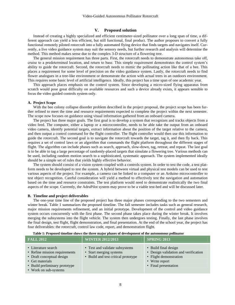
B. Timeline and project deliverables
The one-year time line of the proposed project has three major phases corresponding to the two semesters and
winter break. Table 1 summarizes the proposed timeline. The fall semester includes tasks such as general research,
major mission requirements refinement, and an initial prototype. Development of the control and video guidance
system occurs concurrently with the first phase. The second phase takes place during the winter break. It involves
merging the subsystems into the flight vehicle. The system then undergoes testing. Finally, the last phase involves
the final design, test flight, flight demonstration, and final presentation. At the end of the school year, the project has
four deliverables: the rotorcraft, control law code, report, and demonstration flight.
Table 1: Proposed timeline shows the three major phases of development of the autonomous pollinator
FALL 2012 WINTER 2012/2013 SPRING 2013
• Literature search
• Refine mission requirements
• Draft conceptual design
• Get materials
• Build preliminary prototype
• Work on sub-systems
• Test and validate subsystems
• Start merging systems
• Build and test critical prototype
• Build final design
• Design validation and verification
• Flight demonstration
• Write report
• Final presentation
Video-Guided Autonomous Pollinator Rotorcraft
9
VI. Image Recognition Programs and Hardware
A key program and some Arduino compatible cameras have been identified for the task of image recognition.
This is a major step forward as the project depends on the target recognition for successful completion.
A. OpenCV
OpenCV, which stands for “Open source Computer Vision”, is an open source library for C++ that has a variety
of image processing functions such as tracking and object recognition [26]. This program takes care of the bulk of
the work required in the Recognition portion of the project. Importantly, it is possible to integrate the image pro-
cessing algorithms with an Arduino microprocessor [27] for flight control.
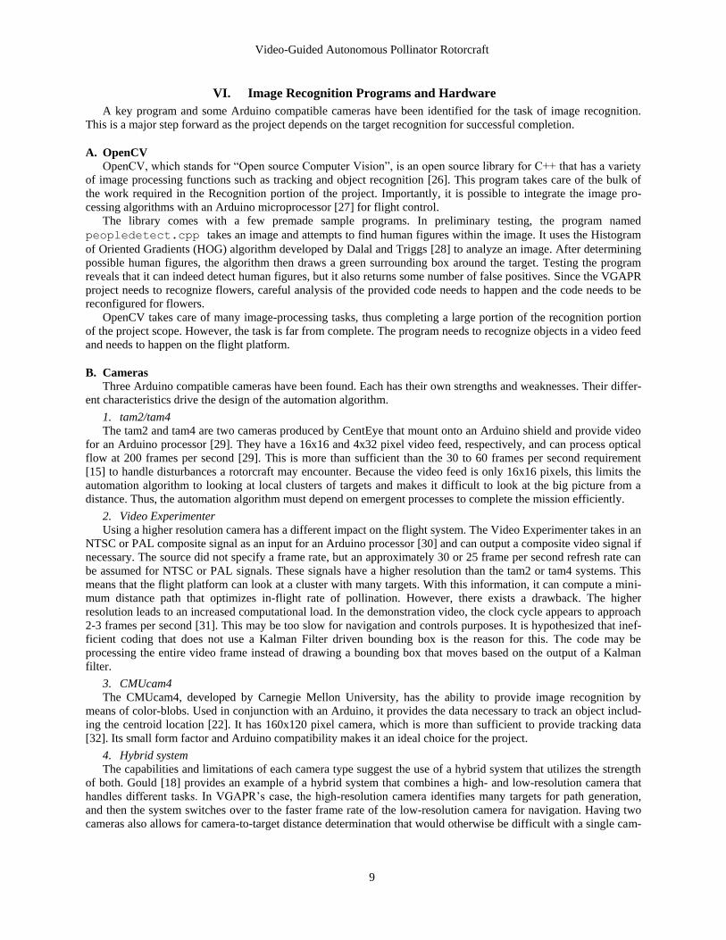
The library comes with a few premade sample programs. In preliminary testing, the program named
peopledetect.cpp takes an image and attempts to find human figures within the image. It uses the Histogram
of Oriented Gradients (HOG) algorithm developed by Dalal and Triggs [28] to analyze an image. After determining
possible human figures, the algorithm then draws a green surrounding box around the target. Testing the program
reveals that it can indeed detect human figures, but it also returns some number of false positives. Since the VGAPR
project needs to recognize flowers, careful analysis of the provided code needs to happen and the code needs to be
reconfigured for flowers.
OpenCV takes care of many image-processing tasks, thus completing a large portion of the recognition portion
of the project scope. However, the task is far from complete. The program needs to recognize objects in a video feed
and needs to happen on the flight platform.
B. Cameras
Three Arduino compatible cameras have been found. Each has their own strengths and weaknesses. Their differ-
ent characteristics drive the design of the automation algorithm.
1. tam2/tam4
The tam2 and tam4 are two cameras produced by CentEye that mount onto an Arduino shield and provide video
for an Arduino processor [29]. They have a 16x16 and 4x32 pixel video feed, respectively, and can process optical
flow at 200 frames per second [29]. This is more than sufficient than the 30 to 60 frames per second requirement
[15] to handle disturbances a rotorcraft may encounter. Because the video feed is only 16x16 pixels, this limits the
automation algorithm to looking at local clusters of targets and makes it difficult to look at the big picture from a
distance. Thus, the automation algorithm must depend on emergent processes to complete the mission efficiently.
2. Video Experimenter
Using a higher resolution camera has a different impact on the flight system. The Video Experimenter takes in an
NTSC or PAL composite signal as an input for an Arduino processor [30] and can output a composite video signal if
necessary. The source did not specify a frame rate, but an approximately 30 or 25 frame per second refresh rate can
be assumed for NTSC or PAL signals. These signals have a higher resolution than the tam2 or tam4 systems. This
means that the flight platform can look at a cluster with many targets. With this information, it can compute a mini-
mum distance path that optimizes in-flight rate of pollination. However, there exists a drawback. The higher
resolution leads to an increased computational load. In the demonstration video, the clock cycle appears to approach
2-3 frames per second [31]. This may be too slow for navigation and controls purposes. It is hypothesized that inef-
ficient coding that does not use a Kalman Filter driven bounding box is the reason for this. The code may be
processing the entire video frame instead of drawing a bounding box that moves based on the output of a Kalman
filter.
3. CMUcam4
The CMUcam4, developed by Carnegie Mellon University, has the ability to provide image recognition by
means of color-blobs. Used in conjunction with an Arduino, it provides the data necessary to track an object includ-
ing the centroid location [22]. It has 160x120 pixel camera, which is more than sufficient to provide tracking data
[32]. Its small form factor and Arduino compatibility makes it an ideal choice for the project.
4. Hybrid system
The capabilities and limitations of each camera type suggest the use of a hybrid system that utilizes the strength
of both. Gould [18] provides an example of a hybrid system that combines a high- and low-resolution camera that
handles different tasks. In VGAPR’s case, the high-resolution camera identifies many targets for path generation,
and then the system switches over to the faster frame rate of the low-resolution camera for navigation. Having two
cameras also allows for camera-to-target distance determination that would otherwise be difficult with a single cam-

Video-Guided Autonomous Pollinator Rotorcraft
10
era or require the use of a separate distance sensor. There exists a weight penalty for a two-camera set up. Ideally,
the final production design would be optimized for weight and would have an algorithm suitable for that set up.
5. Camera set-up
In order for the camera to know where the probe is, the initial design calls for the place of the probe within the
vision of the camera. This way, the camera can accurately detect if the probe has made contact with the target.
VII. Image Recognition Testing
While the OpenCV library can provide the image recognition and tracking algorithms that can fulfill the needs of
the project, continued research revealed a potentially serious compatibility problem of the library with the proposed
Arduino platform. The Arduino hardware may not have enough memory or processing power to handle the algo-
rithms required by the OpenCV libraries [33]. If the compatibility issue cannot be resolved, then the project cannot
move forward as image recognition is central to the project. However, the code does work with a webcam attached
to a computer. This means proof-of-concept testing can occur in the mean time with the OpenCV library.
A potential Arduino-compatible candidate called the CMUcam4 exists. The CMUcam4 has an embedded
160x120 pixel camera mounted on an Arduino Shield [34]. It also comes with an Arduino library to call built-in
image processing algorithms. The library has been shown to detect colors and control a robotic car with the Arduino
microprocessor [32]. If further verification shows compatibility for the project, a CMUcam4 will be used to provide
image recognition for the project.
A. Cascade Classifiers
While the exact device is being determined, further research into using an image recognition code to provide
simple control systems commands continued. An OpenCV code called objectDetection2.cpp written by
Huaman [35] detects faces and draws a bounding box around areas in the frame the code thinks a face exists. The
complete original code, with modifications shown in grey, can be found in Appendix C. The code first loads a .xml
file that contains a database of descriptors of the desired object for tracking. In Huaman’s code, the program calls on
a facial features library lbpcascade_frontalface.xml and an eye with, and without, eyeglasses library
haarcascade_eye_tree_eyeglasses.xml. The code then calls the function detectMultiScale() to
perform the image recognition using a video feed from a webcam and the aforementioned descriptors. The function
detectMultiScale() then outputs a class that contains the center and width and height of the areas of all de-
tected faces. The code uses that information to draw a circle around the detected faces that contain two eyes.
In order to execute the program, the user needs to open a command line console and call the compiled track-
er.exe file. The two .xml files need to be in the same folder as the tracker.exe file for the code to run
properly.
The initial trials show that the code could detect faces; however, it also has a problem with lag. The video lag is
estimated at around half a second between the frames. This amount of lag is significant and noticeable in use. It sug-
gests that something in the detection algorithm needs changing. Three potential changes include using a different
detection algorithm altogether, modifying the original code to make it quicker, or using a Kalman filter to create a
bounding box that reduces the computational area.
After noticing that larger eyes caused the algorithm to confirm detection of a face, the cause of the lag became
known. In order for the code to confirm facial detection, the code must also recognize two eyes inside the face. Re-
moving this portion of the code, below, increased the frame rate in the video feed.
eyes_cascade.detectMultiScale( faceROI, eyes,
1.1,
2,
0 |CV_HAAR_SCALE_IMAGE,
Size(5, 5));
The requirement for the detection of two eyes caused the lag noted previously. However, it does come with a draw-
back. The algorithm now detects many more false-positives. Thus, the requirement for having two eyes increased
the accuracy of the algorithm, but also slowed it down. With the two eyes requirement removed, the output is more
noisy, but the continuous face-detect rate increases and the lag decreases to a smaller amount.

Video-Guided Autonomous Pollinator Rotorcraft
11
B. Controls
The code needs modification to return important information for the navigation computer to use to command the
flight platform to a desired position. In this particular case, the image recognition should return commands that
cause the flight platform to center the desired object in the video frame. Thus, the code needs to output the offset
from the center of the detected object. Until the implementation of 3-D pose determination, the code should only
command the rotorcraft about the z -axis in early testing phases. This means the rotorcraft can take off and rotate
left and right only.
The control system needs a coordinate system defined first. Define the center of the frame as the origin and that
the frame has a u v axis system. Positive u and v means an object exists in the right half and upper half of the
frame, respectively. Then define a positive u command means a right yaw command and a positive v command
means an increase thrust command. Ideally, this command system causes the rotorcraft to take off and yaw only.
Realistically, the rotorcraft needs a few more sensors to ensure that it is not translating in any direction. This portion
of development shall come in the next few phases of development.
The code below uses the OpenCV command putText() to overlay the text onto the video feed.
char text2[255];
sprintf(text2,
"cmd(x, y) = (%d, %d)",
(faces[i].x + faces[i].width/2 - 640/2),
-(faces[i].y + faces[i].height/2 - 480/2));
putText(frame,
text2,
Point (100, 200),
FONT_HERSHEY_SIMPLEX,
1,
Scalar( 255, 255, 255 ),
2,
8,
false);
The navigation controller needs to take the command yaw and thrust, in pixels and convert it into a useful number
for controlling the rotorcraft. Currently, the code displays the offset for all detected objects. Further development
would require a filter that reduces the number of false-positives.
C. Ranging
The code also returns the dimensions of the detected object that can provide a subject to camera distance estima-
tion. This information allows the navigation computer to avoid collision and know when to stop moving forward
after contact has been made with the target.
The OpenCV documentation provides a complete equation for the pinhole camera model [36].
11 12 13 1
21 22 23 2
31 32 33 3
' | '
0
0
0 0 111
x x
y y
sm A R t M
Xu f c r r r t
Ys v f c r r r t
Zr r r t
(1)
This equation shows the complete transformation for a point in 3-D space onto a 2-D image space. It takes in a point
, ,X Y Z in 3-D space in vector 'M , convolves it with a translation/rotation matrix |R t and an intrinsic camera
properties matrix A , and outputs a point on a 2-D frame in the vector 'm .
The code experiments with a simplified pinhole camera model. It assumes that the camera has a viewing angle
that encompasses the imaging device width w , in pixels. An object of a known size h and distance d exists in the 3-
D space and has an image height i, in pixels, on the imaging device. The function detectMultiScale() outputs
Video-Guided Autonomous Pollinator Rotorcraft
12
the value i. The angular coverage of the object , common to the 3-D and 2-D space, equals the inverse tangent of
the image width divided by the focal length f,
tani
f
(2)
The focal length can be calculated from the camera viewing angle and the video frame width,
tan
wf
(3)
Since the angular coverage of the image and the object must be the same,
1 1tan tani h
f d
(4)
Thus,
i h
f d
(5)
Substituting for focal length f,
/ tan
i h
w d
(6)
Solving for the distance d,
tan
h wd
i
(7)
This model requires the key assumption that all objects have a uniform height. An experiment consisting of the
measurement of five college-aged male faces yielded an average facial height of 8 inches from the chin to the hair-
line and a single female facial height of 7 inches. The model uses the modal average value of 8 inches for the
computation of the distance.
The next portion of the experiment tests the accuracy of the model in practice. An iHome IH-W320BS webcam
provided a 640x480 pixel video stream via a USB cable. To determine the camera’s angle of view, two straight edg-
es and the camera were placed on a table. The straight edges converged at the camera’s focal point and extended out
such that they created a straight line on the left and right edge of the image. The angle was measured by taking the
inverse tangent of a known length on the straight edge and the right angle distance to the other edge. After taking
measurements, the camera has an estimated horizontal angle of view of 40 degrees.
After determining the camera view angle, run the tracker.exe program. Place a face in front of the camera
and record the pixel width of the detected face and the distance between the face and the camera’s focal point. Last-
ly, record the data in Excel.
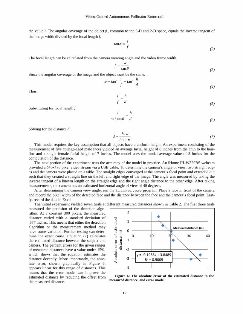
The initial experiment yielded seven trials at different measured distances shown in Table 2. The first three trials
measured the precision of the detection algo-
rithm. At a constant 300 pixels, the measured
distance varied with a standard deviation of
.577 inches. This means that either the detection
algorithm or the measurement method may
have some variation. Further testing can deter-
mine the exact cause. Equation (7) calculates
the estimated distance between the subject and
camera. The percent errors for the given ranges
of measured distances have a value under 15%,
which shows that the equation estimates the
distance decently. More importantly, the abso-
lute error, shown graphically in Figure 6,
appears linear for this range of distances. This
means that the error model can improve the
estimated distance by reducing the offset from
the measured distance.
Figure 6: The absolute error of the estimated distance to the
measured distance, and error model.
y = -0.1986x + 3.8489 R² = 0.9009
-4
-3
-2
-1
0
1
2
0 10 20 30 40
Ab
solu
te e
rro
r o
f es
tim
ated
d
ista
nce
(in
)
Measured distance (in)
Video-Guided Autonomous Pollinator Rotorcraft
13
The results show that there exists some amount of error in the estimated distance. However, the error varies line-
arly with distance and a reduction model exists to reduce the error. The assumption that the subject size remains the
same from subject to subject is crucial to this model.
Table 2: Measured camera-to-subject distances and reported image widths
Trial 1 2 3 4 5 6 7
Measured distance (in) 20.5 21.5 20.5 16.0 31.0 36.0 13.7
Pixels 300 300 300 371 220 184 404
Estimated distance (in) 20.5 20.5 20.5 16.6 27.9 33.4 15.2
Percent difference 0.1% 5.0% 0.1% 3.4% 11.0% 7.8% 9.9%
Absolute difference (in) 0.0 -1.0 0.0 0.6 -3.1 -2.6 1.5
D. CMUcam4
At the core of the flight platform is the CMUcam4. Verification of its image recognition abilities is an important
step in the progress of the project. To power it up, it is connected as a shield to the Arduino for power. A laptop pro-
vides the electricity to the Arduino via a USB cable. This also boots up the CMUcam4. By pressing and holding the
reset and the user button, the CMUcam4 enters demo mode.
In this mode, the board tracks the object placed in front of the camera. The board then outputs the video stream
through an RCA video out port. Hooking this port with a television allows the user to see what the image processor
currently tracks. The image is a black background with blue color blobs that represent the color blobs the image
recognition program detects as a target. It also draws a bounding box around the object and a dot at the centroid of
the blob.
The servo signals also needed verification as these signals eventually are inputted into the microcontroller. To
verify these signals, a servo with a linkage arm is connected (along with a separate battery for power) to the pan and
tilt ports on the CMUcam4. In demo mode, the CMUcam4 sends servo signals to the pan and tilt outputs that can
move the servo arm. By moving the tracked object relative to the camera, the servo arm moves accordingly. Howev-
er, testing revealed that the servo arm moves slowly when a step function occurs in the movement of the tracked
object. The cause of the rotational velocity saturation has not been determined yet. Current hypotheses point to low
battery power, a faulty servo, or the signal actually has significant lag. Further testing identifies the source of the lag.
Parameter identification, performed later, models the lag in the control system design [37].
Careful review of the function library documentation reveals the option to vary the proportional and derivative
gain. By increasing these values, the response of the servo increases. The servo responds more quickly to step func-
tions. However, servo testing shows that the servo signal continues to diverge after a step function input. This
suggests an integral behavior in the control system, and that the proportional/derivative gains may in fact be misla-
beled integral/proportional gains. Analysis with CIFER on page 34 below concludes that the gains indeed are
mislabeled.
CHANGE IN
TARGET POSITION
CAMERA
OUTPUT: VIDEO SIGNAL
IMAGE PROCESSOR
OUTPUT: TARGET DATA
NAVIGATION PROCESSOR
OUTPUT: COMMANDS
ROTORCRAFT
DYNAMICS
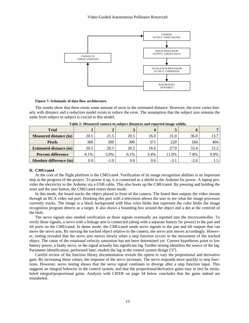
Figure 7: Schematic of data flow architecture.

Video-Guided Autonomous Pollinator Rotorcraft
14
The CMUcam4 can also provide ranging data. According to the documentation [22], the device can return a t-
type data on the tracked pixels coverage percentage. This value can provide the information required to perform
ranging. Using equations, the distance of a target with a known size can be determined.
In conclusion, the device should fulfill the needs of the system to carry out the mission. It can determine the ob-
ject offset from the camera, send control signals, and potentially provide ranging information to the microprocessor
for the development of the control algorithm.
VIII. Navigation and Automation: Initial High-Level Algorithms
A. Mission/Flight Profile
The VGAPR’s mission profile has three legs. The departure leg occurs at the beginning of the flight mission.
The rotorcraft takes off from the home base and flies towards the orchard. Once it gets there, it starts the pollination
algorithm. This leg lasts until it tags all targets, until battery levels run low, or if there is a system error. For the pur-
poses of the project, the orchard is replaced by an indoors tree simulator structure. This structure would have
randomly placed targets that the rotorcraft needs to tag.
B. Navigation model
At a high level, the flight platform has two microprocessors. Like a computer, the navigation processor handles
‘thinking’ problems (analogous to a CPU), while the image processor handles graphics problems (analogous to a
GPU). This may be necessary to address the limited processing power of an Arduino board. Figure 7 shows a sche-
matic of the high-level architecture.
It begins with the video feed from camera into the image processor. The image processor then identifies the tar-
gets and critical data required by the navigation processor and sends the information there. The navigation processor
then determines a path to follow and sends commands to the motors (for a quadrotor) or the motors and vanes (for a
ducted fan). The navigation processor also handles stability for the flight platform as well. The motion of the ro-
torcraft then changes the position of the targets, which the camera picks up and the loop starts over again.
Another aspect of the navigation model is the different phases of the pollination processes. The flight level polli-
nation algorithm is inspired by Saripelli’s landing algo-
rithm [19] [9]. The key phase is the approach/contact
/departure maneuver required to tag a flower. Figure 8
graphically shows various stages of the algorithm. This
maneuver is basically an in-flight touch-and-go version
of Saripelli’s landing algorithm. After the touch and go,
the system needs to find the next target. How it does this
is determined by the automation routine.
C. Automation model
As mentioned in the section discussing the two types
of camera options, the choice of camera influences the
structure of the automation model. A different model fits
each camera choice. For a high-resolution camera, the
processor can attempt to solve for a minimum distance
path that efficiently pollinates all targets, thus solving a
traveling salesman problem. This is computationally
expensive as it is NP-hard and no known general solu-
tion exists [38]. Figure 9 shows an example of a reduced
total-distance solution to a problem. However, given
that each sampled section is small enough, it may be
worthwhile to solve for the smallest total-distance to
cover all points. However, if only a low-resolution cam-
era is used, then simple processes would work better. A
basic algorithm is to sweep the entire test area, either
linearly or in a spiral. This brute force method guaran-
tees coverage of all surveyable areas. Another viable
method works by simply visiting the nearest unvisited
neighbor. The path would appear chaotic, but this
SEE NEXT
TARGET?
MOVE BACK
AND
SEARCH
TRACK AND MOVE
CLOSER
HAVE
CONTACT?
MOVE BACK
NO
YES No
YES
Figure 8: Proposed Touch-and-Go algorithm.

Video-Guided Autonomous Pollinator Rotorcraft
15
process maximizes tagging rates. In order for this
method to work, the flight computer needs to have a
Simultaneous Localization and Mapping (SLAM)
algorithm. However, this method does not guarantee
coverage of all surveyable areas unless the flight
computer remembers to visit unvisited areas. A
computer simulation will test these models to see
which ones perform well given the constraints of the
video system.
D. Traveling Salesman Problem
The initial attempt at solving the traveling sales-
man problem using MATLAB had some success. A
traveling salesman good algorithm attempts to find a
sufficiently good, short path that visits a set of given
points. The Maple code published by Betten [39] creates a random tour, swaps two legs, and compares the cost of
the old and new path to find a better path.
The developed MATLAB algorithm (still currently under development and can be found in Appendix B) has a
slightly different structure. It looks for the longest path between any two points and swaps it for the nearest neigh-
bor. The algorithm works for one or two iterations at most, then stopped. The path did get shorter, however. Further
examination can reveal the problem with the code. However, development of this code stopped until more basic
control problems such as identification and ranging have been solved.
IX. Systems Testing Plan
Towards the end of the design process, the integrated system needs validation. A flight platform will undergo a
series of tests to check each system. The tests increase in complexity and tests the systems incrementally. The fol-
lowing outlines a proposed test procedure in the event that all systems are ready in time within the project timeline.
A. Flight platform
The testing of the flight algorithm will be done on the most accessible platform. Current options include the
quadrotor and the ducted fan. The quadrotor uses four motors to control plant dynamics. This makes maneuvering a
simple task for the navigation processor. The camera would be placed on the same side as the pollinator probe to
optimize visibility and other systems hardware would be placed accordingly to provide balance. Alternatively, a
vertical ducted fan can also meet the mission requirements of vertical flight. It has the benefit of being small and
light as it only has one motor for propulsion. Vanes beneath the ducted fan control the flight platform. The camera
would also be placed on the same side as the probe to provide visibility and the systems hardware would be placed
accordingly to provide balance. Production models should use the smallest flight platform possible that incorporates
an optimal form of all the systems sued in the platform. Possibilities include a flapping-wing design used by Har-
vard’s RoboBee project.
B. 0-D model
In the 0-D model, the camera and test subject stay stationary. The image processor then needs to recognize the
test target and generate key parameters including position and distance. If the system has a Kalman filter, the bound-
ing box needs to move and be resized appropriately.
C. 1-D model
This model tests the touch-and-go algorithm. It requires a working range determination system. Initial research
shows that ranging is possible for a single camera if other parameters are known [40]. If a single camera cannot ef-
fectively determine range, alternative methods can be used. For example, two cameras can use parallax to calculate
range, or an ultrasonic sensor can do the same. The 1-D test would test the effectiveness of these options. Addition-
ally, take-off and landing can be tested here, too.
D. 2-D model
After verification of the basic controls, testing can proceed with a 2-D target model. The flight platform now
needs to translate forward, backward, left, right, and yaw. The system should now be able to move from target to
Figure 9: An example of a solution on the right of a random
set of points [38]. The solution to this problem yields a shorter
path travelled than a linear brute-force method. However, it is
computationally expensive.

Video-Guided Autonomous Pollinator Rotorcraft
16
target, but not tag them. This model tests the navigation and automation algorithms. The test patterns will be ar-
ranged in a 2-D plane representative of a segment of a tree.
E. 3-D model
This model fully tests all systems completely. Initial 3-D testing can be done on the 2-D model mentioned above,
but now incorporates tagging. Upon successful demonstration of this, a spherical tree model shall test the ro-
torcraft’s ability to move around a curve. Finally, the flight platform needs to navigate from tree to tree.
X. Arduino Development
A. Servo control with Arduino
Servos take in a commanded signal and use it to drive a servomechanism. The servo signals tend use pulse
width modulation (PWM) for articulation. The servos read pulses that last between 1000 and 2000 microseconds
sent at 20 millisecond intervals [41]. Servos respond to the varying the duration of the pulse widths. For example, a
pulse width of 1000 microseconds can mean full left aileron on an airplane or full left roll on a quadrotor and 2000
microseconds can mean full right aileron on an airplane or full right roll on a quadrotor. In order for an Arduino to
read these signals and perform other functions simultaneously requires the use of interrupts.
Interrupts allow the Arduino to perform other tasks while waiting for a change of state from the servo signal. At
a computer processor’s time scale, the servo signal does not change. Using a function such as pulseIn() measures the length of the pulse width, the measurement of interest. However, this prevents the Arduino from per-
forming any other functions during the duration of the measurement. This results in slow performance as the
microcontroller can perform 320,000 operations during the 20 milliseconds between each pulse.
In order to read the many servo signals required, this project uses the pinChangeInt.h library. The Arduino
UNO comes with two interrupts on digital pins 2 and 3 by default [42]. The pinChangeInt.h library expands
this capability to all 20 pins.
B. Input/output
The Arduino needs to be able to read
inputs from a few sources and send out-
puts to subsystems that require data.
The first input comes from the re-
ceiver. The receiver connects wirelessly
to a pilot controlled transmitter. The pilot
commands roll, pitch, yaw, throttle, and auxiliary signals. The auxiliary signal allows the pilot to control the
quadrotor and switch the quadrotor into testing mode to verify autonomous routines.
The second input comes from the CMUcam4’s pan and tilt servo outputs. The tilt signal can be used to increase
or decrease the altitude of the quadrotor as it correlates to a difference in altitude between a detected object and the
camera. The pan servo can be used to control yaw or roll depending on the mode required for testing.
The third signal communicates bidirectionally between the Arduino and the CMUcam4. This uses digital pins 0
and 1 on the Arduino. This channel allows the Arduino to send commands to the CMUcam4 board as well as receive
information such as target size from the CMUcam4.
The fourth channel uses the analog pins 4 and 5 to communicate with the MPU-6050 IMU. This unit provides
acceleration and roll rates to the Arduino. The acceleration data can be used to level the quadrotor. In steady level
hover, the gravity vector points entirely in the negative z-axis only. This can be achieved by zeroing any x or y com-
ponents of acceleration. Acceleration can provide the necessary initial attitude conditions for the rate gyro to
integrate attitude.
The fifth set of channels output servo signals to the control board. The Arduino combines all of the inputs and
computes an output for the control board. The signals include only roll, pitch, yaw, and throttle servo signals. In
essence, the Arduino should replace a human pilot when properly configured.
Figure 10: A visual representation of a servo signal [41].

Video-Guided Autonomous Pollinator Rotorcraft
17
C. Libraries and Functions
The following section outlines key functions provided by their respective authors that are used in this project.
Library Name Function name Description Notes
CMUcam4 automaticPan()/
automaticTilt() Enables the pan and tilt
servo outs to send sig-
nals.
Servo signal responds to the error of the
centroid from the center of the frame.
Can be turned on or off individually. autoPanParameters()/
autoTiltParameters() Allows the adjustment
of gain parameters for
servo signal outs. Can
be adjusted to values
between 0 and 1000.
Preliminary testing shows that gains are
mislabeled and are actually integral and
proportional gains. For example, when
proportionalGain is set to 1000 and
derivativeGain to 0, the servo signal
gets integrated and becomes saturated
over time with a step error. When
derivativeGain is set to 1000, servo
responds proportionally to error, i.e. the
servo signal tracks the error. noiseFilter() Ignores blobs smaller
than the input value for
the purposes of tracking
For example, a noise filter of strength 2
filters out “the leading two pixels in any
group of pixels in a row” Whether this
removes blobs or consecutive blocks for
values larger than 2 is unknown. trackColor() Tells CMUcam4 what
colors to track
Inputs in RGB values by default. YUV
color space available, but not used. Best
option is to use bright colors such as
plane white light sources. Testing uses
off whites to pure whites from (252, 252,
252) to (255, 255, 255). Multiple targets
can be set if different colors are used.
Bright primary and secondary colors are
recommended for tracking getTypeTDataPacket() Gets tracking data from
CMUcam4. Returns
pixels, confi-
dence, mx, my
Pixels is the screen percent coverage
of a detected color. The value of pixels
can be used to determine the range of the
target if the size is known a priori.
Confidence correlates to the ratio be-
tween the detected area and the area of
the bounding box that the detected colors
exist in. High confidence values mean
that the target colors cover a large portion
of the bounding box.
mx and my correspond to the position of
the centroid of the detected blob with the
origin in one of the image corners. servo writeMicroseconds() Writes a servo signal to
a servo pin
pinChangeInt attachInterrupt() Allows a pin to handle
interrupts
This library expands the interrupt capa-
bilities of an Arduino UNO to all pins.
D. SparkFun MPU-6050 Inertial Measurement Unit
The SparkFun MPU-6050 IMU measures 3 axis acceleration and 3 axis rotation rates. The breakout board
measures 1x0.6x0.1 inches. The board connects to the Arduino with four wires: a 3.3V line, a ground, an SDA line,
Video-Guided Autonomous Pollinator Rotorcraft
18
and an SCL line. The accelerometer has selectable ranges from ±2g, ±4g, ±8g, and ±16g. The gyro has selectable
ranges from ±250, ±500, ±1000, and ±2000 degrees per second [43].
In hover flight with no disturbances, the gravity acceleration vector points entirely in the negative z-axis with ze-
ro x and y components. The control law can use this information to drive the x and y acceleration components to
zero. This results in pitch and roll commands that yield corrective action to drive the flight platform into a level po-
sition. Drift may occur due to errors in mounting the accelerometer on the flight platform. Weights can be attached
to the quadrotor to negate drift.
More importantly, the accelerometer data can provide information on attitude. The arctangent of the ratio be-
tween x and y accelerations to the z acceleration provides the pitch and roll angles, respectively. Equations (8) and
(9) shows the relationship between accelerations and the pitch angle and the roll angle .
arctan x
z
a
a
(8)
arctany
z
a
a
(9)
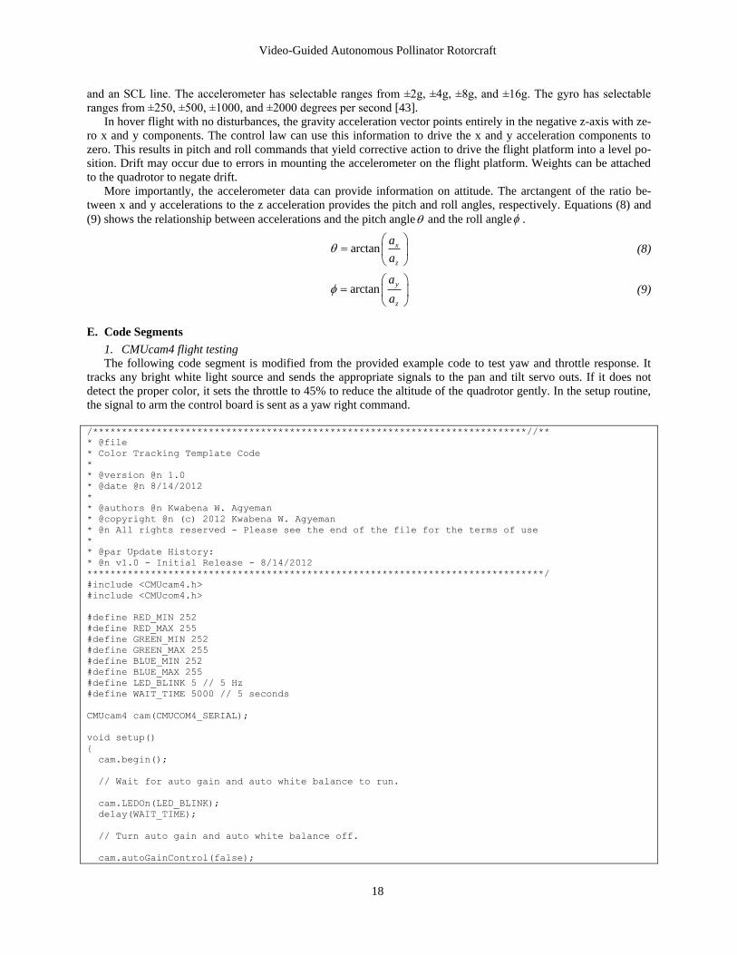
E. Code Segments
1. CMUcam4 flight testing
The following code segment is modified from the provided example code to test yaw and throttle response. It
tracks any bright white light source and sends the appropriate signals to the pan and tilt servo outs. If it does not
detect the proper color, it sets the throttle to 45% to reduce the altitude of the quadrotor gently. In the setup routine,
the signal to arm the control board is sent as a yaw right command.
/***************************************************************************//**
* @file
* Color Tracking Template Code
*
* @version @n 1.0
* @date @n 8/14/2012
*
* @authors @n Kwabena W. Agyeman
* @copyright @n (c) 2012 Kwabena W. Agyeman
* @n All rights reserved - Please see the end of the file for the terms of use
*
* @par Update History:
* @n v1.0 - Initial Release - 8/14/2012
*******************************************************************************/
#include <CMUcam4.h>
#include <CMUcom4.h>
#define RED_MIN 252
#define RED_MAX 255
#define GREEN_MIN 252
#define GREEN_MAX 255
#define BLUE_MIN 252
#define BLUE_MAX 255
#define LED_BLINK 5 // 5 Hz
#define WAIT_TIME 5000 // 5 seconds
CMUcam4 cam(CMUCOM4_SERIAL);
void setup()
{
cam.begin();
// Wait for auto gain and auto white balance to run.
cam.LEDOn(LED_BLINK);
delay(WAIT_TIME);
// Turn auto gain and auto white balance off.
cam.autoGainControl(false);

Video-Guided Autonomous Pollinator Rotorcraft
19
cam.autoWhiteBalance(false);
cam.automaticPan(true, false); // Turn panning on.
cam.automaticTilt(true, false); // Turn tilting on.
cam.autoPanParameters(50, 1000); // Yaw gains
cam.autoTiltParameters(25, 100); //Throttle Gains
cam.setServoPosition(1,1,1000); // Kill throttle
cam.setServoPosition(0,1,2000); // Arm control board: yaw right
delay(WAIT_TIME - 3000);
//cam.LEDOn(CMUCAM4_LED_ON);
cam.LEDOff();
cam.noiseFilter(10);
}
void loop()
{
CMUcam4_tracking_data_t data;
cam.trackColor(RED_MIN, RED_MAX, GREEN_MIN, GREEN_MAX, BLUE_MIN, BLUE_MAX);
for(;;)
{
cam.getTypeTDataPacket(&data); // Get a tracking packet.
if(cam.getButtonPressed() == true)
{
cam.setServoPosition(1,1,1000);
delay(100);
cam.setServoPosition(0,1,1000);
delay(WAIT_TIME);
}
else if (data.pixels > 01 && data.confidence > 60) // If detection, track object
{
cam.LEDOn(CMUCAM4_LED_ON);
cam.automaticPan(true, false); // Turn panning on.
cam.automaticTilt(true, false); // Turn Tilt on
break;
}
else // If no detection, stop turning and throttle off
{
cam.LEDOff();
cam.automaticPan(false, false); // Turn panning on.
cam.automaticTilt(false, false);
cam.setServoPosition(0,1,1500);
cam.setServoPosition(1,1,1450); // Throttle to 45%
break;
}
}
}
/***************************************************************************//**
* @file
* @par MIT License - TERMS OF USE:
* @n Permission is hereby granted, free of charge, to any person obtaining a
* copy of this software and associated documentation files (the "Software"), to
* deal in the Software without restriction, including without limitation the
* rights to use, copy, modify, merge, publish, distribute, sublicense, and/or
* sell copies of the Software, and to permit persons to whom the Software is
* furnished to do so, subject to the following conditions:
* @n
* @n The above copyright notice and this permission notice shall be included in
* all copies or substantial portions of the Software.
* @n
* @n THE SOFTWARE IS PROVIDED "AS IS", WITHOUT WARRANTY OF ANY KIND, EXPRESS OR
* IMPLIED, INCLUDING BUT NOT LIMITED TO THE WARRANTIES OF MERCHANTABILITY,
* FITNESS FOR A PARTICULAR PURPOSE AND NONINFRINGEMENT. IN NO EVENT SHALL THE
* AUTHORS OR COPYRIGHT HOLDERS BE LIABLE FOR ANY CLAIM, DAMAGES OR OTHER
* LIABILITY, WHETHER IN AN ACTION OF CONTRACT, TORT OR OTHERWISE, ARISING FROM,
* OUT OF OR IN CONNECTION WITH THE SOFTWARE OR THE USE OR OTHER DEALINGS IN THE
* SOFTWARE.
*******************************************************************************/

Video-Guided Autonomous Pollinator Rotorcraft
20
2. Reading multiple servo signals
In order to read the numerous signals required by the project, the code provided by RCArduino has been modi-
fied to add more channels to the interrupt routine.
// MultiChannels
//
// rcarduino.blogspot.com
//
// A simple approach for reading three RC Channels using pin change interrupts
//
// See related posts -
// http://rcarduino.blogspot.co.uk/2012/01/how-to-read-rc-receiver-with.html
// http://rcarduino.blogspot.co.uk/2012/03/need-more-interrupts-to-read-more.html
// http://rcarduino.blogspot.co.uk/2012/01/can-i-control-more-than-x-servos-with.html
//
// rcarduino.blogspot.com
//
// include the pinchangeint library - see the links in the related topics section above for de-
tails
#include <PinChangeInt.h>
#include <Servo.h>
// Assign your channel in pins
#define THROTTLE_IN_PIN 8
#define STEERING_IN_PIN 9
#define AUX_IN_PIN 10
#define AUX2_IN_PIN 11
// Assign your channel out pins
#define AUX2_OUT_PIN 4
#define THROTTLE_OUT_PIN 5
#define STEERING_OUT_PIN 6
#define AUX_OUT_PIN 7
// Servo objects generate the signals expected by Electronic Speed Controllers and Servos
// We will use the objects to output the signals we read in
// this example code provides a straight pass through of the signal with no custom processing
Servo servoThrottle;
Servo servoSteering;
Servo servoAux;
Servo servoAux2;
// These bit flags are set in bUpdateFlagsShared to indicate which
// channels have new signals
#define THROTTLE_FLAG 1
#define STEERING_FLAG 2
#define AUX_FLAG 4
#define AUX2_FLAG 8
// holds the update flags defined above
volatile uint8_t bUpdateFlagsShared;
// shared variables are updated by the ISR and read by loop.
// In loop we immediatley take local copies so that the ISR can keep ownership of the
// shared ones. To access these in loop
// we first turn interrupts off with noInterrupts
// we take a copy to use in loop and the turn interrupts back on
// as quickly as possible, this ensures that we are always able to receive new signals
volatile uint16_t unThrottleInShared;
volatile uint16_t unSteeringInShared;
volatile uint16_t unAuxInShared;
volatile uint16_t unAux2InShared;
// These are used to record the rising edge of a pulse in the calcInput functions
// They do not need to be volatile as they are only used in the ISR. If we wanted
// to refer to these in loop and the ISR then they would need to be declared volatile
uint32_t ulThrottleStart;
uint32_t ulSteeringStart;

Video-Guided Autonomous Pollinator Rotorcraft
21
uint32_t ulAuxStart;
uint32_t ulAux2Start;
void setup()
{
Serial.begin(9600);
Serial.println("multiChannels");
// attach servo objects, these will generate the correct
// pulses for driving Electronic speed controllers, servos or other devices
// designed to interface directly with RC Receivers
servoThrottle.attach(THROTTLE_OUT_PIN);
servoSteering.attach(STEERING_OUT_PIN);
servoAux.attach(AUX_OUT_PIN);
servoAux2.attach(AUX2_OUT_PIN);
// using the PinChangeInt library, attach the interrupts
// used to read the channels
PCintPort::attachInterrupt(THROTTLE_IN_PIN, calcThrottle,CHANGE);
PCintPort::attachInterrupt(STEERING_IN_PIN, calcSteering,CHANGE);
PCintPort::attachInterrupt(AUX_IN_PIN, calcAux,CHANGE);
PCintPort::attachInterrupt(AUX2_IN_PIN, calcAux2,CHANGE);
}
void loop()
{
// create local variables to hold a local copies of the channel inputs
// these are declared static so that thier values will be retained
// between calls to loop.
static uint16_t unThrottleIn;
static uint16_t unSteeringIn;
static uint16_t unAuxIn;
static uint16_t unAux2In;
// local copy of update flags
static uint8_t bUpdateFlags;
// check shared update flags to see if any channels have a new signal
if(bUpdateFlagsShared)
{
noInterrupts(); // turn interrupts off quickly while we take local copies of the shared vari-
ables
// take a local copy of which channels were updated in case we need to use this in the rest
of loop
bUpdateFlags = bUpdateFlagsShared;
// in the current code, the shared values are always populated
// so we could copy them without testing the flags
// however in the future this could change, so lets
// only copy when the flags tell us we can.
if(bUpdateFlags & THROTTLE_FLAG)
{
unThrottleIn = unThrottleInShared;
}
if(bUpdateFlags & STEERING_FLAG)
{
unSteeringIn = unSteeringInShared;
}
if(bUpdateFlags & AUX_FLAG)
{
unAuxIn = unAuxInShared;
}
if(bUpdateFlags & AUX2_FLAG)
{
unAux2In = unAux2InShared;
}

Video-Guided Autonomous Pollinator Rotorcraft
22
// clear shared copy of updated flags as we have already taken the updates
// we still have a local copy if we need to use it in bUpdateFlags
bUpdateFlagsShared = 0;
interrupts(); // we have local copies of the inputs, so now we can turn interrupts back on
// as soon as interrupts are back on, we can no longer use the shared copies, the interrupt
// service routines own these and could update them at any time. During the update, the
// shared copies may contain junk. Luckily we have our local copies to work with :-)
}
// do any processing from here onwards
// only use the local values unAuxIn, unThrottleIn and unSteeringIn, the shared
// variables unAuxInShared, unThrottleInShared, unSteeringInShared are always owned by
// the interrupt routines and should not be used in loop
// the following code provides simple pass through
// this is a good initial test, the Arduino will pass through
// receiver input as if the Arduino is not there.
// This should be used to confirm the circuit and power
// before attempting any custom processing in a project.
// we are checking to see if the channel value has changed, this is indicated
// by the flags. For the simple pass through we don't really need this check,
// but for a more complex project where a new signal requires significant processing
// this allows us to only calculate new values when we have new inputs, rather than
// on every cycle.
if(bUpdateFlags & THROTTLE_FLAG)
{
if(servoThrottle.readMicroseconds() != unThrottleIn)
{
servoThrottle.writeMicroseconds(unThrottleIn);
}
}
if(bUpdateFlags & STEERING_FLAG)
{
if(servoSteering.readMicroseconds() != unSteeringIn)
{
servoSteering.writeMicroseconds(unSteeringIn);
}
}
if(bUpdateFlags & AUX_FLAG)
{
if(servoAux.readMicroseconds() != unAuxIn)
{
servoAux.writeMicroseconds(unAuxIn);
}
}
if(bUpdateFlags & AUX2_FLAG)
{
if(servoAux2.readMicroseconds() != unAux2In)
{
servoAux2.writeMicroseconds(unAux2In);
}
}
Serial.println(unAux2In);
bUpdateFlags = 0;
}
// simple interrupt service routine
void calcThrottle()
{
// if the pin is high, its a rising edge of the signal pulse, so lets record its value
if(digitalRead(THROTTLE_IN_PIN) == HIGH)
{
ulThrottleStart = micros();
}

Video-Guided Autonomous Pollinator Rotorcraft
23
else
{
// else it must be a falling edge, so lets get the time and subtract the time of the rising
edge
// this gives use the time between the rising and falling edges i.e. the pulse duration.
unThrottleInShared = (uint16_t)(micros() - ulThrottleStart);
// use set the throttle flag to indicate that a new throttle signal has been received
bUpdateFlagsShared |= THROTTLE_FLAG;
}
}
void calcSteering()
{
if(digitalRead(STEERING_IN_PIN) == HIGH)
{
ulSteeringStart = micros();
}
else
{
unSteeringInShared = (uint16_t)(micros() - ulSteeringStart);
bUpdateFlagsShared |= STEERING_FLAG;
}
}
void calcAux()
{
if(digitalRead(AUX_IN_PIN) == HIGH)
{
ulAuxStart = micros();
}
else
{
unAuxInShared = (uint16_t)(micros() - ulAuxStart);
bUpdateFlagsShared |= AUX_FLAG;
}
}
void calcAux2()
{
if(digitalRead(AUX2_IN_PIN) == HIGH)
{
ulAux2Start = micros();
}
else
{
unAux2InShared = (uint16_t)(micros() - ulAux2Start);
bUpdateFlagsShared |= AUX2_FLAG;
}
}
3. MPU-6050 IMU
To test the IMU, the following segment of code is used. It has been modified from the original to output a servo
signal based on the gryo output. The code can also be modified to incorporate acceleration data as well.
#include <Servo.h>
// I2C device class (I2Cdev) demonstration Arduino sketch for MPU6050 class
// 10/7/2011 by Jeff Rowberg <[email protected]>
// Updates should (hopefully) always be available at https://github.com/jrowberg/i2cdevlib
//
// Changelog:
// 2011-10-07 - initial release
/* ============================================
I2Cdev device library code is placed under the MIT license
Copyright (c) 2011 Jeff Rowberg
Permission is hereby granted, free of charge, to any person obtaining a copy
of this software and associated documentation files (the "Software"), to deal

Video-Guided Autonomous Pollinator Rotorcraft
24
in the Software without restriction, including without limitation the rights
to use, copy, modify, merge, publish, distribute, sublicense, and/or sell
copies of the Software, and to permit persons to whom the Software is
furnished to do so, subject to the following conditions:
The above copyright notice and this permission notice shall be included in
all copies or substantial portions of the Software.
THE SOFTWARE IS PROVIDED "AS IS", WITHOUT WARRANTY OF ANY KIND, EXPRESS OR
IMPLIED, INCLUDING BUT NOT LIMITED TO THE WARRANTIES OF MERCHANTABILITY,
FITNESS FOR A PARTICULAR PURPOSE AND NONINFRINGEMENT. IN NO EVENT SHALL THE
AUTHORS OR COPYRIGHT HOLDERS BE LIABLE FOR ANY CLAIM, DAMAGES OR OTHER
LIABILITY, WHETHER IN AN ACTION OF CONTRACT, TORT OR OTHERWISE, ARISING FROM,
OUT OF OR IN CONNECTION WITH THE SOFTWARE OR THE USE OR OTHER DEALINGS IN
THE SOFTWARE.
===============================================
*/
// Arduino Wire library is required if I2Cdev I2CDEV_ARDUINO_WIRE implementation
// is used in I2Cdev.h
#include "Wire.h"
// I2Cdev and MPU6050 must be installed as libraries, or else the .cpp/.h files
// for both classes must be in the include path of your project
#include "I2Cdev.h"
#include "MPU6050.h"
// class default I2C address is 0x68
// specific I2C addresses may be passed as a parameter here
// AD0 low = 0x68 (default for InvenSense evaluation board)
// AD0 high = 0x69
MPU6050 accelgyro;
int16_t ax, ay, az;
int16_t gx, gy, gz;
int gxdot;
int gx0;
Servo myServo;
#define LED_PIN 13
bool blinkState = false;
int ms;
void setup() {
// join I2C bus (I2Cdev library doesn't do this automatically)
Wire.begin();
// initialize serial communication
// (38400 chosen because it works as well at 8MHz as it does at 16MHz, but
// it's really up to you depending on your project)
Serial.begin(38400);
// initialize device
Serial.println("Initializing I2C devices...");
accelgyro.initialize();
accelgyro.setFullScaleGyroRange(MPU6050_GYRO_FS_250);
// verify connection
Serial.println("Testing device connections...");
Serial.println(accelgyro.testConnection() ? "MPU6050 connection successful" : "MPU6050 con-
nection failed");
// configure Arduino LED for
pinMode(LED_PIN, OUTPUT);
myServo.attach(9);
}
void loop() {

Video-Guided Autonomous Pollinator Rotorcraft
25
// read raw accel/gyro measurements from device
accelgyro.getMotion6(&ax, &ay, &az, &gx, &gy, &gz);
// these methods (and a few others) are also available
//accelgyro.getAcceleration(&ax, &ay, &az);
//accelgyro.getRotation(&gx, &gy, &gz);
/*
// display tab-separated accel/gyro x/y/z values
Serial.print("a/g:\t");
Serial.print(ax); Serial.print("\t");
Serial.print(ay); Serial.print("\t");
Serial.print(az); Serial.print("\t");
Serial.print(gx); Serial.print("\t");
Serial.print(gy); Serial.print("\t");
Serial.println(gz); */
ms = map(gx, -32000, 32000, 1000, 2000);
myServo.writeMicroseconds(ms);
Serial.println(ms);
gx0 = gx;
// blink LED to indicate activity
blinkState = !blinkState;
digitalWrite(LED_PIN, blinkState);
}
XI. Parameter Identification
In order to perform testing in a simulated digital environment such as MATLAB and Simulink, the programs re-
quire a mathematical model of the responses of the quadrotor modes of motion. In order to obtain that data, a
program such as CIFER (Comprehensive Identification from Frequency Responses), developed by M. D. Tichler,
can perform the analysis and provide those critical pieces of data.
For this project, the low-cost Arduino Mega based System Identification unit, developed by P. Woodrow, rec-
ords the input and output response data. The unit records the data while mounted directly on the quadrotor center
platform. The unit records data at 111.11 Hz. Thus, each set of 1111 samples corresponds to approximately 10 se-
conds of data.
Parameter identification creates a mathematical model of the system behavior to facilitate the design of a con-
troller. Having a mathematical model of the system allows simulation of the control law in a program such as
Simulink. The designer can check for response and system behavior in a simulated environment without needing the
actual platform. The finished control law can be exported to Arduino from Simulink.
Table 3: Variables recorded by the Low-cost Arduino Based Parameter Identification System [44]
Measurement Symbol Units
Angular rates, body
axes
p, q, r rad/s
Accelerations,
body axes
Ax, Ay, Az ft/s2
Magnetometer
heading, body axes
Mx, My, Mz gauss
Temperature T deg F
Forward airspeed u ft/s
Servo, throttle, gain
commands
- microseconds
Motor current Im amps
Pitch & roll, esti-
mated
φ, θ rad
Heading, estimated ψ rad
San Jose State University graduate P. Woodrow developed a Low-Cost Arduino based Parameter Identification
System for use on small flight platforms [44]. It consists of an Arduino Mega that records data from rate gyros, ac-
celerometers, a magnetometer, a thermometer, a pitot tube, servos, a current sensor, and input commands on to a

Video-Guided Autonomous Pollinator Rotorcraft
26
micro-SD card. Table 3 summarizes the parameters recorded by the Parameter Identification System as well as the
units associated with each parameter.
Of the parameters listed in Table 3, the VGAPR requires the measurement of the input commands, angular rates,
and acceleration rates. The flight tests involve flying the rotorcraft and inputting sine sweeps into the system. The
recorded data is then analyzed using CIFER or MATLAB to generate a mathematical model of flight platform.
A. Quadrotor System Identification
HobbyKing.com manufactured and distributed the structure for the flight platform. It consists of laser cut wood
that, when glued together with cyanoacrylate, forms four arms for the propulsion system and a hub for the power
and electronics. The flight platform measures 550mm in width and 50mm in height [45].
The four motors have a rating of 2200kv (where 1kv = 1000 rpm / volt). Provided with a 7.4-volt battery, the
motors can potentially spin at 16,000 rpm at full throttle. However, according to the documentation [45], the motors
have a measured maximum rotation rate at 12,360 rpm. The motors have three wires that connect to an electronic
speed controller (ESC) for power and throttle control. The 7035 propellers connect to the motor. Two rotate clock-
wise and the other two rotate counterclockwise to cancel the angular momentum of the first two.
A 12 amp ESC connects to each of the four motors. The ESCs have the responsibility of regulating the spin rate
of the motors by taking in power from the battery and a throttle signal from the controller board. A spin determina-
tion rod inserted into a spinning motor determines the turn direction for the motors. If a motor spins the incorrect
direction, switching any two wires between the ESC and the motor reverses the motor spin direction.
A ThunderPowerRC Lithium Polymer (LiPo) 7.4-volt 2100mAh 2-cell battery provides the electricity to the
ESCs. Soldered wire extensions connect the battery to the ESCs in parallel.
The control board used for testing provides the stability needed to control the flight platform. The control board
takes in throttle, pitch, roll, and yaw control inputs from a radio receiver, Arduino, or any controller and varies the
throttle settings on the four motors to create the corresponding motion. It has a 3-axis rate gyro onboard to stabilize
the flight platform. Three knobs control the gain for the rate gyros. The instructions for the for control board config-
ure the flight platform to fly in a +-configuration. However, an x-configuration suits the mission better. This matter
needs investigation to resolve.
The maiden flight successfully shows that the flight platform can take-off and fly around with a pilot. Temporary
adhesive tape secures all of the necessary components onto the airframe. The pilot increases the collective and the
flight platform takes off accordingly. Then the pilot inputs pitch, roll, and yaw commands to check for stability. A
screwdriver turns the gain knobs until the flight platform can hover hands free and visually shows sufficient damp-
ing and stability. A slight drift can be noted during hover. The cause has not been determined and could be due to
weight imbalance, gyro misalignment, or wind. The amount of drift may be considered negligible at this phase in
verification.
Based on the way a quadrotor works, some flight characteristics can be hypothesized prior to system identifica-
tion experiments begin. First, due to symmetry, roll and pitch should result in identical behavior. There should also
be no off-axis coupling for any given input. That is, a roll command should only result in roll behavior. Second, in-
creasing the throttle should result in an increase in z-acceleration with no roll rates. Lastly, yaw inputs should result
in pure yaw motion with no change to altitude or other rates.
To record the data, the System Identification unit is mounted securely onto the quadrotor. The axes are aligned
so that the x-axis is aligned with the forward direction of flight. The System Identification unit records servo signals
in microseconds and the raw data from the onboard IMU onto a class 10 micro-SD card. The pilot then performed a
series of sine sweeps with the quadrotor while keeping it within the airspace available at the time. This limits the
low frequency sweeps to approximately 1 hertz in pitch and roll.
The experiment took place with the KK control board onboard and with the rate gains adjusted so that the pilot
can fly it with increased ease. Additionally, the experiment required the control board as the Arduino UNO micro-
controller did not have the appropriate software and hardware to function as a control board. The UNO can
eventually replace the control board, but this was in development and could not be used at the time of testing. Thus,
the system identification sequence captured the effects of the rate gyros on the KK board. Additionally, the KK
board was configured to fly in a + configuration.
After the raw data is collected, an Excel spreadsheet developed by Woodrow extracts the data and converts it in-
to engineering units. During this stage, the critical sine sweeps and responses are identified for extraction into
CIFER. The spreadsheet then extracts these portions of the data into CIFERTEXT, a format that CIFER can inter-
pret.

Video-Guided Autonomous Pollinator Rotorcraft
27
1. Raw data and preliminary discussion
Before conducting the in-flight sine sweeps, a controls check is recorded. The data is used to determine which
signal corresponds to which channel on the system identification unit. The pilot inputs doublets in order. The sweeps
are the correlated in post production to the assigned input. The order used is roll, pitch, yaw, and throttle. The dou-
blets began with a left sweep for roll and yaw, up for pitch and throttle. Figure 11 shows that input 1 correlates with
the throttle, input 2 correlates with roll, input 3 correlates with pitch, and input 4 correlates with yaw. The Excel data
extractor converts the microseconds recorded from the servo signals into percent stick, with 1000 microseconds cor-
responding to 0% stick and 2000 microseconds corresponding to 100% stick. In the data presented in Figure 11,
each doublet lasts for approximately 10 seconds.
Figure 11: The controls check data is used to determine how the system identification unit records the input from the
transmitter. In this case, the throttle, roll, pitch, and yaw commands correspond to inputs 1, 2, 3, and 4 respectively.
The Excel data extractor also plots the inputs along with the respective outputs. While 2-3 sets of sweeps have
been recorded, only one representative data set from each test flight is included here to save space.
The first data set recorded is the response due to roll input. Three sweeps were performed and recorded. The data
shown in Figure 12 suggests a strong correlation between roll input command and roll rate. Figure 13 shows a very
weak correlation between pitch rate response with a roll input.
Figure 12: Roll input and corresponding roll rate.
0%
10%
20%
30%
40%
50%
60%
70%
80%
90%
100%
1000 2000 3000 4000 5000 6000
Per
cen
t St
ick
(%)
Sample Number
Collective/Input 1
0%
10%
20%
30%
40%
50%
60%
70%
80%
90%
100%
1000 2000 3000 4000 5000 6000
Per
cen
t St
ick
(%)
Sample Number
Input 2
0%
10%
20%
30%
40%
50%
60%
70%
80%
90%
100%
1000 2000 3000 4000 5000 6000
Per
cen
t St
ick
(%)
Sample Number
Input 3
0%
10%
20%
30%
40%
50%
60%
70%
80%
90%
100%
1000 2000 3000 4000 5000 6000
Per
cen
t St
ick
(%)
Sample Number
Input 4
-250
-200
-150
-100
-50
0
50
100
150
200
0%
10%
20%
30%
40%
50%
60%
70%
80%
90%
100%
20000 20200 20400 20600 20800 21000 21200 21400 21600 21800 22000
Ro
ll R
ate
(d
eg/
s)
Per
cen
t St
ick
(%)
Sample Number
Input 2 & Roll Rate
Input 2 Roll Rate

Video-Guided Autonomous Pollinator Rotorcraft
28
Figure 13: Roll input with corresponding pitch rate. Note that the magnitude of the pitch rate is much smaller than
the roll rate.
Figure 14: Pitch input and pitch rate.
Figure 15: Pitch input and roll rate.
The next set of data shows a set of results for the pitch input. Figure 14 shows a strong correlation between pitch
input and the resulting pitch rate. Note that the pilot added some small amount of trim to maintain hands off level
flight. Figure 15 shows how roll rate negligibly affects the pitch input.
Then yaw response is tested. Figure 16 shows a strong correlation between yaw input and yaw rates. However,
note that the direction of the response is in the opposite direction of the input. Figure 17 shows the negligible impact
the yaw input has on roll response. The data shows the same behavior for pitch response as well. Figure 18 shows
the negligible effect yaw response has on acceleration after taking a 50 period moving average. Lastly, throttle re-
sponse data is collected. Figure 19 shows the z-acceleration due to throttle sweeps. Note that the raw data is too
noisy to make any preliminary conclusions until further processing is complete.
-250
-200
-150
-100
-50
0
50
100
150
200
250
0%
10%
20%
30%
40%
50%
60%
70%
80%
90%
100%
20000 20200 20400 20600 20800 21000 21200 21400 21600 21800 22000
Pit
ch R
ate
(d
eg/
s)
Per
cen
t St
ick
(%)
Sample Number
Input 2 & Pitch Rate
Input 2 Pitch Rate
-250
-200
-150
-100
-50
0
50
100
150
200
250
0.00%
10.00%
20.00%
30.00%
40.00%
50.00%
60.00%
70.00%
80.00%
90.00%
100.00%
6500 6700 6900 7100 7300 7500 7700
Pit
ch R
ate
(d
eg/
s)
Per
cen
t St
ick
(%)
Sample Number
Input 3 & Pitch Rate
Input 3 Pitch Rate
-250
-200
-150
-100
-50
0
50
100
150
200
250
0.00%
10.00%
20.00%
30.00%
40.00%
50.00%
60.00%
70.00%
80.00%
90.00%
100.00%
6500 6700 6900 7100 7300 7500 7700 R
oll
Rat
e (
de
g/s)
Per
cen
t St
ick
(%)
Sample Number
Input 3 & Roll Rate
Input 3 Roll Rate
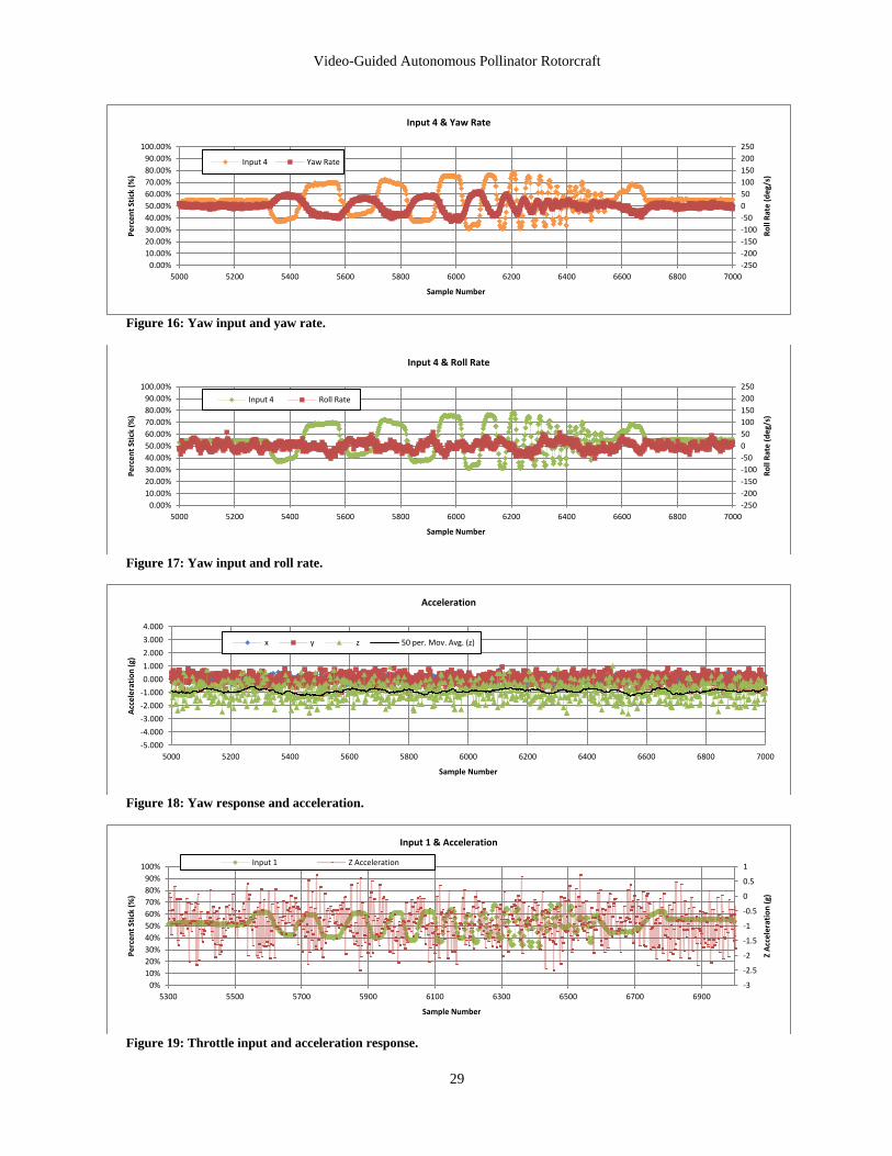
Video-Guided Autonomous Pollinator Rotorcraft
29
Figure 16: Yaw input and yaw rate.
Figure 17: Yaw input and roll rate.
Figure 18: Yaw response and acceleration.
Figure 19: Throttle input and acceleration response.
-250
-200
-150
-100
-50
0
50
100
150
200
250
0.00%
10.00%
20.00%
30.00%
40.00%
50.00%
60.00%
70.00%
80.00%
90.00%
100.00%
5000 5200 5400 5600 5800 6000 6200 6400 6600 6800 7000
Ro
ll R
ate
(d
eg/
s)
Per
cen
t St
ick
(%)
Sample Number
Input 4 & Yaw Rate
Input 4 Yaw Rate
-250
-200
-150
-100
-50
0
50
100
150
200
250
0.00%
10.00%
20.00%
30.00%
40.00%
50.00%
60.00%
70.00%
80.00%
90.00%
100.00%
5000 5200 5400 5600 5800 6000 6200 6400 6600 6800 7000
Ro
ll R
ate
(d
eg/
s)
Per
cen
t St
ick
(%)
Sample Number
Input 4 & Roll Rate
Input 4 Roll Rate
-5.000
-4.000
-3.000
-2.000
-1.000
0.000
1.000
2.000
3.000
4.000
5000 5200 5400 5600 5800 6000 6200 6400 6600 6800 7000
Acc
eler
atio
n (
g)
Sample Number
Acceleration
x y z 50 per. Mov. Avg. (z)
-3
-2.5
-2
-1.5
-1
-0.5
0
0.5
1
0%
10%
20%
30%
40%
50%
60%
70%
80%
90%
100%
5300 5500 5700 5900 6100 6300 6500 6700 6900
Z A
ccel
erat
ion
(g)
Per
cen
t St
ick
(%)
Sample Number
Input 1 & Acceleration
Input 1 Z Acceleration

Video-Guided Autonomous Pollinator Rotorcraft
30
2. Cross-Correlation
Cross-correlation is the relationship of an input control on another input control. Since the goal of system identi-
fication is to identify the effect of a primary input to another output, filtering out secondary inputs can improve the
accuracy of the analysis of the response of the primary input. CIFER has the ability to extract the cross-correlation
between a primary and a secondary input. This makes it useful as the pitch and roll input tests required some small
input from the other input due to the restricted airspace in which the tests were performed and the need to maintain
stability of the quadrotor. Conditioning the input data through MISOSA reduces the effect of the secondary input
[46]. This provides data that shows the effect of one input on an output better.
Figure 20: Cross-correlation of aileron input during elevator testing (top) and elevator input during roll testing
(above).
Figure 20 shows two cross-correlations. The upper plot shows the cross-correlation of aileron input during eleva-
tor/pitch testing, and the lower plot shows the cross-correlation of elevator input during aileron/roll testing. The
ideal test would have a coherence factor less than 0.5. There are a few frequencies that approach this threshold, such
as the low and high frequencies in the pitch test. Since the coherence averages less than .5 for most frequencies, the
data can be considered acceptable and can be used for further analysis.
3. Results
The multiple sets of the same response and sweep data are combined in CIFER and analyzed as a whole. This results
in better data. The first round of analysis obtains the Bode/coherence plots for the responses. The plots graph fre-
quency responses, phase, and coherence.

Video-Guided Autonomous Pollinator Rotorcraft
31
Figure 21: Roll, pitch, and yaw responses for roll input.
Figure 21 shows a Bode/coherence plot for roll, pitch, and yaw response with aileron input. Coherence plots
show how well the input results in an output. The coherence plot shows that the data appears most valid from .9 to
30 radians per second. Note well that high coherence also exists for pitch rate with roll input. This shows that some
off-axis coupling exists. Figure 29 in Appendix D shows a similar effect exists in roll rate response with pitch input.
However, the response has a response an order of magnitude lower than the desired response. Note that the small
amount of off-axis coupling may be a result of misalignment of the sensor to the rotorcraft flight axes.
The Bode plots for pitch, yaw, and throttle response can be found in the same appendix.
4. Roots and mathematical model
In order to obtain the numerical models of the system, the data extracted in the previous section is further post
processed. Pertinent portions of high coherence, when fed through the NAVFIT module in CIFER, provide the data
to generate the numerical models of the system responses. Figure 23 and Figure 24 show the magnitude and phase,
respectively, of roll response for roll input. The data suggests a 2nd order system with a resonant frequency around
16 rad/sec and a damping ratio of .29. The cost of the fit relates to how well the approximation fits the original data.
Costs smaller than 100 can be considered acceptable for use. The NAVFIT analysis for pitch, yaw, and throttle can
be found in Appendix E – NAVFIT results for Pitch, Yaw, and Throttle.
Table 4 summarizes the behavior for the four axes of control. Pitch and roll appear to have similar characteristics
as expected. Yaw appears to have a first-order response, while throttle appears to have a zeroth order response. Note
from Figure 31 that the throttle response has generally low coherence due to excessive accelerometer noise and a
small testing bandwidth.
The cost for the pitch data appears high due to incorporating frequencies with low coherence. By removing these
frequencies outside of the frequencies of high coherence found in Figure 29 and redoing the analysis, the data in
Table 5 shows a much smaller cost, and an increased difference up to 10 and 20 percent between the pitch and roll
modes. This may be due to different moments of inertias in the different axes or unusual control board commands.
Further research can determine the exact cause.
Table 4: Summary of poles
Mode Real component Imaginary
component
Damping
ratio
Natural frequency
(rad/sec)
Steady state
gain
Delay
(sec)
Cost
Pitch -4.143 ±14.61 .2727 15.19 1,263 .0332 102.1
Roll -4.789 ±15.72 .2913 16.44 1,449 .0282 13.66
Yaw -7.393 0.000 1.000 7.383 34.58 .0306 3.822
Throttle N/A N/A N/A N/A 99.77 -.072 38.22
Table 5: Pitch and roll poles compared with additional filtering
Pitch -3.907 ±14.19 .2654 14.72 1,186 .0265 20.88
Roll -4.789 ±15.72 .2913 16.44 1,449 .0282 13.66

Video-Guided Autonomous Pollinator Rotorcraft
32
Figure 22: Bode diagram for roll response with aileron input.
Figure 23: Roll magnitude response for roll input.
Figure 24: Roll phase for roll input.

Video-Guided Autonomous Pollinator Rotorcraft
33
5. Simulink simulation
The data obtained from the NAVFIT can be used in Simulink to perform control law analysis and controller de-
sign. Figure 25 shows a feedback loop for roll rate.
Figure 25: A roll rate feedback loop.
A step response can be generated with the lines of MATLAB code in Table 6.
Table 6: Generating a step response from a Simulink Model with MATLAB clear all; close all; clc;
[aa,bb,cc,dd] = linmod('v0_2'); P = ss(aa,bb,cc,dd); [aaa,bbb,ccc,ddd] = linmod('v0_2_2'); PD = ss(aaa,bbb,ccc,ddd); step(P,3) hold on; step(PD,3,'r--')
Figure 26 shows the results of the code and model above. The initial proportional controller shows the low
damping nature of the response with a relatively long setting time. By including a derivative gain the damping in-
creases, resulting in a shorter settling time. However, it also increases the overshoot. Lastly, a steady state error
exists due to the lack of an integrator. This may not be of concern as some roll rate is still exhibited at small propor-
tional gains. For maneuvering the quadrotor, small inputs can successfully control the platform.
6. Conclusion
Based on the results of the analysis, a few of the hypotheses can be discussed. The first hypothesis states that due
to the symmetry of the quadrotor, no off-axis coupling exists for any axis of motion. However, the Bode diagrams
for pitch and roll show that a very small amount of coupling exists for these control axes. The coupling has a value
an order of magnitude lower than the primary output response. Considering the possible error due to the lack of cali-
bration, this error can be considered negligible.
The second hypothesis states that the yaw response has no coupling on any other axis. The data shows that yaw
response has excellent yaw coherence and response. However, very low coherence to the other responses exists, so
no data can be drawn between the couplings between yaw and roll/pitch responses.
The correlation between throttle input and z-acceleration exists, but the evidence is not convincing due to the
relatively low coherence. The data suggests that some coherence exists for some frequencies, but the coherence does
not have the same caliber as the pitch, roll, and yaw data.
From the data, a control law can now be designed.
Figure 26: Step responses for roll mode with P and PD controller
p
1
Out1
Transport Delay
den(s)
1449.5
Transfer Fcn
PID(s)
PID Controller
1
In1

Video-Guided Autonomous Pollinator Rotorcraft
34
B. CMUcam4 parameter ID
To perform the parameter identification of the CMUcam4 servo controller, CIFER requires the input into camera
and the output from the servo. The following excerpts of code, written in part by P. Woodrow, gather the data re-
quired for the analysis. The Mega-based System Identification unit calls the slave Arduino with the CMUcam4
onboard for the data for recording. The tests only analyze the response in horizontal direction. The gains used incor-
porate 1000 units of ‘derivative’ gain and 50 units of ‘proportional’ gain. The tests will reveal if the gains are
mislabeled or not. It can be assumed that the vertical response has identical behavior. Further testing can confirm
this assumption.
#include <CMUcam4.h>
#include <CMUcom4.h>
#include <Wire.h>
#define SLAVE_ADDRESS 0x01 //slave address; decimal: 1
#define REG_MAP_SIZE 9 //store 3 registers; timestamp, mx, my
...
unsigned char registerMap[REG_MAP_SIZE];
unsigned long timeStamp = 0;
int tiltPos = 0;
int panPos = 0;
void setup()
{
Wire.begin(SLAVE_ADDRESS);
Wire.onRequest(requestEvent);
cam.begin();
...
cam.automaticPan(true, false); // Turn panning on.
cam.autoPanParameters(50, 1000); // Yaw gains
...
}
void loop()
{
CMUcam4_tracking_data_t data;
cam.trackColor(RED_MIN, RED_MAX, GREEN_MIN, GREEN_MAX, BLUE_MIN, BLUE_MAX);
for(;;)
{
cam.getTypeTDataPacket(&data); // Get a tracking packet.
panPos = cam.getServoPosition(0);
tiltPos = cam.getServoPosition(1);
storeData(data.mx,data.my,panPos,tiltPos);
...
}
}
void storeData(int mx, int my, int pp, int tp)
{
registerMap[0] = (int)((pp >> 8) & 0XFF);
registerMap[1] = (int)((pp & 0XFF));
registerMap[2] = (int)((tp >> 8) & 0XFF);
registerMap[3] = (int)((tp & 0XFF));
registerMap[4] = (int)((mx >> 8) & 0XFF);
registerMap[5] = (int)((mx & 0XFF));
registerMap[6] = (int)((my >> 8) & 0XFF);
registerMap[7] = (int)((my & 0XFF));
}
void requestEvent()
{
//Set the buffer to send all bytes
Wire.write(registerMap, REG_MAP_SIZE);
}

Video-Guided Autonomous Pollinator Rotorcraft
35
Figure 27: The Bode/coherence plots for the CMUcam4 servo response to the centroid location in the x direction.
After performing two sine sweeps, CIFER can then analyze the data. Figure 27 shows the resulting
bode/coherence plots show the frequency analysis of the system.
The coherence plots show that the input data, the sine sweep, has a very strong correlation to the output data, the
servo commands. The decreasing gain at 20dB/decade and the increase of 90 degree in phase suggests a zero in the
denominator and an integrator s in the denominator of the transfer function.
s a
ks
(10)
Rearranging the terms in the equation above leads to
1a
ks
(11)
ak
ks
(12)
Equation (12) shows that the controller has a proportional and integral term.
Performing a NAVFIT analysis shows that the controller can be modeled as a proportional/integral controller,
with the results shown in Figure 28. The controller has a zero at -1.54 rad/sec and an integrator at the origin. This
system has consistency with the proof above that a zero/integrator transfer function models a proportional/integral
controller. Thus, the analysis shows that the documentation for the CMUcam4 gains is incorrect for the system pro-
grammed.
This system should not be used for providing navigation, however. Since the centroid location is directly acces-
sible through the serial connection, that information should be used instead of the output signal passed through the
servo output as it is the raw data.
XII. Flight platform flight tests
A. Preliminary flight tests
The 2-D motion restraint apparatus is used to restrict the quadrotor motion to a quasi 2-D motion. It consists of a
pole placed through a hole that exists in the center of the quadrotor. The pole is attached to a pink foam base to re-
strain its motion. The system does not restrain the motion to a 2-D due to loose tolerances between the hardware
interfaces. The restraint apparatus did serve a as a safety by preventing the quadrotor from straying too far from the
center of the test area.
Before flight testing can begin, the code requires a target color inputted. Initial testing used a bright red box.
However, this method encountered serious recognition issues due to varying lighting by examining the video out
port data. Changing the target color to a bright white light source vastly improved image recognition confidence.
This yielded better response, higher confidence values, and better tracking.

Video-Guided Autonomous Pollinator Rotorcraft
36
Figure 28: Model fit for the pan servo controller
By enabling the yaw servo out signal on the CMUcam4, the yaw response can be tested. The pilot controls the
throttle, pitch, and roll angles. By moving the target around the quadrotor, the response can be observed qualitative-
ly. The quadrotor appears to take some time to respond to a step function, thus having a long setting time of about 2-
4 seconds and tends to overshoot.
Altitude control is also tested with the tilt servo out port. The signal is capable of increasing the altitude of the
quadrotor, but tends to overshoot. When the tracking is lost, the control law is programmed to cut the throttle to 45%
to facilitate a slow decent. However, the decent is still too fast and the quadrotor cannot respond in time to maintain
altitude. Thus, a better method for maintaining altitude is identified and is undergoing development.
XIII. Future work
In order for the flight system to have the necessary information to know the state of the rotorcraft, it needs a few
more sensors onboard.
Altitude can be provided with a Ping))) ultrasonic sensor. The sensor sends out an ultrasonic pulse periodically
and listens for the return of the pulse. If the pointed down towards the ground, the amount of time it takes for the
return pulse can provide altitude information. The system has a limitation on the maximum distance detectable of
approximately 3 feet. For testing purposes, this should be a sufficient altitude.
Directional information can be provided with a magnetometer. This allows the flight platform to know which di-
rection the rotorcraft is facing. This is useful in testing to maintain a certain direction for 2-d testing or
circumnavigating around a tree in 3-d testing.
A GPS unit can provide the rotorcraft with its location. Predefined areas and locations can be programmed into
the flight platform and be used to perform point to point navigation. It can also provide velocity data. However, be-

Video-Guided Autonomous Pollinator Rotorcraft
37
cause the information is not updated at high frequency, the velocity needs to be derived from accelerometer data to
obtain instantaneous velocity.
After the instrument suite is complete and integrated, the autonomous routine can be designed. The code seg-
ment below shows that inside the main loop a safety switch allows a pilot to switch between autonomous mode and
manual mode to regain control of the rotorcraft in the event that the autonomous routine does not perform as ex-
pected.
if (safety switch is off)
{do autonomous program}
else
{let pilot control rotorcraft}
The algorithm for hover flight is the most important and is currently being developed. After this, the algorithms
for motion can be developed, then, lastly, the highest level routines can be developed.
XIV. Conclusion
Phase two of the project is now complete. The flight parameters for the rotorcraft have been identified. The re-
maining work shall be on using the information gathered to develop the control laws that allow the flight computer
to perform the tasks defined in the goal of this project. Much later down the line, the code can be exported into a
miniature flying device for efficiency.
The project aims to provide support for the bee colonies. As Wood reports, it is only a short-term solution and
not a permanent fix. One day, biologists and ecologists can determine a more permanent solution to bee colony col-
lapse. Currently, researchers at the Harvard School of Engineering and Applied Science work towards developing a
highly efficient temporary solution to the problem. The main difference between Harvard’s solution and the pro-
posed solution is the focus on guidance via a live image signal instead of an idealized miniaturized flight platform.
The loss of bee pollinators poses a significant danger to nature and our culture. This project aims to provide addi-
tional research into this area of research and mitigate some of these dangers.

Video-Guided Autonomous Pollinator Rotorcraft
38
Appendix A – Cost Breakdown
The project meets its financial goals of keeping the research costs below one thousand dollars. The majority of
the cost for the flight platform comes from the CMUcam4. Future work can use wholesale prices, as well as minia-
turized components.
Table 7: A list of components and their associated costs. Miscellaneous parts include consumables required to build
the rotorcraft and other components that do not go on the rotorcraft during flight.
VGAPR BILL OF MATERIALS
Item Unit Cost Quantity Cost
Quadrotor frame and motors $ 33.95 1 $ 33.95
Propellers $ 3.83 2 $ 7.66
Arduino Uno $ 21.95 1 $ 21.95
CMUcam4 $ 103.93 1 $ 103.93
Battery $ 29.99 2 $ 59.98
MPU-6050 IMU $ 43.64 1 $ 43.64
Control board $ 19.95 1 $ 19.95
Speed controllers $ 7.22 4 $ 28.88
SEN-10530 Magnetometer $ 14.95 1 $ 14.95
Sub-total $ 334.89
Miscellaneous parts $ 161.07 1 $ 161.07
Grand total w/misc parts $ 495.96
Appendix B
Table 8: Traveling Salesman code.
clear all; close all; clc;
%% generate points randomly
rng(1); %pseudorandom control
nMax = 64; % largest dimensions
nPoints = 8; % number of points
x = randi(nMax,nPoints,1); % generate x coords
y = randi(nMax,nPoints,1); % generate y coords
figure(1);
plot(x,y,'-.or');
axis equal;
hold on;
coord = [x y]
% coord(nPoints,:) %call off this point
%% Calculate distance for a given point
i= size(coord,1);
[a]= distFromPoint(coord,i)';
%% Calculate distance between points
cost1 = cost(coord);
cost1tot = sum(cost1)
%% Switch longest leg with nearest neighbor
[maxDist,maxLeg] = max(cost1);
maxLeg
minDist = distFromPoint(coord,maxLeg);
minDist(minDist == 0) = [NaN];
[minDist,nearest] = min(minDist);
nearest
newPath = switchLeg(coord, maxLeg, nearest)
cost2 = cost(newPath);
cost2tot = sum(cost2)
Video-Guided Autonomous Pollinator Rotorcraft
39
if (cost2tot > cost1tot)
newPath=coord
end
figure(1)
plot(newPath(:,1), newPath(:,2),'-o')
axis equal;
function [ cost ] = cost( M )
%COST calculates the total distance travelled for a given path M
% It uses the Pythagorean formula.
len = size(M,1); %assume size is greater than 2
for j = 1:1:len-1
cost(j) = sqrt((M(j,1)-M(j+1,1))^2+(M(j,2)-M(j+1,2))^2);
end
cost=cost';
end
function [ y ] = distFromPoint(M,i)
%DIST calculates the distance of points in x relative to the point
% at index i
% It uses the Pythagorean formula
len = size(M,1);
for j = 1:1:len
y(j) = sqrt((M(i,1)-M(j,1))^2+(M(i,2)-M(j,2))^2);
end
function [ newCoords ] = switchLeg( coords, maxLeg, nearest )
%SWITCHLEG switches the longest leg with the nearest point
newCoords = coords;
temp = coords(nearest,:);
newCoords(nearest, :) = coords(maxLeg+1,:);
newCoords(maxLeg+1, :) = temp;
end
Appendix C
Table 9: The facial-recognition code provided by A. Huaman, with modifications in grey. Note that the two .xml files
are not included in this report. /**
* @file objectDetection2.cpp
* @author A. Huaman ( based in the classic facedetect.cpp in samples/c )
* @brief A simplified version of facedetect.cpp, show how to load a cascade classifier and how
to find objects (Face + eyes) in a video stream - Using LBP here
*/
#include "opencv2/objdetect/objdetect.hpp"
#include "opencv2/highgui/highgui.hpp"
#include "opencv2/imgproc/imgproc.hpp"
#include <iostream>
#include <stdio.h>
using namespace std;
using namespace cv;
/** Function Headers */
void detectAndDisplay( Mat frame );
/** Global variables */
String face_cascade_name = "lbpcascade_frontalface.xml";
String eyes_cascade_name = "haarcascade_eye_tree_eyeglasses.xml";
CascadeClassifier face_cascade;
CascadeClassifier eyes_cascade;
string window_name = "Capture - Face detection";
RNG rng(12345);
/**

Video-Guided Autonomous Pollinator Rotorcraft
40
* @function main
*/
int main( void )
{
CvCapture* capture;
Mat frame;
//-- 1. Load the cascade
if( !face_cascade.load( face_cascade_name ) ){ printf("--(!)Error loading 1 \n"); return -1; };
if( !eyes_cascade.load( eyes_cascade_name ) ){ printf("--(!)Error loading 2 \n"); return -1; };
//-- 2. Read the video stream
capture = cvCaptureFromCAM( 0 );
if( capture )
{
for(;;)
{
frame = cvQueryFrame( capture );
//-- 3. Apply the classifier to the frame
if( !frame.empty() )
{ detectAndDisplay( frame ); }
else
{ printf(" --(!) No captured frame -- Break!"); break; }
int c = waitKey(10);
if( (char)c == 'c' ) { return 0; }
}
}
return 0;
}
/**
* @function detectAndDisplay
*/
void detectAndDisplay( Mat frame )
{
std::vector<Rect> faces;
Mat frame_gray;
cvtColor( frame, frame_gray, CV_BGR2GRAY );
equalizeHist( frame_gray, frame_gray );
//-- Detect faces
face_cascade.detectMultiScale( frame_gray, faces, 1.1, 2, 0, Size(10, 10) );
for( size_t i = 0; i < faces.size(); i++ )
{
Mat faceROI = frame_gray( faces[i] );
std::vector<Rect> eyes;
//-- In each face, detect eyes
/* eyes_cascade.detectMultiScale( faceROI,
eyes,
1.1,
2,
0 |CV_HAAR_SCALE_IMAGE,
Size(5, 5) ); */
if( eyes.size() == 0)
{
//-- Draw the face
Point center( faces[i].x + faces[i].width/2, faces[i].y + faces[i].height/2 );
ellipse( frame,
center,
Size( faces[i].width/2, faces[i].height/2),
0,
0,
360,
Scalar( 255, 0, 0 ),
2,

Video-Guided Autonomous Pollinator Rotorcraft
41
8,
0 );
char text1[255];
sprintf(text1, "D(px) = %d", (int)faces[i].width);
putText( frame,
text1,
Point (200, 400),
FONT_HERSHEY_SIMPLEX,
1,
Scalar( 255, 255, 255 ),
2,
8,
false);
char text2[255];
sprintf(text2,
"cmd(x, y) = (%d, %d)",
(faces[i].x + faces[i].width/2 - 640/2),
-(faces[i].y + faces[i].height/2 - 480/2));
putText( frame,
text2,
Point (100, 200) ,
FONT_HERSHEY_SIMPLEX,
1,
( 255, 255, 255 ),
2,
8,
false);
/* for( size_t j = 0; j < eyes.size(); j++ )
{ //-- Draw the eyes
Point eye_center( faces[i].x + eyes[j].x + eyes[j].width/2,
faces[i].y + eyes[j].y + eyes[j].height/2 );
int radius = cvRound( (eyes[j].width + eyes[j].height)*0.25 );
circle( frame, eye_center, radius, Scalar( 255, 0, 255 ), 3, 8, 0 );
}*/
}
}
//-- Show what you got
imshow( window_name, frame );}

Video-Guided Autonomous Pollinator Rotorcraft
42
Appendix D
Figure 29: Pitch Bode/coherence plot
Figure 30: Yaw Bode/coherence plot
Figure 31: Throttle Bode/coherence plot

Video-Guided Autonomous Pollinator Rotorcraft
43
Appendix E – NAVFIT results for Pitch, Yaw, and Throttle

Video-Guided Autonomous Pollinator Rotorcraft
44

Video-Guided Autonomous Pollinator Rotorcraft
45
Acknowledgements
The author would like to thank the following people and group for making this project possible:
the committee members, Jill Borchard’s public speech class, Judith Steline, and Jerry Crofoot for their
continued support and guidance for this project;
the San Jose State chapter of AIAA for funding;
Paul Woodrow for the countless hours spent modifying his project, debugging, and mentorship;
Norio Eda for his piloting skills and donating much needed hard-to-find R/C parts;
Dhathri Somavarapu for her help with installing OpenCV;
George Fahmy for his advice on flight platform selection;
and Oreste Giusti for his assistance with data collection for the project.
Bibliography
[1] K. Flottum, "Expect to Pay More — a Lot More — for Almonds This Year," 6 February 2010. [Online].
Available: www.thedailygreen.com/environmental-news/blogs/bees/almond-prices-47020601. [Accessed 23
July 2012].
[2] Natural Resources Defence Council, "Why We Need Bees: Nature’s Tiny Workers Put Food," 2011.
[3] D. A. Sumner and B. Hayley, Bee-conomics and the Leap in Pollination Fees, Giannini Foundation of
Agricultural Economics, 2006.
[4] Harvard School of Engineering and Applied Science, "Robotic Pollinators: An Autonomous Colony of
Artificial Bees," 2009. [Online].
[5] Harvard School of Engineering and Applied Sciences, "Robobees - A Convergences of Body, Brain, and
Colony," 2012. [Online]. Available: http://robobees.seas.harvard.edu/.
[6] R. J. Wood, B. Finio, K. Ma, N. O. Perez-Arancibia, P. S. Sreetharan, H. Tanaka and J. P. Whiney,
"Progress on "pico" air vehicles," Harvard School of engineering and Applied Sciences, Cambridge, MA,
2011.
[7] MicroroboticsLab, "RoboBee altitude control," Harvard Microrobotics Lab, 20 September 2011. [Online].
Available: http://www.youtube.com/watch?v=jXo0DYxsXkU. [Accessed 18 August 2012].
[8] M. LaMonica, "RoboBees ready for mass production. Thanks, Harvard!," CNET News, 16 February 2012.
[Online]. Available: http://news.cnet.com/8301-11386_3-57379150-76/robobees-ready-for-mass-
production-thanks-harvard/. [Accessed 26 September 2012].
[9] S. Saripalli, J. F. Montgomery and G. S. Sukhatme, "Visually-Guided Landing of an Unmanned Aerial
Vehicle," IEEE Transactions on Robotics and Automation, vol. 19, no. 3, pp. 371-381, 2003.
[10] FPVFlying.com, "What is FPV Flying?," FPVFlying.com, 2012. [Online]. Available:
http://www.fpvflying.com/pages/What-is-FPV-flying%3F.html. [Accessed September 2012].
[11] Sunset Books, Sunset Western Garden Book, Menlo Park, CA: Lane Publishing Co., 1989.
[12] P. H. Raven and G. B. Johnson, "Biology - Plant Reproduction," 2001. [Online]. Available:
http://www.mhhe.com/biosci/genbio/raven6b/graphics/raven06b/other/raven06_42.pdf. [Accessed 24
October 2012].
[13] K. Sytsma, "Pollination Biology," [Online]. Available:
http://www.botany.wisc.edu/courses/botany_400/Lecture/0pdf/18Pollination.pdf. [Accessed 24 October
2012].
[14] M. Hanlon, "A bees-eye view: How insects see flowers very differently to us," Daily Mail Online, 8 August
2007. [Online]. Available: http://www.dailymail.co.uk/sciencetech/article-473897/A-bees-eye-view-How-
insects-flowers-differently-us.html#. [Accessed 26 September 2012].
[15] O. Amidi, "An Autonomous Vision-Guided Helicopter," Carnegie Mellon University, Pittsburgh, 1996.
[16] L. Mejias, S. Saripalli, P. Campoy and G. S. Sukhatme, "Visual Servoing of an Autonomous Helicopter in
Urban Areas Using Feature Tracking," 2005.
[17] G. Welch and G. Biship, "An Introduction to the Kalman Filter," SIGGRAPH, p. 45, 2001.
[18] S. Gould, J. Arfvidsson, A. Kaehler and B. Sapp, "Peripheral-Foveal Vision for Real-time Object

Video-Guided Autonomous Pollinator Rotorcraft
46
Recognition and Tracking in Video," Stanford University, Stanford, 2005.
[19] S. Saripalli, J. F. Montgomery and G. S. Sukhatme, "Vision-Based Autonomous Landing of an Unmanned
Aerial Vehicle," 2001.
[20] Y. Wantabe, E. N. Johnson and A. J. Calise, "Stochastically Optimized Monocular Vision-Based Guidance
Design," American Institute of Aeronautics and Astronautics, p. 16, 2007.
[21] CMUcam.org, "CMUcam4 Arduino Interface Library," CMUcam, 2013. [Online]. Available:
http://www.cmucam.org/docs/cmucam4/arduino_api/functions.html. [Accessed 2013].
[22] cmucam.org, "CMUcam4_tracking_data_t Struct Reference," 10 February 2013. [Online]. Available:
http://www.cmucam.org/docs/cmucam4/arduino_api/struct_c_m_ucam4__tracking__data__t.html#a5d41cf
5ef2316b748ed36ffecb4d54bd. [Accessed 2013].
[23] M. K. Kaiser, N. R. Gans and W. E. Dixon, "Vision-Based Estimation for Guidance, Navigation, and
Control of an Aerial Vehicle," IEEE Transactions on Aerospace and Electronic Systems, vol. 46, no. 3, pp.
1064-1077, 2010.
[24] D. Lowe, "Object recognition from local scale-invariant features," Proceedings of the IEEE International
Converence on Robotics and Automation, pp. 1150-1067, 2006.
[25] D. G. Lowe, "Object Recognition from Local Scale-Invariant Features," Proceedings of the International
Conference on Computer Vision, p. 8, 1999.
[26] OpenCV, "OpenCV," OpenCV, 8 May 2012. [Online]. Available: http://opencv.willowgarage.com/wiki/.
[Accessed October 2012].
[27] J. Noble, "Arduino + Servo + openCV Tutorial [openFrameworks]," 28 June 2010. [Online]. Available:
http://www.creativeapplications.net/tutorials/arduino-servo-opencv-tutorial-openframeworks/. [Accessed 8
October 2012].
[28] N. Dalal and B. Triggs, "Histograms of Oriented Gradients for Human Detection," p. 8.
[29] G. L. Barrows, "Turn your Arduino into an [sic] blazing image processing machine! (Tam2 and Tam4 chip
shields available at Centeye)," 25 February 2011. [Online]. Available:
http://embeddedeye.com/profiles/blogs/turn-your-arduino-into-an. [Accessed 31 August 2012].
[30] nootropic design, "Video Experimenter," 2012. [Online]. Available:
http://nootropicdesign.com/ve/index.html. [Accessed 24 October 2012].
[31] nootroopicdesign, "Computer Vision: Object Tracking," 15 March 2011. [Online]. Available:
http://www.youtube.com/watch?v=DIGZXcg0NIA. [Accessed 24 October 2012].
[32] J.-P. Lang, "Wiki," 2011. [Online]. Available: http://www.cmucam.org/projects/cmucam4/wiki. [Accessed
November 2012].
[33] "Arduino + OpenCV," 2009. [Online]. Available: http://arduino.cc/forum/index.php/topic,39081.0.html.
[Accessed November 2012].
[34] J.-P. Lang, "How to use the CMUcam4 properly," 2011. [Online]. Available:
http://www.cmucam.org/projects/cmucam4/wiki/How_to_use_the_CMUcam4_properly. [Accessed
December 2012].
[35] A. Huaman, objectDetection2.cpp.
[36] OpenCV/Willow Garage, "Camera Calibration and 3d Reconstruction," 2010. [Online]. Available:
http://opencv.willowgarage.com/documentation/cpp/camera_calibration_and_3d_reconstruction.html.
[Accessed November 2012].
[37] S. Swei, Interviewee, Interview with Dr. Sean Swei. [Interview]. 6 March 2013.
[38] Wolfram Research, Inc., "Traveling Salesman Problem," 2012. [Online]. Available:
http://mathworld.wolfram.com/TravelingSalesmanProblem.html. [Accessed 25 October 2012].
[39] A. Betten, "Mathematical Algorithms using Matlab, Maple, and C," 2008.
[40] G. P. Stein, O. Mano and A. Shashua, "Vision-based ACC with a Single Camera: Bounds on Range and
Range Rate Accuracy," 2000.
[41] Can_I_Trade?, "How To Read an RC Receiver With A Microcontroller - Part 1," RCArduino, 20 January
2012. [Online]. Available: http://rcarduino.blogspot.com/2012/01/how-to-read-rc-receiver-with.html.
[Accessed 2013].
Video-Guided Autonomous Pollinator Rotorcraft
47
[42] Arduino Playground, "PinChangeInt Library," Arduino.cc, 16 November 2012. [Online]. Available:
http://playground.arduino.cc/Main/PinChangeInt. [Accessed 2013].
[43] Sparkfun.com, "Triple Axis Accelerometer & Gyro Breakout - MPU-6050," Sparkfun.com, [Online].
Available: https://www.sparkfun.com/products/11028. [Accessed 2013].
[44] P. M. Woodrow, "Low Cost Flight-Test Platform to Demonstrate Flight Dynamics concepts using
Frequency-Domain System Identification Methods," (unpublished).
[45] HobbyKing.com, "Hobbyking Mini Quadcopter Frame with Motors (550mm)," 2012. [Online]. Available:
http://hobbyking.com/hobbyking/store/__19596__Hobbyking_Mini_Quadcopter_Frame_with_Motors_550
mm_.html. [Accessed 2012].
[46] CIFER, "Comprehensive Identification from Frequency Responses - User's Guide," Moffett Field, CA,
2011.
[47] O. Amidi, Y. Masaki and T. Kanade, "Research on an Autonomous Vision-Guided Helicopter," Robotics
Institute, no. 19, p. 8, 1993.
[48] A. D. Wu, E. N. Johnson and A. A. Proctor, "Vision-Aided Inertial Navigation for Flight Control," Journal
of Aerospace Computing, Information, and Communication, vol. 2, no. September, pp. 348-360, 2005.
[49] A. Casetti, E. Frontoni, A. Mancini, P. Zingaretti and S. Longhi, "A Vision-Based Guidance System for
UAV Navigation and Safe Landing Using Natural Landmarks," Journal of Intellegent and Robotic Systems,
vol. 57, pp. 234-257, 2009.
[50] F. Kendoul, K. Nonami, I. Fantoni and R. Lozano, "An Adaptive Vision-Based Autopilot for Mini Flying
Machines Guidance, Navigation, and Control," Autonomous Robots, vol. 27, p. 21, 2009.
[51] OpenCV, "Cascade Classifier," 3 November 2012. [Online]. Available:
http://docs.opencv.org/doc/tutorials/objdetect/cascade_classifier/cascade_classifier.html. [Accessed
November 2012].
[52] A. Goode, A. Rowe and K. Agyerman, "CMUcam4 Overview," CMUcam4, 2011. [Online]. Available:
http://www.cmucam.org/projects/cmucam4. [Accessed 2012].
[53] Can_I_Trade?, "Need More Interrupts To Read More RC Channels?," RCArduino, 23 March 2012.
[Online]. Available: http://rcarduino.blogspot.co.uk/2012/03/need-more-interrupts-to-read-more.html.
[Accessed 2013].