VIBRATIONS MEASURED - NASA · PDF fileVIBRATIONS MEASURED IN THE PASSENGER CABINS OF TWO JET TRANSPORT AIRCRAFT 5. Report Date August 1975 6. Performing Organization Code 7. Authorls

NAS4 TN D-7923 c.1

I

N A S A TECHNICAL NOTE

Cr)

OI N

c': n

c z

I

- A N COPY: RE L TECHNICAL

KIRTLANDiM-B. P 0-

W-

"VIBRATIONS MEASURED IN THE PASSENGER CABINS OF TWO JET TRANSPORT AIRCRAFT

John J. Catherines, John S. Mixon, I' . . ~ . .

and Hariand F. SchoM . 1 , . . .

Langley Research Center Hampton, Va. 23665

I

. .

3 N A T I O N A L AERONAUTICS AND SPACE WASHINGTON, D. C. A U G W &75 r

https://ntrs.nasa.gov/search.jsp?R=19750020964 2018-05-22T12:06:53+00:00Z

I _ . -

[ NASA TN D-7923 1. Report No. I 2. Government Accession No. T 3. Recipient's Catalog No.

4. Title and Subtitle

VIBRATIONS MEASURED I N THE PASSENGER CABINS OF TWO J E T TRANSPORT AIRCRAFT

5. Report Date August 1975

6. Performing Organization Code

7. Authorls)

John J. Catherines, John S. Mixson, and Harland F. Scholl

9. Performing Organization Name and Address

NASA Langley Research Center Hampton, Va. 23665

12. Sponsoring Agency Name and Address

National Aeronautics and Space Administration Washington, D.C. 20546

15. Supplementary Notes

8. Performing Organization Reporr No.

L-9531 10. Work Unit No.

504-09-21-01 11. Contract or Grant No.

~~

13. Type of Report and Period Covered

Technical Note -

14. Sponsoring Agency Code

I 16. Abstract

Accelerations in the lateral and vertical directions were measured at two locations on the floor of a three-jet-engine aircraft and at two locations on the floor of a two-jet-engine aircraf t dur ing a total of 13 flights each of which include6 taxiing, takeoff, ascent, cruise, descent, and landing. Accelerations over the frequency range 0 to 25 Hz were recorded continuously on magnetic tape and were synchronized with the VGH recorders in the aircraf t SO that vibratory accelerations could be correlated with the operating conditions of the a i rcraf t .

From the results it was indicated that the methodology used in segmenting the data, which were obtained in a continuous and repetitive manner, (contributes to establishing basel ine data representat ive of the f l ight characterist ics of aircraft. Significant differences among flight conditions were found to occur. The lateral accelerations were approximately 15 percent of the ver t ical accelerat ions during fl?ght but as much as 50 to 100 percent of the vertical accelerations during ground operations. The variation between the responses of the two aircraft was not statistically significant. The results also showed that more than 90 percent of the vibratory energy measured during f l ight occurred in the 0- to 3.0-Hz frequency range. Generally, the vibration amplitudes were normally distributed.

I 17. Key Words (Suggested by Author(s)) I 18. Distribution Statement

Ride quality Transpor t aircraft Vibration measurement

Unclassified - Unlimited

Subject Category 02

19. Security Classif. (of this report) 21. NO. of Pages 22. Price'

Unclassified Unclassified 54 $4.25 " -~

For sale by the National Technical Information Service, Springfield, Virginia 22161

VIBRATIONS MEASURED IN THE PASSENGER

OF TWO J E T TRANSPORT AIRCRAFT

CABINS

John J. Catherines, John S. Mixson, and Harland F. Scholl Langley Research Center

SUMMARY

As part of a program to measure ride vibrations experienced by passengers, extensive measurements were made in two jet-transport aircraft of the type widely used in commercial airline service. Vertical and lateral vibration measurements at two floor locations in each aircraft were obtained on 13 flights under conditions representative of those normally experienced by commercial airline passengers. Using continuous recordings, the vibration measurement obtained (frequency range, 0 to 25 Hz) provided a large statist ical sample of floor-vibration data for operating conditions of taxiing, takeoff, ascent, cruise, descent, and landing. The data obtained were analyzed and are presented as baseline data for use in comparative evaluations of predicted ride vibrations for new and advanced vehicles.

Ride-vibration measurements obtained indicated that for smooth cruise conditions, there were rms accelerat ions of 0.0085g and peak accelerations of less than 0.03g in the vertical direction. Other flight conditions showed rms accelerat ions of up to 0.12g and peak accelerations of 0.67g in the vertical direction. Rms lateral accelerations were about 15 percent of the vertical accelerations during flight but were as much as 50 to 100 percent of the vertical accelerations during ground operations. During flight about 90 percent of the vibratory energy was in the 0- to 3.0-Hz frequency range, compared to 60 percent during ground operations.

INTRODUCTION

In most transportation systems one source of passenger discomfort and/or ride unacceptability is the vibrations experienced by the passengers due to the motion of the vehicle in its operational mode. The concern with vibration has become more acute with the advent of high-speed ground vehicles and short takeoff and landing (STOL) aircraf t (see refs. 1 and 2). Ride quality is an important factor in public acceptance of new transportation systems and may influence their ultimate success. A need, therefore, exists for

developing ride-comfort criteria relating vibration to passenger comfort for the purpose of aiding in the design and assessment of these new modes of transportation.

Ride-comfort criteria are currently being developed using ground-based simulators (ref. 3), scheduled airline operations (ref. 4), and specially controlled aircraft (ref. 5). In order to help guide the selection of vibrations for the studies of vibration control and to aid in the assessment of the ride quality of new systems, it is useful to know the vibration characteristics of present vehicles, ranging from those smooth-riding vehicles widely accepted by the public to those judged to be less comfortable or more rough riding.

A program to measure the ride vibrations experienced by passengers has been underway since the development of a portable acceleration measurement system that could be easily used during regular passenger operations (see ref. 6). In this program, measurements have been made on a variety of transportation systems including both aircraft and surface vehicles and have been reported in the literature (refs. 6 to 10). Also, as par t of this program, extensive ride-vibration measurements were made an two jet- transport aircraft of types widely used in commercial airline service. These aircraft, which were Federal Aviation Agency (FAA) owned and piloted, were both of the fuselage- mounted engine type, one having three engines and the other two engines. Vertical and lateral vibration measurements at two floor locations in each aircraft were obtained on 13 flights in normal weather and operating under conditions representative of those that would be experienced by passengers flying in commercial airline service. Vibrations over the frequency range of 0 to 25 Hz were recorded continuously during operating conditions of taxiing, takeoff, ascent, cruise, descent, and landing. The large number of flights over a considerable distance provided a larger statist ical sample of floor-vibration data than had been obtained in the past.

The purpose of this report is to present baseline data defining the vibratory accel- e ,-ations measured on these two widely used commercial aircraft. It was thought that the vilTration environments of these two a i rc raf t a re of particular interest in view of their wide public acceptance, which indicates that the cruise of these jets represents one of the "smoothest" rides available in transportation systems today. The data in this report can be used for comparative evaluations of predicted vibrations for new and advanced vehicles.

INSTRUMENTATION

Two transducer packages and a seven-channel FM tape recorder were used to obtain the vibratory uring and recording herein.

accelerations of each aircraft. A detailed description of the meas- systems is given in reference 6, and only a brief discussion is given

2

Each transducer package contained three servoaccelerometers oriented to measure linear acceleration in three mutually perpendicular directions. The output of these packages from two locations on the aircraft was recorded on six channels of the F M tape recorder. The output f rom a marker indicator was recorded on the remaining seventh channel. The marker indicator was a three-digit, dial-set, battery-operated binary coded digital (BCD) encoder that was used to help identify flight conditions on each aircraft. A more complete description of the encoder is presented in reference 10. In addition to these measurements, flight parameters of speed and altitude were obtained from a velocity, normal acceleration, and height (VGH) recorder in conjunction with the F M tape recorder. The VGH recorder is described in reference 11. A pushbutton marker device was incorporated with the VGH recorder and, together with the three- digit encoder used with the FM tape recorder, the data were recorded with sufficient identFfication to insure good correlation between the two recorders. Figure 1 shows a typical instrumentation setup as photographed on one of the conventional takeoff and landing (CTOL) aircraft.

PROCEDURE

Field Test

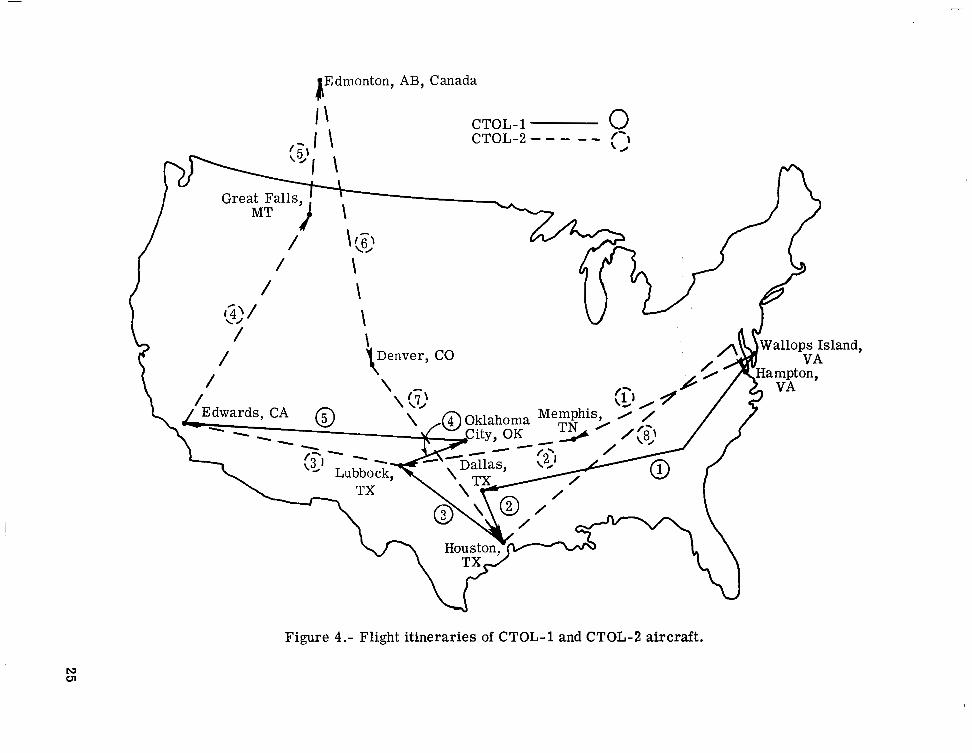
The data were obtained on FAA owned and operated aircraft during a joint FAA/USAF/NASA Runway Research Program to investigate methods for measuring runway slipperiness and aircraft performance on slippery runways. Photographs of the aircraft which are designated CTOL-1 (three engine) and CTOL-2 (two engine) a r e shown in figures 2 and 3 . Specifications for the aircraft are given in table I and were obtained from reference 12. In this program, the aircraft were flown to six or more different commercial airports in the United States and Canada as indicated by the flight itineraries shown in figure 4 . The flight procedures were similar to those used by commercial air- lines and thus provided an opportunity to obtain useful baseline vibration measurements at floor locations in the aircraft.

Baseline measurements are defined as those measurements obtained in a repetitive manner on a specific vehicle which do not exhibit much variation during a particular flight condition. These data are then considered typical for a given aircraft.

The accelerometer packages were placed at two floor locations within the passenger compartment of each aircraft: (1) behind the pilot compartment bulkhead, in front of the first row of seats, and (2) approximately at the center of gravity (c.g.) of each aircraft . Both instrument packages were bolted in place to 1/2-inch steel plates which were fitted to the seat t racks of the aircraft. The packages were oriented to measure accelerations parallel to the cabin floor in the longitudinal and side-to-side directions and perpendicular

3

to the cabin floor. These measurements are referred to herein as longitudinal, lateral, and vertical accelerations, respectively. The VGH recorder operated at a speed of 0.02 cm/sec (0.008 in/sec) continuously during the flight phase of travel between airports, including takeoffs and landings. The VGH recorder was keyed to the vibration measurements by means of the manually operated pushbutton marker shown in figure 1. Holding the marker switch down activated a bright light beam which exposed a narrow section of VGH record; for example, an 0.20-cm (0.08-in.) section of the VGH record would be exposed by holding down the pushbutton switch on the marker for a period of 10 seconds.

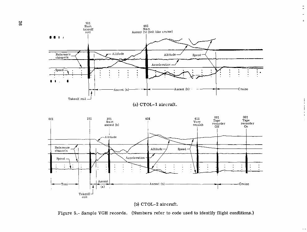
The procedure for obtaining identifiable data involved simultaneously triggering the three-digit, dial-set encoder and the pushbutton VGH marker. In this manner, the acceleration measurements were correlated with the flight parameters of velocity and altitude. Sample VGH records are shown in figure 5. The altitude and speed traces can be seen to be varying with the flight condition of the aircraft, and the marker signals are indicated. The numbers of the marker signals are those encoded on the FM tape recorder. Marker No. 401 was made when the observer felt that the aircraft had reached the smooth cruise condition characterized by low noise and vibration.

The basic data were collected in the form of FM tape recordings of the instantaneous values of the three linear accelerations for each of the two measurement boxes and paper recordings of the VGH data such as shown in figure 5. The FM tape recorder was turned on before the aircraft began to taxi and was usually left on to record continuously until the a i rcraf t had come to a stop following taxiing at the completion of that flight. In some of the longer flights, the tape recorder was turned off during part of the smooth cruise; however, the VGH recorder was always on during the complete flight.

Data Analysis

The first step in the analysis of the data was to obtain oscillographic time histories of the FM tape-recorded accelerations, VGH records, and other flight information relating to the flight cycle of the aircraft. Using this information, the flight cycle was divided into 10 reasonably well-defined conditions as discussed herein.

The flight conditions used in this report are defined in table II, the duration of each condition is presented in table 111, and the aircraft operating parameters are shown in table IV. The details of how each condition was defined will be briefly discussed with the aid of figure 5, showing sample VGH records, which are divided into segments according to the flight conditions of the aircraft . The first segment is the taxi condition as shown by a noticeable change in the magnitude of the acceleration on the VGH trace of figure 5(b). Also, postlanding segments were included as par t of the taxi condition. The second segment is 'the takeoff condition, the onset of which was indicated by a marker put on the tape

4

and VGH recorders at the beginning of the forward motion of the aircraft, and the offset of which was indicated by a noticeable change in the frequency and magnitude of the acceleration trace as observed from the oscillograph record. The portion of flight between takeoff and constant-altitude cruise was divided into an ascent (a) and an ascent (b) flight condition. It should be noted that different methods were used to define the ascent conditions for the CTOL-1 and the CTOL-2 aircraft. For the CTOL- 1, the ascent (a) condition extended from wheels-up to the time in the flight at which the observer determined that the aircraft had reached the cruise condition at which the accelerations were very low fo r a good length of time, and a code such as No. 401 in figure 5(a) was put on the tape along with a marker on the VGH record. A s shown in tables III and W, this condition lasted about 6 minutes, ending at an altitude of about 3.35 km (11 000 ft) with fairly small variation from one flight to another. The ascent (b) condition extended from the time it was thought that cruise began, as indicated by the marker such as No. 401 in figure 5(a), to the time that constant-altitude cruise actually began as indicated by the altitude trace of the VGH recorder. A s suggested by figure 5, the actual cruise condition always began later than it was felt to begin. For the CTOL-2 aircraft the ascent (a) condition ended at the point where large accelerations experienced immediately after takeoff and visible on the time-history record decreased significantly, marked as point 301 in figure 5(b). This condition suggests that some change of the environment or operation of these aircraft occurs that causes a noticeable change in the vibration at this t ime during liftoff. A s a result, the ascent (a) condition was much shorter and more variable for the CTOL-2 aircraft (see table III). The ascent (b) condition for the CTOL-2 aircraft extended from the end of the high acceleration, point 301 in figure 5(b), to the constant-altitude cruise condition. During constant-altitude cruise, rough and smooth cruise conditions were selected; that is, sample data were chosen to represent rough and smooth conditions. In the approach segment, the vibrations were also observed to be larger at lower altitudes, so approach w a s subdivided further into a smooth-segment (descent (b)) condition and a rough-segment (descent (c)) condition on the basis of the accelerations appearing on the time-history traces of the flight cycles. In addition to these two segments, a descent (a) condition extended from constant altitude to touchdown which included both descent (b) and descent (c) conditions. This method was used for both aircraft. Touchdown extended from the time just at touchdown impact indicated by a marker that was imparted to the tape and to the VGH recorder to the time that the accelerations showed a noticeable decrease, which occurred approximately 1 minute or less after touchdown impact. This segmentation of lengthy continuous tape recordings facilitated data-reduction requirements as well as provided for adequate means to define qualitatively the different phases of flight.

5

L

With the flight cycles each divided into flight conditions as described above, the next step was to analyze the data. The portion of the record analyzed is refer red to as a "run." The procedure was to digitize the tape-recorded data and then to utilize the Langley time-series-analysis computer program (ref. 13) to calculate the statistical parameters that define the characteristics of the vibration measurements. It should be noted that the mean values of acceleration were subtracted from the data.

RESULTS AND DISCUSSION

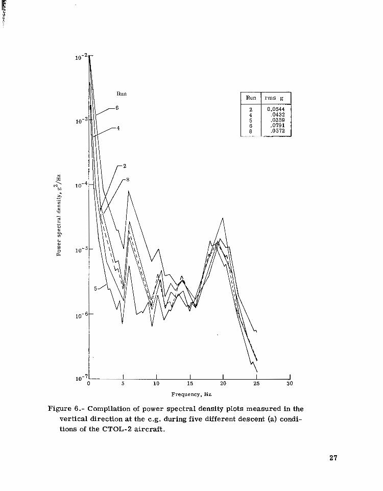
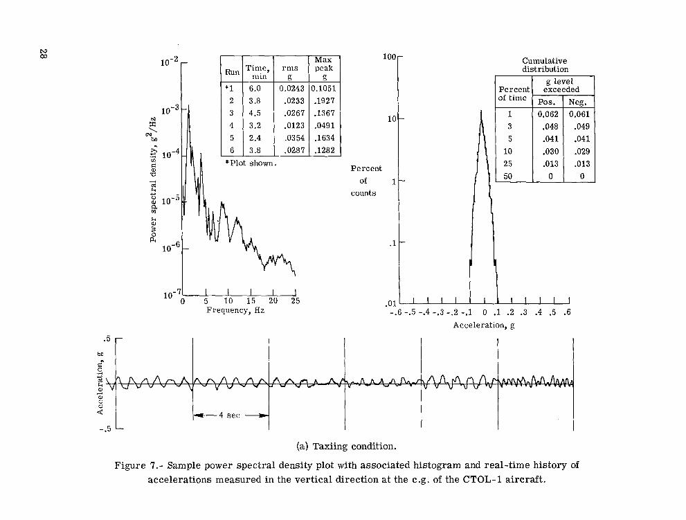
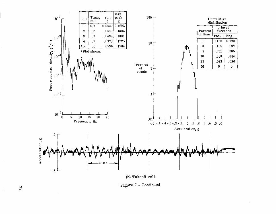
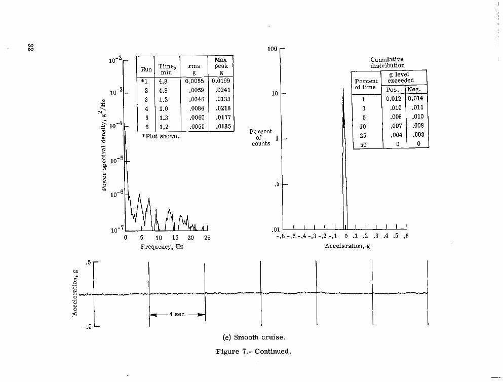
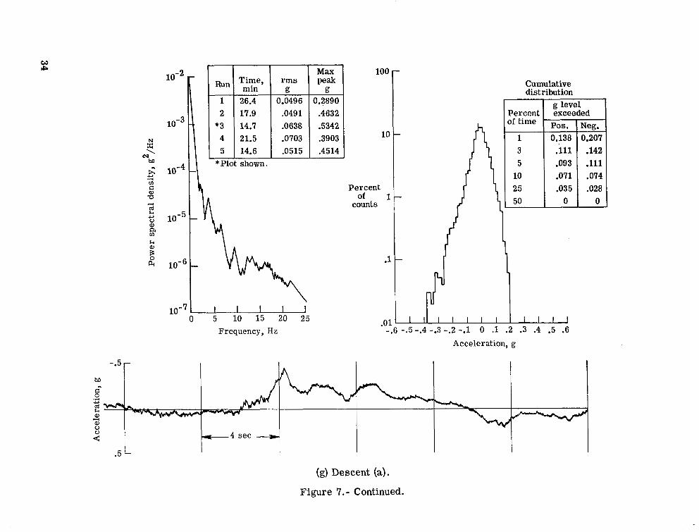
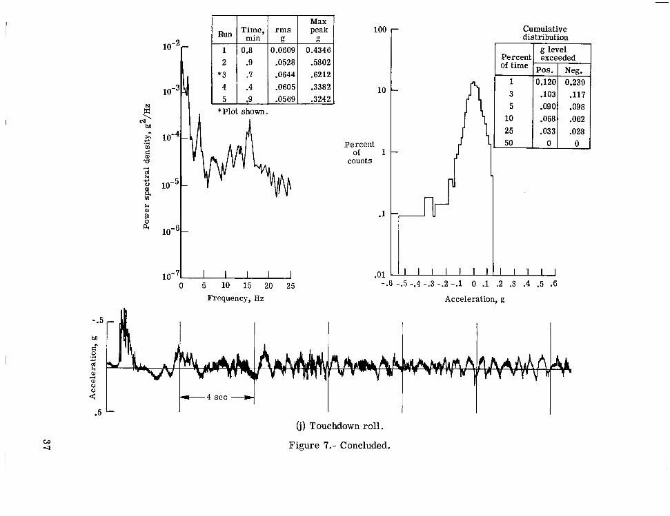
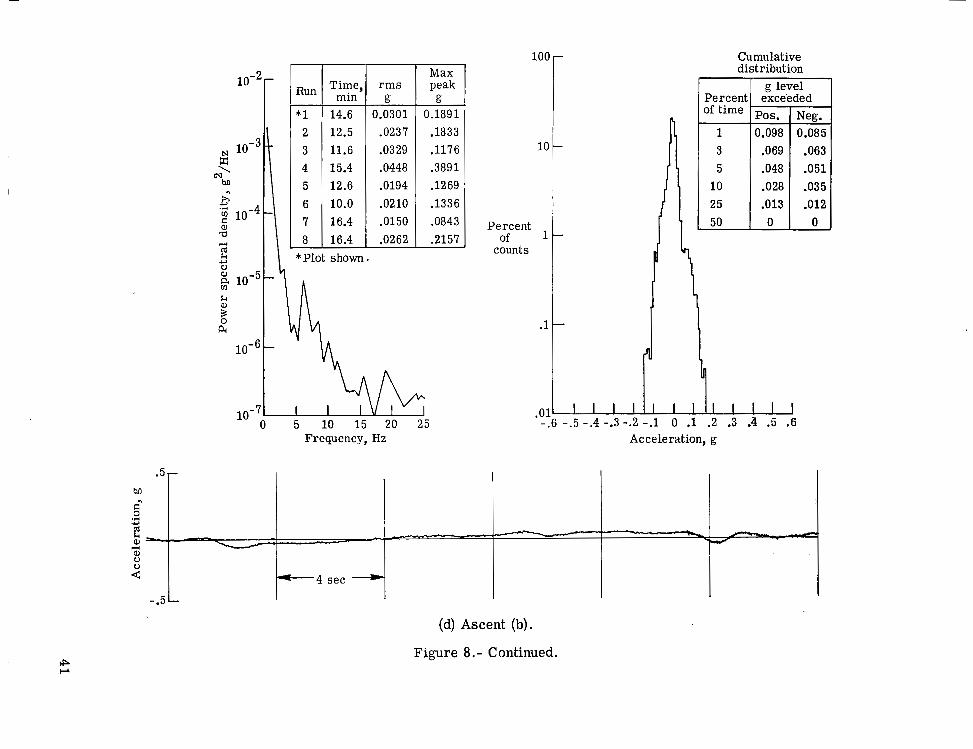
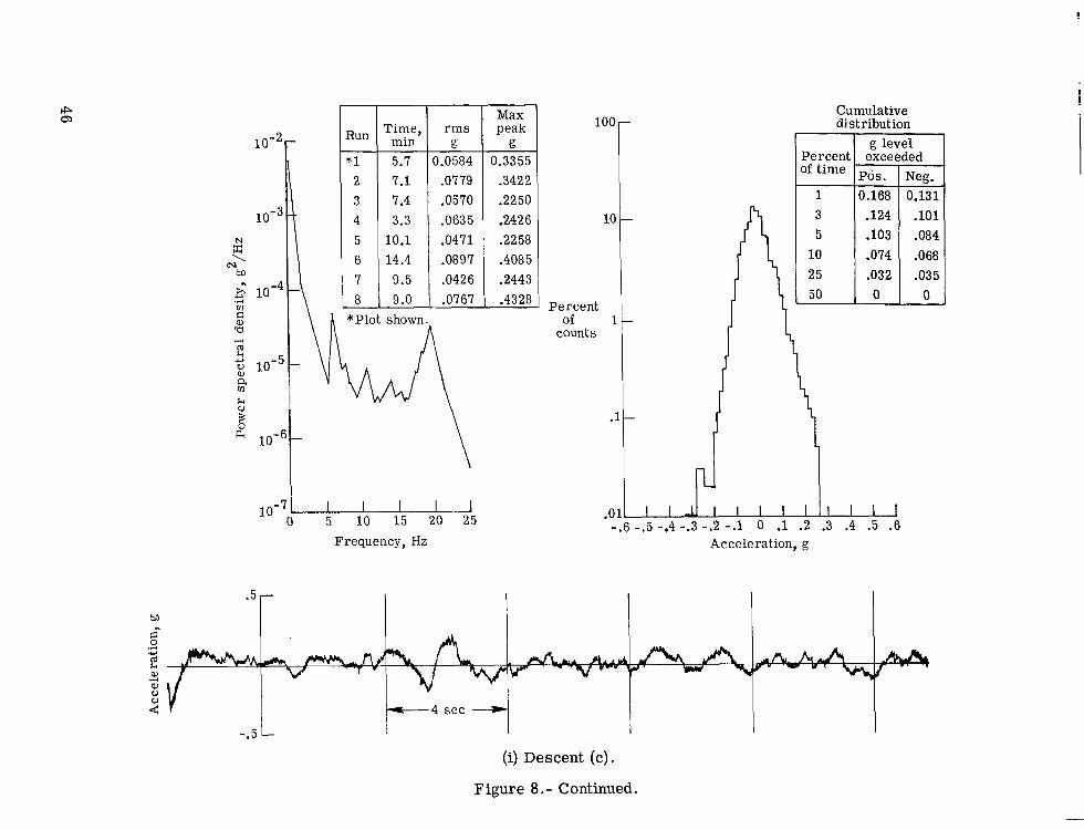
The quantity of test data that resulted from this study, as measured by the hours of tape recordings and the number of different segmented runs, was substantial, but the fact that the tests were performed essentially in a repetitive manner helped reduce the amount of data presentation. The term "baseline data" is derived from the concept of condensing the data, particularly if little variation occurs between different runs of a specific flight condition. For example, by comparing the power spectral density (PSD) plots for several runs of the descent (a) condition of the CTOL-2 aircraft as shown in figure 6, it was observed that the spectra had similar characterist ics; that is, the peaks occurred at approximately the same frequencies with usually about the same relative magnitudes, In order to simplify the data presentation, therefore, the PSD plot of one of the runs was chosen as a sample. The plot was selected to represent the mean or average PSD plot and/or corresponding rms value, which in this case was run no. 2. It may be observed that both the PSD plot and the r m s value for run no. 2 approximate the average data shown for all of the different runs. The data presented for each aircraft consist of selected PSD plots, together with the corresponding histograms (amplitude distributions), "exceedance" tables, and acceleration time histories. The data for the CTOL-1 and CTOL-2 aircraft are shown in f igures 7 and 8, respectively. Also included in these figures are tables of the rrns acceleration, the maximum or peak acceleration, and the time (in minutes) denoting the length of the analysis for each run. The run numbers, for the most part, correspond to the flight numbers shown in figure 4 and listed in table III. (This rule does not apply to the cruise condition where the cruise segments were selected at large.) The cumulative distribution tables which were derived by integrating the histograms show the percentage of time that a given acceleration level is exceeded.

Except where indicated, the data presented herein were measured in the vertical direction. It should be noted that acceleration levels measured in the lateral and, in particular, in the longitudinal directions were significantly smaller than those measured in the vertical direction. The acceleration measurements in the longitudinal direction, therefore, are not presented and only some data in the lateral direct ions are given.

6

Ftms and Peak Accelerations

The measured accelerations are indicated in figures 9 and 10, where rms acceleration and peak acceleration are charted for each flight condition for each aircraft. The data represent measurements obtained at the c.g. position and also at the forward position of the aircraft. As expected, these figures show that the smooth-cruise condition is by far the smoothest part of the flight, with rms acce lera t ions less than 0.0085g and maximum peak accelerations of 0.03g. In addition, the higher-altitude flight segments, ascent (b), rough cruise, and descent (b), are shown to have generally lower values of acceleration than the lower-altitude segments, ascent (a), and descent (c). With the exception of the smooth-cruise conditions, no other condition stands out as having accelerations that are markedly higher or lower than all other segments. R m s accelerations up to 0.12g and maximum peak accelerations of 0.67g measured during the touchdown condition are shown in these figures. Also, it can be seen that the peak g acceleration values shown in figure 10 generally conform to the overall contour displayed by the rms acce l - eration values shown in figure 9.

The accelerations shown in figures 9 and 10, when combined with other features such as frequency and seat characteristics (refs. 14 and 15), may be large enough to cause some discomfort. The two airplanes used in these tests, however, are known to be quite comfortable, both from individual passenger reaction and from wide passenger acceptance. This observation serves to emphasize the importance of such features as duration, spectrum, and amplitude distribution, as well as r m s and peak accelerations in determining the subjective response to a given vibration environment.

An attempt w a s made to establish the consistency of the acceleration measurements recorded for each successive flight condition within a given flight, that is, to determine whether large accelerations occurring during ascent (a) were followed by large accelerations during the subsequent conditions of the flight, as might be expected if accelerations were associated with pilot handling characteristics and/or weather influence. Compari- son of accelerations for various flight conditions for each flight cycle showed that the acceleration measurements did not follow a pattern but occurred randomly.

Comparison of data for two locations.- As observed in figures 9 and 10, acceleration measurements were obtained simultaneously at two locations within the passenger compartments of the aircraft . Comparison of the data for the two locations showed that the measurements were consistent for each aircraft, each acceleration measure (rms and peak), and each flight condition. For example, the lowest acceleration at the c.g. was measured on the run with the lowest acceleration at the forward position, the next highest g (c.g.) with the next highest g (forward position), and so on. In only a few cases did this relation not hold for the data shown in f igures 9 and 10.

7

Figure 11 shows the average values of the vertical rms accelerations calculated fo r all of the runs in each flight condition as measured at the two locations and for both aircraft. Examination of this figure shows that the c.g. position exhibits less rrns accelerations than the front position when the aircraft are on the ground. When the aircraft are airborne, however, the c.g. position shows higher acceleration levels than the front position.

A statistical study was performed with these data in order to establish the significance of this conclusion. A t-test (ref. 16) was used to determine the significance of the difference between paired rrns acceleration averages; that is, the difference between the averages of the rms accelerations measured simultaneously at the forward and c.g. positions of the aircraft involving all of the runs in each of the flight conditions in which the aircraf t were a i rborne. A t-value of 10.3 with 32 degrees of freedom and a t-value of 8.5 with 53 degrees of freedom were calculated for the CTOL-1 and CTOL-2 aircraft, respectively. These data allow a level of significance of less than 0.005. The result of this analysis shows that the c.g. location consistently showed more vibrational energy than the front of the aircraft in flight. It should be noted that measurements were not obtained along the whole length of the fuselage where the accelerations may change depending on the location at which the measurement is made within the aircraft, since local resonances and/or pitching motions may have an effect.

Comparison of accelerations measured on the two aircraft.- Generally, as figures 9 and 10 show, the two aircraft exhibited similar responses within the segmented flight conditions. The data appear to be grouped in accordance with the particular flight condition rather than for a particular aircraft . The statistical methods of analysis of variance were employed to demonstrate the validity of this observation. The method involved a statistical analysis for comparing the variability and differences between the rrns acceleration measurements obtained at the c.g. of the two aircraft. The computations for the analysis are summarized in the variance table shown in table V. The data given in the column of the sum of squares for each of the different flight conditions were obtained by well-established statistical formulas (see ref. 16). A brief explanation of the values presented is given in the appendix. The test shows that the vibration differences in terms of the means of the rms acceleration measurements obtained on the two a i rc raf t for all flight conditions are not significant. This result implies that, so far as these data for the rms accelerat ions are concerned, the variation between the measurements for the two aircraft obtained during each of 10 different flight conditions is no larger than would be expected by chance. It should be noted, however, that the flight conditions of "ascent (a)" and "ascent (b)" show some significance about the 5-percent level, as compared with the 25-percent probability level shown for the other flight conditions. This difference may be explained by the fact that the "ascent (a)" and "ascent (b)" flight conditions were specified

~ - ~- ~~

8

differently during the segmentation of the data between the two aircraft. As noted, the cutoff altitude for the ascent (a) flight condition for the CTOL-1 aircraft was approximately 3.35 km (11 000 ft) as compared to 1.98 km (6500 ft) for the CTOL-2 aircraf t - the altitude specified for the ascent (b) flight condition varied accordingly.

Vertical against lateral responses.- The acceleration measurements in the lateral direction for various phases of flight were generally ,considerably lower than those measured in the vertical direction. To show this relation, rms acceleration values measured at the center of gravity in the vertical and lateral directions for the CTOL-2 aircraft during the various flight conditions are shown in figure 12. A solid line has been drawn separating the airborne and the on-ground data. It should be noted that while airborne the aircraft exhibits considerably less response in the lateral direction than in the vertical direction. A statistical analysis was performed using the data shown in figure 12 to determine the linear correlation of the two variables, vertical rms acceleration and lateral rms acceleration. Correlation coefficients of 0.08 and 0.59 were calculated with the data combined when the aircraft was on the ground and airborne, respectively. Fig- u re 12 also shows that the accelerations are uncorrelated when the aircraft is on the ground and are correlated when the aircraft is airborne. The lateral response increases fractionally with increased vertical acceleration as the smooth-cruise flight condition is compared with the ascent (a) flight condition. Visually fitting a straight line (dashed line) through the "airborne" data and passing through zero suggests that the lateral acceleration is about 15 percent of the vertical acceleration, regardless of flight condition. Fo r the "on-ground" conditions, however, figure 12 shows that most of the lateral rms accelerations lie roughly between 0.0125g and O.O3g, without any dependence on the vertical acceleration.

Power Spectra

For the most par t , th is general d iscussion of the results has been concerned with the magnitude of accelerations, such as r m s and peak values. An important component in describing vibration is the frequency content of the data, that is, at what frequency do the vibrations occur. This is a very important point when describing vibrating ride environments in reference to human comfort. For example, Goldman (ref. 17) compiled equal vibration-sensation contours in terms of peak acceleration as a function of frequency, and his data show that a knowledge of frequency is essential in determining human response. For this reason, power-spectral-density analysis was utilized to identify the dominant frequencies of the aircraft motions.

Referring to the PSD plots shown in figures 7 and 8, considerable low-frequency energy is shown, with energy levels at the higher frequencies being lower by an o rder of

9

magnitude and greater. This situation was further explored by investigating the low- frequency range relative to the total range. This study was accomplished by comparing the rms acceleration level of the integrated area over the 0- to 3.0-Hz frequency range (a significant amount of energy appeared concentrated below 3.0 Hz) to the total rms acceleration value determined for the entire frequency range of 0 to 25 Hz. A s noted previously, the mean value has been subtracted from the data so that, when the frequency range is given from zero, an infinitesimal value of frequency, somewhat greater than zero, is actually implied. The vibratory energy within the 0- to 3.0-Hz frequency range as compared to the total energy over the entire frequency range (0 to 25 Hz) is shown in figure 13 on a percentage basis. This value was determined for all of the runs involving the two aircraft and, for this reason, a range of values is shown in figure 13. Examina- tion of this figure shows that a significant amount of the energy of the vibratory ride environment measured on the aircraft occurs in the low-frequency range of 0 to 3.0 Hz. When the aircraft are airborne the percentage of energy within the 0- to 3.0-Hz frequency range is usually above 90 percent with only a few values as low as 68 percent, while on the ground the percentage was lower, with most values below 70 percent and only a few as high as 95 percent. This result indicates that the responses associated with the higher frequencies (greater than 3.0 Hz) contribute more when the aircraft are on the ground than when they are in the air. A quick glance at figures 7 and 8, par t s (a), (b), and ( j ) , shows that the energy at the higher frequencies is considerably larger when the aircraft are on the ground. The arrows, shown in figure 13, signify the mean values of the percentages obtained from all the runs within each flight condition for each aircraft. It should be noted that the percentages shown for the smooth-cruise condition were somewhat lower (80 percent) than for the other airborne conditions. This situation resulted from the use of exceedingly small numbers in computing the percentage values. The accelerations are so small, especially above 3.0 Hz, that it is possible that low signal-to- noise ratio has degraded the accuracy of the measurement and caused the low percentage values shown in figure 13.

PSD comparison of CTOL-1 and CTOL-2 aircraft.- The magnitudes of the r m s and peak acceleration responses discussed previously in figures 9 to 11 indicated comparable response characteristics for each of the flight conditions investigated. Also, the energy of the vibratory motion measured on both aircraf t occurs in the low frequency band of 0 to 3.0 Hz (see figs. 7 and 8). Considerable energy is shown to occur a t higher frequencies (greater than 3.0 Hz) when the a i rcraf t are on the ground, however, but it should be noted that the ordinate scale used in presenting the PSD data is logarithmic and, therefore, the higher frequency responses appear to be magnified by o rde r s of magnitude. A more realistic observation of high-frequency content can be seen in the real-time t races shown in figures 7 and 8, where the high-frequency data are superimposed on the low -f requency data.

On the ground the suspension frequencies of the aircraft are excited as the aircraft rolls on the runway and accelerations caused by runway roughness are transmitted through the structure into the passenger compartment. This result can be seen in fig- u r e s 7(a) and 8(a), during the aircraft taxiing condition in which suspension frequencies of 1.5 Hz and 1.8 Hz are measured for the CTOL-1 and CTOL-2 aircraft, respectively. The second major response peaks shown in the PSD plots of figures 7(a) and 8(a) occur at approximately 4.3 Hz and 6.0 Hz, respectively. These frequencies most probably represent structural and/or engine-excited resonances, inasmuch as they reappear during each of the remaining flight conditions. Figure 13 shows that the mean value of the energy percentage ratio is lower for the CTOL-2 aircraft than for the CTOL-1 aircraft during ground conditions. This relationship indicates that the CTOL-2 has more energy than the CTOL-1 at frequencies above 3.0 Hz, during which passengers may be more sensitive to vertical vibration (see ref. 18). In order to assess accurately the importance to passengers of the differences between aircraft observed in figure 13, however, controlled tests with passenger subjects would be required.

Vertical and lateral spectra.- It has been previously noted that the accelerations measured in the lateral direction were appreciably smaller than those obtained in the vertical direction when the aircraft were airborne but increased substantially when the aircraf t were on the ground. An example of the data measured when the CTOL-2 aircraft was on the ground is shown in figure 14 in a PSD form. Vertical and lateral acceleration responses measured at the same time during taxiing, takeoff, and touchdown flight conditions are shown in this figure. It should be noticed that the measurements in the lateral direction are somewhat lower than those in the vertical direction and, in particular, that they do not coincide well at the low frequencies, below 5.0 Hz. At frequencies above 5.0 Hz, the dominant peak responses in the lateral direction are shown to occur at the same frequencies as the peaks of the vertical motion but with less amplitude. The differences at frequencies below 5.0 Hz are probably caused by factors such as different suspension-system characteristics for vertical and lateral directions and control by the pilot as he steered the aircraft.

Histogram Data

The histogram data which are plotted on logarithmic scales showing the distribution of instantaneous acceleration magnitudes, in percent of count, are presented in figures 7 and 8. Each level of the histogram represents the percentage of acceleration counts occurring within the acceleration interval. For the most part, these plots indicate high probability density about the mean values, which is indicative of a random process. As noted earlier, the mean values of acceleration were subtracted from the data. The cumulative distribution showing values of lfg-level exceeded" with each corresponding

11

3

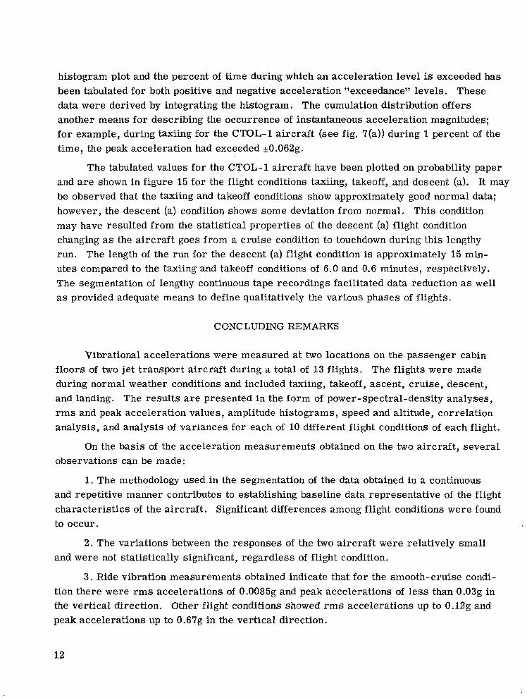
histogram plot and the percent of time during which an acceleration level is exceeded has been tabulated for both positive and negative acceleration "exceedance" levels. These data were derived by integrating the histogram. The cumulation distribution offers another means for describing the occurrence of instantaneous acceleration magnitudes; for example, during taxiing for the CTOL-1 aircraft (see fig. ?(a)) during 1 percent of the time, the peak acceleration had exceeded *O.O62g.

The tabulated values for the CTOL-1 aircraft have been plotted on probability paper and are shown in figure 15 for the flight conditions taxiing, takeoff, and descent (a). It may be observed that the taxiing and takeoff conditions show approximately good normal data; however, the descent (a) condition shows some deviation from normal. This condition may have resulted from the statistical properties of the descent (a) flight condition changing as the aircraft goes from a cruise condition to touchdown during this lengthy run. The length of the run for the descent (a) flight condition is approximately 15 minutes compared to the taxiing and takeoff conditions of 6.0 and 0.6 minutes, respectively. The segmentation of lengthy continuous tape recordings facilitated data reduction as well as provided adequate means to define qualitatively the various phases of flights.

CONCLUDING REMARKS

Vibrational accelerations were measured at two locations on the passenger cabin floors of two jet transport aircraft during a total of 13 flights. The flights were made during normal weather conditions and included taxiing, takeoff, ascent, cruise, descent, and landing. The results are presented in the form of power-spectral-density analyses, r m s and peak acceleration values, amplitude histograms, speed and altitude, correlation analysis, and analysis of variances for each of 10 different flight conditions of each flight.

On the basis of the acceleration measurements obtained on the two aircraf t , several observations can be made:

1. The methodology used in the segmentation of the data obtained in a continuous and repetitive manner contributes to establishing baseline data representative of the flight characterist ics of the aircraft. Significant differences among flight conditions were found to occur.

2. The variations between the responses of the two aircraft were relatively small and were not statistically significant, regardless of flight condition.

3. Ride vibration measurements obtained indicate that for the smooth-cruise condi- t ion there were rms accelerations of 0.0085g and peak accelerations of less than 0.03g in the vertical direction. Other flight conditions showed rms accelerations up to 0.12g and peak accelerations up to 0.67g in the vertical direction.

12

4. The lateral accelerations were approximately 15 percent of the vertical accelerations during flight, but as much as from 50 to 100 percent during ground operations.

5. Consistently, more vibratory energy was indicated at the center of gravity of each aircraft than at the front of the aircraft during flight, and less energy was indicated at the center of gravity during ground operations.

6. It was found that more than 90 percent of the vibratory energy measured during flight occurred in the 0- to 3.0-Hz frequency range, compared to about 60 percent during ground operations.

7. Generally, it was found that the acceleration amplitudes were normally distributed.

Langley Research Center, National Aeronautics and Space Administration,

Hampton, Va., May 16, 1975.

13

APPENDIX

ANALYSIS OF VAFUANCE

The procedure used for evaluating the significance of the duference between the rms accelerat ion measurements for the two aircraft is given herein. A statistical method involving the F-test (see ref. 16) which is based on an analysis of variance of the data was used. An explanation of table V will assist in describing the method.

The between aircraft sum of squares is a measure of the variation of the means of the rms acceleration values obtained for each aircraft about the overall means obtained f rom all of the rms acceleration values measured on both aircraft for a given flight condition. The within aircraft sum of squares is a measure of the variation of the r m s acceleration values within each set of data about their own group means (or may be considered as a measure of the random variability within the measurements). Since the variance between aircraft means was based upon the deviations of each of two aircraf t means from the grand or overall mean, only one degree of freedom is present (d.f. = (N - 1)). Variations within aircraft involved the deviations N1 values from their own mean and N2 values from their own mean, so the degree of freedom varied accordingly to the following formula:

d.f. = (N1 - 1) + (Nz - 1)

where NN is the number of rms acceleration values within each set of data for the CTOL-1 and the CTOL-2 a i rc raf t at a given flight condition.

When each of these sum of squares is divided by its appropriate number of degrees of freedom, two independent estimates of variance are obtained, namely, the estimated variance between aircraft means and the estimated variance within sets of data for each aircraf t at a given flight condition. The ratio of these two estimates is termed the F-ratio. If there is no significant difference between the aircraft, on the average, the F-ratio should be 1.00. If the estimated variance between aircraft means is larger than the estimated variance within the group of data, however, then the F-ratio should be greater than 1.00. The final column of data was obtained from the standard tables of F-distribution and shows what the probability is that the calculated F-ratios could have occurred by chance, in percent.

14

REFERENCES

1. Ullman, Kenneth B.; and O'Sullivan, William B.: The Effect of Track Geometry on Ride Quality. Paper No. 69 C P 355-1EA, Inst. Elec. & Electron. Eng., Apr. 1969.

2. Kuhlthau, A. R.; and Jacobson, I. D.: Analysis of Passenger Acceptance of Commer- cial Flights Having Characteristics Similar to STOL. STOL Program Tech. Rep. 403208 (Grant NGR-47-005-181), Univ. of Virginia, Mar. 1973. (Available as NASA CR-132285.)

3. Clevenson, Sherman A.; and Leatherwood, Jack D.: On the Development of Passenger Vibration Ride Acceptance Criteria. Shock & Vib. Bull., Bull. 43, Pt. 3, U S . Dep. Def., June 1973, pp. 105-111.

4. Kuhlthau, A. R.; and Jacobson, Ira D.:, Investigation of Traveler Acceptance Factors in Short-Haul Air Carrier Operations. Symposium on Vehicle Ride Quality, NASA TM X-2620, 1972, pp. 211-228.

5. Seckel, Edward; and Miller, George E .: Exploratory Flight Investigation of Ride Quality in Simulated STOL Environment. Symposium on Vehicle Ride Quality, NASA TM X-2620, 1972, pp. 67-89.

6. Catherines, John J.; Clevenson, Sherman A.; and Scholl, Harland F.: A Method for the Measurement and Analysis for Ride Vibrations of Transportation Systems. NASA TN D-6785, 1972.

7. Catherines, John J.: Measured Vibration Ride Environment of a STOL Aircraft and a High-speed Train. Shock & Vib. Bull., Bull. 40, Pt. 6, U.S. Dep. Def., Dec. 1969, pp. 91-97.

8. Catherines, John J.; and Clevenson, Sherman A.: Measurements and Analysis of Vibration Ride Environments. Preprint No. SW-70-21, Amer. Helicopter SOC., Nov. 1970.

9. Conner, D. William: Ride Quality - An Increasingly Important Factor in Transporta- tion Systems. Paper presented at 1971 International IEEE Conference on Systems, Networks, and Computers (Oaxtepec, Mexico), Jan. 1971.

10. Clevenson, Sherman A.; and Catherines, John J.: Measurement and Analysis of Vibra- tion in Transportation Systems. Volume 26 of AAS Science and Technology Series, F. W. Forbes and P. Dergarabedian, eds., Amer. Astronaut. SOC., c.1971, pp. 197-202.

11. Richardson, Norman R.: NACA VGH Recorder. NACA TN-2265, 1951.

12. Taylor, John W. R., ed.: Jane's All the World's Aircraft, 1973-1974. McGraw-Hill Book Co., Inc., c.1973.

13. Ward, Robert C.: Dynamic Data Analysis Techniques Used in the Langley Time Series Analysis Computer Program. NASA TM X-2160, 1971.

14. Leatherwood, Jack D.: Vibrations Transmitted to Human Subjects Through Passenger Seats and Considerations of Passenger Comfort. NASA TN D-7929, 1975.

15. Hanes, R. M.: Human Sensitivity to Whole-Body Vibration in Urban Transportation Systems: A Literature Review. APL/JHU-TPR 004, Johns Hopkins Univ., May 1970.

16. Bruning, James L.; and Kintz, B. L.: Computational Handbook of Statistics. Scott, Foresman and Co., c.1968.

17. Goldman, David E.; and Von Gierke, Henning E.: Effects of Shock and Vibration on Man. Engineering Design and Environmental Conditions. Volume 3 of Shock and Vibration Handbook, Cyril M. Harris and Charles E . Crede, eds., McGraw-Hill Book Co., Inc., c.1961, pp. 44-1 - 44-51.

18. Guide for the Evaluation of Human Exposure to Whole-Body Vibration. Draft Int. Stand. lSO/DIS 2361, Int. Organ. Stand., 1972.

16

TABLE 1.- AIRCRAFT SPECIFICATIONS - DESIGN WEIGHTS,

LOADS, AND DIMENSIONS

[Taken from ref. 14 .~ _. ~~ . . . .

Description ~~ .

Maximum takeoff weight Maximum landing weight Passenger capacity . . . Wing span . . . . . . . . Overall length. . . . . . Overall height. . . . . . Maximum wing loading . Maximum power loading "

. . .

. . .

. . .

. . .

. . .

. . .

. . .

. . .

1 ~

CTOL- 1 (three-engine) "" " ~~

". . "~

72 575 kg (160 000 lb) 64 635 kg (142 500 lb)

94 32.9 m (108 ft)

40.59 m (133 f t 2 in.) 10.36 m (34 f t )

459.4 kg/m2 (94.1 lb/ft2) 3.8 kg/kg st (3.8 lb/lb st)

. . ... ~~ ~

CTOL-2 (two-engine)

4 1 140 kg (90 700 lb) 37 060 kg (81 700 lb)

56 to 68 27.25 m (89 ft 5 in.)

31.82 m (104 f t 5 in.) 8.38 m (27 f t 6 in.)

406.2 kg/m2 (83.2 lb/ft2) 3 -24 kg/kg st (3.24 lb/lb st)

~~

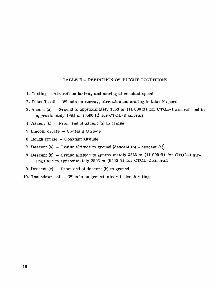
TABLE 11.- DEFINITION OF FLIGHT CONDITIONS

1. Taxiing - Aircraft on taxiway and moving at constant speed

2. Takeoff roll - Wheels on runway, aircraft accelerating to takeoff speed

3. Ascent (a) - Ground to approximately 3353 m (11 000 ft) for CTOL-1 aircraft and to approximately 1981 m (6500 ft) for CTOL-2 aircraft

4. Ascent (b) - From end of ascent (a) to cruise

5, Smooth cruise - Constant altitude

6. Rough cruise - Constant altitude

7. Descent (a) - Cruise altitude to ground (descent (b) + descent (c))

8. Descent (b) - Cruise altitude to approximately 3353 m (11 000 ft) for CTOL-1 aircraft and to approximately 2896 m (9500 ft) for CTOL-2 aircraft

9. Descent (c) - From end of descent (b) to ground

10. Touchdown roll - Wheels on ground, aircraft decelerating

18

TABLE III.- DURATION OF EACH FLIGHT CONDITION FOR EACH FLIGHT

["Percent of time" denotes the ratio of the time for each flight condition to the total time of the flight]

Aircraft Taxiing

of time min of time min of time min of time min of time min oI time min oi time min of time min of time min of time m h Percent Time, Percent Time, Percent Time, Percent Time, Percent Time, Percent Time, Percent Time, Percent Time, Percent Time, Percent Time, flight

Touchdown roll Descent (c) Descent (b) Descent (a) Rough cruise Smooth cruise Ascent (b) Ascent (a) Takeoff roll

CTOL- 1

1 7

.7 .4 30.5 16.5 9.3 5 39.7 21.5 5.6 3 13.5 7.3 17.9 9.7 10.5 5.7 1.3 .7 11.7 6.3 4 1 .8 10.2 7.7. 9.3 7 19.6 14.7 17.3 13 28 21 13.3 10 9 6.8 .9 .7 10.7 8 3 2 .9 25.9 11.9 13 6 38.9 17.9 0 0 16.5 7.6 13 6 10.8 5 1.4 .6 17.4 8 2 0.4 0.8 6.1 11.3 8.2 15.1 14.4 26.4 1.9 3.5 67.4 124 8.7 16 3.3 6 0.4 0.7 3.8

5 .6 .9 5.3 7.9 4.4 6.7 9.7 14.6 5.3 8 52 78 10 15 4.7 7.1 .5 .7 8 iz

5.5 4.8 4.6 7.3

10 4.3 6.2 3

~

0.6 .5 .6 .7 .7 .7 .7 .7 -

~

0.5 .5 .5 .6

1 .5 .6 .4 -

- 1.3 2.3 1.4 2.5 2.5 1.7 1.6 2.8 -

- 1 2.2 1.1 2 3.5 1.3 1.4 1.7 -

CTOL-2

14.6 ' 11.5

0 9 0 35.7 56.1 ' 69.5 25 :::: ::.4

66.4 7 87 11.6 ~ 8.9

57.5 I 2 I 1.6 73

10 7.2 93 66.9

8.3 14 52 87.3 13.1 22 2.7 3 54.3 61 14.6 16.4 2.2 3

12.5 i 12 62.5 I 1 1 1 65

- 27.6 16.3 15.3 16.6 21.4 22.8 21.7 35.3

~

16.4

5.7 10.6 2.6 16.1 10.1 14.4

14.4 10.4 10.9 9.5 8.5 12.5 14.3 8.5

- 0.7 1.1 1.5 1.5

.9 1.3

.9

.9 -

- 0.6 1 1.1 1.2 1.2

.9

.8

.6 -

h3 0

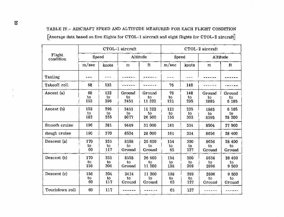
TABLE IV.- AIRCRAFT SPEED AND ALTITUDE MEASURED FOR EACH FLIGHT CONDITION

[Average data based on five flights for CTOL-1 aircraft and eight flights for CTOL-2 aircraft]

CTOL- 1 aircraft CTOL-2 aircraft Flight I condition Speed Altitude Speed Altitude

m/sec ft m knots m/sec ft m h o t s

Taxiing

""" """ 148 76 """ """ 132 68 Takeoff roll

"_ "_ """ """ "_ "- """ """

Ascent (a)

6 185 1885 235 121 11 322 3451 153 298 to to to to to to to to

Ground Ground 148 76 Ground Ground 132 68

r

Ascent (b) 153 298 3451 11 322 121 235 1885 6 185

182 355 80 77 26 500 156 303 8595 28 200

Smooth cruise

28 400 8656 300 154 26 600 8108 33 1 170 Descent (a)

28 400 8656 3 14 161 28 000 8534 3 70 190 Rough cruise

27 900 8 504 314 161 31 000 9449 38 1 196

to to to to

9 500 2896 269 138 11 200 Ground 156 304 to to to to to to to to

28 400 8656 300 154 26 600 8108 331 170 Descent (b)

Ground Ground 127 65 Ground Ground 117 60 to to to to

Descent (c) 156 304 34 14 11 200 138 269 2896 9 500 to to

Ground Ground 127 65 Ground Ground 117 60 to to to to to to

Touchdown roll 60 117 """ """ 65 127 """ """

I

TABLE V.- SUMMARY OF VARIANCE

rBA means "between aircraft" and WA means "within aircraftI3 L

Source of variation

."

BA taxiing WA taxiing

Total

~~

BA takeoff roll WA takeoff roll

- ~~~~

.~ , .. . ~

Total . - - . . . .

BA ascent (a) WA ascent (a)

-~ .. -

Total "- ~. ~

BA ascent (b) WA ascent (b)

. ~ . . . , ~~~~~

Total ~~

_ _ I ~ _ _ c - ~~

BA smooth cruise WA smooth cruise

Total - "~ -.

BA rough cruise WA rough cruise . ~_

Total

BA~descent (a) WA descent (a) ..

Total

BA descent (b) WA descent (b) _ _ _

Total

BA descent (c) WA descent (c)

Total

BA touchdown rol l WA touchdown roll - ~

Total -~

~~~~

Sum of Estimate of Degrees of squares freedom

0.00007500 1 0.00007500

variance

;00008275 10 .00082756

0.00090256 I 11 I 0.00013668

11 .00162739 0.00013668 1 .00014794

~ ~~

0.00176407 I 12

0.0007867 0.0009867 1 ~ ~~~

.00210534

0.000123 1 0.000123

13 0.001230852 .00010257 12 .00123085

0.000000002 1 0.000000002

13 0.00001305 .00000107 12 .00001282

0.00000023 1 0.00000023

0.00103515

.00073465 .00006679 0.0003005 1 ~"F 0.0003005

0.00309204 I 1 7 .00019139 11

~~ ~

~~

- . . ~~

.0016395 .0001491 11

0.0017625

0.00037469

12

0.00037469 1 ,00249272 10 .00024927

0.00286741 11

0.00000009 0.00000009 1 .00207953 10 .00020795

~ ~~ ~ ~. .

0.00207962 0.00016679 0.00016679

11

.00177422 .0001613

0.00194101 12

F- ratio

0.906

0.924

5.16

4.50

0.214

0.00002 1

0.825

1.5

0.00044

1.03

Probabili ty percent

>2 5 .O

>25.0

<5.0

>5 .O

>25.0

>25.0

>25.0

25.0

>25.0

>25.0

21

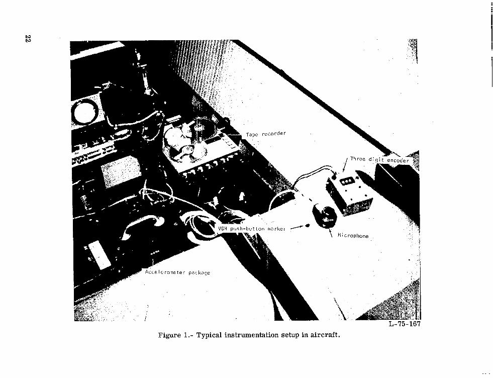
Figure 1.- Typical instrumentation setup in aircraft.

Figure 2.- Photograph of CTOL-1 (three-engine) aircraft.

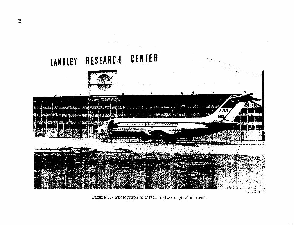
L- 72- 761 Figure 3.- Photograph of CTOL-2 (two-engine) aircraft .

1 Edmonton, AB, Canada

Figure 4.- Flight itineraries of CTOL-1 and CTOL-2 aircraft.

Start 101

takeoff roll

Start 401

Ascent (b) (felt like cruise)

Takeoff roll A (a) CTOL-1 aircraft.

411 Very Tape Tape smooth recorder recorder

I Off On

001 001 101 301

I ascent (b) Start

001 401

”

I

- 1

Speed

. . . . - . . . . . . . . . . . _ . ” . . . .

I I t Ascent (b) Cruise

Takeoff--) roll

(b) CTOL-2 aircraft .

Figure 5.- Sample VGH records. (Numbers refer to code used to identify flight conditions.)

10-

10-

10-

10-

10-

10- ~~ I ~ I I I I I

5 10 15 20 25 30

Frequency, Hz

Figure 6.- Compilation of power spectral density plots measured in the vertical direction at the c.g. during five different descent (a) conditions of the CTOL-2 aircraft.

27

.5

bo

d 0 .rl

Max rime, rnls peak

min g

.1367 4.5 .0267

.1927 3.8 .0233 0.1051 6.0 0.0243

g

.1282 3.8 .0287

.1634 2.4 .0354

.0491 3.2 .0123

7- lo- 0 5 10 15 20 25

Frequency, Hz

100

10

Percent of 1

counts

.1

Cumulative distribution

Percent If time

1 3 5

10 25 50

g level exceeded I

.01 -.6 -.5 -.4 -.3 -.2 -.l 0 .1 .2 .3 .4 .5 .6

Acceleration, g

(a) Taxiing condition.

Figure 7.- Sample power spectral density plot with associated histogram and real-time history of accelerations measured in the vertical direction at the c.g. of the CTOL-1 aircraft .

ta W I

*Plot shown

10- 0 5 10 15 20 25

Frequency, Hz

M s 5 r

10 -

Percent of 1 -


25 .033 50

-.6 -.5 - . 4 - . 3 -.2 -.1 0 .1 .2 -3 .4 .5 .6

Acceleration, g

ded Neg. 0.122 .09 7 .085 .064 .036

0

-

- C 0 .d U

1

Y 4 0)

al 0 1

-.5 I t -4 ' s ec -if ' I ' (b) Takeoff roll.

Figure 7.- Continued.

W 0 Cumulative

distribution

0.0573

.0535

.0568

7.1 .0526

*Plot shown.

-4 \A4 i _

I V r I 0 5 10 15 20 25

Frequency, Hz

loor

0.2461 ,2204

,2073 ,2291

Percent

counts of 1

.1 -

.; 0.144

g level

. 01 -,6 -.5 -.4-.3 -.2 -.1 0 .1 .2 .3 -4 .5 -6

Acceleration, g

- Neg. 0.140

.110

.094 ,065 .032

0

-

-

(c) Ascent (a).


10-2

M .5 r

15.0 *Includes some of ascent (a)

condition. *Plot shown.

I I I I \ J 5 10 15 20 25

Frequency, Hz

I I

lo(

10

Percent

counts of 1

.1

.01


g level

0.086

25 .018 50

I I I I I I I -.6 -.5 -.4 -.3 - .2 -.I 0 .1 .2 .3 .4 .5 .6

Acceleration, g

(d) Ascent (b).


I

Time,

1.2 1.0 1.3

Max r m s I peak I .0059 .0241 .0046 .0133 .0084 .0218 .0060 .0177

6 1 1.2 .0055 .0185 * Plot shown.

0 5 10 15 20 25 -.6 -.5 -.4 -.3 -.2 -.l 0 .I .2 .3 a4 e 5 -6 Frequency, Hz Acceleration, g

(e) Smooth cruise.


2 \ M

cu

Y .3

x" ffl c a, a 4

E

4 Y

a, U

M

10-2, I I 1 4 2.5 I .7

*5 I 5.7 6 I 5.0

*Plot shown.

r m s g

0.0459 .0389 .0399 .0488 .0443 .0336

100 1- I

Percent

counts of 1

.1

0 5 10 1 5 20 25 Frequency, Hz


Percent Df time

1 3 5 10 25 50

g level exceeded I

Acceleration, g

(f) Rough cruise.

Figure 7.- Continued. w w

Run Time, I min

14.7 21.5 14.6

*Plot shown

r m s I .0491 .4632

, .0638 .5342

i -0703 .3903 I 1 .0515 .4514

Frequency, Hz

100

10

Percent

counts of 1

.I

.01 -


Percent

Neg. Pos. Of time exceeded g level

1

0 0 50 .028 .035 25 .074 .071 10 .111 .093 5 .142 .111 3 0.207 0.138

I I I I I I I I I I I I -.5 -.4 -.3 -.2 -.l 0 .I .2 .3 .4 .5 .6

Acceleration, g

-.5 - bo

E 0

.. ...I 42

2-

: 4 a, a, 0

.5

(g) Descent (a).


Time,

5.0

*Plot shown.

rnls g

0.0493 .0271 .0439 .0785 .0368

Max peak

g 0.2561

.1412

.23 54 ,4107

100

10

I I I I \ I 5 10 15 20 25

Frequency, Hz

Percent of 1

counts

.1


g level

10

.01

Acceleration, g

.5 - bD

d

2 .r( U

0

a, w u

- 4

2 -4 sec -

-.5 L I I I I I (h) Descent (b).


100

10

Percent

counts of 1

.1

.01


Percent If time

1 3 5

10 25 50

.I g le1 exce -

Pos. 0.175

.127 ,100 .066

-

.02a 0

re

-.6 -.5-.4-.3 -.2-.1 0 .1 .2 .3 -4 .5 -6 Acceleration, g

1 led Neg. 0.122 -

.oga

.0a3

.063

.03 5 0

(i) Descent ( c ) .


-

-

*Plot shown.

Frequency, Hz

100

10

Percent

counts of 1

.1

.01 “6 -.5-.4 -.3 -.2 -.l 0 .1


g level

11111 .2 .3 .4 .5 .6

Acceleration, g

-3

M

0 d

.rl u 2 a,

(j) Touchdown roll.

Figure 7.- Concluded.

W CD

k (I)

0 B PI

.5 hD

r *4 * PlOl

-03 58 1.9

t shown.

c. 10'70 5 10 15 20 25

Frequency, Hz

100

-1827 10

Percent

counts of 1

.I


Percent )f time

1 3 5 10 25 50

Pos. 0.091 .068 .058 .043 .020 0

. 0 : -.6 -.5 - .4-.3 -.2-.1 0 .I .2 .3 .4

Acceleration, g

led Neg. 0.095

.070

.056

.041

.018 0

- -

-

.5 .6


Figure 8.- Sample power spectral density plot with associated histogram and real-time history of accelerations measured in the vertical direction at the c.g. of the CTOL-2 aircraft .

IO-?,

M .5 r

r / E

Plot shown.

u 5 10 15 20 25

Frequency, Hz

-

r 111s

1.0693 .0712 ,0428 .0426 .0428 .0750 .0524 .0465

rr -

-

- Max peak

0.2792 .3017 .2150 .1750 .2337 .3649 .2819 .le27

(r -

-

loo r

Percent

counts of 1 I

I

Percenl of time

distribution Cumulative

g level exce -

Pos. 0.183 .140 .117 .OB7 .040

0

-

-

Acceleration, g

.084

.039

" L -.5 I I (b) Takeoff roll.


I 100

2 2.27 .0984 .2894 3 2.07 .0906 -2906 4 2.47 .0593 .1417

*5 2.47 .0639 .2180 6 1.73 .0746 .2234 7 1.6 .0966 .4237 Percent

10

8 2.8 I .0635 .1877 counts Of 1

*Plot shown,

10- 7- 5 10 15 20 25

Frequency, Hz

.1

.01 -


g Ievel exceeded

~~-

.076 .078

.040 .033

7 I -.5 -.4-.3 -.2 -.1 0 .1 .2 .3 .4 .5 .6

Acceleration, g

(c) Ascent (a).


'"r Run

* 1 2 3 4 5 6 7 8

-

-

Time, min

14.6 12.5 11.6 15.4 12.6 10.0 16.4 16.4

*Plot shown.

r m s g

0.0301 .0237 .0329 .0448 .0194 .0210 .0150 ,0262

. 5 r

Frequency, Hz

I

Max peak g

0.1891 .1833 .1176 .389 1 .1269 .1336 .0843 .2157

1 lo (

10

Percent

counts of 1

.1

.03 -

Cumulative distribution -

\ -

-

- L

7

-

2 .r

1 1 1 1 1 1 1 1 1 1 1 1 -.5 -.4 -.3-.2 -.l 0 .1 .2 .3 .4 .5 .6

Percent exce

10 .028 25 .013 50 0

Acceleration, g

~

re1 !ded Neg.

0.085 .063 .051 .035 .012 0

(d) Ascent (b).

Figure 8.- Continued

-

Run

1 2 *3 4 5 6 7 8

-

-

Max Time, rms peak

min g g 0.9 0.0061 0.0232 2.2 .0058 .0225 3.5 .0052 .0207 5.3 .0047 .0208 4.0 .0070 .0267 3.8 .0066 .0278 1.5 .0049 .0176 4 .O .0055 .0218

*Plot shown.

Frequency, Hz

loo[


Percent exceeded Of time

g level

'Pos. Neg. 1 0.013 0.011 3 .010 .009 5 .009 .008 10 .007 .006 25 .003 .004 50 0 0

Acceleration, g

(e) Smooth cruise.


k

E 10-6

i \ - f o t s h o - . .

-

Run

1 2 3 4 5 6

+ 7 8

-

-

Time, min 4.2 1.1 1.9 4.5 4.4 2.5 2.3 1.1

. r m s g

0.0257 .0392 .0305 .044 6 .0375 .0401 .0649 .0529

Max peak

g 0.1297 .2667 .1617 .2279 .2077 .2509 .2692 2471 J

100 ,r I

Percent of

counts

’ 5 10 15 20 25

Frequency, Hz Acceleration, g


Percent of time

1 3 5 10 25 50

g level exceeded

Pos. 0.163 .130 -107 .078 -040 0

Neg. 0.168 .132 .lo9 .082 .038

0

(f) Rough cruise.


3un

1 ‘2 3 4 5 6 7 8

- Time,

min 27.6 16.3 15.3 16.4 21.4 22.8 21.7 14.2

r ms g

1.0438 .0544 .0490 .0432 .0359 .079 1 .0417 .0572

peak g

1.3337 .3515 .3119 .2502 .2339 -4130 .2427 .2916

Frequency, Hz

loor

I Percent of

counts

r Cumulative distribution

Percent )f time

1 3 5

10 25 50

g le1 excet ”

Pos. D.180

.127

. lo2

.063 -015 0

ed Veg. D.152 . lo6 .08 6 .054 .018 0

- -

-

.5 - M

d .rl 0

4 sec

- . 3 I I I I I

(g) Descent (a).

Figure 8 . - Continued.

io-2r -

Run

bD *5 r

k 1 2 3 4 5 6 7 8

-

"

- "lot shown I

Time, rms p .0361

11.3 .ON5 .0557

12.2 .0410 .03 60

Frequency, Hz

Max peak

g 0.2731

.1127

.3162

.1932

.lo8 5

.3897

.2259

.3807

100

10

Percent

counts of 1

.1


Acceleration, g

Percent If time

1 3 5

10 25 50

T g level exceeded I Pos. I NeR. I

(h) Descent (b).


i

-

Run

k l

2 3 4 5 6 7

-

a -

I

I I I I 1 5 10 15 20 25

Frequency, Hz

Time, m in 5.7 7.1 7.4 3.3

10.1 14.4 9.5 9 .o

*Plot shown.

rms

1.0584 .0779 .OS70 .0635 .0471

U

.oaw

.0426

.0767

Max peak

g 0.3355

.3422

.2250

.2426

.2258

.4085

.244 3

l o o r

1 Percent of

counts


Percenl 3f time

1 3 5

10 25 50

Acceleration, g

(i) Descent (c).


I L *PlC 10-21"

Run

b 1

2 3 4 5 6 7 8

- Time,

min 0.7 1.1 1.5 1.5 0.9 1.3 0.9 0.9

-

- shown.

A

- rnls

g 1.0723 .OS4 .0534 .04 7 1 .0983 .0634 .0670 .0718 -

t Frequency, Hz

- Peak Max

g 0.4039

.4373

.4711

.4354

.6118

.5799

.4940

.5636 -

10 - 1 I

Percent ,

counts 1 !

of 1 -

.01 .lL -.6 - . 5 -.4 -.:

cu I disl

Percent )f time

1 3 5

10 25 50

nulative tribution

g level exceeded I Pos. 0.198 .141 .118 .088 .04 0 0

- Neg. 0.173 -132 -110 .091 .050

0

-

-

A -.2 -.I 0 .1 .2 .3 .4 .5 .6

Acceleration, g

(j) Touchdown roll.

Figure 8.- Concluded.

.12

.09

.08

.06k

Position

CTOL-2

Flight condition

Figure 9.- Range of vertical rms acceleration values obtained in each flight condition of the CTOL-1 and CTOL-2 aircraft, measured at forward and c.g. positions.

Position

CTOL-2

l o I i

I 1 I I I I I I I Taxiing Takeoff Ascent Ascent Smooth Rough Descent Descent Descent Touchdown

roll (a) (b ) cruise cruise (a) (b) ( 4 roll

Flight condition

Figure 10.- Range of maximum vertical peak accelerations obtained in each flight condition of the CTOL-1 and CTOL-2 aircraft, measured at forward and c.g. positions.

M ..

k 0 +I

a, M

d .d 0

4 cd 0 .d U k

*lo\ .080

"i .040

. 0 2 0 t 0

0 I

0

0 0

1 I Position

1 Aircraft 1 Forward 1 c.g.1

0

0

p" m e

0 e

8 0

e

a'

OJ I I I I I I I I I Taxiing Takeoff Ascent Ascent Smooth Rough Descent Descent Descent Touchdown

roll (a> (b) Cruise Cruise (a) (b) (c) roll

Flight condition

Figure 11.- Means of rms accelerations measured at forward and c.g. positions of the CTOL-1 and CTOL-2 aircraft during different conditions of flight.

0 Taxiing 0 Takeoff

A Ascent b b Rough cruise

0

0

0 0

o@l 0

Q

3 1 0

b Smooth cruise 0 Descent a) 0 Descent 11 0 Descent c 0 Touchdown roll

0 On ground

n t U

u

4 cd .01-

Airborne

0 .01 .02 .03 .04 .05 .06 .07 .08 .09 .10

U

.01-

Airborne

0 .01 .02 .03 .04 .05 .06 .07 .08 .09 .10

Vertical rms acceleration, g

Figure 12.- Rms acceleration values measured in the vertical and lateral directions for each run obtained on the CTOL-2 aircraft at the c.g. position.

I 1 CTOL-1 aircraft v m CTOL-2 aircraft - Mean Value

0 0 d

x

100

80

E?

0 U

0 40t

-%

Y c Q, 0

Taxiing Takeoff Ascent Ascent Smooth Rough Descent Descent Descent Touchdown roll (a> (b ) cruise Cruise (a) (b ) (c) roll

L

Flight condition

Figure 13.- Percentage of vibratory energy within 0- to 3.0-Hz frequency range for both airborne and on-ground flight conditions of the CTOL-1 and CTOL-2 aircraft.

Vertical """ Lateral

5 10 15 20 25

I

1 ' 0 5 10 15 20 25

Frequency Hz

0 5 10 15 20 25

(a) Taxiing condition. (b) Takeoff roll. (c) Touchdown roll.

Figure 14.- Sample PSD plots correspondingly measured in vertical and lateral directions during taxiing, takeoff, and touchdown flight conditions of the CTOL-2 aircraft at.the c.g. position.

-.2 --l*


-.21 I I I l l 1 I 1

(b) Takeoff roll .

-.l -1 - .2 e

l I I l l I I 1 .01 1 10 30 50 70 90 99 99.99

Percent probability

(c) Descent (a).

Figure 15.- Percent probability of exceedance of vertical accelerations measured during taxiing, takeoff, and descent (a) flight conditions on the CTOL-1 aircraft at the c.g. position.

54 NASA-Langley, 1975 L-9531

Documents

VIBRATIONS MEASURED - NASA · PDF fileVIBRATIONS MEASURED IN THE PASSENGER CABINS OF TWO JET TRANSPORT AIRCRAFT 5. Report Date August 1975 6. Performing Organization Code 7. Authorls