Vibration Problem of a Spherical Tank Containing Jet Propellant: Numerical Simulations · 2019-03-13 · 1 Ship Science Report No. 141 ISSN0140-3818 Vibration Problem of a Spherical

1

Ship Science Report No. 141 ISSN0140-3818 Vibration Problem of a Spherical Tank

Containing Jet Propellant: Numerical Simulations

By J. T. Xing, Y. P. Xiong, M. Tan

School of Engineering Sciences, Ship Science, University of Southampton, Southampton SO171BJ

England

&

Makoto Toyota

Structure & Strength Dept., Research Laboratory, IHI, Japan

December 6, 2006

2

CONTENTS

Abstract 4 Chapter 1 Introduction 5 1-1 Background 5

1-2 Objectives 5

1-3 Description of the Tank 7

Chapter 2 Theoretical Modeling and Numerical Method 13 2-1 Governing Equations of the Fluid-Structure Interaction System 13

2-2 Variational formulation and FE Substructure-Subdomain Method 15

2-3 Brief introduction on software- FSIAP 17

Chapter 3 Numerical Results: Natural Frequencies and Modes 19 3-1 General description 19

3-2 Empty Tank 20

3-3 50% water filled with no free surface wave 25

3-4 50% water filled with free surface wave 29

3-5 66% water filled 31

3-6 Fully filled tank 35

3-7 The effect of filled water on the natural frequencies 39

3

3-8 Discussion on the comparison with experimental results 40

Chapter 4 Numerical Results: Dynamic Responses 42 4-1 General description 42

4-2 Empty Tank 42

4-3 50% water filled with no free surface wave 45

4-4 50% water filled with free surface wave 48

4-5 66% water filled 51

4-6 Fully filled tank 54

4-7 Discussion and explanation 57

Conclusions 58

Appendices 59 Data files and explanations 59

References 59

4

Abstract This document is the final report on the joint research project on vibration problem of a spherical tank containing jet propellant between IHI, Japan and SES, University of Southampton, UK. The background of the project is described. The fundamental principles and numerical method used in numerical simulations are presented. The detailed FEA models for each studied cases are given. The calculation results are presented using tables, curves, figures as well as the attached data files. The available experiment results are listed to compare with the numerical calculations. The calculation results show a fundamental agreement with the experiment results. The numerical analysis confirms that:

1) Due to water – tank interaction, the natural frequencies of the water – tank system are decreased with the water level increase. For the 25% water level, the natural frequencies, especially heave mode frequency, shows a significant decrease compared with the empty case. However, with continuing increase the filed water more than 25% level, the decrease gradient of the natural frequencies gradually tends to zero. In the 100% water case, the natural frequency of heave mode is about 200 Hz which can not equal zero.

2) Considering free surface wave effect produces a lot of sloshing modes of very low frequencies compared with the natural frequencies of the dry tank structure. Therefore, for dynamic response analysis with high frequency excitations, the free surface wave may be neglected. However, to assess loads caused by sloshing modes, the free surface waves have to be considered.

3) There exist relative big deformations at the four tank support places in several vibration modes, which may produce a large local stress at support places to cause the product fail in vibration environment. A strengthen local design at the support places is needed.

4) The dynamic response results are affected by damping coefficients of all modes used in the dynamic response analysis. The damping coefficients are approximately presented and therefore, the numerical results are good reference for practical designs.

The report confirms that the original purpose of this joint research project has well completed by IHI and SES.

5

Chapter 1 Introduction 1-1 Background

IHI Japan intends to test and analysis the dynamic behaviors of a spherical tank - water interaction system to solve an industry problem. Professor J T Xing and his colleague in the School of Engineering Sciences (SES) at the University of Southampton (UoS) has produced publications involving theoretical analysis and numerical simulations and has developed software on linear fluid-structure interaction problems in engineering. This background establishes the basis of this joint research between IHI and SES of UoS.

1-2 Objectives The current joint project research intends to investigate the dynamic behavior of a spherical shell-water interaction system using the experiment and numerical simulations based on linear theory of fluid-structure interaction. The Project constitutes a part of the following entire study. 1) Experiment

Exciter test of a spherical tank model is performed to measure its natural frequencies and dynamic responses by IHI.

2) Numerical Simulation of the experimental tank to obtain its natural frequencies and dynamic responses listed as follows using the computer program developed by SES. The planned calculation cases are:

a) Empty tank : Natural frequencies and modes,

One Dynamic response of the tank subjected to a vertical sinusoidal exciter table motion of the frequency (hereinafter referred to as “frequency”) near to the 1-st natural frequency of empty structure.

b) 1/2 water with no free surface (Eigenvalue, one Dynamic response of frequency near

to the fundamental frequency of this whole fluid-structure interaction system). c) 1/2 water with free surface (Eigenvalue, one Dynamic response of frequency near to

the 1st sloshing frequency of this whole fluid-structure interaction system). d) 2/3 water with no free surface (Eigenvalue, one Dynamic response of frequency near

to the fundamental frequency of this whole fluid-structure interaction system

6

e) Fully filled (Eigenvalue, one Dynamic response of frequency near to the fundamental frequency of this whole fluid-structure interaction system)

3) Validation of the calculation results

a) To clarify the phenomenon observed by IHI calculation using its software. That is, with the water volume increasing, the frequency of the water-spherical tank interaction was too low to be physically understood.

b) To compare the calculation frequencies with the experimental results from

engineering point.

Dynamic responses are affected by damping, which relies on experiment by IHI and has important

effects on the results, especially near to the resonance frequency. Therefore, the responses

calculated are a reference for application.

Notes: During the calculation period, the representative of IHI, Mr Makoto Toyoda

visited SES, UoS for three months to discuss and modify the previous working plans to

provide more practical useful results. After the discussions, it has made the following

modifications:

i) Due to the water-shell interactions, the order of vibration modes are changed for

different cases, therefore the motion form of the first natural frequency of each case may

be different. We determine to choose the frequency of the Heavy mode of shell

structure to conduct the dynamic response calculations of the system with no free

surface wave consideration.

ii) The first 5 natural frequencies and the corresponding modes are required to be provided

in the report.

iii) For the dynamic response analysis of each case, the dynamic response curves at different

points are similar so that it is not necessary to draw all response curves at all mea rued

points. We determine only to draw the response curves in the vertical direction at the

top and bottom points on the shell as well as the pressure curves at the pressure measure

points in the report. The all response data for all planed points is provided in the files.

7

1-3 Description of the Tank

A short description on the tank and exciter system provided by IHI is re-presented herein to make a

full document of the report. Fig. 1.1 shows the picture of the model tank. Fig. 1.2 gives the exciter

system used in the test. Fig. 1.3 presents a global view of the tank mounted on the vibration table.

Fig. 1.4 shows the support part of the tank on the vibration table. The geometrical and physical

constants of the tank and water are as follows.

Geometrical and physical constants of the tank Inner diameter 294.4 mm = 29.44cm

Thickness 2.8mm=0.28cm

Young’s modulus 3100MPa = 24 kg/cm1016.3 ×

Poisson’s ratio 0.31

Specific gravity 333 kg/cm1019.1kg/m1190 −×=

Physical constants of water

Specific gravity 333 kg/cm100.1kg/m1000 −×=

Speed of sound m/s1430

Fig. 1.1 Model tank

8

Fig. 1.2 Exciter system

Fig. 1.3 A global view of the tank mounted on the vibration table.

Interface A

9

1. 2. Flange 3. Rib 4. Cylinder 5. Base 6. Cover Plate 7. Spacer Block 8. Support Plate

Fig 1.4. Overall view of tank-support structure: Parts 1-4 are welded construction; Parts 5-7 are used to bolt the tank to the support 1-7 are all made of steel Interface B is connected to interface A in Picture 1-2

Interface B

10

Positions of sensor points and corresponding node numbers in simulations

Fig. 1.5 shows the positions of measurement points in the test. The corresponding node numbers for

each case are listed in Table 1.1-1.5.

Fig. 1.5 The positions of measurement points in the experiment.

11

Tables of the node numbers of accelerometer / pressure sensor locations in numerical meshes There is no node located at the position of pressure sensor 16. Therefore, two points 16a and 16b marked by * are used to give the dynamic response data. Table 1.1 Empty tank

Sensor number

x y z Node numberIn FEA

9 0.0000 0.0000 14.8600 836 5 -7.4300 7.4300 10.5076 671

6,10 7.4300 7.4300 10.5076 681 7,11 7.4300 -7.4300 10.5076 652

8 -7.4300 -7.4300 10.5076 642 12 7.4300 7.4300 -10.5076 321 13 7.4300 -7.4300 -10.5076 292 14 0.0000 0.0000 -14.8600 61

Table 1.2 50% water (with and without free surface wave)

Node numbers for 50% water Sensor Numbers

x y z Tank Sub1 WaterSub2 Global

9 0.0000 0.0000 14.8600 836 1646 5 -7.4300 7.4300 +10.5076 671 1481

6,10 7.4300 7.4300 +10.5076 681 1491 7,11 7.4300 -7.4300 +10.5076 652 1462

8 -7.4300 -7.4300 +10.5076 642 1452 12 7.4300 7.4300 -10.5076 321 1131 1131 13 7.4300 -7.4300 -10.5076 292 1102 1102 14 0.0000 0.0000 -14.8600 61 871 871

16a* 4.7704 -4.7704 -13.2400 212 1022 1022 16b* 6.1762 -6.1762 -12.0220 252 1062 1062

Table 1.3 66.7% water

Node numbers for 66.7% water Sensor Numbers


9 0.0000 0.0000 14.8600 876 5 -7.4300 7.4300 +10.5076 711

6,10 7.4300 7.4300 +10.5076 721 7,11 7.4300 -7.4300 +10.5076 692

8 -7.4300 -7.4300 +10.5076 682 12 7.4300 7.4300 -10.5076 321 1293 1293 13 7.4300 -7.4300 -10.5076 292 1264 1264 14 0.0000 0.0000 -14.8600 61 1033 1033

16a* 4.7704 -4.7704 -13.2400 212 1184 1184 16b* 6.1762 -6.1762 -12.0220 252 1224 1224

12

Table 1.4 100% water

Node numbers for 100% Water Sensor Numbers


9 0.0000 0.0000 14.8600 836 2294 2294 5 -7.4300 7.4300 +10.5076 671 2129 2129

6,10 7.4300 7.4300 +10.5076 681 2139 2139 7,11 7.4300 -7.4300 +10.5076 652 2110 2110 8,15 -7.4300 -7.4300 +10.5076 642 2100 2100 12 7.4300 7.4300 -10.5076 321 1779 1779 13 7.4300 -7.4300 -10.5076 292 1750 1750 14 0.0000 0.0000 -14.8600 61 1519 1519

16a* 4.7704 -4.7704 -13.2400 212 1670 1670 16b* 6.1762 -6.1762 -12.0220 252 1710 1710

13

Chapter 2 Theoretical Modeling and Numerical Method In this chapter, a brief description on the general fluid-structure interaction theory and numerical

method with the software used in this project is presented. The detailed mathematics and practical

examples can be read in the publication papers (Xing and Price 1991, Xing , Price and Du 1996,

Xing, Price and Wang 1997).

2-1 Governing Equations of the Fluid-Structure Interaction System Fig. 2.1 shows a generalized fluid-structure interaction system consisting of a flexible structure of mass density ρ s within a domain sΩ of boundary S ST w∪ ∪ Σ with its unit normal vector ν i and a fluid in a domain fΩ of boundary Σ∪Γ∪Γ∪Γ wpf with a unit normal vectorη i .

Fig.2.1 Schematic illustration of a general fluid - structure interaction system The system is excited by external dynamical forces $ , $ , $T f pi i and ground acceleration $wi . The Cartesian tensor notations (Fung 1977) with subscripts i, j, k and l (=1,2,3) obeying the summation convention are used in the paper. For example, u v w ei i i ij, , , , σ ij and Eijkl represent displacement, velocity, acceleration vector, strain, stress and elastic tensor in the solid, respectively, p denotes the pressure in the fluid. The governing equations describing the dynamics of the coupled fluid - structure interaction problems are as follows. Solid Domain Dynamic equation

isijij wf ρσ =+ ˆ, , ).,(),( 21 tttx si ×Ω∈ (1)

Strain-displacement

14

)(21

,, ijjiij uue += , ).,(),( 21 tttx si ×Ω∈ (2)

Constitutive equation

,klijklij eE=σ ).,(),( 21 tttx si ×Ω∈ (3) and, assuming linearity, we have

)(21,, ,,,,,, ijjitijjitiitii vvedvwuv +==== . (4)

Boundary conditions

acceleration: ,ˆ ii ww = ],,[),( 21 ttStx wi ×∈ (5-1)

traction: ,ijij T=νσ ],,[),( 21 ttStx Ti ×∈ (5-2)

Fluid Subdomain There are two parts for the fluid domain. One is water and another is air. Here, superscript β is used to distinguish fluid domain number. For illustration purpose, it is assumed that two fluid domains are used and therefore 2,1=β in this report. Dynamic equation

)(,

)(2)(, )( βββ

iitt pcp = , ).,(),( 21)( tttx fi ×Ω∈ β (6)

Boundary conditions free surface:

,/)(,

)()(, gpp ttii

βββ η −= ],,[),( 21)( tttx fi ×Γ∈ β (7)

pressure:

,ˆ )()( ββ pp = ],,[),( 21)( tttx pi ×Γ∈ β (8)

acceleration:

,ˆ )()()()()(,

βββββ ηρη iifii wp −= ],[),( 21)( tttx wi ×Γ∈ β . (9)

Interaction interfaces liquid interface between two fluid domains 2,1=β :

15

,011 )2()2(,)2(

)1()1(,)1( =+ ii

fii

f

pp ηρ

ηρ

(10-1)

,)2()1( pp = ],,[),( 21

)12( tttxi ×Γ∈ (10-2) where the gravitational potential of the air on the interface is neglected. Fluid-Structure Interaction Interface:

,/ )()()(,

βββ ρην fiiii pw = ],,[),( 21)( tttxi ×∑∈ β (11-1)

,)()( ββ ηνσ ijij p= ],[),( 21

)( tttxi ×∑∈ β . (11-2)

2-2 Variational Formulations and FE Substructure-Subdomain Method The variational principle (Xing & Price 1991, 1996) is extended to its substructure – subdomain form as follows:

],,[][][],[ ifisisf wpHpHwHwpH ββ Σ++= (12-1)

∫∫ ∫ −Ω−−=Ω )(

2

1)(

ˆ)ˆ21

21(][

IT

Is S iisii

t

t klijijkliisis dtdSwTdwfddEwwwH ρ , (12-2)

,],[ 2

1)(

)()()()( dtdwpwpHt

t iii ∑∫ ∫ΣΣ Γ−=β

βββββ β

η (12-3)

∫

∫∑∫ ∫

Γ

ΓΩ

Γ−

Γ+Ω−=

)(

)(

2

1)(

ˆ

2][

21][

)()()()(

)()(

)(,

)(,)(

)(

)(,

)(,

)(2)(

)(,

)(,

β

ββ

ββββ

ββ

βββ

β

ββ

βββ

ββ

β

η

ρρρ

w

ff

dtdwp

dg

ppd

pp

c

pppH

ii

f

ttf

f

iit

tf

ttf

. (12-4)

This functional is subject to the constraints given in Eqs 2, 4, 5-1, 8 and 10-2 as well as the imposed variation constraints )(0 βδδ pvi == at the two time terminals t1and t2 . The stationary conditions of the functional given in Eq.12 are described in Eqs 1, 5-2, 6, 7, 9, 10-1, 11. A discretization of the solid and fluid media into finite elements expresses the displacement of the solid and the pressure of the fluid using FEA interpolations (Bathe, 1996; Zienkiewicz & Taylor 1989, 1991) in the forms

16

ΨUu =

=

3

2

1

uuu

, (13-1)

)()( ββ Θp=p , (13-2)

where Ψ and )(βΘ denote the interpolation function matrices and U and p ( )β represent the global node displacement / pressure vector, respectively. The functional Hsf given in Eq. 12 now takes the form

,)ˆ21

21(

)()ˆ21

21(],[

2

1

)(

)(2

1

2

1

∫∑

∫∑∫

−−+

−−−=

t

t

TTT

t

t

TTTt

t

Tsf

dt

dtdtH

β

β

β

β

uppkppmp

URpFUUKUUMUUp

&&&&

&&&&&&&&&&&&

(14)

where M and K represent respectively the finite-element mass and stiffness matrices of the dry structure; m ( )β and k ( )β represent the finite-element matrices of the fluid domain, R ( )β denotes the fluid-structure interaction matrix. The stationary conditions of the functional in Eq.14 is the finite equation of the air - liquid - structure dynamic interaction system

.)2(

)1(

)2(

)1(

(2)

(1)

(2)T(1)T

)2(

)1(

(2)(2)

(1)(1)

=

−−+

ffF

ppU

k000k0

RRK

ppU

m0R0mR00M

&&

&&

&&

(15)

Introduce the following matrices

,,, )2(

)1(

)2(

)1(

)2(

)1(

=

=

=ff

fpp

pRR

R

(16)

,, )2(

)1(

)2(

)1(

=

=

k00k

km0

0mm

then Eq.15 becomes

,

=

−+

fF

pU

k0RK

pU

mR0M T

&&

&& (17)

which can be transformed into the symmetric form (Xing & Price, 1991) as

17

,11

11

=

+−−

+

−−

−−

fF

pU

RMRkKRMRMKKMK

pU

m00M

TT

TTT

&&

&& (18)

This equation can be solved by using a mode superposition method or a time integral method as usually adopted in a general finite element analysis. For natural vibrations of the system, the force vector on the right hand side of Eq.18 vanishes. 2-3 Brief introductions on software FSIAP

To complement the mixed finite element substructure-subdomain method presented herein, a specialized Fluid – Structure Interaction Analysis Program-FSIAP (Xing 1995a, b) based on PC computer architecture was further developed to solve natural vibration and dynamical response problems associated with structure, fluids and their interactions. This user-friendly software contains all the theoretical features discussed in the development of the approach and overcomes restrictions on computer storage capacity, length of run time etc, providing an efficient solution to complex fluid-structure dynamical interaction problems. The main flow chart of FSIAP is shown in Fig.2.2 Here, this program is used to calculate the natural characteristics and dynamic responses excited by base motion of the water tank interaction system. The engineering unit system is used in the program. That is Length cm Force kg Time s The output data can give the natural frequencies and the corresponding natural modes as well as the dynamic responses of the system excited forces applied or the ground motion. The dynamic response output data is given in the following format. * Node number * - (Component number) defined as: Node number: node number in the substructure or subdomain mesh, Component number = 1 x- direction displacement = 2 y- direction displacement = 3 z- direction displacement = 4 rotation about x- direction = 5 rotation about y- direction = 6 rotation about z- direction = 7 fluid pressure in fluid subdomain

18

Fig.2.2 Main flow chart of computer program FSIAP

Start

Input main control data

Sub methods ?

Sub data Global data

N Y

No

Substructure and subdomain FEA Analysis

Re-St

Synthesis

Dynamic code

Sp

Output

Sub+1

Y

Dynamic response

by time integration

Natural vibration

analysis

Dynamic response

by mode summation

19

Chapter 3 Numerical Results: Natural Frequencies and Modes 3-1 General description Coordinate system

As shown in Fig. 3.1, a Cartesian system O-xyz of origin at the centre of the tank is chosen as a

global reference system in numerical analysis. All node positions used in this report are given

under this coordinate system. The support points marked by the black dots in Fig. 3.1 are treated as

fixed boundary to calculate the natural vibration characteristics.

Fig. 3.1. The global coordinate system and the mesh structure of the solid tank

Finite element meshes

For the tank structure, 4 node plate – shell element is used as shown in Fig. 3.1 For the water

domain, 8-node fluid pressure elements are used. Fig. 3.2 shows the mesh structure for the 50%

water domain, where Fig. 3.2a) gives a view from a side direction of the ball and b) provides a view

from the top of the tank.

20

Fig. 3.2 The mesh structure of the water domain: a) a view from a side direction of the tank;

b) a view from the top of the tanks

In this simulation, the solid tank is considered as a substructure and the water is treated as a

fluid domain. The detailed element number, node number and the degree number of freedom used

in the calculations are presented in the following sub-sections. More detailed data can be found in

the data files given in the report.

Natural frequencies and modes

For each case, as mentioned in Chapter 1, the first 5 natural frequencies and the corresponding

natural modes are listed in the following sub-sections of this chapter. The input files and output

files for all cases are given in this report, from which more detailed data on the natural frequencies

and modes can be read.

3-2 Empty Tank FEA model

Number of nodal points 841

Number of plate-shell elements 820

Number of degree of freedom 4812

Number of natural frequencies and modes calculated 12

21

Natural frequencies (Hz) mode = 1, freq. = 774.81000 mode = 2, freq. = 774.81000 mode = 3, freq. = 867.46997 mode = 4, freq. = 867.46997 mode = 5, freq. = 1143.40002 Natural modes: The first five natural modes are shown in Fig. 3.3 a)-e). The first mode and the second mode have same frequency 774.8Hz and show two sway motion forms along two horizontal directions. The third and fourth modes behave two roll motion forms about two horizontal directions. The fifth mode behaves a heave motion along the vertical direction. a) Mode 1 (774.8Hz): a sway vibration form in x-direction

b) Mode 2 (774.8Hz): a sway vibration form in y-direction

22

Fig. 3.3 The first natural modes of the empty tank

c) Mode 3 (867.5Hz): a roll vibration form about x-direction

d) Mode 4 (867.5Hz): a roll vibration form about y-direction

e) Mode 5 (1143.4Hz): a heave vibration form in z-direction

23

Experimental results Fig 3.4 shows 5 curves obtained from the experiment. From these curves, we find the following peak frequencies: 633Hz, 656Hz, 674Hz, 773Hz, 768Hz, 814Hz and 832Hz. There is no experimental mode form data available to identify the mode for comparison with the calculations. However, the first natural frequency 774.8Hz calculated may be corresponds to 773Hz of experimental result.

0

2

4

6

8

10

12

14

16

18

20

0 200 400 600 800 1000

Frequency(Hz)

Transfer Function(Acc.

CH-9(V)[Mag]

CH-14(V)[Mag]

0

2

4

6

8

10

12

14

16

0 200 400 600 800 1000

Frequency(Hz)


CH-5(V)[Mag]

CH-6(V)[Mag]

CH-7(V)[Mag]

CH-8(V)[Mag]

24

Fig. 3.4 Five curves obtained in the experiment

0

0.5

1

1.5

2

2.5

3

3.5

4

0 200 400 600 800 1000

Frequency(Hz)

Power Spectru

CH-5(V)

CH-6(V)

CH-7(V)

CH-8(V)

0

0.5

1

1.5

2

2.5

3

3.5

4

0 200 400 600 800 1000

Frequency(Hz)

Power Spectru

CH-9(V)

CH-10(V)

CH-11(V)

CH-12(V)

0

0.5

1

1.5

2

2.5

3

3.5

4

0 200 400 600 800 1000

Frequency(Hz)

Power Spectru

CH-13(V)

CH-14(V)

25

3-2 50% water filled tank with no free surface wave included FEA model



Number of fluid elements 1000

Number of degree of freedom for solid 4813

Number of degree of freedom for fluid 1210


Natural frequencies (Hz) mode = 1, freq. = 260.98999 mode = 2, freq. = 274.01999 mode = 3, freq. = 274.13000 mode = 4, freq. = 404.20999 mode = 5, freq. = 505.79999 Natural modes: The first five natural modes are shown in Fig. 3.5 a)-e). As shown in this figure, due to water-tank interactions, there are obvious changes of vibration modes. The first mode is now the heave motion mode with frequency 260.99Hz. The second and third modes have same frequency 274.02Hz and show two sway motion forms along two horizontal directions. Compared with the empty case, the motion of the tank bottom filled by water is larger than the top tank where no water filled. The fourth mode shows a compression and expansion motion form in two horizontal directions, respectively, and the tank bottom motion is bigger. The fifth mode behaves a more complex deformation. a) Mode 1 (260.99Hz)

26

b) Mode 2 (274.02Hz) c) Mode 3 (274.13Hz)

27

d) Mode 4 (404.21Hz) e) Mode 5 (505.80Hz)

Fig. 3.5 The first five natural vibration modes obtained in simulations

Experiment Results Fig. 3.6 presents three experimental curves measured at sensor 6 and 7. From these figures, there the following frequencies observe red: 270Hz, 311Hz, 533Hz, 656Hz and 662Hz. Here the frequency 270Hz is well agreed with the first calculation frequency of heave mode.

28

Fig. 3.6 Three experimental curves for 50% water tank with no free

surface wave considered.

0

1

2

3

4

5

6

7

8

9

0 200 400 600 800 1000

Frequency(Hz)


CH-5(V)[Mag]

CH-6(V)[Mag]

CH-7(V)[Mag]

CH-8(V)[Mag]

0

2

4

6

8

10

12

14

0 200 400 600 800 1000

Frequency(Hz)


CH-12(V)[Mag]

CH-13(V)[Mag]

0

5

10

15

20

25

30

0 200 400 600 800 1000

Frequency(Hz)


CH-9(V)[Mag]

CH-14(V)[Mag]

29

3-4 50% water filled tank with free surface wave considered FEA model







Natural frequencies (Hz) mode = 1, freq. = 0.00000 mode = 2, freq. = 1.62480 mode = 3, freq. = 1.62480 mode = 4, freq. = 2.20130 mode = 5, freq. = 2.20640 Natural modes: The first five natural modes are shown in Fig. 3.7 a)-e). Due to the free surface wave is considered, the natural frequencies of the system are much lower than the case of neglecting free surface wave. The main modes of the system are sloshing modes. As shown in this figure. The first mode is a static mode with zero frequency which is similar to the rigid mode of structure vibration. The second and third modes have same frequency 1.6248Hz and show two sloshing motions. The fourth and fifth modes show two similar modes with frequency about 2.2Hz. a) Mode 1 (0Hz) Constant pressure mode

30

b) Mode 2 (1.625Hz)

c) Mode 3 (1.625Hz)

d) Mode 4 (2.20Hz)

31

Experimental results Not available.

3-5 66% water filled tank FEA model







Natural frequencies (Hz) mode = 1, freq. = 246.06000 mode = 2, freq. = 246.06000 mode = 3, freq. = 252.28000 mode = 4, freq. = 381.92999 mode = 5, freq. = 431.64999 Natural modes: The first five natural modes are shown in Fig. 3.8 a)-e). The first and second modes have a same frequency 246.06Hz with the motion forms similar to the 2nd and 3rd modes in the 50% water case. The third mode is the heave motion mode with frequency 252.28Hz. The fourth mode of frequency 381.93Hz and the fifth mode of frequency 431.65Hz are similar to the ones for the case of 50% water filed tank.

e) Mode 5 (2.21Hz)

32

b) Mode 3 (252.28Hz)

a) Mode 1 and b) Mode 2 (246.06Hz)

33

Experiment Results Fig. 3.9 shows three curves obtained in the experiment, from which three frequencies are found: 275Hz, 469Hz and 480Hz.

e) Mode 5 (431.65Hz)

Fig. 3.8 The first five natural modes of 66% water filed tank

d) Mode 4 (381.93Hz)

34

Fig. 3.9 The three curves obtained in the experiment

0

1

2

3

4

5

6

7

8

9

0 100 200 300 400 500

Frequency(Hz)


CH-5(V)[Mag]

CH-6(V)[Mag]

CH-7(V)[Mag]

CH-8(V)[Mag]

0

2

4

6

8

10

12

14

16

0 100 200 300 400 500

Frequency(Hz)


CH-12(V)[Mag]

CH-13(V)[Mag]

0

5

10

15

20

25

0 100 200 300 400 500

Frequency(Hz)


CH-9(V)[Mag]

CH-14(V)[Mag]

0

1

2

3

4

5

6

7

8

9

0 100 200 300 400 500

Frequency(Hz)


CH-10(V)[Mag]

CH-11(V)[Mag]

35

3-6 Fully filled tank FEA model







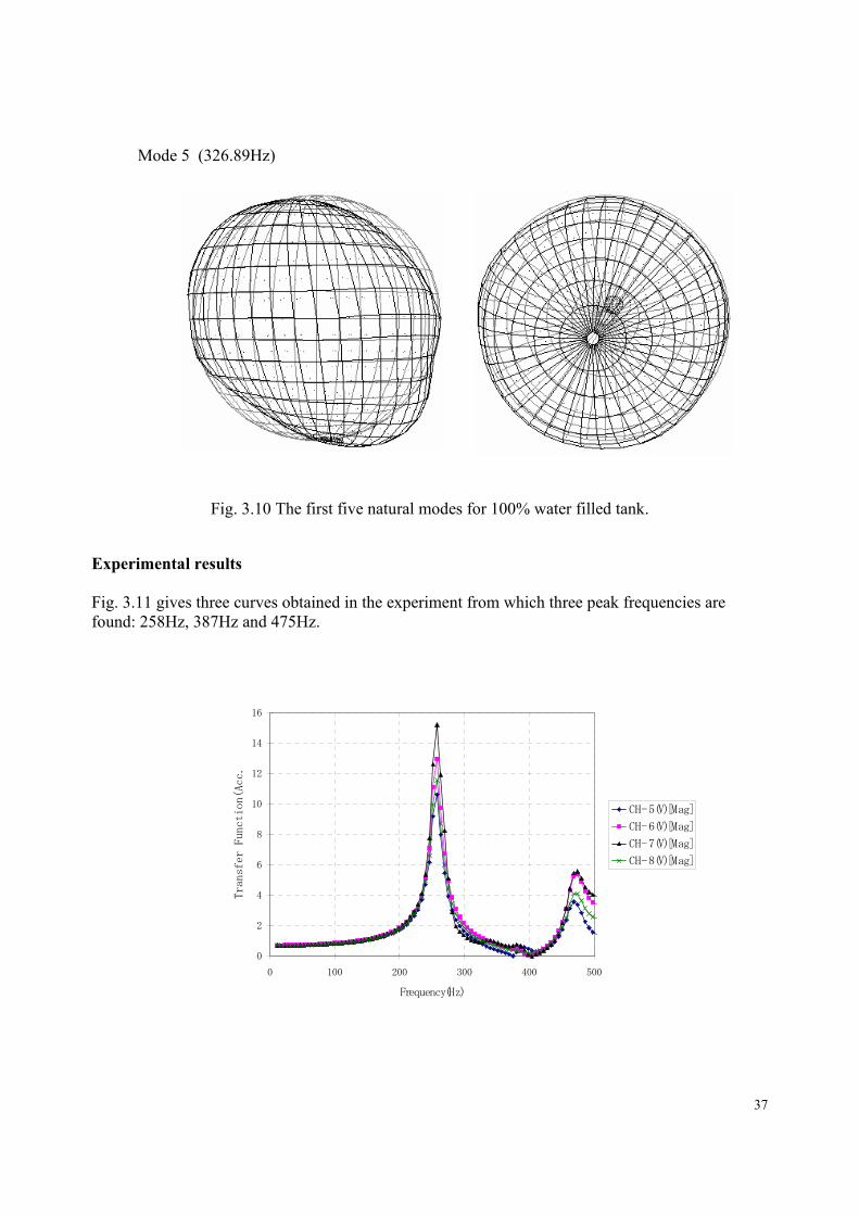
Natural frequencies (Hz) mode = 1, freq. = 196.66000 mode = 2, freq. = 196.66000 mode = 3, freq. = 201.24001 mode = 4, freq. = 322.81000 mode = 5, freq. = 326.89001 Natural modes: The first five natural modes are shown in Fig. 3.10 a)-e). The first and second modes have an approximately same frequency 196.6 Hz with the motion forms similar to the 2nd and 3rd modes in the 50% and 66% water cases. The third mode is the heave motion mode with frequency 201.2Hz. The fourth mode of frequency 322.8Hz and the fifth mode of frequency 326.89Hz are similar to the ones for the cases of 50% and 66% water filed tank.

Mode 1 (196.6Hz)

36

Mode 3 (201.2Hz)

Mode 4 (322.8Hz)

Mode 2 (196.7Hz)

37

Fig. 3.10 The first five natural modes for 100% water filled tank.

Experimental results Fig. 3.11 gives three curves obtained in the experiment from which three peak frequencies are found: 258Hz, 387Hz and 475Hz.

Mode 5 (326.89Hz)

0

2

4

6

8

10

12

14

16

0 100 200 300 400 500

Frequency(Hz)


CH-5(V)[Mag]

CH-6(V)[Mag]

CH-7(V)[Mag]

CH-8(V)[Mag]

38

Fig. 3.11 Three curves obtained in the experiment

0

5

10

15

20

25

0 100 200 300 400 500

Frequency(Hz)


CH-9(V)[Mag]

CH-14(V)[Mag]

0

2

4

6

8

10

12

0 100 200 300 400 500

Frequency(Hz)


CH-10(V)[Mag]

CH-11(V)[Mag]

39

3-7 The effect of filled water level on the natural frequencies

Table 3.1 listed the natural frequencies obtained in the calculations which are arranged according to

the identified mode shapes. Fig. 3.12 gives a curve to show the effect of the water level on the

heave natural frequency. To better to study the water level effect, the first three frequencies of 25%

water level tank, which is not required in the contract, are added.

Table 3.1 The effect of filled water level on the natural frequencies (Hz)

Mode 0% water 25% water 50% water 66.7% water 100% water

Heave 1143.4 335.8 260.99 252.28 201.2

Sway 774.8 502.1 274.13 246.06 196.6

Sway 774.8 502.1 274.13 246.06 196.7

867.5* 404.21 381.95 322.8

867.5* 505.80 431.65 326.89

*Note: These two mode frequencies obtained for the empty tank case are listed here for a reference

only because the mode shapes are different if compared with the cases of filled water.

From Table 3.1 and Fig. 3.12 as well as the results presented in this chapter, we may conclude that:

1) The filled water change the order of vibration mode, such as, the heave mode is the fifth

mode for the empty case but is the first mode for 50% water level case and the third mode for 66%

and 100% water level cases.

2) There is a significant decrease of the natural frequencies due to 25% filled water. However,

after the filled water level higher that 25%, the increase of water level does not significantly

decrease the natural frequencies of similar vibration mode shapes.

3) The decrease gradient of the natural frequency as a function of water level tends to small

constant.

4) It is not possible that there is a zero natural frequency for any water level filled tank with no

free surface wave considered.

5) The free surface wave effect causes a lot of water sloshing modes with very lower

frequencies than the natural frequencies of the dry tank structure.

40

Fig. 3.12 The effect of water level on the natural frequency of the heave vibration mode of water-

tank interaction system

3-8 Discussion on the comparison with experimental results The numerical results and some experimental results have been presented in previous sections of

studied cases to provide a comparison. As mentioned in the related sections, we can say that the

important frequencies obtained in the numerical simulations are basically agreeable with the

experiment results. However, the following factors are needed to be considered to understand the

possible error in both numerical and experimental process.

Boundary condition of tank support

In the numerical model, the tank is ideally fixed at three points of each support part as shown in Fig.

3.1. It was investigated that fixed four rectangle area of the shell surface on where four supports are

connected does not make any obvious change for natural frequencies of the empty tank. In the

experimental device, these four support parts are fixed by bolts, of which the stiffness of support is

affected by the bolt forces. These non-fully determined factors are difficult to be simulated in the

numerical model.

0 20 40 60 80 1000

200

400

600

800

1000

1200

Water level (%)

Freq

uenc

y of

hea

ve m

ode

(Hz)

41

Additional mass and stiffness of sensors

The additional mass and stiffness of sensors are not considered in the numerical model to provide

the numerical results for real product analysis use.

Mode shape identification

To measure the natural frequencies and the corresponding modes, the use of resonance test

equipment is necessary. It is very difficult to measure vibration mode shapes which are affected by

the phase of vibration signals measured using vibration table test. We have not got mode shape

experiment results, and therefore it is difficult to identify the suitable mode to compare the results.

42

Chapter 4 Numerical Results: Dynamic Responses 4-1 General description In the dynamic response analysis, the tank system is excited by a vertical sinusoidal motion of

acceleration amplitude 1g, i.e. 2cm/s981 . The damping coefficients of the modes used in the

calculations are listed in Table 4.1. The output points of displacement or pressure responses and

their correspondence to the sensors position are listed in Table 1.1-1.5. The notations of output

responses in the output data files are given in section 2-3. The mesh and FEA model of numerical

calculation for each case are same as the analysis of natural vibration calculations presented in the

chapter 3.

Table 4.1 Damping coefficients used in the calculations of dynamic responses. The data is provided

from the experiment curves calculated by IHI representative

Case Empty 50% 67% 100% Exp.No No.4 No.7 No.9 No.16 Ch.No No.9 No.14 No.14 No.14

Frequency (Hz) 826 311 275 258 Peak value 17.3 24.3 22.9 20.3

0.707 Peak value 12.2 17.2 16.2 14.4 Half-power band width 65 20 16 16

ζ 0.039 0.032 0.029 0.031

In this report, the displacement or pressure response curves at selected points are plotted for each

case. The maximum response amplitudes are listed in the tables. The more detailed data can be

read in the output data flies including in the report.

4-2 Empty Tank For the empty case, the frequency of heave mode is 1143.4Hz of which the damping confident is

not provided, but the damping 0.039 is still used in dynamic response calculation.

Base motion

Frequency 1143.4Hz

Acceleration amplitude 1g = 2cm/s981

43

Related data in calculation

Retained mode number 145

Maximum frequency of retained modes 2316.4Hz

Damping coefficient 0.039

Time step 0.00005s

Calculation time step 300

Output step interval 2

Table 4.2 shows the maximum amplitudes at interest points and arriving times. Fig. 4.1 shows the

displacement response curves at top sensor point 9 and the bottom sensor point 14.

Table 4.2 Maximum displacement values and arriving time at interest points

Node- (component)

61-(1) 61-(2) 61-(3) 292-(1) 292-(2) 292-(3)

Values (cm) 3.868375D-08 4.186292D-08 2.797310D-04 1.082624D-05 1.083551D-05 1.756679D-04 Time (s) 7.000000D-04 7.000000D-04 1.450000D-02 1.410000D-02 1.410000D-02 1.230000D-02 Node- (component)

321-(1) 321-(2) 321-(3) 642-(1) 642-(2) 642-(3)


652-(1) 652-(2) 652-(3) 671-(1) 671-(2) 671-(3)


681-(1) 681-(2) 681-(3) 836-(1) 836-(2) 836-(3)

Values (cm) 1.138621D-05 1.138791D-05 1.713614D-04 5.589613D-09 3.348093D-06 2.736102D-04 Time (s) 1.410000D-02 1.410000D-02 1.230000D-02 1.800000D-03 1.320000D-02 1.100000D-02

44

Fig. 4.1 The time response histories in z-direction at top sensor 9 and bottom sensor 14 of the tank

0 0.005 0.01 0.015-3

-2

-1

0

1

2

3

4x 10-4

Time (s)

Rel

ativ

e di

spla

cem

ent Z

(cm

)

Empty tank:

Sensor 9, f = 1143.4Hz, damping = 0.039

0 0.005 0.01 0.015-3

-2

-1

0

1

2

3

4x 10-4

Time (s)

Rel

ativ

e di

spla

cem

ent Z

(cm

)

Empty tank:


45

4-3 50% water filled with no free surface wave Base motion

Frequency 260.99Hz






Time step 0.0002s



Table 4.3 shows the maximum amplitudes at interest points and arriving times. Fig 4.4 shows the

pressure response at points 16a) and 16b). Fig. 4.5 shows the displacement response curves at top

sensor point 9 and the bottom sensor point 14.

Table 4.3 Maximum displacement and pressure values and arriving time at interest point

Node- (component) 61-(1) 61-(2) 61-(3) 212-(1) 212-(2) 212-(3)

Values (cm) 5.501976D-05 3.664841D-05 7.195841D-03 9.924487D-05 1.454330D-04 5.668927D-03 Time (s) 5.440000D-02 5.440000D-02 5.200000D-02 4.600000D-02 5.400000D-02 5.200000D-02 Node- (component) 252-(1) 252-(2) 252-(3) 292-(1) 292-(2) 292-(3)



Values (cm) 3.774747D-05 2.342599D-05 8.055954D-04 2.529829D-05 4.091305D-05 8.073486D-04 Time (s) 5.240000D-02 1.200000D-03 5.960000D-02 1.200000D-03 5.240000D-02 5.960000D-02Node- (component) 681-(1) 681-(2) 681-(3) 836-(1) 836-(2) 836-(3)

Values (cm) 2.624061D-05 2.994771D-05 7.824668D-04 1.489080D-05 1.545223D-05 8.043945D-04 Time (s) 5.240000D-02 5.240000D-02 5.960000D-02 5.800000D-02 5.400000D-02 5.200000D-02Node- (component) 871-(7) 1022-(7) 1062-(7) 1102-(7) 1131-(7)

Values (kg/cm2) 2.342820D-01 1.732077D-01 1.361906D-01 9.834280D-02 9.782718D-02 Time (s) 5.200000D-02 5.200000D-02 5.200000D-02 5.960000D-02 5.960000D-02

46

Fig. 4.4 The time response histories at point 16a) and 16b).

0 0.01 0.02 0.03 0.04 0.05 0.06-0.2

-0.15

-0.1

-0.05

0

0.05

0.1

0.15

0.2

Time (s)

Pre

ssur

e P

(kg

/ cm

2)

50% Water (no free surface wave):

Sensor 16a, f = 260.99Hz, damping = 0.032

0 0.01 0.02 0.03 0.04 0.05 0.06-0.2

-0.15

-0.1

-0.05

0

0.05

0.1

0.15

Time (s)

Pre

ssur

e P

(kg

/ cm

2)

50% Water (no free surface wave):

Sensor 16b, f = 260.99Hz, damping = 0.032

47


0 0.01 0.02 0.03 0.04 0.05 0.06-1

-0.8

-0.6

-0.4

-0.2

0

0.2

0.4

0.6

0.8

1x 10-3

Time (s)

Rel

ativ

e di

spla

cem

ent Z

(cm

)

50% Water (no free surface wave):Sensor 9, f = 260.99Hz, damping = 0.032

0 0.01 0.02 0.03 0.04 0.05 0.06-8

-6

-4

-2

0

2

4

6

8x 10-3

Time (s)

Rel

ativ

e di

spla

cem

ent Z

(cm

)

50% Water (no free surface wave):Sensor 14, f = 260.99Hz, damping = 0.032

48

4-4 50% water filled with free surface wave Base motion

Frequency 1.6248Hz






Time step 0.02s





sensor point 9 and the bottom sensor point 14. In this case, due to the constant pressure mode with

zero frequency, the mean values of the response curves do not equal zero, which is caused by zero

frequency motion.

Table 4.4 Maximum displacement and pressure values and arriving time at interest points

Node -(component)

61-(1) 61-(2) 61-(3) 212-(1) 212-(2) 212-(3)

Values (cm) 1.791913D-06 2.448165D-06 3.691236D-04 7.549681D-06 4.763217D-06 3.032478D-04 Time (s) 2.160000D+00 2.160000D+00 9.200000D-01 2.160000D+00 5.840000D+00 9.200000D-01 Node -(component)

252-(1) 252-(2) 252-(3) 292-(1) 292-(2) 292-(3)

Values (cm) 1.481710D-06 3.400669D-06 2.624043D-04 1.569331D-05 1.669615D-05 2.212543D-04 Time (s) 5.840000D+00 9.200000D-01 9.200000D-01 9.200000D-01 9.200000D-01 9.200000D-01 Node -(component)

321-(1) 321-(2) 321-(3) 642-(1) 642-(2) 642-(3)

Values (cm) 1.036716D-05 8.847735D-06 2.373988D-04 1.138359D-05 1.359740D-05 1.469821D-04 Time (s) 9.200000D-01 9.200000D-01 9.200000D-01 4.000000D+00 4.000000D+00 4.000000D+00 Node -(component)

652-(1) 652-(2) 652-(3) 671-(1) 671-(2) 671-(3)

Values (cm) 9.662340D-06 1.321839D-05 1.507026D-04 7.220443D-07 5.032217D-06 1.844108D-04 Time (s) 4.000000D+00 4.000000D+00 4.000000D+00 3.200000D-01 9.200000D-01 4.000000D+00Node -(component)

681-(1) 681-(2) 681-(3) 836-(1) 836-(2) 836-(3)

Values (cm) 4.097802D-06 6.642083D-06 1.911852D-04 9.103065D-08 9.083971D-06 2.406413D-04 Time (s) 2.160000D+00 2.160000D+00 4.000000D+00 1.520000D+00 4.000000D+00 4.000000D+00Node -(component)

871-(7) 1022-(7) 1062-(7) 1102-(7) 1131-(7)

Values (kg/cm2 2.059507D-02 2.059796D-02 2.059990D-02 2.060172D-02 2.060162D-02 Time (s) 4.000000D+00 4.000000D+00 4.000000D+00 4.000000D+00 4.000000D+00

49


0 1 2 3 4 5 60

0.005

0.01

0.015

0.02

0.025

Time (s)

Pre

ssur

e P

(kg

/ cm

2)

50% Water (with free surface wave):

Point 16b, f = 1.6248Hz, damping = 0.032

0 1 2 3 4 5 60

0.005

0.01

0.015

0.02

0.025

Time (s)

Pre

ssur

e P

(kg

/ cm

2)


Point 16a, f = 1.6248Hz, damping = 0.032

50


0 1 2 3 4 5 6-3

-2.5

-2

-1.5

-1

-0.5

0x 10-4

Time (s)

Rel

ativ

e di

spla

cem

ent Z

(cm

)


Sensor 9, f = 1.6248Hz,damping = 0.032

0 1 2 3 4 5 6-4.5

-4

-3.5

-3

-2.5

-2

-1.5

-1

-0.5

0x 10-4

Time (s)

Rel

ativ

e di

spla

cem

ent Z

(cm

)


Sensor 14, f = 1.6248Hz,damping = 0.032

51

4-5 66% water filled Base motion

Frequency 252.28Hz






Time step 0.0001s





sensor point 9 and the bottom sensor point 14.

Table 4.5 Maximum displacement and pressure values and arriving time at interest points Node- (component)

61-(1) 61-(2) 61-(3) 212-(1) 212-(2) 212-(3)


252-(1) 252-(2) 252-(3) 292-(1) 292-(2) 292-(3)


321-(1) 321-(2) 321-(3) 682-(1) 682-(2) 682-(3)


692-(1) 692-(2) 692-(3) 711-(1) 711-(2) 711-(3)


721-(1) 721-(2) 721-(3) 876-(1) 876-(2) 876-(3)


1033-(7) 1184-(7) 1224-(7) 1264-(7) 1293-(7)

Values (kg/cm2 3.409952D-01 2.609487D-01 2.119302D-01 1.610124D-01 1.601019D-01 Time (s) 5.960000D-02 5.960000D-02 5.960000D-02 5.960000D-02 5.960000D-02

52


0 0.01 0.02 0.03 0.04 0.05 0.06-0.4

-0.3

-0.2

-0.1

0

0.1

0.2

0.3

Time (s)

Pre

ssur

e P

(kg

/ cm

2)

66.7% Water:


0 0.01 0.02 0.03 0.04 0.05 0.06-0.25

-0.2

-0.15

-0.1

-0.05

0

0.05

0.1

0.15

0.2

0.25

Time (s)

Pre

ssur

e P

(kg

/ cm

2)

66.7% Water:


53


0 0.01 0.02 0.03 0.04 0.05 0.06-0.015

-0.01

-0.005

0

0.005

0.01

0.015

Time (s)

Rel

ativ

e di

spla

cem

ent Z

(cm

)

66.7% Water:


0 0.01 0.02 0.03 0.04 0.05 0.06-1.5

-1

-0.5

0

0.5

1

1.5x 10-3

Time (s)

Rel

ativ

e di

spla

cem

ent Z

(cm

)

66.7% Water:Sensor 9, f = 252.28Hz, damping = 0.029

54

4-6 Fully filled tank Base motion

Frequency 201.24Hz






Time step 0.0002s




pressure response at points 15, 16a) and 16b). Fig. 4.11 shows the displacement response curves at

top sensor point 9 and the bottom sensor point 14.

Table 4.6 Maximum displacement and pressure values and arriving time at interest points Node -(component)

61-(1) 61-(2) 61-(3) 212-(1) 212-(2) 212-(3)

Values (cm) 6.525720D-05 5.217052D-05 1.249957D-02 2.330684D-04 2.721218D-04 1.038725D-02 Time (s) 5.880000D-02 5.920000D-02 5.480000D-02 5.760000D-02 5.720000D-02 5.480000D-02 Node -(component)

252-(1) 252-(2) 252-(3) 292-(1) 292-(2) 292-(3)


321-(1) 321-(2) 321-(3) 642-(1) 642-(2)

642-(3)

Values (cm) 5.087057D-04 5.026793D-04 7.649083D-03 3.795461D-04 3.644999D-04 5.744757D-03Time (s) 5.720000D-02 5.720000D-02 5.480000D-02 5.720000D-02 5.720000D-02 5.480000D-02Node -(component)

652-(1) 652-(2) 652-(3) 671-(1) 671-(2) 671-(3)


681-(1) 681-(2) 681-(3) 836-(1) 836-(2) 836-(3)


1519-(7) 1670-(7) 1710-(7) 1750-(7) 1779-(7) 2100-(7)

Values(kg/cm2) 8.226359D-01 7.630379D-01 7.257821D-01 6.863414D-01 6.862409D-01 4.613993D-01 Time (s) 5.480000D-02 5.480000D-02 5.480000D-02 5.480000D-02 5.480000D-02 5.480000D-02

55

0 0.01 0.02 0.03 0.04 0.05 0.06-0.5

-0.4

-0.3

-0.2

-0.1

0

0.1

0.2

0.3

0.4

0.5

Time (s)

Pre

ssur

e P

(kg

/ cm

2)

100% Water:


0 0.01 0.02 0.03 0.04 0.05 0.06-0.8

-0.6

-0.4

-0.2

0

0.2

0.4

0.6

0.8

Time (s)

Pre

ssur

e P

(kg

/ cm

2)

100% Water:


56

Fig 4.10 shows the pressure response at points 15, 16a) and 16b)

0 0.01 0.02 0.03 0.04 0.05 0.06-0.8

-0.6

-0.4

-0.2

0

0.2

0.4

0.6

0.8

Time (s)

Pre

ssur

e P

(kg

/ cm

2)

100% Water:


0 0.01 0.02 0.03 0.04 0.05 0.06-0.01

-0.008

-0.006

-0.004

-0.002

0

0.002

0.004

0.006

0.008

0.01

Time (s)

Rel

ativ

e di

spla

cem

ent Z

(cm

)

100% Water:


57

Fig. 4.11 shows the displacement response curves at top sensor point 9 and bottom sensor point 14.

4-7 Discussion and explanation The dynamic response of the water-tank system is affected by the mode damping coefficients. The values of these coefficients are approximately provided only for one mode. Following the rule of mode reduction, the modes of frequencies lower than about 2.0 – 3.0 times of excitation frequency are retained to conduct the response analysis. For each retained mode, the damping coefficient practically is different each other. In calculations, we use a same damping for all modes retained to conduct the analysis of each case. Therefore, the response analysis results are for reference. Theoretically, the dynamic response solution consists of a free vibration and a forced vibration. For the system with no free surface wave considered, there is no zero frequency modes in the system and the free vibration components are decreased with the time going due to the damping effect. However, for the case of free surface wave considered, there is a zero constant pressure mode for which the initial displacement and pressure or the velocity does not affected by damping. As result of this, the mean values of the response curves are constants. For dynamic strength design, the suggestion is to use the maximum amplitude that is the amplitude of the stable forced response, to conduct the analysis. The maximum amplitudes and their arriving times are given in the data files. For the case of free surface wave considered, the mean value should be subtracted from the given maximum value.

0 0.01 0.02 0.03 0.04 0.05 0.06-0.015

-0.01

-0.005

0

0.005

0.01

0.015

Time (s)

Rel

ativ

e di

spla

cem

ent Z

(cm

)

100% Water:


58

It is suggested that the sloshing modes should be included if the system is operated in a vibration environment with the lower frequencies of excitation force or base motion. For the vibration environment with only higher frequencies excitations, the free surface wave can be neglected.

Conclusions This joint research project clarifies and confirms the following points:

1) Due to water – tank interaction, the natural frequencies of the water – tank system are decreased with the water level increase. For the 25% water level, the natural frequencies, especially heave mode frequency, shows a significant decrease compared with the empty case. However, with continuing increase the filed water more than 25% level, the decrease gradient of the natural frequencies gradually tends to zero. In the 100% water case, the natural frequency of heave mode is about 200 Hz which can not equal zero.

2) Considering free surface wave effect produces a lot of sloshing modes of very low frequencies compared with the natural frequencies of the dry tank structure. Therefore, for dynamic response analysis with high frequency excitations, the free surface wave may be neglected. However, to assess loads caused by sloshing modes, the free surface waves have to be considered.

3) There exist relative big deformations at the four tank support places in several vibration modes, which may produce a large local stress at support places to cause the product fail in vibration environment. A strengthen local design at the support places is needed.

4) The dynamic response results are affected by damping coefficients of all modes used in the dynamic response analysis. The damping coefficients are approximately presented and therefore, the numerical results are good reference for practical designs.

The report confirms that the original purpose of this joint research project has well completed by IHI and SES.

59

Appendices For each studied case, an input file and output file are provided in the disk. These files provide all information used in the calculations and the results obtained. The 20 data files and explanations are as follows. 0%freq-in input file for natural frequency calculation of 0% water filed tank 0%freq-out output file for natural frequency calculation of 0% water filed tank 0%resp-in input file for dynamic response calculation of 0% water filed tank 0%resp-out output file for dynamic response calculation of 0% water filed tank 50%freq-in input file for natural frequency calculation of 50% water filed tank 50%freq-out output file for natural frequency calculation of 50% water filed tank 50%resp-in input file for dynamic response calculation of 50% water filed tank 50%resp-out output file for dynamic response calculation of 50% water filed tank 50%freq-sw-in input file for natural frequency calculation of 50% water tank + surface wave 50%freq-sw-out output file for natural frequency calculation of 50% water tank+ surface wave 50%resp-sw-in input file for dynamic response calculation of 50% water tank+ surface wave 50%resp-sw-out output file for dynamic response calculation of 50% water tank+ surface wave 66%freq-in input file for natural frequency calculation of 66% water filed tank 66%freq-out output file for natural frequency calculation of 66% water filed tank 66%resp-in input file for dynamic response calculation of 66% water filed tank 66%resp-out output file for dynamic response calculation of 66% water filed tank 100%freq-in input file for natural frequency calculation of 100% water filed tank 100%freq-out output file for natural frequency calculation of 100% water filed tank 100%resp-in input file for dynamic response calculation of 100% water filed tank 100%resp-out output file for dynamic response calculation of 100% water filed tank

References

Bathe, K.J. (1996) Finite element procedures, New Jersey: Prentice Hall. Fung Y.C. A First Course in Continuum Mechanics. Prentice-Hall, 1977. Xing, J.T. & Price, W.G. (1991). A mixed finite element method for the dynamic analysis of

coupled fluid-solid interaction problems. Proc. R. Soc. Lond. A433, pp235-255. Xing J.T. (1995a). Theoretical manual of fluid-structure interaction analysis program-FSIAP,

School of Engineering Sciences, University of Southampton. Xing J.T. (1995b) User manual fluid-structure interaction analysis program-FSIAP, School of

Engineering Sciences, University of Southampton. Xing J.T., Price, W.G. & Du, Q.H. (1996). Mixed finite element substructure-subdomain methods

for the dynamical analysis of coupled fluid-solid interaction problems. Phil. Trans. R. S. Lond. A 354, pp259-295.

Xing, J.T., Price, W.G. & Wang, A. (1997). Transient analysis of the ship-water interaction system excited by a pressure water wave, Marine Structures, 10(5), pp305-321.

Zienkiewicz, O.C. and Taylor, R.L. (1989/1991) The finite element method, 4th edn, Vol 1 (1989), Vol 2 (1991). New York: McGraw-Hill

Documents

Vibration Problem of a Spherical Tank Containing Jet Propellant: Numerical Simulations · 2019-03-13 · 1 Ship Science Report No. 141 ISSN0140-3818 Vibration Problem of a Spherical