Embed Size (px)
Citation preview
vgam Family Functions for Categorical Data
T. W. Yee
January 5, 2010
Version 0.7-10
© Thomas W. Yee
Department of Statistics,University of Auckland,New [email protected]://www.stat.auckland.ac.nz/∼yee
Contents
1 Introduction 2
2 Nominal Responses 32.1 Multinomial logit model . . . . . . . . . . . . . . . . . . . . . . . . . . . . . 3
2.1.1 Marginal effects . . . . . . . . . . . . . . . . . . . . . . . . . . . . . 42.2 Stereotype Model . . . . . . . . . . . . . . . . . . . . . . . . . . . . . . . . 4
3 Ordinal Responses 53.1 Models Involving Cumulative Probabilities . . . . . . . . . . . . . . . . . . . . 53.2 Models Involving Stopping-ratios and Continuation-ratios . . . . . . . . . . . 63.3 Models Involving Adjacent Categories . . . . . . . . . . . . . . . . . . . . . . 7
4 The Bradley-Terry Model 84.1 Example . . . . . . . . . . . . . . . . . . . . . . . . . . . . . . . . . . . . . 84.2 Bradley-Terry Model with Ties . . . . . . . . . . . . . . . . . . . . . . . . . 10
1
5 Other Topics 105.1 Input . . . . . . . . . . . . . . . . . . . . . . . . . . . . . . . . . . . . . . . 105.2 Output . . . . . . . . . . . . . . . . . . . . . . . . . . . . . . . . . . . . . . 115.3 Constraints . . . . . . . . . . . . . . . . . . . . . . . . . . . . . . . . . . . . 115.4 Implementation Details . . . . . . . . . . . . . . . . . . . . . . . . . . . . . 115.5 Convergence . . . . . . . . . . . . . . . . . . . . . . . . . . . . . . . . . . . 115.6 Over-dispersion . . . . . . . . . . . . . . . . . . . . . . . . . . . . . . . . . . 115.7 Relationship with binomialff() . . . . . . . . . . . . . . . . . . . . . . . . 125.8 The xij Argument . . . . . . . . . . . . . . . . . . . . . . . . . . . . . . . . 125.9 Reduced-rank Regression . . . . . . . . . . . . . . . . . . . . . . . . . . . . 13
6 Tutorial Examples 136.1 Multinomial logit model . . . . . . . . . . . . . . . . . . . . . . . . . . . . . 136.2 Stereotype model . . . . . . . . . . . . . . . . . . . . . . . . . . . . . . . . 146.3 Proportional odds model . . . . . . . . . . . . . . . . . . . . . . . . . . . . . 156.4 Stopping Ratio Model . . . . . . . . . . . . . . . . . . . . . . . . . . . . . . 16
7 FAQ 18
8 Other Software 19
9 Yet To Do 19
Exercises 19
References 22
[Important note: This document and code is not yet finished, but should be completed oneday . . . ]
1 Introduction
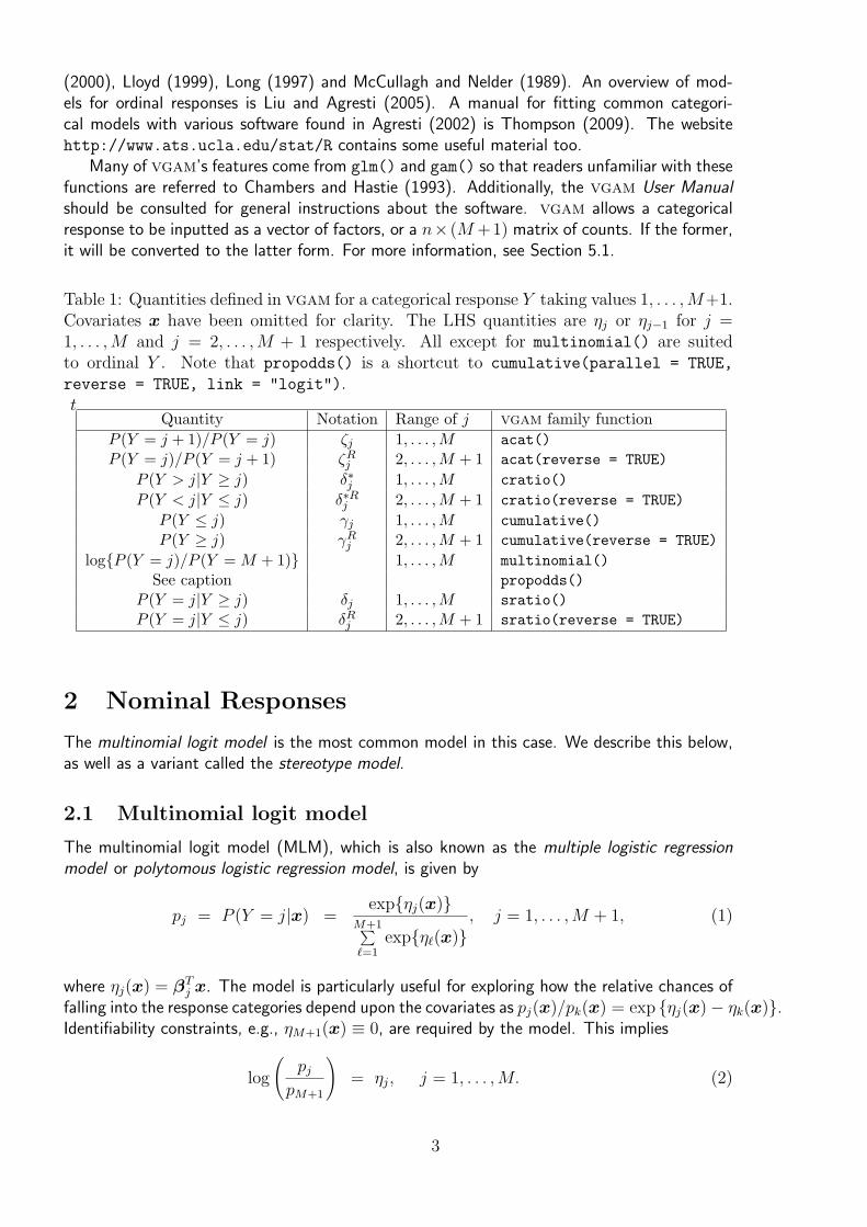
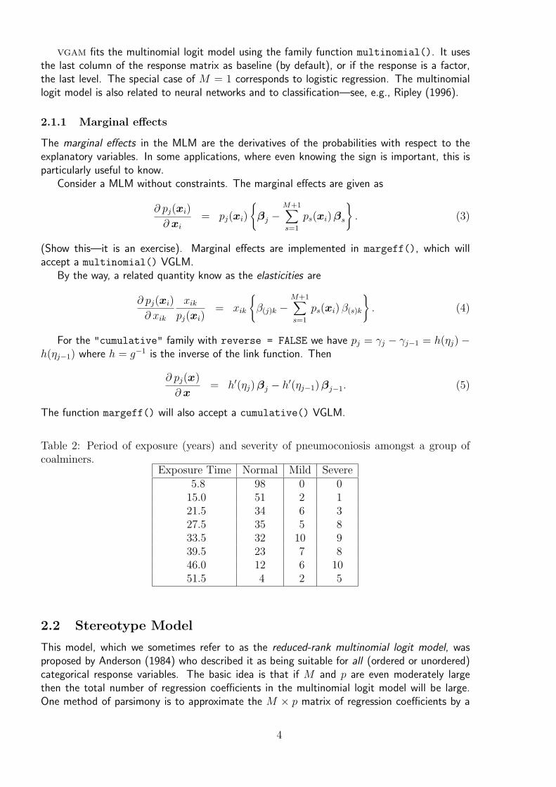
This document describes in detail vgam family functions for a categorical response variabletaking values Y = 1, 2, . . . ,M+1. Table 1 summarizes those current available. It is convenientto consider the two cases: when Y is nominal (no order) and when Y is ordinal (ordered). Anexample of the latter is Table 2 where the stages of a disease are Y = 1 for none, Y = 2 formild, and Y = 3 for severe symptoms.
Regarding further documentation, Yee (2010) is a journal article version complementingthis document and Yee (2008) gives an overview of VGLMs/VGAMs. General references forcategorical data include Simonoff (2003), Agresti (2002), Fahrmeir and Tutz (2001), Leonard
2
(2000), Lloyd (1999), Long (1997) and McCullagh and Nelder (1989). An overview of mod-els for ordinal responses is Liu and Agresti (2005). A manual for fitting common categori-cal models with various software found in Agresti (2002) is Thompson (2009). The websitehttp://www.ats.ucla.edu/stat/R contains some useful material too.
Many of vgam’s features come from glm() and gam() so that readers unfamiliar with thesefunctions are referred to Chambers and Hastie (1993). Additionally, the vgam User Manualshould be consulted for general instructions about the software. vgam allows a categoricalresponse to be inputted as a vector of factors, or a n× (M +1) matrix of counts. If the former,it will be converted to the latter form. For more information, see Section 5.1.
Table 1: Quantities defined in vgam for a categorical response Y taking values 1, . . . ,M+1.Covariates x have been omitted for clarity. The LHS quantities are ηj or ηj−1 for j =1, . . . ,M and j = 2, . . . ,M + 1 respectively. All except for multinomial() are suitedto ordinal Y . Note that propodds() is a shortcut to cumulative(parallel = TRUE,
reverse = TRUE, link = "logit").t
Quantity Notation Range of j vgam family functionP (Y = j + 1)/P (Y = j) ζj 1, . . . ,M acat()P (Y = j)/P (Y = j + 1) ζRj 2, . . . ,M + 1 acat(reverse = TRUE)
P (Y > j|Y ≥ j) δ∗j 1, . . . ,M cratio()P (Y < j|Y ≤ j) δ∗Rj 2, . . . ,M + 1 cratio(reverse = TRUE)
P (Y ≤ j) γj 1, . . . ,M cumulative()P (Y ≥ j) γRj 2, . . . ,M + 1 cumulative(reverse = TRUE)
log{P (Y = j)/P (Y = M + 1)} 1, . . . ,M multinomial()See caption propodds()
P (Y = j|Y ≥ j) δj 1, . . . ,M sratio()P (Y = j|Y ≤ j) δRj 2, . . . ,M + 1 sratio(reverse = TRUE)
2 Nominal Responses
The multinomial logit model is the most common model in this case. We describe this below,as well as a variant called the stereotype model.
2.1 Multinomial logit model
The multinomial logit model (MLM), which is also known as the multiple logistic regressionmodel or polytomous logistic regression model, is given by
pj = P (Y = j|x) =exp{ηj(x)}
M+1∑`=1
exp{η`(x)}, j = 1, . . . ,M + 1, (1)
where ηj(x) = βTj x. The model is particularly useful for exploring how the relative chances offalling into the response categories depend upon the covariates as pj(x)/pk(x) = exp {ηj(x)− ηk(x)}.Identifiability constraints, e.g., ηM+1(x) ≡ 0, are required by the model. This implies
log
(pj
pM+1
)= ηj, j = 1, . . . ,M. (2)
3
vgam fits the multinomial logit model using the family function multinomial(). It usesthe last column of the response matrix as baseline (by default), or if the response is a factor,the last level. The special case of M = 1 corresponds to logistic regression. The multinomiallogit model is also related to neural networks and to classification—see, e.g., Ripley (1996).
2.1.1 Marginal effects
The marginal effects in the MLM are the derivatives of the probabilities with respect to theexplanatory variables. In some applications, where even knowing the sign is important, this isparticularly useful to know.
Consider a MLM without constraints. The marginal effects are given as
∂ pj(xi)
∂ xi= pj(xi)
{βj −
M+1∑s=1
ps(xi)βs
}. (3)
(Show this—it is an exercise). Marginal effects are implemented in margeff(), which willaccept a multinomial() VGLM.
By the way, a related quantity know as the elasticities are
∂ pj(xi)
∂ xik
xikpj(xi)
= xik
{β(j)k −
M+1∑s=1
ps(xi) β(s)k
}. (4)
For the "cumulative" family with reverse = FALSE we have pj = γj − γj−1 = h(ηj)−h(ηj−1) where h = g−1 is the inverse of the link function. Then
∂ pj(x)
∂ x= h′(ηj)βj − h′(ηj−1)βj−1. (5)
The function margeff() will also accept a cumulative() VGLM.
Table 2: Period of exposure (years) and severity of pneumoconiosis amongst a group ofcoalminers.
Exposure Time Normal Mild Severe5.8 98 0 0
15.0 51 2 121.5 34 6 327.5 35 5 833.5 32 10 939.5 23 7 846.0 12 6 1051.5 4 2 5
2.2 Stereotype Model
This model, which we sometimes refer to as the reduced-rank multinomial logit model, wasproposed by Anderson (1984) who described it as being suitable for all (ordered or unordered)categorical response variables. The basic idea is that if M and p are even moderately largethen the total number of regression coefficients in the multinomial logit model will be large.One method of parsimony is to approximate the M × p matrix of regression coefficients by a
4
lower rank matrix. In detail, the reduced-rank concept replaces B = (β1, . . . ,βM)T (withoutthe intercepts) by
B = CAT (6)
where C = (c1 c2 · · · cr) is p × r, A = (a1 a2 · · ·ar) is M × r and r (usually � min(M, p))is the rank of A and C. It is convenient to write
ηi = η0 + A CTxi = η0 + Aνi .
The stereotype model is a special case of a Reduced-rank VGLM (RR-VGLM). It maybe fitted using rrvglm() and multinomial(). See the other documentation regarding RR-VGLMs for more details.
It is well known that the factorization (6) is not unique as ηi = η0 + A M M−1 νi for anynonsingular matrix M. A common form of constraint which ensures A is of rank r and uniqueis to restrict it to the form
A =
(IrA
),
where A is a (M − r) × r matrix. In fact, any r rows of A may be chosen to represent Ir1.
This method of identifiability is implemented in vgam.
3 Ordinal Responses
3.1 Models Involving Cumulative Probabilities
When the response is ordered the most common models involve the cumulative probabilitiesP (Y ≤ j|x) (see McCullagh (1980)), in particular, the proportional odds model is
logitP (Y ≤ j|x) = β(j)1 + βTx(−1), j = 1, . . . ,M.
We call models of the form
logitP (Y ≤ j|x) = ηj j = 1, . . . ,M
cumulative logit models as they involve the logit link function and cumulative probabilities.The proportional odds model is a cumulative logit model with the parallelism assumption β1 =· · · = βM . It is well-known that the parallelism assumption applied to a cumulative logit modelresults in the effect of the covariates on the odds ratio being the same regardless of the divisionpoint j, hence the name proportional odds model (this property is called strict stochasticordering (McCullagh, 1980)). In practice, the parallelism assumption should be checked; see,e.g., Armstrong and Sloan (1989), Peterson (1990). In general, the proportional odds model is
logitP (Y ≤ j|x) = β(j)1 + η, j = 1, . . . ,M. (7)
If a complementary log-log link is chosen in (7) the result is known as the proportional hazardsmodel. In theory, any other link function used for binomial data such as the probit link (which
1Actually, if the ‘wrong’ rows of A are chosen to represent Ir, then A may be ill-conditioned at thesolution, or even failing to exist.
5
is often referred to as the ordinal probit model or cumulative probit model) can be applied tocumulative probability models.
One reason for the proportional-odds cumulative-logit model’s popularity is its connectionto the idea of a continuous latent response. It can be shown that proportional-odds modelcan be motivated by the categorical outcome Y being a categorized version of an unobservable(latent) continuous variable, Z, say. Then Y = k if ck−1 < Z ≤ ck where the ck are known ascutpoints. It is assumed that the regression of Z on x has the form
Z = βTx+ ε,
where x has an intercept and ε is a random error from a logistic distribution with mean zero andconstant variance. Then the coarsened version Y will be related to the x by a proportional-oddscumulative logit model. Note that the logistic distribution has a bell-shaped density similar toa normal curve, and it may be fitted to raw data with vgam family functions logistic1()
and logistic2(). If ε had normal errors rather than logistic errors then the cumulative logitequations would change to have a probit link—this is known as a cumulative probit model. Formore information see McCullagh and Nelder (1989).
vgam fits models based on cumulative probabilities using the family function cumula-
tive(). It has a limited shortcut called propodds(). Liu and Agresti (2005) call this class ofmodels cumulative link models. Of course, cumulative() allows other link functions, and theparallelism assumption β1 = · · · = βM (or more generally, f(1)k(xk) = · · · = f(M)k(xk)). Forexample,
> vglm(y ~ x2, cumulative(link = probit, reverse = TRUE,
+ parallel = TRUE), mydataframe)
fits the model
Φ−1{P (Y ≥ j|x)} = β(j−1)1 + β2x2, j = 2, . . . ,M + 1.
Similarly,
> vgam(y ~ s(x2), cumulative(link = probit, reverse = TRUE,
+ parallel = TRUE), mydataframe)
fits the model
Φ−1{P (Y ≥ j|x)} = β(j−1)1 + f(1)2(x2), j = 2, . . . ,M + 1
for some smooth function f(1)2.If the proportional odds assumption is inadequate then one can try to use a different link
function or add extra terms such as interaction terms into the linear predictor. Another strategyis the so-called partial proportional odds model (Peterson and Harrell, 1990) which vgam mayfit.
3.2 Models Involving Stopping-ratios and Continuation-ratios
Quantities known as continuation-ratios are useful for the analysis of a sequential process, e.g.,to ascertain the effect of a covariate on the number of children a couple choose to have (Y = 1(no children), 2 (1 child), 3 (2 child), 4 (3+ children)), or whether a risk factor is related to theprogression of a disease (Y = 1 (no disease), 2 (localized), 3 (widespread), 4 (terminal)). Forsuch data, there are two ways of modelling the situation—these are deciding whether to look at
6
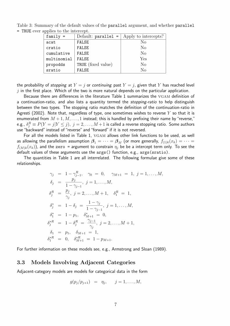
Table 3: Summary of the default values of the parallel argument, and whether parallel= TRUE ever applies to the intercept.
family = Default: parallel = Apply to intercepts?acat FALSE Nocratio FALSE Nocumulative FALSE Nomultinomial FALSE Yespropodds TRUE (fixed value) Nosratio FALSE No
the probability of stopping at Y = j or continuing past Y = j, given that Y has reached levelj in the first place. Which of the two is more natural depends on the particular application.
Because there are differences in the literature Table 1 summarizes the vgam definition ofa continuation-ratio, and also lists a quantity termed the stopping-ratio to help distinguishbetween the two types. The stopping ratio matches the definition of the continuation-ratio inAgresti (2002). Note that, regardless of type, one sometimes wishes to reverse Y so that it isenumerated from M + 1,M, . . . , 1 instead; this is handled by prefixing their name by“reverse,”e.g., δRj ≡ P (Y = j|Y ≤ j), j = 2, . . . ,M+1 is called a reverse stopping ratio. Some authorsuse “backward” instead of “reverse” and “forward” if it is not reversed.
For all the models listed in Table 1, vgam allows other link functions to be used, as wellas allowing the parallelism assumption β1 = · · · = βM (or more generally, f(1)k(xk) = · · · =f(M)k(xk)), and the zero = argument to constrain ηj be be a intercept term only. To see thedefault values of these arguments use the args() function, e.g., args(sratio).
The quantities in Table 1 are all interrelated. The following formulae give some of theserelationships.
γj = 1− γRj−1, γ0 = 0, γM+1 = 1, j = 1, . . . ,M,
δj =pj
1− γj−1
, j = 1, . . . ,M,
δRj =pjγj, j = 2, . . . ,M + 1, δR1 = 1,
δ∗j = 1− δj =1− γj
1− γj−1
, j = 1, . . . ,M,
δ∗1 = 1− p1, δ∗M+1 = 0,
δ∗Rj = 1− δRj =γj−1
γj, j = 2, . . . ,M + 1,
δ1 = p1, δM+1 = 1,
δ∗R1 = 0, δ∗RM+1 = 1− pM+1.
For further information on these models see, e.g., Armstrong and Sloan (1989).
3.3 Models Involving Adjacent Categories
Adjacent-category models are models for categorical data in the form
g(pj/pj+1) = ηj, j = 1, . . . ,M,
7
for some link function g (log or identity because pj/pj+1 does not necessarily lie in [0, 1].)Reverse adjacent-category models use
g(pj/pj−1) = ηj−1, j = 2, . . . ,M + 1.
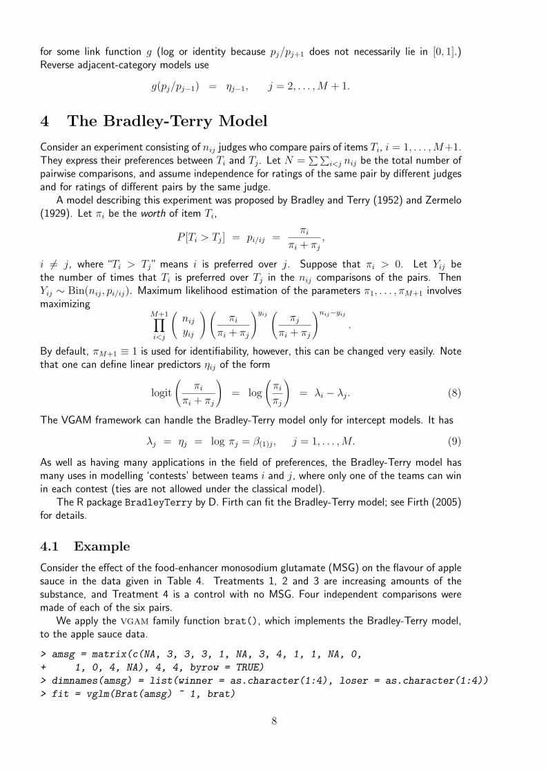
4 The Bradley-Terry Model
Consider an experiment consisting of nij judges who compare pairs of items Ti, i = 1, . . . ,M+1.They express their preferences between Ti and Tj. Let N =
∑∑i<j nij be the total number of
pairwise comparisons, and assume independence for ratings of the same pair by different judgesand for ratings of different pairs by the same judge.
A model describing this experiment was proposed by Bradley and Terry (1952) and Zermelo(1929). Let πi be the worth of item Ti,
P [Ti > Tj] = pi/ij =πi
πi + πj,
i 6= j, where “Ti > Tj” means i is preferred over j. Suppose that πi > 0. Let Yij bethe number of times that Ti is preferred over Tj in the nij comparisons of the pairs. ThenYij ∼ Bin(nij, pi/ij). Maximum likelihood estimation of the parameters π1, . . . , πM+1 involvesmaximizing
M+1∏i<j
(nijyij
)(πi
πi + πj
)yij(
πjπi + πj
)nij−yij
.
By default, πM+1 ≡ 1 is used for identifiability, however, this can be changed very easily. Notethat one can define linear predictors ηij of the form
logit
(πi
πi + πj
)= log
(πiπj
)= λi − λj. (8)
The VGAM framework can handle the Bradley-Terry model only for intercept models. It has
λj = ηj = log πj = β(1)j, j = 1, . . . ,M. (9)
As well as having many applications in the field of preferences, the Bradley-Terry model hasmany uses in modelling ‘contests’ between teams i and j, where only one of the teams can winin each contest (ties are not allowed under the classical model).
The R package BradleyTerry by D. Firth can fit the Bradley-Terry model; see Firth (2005)for details.
4.1 Example
Consider the effect of the food-enhancer monosodium glutamate (MSG) on the flavour of applesauce in the data given in Table 4. Treatments 1, 2 and 3 are increasing amounts of thesubstance, and Treatment 4 is a control with no MSG. Four independent comparisons weremade of each of the six pairs.
We apply the vgam family function brat(), which implements the Bradley-Terry model,to the apple sauce data.
> amsg = matrix(c(NA, 3, 3, 3, 1, NA, 3, 4, 1, 1, NA, 0,
+ 1, 0, 4, NA), 4, 4, byrow = TRUE)
> dimnames(amsg) = list(winner = as.character(1:4), loser = as.character(1:4))
> fit = vglm(Brat(amsg) ~ 1, brat)
8
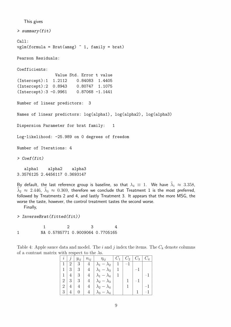
This gives
> summary(fit)
Call:
vglm(formula = Brat(amsg) ~ 1, family = brat)
Pearson Residuals:
Coefficients:
Value Std. Error t value
(Intercept):1 1.2112 0.84083 1.4405
(Intercept):2 0.8943 0.80747 1.1075
(Intercept):3 -0.9961 0.87068 -1.1441
Number of linear predictors: 3
Names of linear predictors: log(alpha1), log(alpha2), log(alpha3)
Dispersion Parameter for brat family: 1
Log-likelihood: -25.989 on 0 degrees of freedom
Number of Iterations: 4
> Coef(fit)
alpha1 alpha2 alpha3
3.3576125 2.4456117 0.3693147
By default, the last reference group is baseline, so that λ4 ≡ 1. We have λ1 ≈ 3.358,λ2 ≈ 2.446, λ3 ≈ 0.369, therefore we conclude that Treatment 1 is the most preferred,followed by Treatments 2 and 4, and lastly Treatment 3. It appears that the more MSG, theworse the taste, however, the control treatment tastes the second worse.
Finally,
> InverseBrat(fitted(fit))
1 2 3 4
1 NA 0.5785771 0.9009064 0.7705165
Table 4: Apple sauce data and model. The i and j index the items. The Ck denote columnsof a contrast matrix with respect to the λs.
i j yij nij ηij C1 C2 C3 C4
1 2 3 4 λ1 − λ2 1 –11 3 3 4 λ1 − λ3 1 –11 4 3 4 λ1 − λ4 1 –12 3 3 4 λ2 − λ3 1 –12 4 4 4 λ2 − λ4 1 –13 4 0 4 λ3 − λ4 1 –1
9
2 0.42142293 NA 0.8688013 0.7097758
3 0.09909362 0.1311987 NA 0.2697077
4 0.22948346 0.2902242 0.7302923 NA
gives the estimated probabilities of Treatments i“beating” Treatments j, P [i > j].
4.2 Bradley-Terry Model with Ties
Consider a Bradley-Terry model with ties (no preference). This is useful because it is commonfor people to say that both Ti and Tj are equally good or bad. There are at least two ways ofmodelling ties:
(i)
P (Ti > Tj) =πi
πi + πj + π0
,
P (Ti < Tj) =πj
πi + πj + π0
,
P (Ti = Tj) =π0
πi + πj + π0
.
Here, π0 > 0 is an extra parameter.
(ii) Davidson (1970) proposed
P (Ti > Tj) =πi
πi + πj + q√πi πj
,
P (Ti < Tj) =πj
πi + πj + q√πi πj
,
P (Ti = Tj) =q√πi πj
πi + πj + q√πi πj
,
where q > 1.
The first model, (i), has been implemented in the vgam family function bratt(). It has
η = (log π1, . . . , log πM−1, log π0)T
by default, where there are M competitors and πM ≡ 1. Like brat(), one can choose adifferent reference group and reference value.
For futher information about ties, see Kuk (1995) and Torsney (2004).
5 Other Topics
5.1 Input
The response in vglm()/vgam() can be
1. an n × (M + 1) matrix of counts. The columns are best labelled, and the jth columndenotes Y = j.
2. a vector. The unique values, when sorted (or levels if a factor), denote the M + 1 levelsfrom 1, . . . ,M + 1. If a factor, it may be ordered or unordered. The functions factor(),ordered(), levels(), are useful; see the R online help.
10
Note: if weights is used as input, then any zero values should be deleted first. For example,if n is a vector containing zeros, then something like
> vglm(..., weights = n, subset = n > 0)
should be used.
5.2 Output
Suppose fit is a categorical vgam object. Like binomialff(), the fitted values (in fit-
ted(fit)) are probabilities and weights(fit, type="prior") contain the ni =∑M+1j=1 yij.
However, fitted(fit) is a n× (M + 1) matrix, whose rows sum to unity.
5.3 Constraints
All categorical data family functions have the parallel and zero arguments. By default,parallel = FALSE and zero = NULL for all models. This means that to make the parallelismassumption one must explicitly invoke it as such. The reason for this is that the parallelismassumption must be checked, and the software discourages users from making assumptionswithout thinking. Unfortunately, the default values may fail on some data, or lead to a largenumber of parameters.
Table 3 summarizes whether parallel = TRUE is applied to the intercepts. Also, allcategorical data family functions have a reverse = FALSE argument.
5.4 Implementation Details
The S expression process.categorical.data.vgam provides a unified way of handling theresponse variable. The variable delete.zero.colns should be set to TRUE or FALSE prior toevaluating process.categorical.data.vgam in the slot @initialize to handle columns ofthe response matrix that contain all 0’s. In some situations these must be deleted.
Similarly, the expression deviance.categorical.data.vgam computes the deviance forall the models in this document.
5.5 Convergence
The vgam family functions described in this document use the type of algorithm describedin McCullagh (1980). He showed that a unique maximum of the likelihood is guarenteed forsufficiently large sample sizes, though infinite parameter values can arise with sparse data setscontaining certain patterns of zeros. Usually, one obtains rapid convergence to the MLEs.
5.6 Over-dispersion
Over-dispersion for polytomous responses can occur just like it does for binary responses (seedocumentation on GLM and GAM vgam family functions). Sec. 5.5 of McCullagh and Nelder(1989) use
σ2 = X2/{nM − p} = X2/{residual d.f}, (10)
where X2 is Pearson’s statistic. They state that this is approximately unbiased for σ2, isconsistent for large n regardless of whether the data are sparse, and is approximately independentof the estimated β.
11
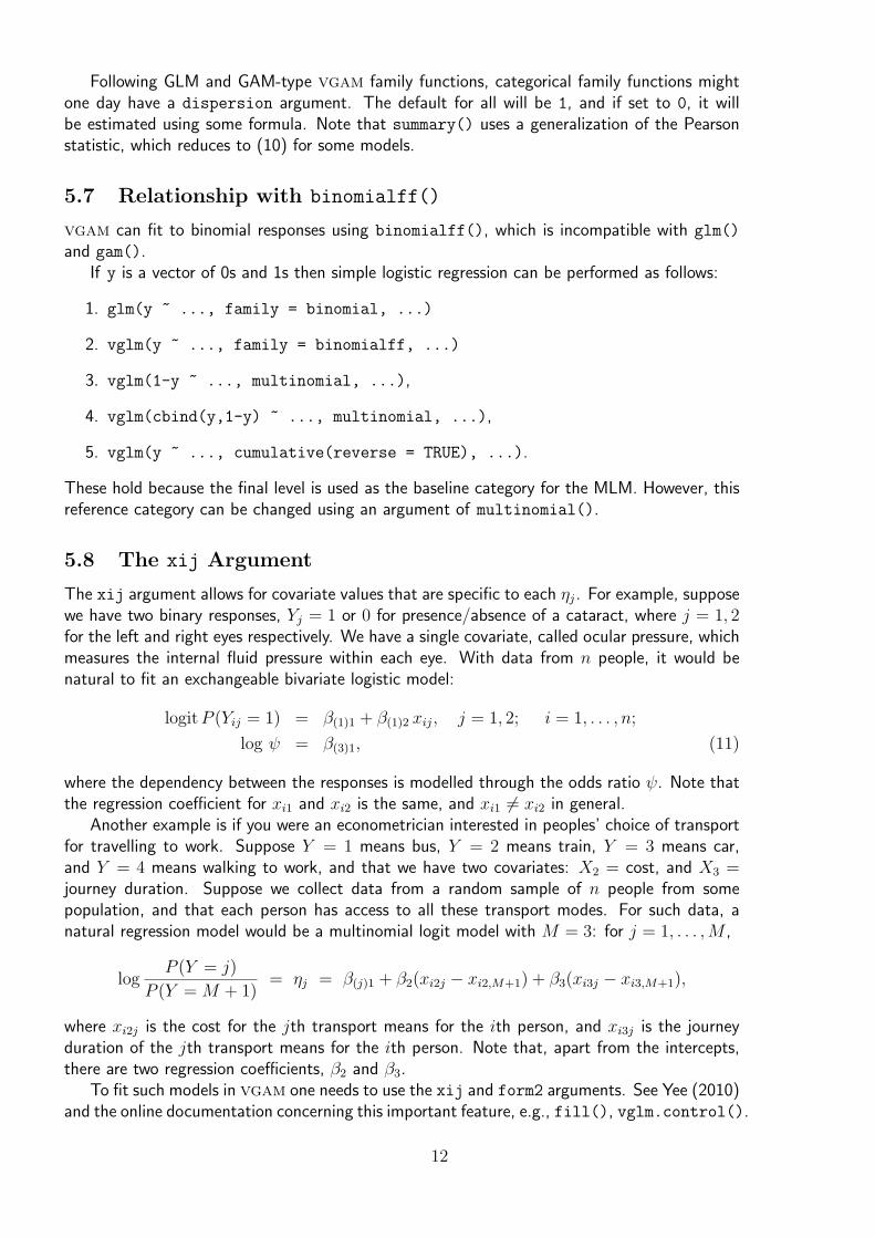
Following GLM and GAM-type vgam family functions, categorical family functions mightone day have a dispersion argument. The default for all will be 1, and if set to 0, it willbe estimated using some formula. Note that summary() uses a generalization of the Pearsonstatistic, which reduces to (10) for some models.
5.7 Relationship with binomialff()
vgam can fit to binomial responses using binomialff(), which is incompatible with glm()
and gam().If y is a vector of 0s and 1s then simple logistic regression can be performed as follows:
1. glm(y ~ ..., family = binomial, ...)
2. vglm(y ~ ..., family = binomialff, ...)
3. vglm(1-y ~ ..., multinomial, ...),
4. vglm(cbind(y,1-y) ~ ..., multinomial, ...),
5. vglm(y ~ ..., cumulative(reverse = TRUE), ...).
These hold because the final level is used as the baseline category for the MLM. However, thisreference category can be changed using an argument of multinomial().
5.8 The xij Argument
The xij argument allows for covariate values that are specific to each ηj. For example, supposewe have two binary responses, Yj = 1 or 0 for presence/absence of a cataract, where j = 1, 2for the left and right eyes respectively. We have a single covariate, called ocular pressure, whichmeasures the internal fluid pressure within each eye. With data from n people, it would benatural to fit an exchangeable bivariate logistic model:
logitP (Yij = 1) = β(1)1 + β(1)2 xij, j = 1, 2; i = 1, . . . , n;
log ψ = β(3)1, (11)
where the dependency between the responses is modelled through the odds ratio ψ. Note thatthe regression coefficient for xi1 and xi2 is the same, and xi1 6= xi2 in general.
Another example is if you were an econometrician interested in peoples’ choice of transportfor travelling to work. Suppose Y = 1 means bus, Y = 2 means train, Y = 3 means car,and Y = 4 means walking to work, and that we have two covariates: X2 = cost, and X3 =journey duration. Suppose we collect data from a random sample of n people from somepopulation, and that each person has access to all these transport modes. For such data, anatural regression model would be a multinomial logit model with M = 3: for j = 1, . . . ,M ,
logP (Y = j)
P (Y = M + 1)= ηj = β(j)1 + β2(xi2j − xi2,M+1) + β3(xi3j − xi3,M+1),
where xi2j is the cost for the jth transport means for the ith person, and xi3j is the journeyduration of the jth transport means for the ith person. Note that, apart from the intercepts,there are two regression coefficients, β2 and β3.
To fit such models in vgam one needs to use the xij and form2 arguments. See Yee (2010)and the online documentation concerning this important feature, e.g., fill(), vglm.control().
12
5.9 Reduced-rank Regression
A RR-VGLM (reduced-rank VGLM) replaces the (large) M ×p coefficient matrix BT by A CT ,where A is M × r and C is p × r, r � min(M, p). The application to the multinomial logitmodel is only one special case (called the stereotype model). For more details, see Yee andHastie (2003).
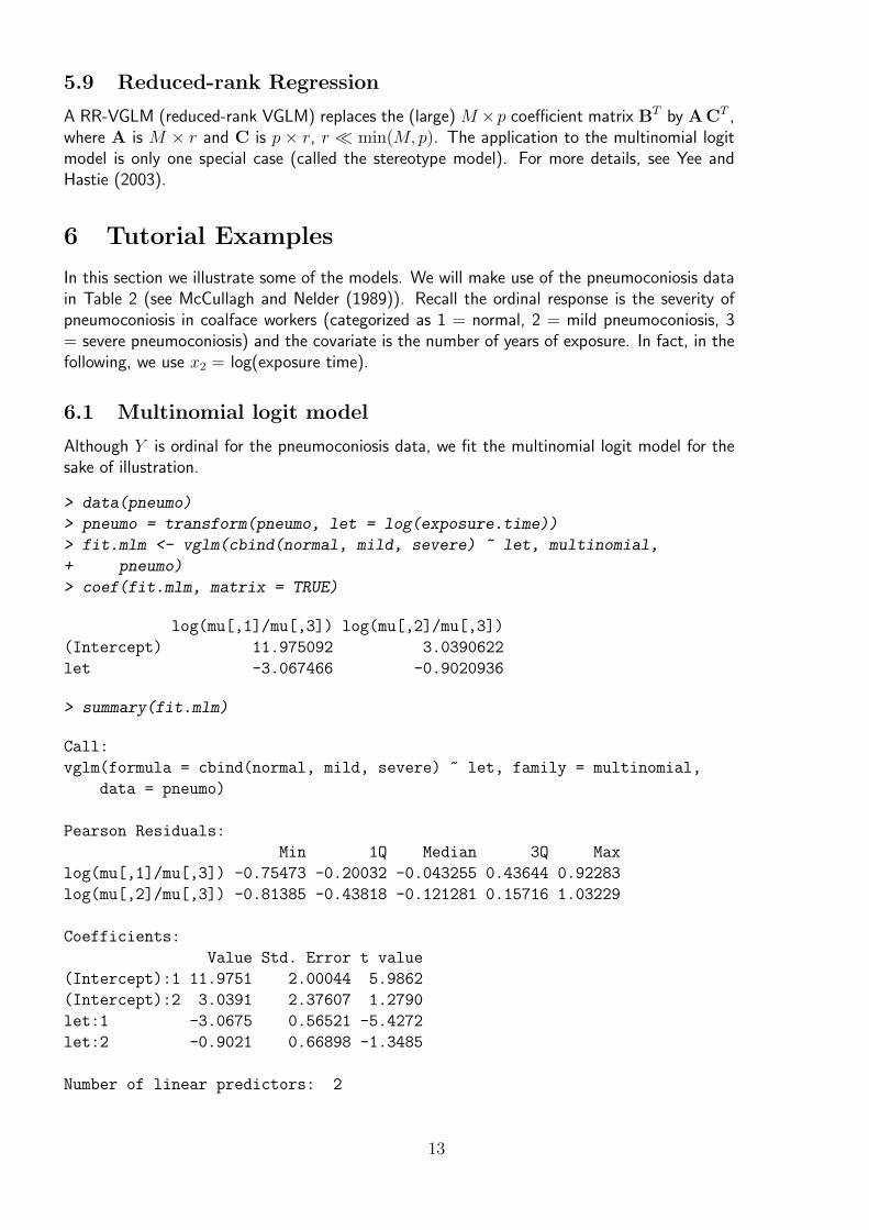
6 Tutorial Examples
In this section we illustrate some of the models. We will make use of the pneumoconiosis datain Table 2 (see McCullagh and Nelder (1989)). Recall the ordinal response is the severity ofpneumoconiosis in coalface workers (categorized as 1 = normal, 2 = mild pneumoconiosis, 3= severe pneumoconiosis) and the covariate is the number of years of exposure. In fact, in thefollowing, we use x2 = log(exposure time).
6.1 Multinomial logit model
Although Y is ordinal for the pneumoconiosis data, we fit the multinomial logit model for thesake of illustration.
> data(pneumo)
> pneumo = transform(pneumo, let = log(exposure.time))
> fit.mlm <- vglm(cbind(normal, mild, severe) ~ let, multinomial,
+ pneumo)
> coef(fit.mlm, matrix = TRUE)
log(mu[,1]/mu[,3]) log(mu[,2]/mu[,3])
(Intercept) 11.975092 3.0390622
let -3.067466 -0.9020936
> summary(fit.mlm)
Call:
vglm(formula = cbind(normal, mild, severe) ~ let, family = multinomial,
data = pneumo)
Pearson Residuals:
Min 1Q Median 3Q Max
log(mu[,1]/mu[,3]) -0.75473 -0.20032 -0.043255 0.43644 0.92283
log(mu[,2]/mu[,3]) -0.81385 -0.43818 -0.121281 0.15716 1.03229
Coefficients:
Value Std. Error t value
(Intercept):1 11.9751 2.00044 5.9862
(Intercept):2 3.0391 2.37607 1.2790
let:1 -3.0675 0.56521 -5.4272
let:2 -0.9021 0.66898 -1.3485
Number of linear predictors: 2
13
Names of linear predictors: log(mu[,1]/mu[,3]), log(mu[,2]/mu[,3])
Dispersion Parameter for multinomial family: 1
Residual Deviance: 5.34738 on 12 degrees of freedom
Log-likelihood: -25.25054 on 12 degrees of freedom
Number of Iterations: 4
Note that mu[j,] is the jth column of the matrix of fitted values. The estimated variance-covariance matrix of the regression coefficients is summary(fit.mlm)@cov.unscaled (if thedispersion parameter is unity), or more elegantly, vcov(fit.mlm).
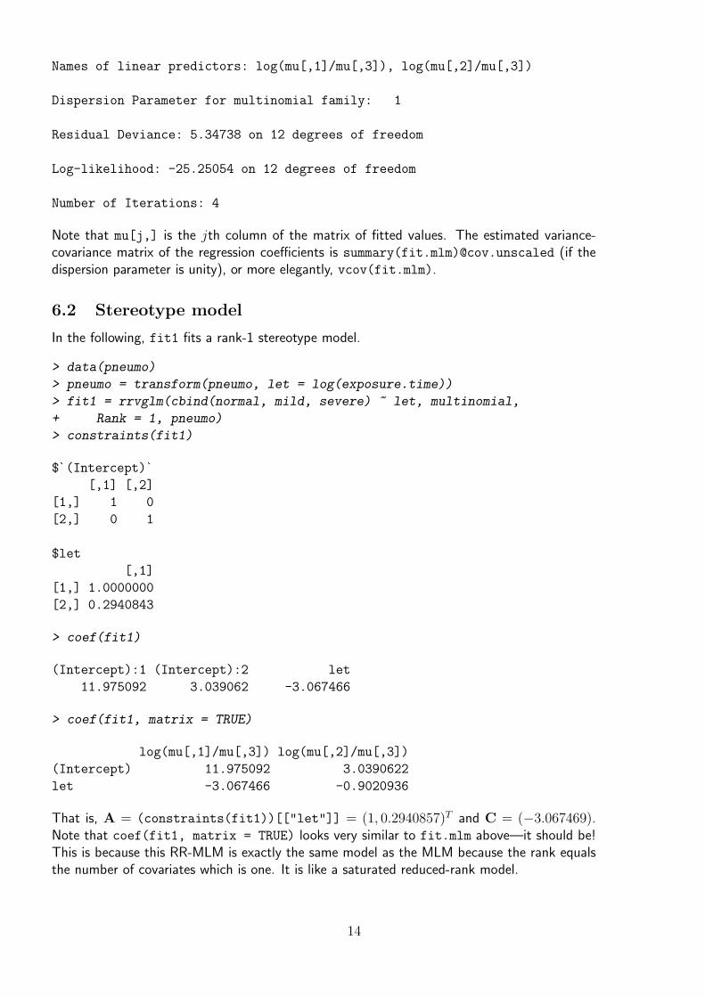
6.2 Stereotype model
In the following, fit1 fits a rank-1 stereotype model.
> data(pneumo)
> pneumo = transform(pneumo, let = log(exposure.time))
> fit1 = rrvglm(cbind(normal, mild, severe) ~ let, multinomial,
+ Rank = 1, pneumo)
> constraints(fit1)
$`(Intercept)`
[,1] [,2]
[1,] 1 0
[2,] 0 1
$let
[,1]
[1,] 1.0000000
[2,] 0.2940843
> coef(fit1)
(Intercept):1 (Intercept):2 let
11.975092 3.039062 -3.067466
> coef(fit1, matrix = TRUE)
log(mu[,1]/mu[,3]) log(mu[,2]/mu[,3])
(Intercept) 11.975092 3.0390622
let -3.067466 -0.9020936
That is, A = (constraints(fit1))[["let"]] = (1, 0.2940857)T and C = (−3.067469).Note that coef(fit1, matrix = TRUE) looks very similar to fit.mlm above—it should be!This is because this RR-MLM is exactly the same model as the MLM because the rank equalsthe number of covariates which is one. It is like a saturated reduced-rank model.
14
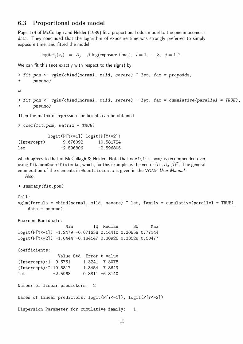
6.3 Proportional odds model
Page 179 of McCullagh and Nelder (1989) fit a proportional odds model to the pneumoconiosisdata. They concluded that the logarithm of exposure time was strongly preferred to simplyexposure time, and fitted the model
logit γj(xi) = αj − β log(exposure timei), i = 1, . . . , 8, j = 1, 2.
We can fit this (not exactly with respect to the signs) by
> fit.pom <- vglm(cbind(normal, mild, severe) ~ let, fam = propodds,
+ pneumo)
or
> fit.pom <- vglm(cbind(normal, mild, severe) ~ let, fam = cumulative(parallel = TRUE),
+ pneumo)
Then the matrix of regression coefficients can be obtained
> coef(fit.pom, matrix = TRUE)
logit(P[Y<=1]) logit(P[Y<=2])
(Intercept) 9.676092 10.581724
let -2.596806 -2.596806
which agrees to that of McCullagh & Nelder. Note that coef(fit.pom) is recommended overusing fit.pom@coefficients, which, for this example, is the vector (α1, α2, β)T . The generalenumeration of the elements in @coefficients is given in the vgam User Manual.
Also,
> summary(fit.pom)
Call:
vglm(formula = cbind(normal, mild, severe) ~ let, family = cumulative(parallel = TRUE),
data = pneumo)
Pearson Residuals:
Min 1Q Median 3Q Max
logit(P[Y<=1]) -1.2479 -0.071638 0.14410 0.30859 0.77144
logit(P[Y<=2]) -1.0444 -0.184147 0.30926 0.33528 0.50477
Coefficients:
Value Std. Error t value
(Intercept):1 9.6761 1.3241 7.3078
(Intercept):2 10.5817 1.3454 7.8649
let -2.5968 0.3811 -6.8140
Number of linear predictors: 2
Names of linear predictors: logit(P[Y<=1]), logit(P[Y<=2])
Dispersion Parameter for cumulative family: 1
15
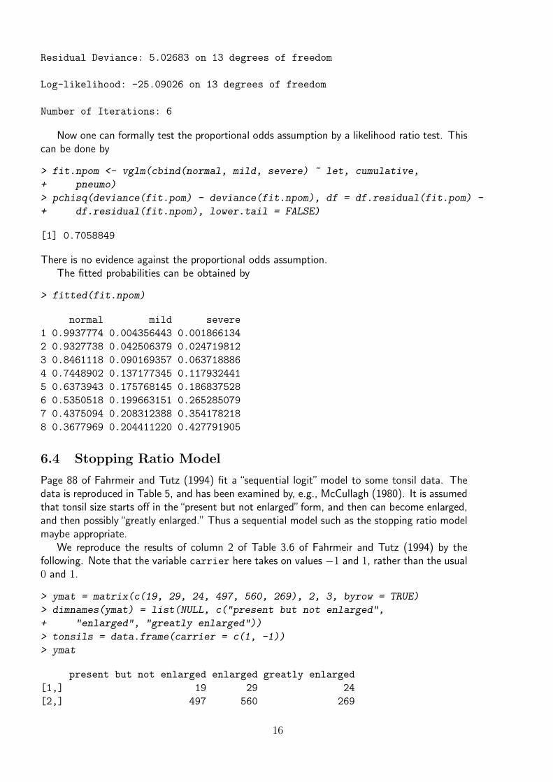
Residual Deviance: 5.02683 on 13 degrees of freedom
Log-likelihood: -25.09026 on 13 degrees of freedom
Number of Iterations: 6
Now one can formally test the proportional odds assumption by a likelihood ratio test. Thiscan be done by
> fit.npom <- vglm(cbind(normal, mild, severe) ~ let, cumulative,
+ pneumo)
> pchisq(deviance(fit.pom) - deviance(fit.npom), df = df.residual(fit.pom) -
+ df.residual(fit.npom), lower.tail = FALSE)
[1] 0.7058849
There is no evidence against the proportional odds assumption.The fitted probabilities can be obtained by
> fitted(fit.npom)
normal mild severe
1 0.9937774 0.004356443 0.001866134
2 0.9327738 0.042506379 0.024719812
3 0.8461118 0.090169357 0.063718886
4 0.7448902 0.137177345 0.117932441
5 0.6373943 0.175768145 0.186837528
6 0.5350518 0.199663151 0.265285079
7 0.4375094 0.208312388 0.354178218
8 0.3677969 0.204411220 0.427791905
6.4 Stopping Ratio Model
Page 88 of Fahrmeir and Tutz (1994) fit a “sequential logit” model to some tonsil data. Thedata is reproduced in Table 5, and has been examined by, e.g., McCullagh (1980). It is assumedthat tonsil size starts off in the“present but not enlarged”form, and then can become enlarged,and then possibly“greatly enlarged.” Thus a sequential model such as the stopping ratio modelmaybe appropriate.
We reproduce the results of column 2 of Table 3.6 of Fahrmeir and Tutz (1994) by thefollowing. Note that the variable carrier here takes on values −1 and 1, rather than the usual0 and 1.
> ymat = matrix(c(19, 29, 24, 497, 560, 269), 2, 3, byrow = TRUE)
> dimnames(ymat) = list(NULL, c("present but not enlarged",
+ "enlarged", "greatly enlarged"))
> tonsils = data.frame(carrier = c(1, -1))
> ymat
present but not enlarged enlarged greatly enlarged
[1,] 19 29 24
[2,] 497 560 269
16
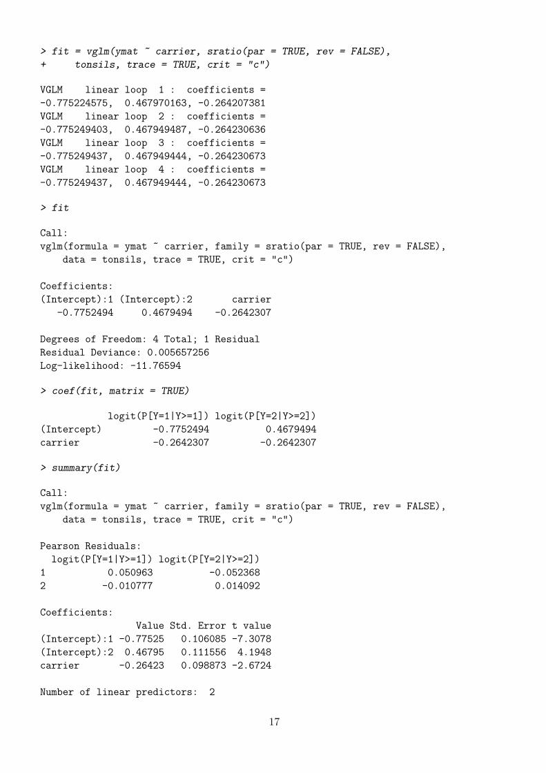
> fit = vglm(ymat ~ carrier, sratio(par = TRUE, rev = FALSE),
+ tonsils, trace = TRUE, crit = "c")
VGLM linear loop 1 : coefficients =
-0.775224575, 0.467970163, -0.264207381
VGLM linear loop 2 : coefficients =
-0.775249403, 0.467949487, -0.264230636
VGLM linear loop 3 : coefficients =
-0.775249437, 0.467949444, -0.264230673
VGLM linear loop 4 : coefficients =
-0.775249437, 0.467949444, -0.264230673
> fit
Call:
vglm(formula = ymat ~ carrier, family = sratio(par = TRUE, rev = FALSE),
data = tonsils, trace = TRUE, crit = "c")
Coefficients:
(Intercept):1 (Intercept):2 carrier
-0.7752494 0.4679494 -0.2642307
Degrees of Freedom: 4 Total; 1 Residual
Residual Deviance: 0.005657256
Log-likelihood: -11.76594
> coef(fit, matrix = TRUE)
logit(P[Y=1|Y>=1]) logit(P[Y=2|Y>=2])
(Intercept) -0.7752494 0.4679494
carrier -0.2642307 -0.2642307
> summary(fit)
Call:
vglm(formula = ymat ~ carrier, family = sratio(par = TRUE, rev = FALSE),
data = tonsils, trace = TRUE, crit = "c")
Pearson Residuals:
logit(P[Y=1|Y>=1]) logit(P[Y=2|Y>=2])
1 0.050963 -0.052368
2 -0.010777 0.014092
Coefficients:
Value Std. Error t value
(Intercept):1 -0.77525 0.106085 -7.3078
(Intercept):2 0.46795 0.111556 4.1948
carrier -0.26423 0.098873 -2.6724
Number of linear predictors: 2
17
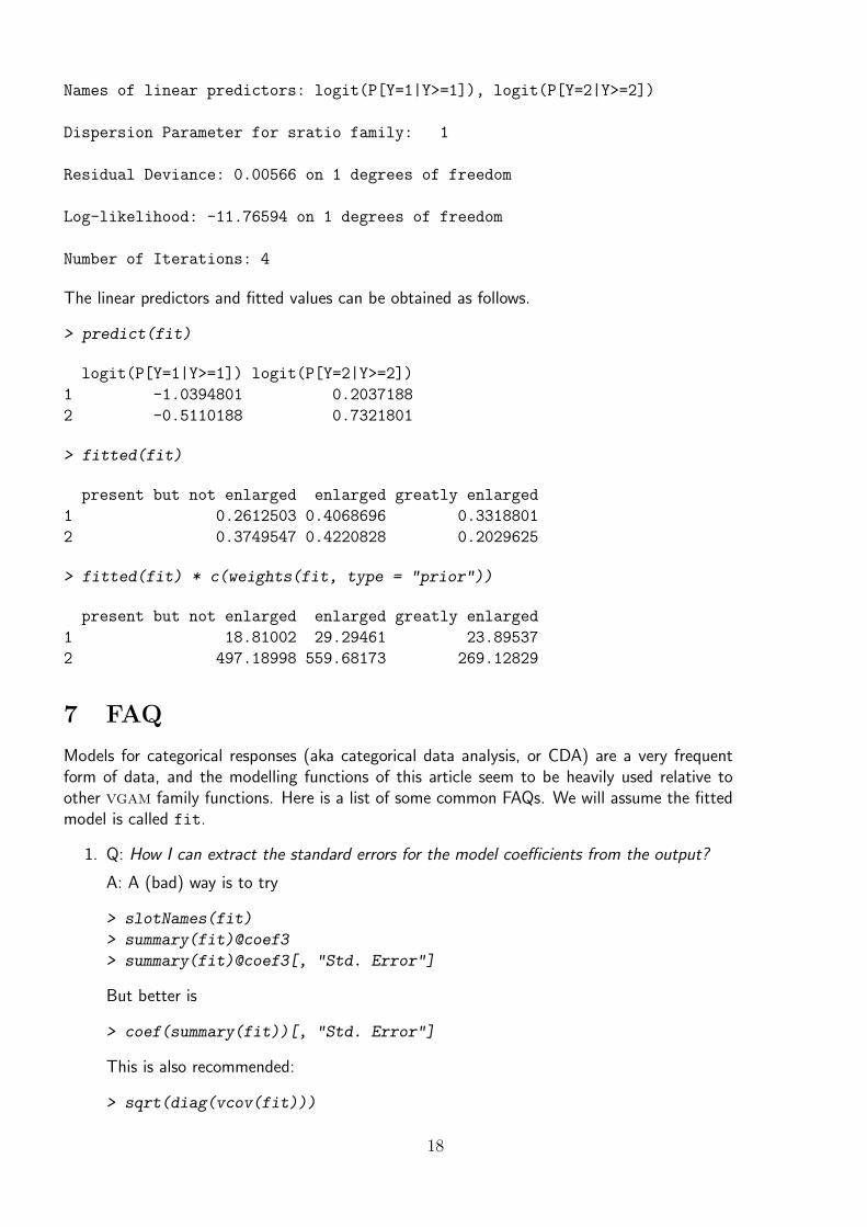
Names of linear predictors: logit(P[Y=1|Y>=1]), logit(P[Y=2|Y>=2])
Dispersion Parameter for sratio family: 1
Residual Deviance: 0.00566 on 1 degrees of freedom
Log-likelihood: -11.76594 on 1 degrees of freedom
Number of Iterations: 4
The linear predictors and fitted values can be obtained as follows.
> predict(fit)
logit(P[Y=1|Y>=1]) logit(P[Y=2|Y>=2])
1 -1.0394801 0.2037188
2 -0.5110188 0.7321801
> fitted(fit)
present but not enlarged enlarged greatly enlarged
1 0.2612503 0.4068696 0.3318801
2 0.3749547 0.4220828 0.2029625
> fitted(fit) * c(weights(fit, type = "prior"))
present but not enlarged enlarged greatly enlarged
1 18.81002 29.29461 23.89537
2 497.18998 559.68173 269.12829
7 FAQ
Models for categorical responses (aka categorical data analysis, or CDA) are a very frequentform of data, and the modelling functions of this article seem to be heavily used relative toother vgam family functions. Here is a list of some common FAQs. We will assume the fittedmodel is called fit.
1. Q: How I can extract the standard errors for the model coefficients from the output?
A: A (bad) way is to try
> slotNames(fit)
> summary(fit)@coef3
> summary(fit)@coef3[, "Std. Error"]
But better is
> coef(summary(fit))[, "Std. Error"]
This is also recommended:
> sqrt(diag(vcov(fit)))
18

Note that the slot name“coef3”may change in the future so it shouldn’t be used directly.
2. Q: Why aren’t the Wald statistics p-values printed out in the summary()?
A: vgam fits so many models from a broad range of statistical fields and subjects that itis potentially dangerous to print out a p-value. The methods function summaryvglm()
ought to be accurate for all vgam family functions, therefore it was thought that it wasbest to leave out p-values. Possibly an argument pvalues could be added in the future.
8 Other Software
There are several other R implementations for fitting categorical regression models. Some ofthem are described in Yee (2010), who argues that these implementations tend to be piecemealin nature, and do not provide a unified framework that is as understandable or comprehensiveas VGLMs/VGAMs.
9 Yet To Do
Things yet to be done include
1. Allow for a dispersion parameter. Currently this is possible for GLM-type family functions.A unified and uniform way of handling these is to have dispersion=0 or dispersion=1.It is easy to modify existing vgam family functions, but this hasn’t been done yet—thetheory is undeveloped.
2. Improvement to biplots of RR-VGLMs are needed.
3. RR-VGAMs are yet to be implemented. This involves vector projection pursuit regression.
4. Investigate vector smoothing subject to the constraint that the component functions neverintersect. This would mean the non-parametric cumulative logit model would not haveproblems with negative probabilities etc.
Exercises
1. McCullagh (1980) proposed the following model which incorporates dispersion effects:
P (Y ≤ j|x) = G
(β(j)0 − βTx
τx
),
where G is the cumulative distribution function of some continuous distribution such asthe logistic distribution. Write a vgam family function to fit this model. It should havethe usual parallel and reverse and zero options.
Table 5: Tonsil data. The size of the tonsil is cross-classified as to whether the child wasa carrier of Streptococcus pyogenes. The data was collected from 2413 healthy children(Holmes and Williams, 1954).
Carrier? Present but not enlarged Enlarged Greatly enlargedYes 19 29 24No 497 560 269
19
2. For the multinomial logit model show that Fisher scoring is equivalent to Newton-Raphson. To do this, show that the likelihood score vector di = ni(y
∗i − p∗i ), and
Wi = ni(diag(p∗i ) − p∗ip∗Ti ), where y∗i = (yi1, . . . , yiM)T are sample proportions,ni =
∑M+1j=1 yij is the number of counts with xi, and pi = (pi1, . . . , piM)T = E(y∗i ) are
fitted probabilities. The asterix here is used to denote that y∗i is yi with yi,M+1 dropped.Here, di = ∂`i/∂ηi, ` =
∑ni=1 `i is the log-likelihood, and Wi = −∂2`i/(∂η ∂η
T ).
3. Obtain an expression for the marginal effects of a cumulative logit model, cf. (3) for theMLM. Modify margeff() to compute this quantity for a cumulative() VGLM.
4. Motivate the Bradley-Terry model using a latent variable argument that uses the logisticdistribution. Replacing the logistic distribution by a normal distribution results in theThurstone model (i.e., replace the logit link in (8) by a probit link). Adapt brat() tohandle both distributions. Is it feasible to handle the cloglog() and tanl() links aswell? If so, implement those too.
5. Another way of modelling paired comparison data is via the model (Rao and Kupper,1967)
P (Ti > Tj) = πi/(πi + qπj),
P (Ti < Tj) = πj/(πj + qπi),
where q > 1. This model can be motivated by latent variables and a logistic distributionsince P (Ti > Tj) = G(λi−λj−τ), τ ≥ 0, where G(·) is the logistic distribution functionand πi = exp(λi), q = exp(τ).
6. Write a vgam family function to implement the model (ii) for ties in Section 4.2. It isbased on Davidson (1970).
7. Write a vgam family function to implement triple comparisons, i.e., let
θijk = P (Ti > Tj > Tk)
be the probability that Ti is preferred to Tj and Tj is preferred to Tk. One way is tochoose
θijk =πiπj
(πi + πj + πk)(πj + πk).
An alternative is
θijk =π2i πj
π2i πj + π2
jπi + π2i πk + π2
kπi + π2jπk + π2
kπj.
Write a vgam family function for each of these models.
8. Run the help-file example of the family function brat(). Show that the working residualsare all zero (or zero to working precision, depending on the convergence criterion—canyou get the model to iterate even closer to the MLE?). Explain the theory behind whythis is to be expected. Are Pearson residuals defined when the working residuals are allzero? Should summary.vglm() print out the working residuals if the Pearson residualsare undefined?
20
9. (a) Consider the standard random utility maximization model (RUM), with an indirectutility function given by
Uij = ηij + εij (12)
with i = 1, . . . , n and j = 1, . . . , J . Then Uij is the utility that individual igains from outcome j. Let the observed individual characteristics be xi and thecharacteristics of the outcomes be zij, then
ηij = xTi βj + zTijα. (13)
Finally, εij in (12) is assumed to follow an independent extreme value distribution.The probability that individual i selects outcome j is given by
Pij = P [Uij = max(Ui1, . . . , UiJ)]
with choice set C = {1, 2, . . . , J}, and associated multinomial logit model proba-bilities given by
Pmij =
exp(ηij)∑Jk=1 exp(ηik)
. (14)
(b) Write a vgam family function called dogit() to implement the dogit model. Thefollowing description comes from Fry and Harris (2005). The multinomial logitmodel imposes some strong restrictions on the model, most notably that of theindependence of irrelevant alternatives (IIA). The IIA property of the MLM saysthat the odds ratio Pij/Pik, j 6= k, is independent of all other alternatives, andindependent of additions to, and deletions from, the full choice set. This can be anunrealistic assumption.
Of the several non-IIA alternatives to the MLM proposed, the dogit model of Gaudryand Dagenais (1979) is attractive. The dogit model expands on (14) by having
P dij =
exp(ηij) + θj∑Jk=1 exp(ηik)(
1 +∑Jk=1 θk
)∑Jk=1 exp(ηik)
. (15)
Here, θj ≥ 0 for j = 1, . . . , J . This can be motivated by a two-part choice process(Fry and Harris, 1996).
Nb. Gaudry and Dagenais (1979) say that the IIA property of a model requires thatthe relative probabilities of any two alternatives be independent of the attributesof the remaining alternatives whether the latter are present or absent from theset of available choices. This property, introduced by Luce (1959) to explain thepsychology of choice, was used by McFadden (1968) to derive the multinomial logitmodel within a different theoretical framework. Gaudry and Dagenais (1979) call itthe “dogit” model because “the model avoids or dodges the researcher’s dilemma ofchoosing a priori between a format which commits to IIA restrictions and one whichexcludes them—whence its name.”
(c) Write a vgam family function called ogev() to implement the standard orderedGEV model, whose probabilities are given by
P oij =
ξij((ξi,j−1 + ξij)
ρ−1 + (ξij + ξi,j+1)ρ−1)
∑J+1r=1 (ξi,r−1 + ξir)
ρ (16)
where ξij = exp(ηij/ρ) with the ηij given by (13), ξi0 = ξi,J+1 = 0 and 0 < ρ ≤ 1.
21
(d) Write a vgam family function called dogev() to implement the DOGEV (dogitordered GEV) model whose probabilities are
PDij =
θj
1 +∑Mk=1 θk
+P oij
1 +∑Mk=1 θk
. (17)
Note that in all models, the log-likelihood function is
`k(φ) =n∑i=1
J∑j=1
dij logP kij
with k = m, d, o,D and model parameter vector φ = (β,α), (β,α,θ), (β,α, ρ),and (β,α,θ, ρ) respectively, where β = (β1, . . . ,βJ). Here, dij = 1 if individual ichooses outcome j, else dij = 0. Of course, one should use the zero argument tomake ρ intercept-only by default.
(e) Show that
P dij =
θj
1 +∑Jk=1 θk
+Pmij
1 +∑Jk=1 θk
.
References
Agresti, A., 2002. Categorical Data Analysis, 2nd Edition. Wiley, New York, USA.
Anderson, J. A., 1984. Regression and ordered categorical variables. Journal of the Royal Sta-tistical Society. Series B 46 (1), 1–30, with discussion.
Armstrong, B. G., Sloan, M., 1989. Ordinal regression models for epidemiologic data. AmericanJournal of Epidemiology 129, 191–204.
Bradley, R. A., Terry, M. E., 1952. Rank analysis of incomplete block designs. I. The methodof paired comparisons. Biometrika 39, 324–345.
Chambers, J. M., Hastie, T. J. (Eds.), 1993. Statistical Models in S. Chapman & Hall, NewYork, USA.
Davidson, R. R., 1970. On extending the Bradley Terry model to accommodate ties in pairedcomparison experiments. J. Amer. Statist. Assoc. 65, 317–328.
Fahrmeir, L., Tutz, G., 1994. Multivariate Statistical Modelling Based on Generalized LinearModels. Springer-Verlag.
Fahrmeir, L., Tutz, G., 2001. Multivariate Statistical Modelling Based on Generalized LinearModels, 2nd Edition. Springer-Verlag, New York, USA.
Firth, D., 2005. Bradley-Terry models in R. Journal of Statistical Software 12 (1), 1–12.
Fry, T. R. L., Harris, M., 1996. A Monte Carlo study of tests for the independence of irrelevantalternatives property. Transportation Research, Part B 30B (1), 19–30.
Fry, T. R. L., Harris, M. N., 2005. The dogit ordered generalized extreme value model. TheAustralian and New Zealand Journal of Statistics 47 (4), 531–542.
22
Gaudry, M., Dagenais, M., 1979. The dogit model. Transportation Research, Part B 13B (2),105–112.
Holmes, M. C., Williams, R., 1954. The distribution of carriers of Streptococcus Pyogenesamongst 2413 healthy children. J. Hyg. Camb. 52, 165–179.
Kuk, A. Y. C., 1995. Modelling paired comparison data with large numbers of draws and largevariability of draw percentage among players. The Statistician 44, 523–528.
Leonard, T., 2000. A Course in Categorical Data Analysis. Chapman & Hall/CRC, Boca Raton,FL, USA.
Liu, I., Agresti, A., 2005. The analysis of ordered categorical data: An overview and a surveyof recent developments. Sociedad Estadıstica e Investigacion Operativa Test 14 (1), 1–73.
Lloyd, C. J., 1999. Statistical Analysis of Categorical Data. Wiley, New York, USA.
Long, J. S., 1997. Regression Models for Categorical and Limited Dependent Variables. SagePublications, Thousand Oaks, CA, USA.
Luce, R. D., 1959. Individual Choice Behavior. Wiley, New York, USA.
McCullagh, P., 1980. Regression models for ordinal data. J. Roy. Statist. Soc. Ser. B 42 (2),109–142.
McCullagh, P., Nelder, J. A., 1989. Generalized Linear Models, 2nd Edition. Chapman & Hall,London.
McFadden, D., 1968. The revealed preferences of a government bureaucracy. Tech. Rep. 17,Department of Economics, University of California.
Peterson, B., 1990. Letter to the editor: Ordinal regression models for epidemiologic data.American Journal of Epidemiology 131, 745–746.
Peterson, B., Harrell, F. E., 1990. Partial proportional odds models for ordinal response variables.Applied Statistics 39 (2), 205–217.
Rao, P. V., Kupper, L. L., 1967. Ties in paired comparison experiments: a generalisation of theBradley Terry. J. Amer. Statist. Assoc. 62, 192–204.
Ripley, B. D., 1996. Pattern Recognition and Neural Networks. Cambridge University Press,Cambridge.
Simonoff, J. S., 2003. Analyzing Categorical Data. Springer-Verlag, New York, USA.
Thompson, L. A., 2009. R (and S-PLUS) Manual to Accompany Agresti’s Categorical DataAnalysis (2002), 2nd edition.URL https://home.comcast.net/~lthompson221/Splusdiscrete2.pdf
Torsney, B., 2004. Fitting Bradley Terry models using a multiplicative algorithm. In: Antoch,J. (Ed.), Proceedings in Computational Statistics COMPSTAT 2004. Physica-Verlag, Heidel-berg, pp. 513–526.
Yee, T. W., 2008. The vgam package. R News 8 (2), 28–39.URL http://CRAN.R-project.org/doc/Rnews/
23

Yee, T. W., 2010. The VGAM package for categorical data analysis. Journal of StatisticalSoftware 32 (10), 1–34.URL http://www.jstatsoft.org/v32/i10/
Yee, T. W., Hastie, T. J., 2003. Reduced-rank vector generalized linear models. StatisticalModelling 3 (1), 15–41.
Zermelo, E., 1929. Die berechnung turnier-ergebnisse als ein maximumproblem der wahrschein-lichkeitsrechnung. Math. Zeit. 29, 436–460.
24