AD-A127 498 VESSEL NAVIGATION SYSTEM SIMULATION VOLUME I TECHNICAL 1/1DESCRIPTION(U) DELTA RESEARCH INC HUNTSVILLE ALL B WEINER JAN 82 DR-083-282 USCG-D-Bi-82

UNCLASSIFIED DTCG2-88-D-28036 F/G 17/7 N

I"% . . . . . . . .. . . - . -. ..... ; - - -

.4

|1.0Wlull . ~ * ,. i.-- -

fill'-

1111 WoI~ 12.0

1.2 LAL.

MICROCOPY RESOLUTION TEST CHARTftAIDNAI. BUREAU OF STANDADS-j6 3 _A

. . . .... . . . . ..V . . . . ... . .. . . * . % . . . * . . ,. ..A

|' .,. ,..'.... .. ,.'.... .,. .-.-. ...- '.,.',. , . ". '" A .',-" . . .. .. . . "- .. . ,-:-' .'.,.:,_',-,L', '_-,.:& .'-L --. '..,."',-. - - . . '..-" . ,.'.'...,.A .A ", A . -A. , - "A,

Report No. CG-D-01-82

VESSEL NAVIGATION SYSTEM SIMULATION

VOLUME I: TECHNICAL DESCRIPTION

I

DELTA RESEARCH, INC.2109 WEST CLINTON AVENUE

SUITE 414HUNTSVILLE, ALABAMA 35805

FINAL REPORT

JANUARY 1982

Document is available to the public through theNational Technical Information Service, 4

Springfield, Virginia 22151 °(" .

Al 71 I'933

Prepared for A

* - U.S. DEPARTMENT OF TRANSPORTATIONUnited States Coast Guard

Office of Research and Development__j Washington, D.C. 20590

88 04 27 011,

NOTICE

This document is disseminated under the sponsorship of the Departmentof Transportation in the interest of information exchange. The UnitedSte Government assumes no liability for its connts or use thereof.

The contents of this report do not necessrilv reflect the official viewor policy of the Coast Guard; and they do not constitute a standard,specification, or regulation.

This report, or portions thereof may not be used for advertising orsales promotion purposes. Citation of trade names and manufacturersdoes not constitM endorsement or approval of such products.

mI

TecabeuIsteftqf Decomoateutees Page

Rptme . .6ermm.. Accession No. 3. Reipient's C;M'ee .

January 19826. Peeforinag Orgeaiation Cede

Vessel Navigation System SimulationVolume 1: Technical Description a. P~veroming Oegenis~eet Roer m.

* .Age.s) Delta Research, Inc.Louis B. Weiner 003-202

9. Poensimng Organiation Name and Address 10. Work Wit' Me. (TKAIS)

Delta Research, Inc.______________2109 W. Clinton Ave. 11. Contrast or Giant N.

Suite 414 DTCG2 3-8O-M2Ofl 6Huntsville, AL 35805 13. Type of Report and Period Ceveced

12. ponorig AgncyNom endAddtssFinal Report, SeptemberUnited States Coast Guard 1980 - December 1981Office of Research and Deeomet1. Sponsoring Agiency Cede

Washingtton. D.C. 20 5 9 0Deeomn G-DMT-1/54 ________

Is. Su.piemensry Noes.

(The technical representative for this contract was Dr. Ping Chuany,* 16 Abstract

T-6This Final Report discusses the mathematical formulation, computer program* implementation, and examples of the Vessel Navigation System Simulation (VNSS).

The VNSS simulates piloting a vessel in a restricted waterway, with channel banks,current, and obstacles. The techniques of modern optimal control theory is used

-* to derive the control history and resultant vessel trackline, using USCG suppliedcode definition for vehicle dynamics.

17. Kery Weeds Is. Distribution Staement" This Volume is availablito the U.S. public through:

Navigation National Technical Information ServiceSimulation Springfield, Virginia 22161optimal ControlCollision,_Ramming,_GroundingRisks ______________________

It. Securiy Clessif. lef th0is report) 30. S~wrt Ci...d. (of ON$s 11411) 2.No. *6 Peg to2.Pe

UNCLASSIFIED IUNCLASSIFIED 57 IPews DOT F 1700.7 (8-72) Reproduction of completed poe. eutheel ed

4

TABLE OF CONTENTS

Section Page

LIST OF FIGURES iiLIST OF TABLES iii

2. MATHEMATICAL REPRESENTATION 2-1

2.1 Optimal Control Problem Formulation 2-1

2.2 General Problem Solution 2-5

.T2.3 VNSS Problem Specifics 2-6

2.4 Solution Methodology 2-10

2.5 Objective Function in Line Segment Channel 2-12

3. SIMULATION CAPABILITIES AND LIMITATIONS 3-1

3.1 Simulation Capabilities 3-1

3.2 Simulation Restrictions 3-5

4. NUMERICAL EXAMPLES 4-1

5. FUTURE ACTIVITIES 5-1

5.1 VNSS Efficiency Enhancement 5-1

5.2 VNSS Validation 5-2

5.3 VNSS Utilization and Extension 5-9

6. LIST OF REFERENCES 6-1

, € ~ - F

-4 -i- 1., ,.....

can.INID@

LIST OF FIGURES

No. Title Page

2-1 State Variable Definition 2-72-2 Objective Function Definition - Typical Point 2-122-3 Objective Function Definition - Corner Point 2-14

4-1 Exxon Tennessee Response 4-24-2 Original Channel 4-34-3 Augmented Channel 4-44-4 Trackline-Long Window 4-44-5 Trackline-Sliding Window 4-54-6 Rudder History 4-64-7 Original Channel 4-74-8 Augmented Channel 4-84-9 Trackline-Sliding Window 4-8

. 4-10 Rudder History 4-94-11 Trajectories 4-124-12 Control Histories 4-124-13 Berwick Bay Definition 4-134-14 Berwick Bay Passage 4-144-15 Rudder Command 4-14

5-1 Validation Plan Schedule 5-9

o.L

.

I'

3NN

LIST OF TABLES

*No. Title Page

4.3-1 Scenario Definition Elements 3-2

4-1 Lateral Offset Distances 4-1*4-2 Spline Breakpoints 4-2

4-3 Obstacle Definition 4-34-4 Spline Breakpoints 4-74-5 Obstacle Definition 4-74-6 Derivative Values 4-104-7 RPM Scaling 4-104-8 Spline Breakpoints 4-11

5-1 Future Activities 5-15-2 Validation Data Requirements 5-45-3 Validation Technique Summary 5-7

1. INTRODUCTION

Delta Research, Inc., recognizes the need for and the objectives of the

continuing coordinated program established by the United States Coast Guard

(USCG) to investigate basic incident causes and to derive analysis techniques

in order to assess the risk of Collision, Ramning, and Grounding (CRG) in

restricted waterways, with the ultimate goal of increased safety in harbor areas

and restricted inland waterways. Previous studies1 in the Coast Guard program

have conducted exhaustive analysis on incident records to determine basic

*causes of and contributing factors for incidents. Other studies2 have generalized

these causes into 14 generic classes and have initiated human factors research

in merchant vessels casualty through task analysis of bridge personnel. Additional

early work 3 "', 5 was done in analytic modelling of ship collisions including

human response. In addition, extensive data collection into pilot decision-

making6 has been sponsored. Analysis of critical incidents 7- 10 also sheds

light on pilot decision processes.

Based on these past elements of the Coast Guard program, a sufficient data

base exists to extend the previous analysis by developing and implementing

" 4 a computer model to simulate the vessel navigation system, including vessel

hydrodynamics, navigation information systems, environmental disturbances, and

. human operator behaviors. This faciltiy will allow the Coast Guard to extend

the scope of their analysis beyond existing accident records without the time

and cost of utilizing the Kings Point (CAORF), or other ship maneuvering

simulator.1 1, 1 2

This report documents the activities toward this goal performed by

Delta Research, Inc., under Contract No. DTCG23-80-C-20036 for the contract

duration expiring February 3, 1982. This activity has culminated in delivery

51-1

I

of the Vessel Navigation System Simulation (VNSS) to the USCG, installed on

S'the TJSCG PDP-11/34 computer. This simulation generated the vessel control

history and resultant trackline for navigation of a defined waterway with a

given vessel.

The problem of generating this control history and trackline has been

formulated, solved, and implemented in the VNSS using the techniques of modern

control theory as a basis. Modern control theoretic approaches have been

utilized previously to derive autopilot models based on the so-called linear

optimum regulator approach, wherein the optimal control for a linearized

system is formulated to minimize a penalty function, defined as the distance

squared, from a preassigned or nominal trackline. The solution form of this

problem definition is a linear feedback law where the control function at any

1.' time is a linear combination of the instantaneous vessel state. This linear

feedback control is implemented through a feedback "gain" matrix, wherein

the control is derived as the product of the gain matrix and the vessel state

vector.13 The gain matrix is found as the solution of the matrix Riccati

equation, solved backwards in time. Due to the feedback nature of the solution,

*i there is no anticipatory characteristics to the solution, i.e., the control

is dependent only on the current vessel state and preassigned trackline

at that time. The actual navigation problem is then relegated to the creation

of the nominal trackline to take into account the time lag in vessel response,

with any anticipatory behavior built into the nominal trackline definition.

The optimal control formulation utilized to construct the VNSS differs

from this approach in that a true optimal trajectory is derived rather than

a linearized optimal trackline following trajectory. The problem has thus

". been defined as a nonlinear constrained optimization problem where the control

1-2

4.

,. * * ** *;.v*. ** *°* ** .: *

function is derived such that the resultant trackline is optimal in the sense

that it minimizes an objective function related to the channel definition

rather than to a preconceived trackline. This form of solution does not

lead to a feedback control law, but rather to a control law that essentially

assesses the future behavior of the system and derives the control policy

accordingly. This property gives the control definition the proper antici-

patory behavior wherein control action, viz., rudder angle, is applied prior

to a channel bend to allow the vessel to acquire a yaw rate and drift angle

to properly execute the turn.

The particulars of the VNSS that implement this control solution to the

defining channel boundary are discussed in detail in the appropriate Programmers'

and Users' manuals; this report discusses the underlying theory and the general

capabilities of the VNSS. Section 2 presents the mathematical formulation of

t the navigation scenario as an optimal control problem in both a general

mathematical discussion and a discussion relating to this particular problem

with appropriate equations and variable definitions. Section 3 discusses the

capabilities of the implemented VNSS simulation, along with the scenario

limitations and program restrictions.

Section 4 presents several examples of problem solutions using the VNSS

as installed on the USCG PDP-11/34 computer including a real segment of the

Mississippi River, an artificially defined river segment, and a solution to

an arbitrary geometric problem definition. Finally, Section 5 presents

recommendations for future activities in areas of program efficiency, program

capability extension, and further applications of the general problem methodology.

Delta Research, Inc., believes that this application of modern control

theoretical techniques to the problem of vessel navigation in a restricted

1-3

. • • .. . .- o- • .. - . • . , . , • .. . •.

waterway introduces a powerful mathematical technique with a potentially wide

range of applications to USCG and other maritime problems. The implementation

in the VNSS is a first step to accommodate a general channel and vessel scenariV

description with which to formulate and solve the vessel control problem.

Delta Research, Inc., believes that the high degree of success achieved in

modelling vessel passage through the restricted channels, as shown in the

examples presented, is indicative of the power and general utility of this

solution methodology.

4.1-

: 1-4

l" ' ' " - . 9... - .. ... . . .. .-... ... .

2. MATHEMATICAL REPRESENTATION

2.1 Optimal Control Problem Formulation

The general optimal control problem is formulated as a constrained

optimization problem; specifically, a control function for a dynamic system is

to be found such that the resultant trajectory minimizes some objective function.

* It should be pointed out that the control function and the trajectory are time

functions, and the objective function to be minimized is the time integral of

., a scalar function of the trajectory and of the control.

Throughout this report, a state variable definition of the trajectory and

control function is assumed. The system equations can then by written as:

1. (t) a[x(t),u(t)] (1)

where x(t) is the state of the system, u(t) is ihe control input, and the

function a[x(t),u(t)] represents the dynamic differential equations of motion

of the system. For the vessel control problem, arx(t),u(t)] represents the

differential equations of motion of the appropriate vessel.

The objective function is the time integral of a scalar function of the

state and control and can be written as:

o*: tfJ(u) h [x(tf)J g[x(t),u(t)]dt (2)

to

In addition to the time integral, a contribution to the objective function due.J

to the final system state is considtred. It is assumed that the initial state

x(to ) is specified.

In general, the final time tf need not be specified; a final state x(tf),

a terminal manifold defined by m[x(t)] = 0, or a target point x(tf) - 6(t) can

be specified. These alternative stopping criteria give rise to the so-called

transversality conditions which, while mathematically precise, do not readily

yield to the numerical techniques required to solve the optimal control problem

2-1

•, ..,-. .. . . . . . . . . . . . .. . . . . . . . . . . . .. . . . . . . . . . .... . .. .. . . . .. . . . . . . . .. . ... . . .... . . . . .. . . . . ... , .. . , ,

for the realistic equations of motion used. Thus, for this application, the

final time tf is considered to be a fixed value specified in the problem

specifications.

The optimal control formulation of the vessel control problem is then to

.- find the optimal control u*(t) that causes the system:

31(t) - a[x(t),u(t)] (3)

to follow an optimal trajectory x*(t) that minimizes the objective function

J(u) = h[x(tf)) +ftf g[x(t),u(t)]dt (4)

fto" .where the initial state x(to), and the initial and final times, to and tf are

specified.

The choice of objective function is central to the problem formulation.

For the problem of navigation within a confined vaterway, the objective function

should penalize trajectories that deviate from the channel. The general measure

of position within the channel is characterized by the distance d, and d2

representing the distances from the opposing boundary channels. These

generalized distance functions, while conceptually clear, can be less than

mathematically well-defined for an arbitrary, convoluted channel with sharp

bends, coves, and bank indentations. The ensuing discussion assumes, however,

that these distances from the banks, d, and d2 , can be and are well eefined.

The term well defined refers to the distance to the bank as being a function

of the local bank position only. For the simple channel bend, the distance

contour of distance "d" is shown below:

DISTANCE.i:! iI ONTOUR

• .... :.2-2

Such a bank configuration is called well defined. A different bend, still

well defined, is shown below:

BANK

dd

I A DISTANCEd CONTOUR

Addition of another bank segment to create a "cove" is shown below:

..-. BANK SEGMENT "j"

" :a BANK

DISTANCECONTOUR

: -i Here, the contour at point "a" is independent of the next local segment, ""

' '-"and depends instead on the next segment. Mathematically, a "well defined"

channel is one in which a smooth bank, i.e., a continuous bank with continuo,,s

directional derivatives, yields smooth distance contours. A "non-well defined"

channel is one in which smooth bank yields distance contours that are not smooth.

This extension of the requirement for well-defined distances in a linear

spline definition leads to some of the channel definition constraints in the

implemented VNSS, as defined in Section 3.

2-3

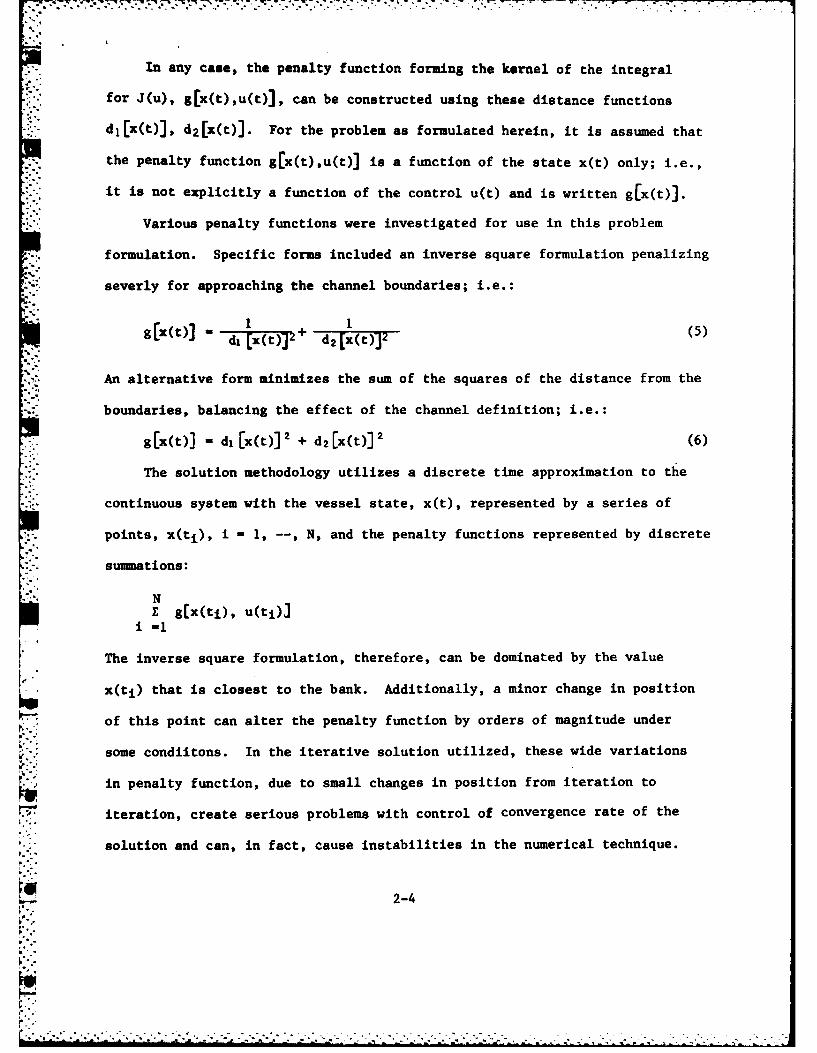
In any case, the penalty function forming the kernel of the integral

for J(u), g[x(t),u(t)], can be constructed using these distance functions

d1 [x(t)], d2 [x(t)]. For the problem as formulated herein, it is assumed that

the penalty function g[x(t),u(t)] is a function of the state x(t) only; i.e.,

it is not explicitly a function of the control u(t) and is written g[x(t)].

Various penalty functions were investigated for use in this problem

formulation. Specific forms included an inverse square formulation penalizing

severly for approaching the channel boundaries; i.e.:

g=t - da +x(t)J+ d2 X(t) 2 (5)

An alternative form minimizes the sum of the squares of the distance from the

boundaries, balancing the effect of the channel definition; i.e.:

g[x(t)J - di [x(t)] 2 + d 2 [x(t) 2 (6)

The solution methodology utilizes a discrete time approximation to the

continuous system with the vessel state, x(t), represented by a series of

- points, x(ti), i - 1, --, N, and the penalty functions represented by discrete

summations:

NE glx(ti), u(ti)A

i -I

The inverse square formulation, therefore, can be dominated by the value

x(ti) that is closest to the bank. Additionally, a minor change in position

of this point can alter the penalty function by orders of magnitude under

some condiitons. In the iterative solution utilized, these wide variations

in penalty function, due to small changes in position from iteration to

- iteration, create serious problems with control of convergence rate of the

solution and can, in fact, cause instabilities in the numerical technique.

F! 2-4

.7

Also, the inverse square formulation requires that the trackline never

cross the channel boundaries, resulting in a problem of properly selecting

the initial trajectory in the iterative process so as to be totally contained

within the channel. Alternatively, complex methodologies for moving channel

$. boundaries to encompass the trajectory and to finally converge to the desired

channel are required. Based on these implementational considerations, and

based on experiments and investigations yielding closely equivalent behaviors

with the quadratic distance from the boundaries penalty function, the latter

was chosen for inclusion in the VNSS.

2.2 General Problem Solution

The general problem as defined above, e.g., find u*(t) to minimize:

J(u) - h[x(tf)] +f g[x(t),u(t)]dt (7)to

with x(t) related to u(t) through:

1(t) = a[x(t),u(t)] (8)

is solved through application of generalized calculus of variations. This

technique introduces a set of functional Lagrange multipliers called co-state

variables or adjoint variables, donated herein by p(t). The adjoint variables

p(t) have the same dimensionality as the state equations x(t); viz., if (as

in VNSS case) there are 6 state variables x(t), there are 6 adjoint variables

p(t).

The calculus of variations formulation then considers an augmented penalty

function called the Hamiltonian which is defined as:

i[x(t),u(t),p(t)] = g[x(t),u(t)] + pT(t){a[x(t),u(t)]4 (9)

2-

-. 2-5

The necessary conditions for a control function u*(t) to yield an optimal

trajectory x*(t) are then:

H*(t) - [x*(t),u*(t),p*(t)(10)

.*(t) --- E[x*(t),u*(t),p*(t)] (11)

-..0 _ Cx*(t),u*(t),p*(t)J (12)

It can be noted that the first set of equations for !*(t) represents an identity

with respect to the state equations of motion, the second set defines the adjoint

variables, and the third represents a gradient stationarity condition.

This set of coupled differential equations have the boundary conditions,

for the fixed final time problem as previously defined, with the initial state

conditions:

x*(to) - x(t o ) (13)

and final adjoint conditions:

p*(tf) h- [x*(tf)] (14)ax

This set of coupled differential equations, with part of the boundary conditions

specified at the initial time and the rest of the boundary conditions specified

at the final time, is referred to as a two-point boundary value problem (TPBVP)

and, with only certain exceptions, is not amenable to analytic solution.

For any specific case, except for the particular exceptions which are

inapplicable to this problem, the TPBVP must be solved using a numerical

technique.

2.3 VNSS Problem Specifics

The general problem formulation and solution defined above will be applied

to the specific problem of vessel navigation within a restrictive waterway. The

system is represented by a 6-state variable set of differential equations. The

2-6

. ° . - . o • . • . -,, .. . .

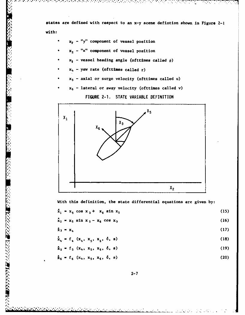
states are defined with respect to an x-y scene defintion shown in Figure 2-1

*1- with:

x* - "y" component of vessel position

* X2 - fox1i component of vessel position

x, - vessel heading angle (ofttimes called 4i)

* X4 - yaw rate (of ttimes called r)

* x5 - axial or surge velocity (ofttimes called u)

x6- lateral or sway velocity (ofttinies called v)

FIGURE 2-1. STATE VARIABLE DEFINITION

X5X,

X6 X3

X2

With this definition, the state differential equations are given by:

ii =x 5 Cos x 3 + x 6 sin x. (15)0X2- xS sin x3 - x6 Cos x3 (16)

i3 = X4 (17)

-=f 4 (x,4 x5, X6, 6, s) (18)

:k f5 (X41 X5, X61 6, a) (19)

A6 f6 (X4, X5 1 X6, 6, 8) (20)

2-7

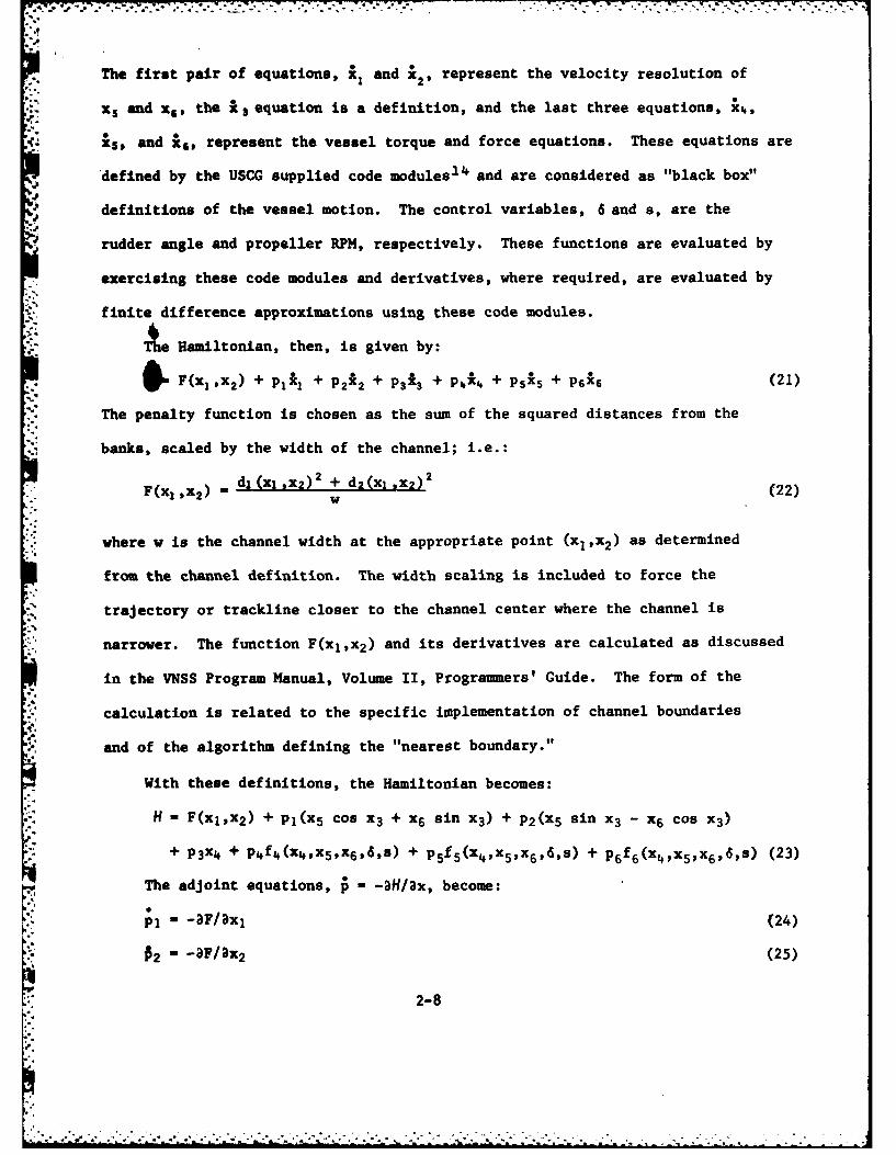
The first pair of equations, 1, and A2i represent the velocity resolution of

x5 and x1, the :13 equation is a definition, and the last three equations, ;4,

xs, and As, represent the vessel torque and force equations. These equations are

J "defined by the USCG supplied code modules1 4 and are considered as "black box"

definitions of the vessel motion. The control variables, 6 and s, are the

rudder angle and propeller RPM, respectively. These functions are evaluated by

exercising these code modules and derivatives, where required, are evaluated by

finite difference approximations using these code modules.

A Hamiltonian, then, is given by:

F (xI ,x2) + pi:1 + P212 + p 3k3 + p4*4 + psIS + P6(6 (21)

The penalty function is chosen as the sum of the squared distances from the

banks, scaled by the width of the channel; i.e.:

SF(x ,x) -d 1 (Xl ,x2) + d2 (xI ,X2) 2

=(II2 w (22)

* where w is the channel width at the appropriate point (XlX2) as determined

from the channel definition. The width scaling is included to force the

trajectory or trackline closer to the channel center where the channel is

narrower. The function F(x1,X2) and its derivatives are calculated as discussed

in the VNSS Program Manual, Volume II, Programmers' Guide. The form of the

calculation is related to the specific implementation of channel boundaries

and of the algorithm defining the "nearest boundary."

With these definitions, the Hamiltonian becomes:

H - F(xl,X 2) + Pl(X 5 cos x3 + x6 sin x 3) + P2(X5 sin x3 - X6 cos X3)

+ p3X4 + P4f4 (x4 9,x5,x6,98,s) + P5f5 (x4,x5,x6,6,s) + P6f6 (x4 ,x5,x6 ,6,s) (23)

U, The adjoint equations, = -aH/3x, become:

-1 -aF/3xl (24)

f2 -F/ax 2 (25)

2-8.4.

. •....- --.°. ..-.- -•-V . . ..

03 -a lX 3 = -P1(X6 cos x3 - x5 sin x3)

-P2(X5 COS x 3 + x6 sin x3) (26)

-H _ -f- af _ af (27)ax4 ' P axL% - P5--ax 4 - ax--f

"" -aH = _ (28)P5 w A - x - px5f - P6 x -P1 cos x3 - P2 sin x 3

- X --~ax5 aX5 ax50 - - a~ _f (29)

p-p62i 0 - - p, sin x3 + P2 cos x 3

aX6 aX6 aDX6 aX6

The final condition is

a- af af- af 0 (30)-.P4 P5_ P636

a6 a6

aH p ag _ f s (31)

as P4S - P5aS - P63s (

The boundary values are the 6 initial conditions:

x*(to) = X(to) (32)

which usually reduce to:

x1 (to) " x (33)

X2 (to) m y. (34)

-" x 3 (to) - 0 (35)

x4 (to) - o (36)

x5 (to) " v (37)

x6 (to ) -o (38)

where the vessel is at some point (X,Y) with heading i, with zero yaw rate,

zero drift angle, and speed v. The boundary values for the adjoint equations

are as defined in the mathematical discussion, with h x(tf) not present in

the object function:

Pi(tf) 0 i 1,6 (39)

2-9

--------I.-. "| " ", --. . . . ". . ". . ".. ., ", . . . . " " '

The solution of this TPBVP with 6 state equations, 6 adjoint equations,

and 2 gradient stationarity conditions then will yield the optimal control

functions 8*(t) and s*(t), and the associated optimal trackline definition.

2.4 Solution Methodology

As previously indicated, the complexity of the f4, f5, and f6 equations

precludes an analytic solution of the above TPBVP for 6 and s*; thus, a

numerical solution methodology is required. The method of steepest descent

has been selected and implemented in the VNSS.

The method of steepest descent, as applied herein, is an iterative

procedure related to the steepest descent or gradient search applied to a

scalar function of several variables.1 5 In this technique, an initial guess to

the solution is selected, indicated by u() (t). While the technique is defined

as a time continuous process, the implementation is with finite step discrete

approximations to the continuous function, with Taylor series integration of the

differential equations defining ; and p.

With this initial guess of control, the state equations (c) are integrated

forward from to to tf yielding the state solution with initial condition x(to).

Then, with the vessel states known, the adjoint equations are integrated

backward from tf to to with "starting" final state p(tf) - 0. Then having

both the states x(t) and adjoint variables p(t), the gradient components

6H/6u can be calculated.

To find a minimum of the objective function J, a step is taken in the

direction of decreasing J or in the negative gradient direction, i.e.:

u(1 (t) u ) t- T6I( ° ) (40)6u

2-10

5,e

n ..h ,-. mm mm .n. .- ' l ,-..,., ,- --, ,, m ,. m . .

%'

% The step T is selected through a single variable search, i.e., T is chosen for

any iteration to minimize the value of the objective function J. The process

is then repeated with control history u( . The method of steepest descent can

be summarized by the following procedure:

1. Select an initial guess u(i ) (t) for iteration i 0

2. With control u (t), integrate the state equations forward with

initial conditions x(to ) to obtain x~1 (t)

3. With this control, u (t) and state x (t), integrate the adjoint

equations backward with final condition p(tf) - 0 to obtain.(:

p I~t)

4. With control u (i ) (t), state x(i ) (t), and adjoints p(i) (t), calculate

the gradient 6H (i)(t)

5. Find T through a search procedure such that:

: u(t) = UMi (t) - T i (t) (41)

a u

minimizes J[u(t)]

6. Let:(i+1 Ml 6H~i (t) (42)

0, .i)(t) = u(1(t) TT6u

7. Go to step 2.

SThis procedure is numerically implemented in the VNSS, with the initial

choice;

8 (o)(t) - 0 (43)

s(o)(t) - initial RPM (44)

The techniques and variables to control the convergence, step size search,

rand number of iterations performed are discussed in the Programmers Manual.

2-11

-- A

2.5 Objective Function in Line Segment Channel

The objective function minimized by the VNSS program is quadratic scaled

by the channel width and summed at each point where the trajectory is evaluated.

A typical point (X,Y) is shown within the channel boundaries in Figure 2-2.

From the geometry of the figure, the objective function for the point is

- dl2 + d22f 2 (45)

w

FIGURE 2-2. OBJECTIVE FUNCTION DEFINITION - TYPICAL POINT

(xp,1p 0 07 (xI+ 1,y1+j) (x1+iyI+i)

( 1jPyyj ) +1W~~x,Y)\

,..-7. "o0u2

A more convenient mathematical representation is the so-called slope/intercept

formulation. This formulation describes a straight line as:

y mx + b (46)

YYI-Ilwhere, m - b - mx1

(In the unlikely event that the denominator of m is sufficiently small as to

cause numerical trouble, an appropriate fix is as follows:

% If lxI -< 10-2, then x, x, + 2.* 10-2

Although this safeguard is included in the code, there is a stipulation in the

Users' Manual which precludes vertical segments.)

2-12

The perpendicular from the line, y = mx + b, to the point (X,Y) intersects

the line at a point (xp, yp) which is given by:

• ""X + m(Y-b) mY + mX + b.-p p b (47),:Xp-P I + M YP 1 + M2

By assumption, the point (X,Y) has already passed the point (xi-l, yI- 1).

Therefore, to determine whether or not it has passed the point (xI, yi), it is

only necessary to check the following:

If Ixp - Xi_ 11 > lxi - xi..l then, it has passed (xj, yi);

otherwise, it has not.*

When it has not passed the point (xi, Yj), then the appropriate penalty

function (for the upper bank) is:

f W (X - xp)' + (Y - yp)' (48)

Substitution of (47) into (48), after simplification, leads to:

(W + b - Y)zf -(1 + m')w (49)

The rate of change of (49), with respect to the vessel position (X,Y)

is given by:

Hf 2m(mX + b - Y) if -2(mx + b - Y)

ax (1 + m')w y ( + m')w (50)

For computer generation purposes, this can be simplified by the sequential

calculation of (49) followed by:

af -2f (51).y (mX + b - Y )

af af (52)

ax ay

In the event that the point (xI , y1 ) has been passed by (X,Y), then

two alternatives arise which are depicted in Figure 2-3.

d *Note: yp need never be calculated.

2-13

, - • - ; ' , : ,, .' . ', '.' ' .- . . , . • . .- . . . . . . ._ . ... . ,

FIGURE 2-3. OBJECTIVE FUNCTION DEFINITION - CORNER POINT

(X1, Y1)

(xI1, , x::-,'1" YI-l) " Xi , Yi l ,. ,Y )

(a) (b)

In order to make the appropriate determination, the procedure is to

first, increment I by 1 and recalculate and store the appropriate m and b

which are given by (46). Secondly, calculate xp with the m and b as given by

(47). Then perform the check:

IF 1xP - xII > jIX 1 - xij, then, Figure 2-3b applies.

Otherwise, Figure 2-3a applies.

In the latter situation, f is computed by (49), and the partial derivatives

/ay and /x are given by (51) and (52). In the situation shown in

Figure 2-3b, that is, when the previous test is passed, then different

calculations need to be implemented.

The appropriate formulas* are:

f (X - x_])* + (Y - Y 1 )2 (53)

af a(X - x1 . 1) (54)ax

af a(Y - YI-1 )• " " w(55)

*Note: The subscripts referral in (53), (54), and (55) pertain to theincremented subscripts in Figure 2-3.

2-14

4' " , ""ia m -" - m i m m ' m m . .d "

3. SIMULATION CAPABILITIES AND LIMITATIONS

3.1 Simulation Capabilities

The optimal control techniques for determining a vessel control history

and resultant trackline, as defined in the previous section, have been embedded

in the Vessel Navigation System Simulation (VNSS), delivered and installed on

the USCG PDP-11/34 computer system. The detailed discussion of the program

structure, particular algorithmic formulation of certain design features, and

input/output formats is relegated to the VNSS Program Documentation, Volume I,

Users' Manual and Volume II, Programmers' Manual; the overall VNSS capabilities,

features and limitations will be discussed herein.

The VNSS is constructed to accept definition of a scenario consisting of

an arbitrary (within limits to be discussed) channel definition including

obstacles, current and limited pilot visibility or field-of-view, along with

a detailed vessel definition, and to construct the control history and resultant

- trackline, using the technique previously described. Two primary goals

were observed during the derivation and construction of the algorithms and

simulation; firstly, the scenario definition should be as general as possible

or practical and, secondly, the formulation and solution of the optimal control

.4.-

problem should be transparent to the user. In addition, a convenient form

I Bof user input for maximal utility and flexability was considered as mandatory.

*' Design trades between global scenario generality and computer program design

considerations including problem execution time yielded the final form of the

:simulation specifications discussed herein.

The major problem scenario definition elements of the VNSS are indicated

in Table 3-1 and discussed in detail below.

3-1

°= . . ." . . . . . . . . . . . .

TABLE 3-1. SCENARIO DEFINITION ELEMENTS

Vessel Definition (Dynamics)

Channel Definition

Current Definition

Obstacle Inclusion

Scene Analysis

The VNSS is constructed based on the vessel and dynamics as defined by

the USCG supplied "black box" code. Within this code, the vessel is defined by

a set of hydrodynamic coefficients residing in the "DTM10" subroutine. The

VNSS is therefore based on the same set of coefficients and requires linking

of the proper "DTNL0" subroutine through the taskbuild process. This vessel

definition is the only mechanism provided, no alternative vessel definition

process is incorporated.

Similarly, the only vessel dynamics is through the USCG supplied

subroutines "FWL0", "CURT", "DRV10", and "DRUl0". These subroutines derive the

forces and moments due to vessel hydrodynamic interaction, winds, currents,

rudder application, and propeller RPM. These forces are then converted to

accelerations in the state variables, accounting for the fact the x5(u) and

x6(v) are in a rotating coordinate system with rotation rate xN(r). These

accelerations are then integrated using a Taylor series type of integration.

These USCG supplied subroutines have been included in the VNSS with no

alterations in the operational code sequence. Additionally, these subroutines

are used in a finite difference approximation for the various derivatives of

accelerations (f4 , f5, and f6 of Section 2) with respect to the respective

variables (x4 , X5, x6, 6, and s of Section 2). Again, no alternatives or

options to this definition of the vessel dynamics is provided.

'4 j-2

The channel definition is patterned after and is compatible with the

channel specification procedure in the USCG supplied subroutines. This

compatibility was enforced to allow use of the channel scenario as defined

- through the "DTN1O" subroutine as a default option. Again, the proper "DTN10"

subroutine corresponding to a particular predefined channel must be linked at

taskbuild. In addition, capability is included to create a new channel

definition, modify the default (DTNIO) option, or modify a predefined channel

definition. Implementation and execution of these options is discussed in

the VNSS Program Documents.

The channel is defined by a series of straight line segments, or "splines,"

with the segments specified by the coordinates of the breakpoints of the

splines. The breakpoints must be specified in pairs, with one on each bank.

This requirement is necessary to enforce compatibility with the USCG supplied

"CURT" and the ,"DTN10" options. The intent of the breakpoint is to t ughly-

span the channel, with minor variations being non-catastrophic in .ature.

To again enforce compatibility with the USCG supplied "CURT" subroutine, a

maximum of 30 breakpoints are allowed.

The current is defined by specifying the current speed and heading at

eight stations across the channel, at each pair of breakpoints. These stations

are equally spaced at positions (2i+l)/16 i f 0,7 along the line joining

*' the pair of breakpoints. This definition is again consistant with the USCG

supplied subroutine "CURT" which interrogates the scene to find the current

value at any (X,Y) point by associating the point with the geometrically

closest current definition point. This algorithm defined by "CURT", while less

accurate than a true interpolation scheme, was adopted through the use

of "CURT" due to the interface structure already defined between "CURT" and the

other USCG supplied subroutines. Again, the default values of current are

3-3

.. "."".7

input through the linking of a proper "DTNLO" subroutine. Also, options to

input a new current definition related to a new scene, or to alter the current

definition in the default or in an existing scenario are included.

*-"- Finally, the current can be deactivated; i.e., all current values are

*ignored (equivalently zero) by setting a single switch. This option, by

eliminating all calls to subroutine "CURT", can reduce program run time by

up to 2/3 as the program spends 1/2 to 2/3 of the execution time in "CURT"

when it is activated, as established through timing experiments with the

code.

The VNSS can include up to five discrete obstacles in the channel. Each

* "obstacle is specified by a position (X,Y) and by an indication as to with which

bank the obstacle is associated. This association forces the trackline to pass

between the obstacle and the opposite bank; logic for automatically selecting

-the best bank association for a given obstacle is not currently included. The

obstacles are included in the internal optimal control problem solution only

when they occur within the pilots field-of-view, i.e., are within the specified

visibility range or "window" from the current vessel position.

The VNSS is designed to simulate a limited field-of-view or visibility

range for a pilot. From any given point, only those bank segments and obstacles

within this field-of-view are included in the internal objective function

calculation and thus affect the solution. This limited field-of-view is

referred to as a "window" and the solution proceeds along the channel using a

* so-called "sliding window" solution.

Z-, The beL.. solution nethodology would therefore be to calculate the optimal

control and trackline for the next window and use this control to advance one

* time step (nominally hard-coded as 2 seconds). At this new position, a new

window is defined, the problem again solved for this new window, slightly

3-4

offset down-trajectory from the previous window, hence the term "sliding

window." In a practical environment, the execution time of this solution

methodology is quite excessive with the optimal control problem resolved at

each and every time point. Thus, the implemented solution is to specify a

restart position at which a new window is constructed as an approximation to

the continuous sliding window. The observation window length and restart

length are specified independently; experiments performed by Delta Research,

Inc., indicate, however, that restart lengths approximately 1/3 of a window

length, i.e., the next window overlaps the previous window by 2/3, represent

a good compromise between trackline performance and execution time. Additionally,

if the restart length is equal to the window length, and both are equivalent to

the scene length (also user specified) the resultant trackline is generated in

one single window with all down-trajectory information available to formulate

the solution. The scene analysis is then controlled by three variables, viz.,

the window length, the restart length, and the overall scene length.

* 3.2 Simulation Restrictions

During the construction of the VNSS, the goal of total generality of the

scene definition was tempered with the objective of keeping simulation run time

* minimal. This trade results in algorithms for calculating the nearest bank

segment, the appropriate objective functions, and the derivatives of the

objective function that place minor restrictions on the global generality of

the channel definitions and on the relationship of the obstacles with respect

4 to the bank spline breakpoints.

The primary restriction is with respect to the angular relationship between

adjacent splines in the channel definition as sharp bends between adjacent

4 splines, particularly convex bends where the bank bends into the channel, can

have a deleterious effect on the algorithm that calculates the objective

3-5

function and its derivatives. This restriction can be quantified as no more

than a 350 bend between adjacent spline segments. Thusly, for example, a

right angle bend in the channel should be modelled as three breakpoints with

350 between splines. The 35' limit is not a "hard" limit, as there is no

catastrophic program failure at, for example, 360 between splines. However,

as the angle increases beyond 350, the probability of anomolous simulation

behavior increases.

The breakpoints to define the splines must be sequential in the direction

of vessel travel with convention that the scene be roughly horizontal with the

vessel travelling from left to right. This restriction is generated by the

need to keep the subroutine that establishes the vessel location in the channel

simple, to avoid the execution time overhead imposed by an algorithm such as

"CURT". Additionally, spline segments should be a minimum of 300 feet in length

and in no case can a spline segment be vertical. Since channel width is

determined by the geometric distance between a pair of breakpoints, the break-

points should nominally span the channel.

The obstacle definition is by location and association with a particular

channel boundary. As such, the location must be a point within the nominal

channel to avoid catastrophic program breakage. The VNSS incorporates the

obstacle into the appropriate channel boundary by moving the adjacent spline

breakpoints such that the appropriate bank segment passes through the obstacle.

Following this, the spline breakpoints further from the obstacle are altered

to maintain the maximum angular change between adjacent splines as discussed

previously. In order to accomplish this, there must be breakpoints "near"

the obstacle to allow the algorithms maximum flexibility in fairing the

obstacle into the bank. While general in nature, the algorithm as implemented

in the VNSS cannot anticipate every potentially possible combination of

3-6

.. I - - . - -. . - .- ---. . .. .. - - - -- " • . - . -, • • - - . • " .

*i obstacles and breakpoints. Thus, a general set of rules for defining

auxiliary or artificial breakpoints "near" an obstacle are given. Since

under some particular circumstances, the obstacle fairing can adversly affect

the channel definition, the channel as redefined with the obstacle faired in

is output to the user to allow examination and modification of the artificial

breakpoints if required. Every attempt has been made to keep the algorithm

robust within the general set of rules below, although the user can always

find a particular input to break the algorithms.

The artificial breakpoints must, of course, be specified in pairs across

the channel. The artificial break points should be closely spaced, at about

the 300 feet minimum, and there should be several pairs of points on each side

* . of the obstacle. Since obstacles extending well within the channel require a

greater fairing, three pairs of breakpoints on each side should be specified.

For obstacles near the bank, two pairs on each side of the obstacle should

suffice. Finally, for obstacles in a general curve in the channel, the break

points should fill in the curve and also extend around the curve into the

straight segments, if required, to get the requisite to two or three artificial

pairs. Alternatively, the user can himself fair the obstacles into the banks

- . and enter the resultant modified channel definition as if it contained no

obstacles. The user can also "failsafe" the problem by specifying the entire

channel in 300 foot segments. The VNSS should be robust to problem specifications

within the above conventions and restrictions.

The scene is specified through the window length, restart or "slide" length,

and total scene length. Certain "rationality" conditions must be met, e.g.,

the scenario length must not exceed the channel specifications and the restart

length must be within the window length. The total scenario length is limited

to 500 time steps, nominally chosen at 2 seconds for 1,000 seconds of travel. For

3-7

a typical tow flotilla with velocity in the order of 10 ft/sec, this allows

about 10,000 feet of scene definition. Finally, the distance specifications

must not be "microscopic" with respect to the problem definition, i.e.,

distance specifications should be at least in the order of hundreds of feet.

The final comments are with respect to the convergence of the solution.

As discussed in Section 2, the optimal control problem results in an iterative

solution of the TPBVP. The "quality" of the solution found by the steepest

descent method increases with increasing iterations at the expense of computer

execution time, although the adaptive step size algorithm implemented tends -to

mitigate this to some degree. The stopping criterion is automated, although to

a rudimentary degree. The iteration stopping criterion is user specified as a

number of "fine tuning" iterations after the first iteration that yields a

* trajectory totally within the channel specifications. There is an automatic

override of this stopping criterion if the iterative procedure is still in a

* rapidly converging situation, which allows further iterations until the

* convergence rate slows or a maximum of twice the specified number of fine

tuning iterations occurs. Additionally, there are automatic limiting

criteria in the adaptive step size algorithm.

It is axiomatic to the mathematical formulation of the problem that

short, simple scenes converge faster than long, complex scenes containing

reverse ("S") curves; therefore, execution time considerations favor "sliding

window" solutions for long, complex scenarios rather than single pass solutions.

Experiments have demonstrated that under relatively general conditions, the

control histories generated by the two problem specifications (sliding window

versus single pass) are closely aligned with virtually identical tracklines

generated.

3-8

i; '. - -; . - - ': ' " ,'* . '. ' -' - ."

" . . - ---. - - , . -' : ; -. : . ": - ., . -: , .- - . ;- . " , -- -

4. NUMERICAL EXAMPLES

The VNSS as delivered to the USCG has been exercised on sample scenarios.

These scenarios all utilized the USCG supplied model of the Exxon Tennessee

towboat floatilla. This model is defined, as discussed previously, by the

USCG "DTM1O" subroutine in terms of physical parameters and hydronamic

coefficients. The towboat floatilla is roughly 745 feet long by 54 feet wide.

In all cases, a maximum rudder command limit of .7 radians (40.10) is observed:

also, the vessel nominal (zero drift angle) steady state velocity is roughly

10 ft/sec at 100 RPM. The examples examined include an arbitrary "S" turn

channel, an arbitrary channel with a more gentle turn, a segment of the

Mississippi River (Berwick Bay), and a problem defined to indicate vessel

response in a simple scenario.

The response of the towboat floatilla is very sluggish, requiring the

anticipatory nature of the solution as previously discussed. The characteristic

response is shown in Figure 4-1, which shows the vessel response to a 300

rudder command, at initial velocity of 10 ft/sec at 100 RPM. The vessel is

headed due east, along the "X" axis, when the rudder is applied at (0,0).

The distance to achieve various lateral offsets are shown in Table 4-1.

TABLE 4-1. LATERAL OFFSET DISTANCES

TIME (SEC DISTANCE (FT) LATERAL OFFSET (FT)

0 0 038 365 -858 531 095 920 100

115 1080 200

The initial motion is due to the force on the rudder before a drift angle is

achieved, and is 8 feet to the left for the right rudder case shown. It

requires 531 feet to compensate for this and achieve zero offset, with theI

offset then increasing ever more rapidly. The final steady state turn radius

is 690 feet.

4-1".,

FIGURE 4-1. EXXON TENNESSEE RESPONSE

0

-200

-400

-600

:i::! -800-8 300 RUDDER

100 RPM

-000

-1200

-1400

0 200 400 600 800 1000 1200 1400X DIRECTION - FT

Example 1

This example consisted of a channel defined by 16 pairs of spline break

points, indicated in Table 4-2 below.

TABLE 4-2. SPLINE BREAKPOINTS

"Lower" Bank "Upper" BankX Y X Y

800. 2200. 800. 3200.1600. 1400. 1600. 2400.2000. 1000. 2400. 1600.2700. 750. 2700. 1500.3000. 600. 3000. 1400.3300. 700. 3300. 1500.3600. 800. 3600. 1600.3900. 900. 3900. 1900.4200. 1000. 4100. 2100.4400. 1200. 4300. 2300.4600. 1400. 4600. 2400.5000. 1500. 5000. 2400.5400. 1400. 5400. 2300.6000. 800. 6000. 2200.6400. 500. 6400. 2000.6800. 200. 7000. 1400.

4-2

There are two defined obstacles as shown in Table 4-3.

TABLE 4-3. OBSTACLE DEFINITION

Position (X,Y) Bank Association

(2900., 1200.) Upper

(4000., 1200.) Lower

Figure 4-2 shows the channel definition. The points indicated with circles

were added as "auxiliary" points for purposes of fairing in the obstacles, also

indicated.

FIGURE 4-2. ORIGINAL CHANNEL

4

U-'3

C-,

1 2 3 4 5 6 7 8

X DISTANCE - KFT

Figure 4-3 indicates the channel as defined with the obstacles faired into

the bank definition. The use of the auxiliary spline breakpoints is clearly

indicated in the figure. In addition, the lower corner at (3000, 600) has

also been "smoothed" to conform to the maximum segment-to-segment bending

criteria.

4-3

FIGURE 4-3. AUGMENTED CHANNEL

4 -

I i 3-

.': 2 "im

0

1.

1 23 4 5 678

X DISTANCE - KFT

The initial vessel position is parallel to the right bank at the location

(1400., 1700.). The vessel's initial speed is 10. ft/sec with RPM setting of

150 RPM.

The resultant trackline for a full passage of the channel in one window

is shown in Figure 4-4 after 50 iterations.

FIGURE 4-4. TRACKLINE-LONG WINDOW

4-

-4-

*'o . I ,I

0" .. 1 2 3 4 5 6 7 8;J X DISTANCE - KFT

i 4 .",.-4-4

The scenario was also executed with a sliding window of 3000 feet, with restart

after 1000 feet. The convergence criteria was set to five fine tuning iterations.

This trackline is shown overlaid on the previous in Figure 4-5. Differences

are attributed to the use of only 5 fine tuning iterations; 10 or even 20 is

preferable.

FIGURE 4-5. TRACKLINE-SLIDING WINDOW

* 4-

3-I-.

-

C,);.... ..

I I.I I I"

0 1 2 3 4 5 6 7 8

X DISTANCE - KFT

The rudder control functions are shown in Figure 4-6. Both cases show

the hard transition from left rudder to right rudder at the switchback point,

just past the apex of the left bend. The sliding window case would probably

have maintained more left rudder in the initial portion with more fine tuning

iterations. Also, the jump in rudder between the second and third window is

characteristic of the form of solution, as the sliding window reinitialization

does not enforce mathematical continuity of solution.

4-5

FIGURE 4-6. RUDDER HISTORY

.6

LONG WINDOW

.4j.,.2

L WSLIDING WINDOW

* /

' X DISTANCE - KFT

.4 -c

.6

In addition, the rudder control must always go to zero at the .end of the

scene due to the inherent formulation of the problem as implemented in the

VNSS. Alternative formulations could enforce other rudder or vessel terminal

conditions.

This example demonstrates the basic simulation capabilities, including

channel definition, obstacle inclusion, and limited observation (sliding

window) mode of operation.

Example 2

This scenario consists of a channel with 15 brea.k, ints, shown in Table 4-3.

4-6

TABLE 4-4. SPLINE BREAK POINTS

"Lower" Bank "Upper" Banki x Y

400. -400. 0. 0.1000. 200. 600. 600.1500. 700. 1200. 1200.1800. 1000. 1800. 1800.2100. 1100. 2100. 1900.2500. 1000. 2600. 1800.2750. 750. 2750. 1650.2900. 600. 3000. 1400.3250. 250. 3300. 1100.3700. -200. 4000. 300.4000. -500. 4300. 0.4500. -1000. 4500. -200.5200. -1300. 5600. -700.6200. -1300. 6200. -700.9000. -1300. 9000. -700.

Three obstacles are included, defined in Table 4-5.

TABLE 4-5. OBSTACLE DEFINITION

Position (XY) Bank Association

(2800, 1400) Upper(3900, -300) Lower(6000, -800) Upper

Figures 4-7 and 4-8 show the channel, obstacles, and resultant "faired"

banks. The points shown with circles are auxiliary spline breakpoints defined

for obstacle smoothing.

FIGURE 4-7. ORIGINAL CHANNEL

2

°.1- X - KFT

""2 3 7 8 9

-2

4-7

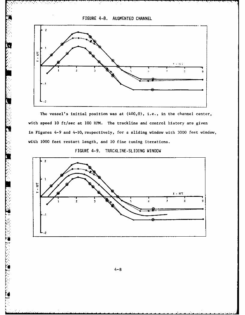
FIGURE 4-8. AUGMENTED CHANNEL

•. -.. •... •s •. --o o - - o

......... .

The vessel's initial position was at (400,0), i.e., in the channel center,

- with speed 10 ft/sec at 100 RPM. The trackline and control history are given

in Figures 4-9 and 4-10, respectively, for a sliding window with 3000 feet window,

* with 1000 feet restart length, and 10 fine tuning iterations.

FIGURE 4-9. TRACKLINE-SLIDING WINDOW

W ..... .......................... ...,-2

6- 4-8

d,

With the rudder angle 6 in radians and the propeller shaft speed in RPM, these

(for a given point in the trajectory) have values shown in Table 4-6.

TABLE 4-6. DERIVATIVE VALUES

Adjoint Partial Derivatives

P4 =3. X 105 4 'X4 1 - 5 10-3a RPM .4 X 10 .5 X

p 5 3. x1 3 = .710 xO 3 Xa= l xlO -.7 X1036 "

P6= .7 X 102 .=5 X 10-_ = 5 X 10aRPM = X6 1

aH = 2.2 ft/RP aH_ 184 ft/rada RPM ftRP

The difference in the gradient values of two orders of magnitude results

• :in the solution to converge strongly in the rudder direction without significant

alchange in RPM. Theoretically, as approaches zero, the RPM will converge.

• . However, the two order of magnitude difference precludes this from occurring

in the numerical method utilized. This scaling was investigated by artificially

multiplying the RPM gradient by a constant value or, equivalently, treating

T as a matrix rather than a scalar. Table 4-7 shows the results of these

. experiments.

TABLE 4-7. RPM SCALING

Scaling Factor Initial RPM Final Objective Function

50 99 38315100 98 38248200 * 97 38493500 80 37427

1000 85 376035000 50 36272

The RPM, in all cases, increased smoothly from the initial value to 100 RPM

final value, as dictated by the mathematics. The primary reason for the decrease

*| 4-10

I

FIGURE 4-10. RUDDER HISTORY

.6

- .3

.2

-.3

-.4

Once again, the discrete jump in rudder command at window restart is indicated,

The vessel servomechanism response delay time, limiting rudder swing to 5 deg/sec

would damp this discrete jump. This servomechanism response delay is high

bandwidth with respect to the vessel response time and, thusly, is not modeled

in the VNSS as it has inperceptible effect on the resultant trackline.

A detailed investigation was performed with regard to the change in RPM

corresponding to the optimal solution. The RPM is changed along with the

rudder command, with the changes as shown in Section 2 to be:

ARPM T 3H A6 =-T L6R P RPM 9)

These become, as shown in Section 3:

-' aH +__s _ + a _. 6.aR_.RPM 4 PRPM P RPM P PRPM (2)

i a+H6 =P + P5XS + P63 4-S (3)

4-9

in the objective function is the shortening of the trajectory placing more

emphasis in the narrow part of the channel where the objective function is

naturally lower. This cross-coupling between length of trajectory and

objective function makes RPM scaling difficult to generalize, and Delta

Research, Inc., recommends utilizing the unscaled gradient as currently

* implemented in the VNSS.

Example 3

This example demonstrated the response of the algorithm to a simplistic

case. The vessel starts near to the bank in a long, straight channel. The

channel is defined to be 600 feet wide and 5000 feet long. The break points

are as shown in Table 4-8.

TABLE 4-8. SPLINE BREAKPOINTS

LOWER BANK (XY UPPER BANK ,YL

(010) (0,600.)

(5000. ,0) (5000. ,600.)

The vessel starting condition is (50.,50,), i.e., 50 feet off the starboard

bank. There are no obstacles, and the solution was generated in one pass.

Initial velocity and RPM were 10 ft/sec and 100 RPM. Figure 4-11 shows the

trajectories after 5, 11, and 100 iterations, although the trajectory is

stationary aferoughly, 30 iterations.

4-11

FIGURE 4-11. TRAJECTORIES

5 ITERATIONS

11 ITERATIONS

100 ITERATIONS

DIRECTION OF TRAVEL

0 2 3 4 5

(KFT)

The control histories are shown in Figure 4-12.

FIGURE 4-12. CONTROL HISTORIES

RIGHT LIMIT'

5POSITION (KFT)

POSITION (KFT)

i-LEFT LIM1ITJ

0 1 2 3 4 5RIGH LIMT.]11 ITERATIONS

POSITION (KFT)" LEFT LIMITV

' 0 1 2 3 4 5

RIGHT LIMIT l' TRAIN

~POSITION (KFT)

LEFT LIMITL

4-12

E..-,.. ... ,.. ..-. ... . . .. I .

The solution converges to a hard (max rudder limited) turn off of the bank,

followed by a "damping" process to minimize overshoot of the channel center.

The vessel response can be noted to display an initial motion toward the

right bank, to about 42 feet, due to the initial left rudder before a

significant drift angle can be set.

Example 4

This example corresponds to the passage of the Berwick Bay section of the

Mississippi River. It is the scene defined by the USCG supplied "DM10"

subroutine with the current suppressed. The basic channel is shown in

Figure 4-13.

FIGURE 4-13. BERWICK BAY DEFINITION

The two railroad bridges are modelled by fairing the channel banks to

include the bridges. This was done in this case by using the option to create

and input new spline breakpoints to define the augmented channel. The solution

shown is without current and corresponds to 10 ft/sec, 100 RPM initial

condition. The solution is shown in Figure 4-14 with rudder history shown in

Figure 4-15.

4-13

I"p.'

FIGURE 4-14. BERWICK BAY PASSAGE

8

1C"O' RL AM

6

IA~ 4

24 6 8 0 12 14 16

KFT

FIGURE 4-15. RUDDER COMMAND

S.3'

S.2.

2K 4K ;K 8K 10K 12K 14 16K 18K

S.2.

The rudder command for this case peaks at .3 rad or, roughly, 200 rudder

for the initial turn, followed by .22 rad for the reverse turn through the

bridges.

4-14

5. FUTURE ACTIVITIES

Delta Research, Inc., believes that the application of optimal control

theory as a tool for vessel navigation and control studies is a powerful

technique and is applicable over a wide variety of problems and analyses.

This section will discuss, out of these general applications, only those

obvious extensions and applications of the currently developed VNSS. These

extensions and applications fall in the three categories shown in Table 5-1,

viz., efficiency enhancement of the current VNSS, validation of the current

VNSS, and potential extensions of the VNSS capabilities

TABLE 5-1. FUTURE ACTIVITIES

VNSS EFFICIENCY ENHANCEMENT- Run Time Reduction- Scene Capability

VNSS VALIDATION- Validation Plan- Tuning

"-VNSS UTILIZATION AND EXTENSIONS- Capability Extension- Sensitivity Studies

5.1 VNSS Efficiency Enhancement

The VNSS, as currently configured, executes on the USCG PDP-11/34 slower

than real time with the actual ratio dependent on scenario. Reduction of this

run time would enhance the utility of the simulation for some applications. A

primary technique for execution time is through accelerated convergence

techniques. The gradient search technique is a basic numerical technique used

for this class of TPBVP solutions and is generally characterized by slow

convergence. Alternative convergence techniques such as PARTAN16 offer

quadratic convergence, in that the process will find the precise maximum of a

5-1

Ve

quadratic function on the third iteration. Although the objective function is

significantly more convoluted than quadratic (in function space) as inferred

through detail analysis of the converging solution for a sample problem, there

is still great promise for this or other convergence acceleration schemes.

An alternative source of run time reduction is through the use of simpler

dynamics than implemented in the USCG supplied subroutines. This trade of

"* execution time for vessel dynamic model fidelity must, of course, be made based

on the ultimate utility of the VNSS. As an intermediate step in the VNSS

development sequence, Delta Research, Inc., utilized the so-called Nomoto

equations for vessel dynamics simulation. These equations, involving significantly

fewer terms in the Taylor series expansion for accelerations, offer a potential

sevenfold reduction in run time. Finally, for scenarios including current

specification, significant run time reduction can be accrued by simplifying and

streamlining the USCG supplied "CURT" subroutine for interpolating current value

* for a given point in the channel.

The scene is currently limited to 500 time steps or, roughly, 10,000 feet

total length. This limit is imposed by the amount of core available for

variable storage. This can be increased through enhanced use of dynamic

* memo;, or, for a sliding window case, by accumulating the control input only

in large scale memory and recreating the trackline through a post-processor.

This would allow virtually unlimited sliding window problems to be executed.

Finally, the use of direct memory can be enhanced through general array

overwriting when appropriate, i.e., destroying an array as it is used and

utilizing the released memory for storing alternate arrays. These are pure

programming issues rather than fundamental mathematical developments.

I

5.2 VNSS Validation

The test results detailed in Section 4 present the capabilities of the

VNSS and indicate the nature of the solution form. The general control

histories and resultant tracklines are, in the large, representative of

the class of results expected. In this sense, the VNSS model has undergone

some degree of "tuning" to give generally acceptable results. The level of

acceptability, however, is based on a qualitative examination of the trajectory

rather than a quantitative evaluation of the problem solution. This

quantitative evaluation of the VNSS solution methodology is referred to as

the model validation.

The validation of the model for a complex, human interactive process,

such as the closed loop vessel navigation and control process, is generally

by comparison of the model results with the real world implementation of

the process. The real world implementation of the process, however, for the

case in hand, represents passage of a vessel through a complex channel. The

problem with obtaining this reJ1 world implementation is therefore twofold,

e.g., it does not exist for arbitrary channel definition, and controlled

experiments with real vessels in existing channels are prohibitively expensive.

Another potential source of data is observation and data collection on

routine passages of commercial vessels. The detailed data requirements for

full validation, i.e., numerical comparison of model trajectory with the

real vessel trajectory are listed in Table 5-2.

5-3

1:.

TABLE 5-2. VALIDATION DATA REQUIREMENTS

* iSCENARIO DATA. - Channel Definition

- Local Obstacles- Vessel Definition

* ENVIRONMENT DATA- Current Definition in Channel- Wind History

* CONTROL DATA- Rudder Command History- RPM Command History

* TRACKLINE DATA- Position History- Yaw and Yaw Rate History- Speed History

Data collection of lesser fidelity has already been undertaken by the

USCG. 17 Acquisition of the data elements above, with the necessary fidelity,

represents a significant undertaking in all data elements.

The scenario data is the most readily obtainable from charts, visual

observations, and photographic data. However, the vessel must either be

one for which a representation exists in terms of parameters in the USCG

supplied vessel dynamics model, or the vessel dynamic parameters must be

derived and validated. Additionally, the environmental data, current and

winds, must be available or derivable in a form compatible with the vessel

dynamic model, to the degree of accuracy required to support the quantitative

validation. The control data and trackline data must be recorded with time,

granularity, and accuracy commensurate with the quantitative validation goals.

Full utilization of this data will require a mechanical data gathering device,

particularly to obtain vessel absolute position within the channel to a

. 5-4

valid degree of accuracy. This position can be established accurately by

such means as LORAN, NAVSTAR, conventional range and bearing observations,

- triangulated bearings, or aerial photography.

Based on the above discussion, the collection of a comprehensive data

base of detailed quantitative data to allow point-by-point comparison of model

results with real vessel passage appears prohibitively expensive. There is,

however, a possibility of obtaining data on a limited number of passages of

previously modeled vessels in previously modeled channels with known current/

wind characteristics. While this data is extremely useful for validation and

tuning of the VNSS for these particular cases, it does not generally allow

the validation of the model against a wider class of vessel/scenario combi-

nations. Similar analysis concludes that the use of a scale model basin,

such as the CAORF, David Taylor Basin, or Netherlands Model Basin, are

prohibitively expensive except as sources of data on limited vessel/scenario

combinations. Therefore, detailed data from real passages or simulated basin

passages is of cost-effective utility for point-by-point quantitative model

validation, if it can be obtained either "piggy-back" on existing experiments

-' or by inexpensive on-board observations and measurements. Such data is most

useful in the final phases of the validation process, for model certification

after the model is fine tuned through the validation process.

With the unavailability of the above detailed, accurate data at non-

prohibitive expense, the VNSS validation must rely on a process other than

point-by-point comparison of the problem solution to a real passage either

in a channel or in a model basin.

An alternate source of trackline data for comparison purposes is the

USCG man-in-the-loop hybrid "Towboat Maneuvering Simulator," 18 which can be

5-5

utilized to generate a valid passage, or set of allowable passages, of a given

channel with a specific vessel. This facility is extremely cost-effective to

generate realistic passages in a short time. The "quality" of the passage

is, of course, a function of the person exercising the control panel of the

simulation. Therefore, trackline data for comparative analysis must be

generated by a knowledgeable non-pilot or by an expert pilot. Validation of

" the results of the hybrid simulator, to be used as a reference for VNSS

validation, therefore, becomes an issue. However, even with validation of the

hybrid simulation results required, it remains a more viable source of

tracklines and control histories than real or model vessel passages.

Alternatively, validation can be performed through the use of an expert

pilot, to both define a range of realistic tracklines for given problem

scenarios and to review the resultant VNSS control history and trackline

for adequacy as response to the problem scenario. This may include the use of

the hybrid simulator as discussed above. This source of data and evaluation

is extremely cost effective for both model tuning and absolute validation. As

a caveat, however, such validation is a good-bad objective indicator rather

than a detailed quantitative evaluation of the quality of the solution.

-. Additionally, subjective biases may enter the pilots judgement when transferred

from a real vessel scenario to a conceptual problem, i.e., replacing "seat

of the pants" navigation with "intellectualizing" of the problem.

Finally, quantification of solution effectiveness in model validation can

be accomplished through the construction of a figure of merit (FOM) as a

quantitative representation of the attributes of the solution. The important

components of the FOM may be identified with the aid of expert pilots,

experts in pilot behavioral studies, and USCG and other maritime agencies.

5-6

. . .

Components of this FOM may include attribures of the trackline, such as

minimum and average distances from channel banks and obstacles, as well as

characteristics of the control history such as average or total integrated

control utilization, and minimum or average reserve control authority where

reserve control authority is the difference between the maximum achievable

control effort (rudder deflection) and the actual, applied control effort.

:- This latter element has been suggested as one of the considerations of

pilot behavioral analysis. The FOM, as a quantification of the solution

quality, must be derived and developed from the qualitative judgments of

solution quality as discussed above. Once a valid FOM is derived, the

VNSS can be validated against a broad spectrum of scenario and vessel

characteristics quickly, inexpensively, and effectively.

Table 5-3 summarizes the various validation techniques discussed above.

TABLE 5-3. VALIDATION TECHNIQUE SUMMARY

DATA REFERENCE SOURCE COST/EFFECTIVENESS

• Experimental Real Passage Very Poor

- • Model Basin Passage Very Poor

• Fully Instrumented Real Passage Poor

• "Piggy-Back Data Gathering Passage Good for Isolated Cases

- Towboat Maneuver Simulation (TMS) Very Goodand/or Expert Consultation

*-Figure of Merit Analysis Very Good

From the above validation techniques, the last three are most applicable

to the validation of the VNSS. The validation process would start with an

in-depth simulation exercise, where an extensive series of VNSS scenarios would

be constructed, the cost and tracklines generated, and the solutions analyzed

in detail. Expert pilot consultation and, potentially, the TMS as an adjunct

to the expert analysis, would be utilized to subjectively evaluate the

5-7

the solutions and to "tune" the VNSS in terms of the obstacle modeling, channel

boundary effects, and objective functions. Such "tuning" considerations

may include obstacle buffer zones, switching obstacles out of the scenario

under appropriate conditions, and inclusion of the bow and stern or the vessel

corner points in the objective function rather than the vessel center of

gravity as currently modeled.

Based on these experiments, tuning and evaluation, a figure of merit (FOM),

would be constructed and validation would proceed with expert consultation,

the TMS, and FOM anlaysis. When simulation has been extensively validated

through this experimental program of VNSS simulation exercise, and is in a

final state of refinement, a limited series of observed passage data collection

would be performed on an as available, commercial, "piggy-back" basis. VNSS

models of the same passage, bracketing the passage conditions in terms of

the variable (current and wind) elements of the scenario, would be extensively

analyzed and compared to the observed passage data as a final certification of

the VNSS. The schedule for this Validation Plan, spanning 1 years, is

shown in Figure 5-1.

5-8

e

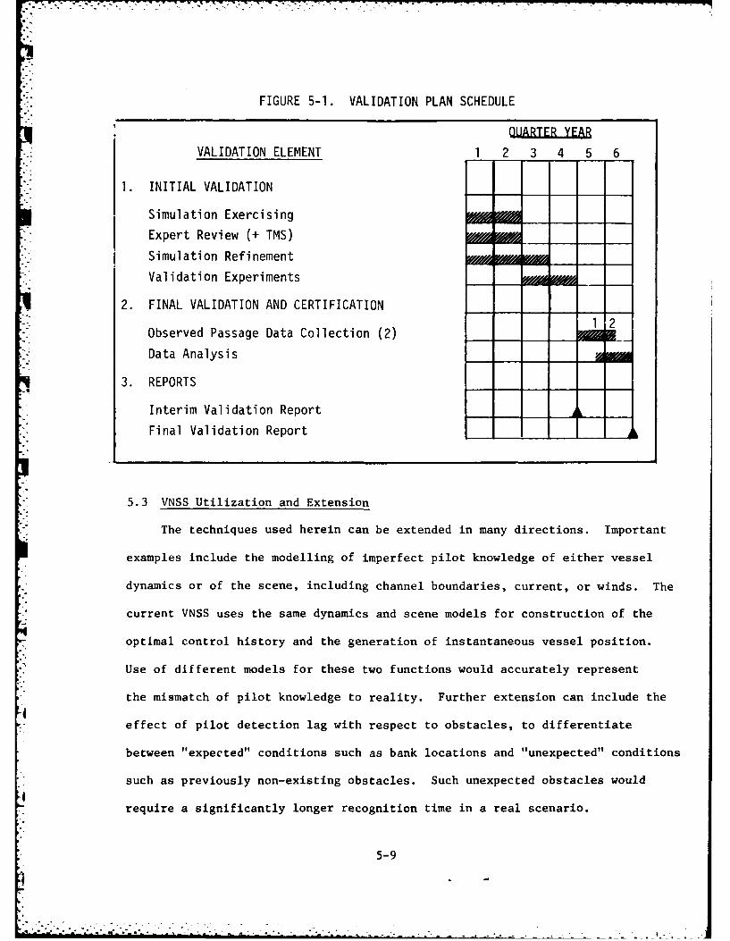
FIGURE 5-1. VALIDATION PLAN SCHEDULE

QUATE YAD

VALIDATION ELEMENT 1 2 3 4 5 6

1. INITIAL VALIDATION

Simulation Exercising

Expert Review (+ TMS)

Simulation Refinement

Validation Experiments - - , g'.

2. FINAL VALIDATION AND CERTIFICATION1 2

Observed Passage Data Collection (2) 12

Data Analysis

3. REPORTS

Interim Validation Report

Final Validation Report

5.3 VNSS Utilization and Extension

The techniques used herein can be extended in many directions. Important

examples include the modelling of imperfect pilot knowledge of either vessel

dynamics or of the scene, including channel boundaries, current, or winds. The

current VNSS uses the same dynamics and scene models for construction of the

optimal control history and the generation of instantaneous vessel position.

Use of different models for these two functions would accurately represent

the mismatch of pilot knowledge to reality. Further extension can include the

effect of pilot detection lag with respect to obstacles, to differentiate

between "expected" conditions such as bank locations and "unexpected" conditions

such as previously non-existing obstacles. Such unexpected obstacles would

require a significantly longer recognition time in a real scenario.

5-9

1~ • - - . . . . . . .. . .

An interesting extension of the techniques applied herein is collision

avoidance, where the obstacle Is the time-varying trajectory of another vessel.

Mismatch between the pilot expectation of the opposing vessel trajectory and

the actual trajectory would model pilot decision error in the collision

avoidance problem.

Finally, the VNSS provides a base for performing parametric sensitivity

studies to determine underlying conditional causes for vessel accidents

including effects of observation length (visibility condition), current

conditions, channel widths, or obstacle placement.

5-10• *.

LIST OF REFERENCES

Ij. V. Baum, Analysis of Rcming and Grounding Accidents Not InvolvingBridges (Ohio: Batelle Columbus Lab., 1976), Report No. CG-D-46-76.

2p. R. Groves, Emerging Shiphandling Trainer, Device 20A62, Proceedings

of ION National Marine National Marine Navigation Meetings (New Orleans, LA,1968).

3p. Aranow, et. al., Rules of the Road Training Investigations (KingsPoint, NY: National Matitime Research Center, 1978), Report No. CAORF-103.

4Research on Manned System Design Using DMAC Data (Vienna, VA: Omnemic,Inc. [1977]), Report No. OTR-62-77-2.

51tuman Causal Factors in Maritime Casualty and Near Casualty in theUS Merchant Marine, 3 Volumes (Peekskill, NY: Lakeview Research, Inc. [1975]).

6j. R. Huffner, Pilotage in Confined Waterways of the United States:A Preliminary Study of Pilot Decision Making (Linthicum Heights, MD: MaritimeInstitute of Technology and Graduate Studies, 1976), Report No. CG-D-9676.

7Marine Casualty Report - SS CV. Sea Witch - SS Esso Brussels(Washington, D.C.: National Transportation Safety Board, USCG [1977]),Report No. USCG/NTSB-Mar-75-6.

8Marine Casualty Report - SS Keytrader - SS Baine (Washington, D.C.:National Transportation Safety Board, USCG [1977]), Report No. USCG/NTSB-Mar-77-1.

9Marine Casualty Report - SS Edgar M Queeny - SIT Corinthus (Washington,D.C.: National Transportation Safety Board, USCG [1977]), Report No.

USCG/NTSB-Mar-77-2.

10Marine Casualty Report - SS Frosta - M/V George Prince (Washington, D.C.:USCG [1978]), Report No. 16732/73429.

11Aranow, op. cit.

12p. Mandal, Ship Maneuvering and Control, "Principles of Naval Architecture"

(SNAME, 1962).

1 3Jay C. Hsu and Andrew U. Meyer, Modern Control Principles and Applications

(New York: McGraw-Hill, Inc., 1968).

14 p. Van Dyke, Towboat Maneuvering Simulator, 3 Vols. (Laurel, MD:Hydronautics, Inc., 1979), Report No. CG-D-61-79.

6-1

7 -7-77-7775 -' 77 .-. 7M

LIST OF REFERENCES(Continued)

15Donald E. Kirk, Optimal Control Theory, An Introduction, ed. Robert W.Newcomb (Englewood Cliffs, NJ: Prentice-Hall, Inc., 1970).

- .16Donald A. Pierce, Optimization Theory With Applications, ed. Ronald A.

Howard (New York: John Wiley &Sons, Inc., 1969).

17lluffner, op. cit.

18Van Dyke, op. cit.

6-2

rrr

01

'It~

444

4~A t-

INI

1;44

4i IV

411

ol

6e4PV~~I~

- ~44,