1

Utz-Peter Reich 13/ 9/05 The Role of Money in the Measurement of Value1 1. Introduction The speed of production and consumption in an economy is customarily measured in units of currency per unit of time, dollars/year, for example. Such usage implies the assumption that the currency unit measures correctly the variation of the observed value flows, while the currency unit itself remains invariable, measuring the same value no matter by whom, when, where it is expended and on what. Based on this assumption of general microeconomic equivalence of the money unit macroeconomic aggregates such as gross domestic product and its components are compiled in the national accounts. Money is used here as a measure of economic value. The question is what justifies the choice. Money, we learn, serves three functions in a market economy. It is the means of payment, first, it stores value over time, second, and it forms the unit of account, third. The first two functions are subject to control of the central bank. Endowed with the singular power of issuing legal tender, a central bank strikes the balance between two conflicting goals of providing enough money to satisfy an economy’s needs for means of payment, and controlling for the storage of value through scarcity at the same time, knowing that the second function is a necessary condition for achieving the first. Money, in short, is an outcome of monetary policy in managing the financial transactions of an economy. The third function of money as a unit of measurement is not counted on in this context. While central banks are the unique guardians of the national currency, they do not operate the national accounts. These are compiled, rather, in special departments of national statistical offices. As a result, the third function of money as unit of account falls in between two institutions. It is not of concern to the monetary authority, because these do not occupy themselves with national accounts. Statistical offices, in turn, do not believe money issues to be of their making, and avoid dealing with them so that the role of money as unit of account is hardly recognized and worked on officially and explicitly. Yet, in its role as a unit of account, money has a much more direct effect on the real economy than any policy measure. Since money is the means through which economic value is being empirically determined, it measures the size of profit of a firm and of the income of its employees, of the taxes owed to government and of the benefits received out of them. The importance of the third function of money as unit of account deserves being recognized and adressed expilicitly, and the competent authority is the national accounts department of a statistical offfice. In the daily work of statistics, the function of money as unit of account is noticed very well, of course, and felt as an ever-lasting burden. If the task of national accounts is measurement of value this requires a unit of measurement which is invariable with respect to the objects with which it is compared. You want to be sure that a change in proportion between the object and the measuring rod is due to a change of the first, and not the second, at any time. But in contrast to what one is used to in other areas, where one determines quantities in terms of pounds, gallons, and miles, - physical indicators, as we call them, - an economy does not possess an absolute, invariable measure of value in the sense of being unaffected by the processes which are the object of observation. Gold, and silver used to be accepted as playing that role in pre-capitalist times, but the first economist theoreticians pondered already, and 1 Thanking Per Bergson for very valuable comments and advice.

2

very unhappily, about the missing invariability of this measurement unit (Ricardo 1952). Being an object of production and consumption, itself, its own conditions of marketing could not be disentangled from those of the products they were supposed to measure. Today’s currency unit has been freed from any link to production and consumption, completely, so that it is no longer subject to bias in its measurement operation, stemming form this source. Still, it is not an invariable unit. The variation of money is well known and recognized under the title of inflation or, more seldomly, deflation. The rate of value inflation of the currency unit admitted by the monetary authority may be low enough to ensure trust in its capability as a store of value, but in its function as a unit of account even the slow change creates problems. For the order of magnitude of the monetary variation lies well within the range of variables that are to be measured by it. Real growth of domestic product, for example, may be even lower than the rate of inflation. Hence the latter must not be ignored, and correcting for it has become part of the art and theory of national accounting. Creeping inflation, and the devaluation of the currency unit in its wake, have an awkward effect on accounting. When it comes to analysis of movement over time you must not add values of different years. In times of high inflation you must not even add nominal values, to be precise, of different months, because they represent different accounting units. More technically speaking, one and the same nominal accounting unit represents different real value units under conditions of in- or deflation. Surely, for matters of finance, the nominal units are always meaningful. They are invariable accounting units due to the simple fact that a number is printed on their bill. All financial transactions may be managed in nominal terms without any impediment as to their meaning or content. A credit is defined in nominal terms , so is its interest, as well as its amortization. But as soon as a link is sought to transactions of product and income, the so-called real sector of the economy, dollars of different years are no longer comparable, and adding them is like adding apples to pears. A student of macroeconomics is not concerned with particular transactions, contracted on particular markets, but with the flow of value in its different forms of products, income and finance all through the economy, called „the economic circuit“, for short. The conceptual problems coming up when you connect different markets and their transactions into one coherent framework appear as technical problems of the national accounts, and are mainly discussed under this heading. For an understanding of the aggregate variables used to reduce the complex value circuit of an economy into intellectually accessible models of macroeconomic analysis, it is advisable, if not inevitable, to learn about and study these technicalities, and their value theoretical background, not only in terms of how to do it, but of what it is, in essence, that we measure. The reality of measurement and its conditions define the reality of macroeconomic variables. The paper addresses one problem of such measurement, in particular, which may be phrased as a paradox: How can commodities on markets be valued in terms of money, if the same money is valued in terms of commodities in statistical offices? Or, with a touch of philosophy, how may a measure of value be variable, and yet objective? For beginning, the next section (section 2) will re-iterate basic rules of dealing with the variability of the unit of account in the national accounts, pointing out the role of money in this context. Respecting the envisaged readership of the volume this will be done in a non-technical way, leaving aside the expert finesse and sophistication to which the argument has grown in this area. Section 3 will then present an innovative proposal of separating the concepts of “volume” and of “real value” in macroeconomic data analysis in response to the observed variability of the unit of

3

account. The argument about movement in time is carried out in differential algebra, which is the common tool for such theoretical exercise since Isaac Newton. For the “laboratory” work of national accounting, however, numerical approximations are required, which is dealt with in section 4. As a special application, the issue of path dependence will be investigated (sections 5 and 6), demonstrating in what way the proposed distinction of deflation concepts proves useful and leads to new insights. The last section 7 summarizes the findings and draws some consequences for broader macroeconomic perspectives. 2. Stating the case: The dynamics of value flows over time National accounts are the comprehensive statistic of all economic transactions in an economy. These are divided into three major groups, product transactions, income transactions, and financial transactions. A transaction of value occurs when a pair of equal claim and liability is created between two economic units at a definite point of time (Reich 2001, chapter 2). The innumerable mass of transactions allow no individual count. They are condensed and registered by their institutional units in their commercial or governmental accounting systems. The stochastic mass of transactions is usefully conceived as moving in a continuous way over time so that differential algebra may be applied to describe the movement in theory, even if in the practice of statistical observation the time differentials must necessarily be approximated by finite differences. In this section we describe briefly, what tools of analysis are being employed in the national accounts, in order to separate two distinct forces of movement, production and consumption on the one hand, and market exchange on the other. The resulting components are dubbed „change in volume“ and „change in price“. Let Vi be a flow of value in class i, i=1,..., n at the lowest level of aggregation in a working table of national accounts, called the elementary level (usually not published). Its denomination is dollars/year. The flow varies over the years, thus Vi=Vi(t) is a function of time, its variation being described by the derivative with respect to time, dV(t)/dt [dollars/year2]. If Vi is comparable to a speed of production or consumption, the derivative may be interpreted as an accelaration of these activities, and is called (positive or negative) „growth“. For analytical purposes Vi(t) is separated into two components, volume and price. Price indices Pi are furnished by the price statistics department, adjusted to the classification of national accounts, and applied to the values Vi. The volume component Qi is calculated as the residual. Thus from the assumption (1) ]/)[$0()()()( yearVtQtPtV iiii ××= we derive from given )(),(),0( tPtVV iii . The price index Pi is also a function of time. The decomposition (1) is made in analogy to a single transaction, the value of which is determined by the product of some extensive variable (quantity of product, hours of labour, stock of capital, turnover of sales, etc) with its corresponding intensive variable (price, wage rate, interest rate, tax rate, etc). But there is an important difference between the individual element of observation at the microlevel and its aggregate, entered in the national accounts. While the price of a purchase and its quantity are determined first and then together determine the value of the transaction, the macrolevel works in the opposite direction in principle (exceptions, made mainly for lack of appropriate data may be ignored here). The value Vi is given, as well

4

as the price index Pi and volume Qi is determined from them. The difference between micro and macrolevel shows up in a formal distinction, too. A price is expressed in monetary units per physical unit, dollars/pound, for example. The quantity bears the corresponding dimension (pound), by which the traded commodity is measured. Its product with the specific price dimension (dollars/pound) yields dollars. This order of operation is possible, because the product in question is of complete homogeneity, each pound of it having exactly identical physical and utility characteristics as any other pound. An elementary class of products in the national accounts, in contrast, combines hundreds or more different products into one figure, the aggregation of which is not possible in any physical dimension, but only by means of their values. Thus dividing a price index into such a heterogeneous class of products is meaningless as a price. Its significance is found rather in describing a joint price change. The accounting operation assigns one and the same price change to all commodities collected in one class of transactions. As a consequence a price index has no dimension, and also the volume index is a dimensionless number (equation 2). It is set equal to 100 percent at some base year, which in equations 1 and 2 is represented by Vi(0). If you look at only one year, price and volume of that year are undefined. They are not static variables, again in contrast to their microeconomic analogues. They are variables of dynamics, revealed as rates of change, which may then be integrated to a price and a volume, in comparison to the base year, of course, but without that base, the concept is void. An analogy to physics may help illustrate the case. The concept of „direction“ is meaningless as a static variable describing the location of a commodity point in space. When the point moves it makes sense to speak of a direction of such movement, and decompose it into components according to a given system of coordinates, the movement describing a path in these directions wihin an intervall of time. On the hypothesis of decomposition 1 we are able to derive a consistent imputation of two causes of value change, production on the one hand, and market exchange, on the other, with

(3) )0(ii

i

ii

i

ii Vdt

dQQV

dtdP

PV

dtdV

⎟⎟⎠

⎞⎜⎜⎝

⎛+=

∂∂

∂∂ .

The interpretation of the partial derivatives is the same as in microeconomics. We study variations „ceteris paribus“. We study the variation of one variable depending on two others by holding one of these constant. In this way we arrive at what is then called the „pure“ price change and the „pure“ volume change in economic statistics. The changes are virtual, which means the separation is a construct. In reality both changes occur together and are intertwined in causing in each other, at each moment of the movement. It is only in the computation process, that one variation is compiled after the other in an imagined movement of „as if“ conditions. Inserting equation 1 into equation 3 simplifies this to

(4) )0(ii

ii

ii V

dtdQP

dtdPQ

dtdV

⎟⎠⎞

⎜⎝⎛ += .

5

Defining

(5) )0()(ln)(

i

ii V

tVtv =

as a dimensionless number, we may also write the equivalent logarithmic form of the decomposition

(6) dt

dqdtdp

dtdv iii += ,

which is says that the percentages of the two changes must add up. With these careful preparations the process of aggregation from the elementary level to variables of a higher level of aggregtion is now straight forward. Let

(7) ∑=

=n

iiVV

1

be the aggregate of n classes of transactions Vi in an economy, ignoring time dependence in our notation, now. Its decomposition into two components is achieved by adding the components Pi and Qi of each class,

(8) ∑=

=n

i

ii dt

dPQ

dtdPQ

1

and

(9) ∑=

=n

i

ii dt

dQP

dtdQP

1

,

which is compatible with the assumption of multiplicative decomposition at the aggregate level, (10) )0(PQVV = . If we define the value shares Si of each class within the aggregate by

(11) VVS i

i =

we may also write the decomposition in its logarithmic form

(12) ∑=

=n

i

ii dt

dpS

dtdp

1

and

6

(13) ∑=

=n

i

ii dt

dqS

dtdq

1,

where lower case letters stand for the logarithm of a variable. All this is traditional method. There is no new concept involved. 3. Variability of the unit of account The new concept proposed in this paper relates to the fact that all these measurements are performed on the basis of using money as the measuring rod. The significance of the fact may be demonstrated by recalling some basic statements of value theory. When we derive prices as revealing rates of substitution or of transformation, we work in a world of two goods, where one good is expressed as proportion of the other. Which of the two is used as the measurement unit is irrelevant to the theory, and not decided. Let gold be that good. The price of every other good is then expressed as units of gold per unit of good, in physical terms. For a long time in the past this was the understanding of the value of money. The Bretton Woods system of international exchange provides the last historical example, and at a global scale. With the legislated promise of handing over a fine ounce of gold (31,104 g) to anyone presenting 35 US $, and all other currencies being firmly tied to that dollar by fixed exchange rates, the dollar and all other currencies seemed to be „as good as gold“ (Koch 1998, p.62). In this system where one specific good serves as the measure of value for all others, a price change is recorded as a a change in the ratio between the price of the commodity iP and the price of gold GP ,

(14) G

ii P

PP = [ounces of gold/unit of commodity],

where iP and GP are measured in $/physical unit, as nominal prices, and iP is what we may then call the “real price” of the commodity. The definition implies that the real price of the commodity serving as measuring rod is 1 always. In our microeconomic theory of value we study real prices in this sense. They are relative prices in respect to one arbitrary commodity chosen as the standard of value. From a macroeconomic point of view one asks how one would measure inflation in his system. Inflation means devaluation of currency. Since in our model world the currency is backed by gold, and by gold alone, there is no inflation as long as one dollar is exchanged for the same quantity of gold, i.e as long as the nominal price of gold is constant. If all other prices rise this is an indication of revaluation of the commodities, not of devaluation of the currency. In actual history the world did not go this way. Even in the Bretton Woods system inflation was not measured by the price of gold, but by an average of a basket of commodities, collected for the consumer price index. From the beginning of price statistics ( Laspeyres 1871, Paasche 1874) till today, prices have been collected for the purpose of measuring inflation, the „loss of purchasing power of the working class“. Price indexes are compiled for the purpose of aggregation. They are conceived as macroecoconomic variables from the start. Let Λ be the index of this aggregation, the consumer price index, for example, we may then

7

generalize equation 14 and define the real price index of a specific commodity class i as

(15) Λ

= ii

PP .

A telling example is the oil price (figure 1). In nominal terms it has reached the unparalleled level of the second oil crisis, even surpassed it. But the dollar that is now paid for a barrel is worth much less than 30 years ago. The opportunity costs in terms of goods and services sacrificed for buying a barrel of oil are lower. Hence the effect on the economy is significantly smaller than in those days. The anxiety caused by publishing the nominal price series alone, without correcting for the variation that has taken place in the unit of measurement, since the oil crisis, may be understood in terms of tradition of price statistics, where the question of measurement unit has never been addressed, but it would be unpermissable and considered seriously misleading in the national accounts, and economic analysis, in general.

Price of crude oil 1970 - 2004

05

10152025303540

70 74 78 82 86 90 94 98 2

year

$/ba

rrel

price nominal

real, i = 0,035

Figure 1 The international crude oil price in nominal and in real terms2. On the basis of definition 15 we enter into a threefold decomposition of transaction values, namely (16) ]/$)[0()()()()( yearcurrentVttQtPtV iiii ×Λ××= . We add here “current” dollars for showing nominal values. The dynamic decomposition yields

(17) dtdVQPV

dtdQP

dtPdQ

dtdV

iiiii

ii

ii Λ

+Λ⎟⎟⎠

⎞⎜⎜⎝

⎛+= )0()0(

and finally in its logarithmic version

2 This is a crude estimate. A constant rate of inflation of 3.5 percent per year has ben assumed, for illustration purposes only.

8

(18) dtd

dtdq

dtpd

dtdv iii λ

++= .

The tripartition of an aggregate value flow allows separating the effect of monetary policy from the effect of product supply and demand. Although the two expressions price, and price level insinuate a similarity in concept, their meaning in practice is quite different. The general price level describes a property of the monetary unit circulating in the economy, and is therefore closely monitored by the central bank. If all prices rise by the same percentage, nobody will interprete this as an increase in the value of products, but as a devaluation of the money in circulation. In contrast, when a single price rises at constant price level, this clearly indicates a change in the conditions of supply and demand on the specific product market, and not a monetary phenomenon. The terminological difficulty arises from the fact, that no standard of value exists outside the economic process itself. A change in some specific price index may be due to two causes, either a change in its own market conditions or a change in the demand and supply of money. The first is measured by the real price, the second by the general price level. The theoretical disentangling is usually done implicitly, focussing the analysis either on money, or on some product market. But it is worthwhile to recognise the distinction conceptually, too, and introduce monetary change as a third independent cause of change in an observed change of nominal value. If this is accepted for the elementary level of transaction classes, aggregation to higher levels is again straight forward. Equations 8 and 9 become

(19) ∑=

=n

i

ii dt

PdQ

dtPdQ

1

(20) ∑=

=n

i

ii dt

dQP

dtdQP

1.

If we call

(21) ∑ ∑= =

==n

i

n

iiiii VQPVV

1 1)0(

the real value of V, - which is not the same as volume, - we may decompose the aggregate into two components on the basis of equations 17 and 21,

(22) )0(VdtdV

dtVd

dtdV

⎟⎟⎠

⎞⎜⎜⎝

⎛ Λ+Λ= .

In logarithms it is

(23) dtd

dtvd

dtdv λ

+= ,

which again yields the convenient interpretation that the rates of change must sum up. Following equation 15, the change in the aggregate price index P has now been separated into the specific component related to its commodity composition P , on the one hand, and the general price change Λ that has nothing to do with any particular commodity, but is due to a

9

monetary effect, on the other. We conclude the section by considering more in depth, what we have introduced in passing, namely the product basket employed as the measuring rod of accounting. It is true that for monitoring inflation many central banks use the consumer price index. In the framework of the national accounts, however, the alternative which is also quite common, the GDP deflator, namely, falls more in line with the accounting system. The reason is an interesting formal argument. We show that for the product basket chosen for determining the rate of inflation, the real price is zero, always. Let Vi be the commodity basket selected for determining the general price level. The rate of inflation is then given by

(24) ∑∑==

==ΛΛ n

iii

i

ii

n

i

dPQVP

dPSd

11

1 .

We now neglect writing the full derivative with respect to time, because there is no other choice here, and also we dont write the full sum over i, which is always the same as before. We derive from equation 4

(25) ∑∑==

+=n

iii

n

iii dQPdPQ

VdV

11)0(.

Combining equations 24 and 25 we get

(26) ∑=

+ΛΛ

=n

iii dQPdV

VdV

1)0(.

But using the tri-partition of equations 15 and 17 we also get

(27) ∑∑∑===

Λ+Λ+Λ=n

iii

n

iii

n

iii dQPdQPPdQ

VdV

111)0(.

The last term on the right hand side of equations 26 and 27 is equal, due to equation 15. The next to the last terms are also equal because of equations 2 and 15. It follows that the first term on the right hand side of equation 27 must be zero,

(28) 011

== ∑=

n

iii PdQ

QPd .

The real price of the aggregate is constant as a consequence of its functioning as the unit of measurement, in the same way as if it were gold (equation 14). The formal analysis of tri-partition carried out in this section is not new. (Stuvel 1993) has already shown everything that is shown here. Stuvel, however, remains within the arithmetic framework of relative vs. absolute price changes. He does not fill the formal distinction with economic interpretation. He does not recognize a difference in concept between the purchasing power of money, which may change at constant (relative) commodity prices, and

10

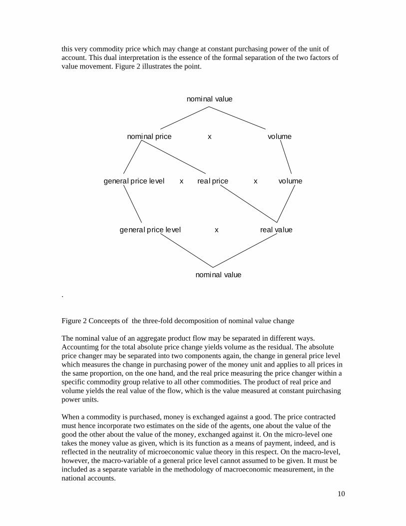
this very commodity price which may change at constant purchasing power of the unit of account. This dual interpretation is the essence of the formal separation of the two factors of value movement. Figure 2 illustrates the point.

.

nominal value

nominal price x volume

general price level x real price x volume

general price level x real value

nominal value

Figure 2 Conceepts of the three-fold decomposition of nominal value change The nominal value of an aggregate product flow may be separated in different ways. Accountimg for the total absolute price change yields volume as the residual. The absolute price changer may be separated into two components again, the change in general price level which measures the change in purchasing power of the money unit and applies to all prices in the same proportion, on the one hand, and the real price measuring the price changer within a specific commodity group relative to all other commodities. The product of real price and volume yields the real value of the flow, which is the value measured at constant puirchasing power units.

When a commodity is purchased, money is exchanged against a good. The price contracted must hence incorporate two estimates on the side of the agents, one about the value of the good the other about the value of the money, exchanged against it. On the micro-level one takes the money value as given, which is its function as a means of payment, indeed, and is reflected in the neutrality of microeconomic value theory in this respect. On the macro-level, however, the macro-variable of a general price level cannot assumed to be given. It must be included as a separate variable in the methodology of macroeconomic measurement, in the national accounts.

11

4. Numerical approximation Differential algebra, while practical as a tool for handling the dynamics of a system in theory, in the actual measurement of variables, it cannot always be applied so easily. When the means to operate in very small intervals of time are not available one has to resort to difference equations, approximating the differential variations. This condition is certainly true for the national accounts. The data they rely on are collected in periods between one month (for some price and production statistics) and ten years (for a population census). As a compromise the year has become the traditional interval for establishing the national accounts at large, parts of them being compiled at quarterly or even monthly („high frequency GDP“) intervals. Applying the differential expressions of the previous section to national accounting is an ordinary problem of numerical approximation, in mathematics. Decisions taken in this field are typically based on good judgement and experience, rather than theory, searching for the best approximation to the true movement, expected in theory. But how good a formula approximates the continuous function depends on the particular shape of the function, of course. The shape not being known in advance, the topic is open to debate and scientific controversy (Stuvel 1989). In this paper we do not enter into the arena, restricting ourselves to a few comments in the direction. Although the proposed tri-partition of value affects all discrete index number decomposition whatever be their individual form, we apply only one of the many options available, relying on the fact that it is widely used, for justification. All we want to show is, how the tri-partition of value may be applied to the national accounts, in principle, leaving details and controversial issues to later discussion. The method employed in national accounts, and in price statistics alike, for approximating the continuous movement of values in time and its decomposition has remained more or less the same, since its inception in the late 19th century (Laspeyres 1971, Paasche 1974). One keeps one of the variables constant over a certain interval of time, varying the other for comparison. In doing so, as the expert puts it, „slight deviations between the assumptions for the index number and reality due to small changes in the expenditure structure of households may be admitted. Only after a stronger cumulation of such deviations should the commodity baskets be modernised, because then the lack of compatibility with the reality of consumption overrules the advantage of showing pure price movements.“ (Guckes 1964, p.435, translation by the author). Thus one measures prices at constant volumes, and volumes at constant prices, for a certain time intervall. When the actual time has moved too far away from the base year, one shifts the base year ahead, connecting it to the previous period by chaining in order to contruct long time series. During most of the 20th century the constant time interval was kept at around five years. With data collection becoming more regular and frequent, and precision requirements became more stringent (Boskin et al. 1997), this interval has been shortened to one year. Let Vi0 be the value of an economic flow in the beginning of a certain time interval (base year) and Vi1 the value at the end (current year). Let Pi0 and Pi1 be the corresponding price indices, so that we have (29) 0000 iiii VQPV = and

12

(30) 0111 iiii VQPV = We may then decompose the nominal growth over the interval by adding and subtracting new terms leaving the total unchanged, (31) ( ) 00010101101 iiiiiiiiiiii VQPQPQPQPVVV −+−=−=∆ . Applying the same difference symbol to volume and price and regrouping yields (32) ( ) 001 iiiiii VQPPQV ∆+∆=∆ . The change in volume is valued at base year price, while the change in price is valued at current year volumes. Doing the reverse is also possible, of course, but national accounts prefer the first method, which may be given a small economic rationale. Market participants are supposed to react to given prices. Thus the volume change is measured in these terms, while the new volumes will then drive prices The aggregate changes are found by summation over all n product classes i, namely (33) ( ) 010 VPQQPVV i ∆+∆=∆=∆ ∑ with (34) ∑ ∆=∆ ii QPQP 00 and (35) ∑ ∆=∆ ii PQPQ 11 . Decomposition 33 is equivalent to defining the index numbers in the following way:

(36) 10

11

0

1

ii

ii

QPQP

PP

∑∑=

(37) 00

10

0

1

ii

ii

QPQP

QQ

∑∑=

which repeats the fact that prices are measured in volumes of the current period and volumes in prices of the base period. In allowing for inflation as a separate monetary effect we now introduce a new independent variable Λ into the decomposition as a third term. The nominal price index 1iP of equation 30 is considered a compound variable depending on real price 1iP and general price level 1Λ according to (38) ii PP Λ=

13

Hence equation 30 becomes (39) 01111 iiii VQPV Λ= . The general price level change affects all transactions equally, it bears no subscript for commodity specifics, therefore. The same technique of decomposition as above (equation 31) applies now to the three-fold set of variables, which leads to

(40)

000010

010011

011111

Λ−Λ+

Λ−Λ+

Λ−Λ=∆

iiii

iiii

iiiii

QPQPQPQP

QPQPV.

This simplifies to (41) QPPQQPV iiiiii ∆Λ+∆Λ+∆Λ=∆ 000111 . Aggregation is again straight forward. We have (42) ( ) 0110100 VQPPQQPVV i ∆Λ+∆Λ+∆Λ=∆=∆ ∑ mit (43) ∑ ∆=∆ ii QPQP 00 (44) ∑ ∆=∆ ii PQPQ 11 (45) ∑= 1111 ii QPQP The first term in the brackets of equation 42 describes the growth of the aggregate in volume, the second in its price relative to the aggregate chosen as standard, and the third term describes the change due to inflation. The decomposition yields the index number formulas

(46) 10

11

0

1

ii

ii

QPQP

PP

∑∑=

(47) 00

10

0

1

ii

ii

QPQP

QQ

∑∑=

(48) 10

11

0

1

iY

i

iY

i

QPQP

∑∑=

ΛΛ ,

where YQ is the volume component of GDP Actually, with three sets of variables there are now six possible ways of decomposing equation 39 (Balk 2003). We have chosen one that shows the change in volume at constant prices as is customary in national accounts, and the specific and the general price level

14

changes together in current volumes, which also corresponds to national accounting practice, and its GDP deflator. We repeat the proof that the real price remains constant if the aggregate V is itself the standard of the general price level (e.g. GDP). From equation 39 we have

(49) 10

11

0

1

10

11

ii

ii

ii

ii

QPQP

QPQP

∑∑

∑∑ =

ΛΛ .

Under the assumption of identical volumes, equations 48 and 49 coincide implying

(50) 110

11

0

1 ==∑∑

ii

ii

QPQP

PP .

5. Path dependence of integrals: mathematics It is generally agreed in macroeconomics that the size of an economy is measured by its gross domestic product (GDP). In describing and analyzing the movement of this variable over time in theory (section2) we have considered time intervals approaching zero in the limit, or at least being so small that variation of one variable may be neglected while varying the other, within the desired degree of measurement precision. Differential analysis yields rates of growth, rates of inflation and the like. Having explained our project of a tri-partition of value at the macroeconomic level in these terms, the question arises about how to integrate such differentials. Integration is summation so that there are actually no particularities to be concerned about, as long as you remain within the chosen intervall (t0, t1). This is the longstanding practice of dealing „in constant prices“. It is only when you transgress the initial time intervall, shift the base year forward, and link it to the time series of the previous base year that a peculiarity of integration arises, called path dependence. As long as the constant price interval was kept for 5 years or longer, the problem was not severe and hardly noticed. But with the new practice, recommended by the SNA world-wide, of shortening the time interval to one year and chaining every year the problem has become acute, and we must answer it within the proposed triadic concept of GDP. Path dependence is a mathematical term having been invented in the 19th century and applied to mechanics and thermodynamics since (Reif 1985). Economics rediscovered it in the 20th century, and it is now a serious issue in growth theory.3 It is related to the fact that to every well behaved cardinal function of more than one variable the partial differentials exist, but not the other way around, necessarily. Not every well behaved function may be integrated to a function of which it is the differential. Precisely, let dV be a differential function of two variables P and Q, so that (51) dQQPhdPQPgdV ),(),( += .

3 The mutual ignorance of the two disciplines using the same mathematics is signified by a double translation in German. What has been called „Wegabhängigkeit“ in the natural sciences for decades is rediscovered as „Pfadabhängigkeit“ in economics, now.

15

The question then is whether the integral over a finite span of time (0, t) exists as an explicit function f(P,Q), so that

(52) [ ] [ ])0(),0()(),(),(),(000

QPftQtPfdQQPhdPQPgdVttt

−=+= ∫∫∫ .

If the integrating function f(P,Q) exists, the value of the integral of dV depends on the values of P and Q at the boundaries of the intervall (0,t) alone. It is called a state function, because it describes a state of the measured object, fully dependent on the independent variables. If an integrating function does not exist there may be other intervening variables not covered by the functions g and h and the result of integration may depend on the particular path P(τ), Q(τ) chosen for integration. In the latter case no certain, path-independent value of the integral exists. If the integral exists, dV in equation 51 is called a total differential, and as a consequence any line integral over an arbitrarily chosen closed path vanishes (Duschek 1958, p.197), (53) ∫ ∫ =+= 0]),(),([ dQQPhdPQPgdV In contrast, if the integrating function f(P,Q) does not exist, the differential dV is incomplete, the value of the line integral is path dependent and not necessarily zero over a closed path. What are the conditions for path independency? From the theorem of Schwarz4 it is known that if there is a continuous function f(P,Q) and functions g(P,Q) and h(P,Q) are its partial derivatives of first order with respect to P and Q, its mixed derivatives of second order are equal: If

(54) Q

P

fQPhfQPg

==

),(),(

then (55) QPPQPQ fhgf === . Hence equation 55 is a necessary condition for an integrating function f(P,Q) to exist. It can also be shown that the reverse is true. Equation 55 is also a sufficient condition for an integrating function to exist, and integration to be path independent (Duschek 1958, p.199). For example, let be in equation 51

(56) PQPhQQPg

==

),(),(

Differentials 55 then read

4 Hermann Amandus Schwarz (1843-1921) was a mathematician teaching at Zürich, Göttingen and Berlin (Duschek 1958, p.44).

16

(57) 1

1

=

=

P

Q

h

g

The integrability condition is fulfilled, there exists an intgrating function f(P,Q), and it is (58) QPQPfV ×== ),( , as can be verified by differentiation. Thus if you know the values of P and Q at times 0 and t, you can calculate the state of V at those times, without considering a path of integration in between. In contrast, assume

(59) .0),(

),(==

QPhQQPg

This results in

0

1

=

=

P

Q

h

g

The cross derivatives are unequal, there exists no integrating function and the integral dV depends in its value on the path )(PQ chosen for integration. (60) ∫ ∫== dPPQdVV )( In order to show this assume you want to integrate the differential function 59 between the points (0,0) and (1,1). If we first move P and then Q we have

(61) 00

),(),(

=+=

+=

∫∫∫ ∫∫

dQdPQ

dQQPhdPQPgdV

along the path (0,0) - (1,0) - (1,1). If, however, we choose the path (0,0) - (0,1) - (1,1) for integration implying that we first move Q and then P we obtain (62) ∫∫∫ =+= 110 dPdQdV . In contrast, doing the same exercise with differentials 57 yields identical integration values for all paths of integration. In equation 51 the nominal value change dV has been decomposed in an additive way, the resulting two components being path dependent. There is a way to decompose them into path independent components by switching to logarithms. Let lower case letters denote logarithms of their respective variables, we may then replace equation 58 by (63) dv = dp + dq.

17

Here we have (64) g(p,q) = h(p,q) =1 and (65) gq =hp = 0, which proves that the mutliplcative decomposition yields two path-independent components. This observation will be used later. 6. Path dependence of aggregates: economics Path dependency is not an issue in economics as long as one deals with figures „at constant prices“, because under that condition path dependency does not occur. To show this let the differential functions be (66) g(P,Q) = 0 h(P,Q) = P0 wirh P0 representing a constant price independent of time. The cross derivatives are then (67) hP = 0 = gQ . The integrability condition is met and we have (68) ∫ ∫ −== )( 0100 QQPdQPdV for any path of integration.Values at constant prices („volumes“) are path independent. Path dependences, therefore, does not occur, as long as you work with a long time interval of five or ten years, allowing volume 10 QQQ ≤≤ alone to vary within the interval. Yearly chaining, - as against 5 year chaining, - does not create the problem of path dependence, but it highlights it, and moves it up to the front of the theoretical agenda. With the advent of short term chaining the counterfactual assumption of constant prices has been corrected in favor of a modern version of prices as „ceteris paribus“ condition, meaning that prices are held constant for an infinitely small time interval only. But this advance in statistical practice has brought up path dependence as an issue to be concerned with, if not in practice, because deviations are small, but in theory. Can path dependent aggregates define meaningfull macroeconomic variables? In the following we will not unroll the path dependence issue in its full history and theoretical diversity (Reich 2004). We only show the light thrown on it if nominal value changes are separated into three components instead of two. In the traditional bi-partite approach, an aggregate V is composed of n prices niPi ,...,1, = and n quantities niQi ,...,1, = altogether 2n independent variables,5 so that

5 Actually the independent variables are Vi and Pi and Qi is being derived, as explained earlier, but in index number theory the derived variables Qi have always been taken as independent and interpreted as quantities.

18

(69) i

n

iiQPV ∑

=

=1

.

In the tri-partite approach an additional variable Λ enters into the computation measuring the change in the accounting unit. So we now have 2n + 1 independent variables. This has a significant effect on the issue of path dependence as we are going to show now. In the bi-partite approach the decomposition of a nominal aggregate value change reads

(70) ∑∑==

+=n

iii

n

iii dQPdPQdV

11

so that

(71) ∑=

=n

iiidPQQdP

1

and

(72) ∑=

=n

iii dQPPdQ

1

are the aggregate components of volume change and price change respectively. These are three differential functions of the 2n variables Pi and Qi where the first one (70) of nominal change is path independent, while the two others of aggregate volume change (71) and aggregate price change (72) are path dependent. Applying condition 55 we find for definition 70

(73) iiii

iiii

PQPhQQPg

==

),(),(

for the 2n derivatives of first order. Forming the derivatives of second order one obtains

(74)

1

,0

0

=

≠==

==

i

i

i

j

j

i

i

j

j

i

Qg

jiQg

Qg

Pg

Pg

∂∂

∂∂

∂∂

∂∂

∂∂

and

Since for the present argument the difference does not matter we follow the traditional approach.

19

(75)

1

,0

0

=

≠==

==

i

i

i

j

j

i

i

j

j

i

Ph

jiPh

Ph

Qh

Qh

∂∂

∂∂

∂∂

∂∂

∂∂

Thus all cross-derivatives of second order are equal and equation 70 is a total differential of the integrating function 12, which is trivial, as it has been derived from equation 69 by differentiation. The same is not true, however, for the aggregate components 71 and 72. The first derivatives of definition 71 are

(76) 0),(

),(==

iii

iiii

QPhQQPg

which yields

(77) 01 =≠=i

i

i

i

Ph

Qg

∂∂

∂∂

Some cross derivatives are unequal, hence the integrating function does not exist, and the integral is path dependent. Similarly for definition 72. Why is path dependence critical in economic terms? The answer is given by the meaning attached to definitions 71 and 72. Equation 71 is interpreted as describing the change in the price level of an economy and equation 72 describes an economy’s growth. If the integral of these changes depends on the path along which an economy develops, their values are ambiguous. Two economies may start from the same set of prices and quantities, arrive at the same set of the variables after some finite time intervall and yet show different price levels and production levels at the end. The very concept of a production function becomes questionable at that point. Growth and inflation are usually expressed as rates of change rather than change in absolute differentials. Defining expenditure shares Si as

(78) SP Q

P Qii i

j j

=∑

so that

(79) ∑=

=n

iiS

11,

and using a lower case letter for the logarithmic derivative, equations 71 and 72 yield (80) ∑= iidpSdp

20

(81) ∑= iidqSdq . Thus the overall rate of inflation is derived as the weighted average of price changes in each product group, and the overall growth is the weighted average of the growth rates of each product class. However, neither differential is a total one, their integration is path dependent (Hulten 1973). Turning to the tri-partite decomposition, we now deal with logarithms of real price changes

ip , and of the general price level λ , instead of nominal prices ip The shares Si remain unchanged if we use real prices instead of nominal prices. Thus we write

(82) λ

λ

dpddqS

dSpdSqdSdv

ii

n

ii

n

ii

n

iiii

n

ii

++=

++=

∑

∑∑∑

=

===

)(1

111

which results in (83) λdvddv += Thus if a nominal aggregate is decomposed into multiplicative components of real value and price level, these two components are path independent, and we may rightly speak of a price level in the sense of describing a state variable of the economy and also of a level of GDP. 7. Conclusion: The foundation of macroeconomics in economic statistics Real value equals nominal value divided by the general price level. Textbooks of macroeconomics have always had a preference for the simple formula of deflation, to the distress of those whose laborious job it is to construct an empirical meaning behind the mathematical symbol. Our analysis provides a justification for the convenient short cut, on the condition that it is properly interpreted. The general price level, in spite of its being expressed as an average of specific price changes, does not address any commodity market at all, but reflects a change in money “value”, so to speak. It expresses a monetary phenomenon. But there is more to be learned from introducing the general price level as an independent variable in macroeconomic analysis. We learn that nominal prices are not “atomic” (indivisible) elements, but compound variables. They are the result of specific market forces in the interaction between supply and demand, on the one hand. On the other hand, these forces work on the basis of a general measurement unit, which makes commodities universally comparable all through the economy over which the currency unit rules. The unit is subject to change over time, itself. The change is revealed as a joint inflation or deflation of all prices in equal proportions, and does not express any commodity market’s forces. It is generally assumed that the state of an economy is fully described by prices and quantities of goods and services produced. Our analysis points out that the measurement unit must be defined in addition. In other words, nominal prices and quantities being the same does not fully determine the state of an economy. You must also know the general price level. As pointed out before, the idea of tri-partitioning nominal value change is not new. Formally,

21

it has been investigated by Stuvel under the heading of price structure vs. price movement. Stuvel sketches a whole system of accounts analyzed in this way (Stuvel 1993, pp. 62ff). Stuvel, however, does not see there is a difference in concepts, namely the price structure referring to what is actually the price of a commodity determined by supply and demand while the general price level is a financial phenomenon. Neubauer (1978), on the other hand, coming from the other end, has criticised the meaning of double deflated value added, arguing for a uniform deflator, instead. The conceptual distinction is also found in the SNA93 as the distinction between “volume”, deflated by its specific price index, and “real value”, deflated by a uniform price index (SNA93, chapter XVI). Stuvel’s formal approach is useful, because it places the analysis within a wider field of empirical investigation, where effects of structure and of level are to be separated. Keeping this broad background in mind helps avoiding the impression that index number problems are of some particular kin not found elsewhere in economic statistics. Neubauer’s and the SNA’s conceptual distinctions clarify the meaning of different deflation procedures, and in this paper we have combined the two ideas. The relevance for macroeconomics at large may be demonstrated by a few examples. Our analysis shows that introducing the general price level as an independent variable in index numbers makes GDP and the general price level independent of their growth paths. The significance of the fact may not be great numerically, where growths paths develop in similar ways, but for the conceptual foundation of theory, it is important. How could you do – to quote one case – “Keynesian Macroeconomics without LM curve” (Romer 2000), in an “output – price level space” (p.152), if both these variables were not describing a state of the economy, but depended in their present value on data of earlier periods? According the general price level an independent variable status secures the meaning of GDP (which is not equal to output, incidentally, in correct SNA terminology) and prices levels in their representations as geometric length on a two-dimensional sheet of paper. In contrast, in drawing such graphs one uses the assumption of path independence, implicitly, and statistical measurement is required to perform along these lines. Taking the analysis one step further, Romer points out as one of his key fundamental choices the dispense with microeconomic foundations (9. 152). Making the general price level an independent variable, revealed in the movement of nominal prices, has the same implication. The controversy is situated around the concept of purchasing power of money. According to microeconomic theory where an objective measure of value is impossible, by definition, purchasing power does not exist. In macroeconomics, however, in practice and in theory, such a variable is inevitable if you want to compare economies over space and time. It is a statistical construct for the money side of an economy, surely, but in this quality it is no worse than the GDP is for the product side, which, like capital, is also not a microeconomic concept (Cohen and Harcourt 2003). Our stance against microeconomic theory as the proper foundation of macroeconomics does not imply non-existence of such foundation. Macroeconomics uses variables form the national accounts, and these are firmly rooted in the concepts of institutional unit and transaction at the micro-level. The required aggregator function must not be searched, or properly defined, it is already there in the accounting methods of business, government, and the national accounts at large. The undisputable microeconomic foundation of macroeconomic theory are the national accounts. Macroeconomics does not fail if it contradicts microeconomic theory, it does if it contradicts the national accounts.

22

For the national accounts themselves the implications of the fore-going analysis are not revolutionary, and included in present practice already. Thus, as it is generally accepted that nominal GDP figures must not be compared directly or added for consecutive years. It would be desirable to present the corresponding general price levels together with GDP figures in tables where the nominal values are put side by side for different years. In this way one would explicitly recognise the variation of the measuring rod of GDP, and warn users. It is new, for the United States, at least, to differentiate between real value and volume for product transactions. The cut helps to distinguish the forces of production from those of exchange in value added. Volume shows production, real value shows production plus exchange. From it follows a theoretical preference for the specific commodity basket chosen for measuring the general price level. Two are in use, the consumer price index, and the GDP-deflator. While the first is closer to market transactions, and appropriate for determining the real wage, the second is more fitting to serve as a unit of account. For it assures consistency between the two core variables of economic growth and monetary inflation within the accounting framework. Both variables are then path independent and variables of state. Furthermore, choosing GDP as the measuring rod of money implies that its real price change is zero, by definition. More precisely, the relative price movements of its components are forced to add to zero. Hence its real value change is due to volume change exclusively, signifying a pure change in production. This falls in line with the general rule of national accounts that all income originates in production, and only there. Within the commodity flow approach fostered by BEA (Popkin 2000) it is then possible, within GDP, to separate the change in the terms of trade of a particular industry from its productivity change, both of which together determine the income accruing to an industry from its activity. Last not least price statistics itself may recognize that the unit of account in which it measures is subject to endogenous variation over time, and add time series of real prices allowing for the bias to their nominal ones. This seems an easy, costless extension of data presentation the user might appreciate. References Balk, Bert M. (2003), “Ideal Indices and Indicators for Two or More Factors,” Research Paper No 0306, Statistics Netherlands, March 10. Balk, Bert M., Rolf Fähre and Shawna Grosskopf (2004), “The Theory of Economic Price and Quantity Indicators,” Economic Theory, 23, pp. 149-164. Barsky, Robert.B. and Lutz Kilian (2004), “Oil and the Macroeconomy Since the 1970s,” Journal of Economic Perspectives, 18, pp. 115-134. Boskin, Michael J., Ellen R. Dulberger, Robert J. Gordon, Zvi Griliches, Dale Jorgenson (1997), “Toward a More Accurate Measure of the Cost of Living,” in Dean Baker (ed.), Getting Prices Right. The Debate Over the Consumer Price Index, Amonk, NY: Sharpe, pp. 15-49.

23

Cohen, Avi J. and G.C . Harcourt (2003), “Whatever happened to the Cambridge Capital Theory Controversies?” Journal of Economic Perspectives, 17 (1), pp.199-214. Duschek, Adalbert (1958), “Vorlesungen über höhere Mathematik,” Zweiter Band, Integration und Differentiation der Funktionen von mehreren Veränderlichen, Wien: Springer. Guckes, Siegfried (1964), „Der neue Preisindex für die Lebenshaltung,“ in Wirtschaft und Statistik, pp. 435-443. Hillinger, Claude (2001)., “On Chained Price and Quantity Measures that are Additively Consistent,” Journal of Economic and Social Measurement, 28. Hulten, Charles R. (1973), “Divisia Index Numbers,” in Econometrica, 41, pp.1017-1025. Koch, Eckard (1998), “Internationale Wirtschaftsbeziehungen,” Band 2, München:Vahlen. Laspeyres, E. (1871), “Die Berechnung einer mittleren Warenpreissteigerung,” Jahrbücher für Nationalökonomie und Statistik, 16, pp. 296-309. Lippe, Peter von der (2000), “Der Unsinn von Kettenindices,” Allgemeines Statistisches Archiv, 84, pp. 67-82. Neubauer, Werner (1978), “Reales Inlandsprodukt: “preisbereinigt” oder “inflationsbereinigt”? Zur Deflationierung bei veränderter Preisstruktur,“ Allgemeines Statistisches Archiv, 62, pp. 115-160. Paasche, H. (1874), Über die Preisentwicklung der letzten Jahre nach den Hamburger Börsennotierungen,” in Jahrbücher für Nationalökonomie und Statistik, 23, pp. 168-178. Popkin, Joel, „The U.S. National Income and Product Accounts,“ Journal of Economic Perspectives, 14 (2), pp. 215-224. Reich, Utz-Peter (2001), “National Accounts and Economic Value. A Study in Concepts,” Basingstoke: Palgrave. Reich, Utz-Peter (2004), “Path Dependence of the General Price Level: A Value-theoretic Analysis”, in Review of Income and Wealth, 50(2), pp. 229-242. Reif, Frederick (1985), “Statistische Physik und Theorie der Wärme,“ Berlin, New York: Walter de Gruyter (translated from „Fundamentals of Statistical and Thermal Physics,“ New York:Mc Graw Hill, 1965). Ricardo, David (1952), „Ricardo to Mill,“ in The Works and Correspondence of David Ricardo, edited by Pierro Sraffa with the collaboration of F. H. Dobb, Volume IX, Letters July 1821-1823, Cambridge, UK: University Press, pp. 385-387 Romer, David (2000), “Keynesian Macroeconomics without the LM Curve,” in Journal of Economic Perspectives, 14 (2), pp. 149-169.

24

Stuvel, Gerhard (1989), “The Index-Number Problem and its Solution”, Basingstoke: Macmillan. Stuvel, Gerhard (1993), “National Accounts Analysis”, Basingstoke: Macmillan. United Nations (1993), “System of National Accounts 1993”, New York, NY.