“Very true,” said the Duchess: “flamingoes and mustard

BIOSTATS 540 – Fall 2021 Course Introduction Page 1 of 19

Nature Population/ Sample

Observation/ Data

Relationships/ Modeling

Analysis/ Synthesis

Course Introduction

“Very true,” said the Duchess: “flamingoes and mustard both bite. And the moral of that is – “’Birds of a feather flock together. ‘ “

“Only mustard isn’t a bird,” Alice remarked. “Right, as usual,” said the Duchess: “what a clever way you have of putting things!”

- Alice in Wonderland

Welcome to BIOSTATS 540, Fall 2021. These notes begin with a description of the “road map” that you see in the footer of each page. This is followed by a brief introduction to statistical thinking using some examples; they remind us of the ways in which we are poor at evaluating probability. Perhaps this is a good place to start our work? I then provide a brief overview of each unit.



Observation/ Data


Analysis/ Synthesis

Cheers!

Source: Landers JB (www.landers.co.uk)



Observation/ Data


Analysis/ Synthesis

Table of Contents

Topic

1. Course Roadmap …………………………….……………………………. 2. A Feel for Things ………………………………….……………….……. 3. Overview, Unit by Unit …………………………………….………...……

4 6 12

Key Points ……………………………………………………….……………...

19



Observation/ Data


Analysis/ Synthesis

1. Course Roadmap

Nature

Nature is full of variation. Variation might be from time to time, from person to person, or from replicate to replicate. Or, it might be from one treatment to the next or from one exposure to the next. Which variations are “real”, representing differences that are systematic in some knowable way, and which variations are “noise”, representing what we call natural or random variation which we think of (for the moment anyway) as “noise”? Do we even know what we’re talking about when we distinguish “real” from “random”?

Populations/

Sample

A population is a collection of some sort of entirety (however that might be defined) of individuals. An example is the collection of individuals who will actually vote in the 2020 U.S. elections. Numerical facts about a population are called parameters. If we could study a population by examining each and every member, we would be doing a census. This course is not about censuses. More often, what is available to us is limited to just a selected subset of a population; that selected subset is called a sample. Numerical facts about a sample are called statistics. We can calculate these! Values of statistics from a sample are often used as guesses about the population from which the sample was obtained provided the method of sampling was appropriate (more on this later). This is called inference.

Observation/

Data

Observation and data may not be the same. What does your mind’s eye “register” when you observe a flower? A lot, actually. However, in your description, you will report only some of what you have observed; e.g., the flower as red, with 5 petals, and having a strong aroma. “Red”, “5 petals”, “strong aroma” are your data. Data are the result of selection (which attributes of the flower did you choose to note?) and measurement (what value scheme are you using?). Just think of the many attributes of the flower that were not selected as your data! A variable is a characteristic or attribute; it is something whose value can vary. Data are the values you obtain by measurement of the variable. “Color” is a variable. “Red” is a data value.



Observation/ Data


Analysis/ Synthesis

Relationships/ Model

A relationship exists between two variables if they co-vary (e.g., – increasing (excessive) sun exposure is accompanied by increasing numbers of events of skin cancer) Statistical modeling is used to discover relationships. An important perspective is the following. The starting point is some data and our goal is to describe it well. To do so, we entertain some models that might be a good fit. Eventually, we settle on one that we believe is a “good model”. But there may be (and probably are!) several models that describe a given set of data well. A good model is one that (i) explains a good amount of the variability in the data (adequacy); and is then (ii) minimally adequate (parsimony), meaning: it represents your best understanding of the factors that are related to your response variable while, at the same time, being as simple as possible.

Analysis/ Synthesis

The observation of a relationship does not mean there is causality (e.g. – ice cream sales and murder rate, except when they’re out of mocha chip, just kidding…)



Observation/ Data


Analysis/ Synthesis

2. A Feel for Things A variety of illustrations provide a feel for things. Example – Genetic Counseling A couple has a baby with a genetic defect. They are considering having another baby. What is the likelihood that the second child will have a genetic defect also? Example 1 – Prognosis A physician is considering several therapies for the treatment of a patient. Which therapy should be used? Each therapy produces a result that is somewhere between success and failure. The final choice of therapy is “weighed” against the others, according to the anticipated outcomes. (Yes, you’re right. The weights might be the probabilities themselves)

Probabilities are a tool in decision-making.

Example 2 – Federal Drug Testing Is a food additive carcinogenic? An investigator explores this in an experiment that compares two groups: “controls” and “treated”. Only some of the controls develop cancer and only some of the treated individuals develop cancer. But, perhaps, a greater percent of the “treated” individuals develop cancer. Is the excess number of cancers among treated individuals meaningful, that is: is the excess of cases among “treated” individuals, relative to the number of cases among the controls, beyond what we might have anticipated by chance?



Observation/ Data


Analysis/ Synthesis

Example 3 – Smoking and Cancer Lung cancer occurs only sometimes. It is not an invariable consequence of smoking. Interest is identifying the factors related to a variable outcome.

Statistical inference about associations is not equivalent to the understanding of deterministic phenomena

(association ≠ causation).

Example 4 – Justice versus Medicine In the judicial system, we say “innocent until proven guilty” (Quick check - do you agree with this “bias”?)

- If it’s possible to be wrong, we’d rather err in the direction of “letting go free” a guilty person. In the practice of medicine, we say it is “better to order another test” (How about here - do you agree with this “bias”?) - Again, if it’s possible to be wrong, we’d rather err in the direction of suspecting disease.

Accepted and known biases influence decision-making

(Quick question for you. Would you say that we all view the world through tinted lenses?)



Observation/ Data


Analysis/ Synthesis

Example 5 – Investigation of the Portacaval Shunt Source: Grace, Muench, Chalmers (1966) summarized the findings in over 50 studies of what was, at the time, a new surgical treatment (portacaval shunt) for advanced liver disease. The authors’ conclusion (specifically their level of enthusiasm for the shunt procedure) were classified according to study design.

Reported Enthusiasm for Shunt Marked Moderate None Design

No controls 24 (75%) 7 1 Observational Controlled 10 (67%) 3 2

Randomized Trial

0 (0%) 1 4

Wow. 75% markedly enthusiastic for the “no control” studies versus 67% markedly enthusiastic for the “observational control” studies versus 0% markedly enthusiastic for the “randomized controlled trials”. What’s going on “under the hood” to explain why the percentages (75% versus 67% versus 0%) are so different? The answer might lie in unknown biases, in contrast to what we saw in example 4. Since 1966, we have seen the increasing use of randomization designs.

Unknown biases influence decision making

Example 6 – Is living near electricity transmission equipment associated with occurrence of cancer?

Cancer Not Lives near equipment 200 1646 11%

Lives elsewhere 50 7289 1% Among those living near electricity equipment, 11% have cancer. Among those living elsewhere, only 1% have cancer. 11% versus 1% is potentially a big difference. But is it meaningful? Now suppose that, for these same data, we also have information about asbestos exposure. In particular, suppose we can “partition” the entire data into two subsets, one where exposure to asbestos has occurred and one where it has not occurred. Thus, within each subset, all persons have “similar” levels of exposure (we have “controlled” for asbestos exposure).



Observation/ Data


Analysis/ Synthesis

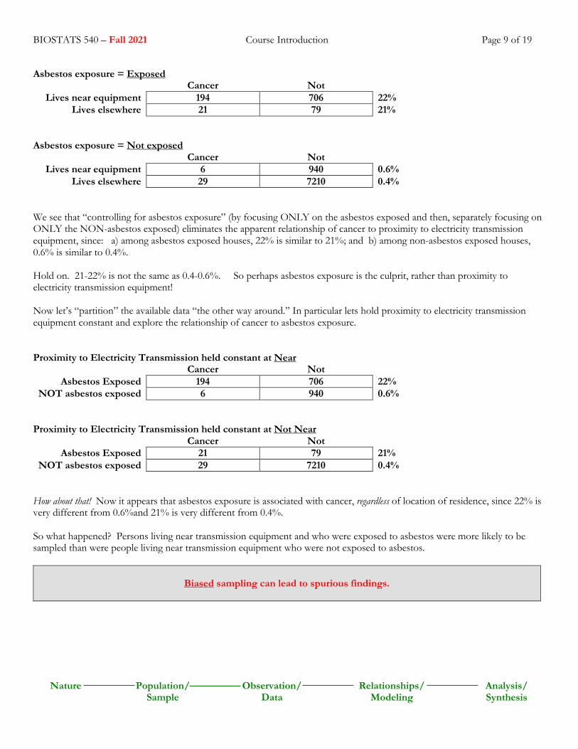
Asbestos exposure = Exposed Cancer Not

Lives near equipment 194 706 22% Lives elsewhere 21 79 21%

Asbestos exposure = Not exposed

Cancer Not Lives near equipment 6 940 0.6%

Lives elsewhere 29 7210 0.4% We see that “controlling for asbestos exposure” (by focusing ONLY on the asbestos exposed and then, separately focusing on ONLY the NON-asbestos exposed) eliminates the apparent relationship of cancer to proximity to electricity transmission equipment, since: a) among asbestos exposed houses, 22% is similar to 21%; and b) among non-asbestos exposed houses, 0.6% is similar to 0.4%. Hold on. 21-22% is not the same as 0.4-0.6%. So perhaps asbestos exposure is the culprit, rather than proximity to electricity transmission equipment! Now let’s “partition” the available data “the other way around.” In particular lets hold proximity to electricity transmission equipment constant and explore the relationship of cancer to asbestos exposure. Proximity to Electricity Transmission held constant at Near

Cancer Not Asbestos Exposed 194 706 22%

NOT asbestos exposed 6 940 0.6% Proximity to Electricity Transmission held constant at Not Near

Cancer Not Asbestos Exposed 21 79 21%

NOT asbestos exposed 29 7210 0.4% How about that! Now it appears that asbestos exposure is associated with cancer, regardless of location of residence, since 22% is very different from 0.6%and 21% is very different from 0.4%. So what happened? Persons living near transmission equipment and who were exposed to asbestos were more likely to be sampled than were people living near transmission equipment who were not exposed to asbestos.

Biased sampling can lead to spurious findings.



Observation/ Data


Analysis/ Synthesis

Putting it all together The information available is often incomplete. Decision making then requires some kind of evaluation of models of probability.

¨ Statistical methodologies are tools for managing these issues One goal is to inform decision making, as in the examples described in previously:

• Family planning • Patient care • Tobacco and lung cancer (Experiment) • Tobacco and lung cancer (Observation)

Uncertainty is not necessarily approached objectively. Again, consider this. We all bring to decision-making settings our “way of thinking”, our “lense”, our “baggage” if you will. Some of these biases are in our awareness and, possibly, are desirable. Others are not. Examples of decision-making settings where there might exist biases that are known and desirable are the following:

• Judicial system (bias: “innocent until proven guilty”) • Diagnostic testing (bias: “when in doubt, continue to suspect disease”) • Type I, II error (stay tuned … we’ll get to this in unit 8, statistical literacy)

An example where the influences are not necessarily in our awareness is the following: • Portacaval shunt Investigators must consider as fully as possible all of the factors which might be related to the observed outcomes. • The transmission equipment, asbestos, cancer example • Experimental design



Observation/ Data


Analysis/ Synthesis

The tools of biostatistics are of two types: - Description - we use the values of statistics (we can calculate these!) from a sample to make estimates about the

corresponding parameter values that characterize a population (which we do NOT know!).

- Inference making - through the fitting and comparison of competing models of the data, we obtain a comparison (hypothesis test) of competing explanations (hypotheses) of the phenomena we have observed.

Example 7 - In 1969, the average number of serious accidents per 1000 workers per year in a large factory was 10. In 2021, the average number of serious accidents per 1000 workers per year in the same factory was 7. Is the downward trend from 10 to 7 real or a reflection of natural variation? Example The spaceship Voyager 2 is circling the planet Uranus. What is the “blip” on our radio receiver here on earth? Is it a true signal? Or, is it random noise such as cosmic rays, magnetic fields, or whatever?

The “signal-to-noise ratio” concept is helpful: Signal - Treatment effect, Exposure effect, Secular trend Noise - Natural variation, Random error Random error is the “noise” in the “signal-to-noise ratio” concept.

Description

Inference Making

Example: From a data set consisting of 573 cholesterol values obtained from a simple random sample of a specified population, calculate the sample mean and use this to obtain an estimate of the unknown population mean cholesterol value.

Example: Is excessive occupational exposure to video display terminals (computer monitors) during pregnancy associated with a greater likelihood of spontaneous abortion?

Solution: Confidence interval for the unknown population mean value. We will learn how to do this in Unit 9, One Sample Inference.

Solution: Two-sample test of equality of occurrence of spontaneous abortion. We will learn how to do this in Unit 10, Two Sample Inference.



Observation/ Data


Analysis/ Synthesis

3. Overview, Unit by Unit

Units 1 & 2 Summarizing Data Data Visualization In these units, you will learn methods for summarizing and visualizing data. These techniques enable us to condense a great amount of data into an easily digested format. This course will emphasize the importance of looking at data. You will gain practice in recognizing the flaws of a bad graph and will learn methods for producing good graphs. Example - Human microarray data were obtained from a sample of n=106 women, representing two groups: 42 nulliparous (never been pregnant) plus 64 parous (history of 1 or more pregnancies). The purpose of the study was to investigate the expression of estrogen receptor alpha (ERS1) and, in particular, how this expression changes with age. A challenge to this analysis, however, is the potential influence of parity on ESR1. In particular, if all the younger women in the sample were nulliparous and all the older women in the sample were parous, it would be impossible to isolate and estimate the effect of age on ESR1, independent from that of parity. Therefore, in a preliminary analysis, a histogram summary of the distribution of age was obtained separately for the nulliparous versus parous subgroups. As expected, the distribution of ages tends to be younger among the nulliparous and older among the parous. Some overlap can be seen but inspection of the counts of women in the overlap suggest that it will be difficult to disentangle the effects of age versus parity on ESR1 expression.



Observation/ Data


Analysis/ Synthesis

Units 3 & 4 - Probability Basics Probabilities in Epidemiology In Unit 3, we will work with the ideas of chance (eg – the chances of a fair coin landing “heads” is 0.50) and the basics of calculating probabilities. This understanding is useful when asking questions such as

• Diagnostic testing What are the chances that a person with a positive test result is truly diseased?

• Clinical Trials What were the chances that the treatment group, relative to the control group, exhibited a more favorable response if in fact the treatment and control therapies are equivalent?

Often, BIOSTATS 540 students don’t like Unit 3; the intuition of probabilities is hard for all of us. Some good news. Unit 3 is not tested and upon arrival to Unit 4, Unit 3 is safely in the review mirror! But Unit 4 (“Probabilities in Epidemiology”) is useful because of its relevance to public health; e.g., as when asking questions such as the following.

Example of diagnostic testing - Suppose it is known that the probability of a positive mammogram is 80% for a woman with breast cancer and is 9.6% for a woman without breast cancer. Suppose further that, in the general population, the chances that an individual will ever develop breast cancer are 1%. If we are told that an individual patient is known to have a positive mammogram, we can use an approach known as Bayes Rule to solve for the probability that she is truly diseased. As we shall see in Unit 4, the answer in this example is that this individual’s chances of cancer, given that she had a positive mammogram, are 7.8% .

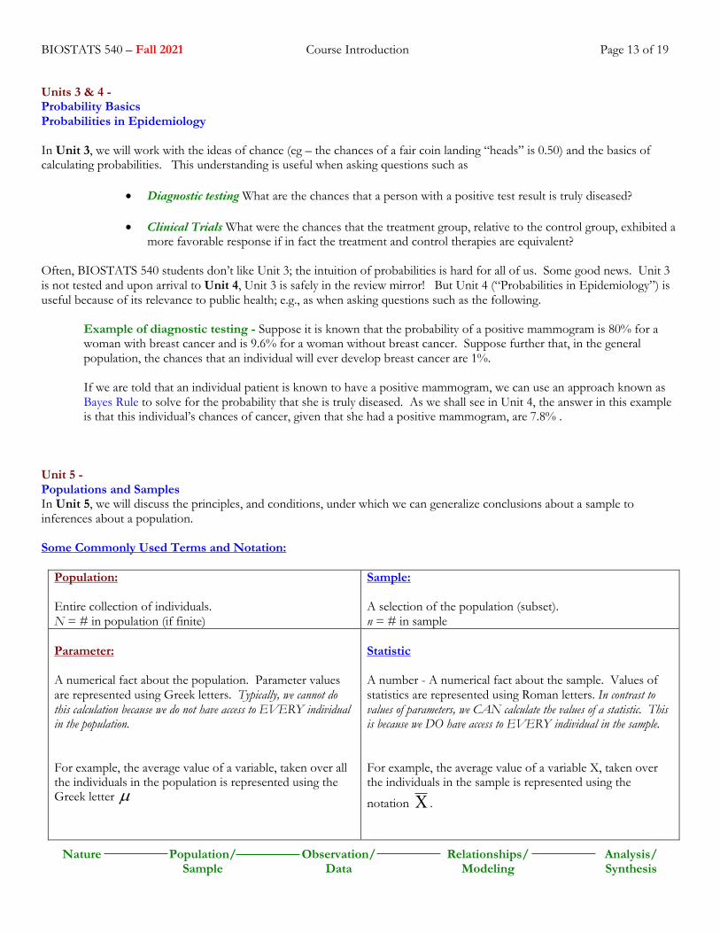
Unit 5 - Populations and Samples In Unit 5, we will discuss the principles, and conditions, under which we can generalize conclusions about a sample to inferences about a population. Some Commonly Used Terms and Notation:

Population: Entire collection of individuals. N = # in population (if finite)

Sample: A selection of the population (subset). n = # in sample

Parameter: A numerical fact about the population. Parameter values are represented using Greek letters. Typically, we cannot do this calculation because we do not have access to EVERY individual in the population. For example, the average value of a variable, taken over all the individuals in the population is represented using the Greek letter

Statistic A number - A numerical fact about the sample. Values of statistics are represented using Roman letters. In contrast to values of parameters, we CAN calculate the values of a statistic. This is because we DO have access to EVERY individual in the sample. For example, the average value of a variable X, taken over the individuals in the sample is represented using the

notation .

µ X



Observation/ Data


Analysis/ Synthesis

Take away – In general, we do not get to see population parameter values. For example, is unknown.

Take away – We do get to see values of statistics. For

example, = 85. The value 85 might be a guess of the unknown .

In Unit 5, we’ll review what it means to draw a simple random sample from a population (think pulling raffle cards out of a hat here). You will also learn that if a sample is not obtained in an appropriate manner (based on a probability model), then it may not be possible to generalize findings from analysis of the sample to inferences about the population.

Example - Since tests of blood lead levels are costly to administer, a simple random sample of n=20 children were selected from the population of N=293 at a particular school. The 20 children in the sample were each given the test. Based on a summarization of their test values, an estimate is made concerning the mean blood lead level of all 293 children in the school.

Units 6 & 7 - Bernoulli and Binomial Distribution Normal Distribution The patterns and variations of occurrence of many phenomena can be described well by imagining that what we’ve observed are random draws from some particular probability model distributions. In Units 6 and 7, you will be introduced to three probability model distributions: Bernoulli, Binomial, and Normal. The Bernoulli (Bernoulli trial) probability model is useful for modeling the pattern of discrete outcomes in one instance where there are only two possible outcomes (eg – “success” or “failure”).

Example - The outcome of tossing a fair coin one time is modeled using the Bernoulli probability model. It says that “heads” occurs with probability 50% and tails occurs with probability 50%. Example - The outcome of occurrence of flu in one person who received a flu shot might be modeled using the Bernoulli probability model. For this coming winter, 2020, it might predict that a randomly selected person who received the flu shot has a 4% chance of succumbing to the flu.

The Binomial probability model is useful for modeling the net result of a multiple number of Bernoulli trials. (eg – “what are the chances of exactly 3 “sixes” (six dots on the face of the die) in 20 rolls of a single die?”).

Example - The probability of obtaining a six in one rolling of a single die is 16.67%. Suppose you roll the single die 20 times. The probabilities of obtaining 0 sixes, 1 six, 2 sixes, etc., is an example of the binomial probability distribution. A graph of this probability distribution is shown below. On the horizontal axis is the number of successes, “x”; thus, x might be 0, 1, 2, … , 20. On the vertical axis is the probability of getting that many (“x”) sixes in 20 rolls. For example, you can see in this graph that the probability of getting x=3 sixes in 20 rolls is .2379, representing a 24% chance approximately.

µ Xµ



Observation/ Data


Analysis/ Synthesis

Source: https://istats.shinyapps.io/BinomialDist/ The Normal (also called Gaussian) probability model is one model that is useful for describing the pattern of outcomes that have values on a continuum (e.g. – cholesterol measurements have values that lie on a continuum)

Example - The pattern of scores on a standard IQ test is well described by a normal probability model distribution. A graph of this probability distribution is shown below. On the horizontal axis, “x1 and x2” refer to two different IQ test scores – 85 and 115, respectively. The values “z1 and z2” below are standardizations of “x1 and x2” and are called standardized z-scores (no worries – we’ll get to this in Unit 7). The smooth bell-shaped curve is called the probability density function. Probabilities here are calculated as areas under this curve. This graph says that the probability is .6826 (representing a 68% chance, approximately) that a randomly sampled individual has an IQ that is between 85 and 115. Much more on this in Unit 7.

Source: http://strader.cehd.tamu.edu/Mathematics/Statistics/NormalCurve/

X = Number of Successes = “number of sixes in 20 rolls of a die”

Probability of 3 “sixes” in 20 rolls of a die = .2379



Observation/ Data


Analysis/ Synthesis

Units 8, 9 & 10 - Statistical Literacy – Introduction to Estimation and Hypothesis Testing One Sample Inference Two Sample Inference In Units 8, 9 & 10, we will learn how to think about statistical estimation and hypothesis testing (this is statistical literacy and is introduced in Unit 8) and will then apply these ideas in one and two sample inference (Units 9 and 10). As an example of statistical literacy, you will learn that saying “the probability is .95 that …” is not the same as saying “I am 95% confident that…”. You will also learn the distinction between “statistical significance” versus “biological significance”.

Example – Do children living in Worcester, MA have healthy LDL levels? A particular school has N= 293 children. On the basis of a simple random sample of size “n=50” children from this school and the measurement of low-density cholesterol (LDL) on each child, it is of interest to estimate the average LDL of all of the 293 children. We might also be interested in assessing (hypothesis testing) whether or not we can reasonably infer that the average level is above some specific value. Hint – one sample confidence interval and hypothesis test (Unit 9). Example – Is childhood exposure to lead associated with lower IQ? A simple random sample of size n1 is drawn from one population (e.g. – toddlers exposed to lead) and a simple random sample of size n2 is drawn from a second, independent, population (e.g. – toddlers with no exposure to lead). On the basis of the information in these two samples, we seek to make some inferences concerning the comparability of the two populations. Hint – two (independent) samples test of equality of means (Unit 10)

Example – Is a particular new drug effective in lowering blood pressure? Suppose a new drug is manufactured for lowering blood pressure. How do we determine if the drug does what is claimed?

Blood Pressure

Subject Before After Difference 1 2

… n

Blood pressure measurements are taken on n subjects before they start taking the new drug, and again on the same subjects after 2 weeks use of the new drug. If the drug is successful we expect the average within-subject difference, before minus after, to be positive. i.e., average of (xi – y i ) > 0 , indicating that there was a drop in blood pressure. Hint – one sample test for paired data (Unit 9)

x1 y1 x y d1 1 1- =x2 y2 x y d2 2 2- =

xn yn x y dn n n- =



Observation/ Data


Analysis/ Synthesis

Unit 11 - Chi Square Tests In Unit 11, we will take a closer look at data that are counts.

Example - Is there any relationship between smoking and death from heart attack? Suppose smoking history, recorded as simply “yes” or “no” is obtained for each of 5000 deaths. Suppose we also have information on cause of deaths and, in particular, whether or not the cause of death was a heart attack. A chi square test would be used to address the question - Is there any relationship between smoking and death from heart attack?

Died of Heart Attack Died of Other Cause

Smoker Death 600 (15%) 3400 4000 Non-smoker Death 50 (5%) 950 1000

5000

In epidemiology parlance, the 2x2 table data are represented using a standard format and layout in which the arrangement of counts is given the particular names “a”, “b”, “c” and “d” as shown below. Thus, in this example of n=5000 deaths, we observe “a=600” deaths due to heart attack among “(a+b)=4000” deaths among smokers. And so on.

Died of Heart Attack Died of Other Cause

Smoker a = 600 b = 3400 (a+b) = 4000 Non-smoker c = 50 d = 950

n = (a+b+c+d)



Observation/ Data


Analysis/ Synthesis

Unit 12 - Regression and Correlation We are often interested in the relationship among several variables computed on the same individual. In Unit 12, you will be introduced to the ideas of modeling (spoiler – we’ll be using the word “modeling” a lot but, in reality, we’ve been modeling all along). Specifically, you will be introduced to simple linear regression and correlation in the setting of a single predictor variable measured on a continuum and a single outcome variable that is also measured on a continuum. In this setting, we will also assume that the pattern of values of the outcome variable is distributed normal. Example - Is there a relationship between weight and age?

¨ The plot suggests a relationship between AGE and WT ¨ Specifically, it suggests that older AGE is associated with higher WT ¨ A straight line might fit well, but another model might be better ¨ We have adequate ranges of values for both AGE and WT ¨ There are no outliers



Observation/ Data


Analysis/ Synthesis

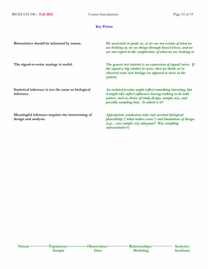
Key Points Biostatistics should be informed by nature.

We need tools to guide us, as we are not certain of what we are looking at, we see things through biased lenses, and we are not expert in the complexities of what we are looking at

The signal-to-noise analogy is useful.

The generic test statistic is an expression of signal/noise. If the signal is big relative to noise, then we think we’ve observed some new biology (as opposed to noise in the system)

Statistical inference is not the same as biological inference.

An isolated p-value might reflect something intersting, but it might also reflect influences having nothing to do with nature, such as choice of study design, sample size, and possibly sampling bias. So which is it?

Meaningful inference requires the intertwining of design and analysis.

Appropriate conclusions take into account biological plausibility (“what makes sense”) and limitations of design (e.g., - was sample size adequate? Was sampling representative?)

Documents

“Very true,” said the Duchess: “flamingoes and mustard