CSEM WP 126R

Vertical Arrangements, Market Structure, and

Competition: An Analysis of Restructured U.S.

Electricity Markets

James Bushnell, Erin T. Mansur, and Celeste Saravia

Revised February 2005

This paper is part of the Center for the Study of Energy Markets (CSEM) Working Paper Series. CSEM is a program of the University of California Energy Institute, a multi-campus research unit of the University of California located on the Berkeley campus.

2547 Channing Way Berkeley, California 94720-5180

www.ucei.org

Vertical Arrangements, Market Structure, and Competition:

An Analysis of Restructured U.S. Electricity Markets

James B. Bushnell, Erin T. Mansur, and Celeste Saravia∗

February 15, 2005

Abstract

This paper examines the relative importance of horizontal market structure, auction de-sign, and vertical arrangements in explaining electricity prices. We define vertical arrange-ments as either vertical integration or long term contracts whereby retail prices are determinedprior to wholesale prices. This is generally the case in electricity markets. These ex ante re-tail price commitments mean that a producer has effectively entered into a forward contractwhen it takes on retail customers. The integrated firm has less incentive to raise wholesaleprices when its sale price is constrained. For three restructured wholesale electricity markets,we simulate two sets of prices that define the bounds on static oligopoly equilibria. Ourfindings suggest that vertical arrangements dramatically affect estimated market outcomes.Simulated prices that assume Cournot behavior but ignore this vertical scope vastly exceedobserved prices. After accounting for the arrangements, performance is similar to Cournotin each market. Our results indicate that auction design has done little to limit strategicbehavior and that horizontal market structure accurately predicts market performance onlywhen vertical structure is also taken into account.JEL Classification: L11, L13, and L94Keywords: Vertical Arrangements, Market Power, Oligopoly, and Electricity Markets

∗Bushnell: University of California Energy Institute. Email: Bushnell@Haas.Berkeley.edu. Mansur: School ofManagement and School of Forestry and Environmental Studies, Yale University. Email: Erin.Mansur@Yale.edu.Saravia: Cornerstone Research. Email: csaravia@cornerstone.com. We thank Soledad Arellano, Severin Boren-stein, Joe Bowring, Judy Chevalier, Stephen Holland, Jun Ishii, Wally Mullin, Steve Puller, Peter Schott, FionaScott Morton, Raphael Thomadsen, Larry White, Matt White, Frank Wolak, and Catherine Wolfram for helpfulcomments.

1

1 Introduction

While rules concerning horizontal market structure form the basis of antitrust policies in most

countries, it is widely recognized that horizontal structure comprises only one piece of the com-

petition puzzle. Vertical integration and other vertical arrangements between wholesalers and

retailers will also impact the incentives of firms. In addition, regulators and many economists

have focused on the effects that auction design may have on equilibrium prices. This paper

empirically examines the relative importance of horizontal market structure, auction design, and

vertical arrangements in determining prices in imperfectly competitive markets.

We study three U.S. electricity markets: California, New England, and the Pennsylvania,

New Jersey, and Maryland (PJM) market. These were the first three U.S. markets to undergo

regulatory restructuring. There is substantial evidence that the California market was the least

competitive.1 However, previous studies do not address why there were apparent differences in

the competitiveness of these markets.

Our analysis highlights the importance of vertical integration and vertical contracts, although

for reasons that have not to date received much treatment in the literature on vertical structure.

The organization of the electricity industry, where distribution is the province of independent

grid operators, reduces the risk of the negative consequences of vertical integration such as fore-

closure or the raising of rivals’ costs. Instead, it is the rigidity of retail prices that creates a

strong relationship between vertical structure and competitive performance. Regulators con-

strain retailers in their ability to adjust electricity prices. The rate-making process restricts the

frequency with which retail prices can be adjusted, usually no more frequently than annually.

This is particularly true during our sample period, where transition arrangements put in place at

the time of restructuring strongly restricted retailer’s ability to adjust prices. Even in completely

deregulated retail markets, however, price-commitments of a year in length are the norm. The

key attribute is that integrated firms are making retail price commitments before committing

1See Borenstein, Bushnell, and Wolak (2002), Bushnell and Saravia (2002), Joskow and Kahn (2002), Mansur(2004), and Puller (2004).

2

production to the wholesale market.

A restriction on retail price adjustment means that a producer is effectively making a long-

term forward commitment when it integrates with downstream retailers. Vertical relationships

take the form of long-term price commitments to retail customers. The integrated firm has

committed to supplying a portion of its output at fixed prices to its retail customers and therefore

has an effectively smaller position on the wholesale market and less incentive to raise wholesale

prices. The impact on the incentives of wholesale producers is analogous to that provided by a

futures contract or other hedging instrument, which is generally thought to be pro-competitive.2

Firms effectively undercut each other in the forward market in an attempt to gain a Stackelberg

leader position.

Many industries exhibit similar vertical relationships whereby the presence of long-term,

fixed price contracts are likely to influence the spot market. Other energy markets—such as

railroad coal deliveries and natural gas—are structured similarly where some of the supply is

procured through long term fixed-price contracts and some through a spot market (or short

term contracts).3 To some degree, many imperfectly competitive industries—including concrete,

construction, telecommunications, and pharmaceuticals—feature both wholesale forward price

commitments and spot markets that foster competition.

We compare the market performance of restructured electricity markets to estimates that ab-

stract away from specific auction rules but capture important structural characteristics. Specif-

ically, we estimate market outcomes under an assumption of perfect competition and under an

assumption of Cournot competition. These two counter-factual assumptions bound the space

of possible static, non-cooperative outcomes. By establishing where actual market outcomes

fall within these bounds, we can compare how markets are performing relative to the extremes

determined by structural factors alone.

2In particular, Allaz and Vila (1993) note that an oligopoly equilibrium will be more competitive when thereare more opportunities for firms to contract ahead of the time of delivery.

3By contrast, in the gasoline industry retailers change prices with impunity and great frequency. Verticalcontracts between refiners and retailers guarantee the supply of physical product, but almost never set an advancedfixed price for that product.

3

In our study, the impact of vertical arrangements on estimated market outcomes is dramatic.

When vertical arrangements are not taken into account, we demonstrate that both Eastern mar-

kets were dramatically more competitive than would be predicted by a model of Cournot competi-

tion. The California market, by contrast, produced prices somewhat lower, but largely consistent

with an assumption of Cournot competition. We use publicly available data on long-term retail

supply arrangements. When these retail obligations are included in the objective functions of

suppliers, Cournot equilibrium prices in both PJM and New England fall substantially.

In each market, actual prices are similar to our simulated prices that assume Cournot behavior

and that account for vertical arrangements. Horizontal structure does explain performance but

only when coupled with these arrangements. After accounting for these structural factors, there

is relatively little variation between markets left to be explained by auction design, market rules,

and other factors. These results support the hypothesis that long-term contracts and other

vertical arrangements are a major source of the differences in performance of electricity markets,

and possibly of other markets with long term contracts also.

This paper proceeds as follows. Section 2 presents our theoretical modeling framework. In

Section 3, we provide a general overview of the relevant characteristics of the three markets we

study. Section 4 describes our model and data. We present our results in Section 5 and state our

conclusions in Section 6.

2 Market Structure and Performance

The design of deregulated electricity markets offers economists a unique and challenging oppor-

tunity. Wilson (2002) discusses the many physical problems inherent in the design of electricity

markets including the necessity of balancing supply and demand instantaneously and the diffi-

culties that transmission congestion offers to the problem. Although market design may have a

large effect on market outcomes, Joskow (2003) notes that the majority of the benefits that result

from a well designed electricity market will be concentrated in the few hours when the market

structure is less favorable to competition. In particular, he states: “All (electricity) wholesale

4

market designs work reasonably well in the short run when demand is low or moderate. The

performance challenges of wholesale market institutions arise during the relatively small number

of hours when demand is high.”

Undoubtedly, the attempts by economists to design well functioning markets that give players

the correct incentives can improve production efficiency and limit market power. However, it

appears that some energy regulators have come to the conclusion that market design is more

important than market structure. This view that regulating market design may be the best

way to proceed is particularly true in electricity markets. For example, in a November 2000

report, the Federal Energy Regulatory Commission (FERC) concluded that the flawed rules of

the California electricity market contributed to the crises in that state.4 The FERC subsequently

proposed a Standard Market Design that it will encourage all deregulated electricity markets to

adopt.5 The FERC has stated that it is willing to trade leniency in its review of market structure

for the voluntary submission of firms to its standardized market rules.6 The focus of electricity

policy makers on market design and the lack of attention given to market structure may be due

in part to the self-professed, but somewhat misguided, inability of regulators to do anything to

improve structural conditions. Evans and Green (2003) address questions of the importance of

market rules in the context of a dramatic rule change in England and Wales. Our approach is

quite different, however.

We measure the impact of vertical and horizontal market structure on market performance.

Our approach is to abstract away from the detailed market rules and regulations in each market

and examine the range of equilibrium price outcomes that would be predicted from considering

market structure alone. We calculate the upper and lower bounds on market prices that could be

produced in a static, non-cooperative equilibrium. These bounds are, respectively, represented

4The FERC found that “electric market structure and market rules for wholesale sales of electricity energy inCalifornia were seriously flawed and that these structures and rules in conjunction with an imbalance of supplyand demand in California have caused and continue to have potential to cause, unjust and unreasonable rates forshort term energy.”

5See Standard Market Design and Structure RM01-12-000 at http://www.ferc.gov/industries/electric/indus-act/smd.asp.

6See Bushnell (2003a) for a discussion of FERC policy initiatives regarding market structure and market design.

5

by the Nash-Cournot and perfectly competitive, or price-taking, equilibria.

Several models of oligopoly competition in the electricity industry have employed the supply

function equilibrium (SFE) concept developed by Klemperer and Meyer (1989).7 In many cases

there exist multiple SFE, and Klemperer and Meyer show that these equilibria are bounded by

the Cournot and competitive equilibria. To the extent that auction design influences market

outcomes by helping determine which of the many possible equilibria arise, these impacts can

be thought of as placing the market price within these bounds.8 Several papers have applied a

model of Cournot competition to electricity markets to forecast possible future market outcomes

using hypothetical market conditions.9 Unlike those papers we are applying actual market data

to simulate market outcomes within the Cournot framework.

The consideration of vertical arrangements is critical to our examination of the interaction

of market structure and prices. The impact of vertical structure on market performance has

been a subject of interest in many industries. Much of the concern about the negative impacts

of vertical arrangements has focused on foreclosure or the ability of the integrated firm to raise

rivals’ costs.10 However, in the markets we study, third party independent system operators

control the common distribution networks. This, combined with the fact that electricity is a

homogenous commodity makes it somewhat more difficult for suppliers to foreclose competitors

or discriminate in favor of their own retail affiliates.

In our context, the impact of vertical arrangements stems from the fact that electricity re-

tailers are very constrained in their ability to adjust retail prices. The restriction on retail price

adjustment means that an integrated firm is effectively making a long-term forward commitment

when it adds a retail customer. The effect on wholesale production incentives is analogous to

the selling of a futures contract or other hedging instrument, which is generally considered to be

7For example, see Green and Newbery (1992) and Rudkevich et. al (1998).8Green and Newbery (1992) show that when capacity constraints apply to producers, the range of possible

equilibria narrows as the lower bound becomes less competitive. Even though capacity constraints are sometimesrelevant for the producers in the markets we study, we note that the perfectly competitive price still represents alower bound, albeit a generous one.

9See for example, Schmalensee and Golub (1984), Borenstein and Bushnell (1999), and Hobbs (2001).10For example, Rey and Tirole (1999), Krattenmaker and Salop (1986), and Gilbert and Hastings (2002) describe

various strategies for exclusion and the raising of rivals’ costs.

6

pro-competitive.

A line of research, beginning with Allaz and Vila (1993), has examined whether the existence

of forward markets can increase the competitiveness of a market for a commodity. These con-

siderations have been shown to be relevant to electricity markets. Green (1999) discusses the

theoretical implications of how hedge contracts impact the England and Wales electricity market.

In the context of the Australian electricity market, Wolak (2000) examines firm bidding behavior

for supplying electricity given long-term contracts. He finds that financial hedging mitigates

market power. Fabra and Toro (2002) find that the retail commitments provided by a regulatory

transition mechanism in Spain not only strongly influence producer behavior but provided the

foundation for tacit collusion between those producers. Puller and Hortascu (2004) incorporate

estimates of producer contract positions into their estimates of the optimality of the bidding of

Texas energy producers.

As described in Section 4, the vertical arrangements in our markets take several different

forms, but all have the effect of committing a producer to the supply of an exogenously determined

quantity at a pre-determined price. These commitments have a powerful impact on the incentives

of various producers, to the extent that, when such arrangements are ignored, market structure

appears to provide little information about market outcomes. However, once these arrangements

are explicitly taken into consideration, the range of possible non-cooperative equilibria narrows

considerably, and market outcomes strongly resemble the Nash-Cournot equilibrium.

We first consider a general formulation of Cournot competition at the wholesale and retail

level. Strategic firms are assumed to maximize profit according to the Cournot assumption using

production quantities as the decision variable. The total production of firm i is represented by

qi,t. Retail sales are denoted qri,t.

For each strategic firm i ∈ {1, ..., N} and time period t ∈ {1, ..., T} that are assumed to beindependent, firm i maximizes profits:

7

πi,t(qi,t, qri,t) = pwt (qi,t, q−i,t) · [qi,t − qri,t] + pri,t(q

ri,t, q

r−i,t) · qri,t − C(qi,t), (1)

where q−i,t and qr−i,t are the quantity produced and retail supply by the other N − 1 firms,respectively, and pwt and pri,t are the wholesale and retail market prices. Wholesale electricity is

assumed to be a homogenous commodity with a uniform price. Note that retail commitments

could be larger than wholesale production so that qi,t− qri,t could be negative, meaning that firm

i is a net purchaser on the wholesale market.

In the general formulation, the equilibrium positions of firms would take into account both

wholesale and retail demand elasticity as well as production capacity and costs.11 However, in

our context we take advantage of the fact that, by time t, both retail quantity and prices are

fixed. Considering that both the contract quantity and price are sunk at the time production

decisions are made, the second term of (1), pri,t · qri,t, drops out of the equilibrium first order

conditions.

Under these assumptions, we can represent the Cournot equilibrium as the set of quantities

that simultaneously satisfy the following first order conditions for each firm i and period t:

∂πi,t∂qi,t

= pwt (qi,t, q−i,t) + [qi,t − qri,t] ·∂pwt∂qi,t

− C 0i,t(qi,t) ≥ 0. (2)

The retail position of firm i now plays the same role as a fixed price forward commitment in its

impact on the incentives for wholesale market production. As the forward commitment increases

towards the amount produced, the marginal revenue approaches the wholesale price. In other

words, the Cournot model with contracts close to qi,t is similar to the competitive outcome.

The impact of vertical arrangements becomes more extreme when one considers the possibil-

ity that such arrangements could create a negative net position for a supplier. In other words,

a supplier’s retail commitment can be greater than its wholesale production. In such a circum-

stance, the supplier would want to drive wholesale prices below competitive levels. We do observe

11For example, Hendricks and McAfee (2000) derive equilibrium conditions for a similar general problem assum-ing a form of supply function equilibrium.

8

this equilibrium on occasion. Under these conditions, a larger degree of market power leads to

lower prices. Thus the non-cooperative outcomes are still bounded between the Cournot and

competitive levels, but the Cournot outcomes constitute the lower bound on prices in the range

where retail arrangements exceed wholesale production.

3 Electricity Markets’ Structure and Design

The term deregulation has come to mean many things in the U.S. electricity industry. In fact,

only some aspects of electricity operations have been deregulated to any extent, and even those

aspects are subject to considerable potential regulatory scrutiny. Deregulation efforts have fo-

cused on the pricing of wholesale production (i.e., generation) and the retail function.12 In the

markets we study here, most large producers were granted authority to sell power at ‘market-

based’ (deregulated) prices rather than regulatory determined, cost-based rates. The distribution

and transmission sectors remain regulated, but have been reorganized to accommodate whole-

sale markets and retail choice. The markets essentially share the same general organizational

structure.

However, market performance has varied dramatically across the California, New England,

and PJM markets. Figure 1 illustrates the monthly average prices for the major price indices

in each of the three markets from 1998 through Spring of 2003. California began operating in

1998. New England opened in 1999. The PJM market opened in 1998, but firms did not receive

permission to sell at market-based rates until 1999. Prices for 1998 were therefore the product

of regulated offer prices into the PJM market-clearing process. As can be seen from this figure,

market prices have varied widely across the three markets, with significant price spikes arising in

PJM during the summer of 1999 and of course during the California crisis of 2000.

There has been much speculation and debate about the causes of these price differences.

Relative production costs, fuel prices, and overall demand play an important part in market

12In fact, wholesale electricity markets are not technically deregulated. Under the Federal Power Act, the FederalEnergy Regulatory Commission has a mandate to ensure electricity prices remain ‘just and reasonable.’ In areasthe FERC has deemed to be workably competitive, firms are granted permission, through a waiver process, to sellelectricity at market-based rates (see Joskow, 2003).

9

outcomes.13 In addition, the price variation among the three markets may result from substantial

variation in auction design and other market rules, horizontal structure, and vertical relationships.

This variation over many market attributes makes comparison difficult. Fortunately, data allow

us to control for many of these factors for at least a subset of the markets’ operating lives. This

section provides a brief overview of each factor.14

3.1 Auction Design and Other Market Rules

Electricity systems are made up of grids of transmission lines over which electricity is transported

from generation plants to end use consumers. In most deregulated electricity markets, utilities

have retained ownership of the transmission network, but they have relinquished the day to day

control of the network to new institutions, called Independent System Operators (ISOs). ISOs

are charged with operating electricity systems and guaranteeing that all market participants have

equal access to the network.

In each of the markets studied in this paper, an ISO oversees at least one organized exchange

through which firms can trade electricity. The rules governing these exchanges vary quite a bit.

During the time period of this study, there were two separate markets for electricity in California:

a day-ahead futures market and a real-time spot market for electricity. Each day the California

Power Exchange (PX) ran a day-ahead market for electricity to be delivered in each hour of the

following day. The PX day-ahead market was a double-auction in which both producers and

consumers of electricity placed their bid and offer prices. The California ISO held a real-time

spot market for electricity. During the time period we study, PJM and New England featured

only a single real-time spot market for electricity overseen by their respective ISOs.15 These

ISO spot markets, also known as ‘balancing’ markets, cleared a set of supply offers against an

13For example, the extremely high gas prices of the winter of 2000-01 are reflected in both the California andNew England prices, but less so in PJM where coal is often the marginal fuel during the winter.14This review is not meant to be exhaustive. For more details about the California, New England, and PJM

markets, see Borenstein, Bushnell and Wolak (BBW, 2002), Bushnell and Saravia (BS, 2002), and Mansur (2004),respectively.15The California PX stopped operating in January 2001. A day-ahead market began in PJM in 2000, while

ISO-NE began operating a day-ahead market in early 2003. All these changes happened after the period of ourstudy.

10

inelastic demand quantity that was based upon the actual system needs for power during that

time interval.

There were several variations of auction formats and activity rules across the markets, al-

though each market utilized a uniform-price clearing rule. In the California PX, both supply

offers and demand bids took the form of generic portfolio bids, with each firm able to submit an

essentially unlimited number of piece-wise segments to their supply or demand function. Because

of its close link to physical operating requirements, supply offers into the balancing market were

linked to specific generating plants and took the form of step functions. Bids and offers into the

California PX and ISO-NE could be adjusted as frequently as hourly, while each supply offer into

the PJM market were more ‘long-lived,’ with the same daily offer being applicable to each of the

24 hourly markets.

In order to accommodate several unique physical characteristics of electricity, the market

clearing mechanisms in electricity markets are more complicated than those in other commodity

markets. For reliability reasons, supply and demand must always be balanced. This is the reason

that every electricity market holds a real-time, balancing market.16 Electricity markets must take

account of transmission network constraints. Absent network congestion, the cost of transporting

electricity is relatively low. When congestion exists, however, it can impact the opportunity cost

of consuming and producing power in broad regions of the network.

Each of the three markets studied in this paper deals with the issue of transmission congestion

in a different way. PJM uses locational marginal pricing (LMP). Under LMP, the price at any

point includes the additional congestion costs of injecting or withdrawing power from that point.

This pricing scheme means that at any given time there may be thousands of distinct locational

prices in the PJM market. Both California and New England aggregate locational prices over

larger regions than PJM. California employs 23 price ‘zones,’ three internal and 20 others at

points of interface with neighboring systems. During the period of our study, New England

applied only a single pricing zone to its entire system. In both New England and California,

16The ISOs also procures ancillary reserve services that require generators to perform under various contingencies.

11

generation that did not clear a zonal market, but was required to satisfy intra-zonal network

constraints, was paid as bid above the market price.17 The additional costs of this intra-zonal

congestion were shared pro-rata by consumers within the pricing zone.

3.2 Horizontal Structure

Table 1 summarizes the market structure in the three markets we study. The firms described in

the table compose the set of strategic producers. The non-strategic, price-taking, fringe equals

the aggregation of generation from firms owning less than 800 MW of capacity in any market.

By conventional measures, the PJM market, with a Herfindahl-Hirschman Index (HHI) of nearly

1400, is much more concentrated then either New England or California, with HHIs of around

850 and 620 respectively.

With a peak demand over 45,000 megawatts (MW) and installed capacity of just over 44,000

MW, California is the market that most heavily relies on imports to supply electricity. On

average, California imported about 25% percent of the electricity consumed within its system

during 1999. New England, with an installed capacity of about 26,000 MW and a peak demand of

21,400 MW, is the smallest market we study. New England also imports a substantial amount of

power, almost ten percent of its consumption, due to the fact that much of its native generation

is older, gas and oil fired technology. PJM consists of approximately 57,000 MW of capacity,

including coal, oil, natural gas, hydroelectric, and nuclear energy sources. Unlike the other two

markets, coal plays a major role in PJM and is frequently the marginal fuel. The PJM market

is also largely self-contained and imports relatively little power.

The limitations of conventional structural measures, particularly when applied to electricity

markets, have previously been explored.18 At least as important as concentration in markets for

non-storable goods is the relationship of production capacity to overall demand levels. The elas-

ticity of imported supply that could contest the market sales of local producers is also extremely

17In some cases, production from some generation needed to be reduced to satisfy network constraints. Thesegenerators would then ‘buy-back’ their production obligation from the ISO at below market prices.18See for example, Borenstein, Bushnell, and Knittel (1999).

12

important. These and other aspects of each market are explicitly incorporated into our oligopoly

framework.

One last critical factor that can influence the relative competitiveness of the markets is the

extent of long-term contracts and other vertical commitments. Hendricks and McAfee (2000)

explore the applicability of horizontal measures in the context of markets where vertical consid-

erations are important. Their focus is on the role of buyer market power in offsetting the market

power of sellers. They develop a modified HHI, or MHI, in which the downstream and upstream

concentrations are weighted according to the elasticity for the downstream product. Our findings

are analogous to the case where the downstream product is very elastic, as retail firms are very

limited in their ability to adjust retail prices. In this case, Hendricks and McAfee find that it is

the size of a firms net position in the upstream market that matters. Large net sellers and net

buyers would distort wholesale prices, while firms that are ‘balanced’ (i.e., small net position in

the upstream market) will have no incentive to impact upstream prices. We find similar effects,

with one important difference. Electricity retailers were not allowed to control the quantity of

end-use consumption and therefore could not by themselves restrict wholesale purchases. To the

extent these firms owned generation, however, firms that were net buyers could overproduce,

relative to the perfectly competitive outcome, in order to drive down wholesale prices.

3.3 Retail Policies and Vertical Arrangements

The retail function in electricity differs from most other industries in that the ability of firms to

adjust retail prices is severely constrained. This was particularly true for the multiyear ‘transition’

periods that followed restructuring in most states. In all three markets studied here, as well as

most other major U.S. electricity markets, the incumbent utilities were required to freeze retail

rates for several years. Although newly entering retail firms were not explicitly bound to these

agreements, the freezing of the largest retailers’ prices served as an effective cap on all retail rates

in a market since customers could always elect to remain with the incumbent. Thus, retail firms

were potentially very vulnerable to wholesale price volatility. The strategic response by retailers

13

to the risks imposed by these policies varied substantially across the three markets.

In PJM, most retailers retained their generation assets and thus remained vertically integrated

into production. Vertical integration provided a physical hedge against high wholesale prices. It

also impacted the incentives of those controlling production. Large producers, such as GPU, also

had substantial retail obligations that nearly eliminated the profitability of reducing production

to raise market prices. As shown in Table 1, the distribution of retail obligations and production

resources was uneven, with some firms frequently in the position of ‘net-seller’ while others were

nearly always ‘net-buyers.’ Mansur (2004) examines the relative production decisions of these

firms using a difference-in-differences approach. Using data from 1998, when bidding was still

regulated, and 1999 when firms were first allowed to employ market-based bids, Mansur compares

the changes in output quantities of net-sellers with those of net-buyers. While controlling for

estimates of how firms in a competitive market would have produced, he finds that the two

main net-sellers produced relatively less during 1999 than during 1998 as compared to the other,

net-buying firms.

The divestiture of generation from vertically integrated utilities was much more widespread

in New England, although the process was not completed until after 1999. In order to hedge

their price exposure, however, many of the retail utilities signed long-term supply contracts,

often with the firms to whom they had divested their generation. The largest producer in New

England during our sample period, Northeast Utilities, was in the process of divesting most of its

generation during 1999, but these transactions were not finalized until after September. During

the summer of 1999, NU was therefore both the largest producer and retailer of electricity. Soon

after divesting its generation, NU subsidiary Connecticut Light & Power signed long-term supply

arrangements with NRG, Duke Energy, and its own subsidiary, Select Energy. Pacific Gas &

Electric’s unregulated subsidiary National Energy Group (NEG) also controlled a large generation

portfolio, but was obligated to provide power to the non-switching, ‘default’ retail customers

served by NEES, the former owner of the generation. United Illuminating of Connecticut and

Boston Edison had also signed supply contracts with the purchasers of their generation, Wisvest

14

and Sithe Co., respectively. The Sithe contract had expired by the summer of 1999, while

the Wisvest contract expired the following year. In their study of the New England Electricity

market, Bushnell and Saravia (2002) utilize bidding data to compare the bid margins of firms they

characterize as obligated to serve substantial retail load with those of firms that were relatively

unencumbered by such arrangements. They find that bid margins from both classes of firms

increase monotonically with overall market demand, but that the margins of the ‘retailing’ class

of suppliers were often negative, indicating that these firms may have utilized their generation

assets to lower overall market prices in hours when they were net-buyers on the market. We

revisit the potential for such ‘monopsony’ production strategies in our results below.

In contrast to New England, where most retailers responded to the risk exposure of rate-

freezes by signing long-term supply contracts, the purchases of the utilities in California were

notoriously concentrated in the daily PX and ISO spot markets. During the summer of 1999, there

were almost no meaningful long-term arrangements between merchant generation companies and

the incumbent utilities.19 The largest utilities, PG&E and Southern California Edison (SCE)

did retain control of substantial nuclear and hydro generation capacity, as well as regulatory

era contracts with many smaller independent power producers. This capacity was nearly always

infra-marginal, however, so the utilities had limited ability to reduce prices by ‘over-producing’

from resources that should have been producing anyway. The failure of the utilities to sign long-

term contracts has been attributed to regulatory barriers put in place by the California Public

Utilities Commission, but the full reasons are more complex and remain a source of disagreement

(see Bushnell, 2004).

The impact of long-term vertical arrangements has been shown to have significant impact on

the performance of markets. However, to our knowledge, there has been no attempt to assess the

degree to which these contracts influenced market outcomes, or how these impacts varied across

markets. These are questions that we address below.

19The utilities did purchase some power through futures contracts in the PX’s block-forward market; we hopeto examine the impact of these arrangements in future work.

15

4 Model and Data Description

In this section, we briefly describe our equilibrium model and how we apply data from various

sources to our calculations. The sources of the data are described in Appendix B and are primarily

the same as those used by Borenstein et al. (2002), Bushnell and Saravia (2003), and Mansur

(2004) in studying the markets of California, New England, and PJM, respectively. Relative to

these other papers, there are several substantial differences in the application of the data to our

model. The discussion below focuses on these issues.

4.1 Model

For each market and hour, we simulate three prices: the perfectly competitive equilibrium; the

Cournot equilbrium ignoring vertical arrangements; and the Cournot equilibrium that accounts

for vertical arrangements. For the Cournot models, we assume firms solve (2). The no vertical

arrangements case, where we set qri,t = 0, is the upper bound on the static, non-cooperative price

outcomes. For the competitive model, the production decision of a non-strategic firm i at time

t is described by the price-taking condition:

pwt (qi,t, q−i,t)−C 0i,t(qi,t) ≥ 0. (3)

Equation (3) is used to calculate the lower bound on static, non-cooperative outcomes. Even in

the Cournot model, some small firms are assumed to behave as price takers and solve (3).

The wholesale market price is determined from the firms’ residual demand function (Qt),

which equals the market demand (Qt) minus supply from fringe firms whose production is not

explicitly represented. We model the supply from imports and small power plants, qfringet , as a

function of price, thereby providing price responsiveness to Qt:

Qt(pwt ) = Qt − qfringet (pwt ). (4)

The full solution to these equilibrium conditions is represented as a complementarity problem

16

and solved for using the PATH algorithm.20 Appendix A contains a more complete description

of the complementarity conditions implied by the equilibrium and other modelling details, given

the functional forms of the cost and inverse demand described below.

4.2 Cost Functions

In general there are two classes of generation units in our study: those for which we are able to

explicitly model their marginal cost and those for which it is impractical to do so due to either data

limitations or the generation technology. Fortunately, the vast majority of electricity is provided

by units that fall into the first category. Most of the units that fall into the second category,

which includes nuclear and small thermal and hydroelectric plants, are generally thought to be

low-cost, infra-marginal technologies. Therefore, as we explain below, we apply the available

capacity from units in this second category to the bottom of their owner’s cost function.

Fossil-Fired Generation Costs

We explicitly model the major fossil-fired thermal units in each electric system. Because of

the legacy of cost-of-service regulation, relatively reliable data on the production costs of thermal

generation units are available. The cost of fuel comprises the major component of the marginal

cost of thermal generation. The marginal cost of a modeled generation unit is estimated to be

the sum of its direct fuel, environmental and variable operation and maintenance costs. Fuel

costs can be calculated by multiplying a unit’s ‘heat rate,’ a measure of its fuel-efficiency by an

index of the price of fuel, which is updated as frequently as daily. Many units are subject to

environmental regulation that require them to obtain nitrogen oxides and sulfur dioxide tradable

pollution permits. Thus, for units that must hold permits, the marginal cost of polluting is

estimated to be the emission rate (lbs/mmbtu) multiplied by the price of permits and the unit’s

heat rate.

The capacity of generation units is reduced to reflect the probability of forced outage of each

unit. The available capacity of generation unit i, is taken to be (1−fofi)∗capi, where capi is the20See Dirkse and Ferris (1995).

17

summer rated capacity of the unit and fofi is the forced outage factor reflecting the probability

of the unit being completely down at any given time.21 By ordering all the generation units

owned by a firm, one can construct a step-wise function for the production cost from that firm’s

portfolio. We approximate this step function with a piece-wise linear function with five segments,

as we describe in Appendix B.

We do not explicitly represent scheduled maintenance activities. This is in part due to the

fact that maintenance scheduling can be a manifestation of the exercise of market power and

also because these data are not available for PJM and California. The omission of maintenance

schedules is unlikely to impact significantly our results for the summer months as these are high

demand periods when few units traditionally perform scheduled maintenance. This is one reason

why we limit our comparisons to summer months.

Nuclear, Cogeneration, and Energy Limited Resources

There are several categories of generation for which it is impractical to model explicitly

marginal production costs. Much of this energy is produced by conventional generation sources,

but there is also a substantial amount of production from energy-limited (primarily hydroelectric)

resources. Most of this generation is produced by firms considered to be non-strategic. Because

the production decisions for firms controlling energy limited resources are quite different from

those controlling conventional resources, we treat the two categories differently.

Most production from these conventional non-modeled sources is controlled by firms consid-

ered to be non-strategic. Because of this, we include the production from such capacity in our

estimates of the residual demand elasticity faced by the strategic firms described below. The

exception applies to the substantial nuclear capacity retained as part of large portfolios in some

PJM and New England firms.22 While nuclear production is an extreme infra-marginal resource,

21This approach to modeling unit availability is a departure from the methods used BBW, BS, and Mansur(2004). In those studies, unit availability was modeled using Monte Carlo simulation methods. Because of theadditional computational burden of calculating Cournot equilibria, we have simplified the approach to modelingoutages. As we discuss below, the impact of this simplification on estimates of competitive prices is minimal.22It should also be noted that a large amount of production in California from smaller generation sources

providing power under contract to the three utilities. In one sense, this generation can be thought of as ‘controlled’by the utilities as they have purchased it under contracts left over from the 1980’s and early 1990’s. However these

18

and unlikely to be strategically withheld from the market for both economic and technical rea-

sons, the substantial amount of infra-marginal production could likely have a significant impact

on the amounts that nuclear firms may choose to produce from the other plants in their port-

folios. We therefore take the hourly production from nuclear resources as given and apply that

production quantity as a zero-cost resource at the bottom of its owner’s cost-function.

Energy-limited units (i.e., hydroelectric units) present a different challenge than other units

in the non-modeled category since the concern is not over a change in output relative to observed

levels but rather a reallocation over time of the limited energy that is available. The production

cost of hydroelectric units do not reflect a fuel cost but rather a cost associated with the lost

opportunity of using the hydroelectric energy at some later time. In the case of a hydroelectric

firm that is exercising market power, this opportunity cost would also include a component

reflecting that firm’s ability to impact prices in different hours (Bushnell, 2003b). Because the

overall energy available is fixed, we do not consider supply from these resources to be price-elastic

in the conventional sense and did not include fringe-hydro production in our residual demand

estimates. Rather, we take the amount of hydro produced as given for each hour and apply that

production to the cost function of each firm.23

Thus a firm’s estimated marginal cost function consists of a piece-wise linear function of

fossil-fuel production costs, where each segment of the piece-wise linear function represents a

quintile of the firm’s portfolio marginal cost, beginning at the marginal cost of its least-expensive

unit and ending at the marginal cost of its most expensive unit. This piece-wise linear function

is shifted rightward by an amount equal to the quantity of electricity produced by that firm from

hydroelectric and nuclear resources. The aggregate production capacity of a firm can therefore

change from hour to hour if that firm has volatile hydroelectric production.

contracts are essentially ‘take-or-pay’ contracts, and the utilities have extremely limited influence over the quantityof such production. Because of this, we include production from all ‘must-take’ resources, as they are called inCalifornia, in our estimates of residual demand for the California market.23Specific data on hydro production are available for California. For the PJM and New England markets monthly

hydro production was applied using a peak-shaving heuristic described in the appendix.

19

4.3 Market Data

Market Clearing Quantities and Prices

Since the physical component of all electricity transactions is overseen by the system opera-

tors, it is relatively straightforward to measure market volume. We measure energy demand as

the metered output of every generation unit within the respective system plus the net imports

into the system for a given hour. Because of transmission losses, this measure of demand is

somewhat higher than the metered load in the system. To this quantity we add an adjustment

for an operating reserve service called automated generation control, or AGC. Units providing

this service are required to be able to respond instantaneously to dispatch orders from the system

operator. These units are therefore ‘held-out’ from the production process, and the need for this

service effectively increases the demand for generation services. This reserve capacity typically

adds about three percent to overall demand.

In California, the market price is the day-ahead unconstrained price (UCP) from the PX.

About 85% of California’s volume traded in this market between 1998 and 2000. There were no

day-ahead markets in New England or PJM during 1999. We use the ISO-NE’s Energy Clear-

ing Price (ECP) for the New England market price and the PJM market’s real-time Locational

Marginal Prices (LMP). Neither the California PX-UCP or the New England ECP reflect any

geographic variation in response to transmission constraints. The PJM market, however, reports

no single ‘generic’ market-wide price, and instead provides up to several thousand different ge-

ographic prices that implicitly reflect the costs of transmitting electricity within that system.

As in Mansur (2004), we therefore utilize a demand-weighted average of these locational PJM

prices.24

Vertical Arrangements and Long-Term Contracts

Data on the contractual arrangements reached by producers is more restricted than data on

spot market transactions. We focus on the large, long-term vertical arrangements between gen-

24All market quantities and prices are available from the respective ISO websites: www.caiso.com, www.pjm.com,and www.iso-ne.com.

20

eration firms and retail companies responsible for serving end-use demand. These arrangements

have for the most part been reached with regulatory participation and have been made public

knowledge. For PJM, where all major producers remained vertically integrated, we calculate the

retail obligation by estimating the utilities’ hourly distribution load and multiplying it by the

fraction of retail demand that remained with that incumbent utility. Monthly retail migration

data are available for Pennsylvania, but were relatively stable during the summer of 1999 so a

single firm-level summer average was used to calculate the percentage of customers retained. A

utilities hourly demand was calculated by taking the peak demand of each utility and dividing

it by overall PJM demand. This ratio was applied to all hours. We therefore assume that the

relative demand of utilities in the system is constant.25

In New England, we apply the same methodology for the vertically integrated NU. Wisvest

had assumed responsibility for the retail demand of United Illuminating during 1999, so they are

treated as effectively integrated with each other. NEG was responsible for the remaining retail

demand of NEES, so their obligation is estimated as the hourly demand in the NEES system

multiplied by its percentage of retained customers. These estimates of retail obligations as a

fraction of system load are given in Table 1.

Estimating Residual Demand

For most power plants in each market, detailed information enables us to predict directly

performance given assumptions over firm conduct. For other plants, either we lack information

on costs and outside opportunities—such as imports into and exports out of a market—or the

plants’ owners have complex incentives, such as “must-take” contracts. For these fringe plants,

we estimate a supply function, which we then use to determine the residual demand for the

remaining plants. Recall that the derived demand in wholesale electricity markets is completely

inelastic; therefore, the residual demand curve slope will equal market demand minus the slope

of the supply of net imports (imports minus exports) and other fringe plants not modeled. In

25Hourly utility level demand data are available for some, but not all utilities in our study. A comparison ofour estimation method to the actual hourly demand of those utilities for which we do have data shows that theestimation is reasonably accurate.

21

California, this supply includes net imports and must-take plants.26 In New England, net imports

from New York and production from small firm generation comprise this supply.27 We estimate

only net import supply in PJM. For all markets, the sample period is the summer of 1999 (June

to September).

Firms’ importing and exporting decisions depend on relative prices. If firms located within the

modeled market increase prices above competitive levels, then actual fringe supply will also exceed

competitive levels. With less fringe supply and completely inelastic demand, more expensive units

in the market will operate. We assume that firms that are exporting energy into the restructured

markets behave as price takers because they are numerous and face regulatory restrictions in

their regions. When transmission constraints do not bind, the interconnection is essentially

one market. However, the multitude of prices and “loop flow” concerns make assuming perfect

information implausible. The corresponding transaction costs make fringe supply dependent on

both the sign and magnitude of price differences.

For each hour t, we proxy regional prices using daily temperature in bordering states (Tempst),28

and fixed effects for hour h of the day (Hourht) and day j of week (Dayjt). For each market and

year, we estimate fringe supply (qfringet ) as a function of the natural log of actual wholesale mar-

ket price (ln(pwt )),29 proxies for cost shocks (fixed effects for month i of the summer (Monthit)),

proxies for neighboring prices (Tempst,Dayjt,Hourht), and an idiosyncratic shock (εt):

qfringet =9X

i=6

αiMonthit + β ln(pwt ) +SXs=1

γsTempst (5)

26Borenstein, Bushnell, and Wolak (2002) discuss must-take plants and why they are not modeled directly inmeasuring firm behavior. These plants include nuclear and independent power producers.27Canadian imports are constant as cheap Canadian power almost always flows up to the available transmis-

sion capacity into New England. Small generation includes those generators not owned by the major firms.These include small independent power producers and municipalities. See Bushnell and Saravia (2002) for furtherdiscussion.28For California, this includes Arizona, Oregon, and Nevada. New York is the only state bordering New England,

while in PJM, bordering states include New York, Ohio, Virginia, and West Virginia. The temperature variablesfor bordering states are modeled as quadratic functions for cooling degree days (degrees daily mean below 65◦ F)and heating degree days (degrees daily mean above 65◦ F). As such, Tempst has four variables for each borderingstate. These data are state averages from the NOAA web site daily temperature data.29Unlike a linear model, this functional form is smooth, defined for all net imports, and accounts for the inelastic

nature of imports nearing capacity. For robustness, we also estimate the linear model and discuss how thisalternative functional form impacts our results. A log-log model, with constant elasticity, would drop observationswith negative net imports, a substantial share of the data in some markets.

22

+7X

j=2

δjDayjt +24Xh=2

φhHourht + εt.

As price is endogenous, we estimate (5) using two stage least squares (2SLS) and instrument using

hourly quantity demanded. The instrument is the natural log of hourly quantity demanded inside

each respective ISO system. Typically quantity demanded is considered endogenous to price;

however, since the derived demand for wholesale electricity is completely inelastic, this unusual

instrument choice is valid in this case. We exclude demand from the second stage as it only

indirectly affects net imports through prices.

For each market, Table 2 reports the 2SLS coefficient and standard error estimates that

account for serial correlation and heteroskedasticity.30 Panel A shows the coefficients on the

instruments in the first stage, which suggest strong load instruments, while panel B displays the

β coefficients for each year. California has the most elastic import and fringe supply, with a β =

5392 (with a standard error of 704). In New England, β is 1391 (s.e. 162). Finally, in PJM, we

estimate β as 861 (s.e. 118).31

These coefficient estimates are then used to determine the N strategic firms’ residual demand

(Qt). In equilibrium, Qt =PN

i=1 qi,t so we define αt as the vertical intercept:

αt =NXi=1

qactuali,t + β ln(pactualt ), (6)

where pactualt and qactuali,t are the actual price and quantities produced. Therefore, for each hour,

we model the inverse residual demand:

pwt = exp(αt −PN

i=1 qi,tβ

). (7)

30We test the error structure for autocorrelation (Breusch-Godfrey LM statistic) and heteroscedasticity (Cook-Weisberg test). First we estimate the 2SLS coefficients assuming i.i.d. errors in order to calculate an unbiasedestimate of ρ, the first-degree autocorrelation parameter. After quasi-differencing the data, we re-estimate the2SLS coefficients while using the White technique to address heteroscedasticity.31For robustness, we also estimate a linear fringe supply function. Both prices and load enter into the 2SLS

estimation as linear functions. The import price response (∂qfringet /∂pwt ) is 124.8 (11.4) in California, 10.8 (3.2) inNew England, and 8.5 (2.4) in PJM. Again, California has the most price sensitive fringe. For both the linear andthe log-linear specifications, we predict fitted values of the quantity of fringe supply at the observed prices. Thenwe calculate the (load weighted) correlation between these estimates and the actual fringe supply to measure thegoodness of fit of the two models. The log-linear model’s correlations are 0.711, 0.754, and 0.560 for California,New England, and PJM, respectively. For the linear model, they are 0.737, 0.702, and 0.316, respectively. The loglinear model fits the data better than the linear model for New England and PJM; they are similar for California.We test how this alternative model impacts our Cournot and competitive simulations in the next section.

23

5 Results

Our sample period is the summer of 1999, which featured extreme weather in the mid-Atlantic

states, but relatively mild weather in California, although the 1999 summer peak in California

was actually higher than the peak demand during 2000. For each market, Figure 2 illustrates the

distribution of electricity demanded over the summer of 1999. These distributions are normalized

by dividing by the maximum observed demand in each market. While our sample period includes

a substantial range of market conditions in each market, some notable periods, such as the

summer of 2000 in California, are not represented. However, the analyses in Borenstein, Bushnell,

and Wolak (2002) and Bushnell and Saravia (2002), which examine nearly three years worth of

market operations each, indicate that the overall competitiveness of the market is consistent

across the years when one controls for overall load levels.

We first set the retail commitment, qri,t in (2), equal to zero for all firms. This provides us

with counterfactual equilibria whereby the incentive effects of vertical arrangements and long-

term contracts are ignored. We can then test the impact of horizontal market structure alone.

We then test the importance of vertical arrangements by comparing these outcomes with those

when we set qri,t equal to the approximate levels that we have been able to determine from public

data sources. These commitments will not affect the behavior of profit-maximizing, price-taking

firms. Therefore, the competitive prices—the ‘lower’ bound—are the same in both the case with

contracts and the case without contracts.

While we have used the phrase ‘lower’ bound to refer to the competitive equilibrium and

‘upper’ bound to refer to the Cournot equilibrium, it is important to recognize that the use of

these terms should be qualified. As we describe below, there are observations where the Cournot

outcome yields lower prices than the perfectly competitive outcome, and observations where both

the Cournot and competitive outcomes are above the actual market price, as well as observations

when the actual price was greater than both the Cournot and competitive estimates.

These phenomena are influenced by several factors. First, it should be noted that each

24

observation of actual prices reflects a single realization of the actual import elasticity and outage

states that are estimated with error. So the structure of the markets in any given hour will be

somewhat different than our aggregate estimates, and therefore may result in individual prices

outside of our estimated bounds.

Second, the oligopoly and competitive outcomes are functions of our estimates of marginal

costs, which are also subject to measurement error. To the extent that we overstate the marginal

cost of production, observed market prices during very competitive hours, which will be close

to marginal cost, will be lower than our estimated prices. Our treatment of production cost

as independent of the hour-of-day will likely bias our estimates of costs upward during off-peak

hours, and downward during peak hours. This is because power plants in fact have non-convex

costs and inter-temporal operating constraints, such as additional fuel costs incurred at the start-

up of a generation unit and limits on the rates in which the output of a unit can change from

hour to hour.

Lastly, even without any measurement error, the Cournot equilibrium can produce prices

lower than perfectly competitive ones when vertical arrangements are considered. To the extent

that large producers also have even larger retail obligations, they may find it profitable to over-

produce in order to drive down their wholesale cost of power purchased for retail service. In

terms of (2), when qri,t > qi,t marginal revenue is greater than price, and therefore it is profit

maximizing to produce at levels where marginal cost is greater than price. Thus, when the load

obligations exceed the production levels of key producers, the Cournot price in fact becomes the

‘lower’ bound, and the competitive price the ‘upper’ bound.

Table 3 summarizes the prices for the Nash-Cournot equilibrium with and without vertical

arrangements, as well as the price-taking equilibrium and the actual market prices. Note that

the California market effectively had no long-term vertical arrangements between utility retailers

and suppliers during 1999. There was considerable generation retained by the two largest, still-

partially vertically integrated, utilities. However, the overwhelming majority of this capacity

was either nuclear or other ‘must-take’ resources such as regulatory era contracts with small

25

producers, or hydro production. Functionally, this means that there is no meaningful difference

between a ‘no vertical arrangements’ and ‘with vertical arrangements’ case in California.32

Errors in our cost estimates will have a much larger proportional impact on our estimates of

competitive prices and Cournot prices during very competitive hours, where prices closely track

marginal cost, than on hours where there is substantial potential market power. At low levels

of demand even strategic firms are not able to exercise a great deal of market power, and thus,

the Cournot prices are very close to the competitive prices. When firms are able to exercise a

great deal of market power, the quantity they produce will be more sensitive to the slope of the

residual demand curve than to their own marginal costs. This implies that if our cost estimates

are biased, the bias will have a differential impact on the fit of the two models at different demand

levels. In particular, for low levels of demand both models very closely track marginal costs and

therefore they will both have similar degrees of bias. At high levels of demand, the competitive

prices still track marginal costs and thus they will still have the same degree of bias, while at

high levels, the Cournot estimates are more sensitive to residual demand than to marginal costs

and thus a cost bias will have less of an effect. We therefore separate our results into peak and

off-peak hours to better reflect this differential impact of any bias in cost measurement, where

peak hours are defined as falling within 11 AM and 8 PM on weekdays. In all three markets,

actual prices appear to be consistent with Cournot prices in comparison to competitive prices

during the peak hours of the day. Our off-peak competitive price estimates exceed actual prices

in all markets. For California and PJM, the low prices do not appear to be caused by monopsony

behavior as the Cournot prices exceed the competitive prices even at low demand.

By contrast, the negative price-cost margins during off-peak hours in New England are, in

32As we have argued above, firms have no ability to impact equilibrium prices with must-take resources sincethey would be producing in the market under all possible market outcomes. A firm could allocate productionfrom its energy-limited hydro resources with the goal of driving-down prices (as opposed to raising them as anoligopolist, or allocating to the highest price hours as would a price-taker. Any attempts to do so by PG&E, thelarge hydro producer in California, would be reflected in the actual production numbers, and therefore alreadyincorporated into the residual demand of the oligopoly producers. A fully accurate ‘no vertical arrangements’case in California would consider the ability of a hypothetical ‘pure-seller’ PG&E to allocate water in a way thatmaximizes generation revenues. However the strategic optimization of hydro resources is beyond the scope of thispaper. See Bushnell (2003b) for an examination of the potential impacts of strategic hydro production in theWestern U.S.

26

fact, consistent with strategic behavior to some degree. Over the entire sample of off-peak hours,

the median Cournot equilibrium price is slightly below the median competitive price. However,

in the September off-peak hours, the median Cournot price in New England was $27.27/MWh in

comparison to an estimated competitive price of $29.59/MWh. The median of the actual off-peak

September prices was $25.55/MWh. The New England market is the only market where we see

this phenomenon, as it is the only market where the dominant producers also have large retail

obligations and sufficient extra-marginal resources. This allows these firms to produce at a loss,

on the margin, thereby reducing the equilibrium price.

5.1 Kernel Regression Results

Figure 3 plots actual hourly prices in California from June 1 to September 30, 1999. We estimate

a non-parametric kernel regression of the relationship between the actual hourly prices and the

ratio of current demand to summer peak demand.33 In Figure 3, this is shown with a black

line, In addition, we estimate the kernel regression for our estimates of prices from each hour’s

Cournot equilibrium (gray line) and the prices that we estimate would arise under competitive

behavior (dotted line). In the case of California, the actual prices and the Cournot estimates are

similar except at low demand levels, where both competitive and Cournot prices exceed actual

prices, likely for the reasons described above.

In both the New England and PJM markets, Cournot prices that do not account for vertical

commitments far exceed actual prices for even moderate demand levels. Figure 4 presents the

Cournot prices without the vertical arrangements for New England. Once the quantity demanded

reaches 60 percent of the summer’s peak demand, prices increase substantially. The results for

Cournot pricing without contracts in PJM are most startling. In Figure 5, we show that for any

level of residual demand above 50 percent of installed capacity, the Cournot price would have

been at the price cap of $1000/MWh had firms divested as in California. From these results, one

may be led to conclude that the New England and PJM markets were relatively competitive and

33We use the 100 nearest neighbor estimator, namely the Stata command ‘knnreg.’

27

that, relative to the rules in California, these markets’ rules constrain firms.

However, once we account for the vertical arrangements, Cournot prices in the two markets

are similar to the actual prices at high demand levels. Figure 6 presents the analysis for the

New England market. As with California, the Cournot prices are similar to the actual prices at

high demand levels. At lower demand levels, note that the Cournot prices lie slightly below the

competitive prices. This is consistent with the monopsony over-production strategy previously

discussed. Figure 7 illustrates the same analysis for PJM. Again, Cournot prices are quite close

to actual prices at higher demand levels and actual exceed Cournot prices at the very highest

levels of demand.

The findings shown in Figures 3, 6, and 7 may be sensitive to the errors in measuring the bβcoefficient in (5). Figures 8, 9 and 10 display a 95 percent confidence interval on our estimates.

The confidence interval is determined by adding and subtracting 1.96 times the standard errors

from (5) to the coefficient estimates of the fringe supply. Cournot prices are calculated for these

upper and lower bounds. We also calculate similar bounds for the competitive prices and find

tight bounds. As expected, the variation in elasticity produces more substantial differences in

Cournot prices during very high demand hours, but the range of prices is still relatively narrow

compared to the effects of eliminating the vertical arrangements. For all markets, the actual

prices are within the 95 percent confidence interval for most high demand levels (though not at

low demand levels for reasons previously discussed).

5.2 Testing Market Performance

We examine the relative goodness-of-fit of the two estimated price series—Cournot with vertical

arrangements and competitive—to actual prices. For each market and simulation, we measure the

difference between actual hourly prices (pactualt ) and the simulated hourly prices (psimt ). We then

compute a variation on the traditional R2 to measure each model’s fit. Here, we define R2 as

28

one minus the ratio of the sum of the squared errors over the sum of the squared actual prices:

R2 =

TXt=1

(pactualt − psimt )

TXt=1

pactualt

, (8)

where psimt equals either the hourly Cournot price (pcourt ) or the hourly competitive price (pcompt ).

In all three markets, the Cournot price simulations have greater measures of R2 than the

competitive price simulations. For California, the R2 is 0.94 for the Cournot estimates and 0.92

for the competitive prices. In New England, the R2 is 0.84 for Cournot and 0.68 for competitive.

In PJM the values are 0.78 and 0.18 for the Cournot and competitive prices, respectively.

A more formal test can examine whether these values are in fact meaningfully different. The

empirical model is that actual price equals either the competitive price or the Cournot price, but

is not a function of both. Since there does not exist a mapping of one pricing model to the other,

a non-nested test is required. We follow the methodology of an encompassing test, as described

in Davidson and MacKinnon (1993, pages 386-387), which is done by testing one hypothesis and

including the variables from the second hypothesis that are not already in the model. In our

case, this is just regressing actual prices on the Cournot and competitive prices:

pactualt = γ1pcourt + γ2p

compt + ut (9)

We estimate this equation using ordinary least squares (OLS). The standard errors are corrected

using the Newey-West (1987) correction for heteroskedastic and autocorrelated errors (assuming

a 24 hour lag structure). Note that the prices pcourt and pcompt are imputed from the bβ coefficient

in (5), which is estimated with error. Therefore, we must correct the variance-covariance matrix

from estimating (9) to account for this first stage uncertainty. We use the method described in

equation (15’) of Murphy and Topel (1985).34

34After estimating (9) using OLS, the correction requires three steps. First we approximate how a small change

in bβ impacts each of the hourly imputed prices. To do this, we re-estimate the Cournot and competitive pricesusing bβ∗, where bβ∗ equals bβ ∗ 1.001. The change in the Cournot price, dpcourt /dbβ ≡ fcourt , equals (pcourt (bβ∗) −pcourt (bβ))/(bβ∗ − bβ). The change in the competitive price, fcomp

t , is similarly defined. Then, we compute F ∗t =bγ1fcourt +bγ2fcompt and regress it on both of the imputed prices: pcourt and pcomp

t . We call the estimated coefficients

29

For all three markets, the tests suggest that actual prices fit the Cournot prices better than

the competitive prices. In California, we find that the coefficient on Cournot price is 1.29 with

a standard error of 0.27. In contrast, the competitive price is insignificant at the five percent

level with a coefficient of -0.46 (s.e. of 0.28). This non-nested test rejects the competitive market

hypothesis, but not the Cournot pricing hypothesis. The encompassing test for New England

results in similar findings as in California. The Cournot price coefficient equals 1.89 and is

significant at the five percent level with a standard error 0.52. In contrast, the competitive price

coefficient is -0.84 (s.e. of 0.44). Finally, the test in PJM implies similar results: the Cournot

price coefficient is 1.06 (s.e. of 0.17) and the competitive price coefficient is -0.08 (s.e. of 0.28).

When only the peak hours are examined, the results are even more striking.35

We test the robustness of our findings to an alternative specification of fringe supply. We use a

linear model of fringe supply, which tends to fit the data worse than our main log-linear model.36

With the linear model, we estimate the competitive and Cournot (with vertical arrangements)

prices. In comparision with our main results in Table 3, the competitive prices are slightly

greater with the linear model while the Cournot prices are slightly smaller.37 We also estimate

non-nested tests using these price estimates to explain actual prices. For California and PJM, the

tests suggest that actual prices fit the Cournot prices better than the competitive prices but the

results are ambigous for New England.38 However, our conclusion that the vertical arrangements

in the eastern markets were critical to their performance is robust across functional forms.

bδ1 and bδ2. Finally, we calculate the adjusted standard errors. Let the initial estimated standard errors on bγ1,bγ2,and bβ be bσγ1 ,bσγ2, and bσβ , respectively. The corrected standard error on bγi equals qbσ2γi + bδ2i bσ2β , for i =1 and 2.This method assumes independence of the errors in the fringe supply, (5), and non-nested test, (9), regressions.35Peak hours are weekdays from 11AM to 8PM. In California, the Cournot coefficient is 0.89 (0.24) and the

competitive coefficient is 0.13 (0.25). In New England, the Cournot coefficient is 1.38 (0.52) and the competitivecoefficient is -0.07 (0.58). In PJM, the Cournot coefficient is 1.02 (0.15) and the competitive coefficient is 0.40(0.90).36See footnote 31 above.37The average competitive and Cournot prcies in California are $30.45 and $36.75, respectively. In New England,

they are $35.66 and $45.54. In PJM, they are $32.81 and $45.63. With no vertical arrangements, Cournot pricesin New England are $118.19 and in PJM they are $319.50.38The non-nested test is the same as previously discussed for our main import specification. In California, the

coefficient on the Cournot prices is 0.86 (0.19) and the coefficient on competitive prices is 0.01 (0.24). In NewEngland, the coefficient on the Cournot prices is 0.17 (0.07) and the coefficient on competitive prices is 1.04 (0.10).Nether model can be rejected making the results inconclusive. In PJM, the coefficient on the Cournot prices is1.78 (0.43) and the coefficient on competitive prices is -0.11 (0.50).

30

5.3 Discussion

These results reinforce the perception that the horizontal market structure in the Eastern mar-

kets, particularly in PJM, is not competitive, and that vertical arrangements are playing a critical

role in mitigating the exercise of market power in the spot market. Several important caveats

about our analysis should also be noted. First, our data about long-term contracts is incomplete.

Although we observe what we believe are all of the major long-term arrangements between sup-

pliers and retailers, details of other arrangements, particularly more short-term trades, have not

been made public. However, we do know that the contracts signed by retailers in California were

minimal, so that any arrangements we have missed will be in the Eastern markets. Additional

purchase arrangements by retailers in the East would make those markets look less competitive

relative to a Cournot calculation, and therefore reinforce our general observation that it is very

unlikely that California’s market design was a major contributor to the crisis there.

Second, a discussion about the potential endogeneity of market design and market structure is

appropriate. We have shown that, after controlling for known vertical arrangements, the market

structure in each market produces outcomes relatively similar to Cournot equilibria. However,

one could argue that the market design influenced both the horizontal structure and the decision

to enter into vertical arrangements. We feel that it is implausible that the market design, at

least when defined as meaning market rules, significantly impacted the market structure during

the period that we study. The horizontal structure was determined from sales that were for the

most part initiated, if not completed, before these markets began operating.

The vertical arrangements for the period that we study were determined at roughly the same

time as the asset sales. This is one of the reasons why we focus on a time period relatively

early in the life of these markets: the vertical arrangements are better understood and can

reasonably be considered to be exogenous. Going forward, given the apparent importance of

vertical arrangements, it will be an important line of research to better understand what kinds

of market environments produce various vertical arrangements. A critical question will be the

31

extent to which retailers continue to offer relatively long-term price commitments to customers,

since these price commitments are such a mitigating force on the wholesale market behavior of

integrated firms.

Last, our analysis has focused on only one, albeit central, aspect of electricity markets: the

average wholesale price of electric energy. Many other attributes of electricity markets, such as

the costs of reserve capacity, the ability to disseminate accurate prices over space and time, and

the efficiency of power plant operations and investment, should be considered before rendering

judgment over which market has produced the ‘best’ performance.

6 Conclusions

Within the U.S., experiences with electricity restructuring have varied dramatically. While the

consequences of such initiatives has proved disastrous in California and Montana, regulators and

policy-makers are for the most part satisfied with the performance of restructured markets in

New York, Texas, New England, and PJM. There has been much speculation and dispute over

the reasons why the deregulation experiment has produced such dramatically different results

to date in the various regions of the country. Much of the debate has centered on the relative

influence of market structure and market design.

We examine the impact of market structure by abstracting away from specific market rules and

estimating the market prices that would result from Cournot competition in each of these markets.

We also estimate the prices that would result from all firms adopting a price-taking position.

While other non-cooperative equilibrium concepts, notably the supply function equilibrium, could

be applied, these other forms of oligopoly competition are bounded by the two sets of equilibria

we do model. We estimate market outcomes under two vertical structures: one in which suppliers

have no long-term retail obligations, and one in which the retail obligations of producers that

are currently public information are included in the objective function of those producers. We

apply this approach to three of the oldest and largest markets operating in the U.S., California,

New England, and PJM and examine the summer of 1999.

32

We find that the vertical relationships between producers and retailers play a key role in

determining the competitiveness of the spot markets in the markets that we study. These findings

support Wolak’s (2000) analysis of long term contracts in the Australian electricity market as

well as Fabra and Toro’s (2002) analysis of the Spanish market. The concentration of ownership

and low elasticity of import supply combine to give PJM by far the least competitive horizontal

structure. If one ignores the vertical arrangements a Cournot equilibrium reaches the price-cap

in PJM in a majority of hours. Yet the PJM market was in fact fairly competitive except during

very high demand hours. Although not as severe, we find a similar dramatic contrast between

a Cournot equilibrium with no vertical arrangements and actual market prices in New England.

Once the known vertical arrangements are explicitly modeled as part of the Cournot equilibrium,

the Cournot prices are dramatically reduced and are reasonably similar to actual prices.

These results carry important implications for both electricity restructuring and antitrust

policies. The horizontal structure of the markets is important, but similar horizontal structures

can produce dramatically different outcomes under different vertical arrangements. The extent

to which these arrangements constitute firm price commitments also plays a strong role in the

impact of vertical structure on the market outcomes. While we observe the central impact of

vertical arrangements that have been exogenously determined, it is a far more difficult task to

predict the type of vertical structure that may eventual evolve in an industry. For electricity

markets, the question of whether and how those arrangements are continued or replaced will

likely play a key role in the future success of these markets.

33

References

[1] Allaz, Blaise and Jean-Luc Vila (1993). “Cournot Competition, Forward Markets and Effi-ciency,” Journal of Economic Theory, 53(1), February, pp. 1-16.

[2] Borenstein, S. and J.B. Bushnell (1999). “An Empirical Analysis of the Potential for MarketPower in California’s Electricity Market,” Journal of Industrial Economics, 47(3): 285-323.

[3] Borenstein, S., J.B. Bushnell, and C. Knittel (1999). “Market Power in Electricity Markets:Beyond Concentration Measures.” Energy Journal, 20(4): 65-88.

[4] Borenstein, S., J.B. Bushnell, and F. Wolak (2002). “Measuring Market Inefficiencies inCalifornia’s Deregulated Wholesale Electricity Market.” American Economic Review, 92(5):1376-1405.

[5] Bushnell, J.B. (2003a). “Looking for Trouble: Competition Policy in the U.S. ElectricityIndustry.”Electricity Restructuring: Choices and Challenges. J. Griffen and S. Puller, eds.University of Chicago Press.

[6] Bushnell, J.B. (2003b). “A Mixed Complementarity Model of Hydro-Thermal ElectricityCompetition in the Western U.S.” Operations Research. 51(1): 80-93.

[7] Bushnell, J.B. (2004). “California’s Electricity Crisis: A Market Apart?” Energy Policy.32(9):1045-1052. June.

[8] Bushnell, J.B., and C. Saravia (2002). “An Empirical Analysis of the Competitiveness of theNew England Electricity Market.” CSEM Working Paper WP-101, University of CaliforniaEnergy Institute. May. Available at www.ucei.org.

[9] Davidson, Russell and James G. MacKinnon (1993) Estimation and Inference in Economet-rics, Oxford University Press, 875 pages.

[10] Fabra, N. and J. Toro (2002). “Price Wars and Collusion in the Spanish Electricity Market,”International Journal of Industrial Organization. Forthcoming.

[11] Dirkse, S.P., and M.C. Ferris (1995). “The PATH solver: Anon-monotone stabilizationscheme for mixed complementarity problems.Optimization Methods and Software, 5: 123-156.

[12] Evans, J., and R. Green (2003). “Why did British electricity prices fall after1998?” Working Paper. Center for Economic Policy. University of Hull. Available athttp://www.hull.ac.uk/hubs/staff/profiles/staff/evans green neta prices.pdf.

[13] Hendricks, K. and R.P. McAfee (2000). “A Theory of Bilateral Oligopoly, With Applicationsto Vertical Mergers,”Mimeo. California Institute of Technology.

[14] Gilbert, R. and J. Hastings (2002). “Vertical Integration in Gasoline Supply: An EmpiricalTest of Raising Rivals’ Costs,” POWER Working Paper PWP-084.

[15] Green, R.J. (1999). “The Electricity Contract Market in England and Wales,” Journal ofIndustrial Economics, Vol XLVII, No 1, pp.107-124.

34

[16] Green, R.J., and D.M. Newbery (1992). “Competition in the British Electricity Spot Mar-ket,” Journal of Political Economy, October, 100(5): 929-53.

[17] Hobbs, B. (2001). “Linear Complementarity Models of Nash-Cournot Competition in Bi-lateral and POOLCO Power Markets.” IEEE Transactions on Power Systems. May, 16(2):194-202.

[18] Hortascu, A. and S. Puller (2004). “Testing Strategic Models of Firm Behavior in Restruc-tured Electricity Markets: A Case Study of ERCOT”CSEM Working Paper WP-125, Uni-versity of California Energy Institute.

[19] Joskow, P.J., and E.P. Kahn (2002). “A Quantitative Analysis of Pricing Behavior In Cali-fornia’s Wholesale Electricity Market During Summer 2000,” Energy Journal, 23(4): 1-35.

[20] Joskow, P.J. (2003). “The Difficult Transition to Competitive Electricity Markets in theU.S.,”Electricity Restructuring: Choices and Challenges. J. Griffen and S. Puller, eds. Uni-versity of Chicago Press.

[21] Kahn, E. (2000).Workpapers in Public Utilities Commission of Ohio, Case No. 99-EL-ETP.

[22] Klemperer, P.D., and M.A. Meyer (1989). “Supply Function Equilibria in Oligopoly UnderUncertainty,” Econometrica. November. 57(6): 1243-77.

[23] Mansur, E.T. (2004). “Upstream Competition and Vertical Integration in Electricity Mar-kets,” Mimeo. Yale University.

[24] Murphy, K.M. and R.H. Topel (1985). “Estimation and Inference in Two-Step EconometricModels,” Journal of Business & Economic Statistics, 3(4): 88-97.

[25] Newey, W. K. and K. D. West (1987). “A Simple Positive Definite, Heteroskedasticity andAutocorrelation Consistent Covariance Matrix,” Econometrica, 55: 703-705.

[26] Puller, S.L. (2004). “Pricing and Firm Conduct in California’s Deregulated Electricity Mar-ket,” Mimeo. Texas A&M University.

[27] Rudkevich, A., M. Duckworth, and R. Rosen (1998), “Modeling Electricity Pricing in aDeregulated Generation Industry: The Potential for Oligopoly Pricing in a Poolco,” EnergyJournal, 19(3): 19-48.

[28] Schmalensee, R. and B. Golub (1984), “Estimating Effective Concentration in DeregulatedWholesale Electricity Markets,” RAND Journal of Economics, 15, pp. 12-26.

[29] Wilson, R.B. (2002). “Architecture of Power Markets,” Econometrica 70(4): 1299-1340.

[30] Wolak, F.A. 2000. “An Empirical Analysis of the Impact of Hedge Contracts on BiddingBehavior in a Competitive Electricity Market,” International Economic Journal, 14(2): 1-39.

35

Appendix A: Complementarity Formulation of Cournot-Nash Equilibrium

We assume that the market demand Qt = at − b ln(pt), or pt = exp((at −Qt)/b). While the

marginal cost curves of most electricity companies are not strictly linear, they can be very closely

approximated with a piecewise linear function. Let qTh,ji represent the thermal production of

type j from firm i with associated marginal cost c(qTh,ji ) = Kji + cji q

Th,ji where each thermal

production type represents a different segment along a piecewise linear marginal cost curve. The

production capacity of each segment, qTh,ji,maxis such that Kji +cji q

Th,ji,max ≤ Kij+1, thereby producing

a non-decreasing marginal cost curve.

The thermal capacity of fringe firms is aggregated into a single, price-taking fringe firm, with

piecewise linear marginal production cost, where each segment j, of thermal production has a

corresponding marginal cost of c(qTh,jf ) = Kjf + cjfq

Th,jf .

Equilibrium Conditions

Under the assumptions of piecewise linear marginal costs and linear demand, the first order

conditions presented in Section 2 reduce to the following set of mixed linear complementarity

conditions.

For qTh,jit ,∀i 6= f, j, t : (A1)

0 ≥µ1− (qit − qrit)

bt

¶e

µat−P

lqlt

bt

¶−Kj

i − cji qTh,jit − ψj

it ⊥ qThit ≥ 0 ;

For qTh,jft ,∀j, t :

0 ≥ e

µat−P

lqlt

bt

¶−Kj

f − cjfqTh,jft − ψj

ft ⊥ qTh,jft ≥ 0 ;

For ψjit,∀i, j, t : 0 ≤ ψj

it ⊥ qTh,jit ≤ qTh,jit,max;

where the symbol ⊥ indicates complementarity. Simultaneously solving for the dual and primalvariables {qTh,jit , ψj

it} for all i, t produces an equilibrium of the multi-period game. For n produc-ers (including the fringe), J segments to the thermal marginal cost curve, and T time periods, the

36

above conditions produce 2nJT complementarity conditions or equality constraints for the same

number of variables. The system of equations is therefore a ‘square’ complementarity problem

with a solution. Although the profit function is not strictly concave, it can be shown that profits

are quasi-concave and strictly concave at the point where the first-order condition (A1) is satis-

fied. The solution to this system of equations therefore constitutes a Nash-Cournot equilibrium

where each firm has set output at a globally profit-maximizing level, given the output of the

other firms.

Appendix B: Data

This appendix discusses the data used in our analysis. For each market, we outline the sources

of data on observed market prices and quantities, and estimated marginal costs. Then we discuss

how we construct monthly piece-wise linear approximations of firms’ marginal cost curves.

The California Market

The California data sources are identical to those used in Borenstein, Bushnell, and Wolak

(2002). As in BBW, hourly residual demand is derived by subtracting hourly production from

imports and fringe producers designated as ‘must-take’ by the California ISO from total hourly

demand. The hourly requirement for regulation - or automated generation control (AGC) -

reserves is added to this energy demand when calculating the demand met by modeled generation.

Thus, by identity, the hourly residual demand is the sum of the actual production from modeled

(non must-take) generation plus the hourly requirement for AGC. The market price used in the

results is the unconstrained day-ahead price in the California Power Exchange (PX). Fuel and

environmental costs are the same as used in BBW.

The New England Market

In the case of New England, public data from the Energy Information Administration and

the Environmental Protection Agency are utilized. Specifically, we utilize generation level output

data from the EPA’s Continuous Emissions Monitoring System (CEMS) for the large thermal

37

plants.39 Monthly hydro and nuclear production is taken from the EIA’s form 906.40 Production

is distributed amongst hours within a month using a peak-shaving heuristic in which the monthly

energy from each firm is applied to high demand hours subject to unit’s maximum capacity limits.

The residual demand is constructed by combining the aggregated hourly production of mod-

eled generation taken from CEMS, the estimated hourly production from nuclear and hydro units,

and the hourly AGC reserve requirement in the ISO-NE system. By identity, this is equivalent

to subtracting the hourly production of imports and small thermal units from total ISO-NE

system demand. The market price used is the hourly ISO-NE system Energy Clearing Price

(ECP). Generation unit characteristics and fuel costs are from the same sources as in Bushnell

and Saravia. The costs of NOx permits was assumed to be $1000/ton (see below discussion of

PJM costs).

The PJM Market

The PJM energy market uses a nodal pricing system. Transmission congestion may result in

the market having thousands of different locational prices at a given moment. As our estimates

of competitive and Cournot equilibria ignore these congestion issues, we want to use a measure

of actual prices that are also not likely to be substantially effected by congestion. The effect of

congestion on average price is unclear ex ante, even though total costs must increase. We use

the hourly load-weighted average nodal price. The PJM web site, www.pjm.com, reports data

on prices, load, and imports and exports.

Like Mansur (2004), we assume that nuclear and hydroelectric generation will not depend on

how competitive is PJM. In the summer of 1999, nuclear plants operated near full capacity so we

39The EPA reports gross thermal output. To obtain net energy production, the gross output of all modeledplants was reduced to .95 times the reported gross output.40There were two large pump-storage plants in the data set. The Northfield Mt. plant reported its net and gross

energy output. The Bear Swamp plant only reported gross production, which is negative for pump storage plant.We assumed an operating efficiency 66% for the Bear Swamp plant. That is to say that net production is 2/3 ofgross energy consumed.Roughly half of the FPL hydro generation capacity failed to report production to the EIA in the summer of 1999.

To compensate, we adjusted total hydro production from the FPL plants according to the ratio of production seenfrom those plants during 1998, for which full data are available. Plants that did report in 1999 comprised 56% oftotal production from all the plants. Total production was derived by applying this same ratio to the productionof reporting plants in 1999. In other words, the production of reporting plants was multiplied by 1.8 to obtain anestimated total production from all FPL plants during 1999.

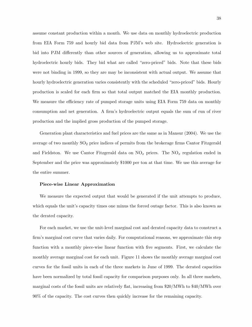
38

assume constant production within a month. We use data on monthly hydroelectric production

from EIA Form 759 and hourly bid data from PJM’s web site. Hydroelectric generation is

bid into PJM differently than other sources of generation, allowing us to approximate total

hydroelectric hourly bids. They bid what are called “zero-priced” bids. Note that these bids

were not binding in 1999, so they are may be inconsistent with actual output. We assume that

hourly hydroelectric generation varies consistently with the scheduled “zero-priced” bids. Hourly

production is scaled for each firm so that total output matched the EIA monthly production.

We measure the efficiency rate of pumped storage units using EIA Form 759 data on monthly

consumption and net generation. A firm’s hydroelectric output equals the sum of run of river

production and the implied gross production of the pumped storage.

Generation plant characteristics and fuel prices are the same as in Mansur (2004). We use the

average of two monthly SO2 price indices of permits from the brokerage firms Cantor Fitzgerald

and Fieldston. We use Cantor Fitzgerald data on NOx prices. The NOx regulation ended in

September and the price was approximately $1000 per ton at that time. We use this average for

the entire summer.

Piece-wise Linear Approximation

We measure the expected output that would be generated if the unit attempts to produce,

which equals the unit’s capacity times one minus the forced outage factor. This is also known as

the derated capacity.

For each market, we use the unit-level marginal cost and derated capacity data to construct a

firm’s marginal cost curve that varies daily. For computational reasons, we approximate this step

function with a monthly piece-wise linear function with five segments. First, we calculate the

monthly average marginal cost for each unit. Figure 11 shows the monthly average marginal cost

curves for the fossil units in each of the three markets in June of 1999. The derated capacities

have been normalized by total fossil capacity for comparison purposes only. In all three markets,

marginal costs of the fossil units are relatively flat, increasing from $20/MWh to $40/MWh over

90% of the capacity. The cost curves then quickly increase for the remaining capacity.

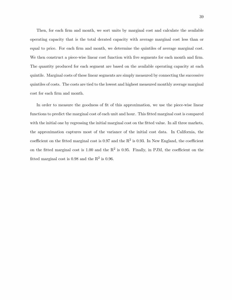
39

Then, for each firm and month, we sort units by marginal cost and calculate the available

operating capacity that is the total derated capacity with average marginal cost less than or

equal to price. For each firm and month, we determine the quintiles of average marginal cost.

We then construct a piece-wise linear cost function with five segments for each month and firm.

The quantity produced for each segment are based on the available operating capacity at each

quintile. Marginal costs of these linear segments are simply measured by connecting the successive

quintiles of costs. The costs are tied to the lowest and highest measured monthly average marginal

cost for each firm and month.

In order to measure the goodness of fit of this approximation, we use the piece-wise linear

functions to predict the marginal cost of each unit and hour. This fitted marginal cost is compared

with the initial one by regressing the initial marginal cost on the fitted value. In all three markets,

the approximation captures most of the variance of the initial cost data. In California, the

coefficient on the fitted marginal cost is 0.97 and the R2 is 0.93. In New England, the coefficient

on the fitted marginal cost is 1.00 and the R2 is 0.95. Finally, in PJM, the coefficient on the

fitted marginal cost is 0.98 and the R2 is 0.96.

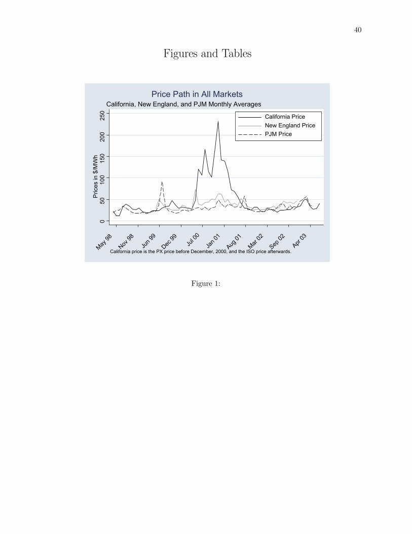
40

Figures and Tables

050

100

150

200

250

Pric

es in

$/M

Wh

May 98

Nov 98

Jun 9

9

Dec 99

Jul 0

0

Jan 0

1

Aug 01

Mar 02

Sep 02

Apr 03

California PriceNew England PricePJM Price

California price is the PX price before December, 2000, and the ISO price afterwards.

California, New England, and PJM Monthly AveragesPrice Path in All Markets

Figure 1:

41

0.00

1.00

2.00

3.00

Kern

el D

ensi

ty

0.40 0.60 0.80 1.00Ratio of Current Demand to Summer Peak Demand

MeanCalifornia 0.627New England 0.671PJM 0.635

Kernel Density of Demand by Market

Figure 2:

025

5075

100

Pric

es in

$/M

Wh

0.40 0.60 0.80 1.00Ratio of Current Demand to Summer Peak Demand

Actual PriceActual Price KernelCournot Price KernelCompetitive Price Kernel

We calculate nonparametric regressions using the k-Nearest Neighbor estimator.

Actual, Competitive, and Cournot Price KernelsPrices by Quantity Demanded in California

Figure 3:

42

025

050

075

010

00Pr

ices

in $

/MW

h

0.40 0.60 0.80 1.00Ratio of Current Demand to Summer Peak Demand

Actual PriceActual Price KernelCournot Price KernelCompetitive Price Kernel

We calculate nonparametric regressions using the k-Nearest Neighbor estimator.

Actual, Competitive, and Cournot Price KernelsPrices by Quantity Demanded in New England

Figure 4:

025

050

075

010

00P

rices

in $

/MW

h

0.40 0.60 0.80 1.00Ratio of Current Demand to Summer Peak Demand

Actual Price Actual Price KernelCournot Price Kernel Competitive Price Kernel

We calculate nonparametric regressions using the k-Nearest Neighbor estimator.

Actual, Competitive, and Cournot Price KernelsPrices by Quantity Demanded in PJM

Figure 5:

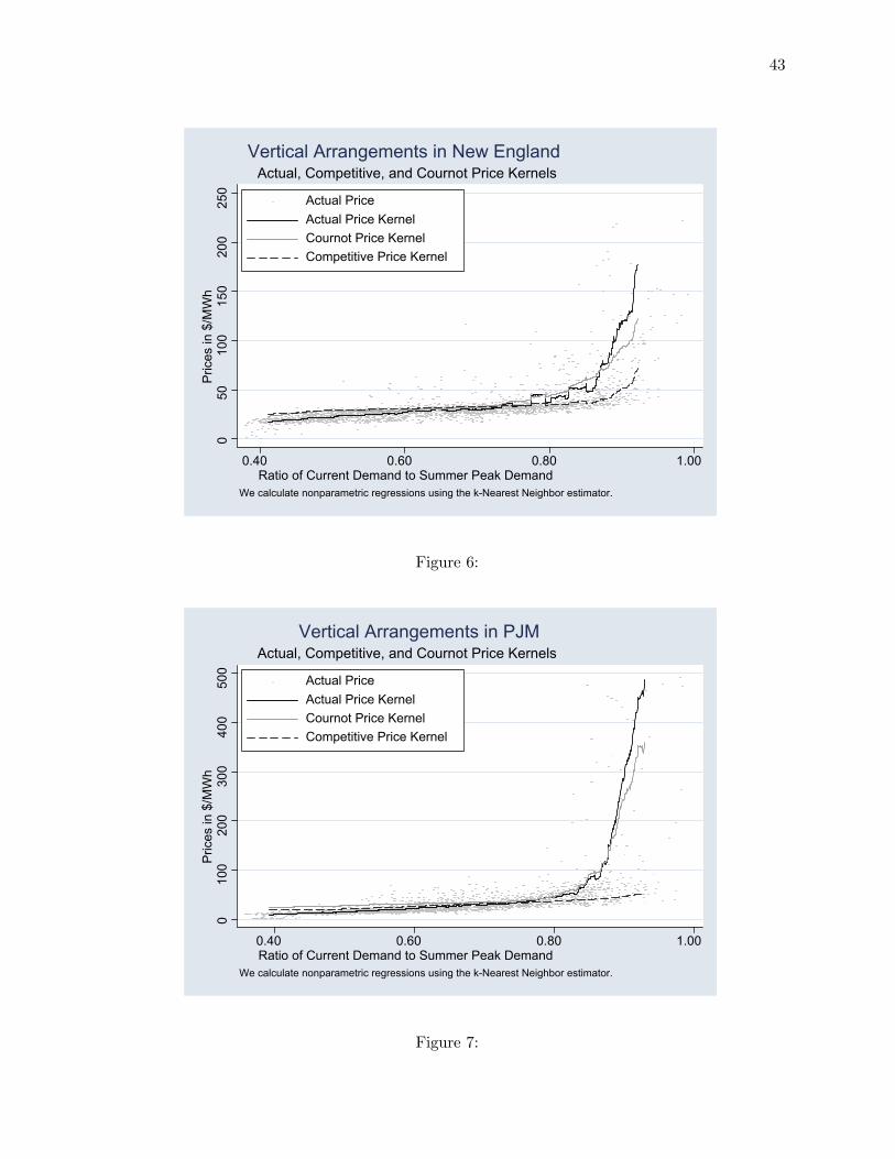
43

050

100

150

200

250

Pric

es in

$/M

Wh

0.40 0.60 0.80 1.00Ratio of Current Demand to Summer Peak Demand

Actual PriceActual Price KernelCournot Price KernelCompetitive Price Kernel

We calculate nonparametric regressions using the k-Nearest Neighbor estimator.

Actual, Competitive, and Cournot Price KernelsVertical Arrangements in New England

Figure 6:

010

020

030

040

050

0Pr

ices

in $

/MW

h

0.40 0.60 0.80 1.00Ratio of Current Demand to Summer Peak Demand

Actual PriceActual Price KernelCournot Price KernelCompetitive Price Kernel

We calculate nonparametric regressions using the k-Nearest Neighbor estimator.

Actual, Competitive, and Cournot Price KernelsVertical Arrangements in PJM

Figure 7:

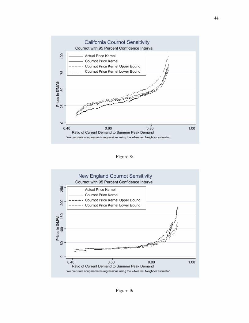
44

025

5075

100

Pric

es in

$/M

Wh

0.40 0.60 0.80 1.00Ratio of Current Demand to Summer Peak Demand

Actual Price KernelCournot Price KernelCournot Price Kernel Upper BoundCournot Price Kernel Lower Bound

We calculate nonparametric regressions using the k-Nearest Neighbor estimator.

Cournot with 95 Percent Confidence IntervalCalifornia Cournot Sensitivity

Figure 8:

050

100

150

200

250

Pric

es in

$/M

Wh

0.40 0.60 0.80 1.00Ratio of Current Demand to Summer Peak Demand

Actual Price KernelCournot Price KernelCournot Price Kernel Upper BoundCournot Price Kernel Lower Bound

We calculate nonparametric regressions using the k-Nearest Neighbor estimator.

Cournot with 95 Percent Confidence IntervalNew England Cournot Sensitivity

Figure 9:

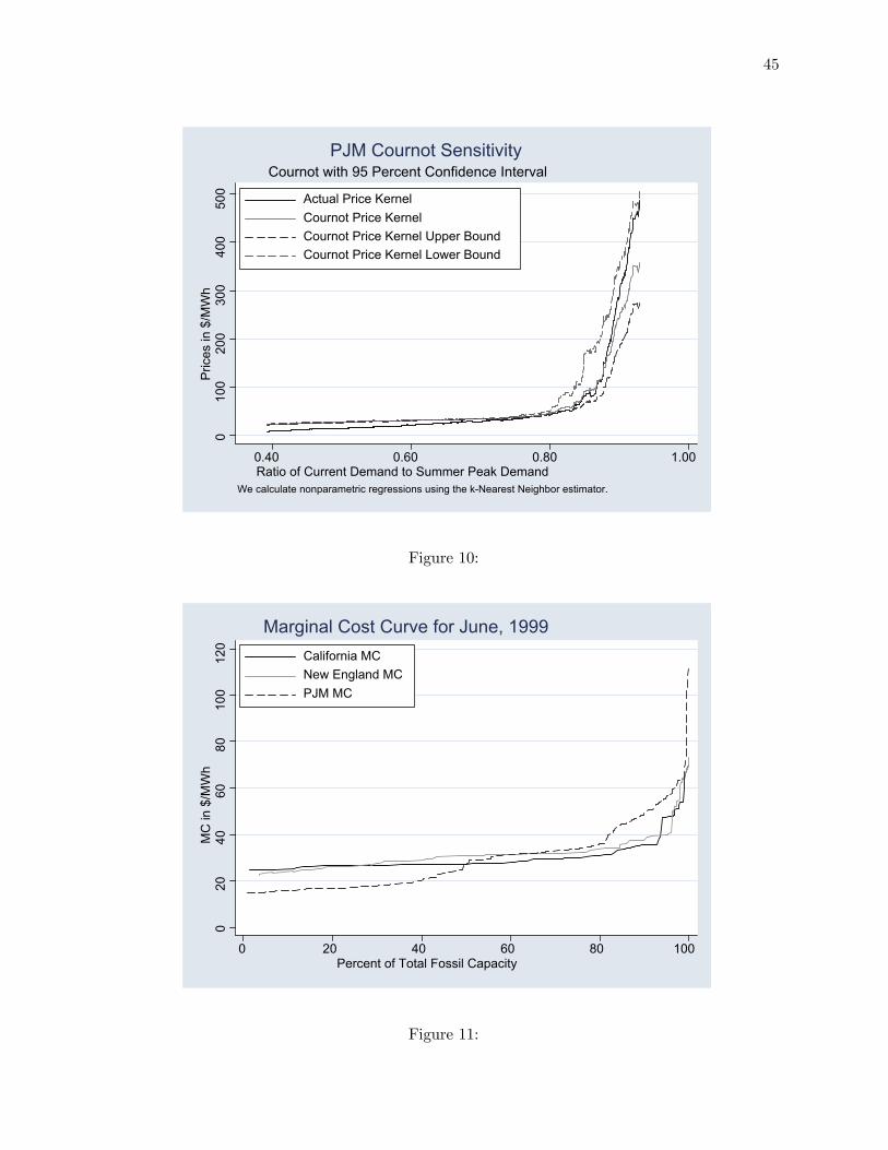
45

010

020

030

040

050

0Pr

ices

in $

/MW

h

0.40 0.60 0.80 1.00Ratio of Current Demand to Summer Peak Demand

Actual Price KernelCournot Price KernelCournot Price Kernel Upper BoundCournot Price Kernel Lower Bound

We calculate nonparametric regressions using the k-Nearest Neighbor estimator.

Cournot with 95 Percent Confidence IntervalPJM Cournot Sensitivity

Figure 10:

020

4060

8010

012

0M

C in

$/M

Wh

0 20 40 60 80 100Percent of Total Fossil Capacity

California MCNew England MCPJM MC

Marginal Cost Curve for June, 1999

Figure 11:

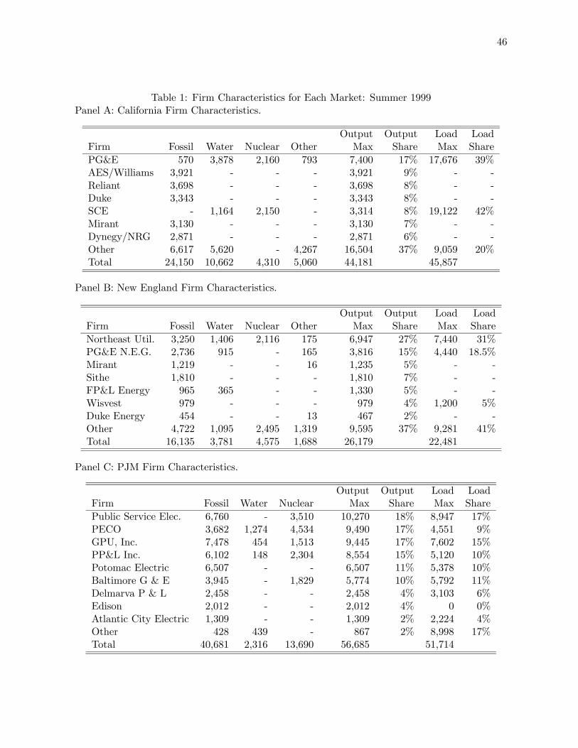
46

Table 1: Firm Characteristics for Each Market: Summer 1999Panel A: California Firm Characteristics.

Output Output Load LoadFirm Fossil Water Nuclear Other Max Share Max Share

PG&E 570 3,878 2,160 793 7,400 17% 17,676 39%AES/Williams 3,921 - - - 3,921 9% - -Reliant 3,698 - - - 3,698 8% - -Duke 3,343 - - - 3,343 8% - -SCE - 1,164 2,150 - 3,314 8% 19,122 42%Mirant 3,130 - - - 3,130 7% - -Dynegy/NRG 2,871 - - - 2,871 6% - -Other 6,617 5,620 - 4,267 16,504 37% 9,059 20%Total 24,150 10,662 4,310 5,060 44,181 45,857

Panel B: New England Firm Characteristics.

Output Output Load LoadFirm Fossil Water Nuclear Other Max Share Max Share

Northeast Util. 3,250 1,406 2,116 175 6,947 27% 7,440 31%PG&E N.E.G. 2,736 915 - 165 3,816 15% 4,440 18.5%Mirant 1,219 - - 16 1,235 5% - -Sithe 1,810 - - - 1,810 7% - -FP&L Energy 965 365 - - 1,330 5% - -Wisvest 979 - - - 979 4% 1,200 5%Duke Energy 454 - - 13 467 2% - -Other 4,722 1,095 2,495 1,319 9,595 37% 9,281 41%Total 16,135 3,781 4,575 1,688 26,179 22,481

Panel C: PJM Firm Characteristics.

Output Output Load LoadFirm Fossil Water Nuclear Max Share Max Share

Public Service Elec. 6,760 - 3,510 10,270 18% 8,947 17%PECO 3,682 1,274 4,534 9,490 17% 4,551 9%GPU, Inc. 7,478 454 1,513 9,445 17% 7,602 15%PP&L Inc. 6,102 148 2,304 8,554 15% 5,120 10%Potomac Electric 6,507 - - 6,507 11% 5,378 10%Baltimore G & E 3,945 - 1,829 5,774 10% 5,792 11%Delmarva P & L 2,458 - - 2,458 4% 3,103 6%Edison 2,012 - - 2,012 4% 0 0%Atlantic City Electric 1,309 - - 1,309 2% 2,224 4%Other 428 439 - 867 2% 8,998 17%Total 40,681 2,316 13,690 56,685 51,714

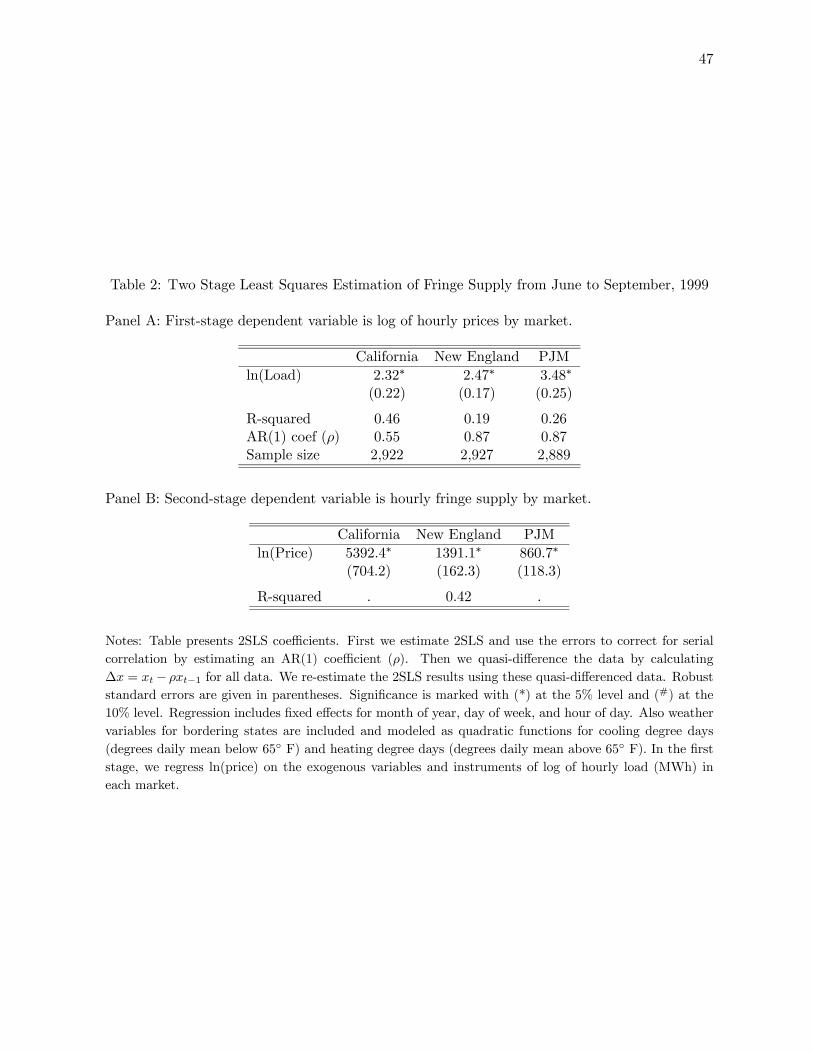
47

Table 2: Two Stage Least Squares Estimation of Fringe Supply from June to September, 1999

Panel A: First-stage dependent variable is log of hourly prices by market.

California New England PJM

ln(Load) 2.32∗ 2.47∗ 3.48∗

(0.22) (0.17) (0.25)

R-squared 0.46 0.19 0.26AR(1) coef (ρ) 0.55 0.87 0.87Sample size 2,922 2,927 2,889

Panel B: Second-stage dependent variable is hourly fringe supply by market.

California New England PJM

ln(Price) 5392.4∗ 1391.1∗ 860.7∗

(704.2) (162.3) (118.3)

R-squared . 0.42 .

Notes: Table presents 2SLS coefficients. First we estimate 2SLS and use the errors to correct for serial

correlation by estimating an AR(1) coefficient (ρ). Then we quasi-difference the data by calculating

∆x = xt− ρxt−1 for all data. We re-estimate the 2SLS results using these quasi-differenced data. Robuststandard errors are given in parentheses. Significance is marked with (*) at the 5% level and (#) at the

10% level. Regression includes fixed effects for month of year, day of week, and hour of day. Also weather

variables for bordering states are included and modeled as quadratic functions for cooling degree days

(degrees daily mean below 65◦ F) and heating degree days (degrees daily mean above 65◦ F). In the firststage, we regress ln(price) on the exogenous variables and instruments of log of hourly load (MWh) in

each market.

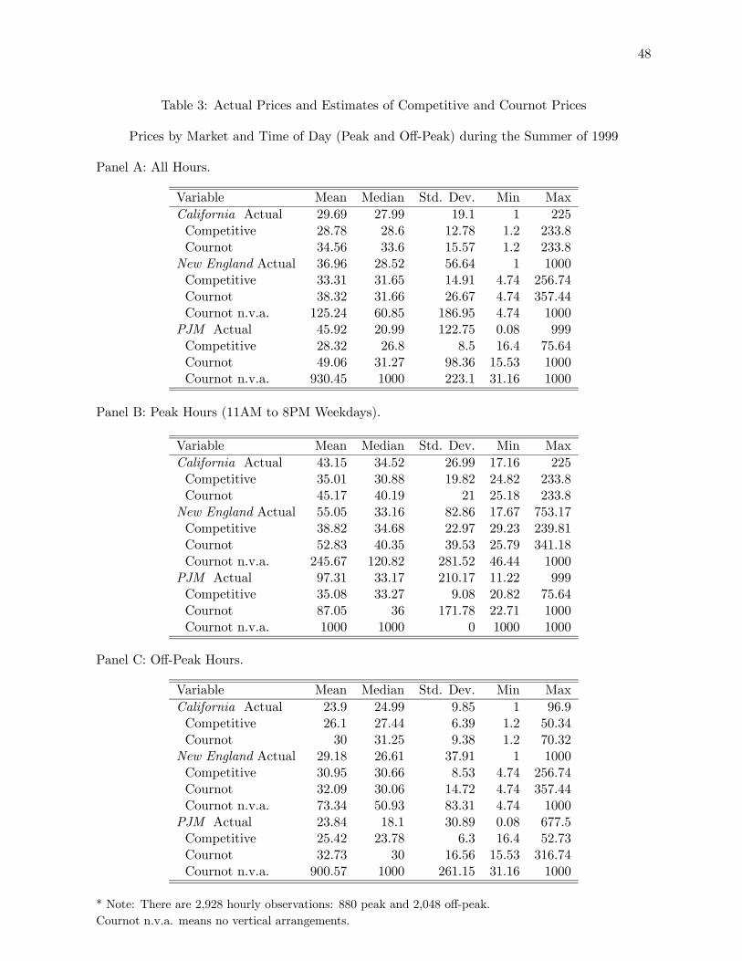
48

Table 3: Actual Prices and Estimates of Competitive and Cournot Prices

Prices by Market and Time of Day (Peak and Off-Peak) during the Summer of 1999

Panel A: All Hours.

Variable Mean Median Std. Dev. Min Max

California Actual 29.69 27.99 19.1 1 225Competitive 28.78 28.6 12.78 1.2 233.8Cournot 34.56 33.6 15.57 1.2 233.8New England Actual 36.96 28.52 56.64 1 1000Competitive 33.31 31.65 14.91 4.74 256.74Cournot 38.32 31.66 26.67 4.74 357.44Cournot n.v.a. 125.24 60.85 186.95 4.74 1000PJM Actual 45.92 20.99 122.75 0.08 999Competitive 28.32 26.8 8.5 16.4 75.64Cournot 49.06 31.27 98.36 15.53 1000Cournot n.v.a. 930.45 1000 223.1 31.16 1000

Panel B: Peak Hours (11AM to 8PM Weekdays).

Variable Mean Median Std. Dev. Min Max

California Actual 43.15 34.52 26.99 17.16 225Competitive 35.01 30.88 19.82 24.82 233.8Cournot 45.17 40.19 21 25.18 233.8New England Actual 55.05 33.16 82.86 17.67 753.17Competitive 38.82 34.68 22.97 29.23 239.81Cournot 52.83 40.35 39.53 25.79 341.18Cournot n.v.a. 245.67 120.82 281.52 46.44 1000PJM Actual 97.31 33.17 210.17 11.22 999Competitive 35.08 33.27 9.08 20.82 75.64Cournot 87.05 36 171.78 22.71 1000Cournot n.v.a. 1000 1000 0 1000 1000

Panel C: Off-Peak Hours.

Variable Mean Median Std. Dev. Min Max

California Actual 23.9 24.99 9.85 1 96.9Competitive 26.1 27.44 6.39 1.2 50.34Cournot 30 31.25 9.38 1.2 70.32New England Actual 29.18 26.61 37.91 1 1000Competitive 30.95 30.66 8.53 4.74 256.74Cournot 32.09 30.06 14.72 4.74 357.44Cournot n.v.a. 73.34 50.93 83.31 4.74 1000PJM Actual 23.84 18.1 30.89 0.08 677.5Competitive 25.42 23.78 6.3 16.4 52.73Cournot 32.73 30 16.56 15.53 316.74Cournot n.v.a. 900.57 1000 261.15 31.16 1000

* Note: There are 2,928 hourly observations: 880 peak and 2,048 off-peak.

Cournot n.v.a. means no vertical arrangements.