Graph

Version 4.4

Copyright © 2012 Ivan Johansen

ii

Table of ContentsWhat is Graph? ......................................................................................................................... 1How to use Graph ..................................................................................................................... 2Installation and startup ............................................................................................................... 3Frequently Asked Questions ........................................................................................................ 5OLE server/client ...................................................................................................................... 7List of menu items .................................................................................................................... 8Error messages ........................................................................................................................ 12Functions ................................................................................................................................ 15

List of functions .............................................................................................................. 15Constants ........................................................................................................................ 19

rand constant ........................................................................................................... 19Trigonometric .................................................................................................................. 19

sin function ............................................................................................................. 19cos function ............................................................................................................ 19tan function ............................................................................................................ 20asin function ........................................................................................................... 20acos function ........................................................................................................... 20atan function ........................................................................................................... 20sec function ............................................................................................................ 21csc function ............................................................................................................ 21cot function ............................................................................................................ 21asec function ........................................................................................................... 22acsc function ........................................................................................................... 22acot function ........................................................................................................... 22

Hyperbolic ...................................................................................................................... 22sinh function ........................................................................................................... 22cosh function .......................................................................................................... 23tanh function ........................................................................................................... 23asinh function .......................................................................................................... 23acosh function ......................................................................................................... 23atanh function ......................................................................................................... 24csch function ........................................................................................................... 24sech function ........................................................................................................... 24coth function ........................................................................................................... 24acsch function ......................................................................................................... 25asech function ......................................................................................................... 25acoth function ......................................................................................................... 25

Power and logarithm ........................................................................................................ 25sqr function ............................................................................................................ 25exp function ............................................................................................................ 26sqrt function ............................................................................................................ 26root function ........................................................................................................... 26ln function .............................................................................................................. 26log function ............................................................................................................ 27logb function ........................................................................................................... 27

Complex ......................................................................................................................... 27abs function ............................................................................................................ 27arg function ............................................................................................................ 28conj function ........................................................................................................... 28re function .............................................................................................................. 28im function ............................................................................................................. 28

Rounding ........................................................................................................................ 29trunc function .......................................................................................................... 29fract function .......................................................................................................... 29ceil function ............................................................................................................ 29

Graph

iii

floor function .......................................................................................................... 29round function ......................................................................................................... 30

Piecewise ........................................................................................................................ 30sign function ........................................................................................................... 30u function ............................................................................................................... 30min function ........................................................................................................... 30max function ........................................................................................................... 31range function ......................................................................................................... 31if function .............................................................................................................. 31

Special ........................................................................................................................... 31integrate function ..................................................................................................... 31sum function ........................................................................................................... 32product function ...................................................................................................... 32fact function ............................................................................................................ 32gamma function ....................................................................................................... 33beta function ........................................................................................................... 33W function ............................................................................................................. 33zeta function ........................................................................................................... 34mod function ........................................................................................................... 34dnorm function ........................................................................................................ 34

Dialogs .................................................................................................................................. 36Edit axes ........................................................................................................................ 36Options .......................................................................................................................... 38Insert function ................................................................................................................. 39Insert tangent/normal ........................................................................................................ 41Insert shading .................................................................................................................. 42Insert point series ............................................................................................................. 44Insert trendline ................................................................................................................ 46Insert label ...................................................................................................................... 48Insert relation .................................................................................................................. 49Insert f'(x) ...................................................................................................................... 50Custom functions/constants ................................................................................................ 51Evaluate ......................................................................................................................... 51Table ............................................................................................................................. 53Animate ......................................................................................................................... 54Save as image ................................................................................................................. 55Import point series ........................................................................................................... 55

Plugins ................................................................................................................................... 57Acknowledgements .................................................................................................................. 58Glossary ................................................................................................................................. 61

1

What is Graph?Graph is a program designed to draw graphs of mathematical functions in a coordinate system and similarthings. The program is a standard Windows program with menus and dialogs. The program is capable ofdrawing standard functions, parametric functions, polar functions, tangents, point series, shadings andrelations. It is also possible to evaluate a function for a given point, trace a graph with the mouse and muchmore. For more information on using the program see How to use Graph.

Graph is free software; you can redistribute it and/or modify it under the terms of the GNU General PublicLicense [http://www.gnu.org/licenses/gpl.html]. Newest version of the program as well as the source codemay be downloaded from http://www.padowan.dk.

Graph has been tested under Windows 2000, Windows XP, Windows Vista and Windows 7, but there maystill be bugs left. If you need help using Graph or have suggestions for future improvements, please use theGraph support forum [http://www.padowan.dk/forum].

When you send a bug report, please write the following:

• Which version are you using? This is shown in the Help → About Graph dialog box. You should checkthat you are using the newest version as the bug may have been fixed already.

• Explain what happens and what you expected to happen.

• Explain carefully how I can reproduce the bug. If I can't see what you see, it is very difficult for me tosolve the problem.

2

How to use GraphWhen the program starts, you will see the main window shown below. This window shows the graphing areato the right with the coordinate system where the graphs you insert will be shown. You can use the menu orthe buttons on the toolbar to show different dialog boxes to insert a function, edit functions, delete functionsetc. You can find a description of all the menu items.

The toolbar may be customized by right clicking on the bar and selecting Customize toolbar... from thepopup menu. You can then customize the toolbar by dragging commands to and from the bar. The status barat the bottom of the window shows tooltips or other information to the left and the coordinates located at themouse pointer to the right.

You can add new elements to the coordinate system from the Function menu. For example if you want to add

a new function you use the menu item Function → Insert function...

The function list to the left shows a list of functions, tangents, point series, shadings and relations you haveadded. If you want to manipulate anything in the list, just select it and use the Function menu. You can alsoright click on an item in the list to get the context menu with available commands. An item may be edited bydouble clicking on it.

The Calc menu contains commands to make calculations on functions, for example evaluations at specificcoordinates or given intervals.

3

Installation and startupInstallation

Graph is usually distributed as an installation program named SetupGraph-x.y.exe, where x.y is the versionnumber. To install, just execute the file and follow the instructions. The installation will install the followingfiles in the selected directory and subdirectories:

File(s) Description

Graph.exe The program file.

PDFlib.dll Library used to create PDF files.

Thumbnails.dll Shell extension for showing thumbnails of grf-files in Explorer.

Locale\*.mo Translations of the program.

Help\*.chm Help files in different languages.

Plugins\*.py Some examples of plugins. Custom plugins can be placed here too.

Lib\*.py Library files used by plugins.

Examples\*.grf Some examples that can be opened in Graph.

The installation will create a shortcut in the Start menu, which may be used to start the program. During theinstallation you select the preferred language. This can later be changed from the Options dialog.

If an older version of the program is already installed, the installation suggests you install in the samedirectory. You can just install over the old version. There is no need to uninstall the old version first, butmake sure the old version is not running while installing.

The Graph Setup can take the parameters specified in the table below. These are especially useful when youwant to automate the installation.

Parameter Description

/SILENT Instructs the Setup to be silent, which means that the wizard and the backgroundwindow are not displayed but the installation progress window is. Everything elseis normal so for example error messages during installation are displayed. If arestart is necessary, a Reboot now? message box is displayed.

/VERYSILENT Instructs the Setup to be very silent. This is the same as silent with the additionthat the installation progress window is not displayed either. If a restart isnecessary, the Setup will reboot without asking.

/NORESTART Instructs Setup not to reboot even if it's necessary.

/LANG=language Specifies the language to use. language specifies the English name of thelanguage. When a valid /LANG parameter is used, the Select language dialogwill be suppressed.

/DIR=x:\dirname Overrides the default directory name displayed on the Select destinationlocation wizard page. A fully qualified pathname must be specified.

UninstallationUninstallation is done from Add/Remove Programs in the Control Panel. Just select Graph and click on theChange/Remove button. This will remove all traces of the program. If files were added to the installationdirectory after the installation, you will be asked if you want to delete them. Make sure Graph is not runningwhile uninstalling.

Installation and startup

4

StartupUsually Graph is started from the link in the Start menu. A .grf file can be passed as parameter, in which caseGraph will open the specified file. In addition to this the parameters in the table below can be passed to Graphon the command line.

Parameter Description

/SI=file Used to save an opened .grf file as an image file. The file type can be any of theimage formats supported by Graph.

/WIDTH=width Used in combination with /SI to specify the width in pixels of the image to besaved.

/HEIGHT=height Used in combination with /SI to specify the height in pixels of the image to besaved.

5

Frequently Asked QuestionsQ: What are the system requirements of Graph?

A: Graph requires Microsoft Windows 2000 or newer. It has been tested under Windows 2000, WindowsXP, Windows Vista and Windows 7.

Q: Will Graph run under Linux?

A: Graph is a native Windows application and not tested under Linux, but several users have informed methat Graph runs without problems under Linux with Wine.

Q: Will Graph run on a Mac?

A: As with the above, you cannot run Graph directly on a Mac. However a bundle of Graph with Wine isavailable from the website [http://www.padowan.dk/graph-on-mac/].

Q: When will the next version be released?

A: When it is ready.

Q: How can I move the coordinate system?

A: When you hold down the Ctrl key you can use the arrow keys to move the coordinate system. You can

also use Zoom → Move system and drag the coordinate system around with the mouse.

Q: How can I easily zoom in and out?

A: When you hold down the Ctrl key you can use the + and - keys to zoom in and out. The scroll wheelon the mouse can be used for zooming at the position of the mouse pointer. When you move the scrollwheel up the program will zoom into the coordinate system and center the graphing area at the positionof the mouse pointer. When you move the scroll wheel down the program zooms out.

Q: How do I save default settings?

A: Set the desired default settings in the Edit axes dialog, and put a mark in Save as default beforepressing the OK button. Next time you create a new coordinate system, the saved default settings will beused.

Q: Can I make the program remember the size and position of the window?

A: When you select Save workspace on exit in the Options dialog. Graph will save the position and sizeof the main window when the program quits. The next time the program starts the same size and positionis used.

Q: Why does the program not accept a comma as decimals separator?

A: I know a lot of countries use comma to separate the decimal part from the integer part, but Graph usescomma for separating function arguments. The program always uses a period to separate decimals fromthe integer value, no matter your local settings.

Q: How do I plot a vertical line?

A: A vertical line can be drawn as a parametric function. Select Parametric function as Functiontype when adding the function. You can then add the vertical line at x=5 as x(t)=5, y(t)=t.Alternatively you can add x=5 as a relation.

Q: How do I plot a function x=f(y)?

A: To draw a function with y as the independent variable, you need to use a parametric function. SelectParametric function as Function type when adding the function. If you want to draw the function

Frequently Asked Questions

6

x=sin(y), you can now enter the function as x(t)=sin(t), y(t)=t. Alternatively you can draw itas a relation where you can enter x=sin(y) directly.

Q: How do I plot a circle?

A: You need to use a parametric function to draw a circle. When inserting the function, selectParametric function as Function type. You can now add a circle with radius 5 and center in (2,3) as

x(t)=5cos(t)+2, y(t)=5sin(t)+3. You may need to use Zoom → Square to make the axesequally scaled. Else the circle may look like an ellipse. A circle can also be added as a polar function,but only with center in (0,0). A circle with radius 5 may be added as the polar function r(t)=5.Alternatively you can use a relation and add the circle as (x-2)^2+(y-3)^2=5^2.

Q: Why do circles look like ellipses?

A: That is probably because the axes are not equally scaled. You can either change the size of the window

until the axes scales equally or select Zoom → Square in the menu to change the y-axis to scale equalto the x-axis.

Q: How do I calculate the area between two functions?

A: If you want to find the area between two functions f1(x)=3x and f2(x)=x^2, the easiest way is to createa new function that is the difference between the two functions: f(x)=f1(x)-f2(x)=3x-x^2. You can then

use Calc → Integrate to calculate the area for a given interval.

Q: How do I plot the inverse of any given function?

A: You can use a parametric function for this. If you want to plot the inverse of f(x)=x2-2x, you can insert itas the parametric function x(t)=t^2-2t, y(t)=t.

Q: How can I draw the negative part of f(x)=sqrt(x+2) ?

A: For each value x, f(x) will evaluate to at most one value. f(x)=sqrt(x+2) will therefore only havepositive values of f(x). To plot it for negative f(x) too, you will have to create two separate functions:f(x)=sqrt(x+2) and f(x)=-sqrt(x+2). Alternatively you can plot it as the relation: y^2=x+2.

Q: How do I plot a complex function like f(t)=e^(i*t)?

A: You probably want to show the real part on the x-axis and the imaginary part on the y-axis. In that caseyou can draw the function as the parametric function x(t)=re(e^(i*t)), y(t)=im(e^(i*t)).Notice that Calculate with complex numbers must be enabled in the Edit axes dialog.

Q: How can I make Graph plot functions with vertical asymptotes correctly?

A: Functions like f(x)=tan(x) with vertical asymptotes may not always be shown correctly. As defaultGraph will evaluate the function for each pixel on the x-axis. But if the graph has a steep slope that goesagainst infinite and back between two pixels, Graph will not notice it. To plot the function correctly youcan tell Graph how many evaluations to perform. This may be entered in the Steps field in the Insertfunction dialog. A number around 100000 will usually show the function correctly.

Q: How to create a PDF file from Graph?

A: You can choose to save as PDF in the Save as image dialog.

Q: Why will the program not start under Windows 95?

A: Graph no longer supports Windows 95. The last version to run under Windows 95 was Graph 4.2.

7

OLE server/clientOLE server

Graph has been implemented as an OLE (Object Linking and Embedding) server, which means that Graphobjects can be placed (embedded) into an OLE client. Many applications can work as OLE clients, forexample Microsoft Word.

You can use Edit → Copy image in Graph to copy the current content to the clipboard. Afterwards you canselect Paste in Word (or similar in another OLE client) to insert the Graph object from the clipboard. Whenyou double click on the object a new instance of Graph will start where you can edit the object. If you don't

want to paste the data as a Graph object into Word, you can use Paste → Paste Special... in Word to pasteas a picture instead.

You may create a new Graph object in Word by choosing Object in the toolbar and selecting Graph systemas Object type. The same dialog can be used to create an embedded Graph object from an existing grf-file.If you select Link to file, you will get a linked object instead of an embedded object. This way all changes tothe object will be reflected in the original grf-file. If the grf-file is not available you will not be able to edit theobject, but you can still see the image in Word.

To edit a Graph object you must have Graph installed on the system. If Graph is not installed you will still beable to see the image but not edit it.

OLE clientGraph can work as an OLE client as a text label in Graph is an OLE container. This means that you can pasteimages and OLE objects into the editor used to add labels. As in any other OLE container you can edit theobject by double clicking on it. From the context menu you can use Insert object... to create a new OLEobject in the label. The same dialog can be used to create an object from a file. You can for example insert animage file this way. To edit an OLE object the server must be installed on the system, else you will only beable to see object but not edit it.

8

List of menu itemsThe following is a list of all the menu items in the program:

File → New (Ctrl+N)Use this to create a new coordinate system for drawing graphs in.

File → Open... (Ctrl+O)Reads an earlier saved coordinate system from a .grf file.

File → Save (Ctrl+S)Saves the coordinate system to a file.

File → Save as...Saves the coordinate system to a file with a new name.

File → Save as image... (Ctrl+B) Saves the shown coordinate system as an image.

File → Import → Graph file...Imports the contents of another Graph file into the current coordinate system.

File → Import → Point series... Imports one or several point series from a tab, comma or semicolon separated data file. The first columnshall contain the x-coordinates. The following columns shall contain the y-coordinates. Graph will createas many point series as there are columns with y-coordinates in the file. There is no limit to the numberof point series possible in the data file as long as they share the same x-coordinates.

File → Print... (Ctrl+P)Sends the coordinate system and graphs to a printer.

File → Exit (Alt+F4)Quits the program. You may be asked to save the file.

Edit → Undo (Ctrl+Z)Use this to undo the last thing you did. You can choose how many undo steps that are saved in theOptions dialog.

Edit → Redo (Ctrl+Y)

Use this to redo the last thing undone. This is only available after you have selected Edit → Undo.

Edit → Cut (Ctrl+X)This will copy the selected graph element to the clipboard. The element will be deleted afterwards.

Edit → Copy (Ctrl+C)This will copy the selected graph element to the clipboard.

Edit → Paste (Ctrl+V)This will paste an earlier copied graph element from the clipboard into the coordinate system.

Edit → Copy image (Ctrl+I)Copies the shown coordinate system to the clipboard as an image. You can then paste it into anotherprogram, i.e. Microsoft Word.

Edit → Axes... (Ctrl+A) Edit specifications for the axes, e.g. scale, colors, legend placement, etc.

List of menu items

9

Edit → Options... This will change global settings for Graph, e.g. association of .grf files, showing of tooltips, maximumnumber of undo stored undo steps, etc.

Function → Insert function... (Ins) Inserts a function into the coordinate system. Functions may be added with different width and color, andyou can choose to only show the graph in a specified interval, and specify other settings too.

Function → Insert tangent... (F2) Use this dialog to add a tangent to an already shown function at a user-specified point. The tangent willbe added to the function selected in the function list.

Function → Insert shading... (F3) This menu item is used to add a shading to the selected function. You may choose between differentstyles of shading and different colors. The shading may be added above the function, below the function,between the function and the x-axis, between the function and the y-axis, inside the function or betweentwo functions.

Function → Insert f'(x)... (F7) This dialog is used to add the first derivative to the selected function.

Function → Insert point series... (F4) Inserts a new point series into the coordinate system. An infinite number of points defined by their x- andy-coordinates may be added. It is possible to choose color, size, and style of the point series.

Function → Insert trendline... (Ctrl+T) Inserts a trendline as the curve of best fit for the selected point series. You may choose between differentkinds of functions for the trendline.

Function → Insert relation... (F6) This inserts an equation or inequality into the coordinate system. Equations and inequalities are used toexpress relations between x- and y-coordinates with the same operators etc. as for graphs of functions.Relations may be added with different shading styles and colors.

Function → Insert label... (F8) This will show a dialog, which may be used to create a formatted text label. The label will always becreated at the center of the graphing area but can afterwards be dragged to another place with the mouse.

Function → Edit... (Enter)This will show a dialog where you can change the selected graph element in the function list.

Function → Delete (Del)This will delete the selected graph element in the function list.

Function → Custom functions... (Ctrl+F) This shows a dialog used to create custom functions and constants in addition to the built-in ones.

Zoom → In (Ctrl++)This will zoom in at the center of the graphing area, so you will see 81% of the previous graphing area. Ifyou hold down Shift it will zoom in more, so you see 25% of the previous graphing area.

Zoom → Out (Ctrl+-)This will zoom out so you see 1.23 times as much as on the previous graphing area. If you hold downShift it will zoom out more, so you see 4 times the previous graphing area.

List of menu items

10

Zoom → Window (Ctrl+W)Hold down the left mouse button while you select the area you want to fill the whole graphing area.Right click or press Esc to cancel the command.

Zoom → Square (Ctrl+Q)This changes the y-axis to the same scale as the x-axis. It will make a circle look correctly instead ofshowing as an ellipse. The axes will stay equally scaled until disabled again.

Zoom → Standard (Ctrl+D)Returns the axes settings to the same default settings used when creating a new coordinate system.

Zoom → Move system (Ctrl+M)When selected the mouse pointer changes to a hand. You may now use the mouse to drag the coordinatesystem around. Select the menu item again, right click or press Esc to return to normal mode. As analternative to this menu item, you may hold down the Shift key and drag the coordinate system around.

Zoom → FitThis will change the axes settings to show all parts of the selected graph element.

Zoom → Fit allThis will change the axes settings to show all parts of all the elements in the function list.

Calc → Length of path Calculates the distance along the path between two points on the selected graph.

Calc → Integrate Calculates the definite integral for a specified domain range. This is the same as the signed area betweenthe graph and the x-axis.

Calc → Evaluate (Ctrl+E) This will evaluate the selected function for a given value. For standard functions f(x), f'(x) and f''(x) areevaluated. For parametric functions x(t), y(t), dx/dt, dy/dt and dy/dx are evaluated. For polar functionsr(t), x(t), y(t), dr/dt and dy/dt are evaluated.

Calc → Table... This dialog fills a table with a user-specified range of values and the result of evaluating the selectedfunction for the values.

Calc → Animate... This dialog allows you to create an animation from the data in the coordinate system by changing anexisting custom constant. This makes it easy to see what happens when the constant changes. Theanimation may be saved to a disk file.

PluginsThis is a common place for plugins to put menu items that activates the plugin. The menu will not beshown if there are no plugins or the plugin system is not available.

Help → Contents and index (F1)Shows the contents and index of the help file.

Help → List of functions (Ctrl+F1)Shows a list of functions and constants that may be used for plotting graphs.

Help → Frequently Asked QuestionsThis will show a list of frequently asked questions and their answers.

List of menu items

11

Help → Tip of the dayThis will show some tips about using Graph in a more optimal way, and certain features of Graph youmay not know about.

Help → Internet → Graph web siteShows the web site for Graph in your default web browser.

Help → Internet → SupportShows the support forum for Graph in your default web browser.

Help → Internet → DonateShows the web page that allows you to donate to the Graph project to support its development.

Help → Internet → Check for updateThis will check if a new version of Graph is available. If there is a new version, you will be asked if youwant to visit the web site of Graph to download the new version.

Help → About Graph (Alt+F1)Shows version number, copyright and license information for Graph.

ShortcutsShift+Drag

This allows you to move the coordinate system around. It is basically the same as selecting Zoom →Move system in the menu.

Scroll wheelYou can use the scroll wheel on the mouse to zoom in and out at the position of the cursor in thegraphing area.

Ctrl+ArrowHold down Ctrl while you use the arrow keys to move the view around in small step. If you also holddown Shift you can move in larger steps.

Ctrl+HomeThis zooms in on the x-axis in small steps. If you also hold down Shift you can zoom in larger steps.

Ctrl+EndThis zooms out on the x-axis in small steps. If you also hold down Shift you can zoom in larger steps.

Ctrl+PgUpThis zooms in on the y-axis in small steps. If you also hold down Shift you can zoom in larger steps.

Ctrl+PgDnThis zooms out on the y-axis in small steps. If you also hold down Shift you can zoom in larger steps.

12

Error messagesError 01: An error occurred while evaluating power function.

This error occurs when a number raised to the power of another number resulted in an error. For example(-4)^(-5.1) gives an error, because a negative number cannot be raised to a negative non integer numberwhen calculating with real numbers.

Error 02: Tangent to pi/2+n*pi (90°+n180° in degrees) is undefined.

tan(x) is undefined for x= π/2+πp = 90°+p180°, where p is an integer.

Error 03: Fact can only be calculated for positive integers.fact(x), which calculates the factorial number of x, is only defined for positive integers of x.

Error 04: Cannot take logarithm to number equal or less than zero.

The logarithmic functions ln(x) and log(x) are undefined for x≤0, when the calculation is done for realnumbers. When the calculations are done with complex numbers, x is only undefined at 0.

Error 05: sqrt is undefined for negative numbers.sqrt(x) is undefined for x<0, when the calculations are done for real numbers. sqrt(x) is defined for allnumbers, when the calculations are done with complex numbers.

Error 06: A part of the evaluation gave a number with an imaginary part.This error may occur when calculations are done with real numbers. If a part of the calculation resulted ina number with an imaginary part, the calculation cannot continue. An example of this is: sin(x+i)

Error 07: Division by zero.The program tried to divide by zero when calculating. A function is undefined for values where adivision by zero is needed. For example the function f(x)=1/x is undefined at x=0.

Error 08: Inverse trigonometric function out of range [-1;1]The inverse trigonometric functions asin(x) and acos(x) are only defined in the range [-1;1], and theyare not defined for any numbers with an imaginary part. The function atan(x) is defined for all numberswithout an imaginary part. This error may also happen if you are trying to take arg(0).

Error 09: The function is not defined for this value.This error may occur for functions that are not defined for a specific point. This is for example the casefor sign(x) and u(x) at x=0.

Error 10: atanh evaluated at undefined value.Inverse hyperbolic tangent atanh(x) is undefined at x=1 and x=-1, and not defined outside the intervalx=]-1;1[ when calculating with real numbers only.

Error 11: acosh evaluated at undefined value.

Inverse hyperbolic cosine acosh(x) is only defined for x≥1 when using real numbers. acosh(x) is definedfor all numbers when calculating with complex numbers.

Error 12: arg(0) is undefined.The argument of zero is undefined because 0 does not have an angle.

Error 13: Evaluation failed.This error occurs when a more complicated function like W(z) is evaluated, and the evaluation failed tofind an accurate result.

Error 14: Argument produced a function result with total loss of precision.An argument to a function call produced a result with total loss of significant digits, such as sin(1E70)which gives an arbitrary number in the range [-1;1].

Error messages

13

Error 15: The custom function/constant '%s' was not found or has the wrong number of arguments.A custom function or constant no longer exists. You can either define it again or remove all uses of thesymbol. This may also happen if a custom constant has been changed to a function or vice versa, or if thenumber of arguments to a custom function has been changed.

Error 16: Too many recursive callsToo many recursive calls have been executed. This is most likely caused by a function that calls itselfrecursively an infinite number of times, for example foo(x)=2*foo(x). The error may also occur if youjust call too many functions recursively.

Error 17: Overflow: A function returned a value too large to handle.A function call resulted in value too large to handle. This for example happens if you try to evaluatesinh(20000)

Error 18: A plugin function failed.A custom function in a Python plugin did not return a result. The Python interpreter window may showmore detailed information.

Error 50: Unexpected operator. Operator %s cannot be placed hereAn operator +, -, *, / or ^ was misplaced. This can happen if you try entering the function f(x)=^2, and itusually means that you forgot something in front of the operator.

Error 55: Right bracket missing.A right bracket is missing. Make sure you have the same number of left and right brackets.

Error 56: Invalid number of arguments supplied for the function '%s'You passed a wrong number of arguments to the specified function. Check the List of functions to findthe required number of arguments the function needs. This error may occur if you for example writesin(x,3).

Error 57: Comparison operator misplaced.Only two comparison operators in sequence are allowed. For example "sin(x) < y < cos(x)" is okay while"sin(x) < x < y < cos(x)" is invalid because there are three <-operators in sequence.

Error 58: Invalid number found. Use the format: -5.475E-8Something that looked like a number but wasn't has been found. For example this is an invalid number:4.5E. A number should be on the form nnn.fffEeee where nnn is the whole number part that may benegative. fff is the fraction part that is separated from the integer part with a dot '.'. The fraction partis optional, but either the integer part or the fraction part must be there. E is the exponent separatorand must be an 'E' in upper case. eee is the exponent optionally preceded by '-'. The exponent is onlyneeded if the E is there. Notice that 5E8 is the same as 5*10^8. Here are some examples of numbers:-5.475E-8, -0.55, .75, 23E4

Error 59: String is empty. You need to enter a formula.You didn't enter anything in the box. This is not allowed. You need to enter an expression.

Error 60: Comma is not allowed here. Use dot as decimal separator.Commas may not be used as decimal separator. You have to use a '.' to separate the fraction from theinteger part.

Error 61: Unexpected right bracket.A right bracket was found unexpectedly. Make sure the number of left and right brackets match.

Error 63: Number, constant or function expected.A factor, which may be a number, constant, variable or function, was expected.

Error 64: Parameter after constant or variable not allowed.Brackets may not be placed after a constant or variable. For example this is invalid: f(x)=x(5). Usef(x)=x*5 instead.

Error 65: Expression expected.An expression was expected. This may happen if you have empty brackets: f(x)=sin()

Error messages

14

Error 66: Unknown variable, function or constant: %sYou entered something that looks like a variable, function or constant but is unknown. Note that "x5" isnot the same as "x*5".

Error 67: Unknown character: %sAn unknown character was found.

Error 68: The end of the expression was unexpected.The end of the expression was found unexpectedly.

Error 70: Error parsing expressionAn error happened while parsing the function text. The string is not a valid function.

Error 71: A calculation resulted in an overflow.An overflow occurred under the calculation. This may happen when the numbers get too big.

Error 73: An invalid value was used in the calculation.An invalid value was used as data for the calculation.

Error 74: Not enough points for calculation.Not enough data points were provided to calculate the trendline. A polynomial needs at least one morepoint than the degree of the polynomial. A polynomial of third degree needs at least 4 points. All otherfunctions need at least two points.

Error 75: Illegal name %s for user defined function or constant.Names for user defined functions and constants must start with a letter and only contain letters anddecimal digits. You cannot use names that are already used by built-in functions and constants.

Error 76: Cannot differentiate recursive function.It is not possible to differentiate a recursive function because the resulting function will be infinitelylarge.

Error 79: Function %s cannot be differentiated.The function cannot be differentiated, because some part of the function does not have a first derivative.This is for example the case for arg(x), conj(x), re(x) and im(x).

Error 86: Not further specified error occurred under calculation.An error occurred while calculating. The exact cause is unknown. If you get this error, you may tryto contact the programmer with a description of how to reproduce the error. Then he might be able toimprove the error message or prevent the error from occurring.

Error 87: No solution found. Try another guess or another model.The given guess, which may be the default one, did not give any solution. This can be caused by a badguess, and a better guess may result in a solution. It can also be because the given trendline model doesn'tfit the data, in which case you should try another model.

Error 88: No result found.No valid result exist. This may for example happen when trying to create a trendline from a point serieswhere it is not possible to calculate a trendline. One reason can be that one of the calculated constantsneeds to be infinite.

Error 89: An accurate result cannot be found.Graph could not calculate an accurate result. This may happen when calculating the numerical integralproduced a result with a too high estimated error.

Error 99: Internal error. Please notify the programmer with as much information as possible.An internal error happened. This means that the program has done something that is impossible buthappened anyway. Please contact the programmer with as much information as necessary to reproducethe problem.

15

FunctionsList of functions

The following is a list of all variables, constants, operators and functions supported by the program. Thelist of operators shows the operators with the highest precedence first. The precedence of operators can bechanged through the use of brackets. (), {} and [] may all be used alike. Notice that expressions in Graph arecase insensitive, i.e. there are no difference between upper and lower case characters. The only exception is eas Euler's constant and E as the exponent in a number in scientific notation.

Constant Description

x The independent variable used in standard functions.

t The independent variable called parameter for parametric functions and polar angle for polarfunctions.

e Euler's constant. In this program defined as e=2.718281828459045235360287

pi The constant π, which in this program is defined as pi=3.141592653589793238462643

undef Always returns an error. Used to indicate that part of a function is undefined.

i The imaginary unit. Defined as i2 = -1. Only useful when working with complex numbers.

inf The constant for infinity. Only useful as argument to the integrate function.

rand Evaluates to a random number between 0 and 1.

Operator Description

Exponentiation (^) Raise to the power of an exponent. Example: f(x)=2^x

Negation (-) The negative value of a factor. Example: f(x)=-x

Logical NOT (not) not a evaluates to 1 if a is zero, and evaluates to 0 otherwise.

Multiplication (*) Multiplies two factors. Example: f(x)=2*x

Division (/) Divides two factors. Example: f(x)=2/x

Addition (+) Adds two terms. Example: f(x)=2+x

Subtraction (-) Subtracts two terms. Example: f(x)=2-x

Greater than (>) Indicates if an expression is greater than another expression.

Greater than or equal to(>=)

Indicates if an expression is greater or equal to another expression.

Less than (<) Indicates if an expression is less than another expression.

Less than or equal to(<=)

Indicates if an expression is less or equal to another expression.

Equal (=) Indicates if two expressions evaluate to the exact same value.

Not equal (<>) Indicates if two expressions does not evaluate to the exact same value.

Logical AND (and) a and b evaluates to 1 if both a and b are non-zero, and evaluates to 0otherwise.

Logical OR (or) a or b evaluates to 1 if either a or b are non-zero, and evaluates to 0 otherwise.

Logical XOR (xor) a xor b evaluates to 1 if either a or b, but not both, are non-zero, and evaluatesto 0 otherwise.

Functions

16

Function Description

Trigonometric

sin Returns the sine of the argument, which may be in radians or degrees.

cos Returns the cosine of the argument, which may be in radians or degrees.

tan Returns the tangent of the argument, which may be in radians or degrees.

asin Returns the inverse sine of the argument. The returned value may be in radians or degrees.

acos Returns the inverse cosine of the argument. The returned value may be in radians or degrees.

atan Returns the inverse tangent of the argument. The returned value may be in radians ordegrees.

sec Returns the secant of the argument, which may be in radians or degrees.

csc Returns the cosecant of the argument, which may be in radians or degrees.

cot Returns the cotangent of the argument, which may be in radians or degrees.

asec Returns the inverse secant of the argument. The returned value may be in radians or degrees.

acsc Returns the inverse cosecant of the argument. The returned value may be in radians ordegrees.

acot Returns the inverse cotangent of the argument. The returned value may be in radians ordegrees.

Hyperbolic

sinh Returns the hyperbolic sine of the argument.

cosh Returns the hyperbolic cosine of the argument.

tanh Returns the hyperbolic tangent of the argument.

asinh Returns the inverse hyperbolic sine of the argument.

acosh Returns the inverse hyperbolic cosine of the argument.

atanh Returns the inverse hyperbolic tangent of the argument.

csch Returns the hyperbolic cosecant of the argument.

sech Returns the hyperbolic secant of the argument.

coth Returns the hyperbolic cotangent of the argument.

acsch Returns the inverse hyperbolic cosecant of the argument.

asech Returns the inverse hyperbolic secant of the argument.

acoth Returns the inverse hyperbolic cotangent of the argument.

Power and Logarithm

sqr Returns the square of the argument, i.e. the power of two.

exp Returns e raised to the power of the argument.

sqrt Returns the square root of the argument.

root Returns the nth root of the argument.

ln Returns the logarithm with base e to the argument.

log Returns the logarithm with base 10 to the argument.

logb Returns the logarithm with base n to the argument.

Complex

abs Returns the absolute value of the argument.

arg Returns the angle of the argument in radians or degrees.

Functions

17

Function Description

conj Returns the conjugate of the argument.

re Returns the real part of the argument.

im Returns the imaginary part of the argument.

Rounding

trunc Returns the integer part of the argument.

fract Returns the fractional part of the argument.

ceil Rounds the argument up to nearest integer.

floor Rounds the argument down to the nearest integer.

round Rounds the first argument to the number of decimals given by the second argument.

Piecewise

sign Returns the sign of the argument: 1 if the argument is greater than 0, and -1 if the argumentis less than 0.

u Unit step: Returns 1 if the argument is greater than or equal 0, and 0 otherwise.

min Returns the smallest of the arguments.

max Returns the greatest of the arguments.

range Returns the second argument if it is in the range of the first and third argument.

if Returns the second argument if the first argument does not evaluate to 0; Else the thirdargument is returned.

Special

integrate Returns the numeric integral of the first argument from the second argument to the thirdargument.

sum Returns the sum of the first argument evaluated for each integer in the range from the secondto the third argument.

product Returns the product of the first argument evaluated for each integer in the range from thesecond to the third argument.

fact Returns the factorial of the argument.

gamma Returns the Euler gamma function of the argument.

beta Returns the beta function evaluated for the arguments.

W Returns the Lambert W-function evaluated for the argument.

zeta Returns the Riemann Zeta function evaluated for the argument.

mod Returns the remainder of the first argument divided by the second argument.

dnorm Returns the normal distribution of the first argument with optional mean value and standarddeviation.

Notice the following relations:sin(x)^2= (sin(x))^2sin 2x = sin(2x)sin 2+x = sin(2)+xsin x^2 = sin(x^2)2(x+3)x = 2*(x+3)*x-x^2 = -(x^2)2x = 2*x1/2x = 1/(2*x)e^2x = e^(2*x)x^2^3 = x^(2^3)

Functions

18

Functions

19

Constantsrand constant

Returns a random number in the range 0 to 1.

Syntaxrand

Descriptionrand is used as a constant but returns a new pseudo-random number each time it is evaluated. The value is areal number in the range [0;1].

RemarksBecause rand returns a new value each time it is evaluated, a graph using rand will not look the same eachtime it is drawn. A graph using rand will also change when the program is forced to redraw, e.g. because thecoordinate system is moved, resized or zoomed.

Implementationrand uses a multiplicative congruential random number generator with period 2 to the 32nd power to returnsuccessive pseudo-random numbers in the range from 0 to 1.

See alsoWikipedia [http://en.wikipedia.org/wiki/Random_number_generator#Computational_methods]MathWorld [http://mathworld.wolfram.com/RandomNumber.html]

Trigonometricsin function

Returns the sine of the argument.

Syntaxsin(z)

DescriptionThe sin function calculates the sine of an angle z, which may be in radians or degrees depending on thecurrent settings. z may be any numeric expression that evaluates to a real number or a complex number. If zis a real number, the result will be in the range -1 to 1.

RemarksFor arguments with a large magnitude, the function will begin to lose precision.

See alsoWikipedia [http://en.wikipedia.org/wiki/Trigonometric_functions#Sine]MathWorld [http://mathworld.wolfram.com/Sine.html]

cos functionReturns the cosine of the argument.

Syntaxcos(z)

DescriptionThe cos function calculates the cosine of an angle z, which may be in radians or degrees depending on thecurrent settings. z may be any numeric expression that evaluates to a real number or a complex number. If zis a real number, the result will be in the range -1 to 1.

RemarksFor arguments with a large magnitude, the function will begin to lose precision.

Functions

20

See alsoWikipedia [http://en.wikipedia.org/wiki/Trigonometric_functions#Cosine]MathWorld [http://mathworld.wolfram.com/Cosine.html]

tan functionReturns the tangent of the argument.

Syntaxtan(z)

DescriptionThe tan function calculates the tangent of an angle z, which may be in radians or degrees depending on thecurrent settings. z may be any numeric expression that evaluates to a real number or a complex number.

RemarksFor arguments with a large magnitude, the function will begin to lose precision. tan is undefined at z =

p*π/2, where p is an integer, but the function returns a very large number if z is near the undefined value.

See alsoWikipedia [http://en.wikipedia.org/wiki/Trigonometric_functions#Tangent]MathWorld [http://mathworld.wolfram.com/Tangent.html]

asin functionReturns the inverse sine of the argument.

Syntaxasin(z)

DescriptionThe asin function calculates the inverse sine of z. The result may be in radians or degrees depending on thecurrent settings. z may be any numeric expression that evaluates to a real number. This is the reverse of thesin function.

See alsoWikipedia [http://en.wikipedia.org/wiki/Inverse_trigonometric_functions]MathWorld [http://mathworld.wolfram.com/InverseSine.html]

acos functionReturns the inverse cosine of the argument.

Syntaxacos(z)

DescriptionThe acos function calculates the inverse cosine of z. The result may be in radians or degrees depending onthe current settings. z may be any numeric expression that evaluates to a real number. This is the reverse ofthe cos function.

See alsoWikipedia [http://en.wikipedia.org/wiki/Inverse_trigonometric_functions]MathWorld [http://mathworld.wolfram.com/InverseCosine.html]

atan functionReturns the inverse tangent of the argument.

Syntaxatan(z)

Functions

21

DescriptionThe atan function calculates the inverse tangent of z. The result may be in radians or degrees depending onthe current settings. z may be any numeric expression that evaluates to a real number. This is the reverse ofthe tan function.

See alsoWikipedia [http://en.wikipedia.org/wiki/Inverse_trigonometric_functions]MathWorld [http://mathworld.wolfram.com/InverseTangent.html]

sec functionReturns the secant of the argument.

Syntaxsec(z)

DescriptionThe sec function calculates the secant of an angle z, which may be in radians or degrees depending onthe current settings. sec(z) is the same as 1/cos(z). z may be any numeric expression that evaluates to a realnumber or a complex number.

RemarksFor arguments with a large magnitude, the function will begin to lose precision.

See alsoWikipedia [http://en.wikipedia.org/wiki/Trigonometric_functions#Reciprocal_functions]MathWorld [http://mathworld.wolfram.com/Secant.html]

csc functionReturns the cosecant of the argument.

Syntaxcsc(z)

DescriptionThe csc function calculates the cosecant of an angle z, which may be in radians or degrees depending onthe current settings. csc(z) is the same as 1/sin(z). z may be any numeric expression that evaluates to a realnumber or a complex number.

RemarksFor arguments with a large magnitude, the function will begin to lose precision.

See alsoWikipedia [http://en.wikipedia.org/wiki/Trigonometric_functions#Reciprocal_functions]MathWorld [http://mathworld.wolfram.com/Cosecant.html]

cot functionReturns the cotangent of the argument.

Syntaxcot(z)

DescriptionThe cot function calculates the cotangent of an angle z, which may be in radians or degrees depending onthe current settings. cot(z) is the same as 1/tan(z). z may be any numeric expression that evaluates to a realnumber or a complex number.

RemarksFor arguments with a large magnitude, the function will begin to lose precision.

See alsoWikipedia [http://en.wikipedia.org/wiki/Trigonometric_functions#Reciprocal_functions]

Functions

22

MathWorld [http://mathworld.wolfram.com/Cotangent.html]

asec functionReturns the inverse secant of the argument.

Syntaxasec(z)

DescriptionThe asec function calculates the inverse secant of z. The result may be in radians or degrees depending onthe current settings. asec(z) is the same as acos(1/z). z may be any numeric expression that evaluates to a realnumber. This is the reverse of the sec function.

See alsoWikipedia [http://en.wikipedia.org/wiki/Inverse_trigonometric_functions]MathWorld [http://mathworld.wolfram.com/InverseSecant.html]

acsc functionReturns the inverse cosecant of the argument.

Syntaxacsc(z)

DescriptionThe acsc function calculates the inverse cosecant of z. The result may be in radians or degrees dependingon the current settings. acsc(z) is the same as asin(1/z). z may be any numeric expression that evaluates to areal number. This is the reverse of the csc function.

See alsoWikipedia [http://en.wikipedia.org/wiki/Inverse_trigonometric_functions]MathWorld [http://mathworld.wolfram.com/InverseCosecant.html]

acot functionReturns the inverse cotangent of the argument.

Syntaxacot(z)

DescriptionThe acot function calculates the inverse cotangent of z. The result may be in radians or degrees dependingon the current settings. acot(z) is the same as atan(1/z). z may be any numeric expression that evaluates to areal number. This is the reverse of the cot function.

Remarks

The acot function returns a value in the range ]-π/2;π/2] (]-90;90] when calculating in degrees), which is the

most common definition, though some may define it to be in the range ]0;π[.

See alsoWikipedia [http://en.wikipedia.org/wiki/Inverse_trigonometric_functions]MathWorld [http://mathworld.wolfram.com/InverseCotangent.html]

Hyperbolicsinh function

Returns the hyperbolic sine of the argument.

Syntaxsinh(z)

Functions

23

DescriptionThe sinh function calculates the hyperbolic sine of z. z may be any numeric expression that evaluates to areal number or a complex number.

Hyperbolic sine is defined as: sinh(z) = ½(ez-e-z)

See alsoWikipedia [http://en.wikipedia.org/wiki/Hyperbolic_function]MathWorld [http://mathworld.wolfram.com/HyperbolicSine.html]

cosh functionReturns the hyperbolic cosine of the argument.

Syntaxcosh(z)

DescriptionThe cosh function calculates the hyperbolic cosine of z. z may be any numeric expression that evaluates toa real number or a complex number.

Hyperbolic cosine is defined as: cosh(z) = ½(ez+e-z)

See alsoWikipedia [http://en.wikipedia.org/wiki/Hyperbolic_function]MathWorld [http://mathworld.wolfram.com/HyperbolicCosine.html]

tanh functionReturns the hyperbolic tangent of the argument.

Syntaxtanh(z)

DescriptionThe tanh function calculates the hyperbolic tangent of z. z may be any numeric expression that evaluates toa real number or a complex number.

Hyperbolic tangent is defined as: tanh(z) = sinh(z)/cosh(z)

See alsoWikipedia [http://en.wikipedia.org/wiki/Hyperbolic_function]MathWorld [http://mathworld.wolfram.com/HyperbolicTangent.html]

asinh functionReturns the inverse hyperbolic sine of the argument.

Syntaxasinh(z)

DescriptionThe asinh function calculates the inverse hyperbolic sine of z. z may be any numeric expression thatevaluates to a real number or a complex number. asinh is the reverse of sinh, i.e. asinh(sinh(z)) = z.

See alsoWikipedia [http://en.wikipedia.org/wiki/Hyperbolic_function]MathWorld [http://mathworld.wolfram.com/InverseHyperbolicSine.html]

acosh functionReturns the inverse hyperbolic cosine of the argument.

Syntaxacosh(z)

Functions

24

DescriptionThe acosh function calculates the inverse hyperbolic cosine of z. z may be any numeric expression thatevaluates to a real number or a complex number. acosh is the reverse of cosh, i.e. acosh(cosh(z)) = z.

See alsoWikipedia [http://en.wikipedia.org/wiki/Hyperbolic_function]MathWorld [http://mathworld.wolfram.com/InverseHyperbolicCosine.html]

atanh functionReturns the inverse hyperbolic tangent of the argument.

Syntaxatanh(z)

DescriptionThe atanh function calculates the inverse hyperbolic tangent of z. z may be any numeric expression thatevaluates to a real number or a complex number. atanh is the reverse of tanh, i.e. atanh(tanh(z)) = z.

See alsoWikipedia [http://en.wikipedia.org/wiki/Hyperbolic_function]MathWorld [http://mathworld.wolfram.com/InverseHyperbolicTangent.html]

csch functionReturns the hyperbolic cosecant of the argument.

Syntaxcsch(z)

DescriptionThe csch function calculates the hyperbolic cosecant of z. z may be any numeric expression that evaluatesto a real number or a complex number.

Hyperbolic cosecant is defined as: csch(z) = 1/sinh(z) = 2/(ez-e-z)

See alsoWikipedia [http://en.wikipedia.org/wiki/Hyperbolic_function]MathWorld [http://mathworld.wolfram.com/HyperbolicCosecant.html]

sech functionReturns the hyperbolic secant of the argument.

Syntaxsech(z)

DescriptionThe sech function calculates the hyperbolic secant of z. z may be any numeric expression that evaluates to areal number or a complex number.

Hyperbolic secant is defined as: sech(z) = 1/cosh(z) = 2/(ez+e-z)

See alsoWikipedia [http://en.wikipedia.org/wiki/Hyperbolic_function]MathWorld [http://mathworld.wolfram.com/HyperbolicSecant.html]

coth functionReturns the hyperbolic cotangent of the argument.

Syntaxcoth(z)

Functions

25

DescriptionThe coth function calculates the hyperbolic cotangent of z. z may be any numeric expression that evaluatesto a real number or a complex number.

Hyperbolic cotangent is defined as: coth(z) = 1/tanh(z) = cosh(z)/sinh(z) = (ez + e-z)/(ez - e-z)

See alsoWikipedia [http://en.wikipedia.org/wiki/Hyperbolic_function]MathWorld [http://mathworld.wolfram.com/HyperbolicCotangent.html]

acsch functionReturns the inverse hyperbolic cosecant of the argument.

Syntaxacsch(z)

DescriptionThe acsch function calculates the inverse hyperbolic cosecant of z. z may be any numeric expression thatevaluates to a real number or a complex number. acsch is the reverse of csch, i.e. acsch(csch(z)) = z.

See alsoWikipedia [http://en.wikipedia.org/wiki/Hyperbolic_function]MathWorld [http://mathworld.wolfram.com/InverseHyperbolicCosecant.html]

asech functionReturns the inverse hyperbolic secant of the argument.

Syntaxasech(z)

DescriptionThe asech function calculates the inverse hyperbolic secant of z. z may be any numeric expression thatevaluates to a real number or a complex number. asech is the reverse of sech, i.e. asech(sech(z)) = z.

See alsoWikipedia [http://en.wikipedia.org/wiki/Hyperbolic_function]MathWorld [http://mathworld.wolfram.com/InverseHyperbolicSecant.html]

acoth functionReturns the inverse hyperbolic cotangent of the argument.

Syntaxacoth(z)

DescriptionThe acoth function calculates the inverse hyperbolic cotangent of z. z may be any numeric expression thatevaluates to a real number or a complex number. acoth is the reverse of coth, i.e. acoth(coth(z)) = z. Forreal numbers acoth is undefined in the interval [-1;1].

See alsoWikipedia [http://en.wikipedia.org/wiki/Hyperbolic_function]MathWorld [http://mathworld.wolfram.com/InverseHyperbolicCotangent.html]

Power and logarithmsqr function

Returns the square of the argument.

Syntaxsqr(z)

Functions

26

DescriptionThe sqr function calculates the square of z, i.e. z raised to the power of 2. z may be any numeric expressionthat evaluates to a real number or a complex number.

exp functionReturns e raised to the power of the argument.

Syntaxexp(z)

DescriptionThe exp function is used to raise e, Euler's constant, to the power of z. This is the same as e^z. z may be anynumeric expression that evaluates to a real number or a complex number.

See alsoWikipedia [http://en.wikipedia.org/wiki/Exponential_function]MathWorld [http://mathworld.wolfram.com/ExponentialFunction.html]

sqrt functionReturns the square root of the argument.

Syntaxsqrt(z)

DescriptionThe sqrt function calculates the square root of z, i.e. z raised to the power of ½. z may be any numericexpression that evaluates to a real number or a complex number. If the calculation is done with real numbers,

the argument is only defined for z ≥ 0.

See alsoWikipedia [http://en.wikipedia.org/wiki/Square_root]MathWorld [http://mathworld.wolfram.com/SquareRoot.html]

root functionReturns the nth root of the argument.

Syntaxroot(n, z)

DescriptionThe root function calculates the nth root of z. n and z may be any numeric expression that evaluates to areal number or a complex number. If the calculation is done with real numbers, the argument is only defined

for z ≥ 0.

RemarksWhen the calculation is done with real numbers, the function is only defined for z<0 if n is an odd integer.For calculations with complex numbers, root is defined for the whole complex plane except at the pole n=0.Notice that for calculations with complex numbers the result will always have an imaginary part when z<0even though the result is real when calculations are done with real numbers and n is an odd integer.

ExampleInstead of x^(1/3), you can use root(3, x).

See alsoWikipedia [http://en.wikipedia.org/wiki/Nth_root]MathWorld [http://mathworld.wolfram.com/RadicalRoot.html]

ln functionReturns the natural logarithm of the argument.

Functions

27

Syntaxln(z)

DescriptionThe ln function calculates the logarithm of z with base e, which is Euler's constant. ln(z) is commonlyknown as the natural logarithm. z may be any numeric expression that evaluates to a real number or acomplex number. If the calculation is done with real numbers, the argument is only defined for z>0. Whencalculating with complex numbers, z is defined for all numbers except z=0.

See alsoWikipedia [http://en.wikipedia.org/wiki/Natural_logarithm]MathWorld [http://mathworld.wolfram.com/NaturalLogarithm.html]

log functionReturns the base 10 logarithm of the argument.

Syntaxlog(z)

DescriptionThe log function calculates the logarithm of z with base 10. z may be any numeric expression that evaluatesto a real number or a complex number. If the calculation is done with real numbers, the argument is onlydefined for z>0. When calculating with complex numbers, z is defined for all numbers except z=0.

See alsoWikipedia [http://en.wikipedia.org/wiki/Common_logarithm]MathWorld [http://mathworld.wolfram.com/CommonLogarithm.html]

logb functionReturns the base n logarithm of the argument.

Syntaxlogb(z, n)

DescriptionThe logb function calculates the logarithm of z with base n. z may be any numeric expression thatevaluates to a real number or a complex number. If the calculation is done with real numbers, the argumentis only defined for z>0. When calculating with complex numbers, z is defined for all numbers except z=0. nmust evaluate to a positive real number.

See alsoWikipedia [http://en.wikipedia.org/wiki/Logarithm]MathWorld [http://mathworld.wolfram.com/Logarithm.html]

Complexabs function

Returns the absolute value of the argument.

Syntaxabs(z)

DescriptionThe abs function returns the absolute or numeric value of z, commonly written as |z|. z may be any numericexpression that evaluates to a real number or a complex number. abs(z) always returns a positive real value.

See alsoWikipedia [http://en.wikipedia.org/wiki/Absolute_value]

Functions

28

MathWorld [http://mathworld.wolfram.com/AbsoluteValue.html]

arg functionReturns the argument of the parameter.

Syntaxarg(z)

DescriptionThe arg function returns the argument or angle of z. z may be any numeric expression that evaluates toa real number or a complex number. arg(z) always returns a real number. The result may be in radians or

degrees depending on the current settings. The angle is always between -π and π. If z is a real number, arg(z)

is 0 for positive numbers and π for negative numbers. arg(0) is undefined.

See alsoWikipedia [http://en.wikipedia.org/wiki/Arg_(mathematics)]MathWorld [http://mathworld.wolfram.com/ComplexArgument.html]

conj functionReturns the conjugate of the argument.

Syntaxconj(z)

DescriptionThe conj function returns the conjugate of z. z may be any numeric expression that evaluates to a realnumber or a complex number. The function is defined as: conj(z) = re(z) - i*im(z).

See alsoWikipedia [http://en.wikipedia.org/wiki/Complex_conjugation]MathWorld [http://mathworld.wolfram.com/ComplexConjugate.html]

re functionReturns the real part of the argument.

Syntaxre(z)

DescriptionThe re function returns the real part of z. z may be any numeric expression that evaluates to a real numberor a complex number.

See alsoWikipedia [http://en.wikipedia.org/wiki/Real_part]MathWorld [http://mathworld.wolfram.com/RealPart.html]

im functionReturns the imaginary part of the argument.

Syntaxim(z)

DescriptionThe im function returns the imaginary part of z. z may be any numeric expression that evaluates to a realnumber or a complex number.

See alsoWikipedia [http://en.wikipedia.org/wiki/Imaginary_part]MathWorld [http://mathworld.wolfram.com/ImaginaryPart.html]

Functions

29

Roundingtrunc function

Removes the fractional part of the argument.

Syntaxtrunc(z)

DescriptionThe trunc function returns the integer part of z. The function removes the decimal part of z, i.e. roundsagainst zero. z may be any numeric expression that evaluates to a real number or a complex number. If z is acomplex number, the function returns trunc(re(z))+trunc(im(z))i.

See alsoWikipedia [http://en.wikipedia.org/wiki/Truncate]MathWorld [http://mathworld.wolfram.com/Truncate.html]

fract functionReturns the fractional part of the argument.

Syntaxfract(z)

DescriptionThe fract function returns the fractional part of z. The function removes the integer part of z, i.e. fract(z) =z - trunc(z). z may be any numeric expression that evaluates to a real number or a complex number. If z is acomplex number, the function returns fract(re(z))+fract(im(z))i.

See alsoWikipedia [http://en.wikipedia.org/wiki/Floor_and_ceiling_functions#Fractional_part]MathWorld [http://mathworld.wolfram.com/FractionalPart.html]

ceil functionRounds the argument up.

Syntaxceil(z)

DescriptionThe ceil function finds the smallest integer not less than z. z may be any numeric expression that evaluatesto a real number or a complex number. If z is a complex number, the function returns ceil(re(z))+ceil(im(z))i.

See alsoWikipedia [http://en.wikipedia.org/wiki/Floor_and_ceiling_functions]MathWorld [http://mathworld.wolfram.com/CeilingFunction.html]

floor functionRounds the argument down.

Syntaxfloor(z)

DescriptionThe floor function, which is also called the greatest integer function, gives the largest integer not greaterthan z. z may be any numeric expression that evaluates to a real number or a complex number. If z is acomplex number, the function returns floor(re(z))+floor(im(z))i.

See alsoWikipedia [http://en.wikipedia.org/wiki/Floor_and_ceiling_functions]

Functions

30

MathWorld [http://mathworld.wolfram.com/FloorFunction.html]

round functionRounds a number to the specified number of decimals.

Syntaxround(z,n)

DescriptionThe round function rounds z to the number of decimals given by n. z may be any numeric expressionthat evaluates to a real number or a complex number. If z is a complex number, the function returnsround(re(z),n)+round(im(z),n)i. n may be any numeric expression that evaluates to an integer. If n<0, z isrounded to n places to the left of the decimal point.

Examplesround(412.4572,3) = 412.457round(412.4572,2) = 412.46round(412.4572,1) = 412.5round(412.4572,0) = 412round(412.4572,-2) = 400

See alsoWikipedia [http://en.wikipedia.org/wiki/Rounding]MathWorld [http://mathworld.wolfram.com/NearestIntegerFunction.html]

Piecewisesign function

Returns the sign of the argument.

Syntaxsign(z)

DescriptionThe sign function, which is also called signum, returns the sign of z. z may be any numeric expression thatevaluates to a real number or a complex number. When z is a real number, sign(z) returns 1 for z>0 and -1for z<0. sign(z) returns 0 for z=0. When z evaluates to a complex number, sign(z) returns z/abs(z).

See alsoWikipedia [http://en.wikipedia.org/wiki/Sign_function]MathWorld [http://mathworld.wolfram.com/Sign.html]

u functionThe unit step function.

Syntaxu(z)

Descriptionu(z) is commonly known as the unit step function. z may be any numeric expression that evaluates to a real

number. The function is undefined when z has an imaginary part. u(z) returns 1 for z≥0 and 0 for z<0.

See alsoWikipedia [http://en.wikipedia.org/wiki/Unit_step#Discrete_form]MathWorld [http://mathworld.wolfram.com/HeavisideStepFunction.html]

min functionFinds and returns the minimum of the values passed as arguments.

Functions

31

Syntaxmin(A,B,...)

DescriptionThe min function returns the minimum value of its arguments. min can take any number of argumentsnot less than 2. The arguments may be any numeric expressions that evaluate to real numbers or complexnumbers. If the arguments are complex numbers, the function returns min(re(A), re(B), ...) + min(im(A),im(B), ...)i.

max functionFinds and returns the maximum of the values passed as arguments.

Syntaxmax(A,B,...)

DescriptionThe max function returns the maximum value of its arguments. max can take any number of argumentsnot less than 2. The arguments may be any numeric expressions that evaluate to real numbers or complexnumbers. If the arguments are complex numbers, the function returns max(re(A), re(B), ...) + max(im(A),im(B), ...)i.

range functionReturns the second argument if it is in the range between the first argument and the third argument.

Syntaxrange(A,z,B)

DescriptionThe range function returns z, if z is greater than A and less than B. If z < A then A is returned. If z > Bthen B is returned. The arguments may be any numeric expressions that evaluate to real numbers or complexnumbers. The function has the same effect as max(A, min(z, B)).

if functionEvaluates one or more conditions and returns a different result based on them.

Syntaxif(cond1, f1, cond2, f2, ... , condn, fn [,fz])

DescriptionThe if function evaluates cond1 and if it is different from 0 then f1 is evaluated and returned. Else cond2is evaluated and if it is different from 0 then f2 is returned and so forth. If none of the conditions are truefz is returned. fz is optional and if not specified if returns an error if none of the conditions are true. Thearguments may be any numeric expressions that evaluate to real numbers or complex numbers.

Specialintegrate function

Returns an approximation for the numerical integral of the given expression over the given range.

Syntaxintegrate(f,var,a,b)

DescriptionThe integrate function returns an approximation for the numerical integral of f with the variable varfrom a to b. This is mathematically written as:

∫b

adxf(x)

Functions

32

This integral is the same as the area between the function f and the x-axis from a to b where the area underthe axis is counted negative. f may be any function with the variable indicated as the second argumentvar. a and b may be any numeric expressions that evaluate to real numbers or they can be -INF or INFto indicate negative or positive infinity. integrate does not calculate the integral exactly. Instead thecalculation is done using the Gauss-Kronrod 21-point integration rule adaptively to an estimated relative errorless than 10-3.

Examplesf(x)=integrate(t^2-7t+1, t, -3, 15) will integrate f(t)=t^2-7t+1 from -3 to 15 and evaluate to 396. More usefulis f(x)=integrate(s*sin(s), s, 0, x). This will plot the definite integral of f(s)=s*sin(s) from 0 to x, which is thesame as the indefinite integral of f(x)=x*sin(x).

See alsoWikipedia [http://en.wikipedia.org/wiki/Integral]MathWorld [http://mathworld.wolfram.com/Integral.html]

sum functionReturns the summation of an expression evaluated over a range of integers.

Syntaxsum(f,var,a,b)

DescriptionThe sum function returns the summation of f where var is evaluated for all integers from a to b. This ismathematically written as:

∑=

b

axf(x)

f may be any function with the variable indicated as the second argument var. a and b may be any numericexpressions that evaluate to integers.

See alsoWikipedia [http://en.wikipedia.org/wiki/Summation]MathWorld [http://mathworld.wolfram.com/Sum.html]

product functionReturns the product of an expression evaluated over a range of integers.

Syntaxproduct(f,var,a,b)

DescriptionThe product function returns the product of f where var is evaluated for all integers from a to b. This ismathematically written as:

∏=

b

axf(x)

f may be any function with the variable indicated as the second argument var. a and b may be any numericexpressions that evaluate to integers.

See alsoWikipedia [http://en.wikipedia.org/wiki/Multiplication#Capital_pi_notation]MathWorld [http://mathworld.wolfram.com/Product.html]

fact functionReturns the factorial of the argument.

Functions

33

Syntaxfact(n)

DescriptionThe fact function returns the factorial of n, commonly written as n!. n may be any numeric expression thatevaluates to a positive integer. The function is defined as fact(n)=n(n-1)(n-2)...1, and relates to the gammafunction as fact(n)=gamma(n+1).

See alsoWikipedia [http://en.wikipedia.org/wiki/Factorial]MathWorld [http://mathworld.wolfram.com/Factorial.html]

gamma functionReturns the value of the Euler gamma function of the argument.

Syntaxgamma(z)

Description

The gamma function returns the result of the Euler gamma function of z, commonly written as Γ(z). z maybe any numeric expression that evaluates to a real number or a complex number. The gamma function relatesto the factorial function as fact(n)=gamma(n+1). The mathematical definition of the gamma function is:

∫∞ −−

=Γ0

1)( dtetz

tz

This cannot be calculated precisely, so Graph is using the Lanczos approximation to calculate the gammafunction.

See alsoWikipedia [http://en.wikipedia.org/wiki/Gamma_function]MathWorld [http://mathworld.wolfram.com/GammaFunction.html]

beta functionReturns the value of the Euler beta function evaluated for the arguments.

Syntaxbeta(m, n)

DescriptionThe beta function returns the result of the Euler beta function evaluated for m and n. m and n may be anynumeric expressions that evaluate to real numbers or complex numbers. The beta function relates to thegamma function as beta(m, n) = gamma(m) * gamma(n) / gamma(m+n).

See alsoWikipedia [http://en.wikipedia.org/wiki/Beta_function]MathWorld [http://mathworld.wolfram.com/BetaFunction.html]

W functionReturns the value of the Lambert W-function evaluated for the argument.

SyntaxW(z)

DescriptionThe W function returns the result of the Lambert W-function, also known as the omega function, evaluated forz. z may be any numeric expression that evaluates to a real number or a complex number. The inverse of theW function is given by f(W)=W*eW.

Functions

34

RemarksFor real values of z when z < -1/e, the W function will evaluate to values with an imaginary part.

See alsoWikipedia [http://en.wikipedia.org/wiki/Lambert_w_function]MathWorld [http://mathworld.wolfram.com/LambertW-Function.html]

zeta functionReturns the value of the Riemann Zeta function evaluated for the argument.

Syntaxzeta(z)

Description

The zeta function returns the result of the Riemann Zeta function, commonly written as ζ(s). z may be anynumeric expression that evaluates to a real number or a complex number.

RemarksThe zeta function is defined for the whole complex plane except for the pole at z=1.

See alsoWikipedia [http://en.wikipedia.org/wiki/Riemann_zeta_function]MathWorld [http://mathworld.wolfram.com/RiemannZetaFunction.html]

mod functionReturns the remainder of the first argument divided by the second argument.

Syntaxmod(m,n)

DescriptionCalculates m modulo n, the remainder of m/n. mod calculates the remainder f, where m = a*n + f for someinteger a. The sign of f is always the same as the sign of n. When n=0, mod returns 0. m and n may be anynumeric expressions that evaluate to real numbers.

See alsoWikipedia [http://en.wikipedia.org/wiki/Modular_arithmetic]MathWorld [http://mathworld.wolfram.com/Congruence.html]

dnorm functionReturns the normal distribution of the first argument with optional mean value and standard deviation.

Syntax

dnorm(x, [µ,σ])

DescriptionThe dnorm function is the probability density of the normal distribution, also called Gaussian distribution. x

is the variate, also known as the random variable, µ is the mean value and σ is the standard deviation. µ and

σ are optional and if left out the standard normal distribution is used where µ=0 and σ=1. x, µ and σ may be

any numeric expressions that evaluate to real numbers where σ > 0. The normal distribution is defined as:

2

2

2 σµ)(x

e2πσ1

σ)µ,dnorm(x,−−

=

Functions

35

See alsoWikipedia [http://en.wikipedia.org/wiki/Normal_distribution]MathWorld [http://mathworld.wolfram.com/NormalDistribution.html]

36

DialogsEdit axes

When you choose the menu item Edit → Axes..., the dialog shown below will appear. In this dialog you canconfigure all options which are related to the axes. The dialog contains 4 tab sheets. The first sheet, shownbelow, contains options for the x-axis. The tab with options for the y-axis is completely analog to this.

x-axis/y-axis

MinimumThis is the lowest value on the selected axis. Default: -10

MaximumThis is the highest value on the selected axis. Default: 10

Tick unitThis is the distance between the tick marks on the selected axis. Tick marks are shown as small linesperpendicular to the axis. Tick unit is used for both tick marks and for showing numbers. With alogarithmic axis the Tick unit indicates the factor between the markers. For example Tick unit set to 4will show 1, 4, 16, 64, etc. on a logarithmic axis while it will show 0, 4, 8, 12, etc. on a normal axis.

Grid unitThis is the distance between the gridlines perpendicular to the axis. This is only used if grid lines areshown.

Logarithmic scaleCheck this field if you want the axis to be scaled logarithmically.

Show numbersWhen this field is checked numbers are shown on the axis with the distance chosen under Tick unit.

LabelWhen this field is checked, the text in the edit box will be shown just above the x-axis in the right side ofthe coordinate system. For the y-axis, the text will be shown at the top to the right of the axis. You mayuse this to show what unit is used for the axes.

The x-axis crosses at / The y-axis crosses at:This is the coordinate where the axis will cross the other axis. This is only used when Axes style isCrossed. Default: 0

Auto tickWhen checked the program will automatically choose a value for Tick unit that is fitting for the axesdimensions and size of the graphing area.

Dialogs

37

Auto gridWhen checked, Grid unit will have the same value as Tick unit.

Show ticksWhen this field is checked, tick marks are shown as small lines on the axis with the distance chosenunder Tick unit.

Show gridWhen this field is checked, grid lines will be shown as dotted lines perpendicular to the axis with thecolor chosen under Font and color and with the distance chosen at Grid unit.

Show as a multiple of πWhen this is enabled the numbers on the axis are shown as fractions multiplied by π, for example 3π/2.Show numbers must be enabled for this option to be available.

Settings

TitleHere you can enter a title that is shown above the coordinate system. Use the button to the right to changethe font.

Show legendCheck this to show the legend with a list of functions and point series in the upper right corner of thecoordinate system. You may change the font under Font and color.

Legend placementHere you may choose in which of the four corners you want the legend to be placed. You can also changethis by right clicking on the legend in the graphing area.

Calculate with complex numbersCheck this field to use complex numbers for calculations while drawing graphs. This will increasethe time for drawing graphs but may be necessary in rare situations where the intermediate result arecomplex. The final result must be real for the graph to be drawn. This will not interfere with evaluations.

Axes styleSelect None if you don't want the axes to be shown. Select Crossed if you want a normal coordinatesystem. The location of the axes may be changed from The y-axis crosses at and The x-axis crossesat. Select Boxed if you want the axes to be shown at the bottom and left side of the coordinate system,which will overwrite The y-axis crosses at / The x-axis crosses at.

TrigonometryChoose whether trigonometric functions should calculate in Radian or Degree. This is also used forshowing complex numbers in the polar format.

Dialogs

38

Font and color

ColorsYou may change the background color, the color of the axes and the color used for drawing grid lines.

FontsYou may change the fonts used to show axes labels, the font to draw numbers at the axes, and the fontused for the legend.

Save as defaultCheck this to save all the current settings in the dialog to be used as default in the future. These settingsare used the next time you choose to create a new coordinate system. The default settings are stored inyour Windows user profile, i.e. each Windows user will have his/her own default settings in Graph.

OptionsWhen you choose the menu item Edit → Options... the dialog shown below will appear. In this dialog, youcan change general program options.

DecimalsThis is the number of decimals that all results are shown with. The number has no influence on thecalculations or the shown graphs.

Dialogs

39

Recent filesThis is the maximum number of recent used files that is shown in the File menu. The number must bebetween 0 and 9. 0 means that no recent used files are shown.

Max undo stepsEach time you make a change, the program will save enough information to undo it. As default Maxundo steps are 50, which mean that you are able to undo the last 50 changes you made in the program.The undo steps will take up a small amount of memory. If your system is low on RAM, you may be ableto free some memory by decreasing the Max undo steps.

Font scaleYou can use this to change the scale of the fonts and most of the user interface. This is mostly useful ifyour screen resolution is very high, or for some other reason, you are having difficulties reading the userinterface.

LanguageThis shows a list of available languages for the program. The selected language will be the one used bythe program in the future. The language can be selected differently for each user.

Custom decimal separatorDecimal separator used when data are exported to files and the clipboard. When disabled the decimalseparator from the Windows Regional settings is used. This is not used for expressions entered intoGraph, which always use a dot as decimal separator.

Show tooltipWhen there is a mark in this field, you will see a small box with an explanation when you are holding themouse pointer over an object, like an edit field, selection box, etc., for a few seconds. The description isalso shown in the status bar at the bottom of the main window.

Save workspace on exitWhen there is a mark in this field, Graph will save the size of the main window before it quits. The nexttime you start the program the saved size will be used. In addition the width of the function list is alsostored. When the field doesn't have a mark the options that were last saved will be used.

Complex formChoose how you want a complex number to be shown in the Evaluate frame. Real means that only realnumbers are shown. If a number has an imaginary part then the number won't be shown and instead youget an error. Rectangular means that complex numbers are shown as a+bi, where a is the real part and

b is the imaginary part. Polar means that numbers are shown as a∠θ, where a is the absolute value of

the number and θ is the angle of the number. θ is dependent of the choice between Radian and Degreeunder Trigonometry in the Edit axes dialog.Notice that in some cases you may get a different result in the Evaluate frame depending on theComplex form setting: When Real is chosen, Graph will try to find a real result if possible, whileRectangular and Polar may give a non-real result for the same evaluation.

Check for new version of Graph at startupWhen checked each time the program starts it will check if a newer version of Graph is available onthe Internet. If a new version is found you will be asked if you want to visit the web site for Graph toupgrade. If no new version is available you will not see any messages. If disabled, you can still use Help

→ Internet → Check for update to see if a new version is available.

Insert functionWhen you want to insert a function, you use the menu item Function → Insert function... to show the dialog

below. To edit an existing function, you select it in the function list and use the Function → Edit... menuitem.

Dialogs

40

Function typeYou can choose between three different types of functions: Standard function, parametric functionand polar function. A standard function is defined as y=f(x), i.e. for each x-coordinate there is exactlyone y-coordinate, though it may be undefined for some x-coordinates.For a parametric function the x- and y-coordinates are calculated from an independent variable t, calledthe parameter, i.e. a parametric function is defined as two functions: x(t) and y(t).

A polar function r(t) indicates an equation to calculate the distance from the origin to a point on thefunction given an angle t. t is the direct angle between the initial ray and the point on the function. Thismeans that the x- and y-coordinates are given as x(t)=r(t)*cos(t), y(t)=r(t)*sin(t).

Function equationHere you enter the equation for the function. This can be f(x), x(t),y(t) or r(t) depending on the functiontype. Under List of functions you can see all the available variables, constants and functions, which maybe used to draw the graphs.

Argument rangeYou can choose an interval for the independent variable. From and To indicates the start and end ofthe interval. If the function is a standard function, you can leave one or both of them blank to draw thegraph from minus infinity to plus infinity. If the function is a parametric function or a polar function, youalways have to specify an interval. If the function is a parametric or polar function, you have to specifythe number of steps for which you want the function to be evaluated. When you specify a higher numberof steps, the graph will appear smoother, but it will take longer to plot. It is preferred to leave the Stepsfield blank for standard functions to let Graph decide the optimal number of steps. You can howeverenter the number of steps if the graph doesn't show enough details, for example if an asymptote is notshown correctly. Notice that the Steps only specify a minimum number of calculations. Graph may addmore steps at critical points if Draw type is set to Automatic.

EndpointsHere you can choose to show markers at the start and/or end of the interval. If no range is specified, theendpoints will be showed where the function enters and leaves the graphing area. The default is not toshow any markers.

Dialogs

41

Legend textEnter a description to be shown in the legend. If the text is empty, the function equation will be shown inthe legend.

Graph propertiesYou can choose between different line styles for which you want the graph to be drawn. You can choosebetween solid, dashed, dotted or a combination of these. Line style is only available when Draw typeis set to Lines or Automatic. When Draw type is Dots, only a dot is shown at each calculated point.Likewise the Lines Draw type will connect the calculated points with lines. Automatic will also drawlines, but Graph will do more calculations at critical points if it thinks it will improve the graph. It willalso break the line if it thinks there is an asymptote. You can also choose the width of the graph. Thewidth is notified in screen pixels. There are also a lot of different colors you can choose between. Theprogram will remember and suggest the same properties last used.

Insert tangent/normalYou can use the dialog below to insert or edit a tangent or normal to a function. To insert a new tangent or

normal, you use Function → Insert tangent/normal.... To change an existing tangent or normal, you first

select it in the function list and use Function → Edit....

A tangent is a straight line that touches the graph of the function at a given point without crossing it. Thetangent may however cross the graph elsewhere. A normal is a straight line perpendicular to the graph of thefunction at a given point. If the item is a standard function the point is identified by the x-coordinate, whilethe point is identified from the independent t-parameter for parametric and polar functions.

Argument rangeYou can choose an interval for the tangent/normal. From and To indicates the start and end of theinterval. You can leave one or both of them blank to draw the graph from minus infinity to plus infinity.

EndpointsHere you can choose to show markers at the start and/or end of the interval. If no interval is specified, themarkers will be shown at the edge of the graphing area. The default is not to show any markers.

Legend textEnter a description to show in the legend. If empty the function equation will be used.

Dialogs

42

Graph propertiesYou can choose between different line styles for which you want the tangent/normal to be drawn. Youcan choose between solid, dashed, dotted or a combination of these. You can also choose the width ofthe tangent/normal. The width is notified in screen pixels. There are also a lot of different colors you canchoose between.

Insert shadingThe dialog below is used to add a shading to the selected function. To insert a new shading, you use Function

→ Insert shading.... To change an existing shading, you first select it in the function list and use Function

→ Edit.... The shading is used to mark an area between the function graph and something else.

Shading

In the Shading tab you can choose between the following types of shadings:

Between function and x-axisThis is the most commonly used type of shading. This will shade the area between the graph of thefunction and the x-axis in the selected interval. If you check Decrease to intersection or Increase tointersection, the interval will decrease or increase until the graph is crossing the x-axis.

Between function and y-axisThis will shade the area between the graph of the function and the y-axis in the selected interval. This israrely used and probably most useful for parametric functions. Notice that you still use the x-coordinatesfor the interval. If you check Decrease to intersection or Increase to intersection, the interval willdecrease or increase until the graph is crossing the y-axis.

Below functionThis will shade the area below the graph of the function down to the bottom of the graphing area in theselected interval. If you check Decrease to intersection or Increase to intersection, the interval willdecrease or increase until the graph is crossing the bottom of the graphing area.

Dialogs

43

Above functionThis will shade the area above the graph of the function up to the top of the graphing area in the selectedinterval. If you check Decrease to intersection or Increase to intersection, the interval will decreaseor increase until the graph is crossing the top of the graphing area.

Inside functionThis will shade the area inside the graph of the function in the selected interval. If you check Decreaseto intersection or Increase to intersection, the interval will decrease or increase until the graph iscrossing itself. This is especially useful to shade a closed part of a parametric or polar function, but it canalso be used to shade standard functions.

Between functionsThis will shade the area between the graphs of two functions. The first function is the one you selectedin the function list in the main window, before you invoked the dialog. The second function is selectedin the list box in the 2nd function tab. For standard functions, the interval will be the same for the twofunctions. For parametric functions, you may select different intervals for the two functions. If you don'tselect an interval for the second function, it will use the same interval as the first function.

OptionsAt the Options tab shown below, you may change the options for the shading.

FromHere you may enter a value, for which you want the shading to start. You specify the x-coordinate if youare using a standard function or the t-parameter if you are using a parametric or polar function. If youdon't enter a value, the shading will start at negative infinity. If you place a check mark in Decreaseto intersection, the start coordinate of the shading will be decreased from the entered value to thecoordinate where the graph is crossing the axis, the edge of the graphing area, itself or another graph,depending of the type of shading selected.

ToHere you may enter a value, for which you want the shading to stop. You specify the x-coordinate ifyou are using a standard function or the t-parameter if you are using a parametric or polar function. Ifyou don't enter a value, the shading will continue until positive infinity. If you place a check mark inIncrease to intersection, the end coordinate of the shading will be increased from the entered value tothe coordinate where the graph is crossing the axis, the edge of the graphing area, itself or another graphdepending of the type of shading selected.

StyleHere you may choose between different styles to use for the shading.

Dialogs

44

ColorHere you may choose the color of the shading.

Mark borderCheck this to draw a line around the border of the shading. Uncheck it to leave the shading without aborder, which is useful if you want two shadings to look as one.

2nd functionWhen you have chosen Between functions in the Shading tab, you may select the second function in the2nd function tab. The dialog with the 2nd function tab is shown below.

Shading range for 2nd functionThis is used to select the interval for the second function, just like you selected the interval for thefirst function in the Options tab. This is only available for parametric functions and not for standardfunctions. For standard functions the interval for the second function is always the same as the intervalfor the first function. If you enter neither a start nor an end of interval for a parametric function, thevalues for the first function will be used for the second function as well.

Shadings are a great way to mark an area, but if you get weird results, check that you selected the rightfunction and the right interval. If you try to shade an interval crossing an asymptote or your shading isassociated with a weird parametric function, you might get weird results. But really, what did you expect?

Insert point seriesYou can use the dialog below to add a series of points to the coordinate system. The points will be shownin the coordinate system in the graphing area as a series of markers. To insert a new point series, you use

Function → Insert point series.... To change an existing point series, you first select it in the function list

and use Function → Edit....

Dialogs

45

After adding a point series, you may add a trendline which is the curve of best fit for the points.

In the grid you can enter the x- and y-coordinates of the points. You may enter any number of points youwant, but all points need both an x-coordinate and a y-coordinate.

You can select some points and use the right click menu to copy them to another program. Likewise you maycopy data from other programs like MS Word or MS Excel and paste them into this the grid in dialog.

From the context menu, you can also choose to import data from a file. Graph can import text files with dataseparated by either tabs, commas or semicolons. The data will be placed at the position of the caret. Thismakes it possible to load data from more than one file, or to have x-coordinates in one file and y-coordinatesin another file. In the usual case where you have all data in one file, you should make sure that the caret islocated at the upper left cell before you import.

DescriptionIn the edit box at the top of the dialog, you can enter a name for the series, which will be shown in thelegend.

Coordinate typeYou need to choose between the type of coordinates used for the points. Cartesian is used when you

want to specify (x,y)-coordinates. Polar is used when you want to specify (θ,r)-coordinates, where θis the angle and r is the distance from the origin. The angle θ is in radians or degrees depending on thecurrent setting.

MarkerTo the right you can choose between different types of markers. The style may be a circle, a square,a triangle, etc. You may also change the color and size of the markers. If the size is set to 0, neithermarkers nor error bars will be shown.

Dialogs

46

Notice that if you select an arrow as marker, the arrow will be shown pointing tangential to the line at thepoint. The actual direction therefore depends on the Interpolation setting. The first point is never shownwhen the marker is an arrow.

LineIt is possible to draw lines between the markers. The line will always be drawn between points in thesame order they appear in the grid. You can choose between different styles, colors and widths for thelines. You can also choose to draw no line at all.You can choose between four types of interpolation: Linear will draw straight lines between the markers.1D cubic spline will draw a natural cubic spline [http://en.wikipedia.org/wiki/Cubic_splines], whichis a nice smooth line connecting all the points sorted by the x-coordinate with 3rd degree polynomials.2D cubic spline will draw a smooth cubic spline through all points in order. Half cosine will draw halfcosine curves between the points, which might not look as smooth as the cubic splines but they neverundershoot/overshoot like the cubic splines can do.

LabelsPut a check in Show coordinates to show Cartesian or polar coordinates at each point. You may use the

button to change the font, and the drop down box to select whether the labels are shown over, below,to the left or to the right of the points.

Error barsHere you can choose to show horizontal or vertical error bars, also known as uncertainty bars. Theyare shown as thin bars at each point in the point series indicating the uncertainty of the point. Thereare three ways to indicate the size of the error bars: Fixed is used to specify that all points have thesame uncertainty. Relative is used to specify a percentage of the x- or y-coordinate for each point asuncertainty. Custom will add an extra column to the table where you may specify a different uncertaintyvalue for each point. All uncertainties are ±values. Custom Y-errors are also used to weight the pointswhen creating trendlines.

Insert trendlineUse the dialog shown below to insert a trendline that is the function that fits a point series best. A trendline isa function that shows a trend in a series of points, i.e. a trendline is the curve of bets fit of a specific type fora series of points. The trendline is added as an ordinary function. To create a trendline, you select the point

series you want to base the trendline on and use Function → Insert trendline....

If the point series has custom Y-errors defined, these values are used to weight the points. The weight for

each point is 1/σ2 where σ is the Y-error for the point. X-errors are not used.

Built-in

Dialogs

47

You may choose between the following built-in functions. These functions will give an accurate result. ForLinear, Polynomial and Exponential trendlines, you may select the Intercept field and specify the pointwhere you want the trendline to meet the y-axis.

LinearThis is a straight line with the function f(x) = a*x+b, where a and b are constants calculated so the line isthe best fit to the point series.

The trendline is calculated so the sum of squares (SSQ) Σ(yi-f(xi))2 will be as small as possible. If

possible the function will cross the points in the series; else the function will be so close to the series thatthe summation cannot get any smaller.

LogarithmicA logarithmic line of best fit is given as f(x) = a*ln(x)+b, where a and b are constants, and ln isthe natural logarithm function. To add a logarithmic function, no point in the series may have an x-coordinate that is negative or zero.A logarithmic function is a straight line in a semilogarithmic coordinate system. The point series istherefore converted to a semilogarithmic coordinate system and the logarithmic function with thesmallest sum of squares (SSQ) is found.

PolynomialA polynomial is a function given by f(x) = an*xn + ... + a3*x3 + a2*x2 + a1*x + a0, where a0...an areconstants. n is the order of the polynomial. You need at least one more point than the order.

PowerA power function is given by f(x) = a*xb, where a and b are constants calculated so the function is thebest fit of the point series. To add a power function, no point in the series may have an x- or y-coordinatethat is negative or zero.A power function is a straight line in a double logarithmic coordinate system. The point series istherefore converted to a double logarithmic coordinate system and the power function with the smallestsum of squares (SSQ) is found.

ExponentialAn exponential function is given by f(x) = a*bx, where a and b are constants calculated so the functionis the best fit of the point series. To add an exponential function, no point in the series may have a y-coordinate that is negative or zero.An Exponential function is a straight line in a semilogarithmic coordinate system with the y-axis as thelogarithmic axis. The point series is therefore converted to a semilogarithmic coordinate system and theexponential function with the smallest sum of squares (SSQ) is found.

Moving averageMoving average is a series of straight lines based on the average of the previous points. The Perioddetermines how many points are used for the average. If Period is 1 only one point is used, whichactually isn't an average. This will draw a line directly between the points. When Period is larger than 1,the y-coordinate for the line at each point will not be the same as the y-coordinate of the point. Instead itwill be an average of the previous points.

Dialogs

48

User defined

In this tab you can enter your own trendline models. The model is entered as a standard function, where allthe constants that you want Graph to find are named with a $ followed by any combination of characters (a-z)and digits (0-9). Examples of valid constants are: $a, $y0, $const.

An example of a model could be f(x)=$a*x^$b+$c. The program tries to calculate the constants $a, $b and$c so that f(x) will be as close to the point series as possible. You can use the Add model button to add themodel to the saved list with a name.

The program needs a guess for where to start the search for the optimum. As default the guess for allconstants is 1, but this can be changed for models added to the list. A better guess will increase the possibilitythat an optimum can be found.

Graph will try to find the constants for the model f(x) so the sum of squares Σ(yi-f(xi))2 will be the smallest

possible. The program will start with the guess and move towards the minimum of the sum of squares. If asolution is not found after 100 iterations or the given guess is not valid, the program gives up.

It is possible, even though it rarely happens, that more than one minimum exists. In this case the minimumnearest to the guess will be found, even though this may not be the best.

Notice that you should avoid redundant constants as they might confuse the program. For example this modelhas a redundant constant: f(x)=$c+$d/($a*x+$b). Notice the relation between the constants $a, $b and $d.If you multiply $a, $b and $d with the same value the resulting function will not be changed. This meansthat there are an infinite number of combinations of constants with the same resulting function and hence aninfinite number of best solutions. This may confuse the program when it tries to find the best one. Thereforeeither $a, $b or $d should be removed.

When the trendline is added, the correlation coefficient R2 is shown in the comment. The closer R2 is to 1 thecloser the trendline is to the points.

Insert labelThis dialog is used to insert or edit text labels. To insert a label you use the menu item Function → Insertlabel.... The label is inserted at the center of the graphing area, but can be dragged to another placement. Tochange an existing label, you either double click on it in the graphing area or you select it in the function list

and use Function → Edit....

Dialogs

49

The text is entered in the editing area. You can change text styles for different parts of the text. The

background color, which may be any solid color or transparent, can be set for the whole label only. The button can be used to insert special characters like mathematical symbols and Greek characters.

A text label can also contain any OLE object, for example an image or MS Equation. You can paste an OLEobject into the editing area like text. A new object can be created at the cursor position by selecting Insertobject in the context menu. If there is more than one representation in the clipboard, you can use Pastespecial in the context menu to select the representation to paste.

When the OK button is pressed, the label will be shown in the graphing area. The label can be moved bydragging it around with the mouse or it can be locked to one of the axes by right clicking on it and selecting aplacement from the context menu. From the context menu it is also possible to rotate the label, for example toshow the text vertically.

A label can contain and evaluate a numeric expression. This is very useful when you want to show the valueof custom constants in a label. Graph will try to evaluate any expression in a label if placed in brackets after apercent sign (%). If you have 3 custom constants a=2.5, b=-3, and c=8.75, you can create a label with the textf(x)=%(a)x2+%(b)x+%(c). This label will be shown as f(x)=2.5x2-3x+8.75 in the graphing area.When you change the constants, the label will be updated to reflect the new values. In the above case, the +preceding %(b) is removed because b evaluates to a negative number.

Insert relationThis dialog is used to insert a relation in the coordinate system. “Relation” is a common name for inequalities

and equations, also known as implicit functions. To insert a relation you use the menu item Function →Insert relation.... To change an existing relation, you first select it in the function list and use Function →Edit....

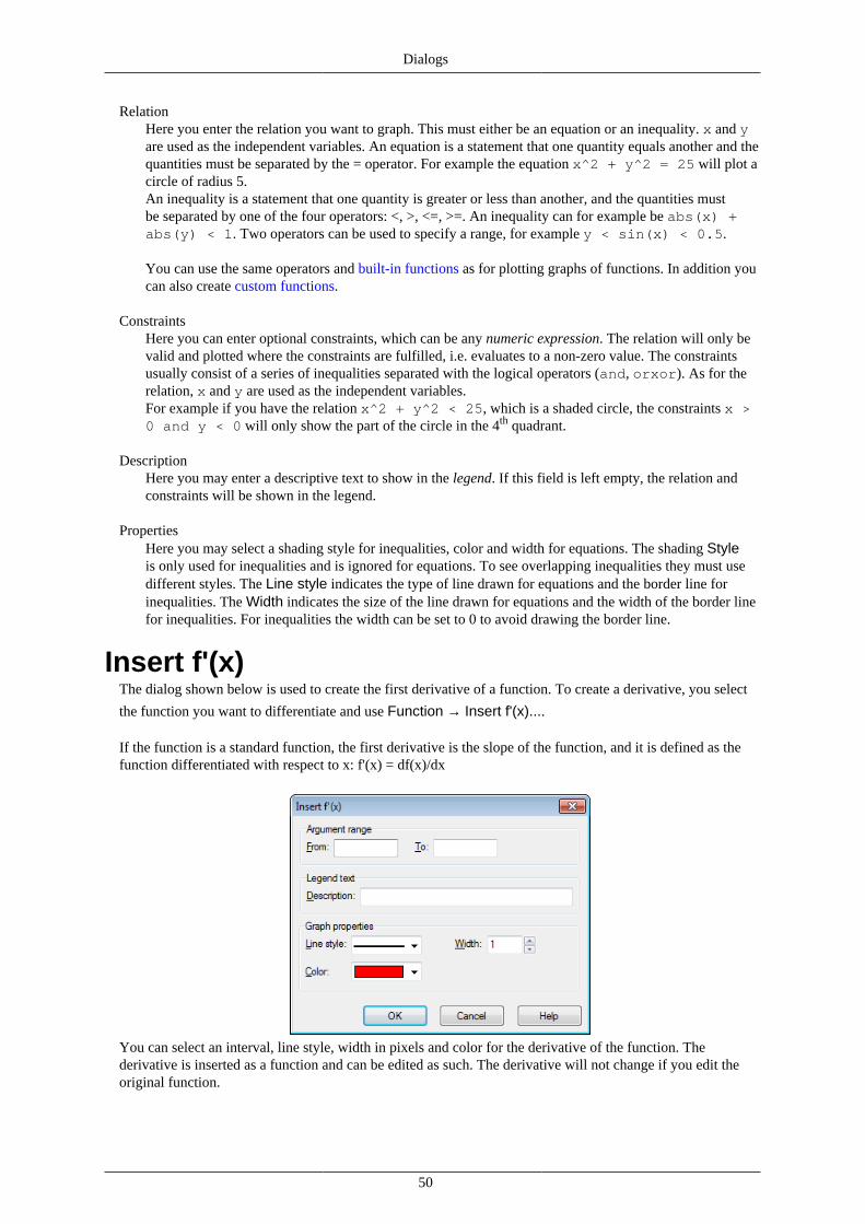
Dialogs

50

RelationHere you enter the relation you want to graph. This must either be an equation or an inequality. x and yare used as the independent variables. An equation is a statement that one quantity equals another and thequantities must be separated by the = operator. For example the equation x^2 + y^2 = 25 will plot acircle of radius 5.An inequality is a statement that one quantity is greater or less than another, and the quantities mustbe separated by one of the four operators: <, >, <=, >=. An inequality can for example be abs(x) +abs(y) < 1. Two operators can be used to specify a range, for example y < sin(x) < 0.5.

You can use the same operators and built-in functions as for plotting graphs of functions. In addition youcan also create custom functions.

ConstraintsHere you can enter optional constraints, which can be any numeric expression. The relation will only bevalid and plotted where the constraints are fulfilled, i.e. evaluates to a non-zero value. The constraintsusually consist of a series of inequalities separated with the logical operators (and, orxor). As for therelation, x and y are used as the independent variables.For example if you have the relation x^2 + y^2 < 25, which is a shaded circle, the constraints x >0 and y < 0 will only show the part of the circle in the 4th quadrant.

DescriptionHere you may enter a descriptive text to show in the legend. If this field is left empty, the relation andconstraints will be shown in the legend.

PropertiesHere you may select a shading style for inequalities, color and width for equations. The shading Styleis only used for inequalities and is ignored for equations. To see overlapping inequalities they must usedifferent styles. The Line style indicates the type of line drawn for equations and the border line forinequalities. The Width indicates the size of the line drawn for equations and the width of the border linefor inequalities. For inequalities the width can be set to 0 to avoid drawing the border line.

Insert f'(x)The dialog shown below is used to create the first derivative of a function. To create a derivative, you select

the function you want to differentiate and use Function → Insert f'(x)....

If the function is a standard function, the first derivative is the slope of the function, and it is defined as thefunction differentiated with respect to x: f'(x) = df(x)/dx

You can select an interval, line style, width in pixels and color for the derivative of the function. Thederivative is inserted as a function and can be edited as such. The derivative will not change if you edit theoriginal function.

Dialogs

51

Custom functions/constantsGraph allows you to define your own custom functions and constants, which you can use in other expressionsin the program. You may want to use this to factor out frequently used constants and subexpressions to make

it faster and easier to use these items. Use the Function → Custom functions... menu item to show thedialog.

Entering functionsThe function and constant names are entered in the first column. The name may contain any combinationof letters, digits and underscore but it must always start with a letter. You may not use a name that isalready assigned to a built-in function or variable.Function arguments are entered after the name in brackets separated by comma, e.g. f(x,y,z) is afunction named f taking three arguments named x, y and z. Like the function name, the argument namesmust start with a letter and only contain letters and digits.

The expressions you want to define are entered in the second column. The expressions can use thearguments specified in the first column and all built-in functions, other custom functions and constants,and even call themselves recursively. A comment can be written after a # symbol at the end of anexpression.

Changing and removing functionsYou can remove a function or constant by clearing the name and definition or selecting Remove rowfrom the context menu. All elements using the deleted function or constant will fail when evaluated.

When you press OK or Apply in the shown dialog, all elements are updated to reflect any changes to thefunctions and constants.

EvaluateThis dialog is used for interactive calculations on functions. The dialog may be docked below the functionlist, which is default, or undocked as a floating dialog.

EvaluateWhen Calc → Evaluate is selected the dialog is used to evaluate the selected function at a given value eitherentered in the dialog or traced with the mouse.

Below you can see the dialog, that appears when a standard function is selected. The dialog will look a littledifferent when a parametric function, polar function or tangent is selected.

Dialogs

52

You can enter a value for which you want to evaluate the function. The value will be evaluated for thefunction selected in the function list. If the result is on the graph within the shown coordinate system, it willbe marked with a dashed cross. You can also trace the drawn graph with the mouse. Just click on the graphwith the mouse and the function will be evaluated at the nearest point.

It may happen that the result of an evaluation is a complex number with an imaginary part. This number will

either be written as a+bi, a∠θ or not written at all depending of the choice under Options.

When you click with the mouse on the graphing area you may choose what the cursor will snap to:

FunctionThe cursor will snap to the nearest point of the selected function.

IntersectionThe cursor will snap to the nearest intersection between the selected function and every functiondisplayed (including the function itself).

x-axisThe cursor will snap to the nearest intersection between the selected function and the x-axis.

y-axisThe cursor will snap to the nearest intersection between the selected function and the y-axis. Notavailable for standard functions.

Extreme x-valueThe cursor will snap to the nearest local extreme value for the x-coordinate. Not available for standardfunctions.

Extreme y-valueThe cursor will snap to the nearest local extreme value for the y-coordinate.

AreaWhen Calc → Area is selected the dialog is used to calculate the area for the selected function over aspecified domain range. For standard and parametric functions and tangents the area is the signed areabetween the graph and the x-axis (the real x-axis and not necessarily the visible one) for the given range.The area below the x-axis is considered negative. For standard functions and tangents, this is the same as thedefinite integral.

For polar functions, the area is the one between the graph in the given range and the origin. The area isconsidered negative when the angle goes from a higher to a lower value (clockwise).

You can either enter the range in the edit boxes or select the range with the mouse. The calculated area willbe shown below the range, and the matched area will be marked with a shading in the coordinate system. Thecalculation is done using the Gauss-Kronrod 21-point integration rule adaptively with as much accuracy aspossible. If an estimated relative error less than 10-4 cannot be reached, no result will be shown.

Length of pathWhen Calc → Length of path is selected the dialog is used to calculate the distance between two points onthe function along the curve. You may either enter the range in the dialog or use the mouse to mark it. The

Dialogs

53

range will be marked in the coordinate system. The calculation is done by converting it to an integration andusing Simpson's formula through 1000 iterations.

TableThe dialog shown below is used to evaluate the selected function for a range. First select a function in the

function list and use the menu item Calc → Table to show the dialog. You specify the first and last value

of the independent variable in the From and To fields. In the ∆x or ∆t field you specify the increment of theindependent variable at each evaluation.

When you press the Calc button, the table will be filled with the independent variable in the first column. Therest of the columns depend on the type of function. For a standard function, the table will show f(x), f'(x) andf''(x). For a parametric function, the table will show x(t), y(t), dx/dt, dy/dt and dy/dx. For a polar function, thetable will show r(t), x(t), y(t), dr/dt and dy/dx. Unneeded columns can be hidden from the context menu. If thecalculations takes a long time, a progress indicator will be shown.

You can select some cells with the mouse and right click with the mouse and use Copy from the contextmenu to copy the cells to the clipboard. From the clipboard the data may be pasted into another program, e.g.Microsoft Excel.

When you move the mouse to the left side of the table the mouse pointer changes to a right pointing arrow.Now you can select whole rows with the mouse. When you move the mouse to the top of the table, thepointer changes to a down pointing arrow. Now you can select whole columns with the mouse. The wholetable may be selected by right clicking and selecting Select all. It is also possible to select cells by holdingdown the Shift key and using the arrow keys on the keyboard.

From the context menu it is also possible to export the selected data to a file as comma or tab delimited text.

Note that if you choose to create a lot of values in the table, it may take some time to calculate them. Manyvalues may also take up a lot of memory from the system.

Dialogs

54

AnimateThis dialog is used to create an animation by changing a custom constant. The animation can be playeddirectly, saved to a file or copied into a document. The animation can contain all elements supported byGraph, for example functions, relations, point series, labels, etc.

ConstantHere you select which constant you want to change in the animation. The constant must already havebeen created in the Custom functions/constants dialog. The selected constant will be changed in eachframe in the animation.

RangeIn the From and To fields you need to specify the range of the selected constant in the animation. TheStep value indicates how much the constant is changed between two frames. The number of frames isgiven by (To - From) / Step. More frames will give a smoother animation but it will also take longer tocreate and take up more space in the disk file.

Frame informationYou can specify the image size of the animation. This will affect the file size and the time it takes tocreate the animation. The Frames/second indicates the default speed of the animation. Most playerswill be able to adjust the speed when the animation is played.

When you press the Animate button, an animation is created from the settings you have specified. This maytake some time depending on what elements exist in the coordinate system and how many frames are needed.

When the animation is finished, a very simple player is shown. You can use this to play the animation. The button will give you some additional options.

SpeedHere you can change the playback speed. This will only affect the playback and not the file saved.

RepeatWhen checked the animation will continue playing. When finished it will start over again.

Auto reverseThis will make the animation run backwards when it reaches the end. This is most useful in combinationwith the Repeat option, which will make the animation oscillate between the two ends.

Save as...This will save the animation as an Audio Video Interleave (avi) file, which can be played by any mediaplayer.

Dialogs

55

Save frame...This will save the currently shown frame as a bitmap file. This can be either Windows Bitmap (bmp),Portable Network Graphics (png) or Joint Photographic Experts Group (jpeg).

Save all frames...This will save all frames as single bitmap files. This is the same as repeating Save frame... for eachframe in the animation.

Save as imageUse the menu item File → Save as image... to save the shown coordinate system as an image file. Whenthe menu item has been chosen, a standard Save As dialog will appear. In this dialog you write a filename,choose a directory and select one of the following image types:

Windows Enhanced Metafile (emf)Metafiles are usually preferred because they are small and look nice even when scaled. Though emf filesare widely supported under MS Windows, they are not very portable.

Scalable Vector Graphics (svg)This is a format for portable metafiles and should therefore be preferred for files placed on the Internet.However the format is still not supported by all browsers.

Portable Network Graphics (png)Portable Network Graphics (png) is a format that is better compressed than bmp files. This is the mostsustainable format for web pages, because it is small and can be understood by all browsers.

Windows Bitmap (bmp)Windows Bitmap (bmp) is a standard format supported by almost all Windows programs that can readgraphics files.

Joint Photographic Experts Group (jpeg)Joint Photographic Experts Group (jpeg) is a bitmap format with loss. It is supported but notrecommended because graphs will usually become blurred.

Portable Document Format (pdf)Portable Document Format (pdf) is actually not an image format. It is a way to store documents aspostscript in a portable way. Graph will store the image as Portable Network Graphics inside the pdf file.

The Options... button in the save dialog can be used to change the image size. You may also be able tochange other settings depending on the chosen image format.

Import point seriesGraph can import point series from text files where the values are delimited by comma, semicolon, space or

tabulator. You use File → Import → Point series... and select the file to import. If you do not specify thetype of file, Graph will try to guess the delimitor.

The simplest file looks like this, which uses comma as delimitor:

1,1.72,4.33,9.54,16.2

When imported you get a point series with the coordinates: (1,1.7), (2,4.3), (3,9.5), (4,16.2)

A file with more than two columns will be imported as several point series with the same x-coordinates asspecified in the first column. Here is an example with semicolon as delimitor:

50;71,8113997;78,23883162;79,17509098;78,58979676;78,62449077;78,2374541;77,763769655;71,81941659;78,17869416;79,2155277;78,48195769;78,6005272;78,22113423;77,7874084

Dialogs

56

60;71,82943769;78,12714777;79,24787707;78,55661551;78,51266076;78,2129743;77,842565665;71,82866684;78,08419244;79,20744036;78,54002489;78,56857576;78,22929417;77,818926870;71,81448312;78,06701031;79,18317833;78,55661551;78,55260005;78,24561404;77,75589

When imported you get 7 point series which all share the same x-coordinates.

You can name the point series by starting the line before the data with # followed by the names separatedby the same separator as the data. This can also be used for creating several point series that do not sharethe same x-coordinates by separating the point series with a # and optionally a name for the following pointseries. The following shows an example with space as separator:

#a b0 0.2 0.51 1.4 -1.72 2.1 -2.63 3.8 -3.3#d e4 4.3 -4.15 5.8 -5.56 6.1 -6.17 7.9 -7.6

This will create four point series each with four data points named a, b, c and d. a and b will share the same x-coordinates, and c and d will share the same x-coordinates.

Not only numbers, but any valid expression can be imported. The following shows an example withsemicolon:

1;sin(0.1)2;sin(0.2)3;1+sin(0.3)pi;2*sin(pi/2)

57

PluginsTo use the plugin system in Graph you need to install Python 3.2 from http://www.python.org.Documentation of the Python language may be found installed with Python or online [http://docs.python.org/3.2/].

PluginsPlugins are Python scripts and are usually distributed in source form as .py files but the can also be distributedas compiled .pyc files. The plugin files are placed in the Plugins directory where Graph is installed, andwill automatically be found and loaded by Graph.

WarningPlugins are scripts, which are just small programs that run inside Graph and interacts withGraph. But a plugin can do anything that a program with the same rights can do. This meansthat if Graph is run with administrator rights, it is possible to write a plugin that erases the wholehard disk. Therefore you should be careful about which plugins you use and only install pluginsfrom a trusted source, or at least you should check the source code for suspicious parts.

Python interpreterThe plugin system also gives access to a Python interpreter by pressing F11. In this interpreter you can writePython expressions and that way do very advanced things in Graph. It is also an easy way to test code beforeit is used in a plugin.

58

AcknowledgementsLibraries

dxgettextTranslation library.Copyright © Lars B. Dybdahl et al.http://dybdahl.dk/dxgettext/

PDFlib-LiteUsed to create PDF files.Copyright © 1997-2005 Thomas Merz & PDFlib GmbHhttp://www.pdflib.com

PythonUsed for plugin support and advanced interaction.Copyright © 2001-2006 Python Software Foundationhttp://www.python.org

GNU Scientific LibraryNumerical library.Copyright © 2009 Free Software Foundation, Inc.http://www.gnu.org/software/gsl/

BoostPeer-reviewed C++ library.http://www.boost.org

Acknowledgements

59

Translations

Language Program Help file Translators

Arabic Yes No Abdellah Chelli

Basque Yes No Xabier Maiza

Chinese(Simplified)

Yes No Lala Sha

Chinese(Traditional)

Yes No Jian-Jie Dong

Croatian Yes Yes Hasan Osmanagić

Czech Yes No Pavel SimerkaMartin StružskýPavlína Krausová

Danish Yes Yes Michael Bach IpsenErik Lyngholt Nielsen

Dutch Yes Yes Etienne Goemaere

English Yes Yes Ivan Johansen

Finnish Yes No Pekka Lerssi

French Yes Yes Jean-Pierre Fontaine

German Yes Yes Frank HüttemeisterSebastian StützMichael Bach Ipsen

Greek Yes Yes Dimitris Spingos (Δημήτρης Σπίγγος)Theodoros Kannas

Hungarian Yes No Gabor Magyari

Italian Yes Yes Alessandro SerenaAttilio Ridomi

Korean Yes No Choe Hyeon-gyu

Mongolian Yes No Batnasan Davaa

Norwegian Yes No Tore Ottinsen

Persian Yes No Shayan AbyariYashar PourMohammad

Polish Yes No Paweł Baczyński

Portuguese(Brazil)

Yes Yes Jorge CostaMaraFernandaDeivid e MonalisaWladimir A. SilvaAldemar C. Filho

Portuguese(Portugal)

Yes No Jorge Geraldes

Russian Yes No Ilya A.Ivans Leonovs

Serbian Yes No Jasmina MalinovicBranimir Krstic

Slovenian Yes Yes Jernej BašaRok Štokelj

Acknowledgements

60

Language Program Help file Translators

Barbara PušnarSergej Pušnar

Spanish Yes Yes Francisco OliverAlejandro Arce

Swedish Yes No Pär SmårsMichael Bach Ipsen

Turkish Yes No Mumtaz Murat Arik

Vietnamese Yes No Trung

DonatorsSebastian Albrecht, specializing in the Vancouver Special [http://yourvancouverrealestate.ca/vancouver-special/]Sothebys real estate Toronto [http://partnershiptoronto.com/]Chantal Marr, a Canadian life insurance [http://lsminsurance.ca/canadian-life-insurance-companies] expertElli Davis, a Toronto MLS Listings [http://ellidavis.com/mls-listings] expert

MiscellaneousThe icon for Graph was designed by Jonathan Holvey.

61

Glossarycomplex number

Complex numbers are a superset of real numbers. Complex numbers are two dimensional and is mostoften written on rectangular form as a+bi where a is the real part and b is the imaginary part. The

imaginary unit i is defined as i^2=-1. Complex numbers can also be shown on polar form as a∠θ where a

is the absolute value of the number and θ is the angle of the number in radians or degrees.Complex numbers are used in the Evaluate dialog for standard functions and for graphing functionswhen Calculate with complex numbers is enabled under the Settings tab in the Edit axes dialog.

function listThe function list is shown in the left side of the main window. This list shows a list of all functions,tangents, point series, shadings and relations. When you want to manipulate an item, you first have toselect it. The selected item is normally marked in blue, but it will be marked in gray when somethingother than the function list has focus. You can manipulate the selected element through the Functionmenu or through the context menu appearing when you right click on the element.

graph elementA graph element is something that is shown in the coordinate system. This can be a function, point series,label, relation, etc. The graph elements are also shown in the function list where they can be manipulatedfrom the Function menu or the context menu.

integerThe set of numbers ...,-3,-2,-1,0,1,2,3,... is called integers and is a subset of the real numbers. A giveninteger n may be negative, zero or positive.

legendThe legend is a box that per default is placed at the upper right corner of the graphing area, and shows alist of the plotted functions, tangents, shadings, and point series in the coordinate system. Select Showlegend under Settings in the Edit axes dialog to show the legend. Right click on an item in the functionlist and deselect Show in legend if you don't want the item shown in the legend. When editing an itemyou can enter the text to be shown in the legend. For functions and tangents the function equation will beshown if no legend text is entered.

numeric expressionAn expression that can be evaluated as a number is called a numeric expression. The expression caninclude any combination of numbers, constants, variables, operators and functions.

radiansRadians are a way to describe the size of an angle similar to degrees, but radians are not a unit like

degrees. The angle of a whole circle is 360° or 2π radians. An angle in radians can be converted to

degrees by multiplying with 180°/π. An angle in degrees can be converted to radians by multiplying with

π/180°. You can choose to use radians or degrees for trigonometric functions in the Edit axes dialogunder the Settings tab.

real numberA real number is on the form nnn.fffEeee where nnn is the whole number part that may be negative. fffis the fraction part that is separated from the integer part with a dot '.'. The fraction part is optional, buteither the integer part or the fraction part must be there. E is the exponent separator and must be an 'E' inupper case. eee is the exponent optionally preceded by '-'. The exponent is only needed if the E is there.Notice that 5E8 is the same as 5*10^8.