Verification

Reference books

Reference books

An Invitation to Design Verification• Verification engineer should understand specification as well as

design.

• Verification engineer should follow the different design approach.

• Statistical data show that around 70% of the project development cycle is devoted to design verification

• In general, design verification encompasses many areas, such as functional verification, timing verification, layout verification, and electrical verification etc.

Design, Validation and Testing

Some basic terms

Set of Specifications

Implementation

Design Process Transforms

Specification--The specification state the functionality that the design executes but does not indicate How it executes.

Design—The meaning of verb design

Implementation: Spells out the details of how the functionality

is provided. Both specification and implementation are a

form of description of functionality but they have different level of abstraction.

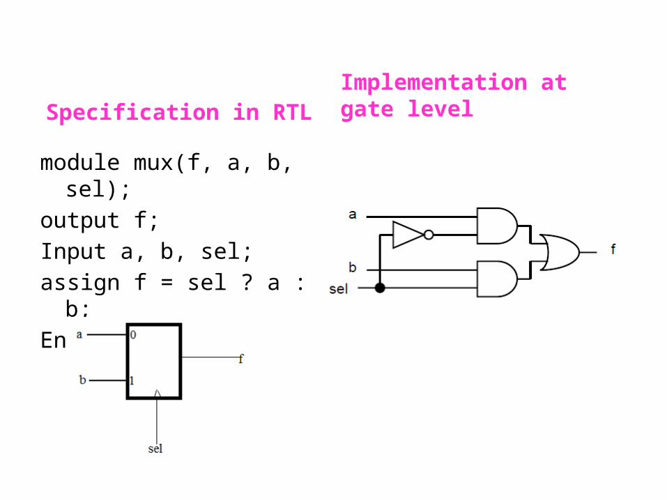
Specification in RTL

module mux(f, a, b, sel);output f;Input a, b, sel;assign f = sel ? a : b;Endmodule;

Implementation at gate level

Design Validation: Means establishing that the system does what it was intended to

do. It essentially provides a confidence in the system’s operation.Or

Verification is different than validation; the objective of validation is to prove that it indeed works as intended.

Design validation of SoC can be considered as validation of hardware operation, validation of software operation and validation of combined system operation.

This includes both functionality and timing performance at the system level.

Design and Verification

Whether the design is specifying the design intent.

What Is Design Verification?• Verifications means checking against an accepted entity-

generally, a higher level of specifications.

Or Whether the specification is correct? Whatever in specification is implemented properly? Whatever prototype we developed is correctly

implementing the design intent?

• In IC design, verification is divided into two major tasks

(1) Specification verification-Specification verification is done to verify that during system design, the translation from one abstraction level to the other is correct and the two models match each other.

(2) Implementation verification--The objective of implementation verification is to find out, whether the system will work after implementation.

Design challenge in verification

• Suppose we want to design a pacemaker

Minimize the delay

Minimize area

Minimize power (upf, cpf)

Improve verifiability

Improve reliability

Improve testability

Reduce cost

Optimization during synthesis

Verification reliability and coverage

Algorithms for better yieldTest automation and DFT

Resource optimization

• CPF=common power format• UPF=unified power format

Abstraction level of Digital design

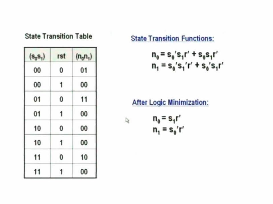
Design example: 2 bit gray counter

Gray Counter: Successive values should differ only in one bit. Reset signal resets the counter to zero.

State machine representation

A ladder of design abstraction

Abstraction spectrum of the design

• Specification has a higher level of abstraction means less details than implementation.

• In an abstraction spectrum of design, decreasing order of abstraction: functional specification, algorithmic description, register-transfer level (RTL), gate netlist, transistor netlist, and layout .

• The process of turning a more abstract description into a more concrete description is called refinement.

• Therefore, a design process refines a set of specifications and produces various levels of concrete implementations.

The relationship between design and verification

• Design verification is the reverse process of design. It starts with an implementation and confirms that the implementation meets its specifications.

• For every step of design, there is a corresponding verification step. For example, a design step that turns a functional specification into an algorithmic implementation requires a verification step to ensure that the algorithm performs the functionality in the specification.

Design verification can be classified into two types.

• Equivalence checking - verifies that two versions of design are functionally equivalent.

• Model checking, Implementation verification, property checking—means checking the model against properties

Are the Two Circuits Equivalent?

1. Map key points: inputs, outputs, f1 ↔f3, f2 ↔f42. Build equations: f3 = b, f2 = f1, out = (a · f2)

f3 = b, f4 = (f3), out = a + f43. Compare equations: show logic of output signals is the same

Equivalence Checking

In this case, the comparison of the equations will show that (f1 = b = f3) for the both circuits, and (f2 = f1 = f3) for the top, while (f4 = f3) for the bottom circuit which means, f2 ≠ f4 → ERROR

Property checkingwhat is formal property and formal verification?Toy example: Priority encoder

Here r1, r2 request lines and g1, g2 are grant lines. Some properties of the arbiter in Linear Temporal Logic are given as1. Either g1 or g2 is always false (mutual exclusion)

2. Whenever r1 is asserted, g1 is given in the next cycle.

3. When r2 is the sole request, g2 comes in the next cycle.

4. When none are requesting , the arbiter parks the grant on g2.

RTL designer has given this implementation

Two implementation those are not equivalent

• Specification is incomplete

Design an arbiter with the following property

1. Whenever r1 is raised, the arbiter must assert g1 within the next two cycles.

2. Whenever r2 is raised, the arbiter must eventually assert g2.

3. The grant lines g1 and g2 are never asserted together.

Neither reads r1 nor r2 !!

Reads r1 but not r2 !!

• There are two types of design error(i) The first type of error introduced during an

implementation process. (ii) The second type of error exists in the specifications.

To prevent this type of error, we can use a software program to synthesize an implementation directly from the specifications.

Eliminates most human errors, errors can still result from bugs in the software program, or usage errors of the software program may be encountered.

The Basic principle of verification design

Redundancy -- Another method the more widely used method to reveal errors

• That is, the same specifications are implemented two or more times using different approaches, and the results of the approaches are compared.

• In theory possible but in practice, more than two approaches is rarely used, because more errors can be introduced in each alternative verification, and costs and time can be insurmountable.

The basic principle of design verification. (A) The basic methodology of verification by redundancy.

The Basic Verification Principle• The design process can be regarded as a path that

transforms a set of specifications into an implementation.

• The basic principle behind verification consists of two steps.

(i) Verification transformation- there is a transformation from specifications to an implementation.

(ii) During the second step, the result from the verification is compared with the result from the design to detect any errors.

The basic principle of design verification. (A) The basic methodology of verification by redundancy. (B) A variant of the basic methodology adapted in model checking. (C) Simulation methodology cast in the form of verification by redundancy.

Property Checking based verification

The basic principle of design verification. (B) A variant of the basic methodology adapted in model checking. See previous slide of property checking

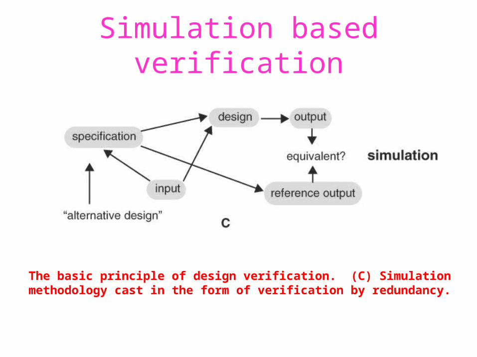
Simulation based verification

The basic principle of design verification. (C) Simulation methodology cast in the form of verification by redundancy.

• It consists of four components: the circuit, test patterns, reference output, and a comparison mechanism.

• The circuit is simulated on the test patterns and the result is compared with the reference output.

• The implementation result from the design path is the circuit, and the implementation results from the verification path are the test patterns and the reference output.

• The reason for considering the test patterns and the reference output as implementation results from the verification path is that, during the process of determining the reference output from the test patterns, the verification engineer transforms the test patterns based on the specifications into the reference output, and this process is an implementation process.

• Finally, the comparison mechanism samples the simulation results and determines their equality with the reference output.

Verification Methodology1. Simulation based verification (Existence of input vectors,

Simulation is input oriented (the designer supplies input tests))

2. Formal method based verification (Absence of input vectors, Formal method are output oriented(the designer supplies the output properties to be verified)

3. A hybrid called semiformal verification (combination of simulation-based and formal technology, takes in input vectors and verifies formally around the neighborhood of the vectors).

Functional verification challenge

Q. Is the implementation correct?

How do we define the correct?

Classical: Simulation results matches with golden output. Required CKT, i/p pattern, reference output, comparison mechanism.

Formal: equivalence with respect to a golden model

Property verification: Correctness properties (assertions) expressed in a formal language

Formal: model checking Semi formal: Assertion based verification

Tradeoff between computation complexity and exhaustiveness.

Simulation based verification

Test plan— that details the specific functionality to verify so that the specifications are satisfied.

Or what need to be tested ? Mostly written in english

language document.• It consists of features, operations, corner cases

etc. Linter: checks the static and potential errors in your

code and coding style violations. It does not require input vectors.

Test bench: a wrapper around the design which invoke several tests.

• Regression is an abnormal state in which development has stopped prematurely.

• In a bug tracking system, the bug goes through several stages: from opened to verified, fixed, and closed.

• A bug tracking system allows the project manager to prioritize bugs and estimate project progress better.

Formal Method-Based Verification

Formal Properties

always @ (posedge clk)begin if (!rst) begin

a1<=a2;a2<=a3;end; end

Gate level

Transistor level

Design intent

RTLModel checking

Logical Equivalence checking

Goal: Exhaustive verification of the design intent within feasible time limits

Philosophy: Extraction of formal models of the design intent and the implementation and comparing them using mathematical/logical methods.

• Formal properties are presented by Temporal logic.

• Magellan for Synopsys and (Incisive formal verifier) IFV for Cadence.

Formal Method-Based Verification

A typical flow of formal verification

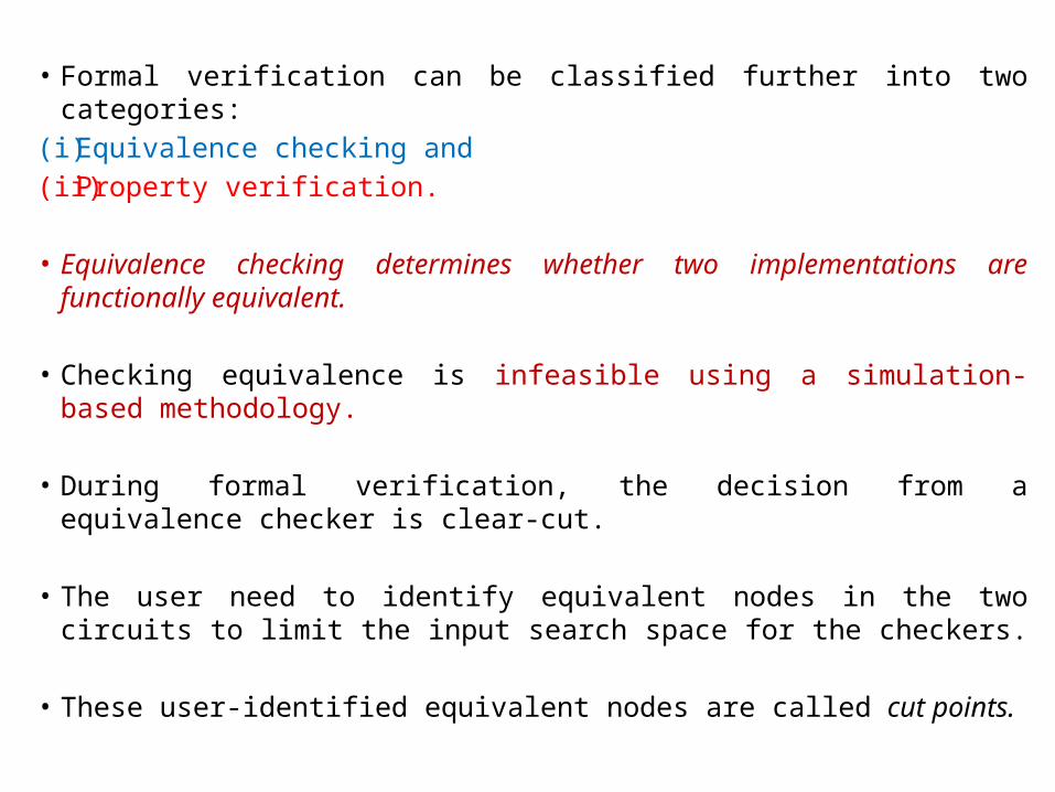
• Formal verification can be classified further into two categories:(i) Equivalence checking and (ii) Property verification.

• Equivalence checking determines whether two implementations are functionally equivalent.

• Checking equivalence is infeasible using a simulation-based methodology.

• During formal verification, the decision from a equivalence checker is clear-cut.

• The user need to identify equivalent nodes in the two circuits to limit the input search space for the checkers.

• These user-identified equivalent nodes are called cut points.

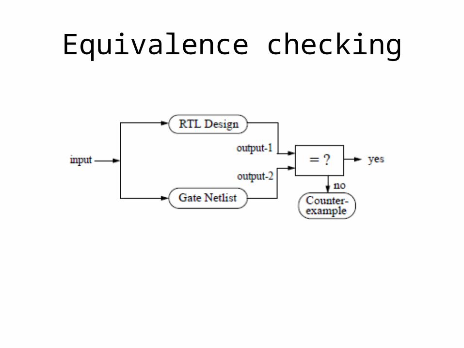
Equivalence checking

Two approaches of equivalence checking

• SAT (satisfiability)--searches the input space in a systematic way for an input vector or vectors that would distinguish the two circuits (akin to ATPG).

• ROBDD--Converts the two circuits into canonical representations, and compare them.

• A canonical representations are isomorphic in nature.

• Binary decision diagrams of two equivalent functions are graphically isomorphic.

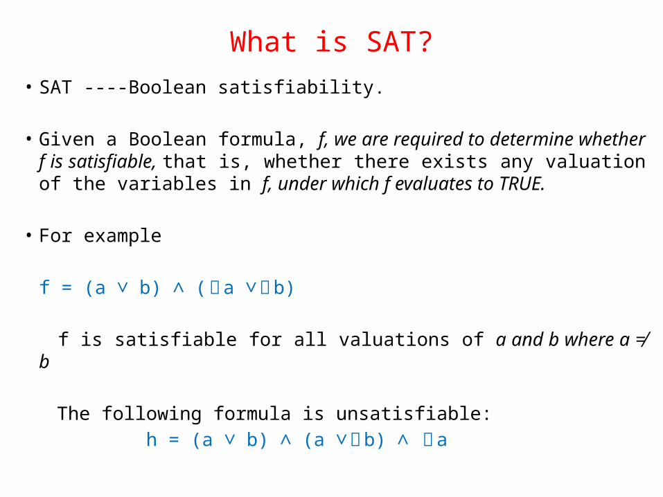
What is SAT?• SAT ----Boolean satisfiability.

• Given a Boolean formula, f, we are required to determine whether f is satisfiable, that is, whether there exists any valuation of the variables in f, under which f evaluates to TRUE.

• For example

f = (a b) (∨ ∧ ￢ a ∨￢ b)

f is satisfiable for all valuations of a and b where a ≠ b

The following formula is unsatisfiable: h = (a b) (a ∨ ∧ ∨￢ b) ∧ ￢ a

Equivalence Checking Problem• Two designs are to be functionally equivalent if they

produce identical output sequence for all input sequences

• Whether two combinational logic designs are equivalent?

• How to do the equivalence checking in sequential circuit?

A

A

NOR

a

bf NOTa g

• Sequential equivalence checking Compare state machines

• Combinational equivalence checking Compare combinational Boolean functions

If a one to one corresponds is given between the register then sequential checking can be solved using combinational equivalence checking.

Two designs are to be functionally equivalent if they produce identical output sequence for all input sequences.

Two designs are to be functionally equivalent if they produce identical output sequence for all input sequences.

Property Checking• Property checking takes in a design and a property

which is a partial specification of the design, and proves or disproves that the design has the property.

• A property is essentially a duplicate description of the design, and it acts to confirm the design through redundancy.

• A program that checks the property is called a model checker

Property Checking

The FPV Approach

RTL Formal Property Verification

• The idea behind property checking is to search the entire state space for points that fail the property.

• If a such point is found, the property fails and the point is a counterexample.

• Next, a waveform derived from the counterexample is generated, and the user debugs the failure. Otherwise, the property is satisfied.

• Symbolic traversal algorithms that enumerate the state space implicitly.

• That is, it visits not one, but a group of points at a time, and thus is highly efficient.

Property checking (informally)

P1: G[ r1 Xg1 XXg1 ]⇒ ∧P2: G[ ￢ g1 g2 ]⇒P3: G[ ￢ g1 ∨ ￢ g2 ]P4: G[ ￢ r1 X∧ ￢ r1 XX⇒ ￢ g1 ]

It is easy to see (informally) that the implementation has at least two bugs:

• It refutes P1 when r1 is high for only one cycle. The arbiter asserts g1 for only one cycle, where as P1 requires g1 to be high for two consecutive cycles.

• If r1 and r2 are both low at some time, then P2 fails in the next cycle since both g1 and g2 are low.

Determine state machine equivalence between the machines in A and B.

Simulation-Based Verification versus Formal Verification

• Simulation-based verification requires input vectors and formal verification does not.

• The mind-set in simulation-based verification is first to generate input vectors and then to derive reference outputs.

• In formal verification process the user starts out by stating what output behavior is desirable and then lets the formal checker prove or disprove it. Users do not concern themselves with input stimuli at all.

• Simulation-based methodology is input driven and the formal methodology is output driven.

Model Checking vs. Simulation

• Formal verification is exhaustive, in the sense that it does not miss any point in the input space a problem from which simulation-based verification suffers.

• However, this strength of formal verification sometimes leads to the misconception that once a design is verified formally, the design is 100% free of bugs.

An output space perspective of simulation-based verification versus formal verification

verification through input space sampling. Unless all points are sampled, there exists a possibility that an error escapes verification. While, formal verification works at the property level. Given a property, formal verification exhaustively searches all possible input and state conditions for failures.

• If viewed from the perspective of output, simulation-based verification checks one output point at a time;

• formal verification checks a group of output points at a time (a group of output points make up a property).

• Therefore, to verify completely that a design meets its specifications using formal methods, it must be further proved that the set of properties formally verified collectively constitutes the specifications.

• The fact that formal verification checks a group of points at a time makes formal verification software less intuitive and thus harder to use.

• A major disadvantage of formal verification software is its extensive use of memory and (sometimes) long runtime before a verification decision is reached.

• When memory capacity is exceeded, tools suffers problem.

• As a result, formal verification software is mostly applicable only to circuits of moderate size, such as blocks or modules.

Property Verification

• First define formal specification

• The two broad methodologies for property verification, namely are

(i) Dynamic Assertion Based Verification (ABV) and (ii) Formal Property Verification (FPV).

An arbiter implementation

Implementation Verilog code

The Dynamic ABV Approach

• To drive input of the implementation we required test bench.

• Complexity increases due to other modules and protocols for communication.

• It is not practically feasible to write directed tests to sensitize all possible behaviors of this model.

Dynamic ABV

Assertion-based Verification Platform

• Simulate the implementation with the test bench. • The assertion checker reads the signals in the

interface and monitors the status of the properties.• If any of the properties fail during the simulation, the

checker reports it immediately. • The failure points help the verification engineer to

isolate the source of the bug.There are two key features of dynamic ABV- (i) It is built over the traditional simulation framework

and requires nominal additional effort from the verification engineer.

(ii) Secondly, Capacity Concerns since the verification is done over the simulation run.

• The main criticism of the dynamic ABV approach is that only those behaviors that are covered by simulation are examined for property violation.

• Objective: suppose the implementation for a given arbiter is given as below. The problem is to determine whether this implementation satisfies formal specification.

Simple Test-Bench fragment for arbiter

A simplified test environment for arbiter consists of a clock generator, and models for the two requesting devices.

• Consider the case when both requests are low for two consecutive cycles and the specification demands that the grant be parked on g2 (by default),

• Verify: but in implementation both grants will be low.

• Result: Hence the implementation of arbiter has a bug.

• So, the bug will escape detection because the test bench never creates the relevant cases.

• This example brings out one of the major challenges in property verification.

• In order to achieve a meaningful level of functional coverage, the industry is moving towards coverage driven randomized test generation.

• This helps in reaching a high level of coverage in short time, but the difficult corner case behaviors are typically left out.

• Formal properties target these corner case behaviors, but dynamic ABV is not effective unless we can force the test bench to create the relevant scenarios.

The FPV Approach

RTL Formal Property Verification

The FPV Approach• The heart of this approach is a model checking tool.

• A model checking algorithm has two main inputs – (i) a formal property and a (ii) finite state machine representing the implementation.

• The role of the algorithm is to search all possible paths of the state machine for a path which refutes one or more properties.

• If one exists, then the path trace is reported as the counter-example.

• Otherwise the model checker asserts that the property holds on the implementation.

Example. Let us again consider the implementation of arbiter and its state machine are shown below. The transitions are labeled by the inputs that enable the transition. The symbol ”x” indicates that the value of the signal is a don’t care.

• The model checker will find a refuting path for the below given property

• Since the path also contains the input sequence for which the refutation occurs, it produces a complete counter-example trace with the appropriate inputs that trigger the incorrect behavior of the module.

Formal Property Verification Platform

Problem: The main limitation of model checking technology is in capacity.

• Typically the main bottleneck is in the size of the FSM extracted from the implementation.

• The number of states in the machine typically grows exponentially with the number of concurrent components.

Solution:1. BDD based approach2. Bounded model checking

Languages for Temporal Properties

• PSL (Property Specification Language)/SVA. (System-Verilog Assertions)

• The formal introduction to a language has two main parts, namely the syntax and the semantics.

• The syntax defines the grammar of the language – it tells us how we may construct properties using the basic set of signals and operators.

• The semantics define the meaning of the properties.

Propositional logic

• Propositions are statements that may be basically true or false.

• Example. if it is raining and Ram does not have his umbrella then he will get wet. Ram is not wet. It is raining.

• Therefore Ram has his umbrella.• If p and not q then r. Not r, p therefore q.

Temporal logic

Formal verification makes sense only when we have a formal specification

• the functionality of all digital circuits may be formally expressed in terms of Boolean functions.

• For example, a half adder

Half Adder

a

b

s

c

• Given: An implementation of a half adder in Verilog RTL and the above equations,

• Problem: Apply formal verification whether the RTL is correct.

• Solution: Translating both the RTL and the Boolean functions into some canonical representation of Boolean functions and then by checking whether the representations are isomorphic.

• There is a wide range of choices for Boolean function representation, including Binary Decision Diagrams (BDD), Binary Momemt Diagrams (BMD) etc.

Two implementation those are not equivalent

• Specification

Design an arbiter with the following property

1. Whenever r1 is raised, the arbiter must assert g1 within the next two cycles.

2. Whenever r2 is raised, the arbiter must eventually assert g2.

3. The grant lines g1 and g2 are never asserted together.

The arbiter simply asserts g1 and g2 in alternate cycles – regardless of the status of the request lines. Neither reads r1 nor r2 !!

Whenever r1 is raised, the arbiter asserts g1 in the next cycle. In all other cycles, it asserts g2. Reads r1 but not r2 !!

Now compare the nature of this specification with the half adder.

In both cases it is possible to have more than one implementation, which satisfies the specification. Let us consider the following two implementations of the arbiter as in previous slide.

Result: It is obvious that these two implementations are not logically equivalent, that is, the Boolean functions representing their functionality are not identical.

On the other hand, by specifying the Boolean functions for the sum and carry bits of the half adder, we have enforced that every implementation for the half adder must have the same Boolean functionality.

At a high level of abstraction, the design intent is typically expressed in terms of several high-level correctness requirements. Specification of the exact Boolean functionality of the implementation may neither be practical, nor desirable at the high-level. Therefore properties allow us to express a more relaxed version of the specification, covering the critical correctness requirements of the design, but leaving room for design optimization by not specifying the exact Boolean functionality. Recent experience shows that specifying formal properties at the higher levels of the design flow of large and complex chips is both feasible and beneficial – it helps in capturing the essential elements of the design intent in an accurate and non-ambiguous way.

(Reference by Palab Das Gupta)

Q. Why do we need temporal logic?

Property 1. whenever r1 is raised, the arbiter must assert g1 within the next two cycles.

• This is a property that spans across cycle boundaries. In order to express this property we need the notion of time.

• The signals r1, r2, g1, g2, assume different values at different instants of time – the change of values of a signal over time cannot be expressed in terms of the single Boolean variable representing that signal.

• The property can be expressed as

r1(t) and g1(t+1) denote the value of r1 and g1 at time t and t+1 respectively. Each time instant, t, describes a state of the signals, r1, r2, g1, g2, which constitutes the world at time t.

Intuitively, a property is temporal if it involves signals from more than one world.

The notion of temporal worlds

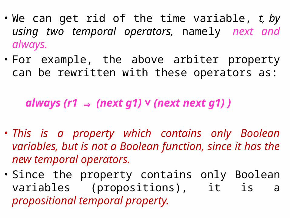
• We can get rid of the time variable, t, by using two temporal operators, namely next and always.

• For example, the above arbiter property can be rewritten with these operators as:

always (r1 (next g1) (next next g1) )⇒ ∨

• This is a property which contains only Boolean variables, but is not a Boolean function, since it has the new temporal operators.

• Since the property contains only Boolean variables (propositions), it is a propositional temporal property.

Properties in SVA language

Design Cycle: Intent creation

Architectural Specification

Executable Specs (CSpec)

Component Specification Document

C, System C

English language document

English language document

Is the intent correct ?

Design intent creation

Design Cycle: Implementation

Component Specification Document

RTL implementation Design Integration

Gate Level Netlist

Transistor level(Schematic)Layout

Mask

Synthesis

Technology Mapping

Implementation Validation (Specification vs RTL)

Verilog, VHDl

Equivalence Checking

Simulator

• A simulator consists of three major components: (i) a front end, (ii) a back end, and (iii) a simulation engine/control• The front end is very much standard for most

simulators and is a function only of the input language.

• The back end performs analysis, optimization, and generation of code to simulate the input circuit, and is the main contributor to a simulator's speed.

Major components of a simulator

• The simulation engine takes in the generated code and computes the behavior.

• The generated code has no direct knowledge of the circuit and can be in any language.

• Simulation control allows the user to interact with the operation of the simulator.

• User can set break points to pause a simulation after a number of time steps, examine variable values, and continue simulation.

Compiler front-end

• The front-end portion of a compiler, consisting of a parser and an elaborator.

• The front end portion of a compiler process the input circuit and builds and internal structure (or representation) of the circuit.

• Parser- creates internal components or data structure

• Elaborator- The elaborator perform module instantiations and constructs a representation of the input circuit by connecting the internal components.

Compiler Backend• Determines the type of the simulator and dictates the

construction of code generation.• For a cycle-based simulator, it performs clock domain

analysis and levelization, whereas • for an FPGA-based hardware simulator, in addition to the

previous analysis it also partitions, places, and routes the circuit into FPGA chips

• There are four classes of generated code: (i) interpreted code, Interpreted code simulator (ii) high-level code, (iii) native code, and Compiled code simulator (iv) emulation code.

Compiler Back-End

Functionality depends on the type of simulator:(i) Compiled code simulator High level code Native code Emulation code

(ii) Interpreted simulator The input circuit is compiled into an intermediate language Can be regarded as a virtual machine

Summary of four types of simulation processes

Interpreted simulation process

The effect of executing the interpreted object code creates the behavior of the circuit. The functions in the interpreted code assign(), invert(), evaluate() are instructions for the interpreted simulator. Note that the stimulus or test bench is compiled with the circuit.

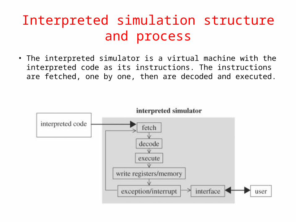
Interpreted simulation structure and process

• The interpreted simulator is a virtual machine with the interpreted code as its instructions. The instructions are fetched, one by one, then are decoded and executed.

Compiled code

The Simulators• Two contrasting architectures: event driven and cycle based.

Event-Driven Simulators• Evaluates a component, only when there is an event at an input or

sensitivity list of the component.

• An event is a change of value in a variable or a signal.

• If an event at a gate input causes one of its outputs to change, all the fan outs of the gate will have to be evaluated.

• This event ripples throughout the circuit until it causes no more events, at which time evaluation stops.

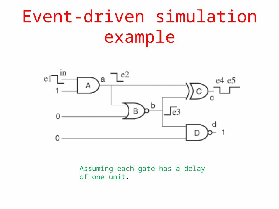
Event-driven simulation example

Assuming each gate has a delay of one unit.

The timing diagram shows five transitions or events, labeled e1, e2, e3, e4, and e5

0

c

b

a

in

Events

time1 2 3 4

e1

e2

e3

e4e5

Timing wheel/event manager• When multiple events occur simultaneously, each of

which causes further events, the simulator, being able to evaluate only one at a time, must schedule an evaluation order of the events.

• Events are stored in an event manager, which sorts them according to event occurrence time.

• When the simulator is at time T, all events that occurred before time T must have been evaluated.

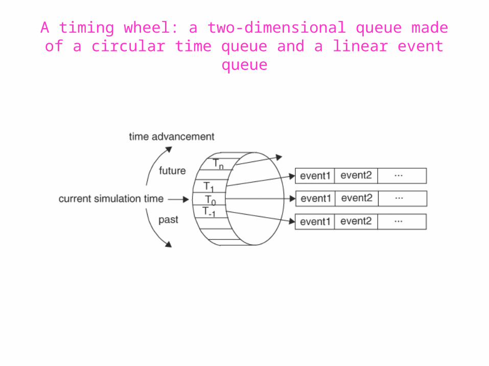
A timing wheel: a two-dimensional queue made of a circular time queue and a linear event queue

Scheduling semantics

• Events at the same time have to be prioritized according to IEEE Verilog standards.

• In Verilog, events at a simulation time are stratified into five layers of events in the following order of processing:

1. Active2. Inactive3. Nonblocking assign update4. Monitor5. Future events.

• Active- Active events at the same simulation time are processed in an arbitrary order. Example, blocking assignment. The processing of all the active events is called a simulation cycle.

• Inactive events are processed only after all active events have been processed. Example zero delay assignment.

• A nonblocking assignment executes in two steps. First it samples the values of the right-side variables. Then it updates the values to the left-side variables. it is executed only after both active and inactive events at the current simulation time have been processed.

• Monitor events are generated by system tasks $monitor and $strobe, which are executed as the last events to capture steady values of variables.

• Finally, events that are to occur in the future are future events.

• All commands display text on the screen during simulation

• $display and $strobe-- display once every time they are executed

• $monitor-- displays every time one of its parameters changes.

• The difference between $display and $strobe is that $strobe displays the parameters at the very end of the current simulation time unit rather than exactly when it is executed.

Here two procedural blocks are scheduled at the same time

always @(posedge clock) begin x = a; end always @(posedge clock) begin x = b; y <= x; y = c; end

Cycle-Based Simulators

• The combinational logic is evaluated at each clock boundary and a gate is evaluated once.

• Therefore, for a circuit to be simulated by a cycle-based simulator, the circuit must have clearly defined clocks and their associated boundaries.

• Consequently, asynchronous circuits and circuits with combinational loops cannot be simulated by cycle-based simulators.

• Furthermore, because only steady states are computed, all delays in the circuit are ignored in cycle-based simulation. All components are assumed to have zero delays.

Cycle-based simulators• In a sequential circuit, every time the FF change; Many events are generated in the CL But only steady state is latched at the next clock edge Evaluation of all intermediate events are wasted

• Cycle based simulators evaluate the combinational logic at each clock boundary

Each gate is evaluated once in each cycle.

• Requirement: the circuit must have clearly defined clocks and their associated boundaries.

Leveling• To compute steady-state values, gates must be evaluated in a

proper order.

• A correct evaluation order for cycle-based simulation must guarantee that a gate is evaluated only after all its inputs have already been evaluated.

• Use topological sort for ordering.

• Do the levelization of the figure given below? Apply the topological sort, based on depth-first search (DFS) starts on primary inputs and FF outputs and returns an ordered list of nodes.

Proper levelization and topological sort for gate evaluation

• Schedule the following RTL code for cycle-based simulation

always @(posedge clk) begin a = b; c <= a; $my PLI (a,b,d); // d is an output$strobe("a=%d,b=%d,c=%d",a,b,c); e = d; end assign x = a << 2; assign y = c; gate gate1(.in1(x), .in2(y),...);

1. a=b; 2. $myPLI (a,b,d); 3. e=d; 4. assign x = a <<2; assign y = c; 5. gate gate1(.in1(x),.in2(y),...); 6. c<=a; 7. $strobe("a=%d,b=%d,c=%d",a,b,c);

Equivalence Checking by BDD

• Binary Decision Diagrams (BDDs) are compact canonical representations of Boolean functions.

• Decision trees based on Shannon’s expansion have been used for propositional reasoning in Artificial Intelligence for many years.

• BDD-based FPV techniques were able to handle as much as 1020 states.

What is a BDD?Given a Boolean function f(x1, . . . , xk) over variables, x1, . . . , xk, we can rewrite f as:

where fx1←1 denotes f with x1 substituted by 1, and fx1←0 denotes f with x1 substituted by 0. This is known as Shannon’s decomposition of f on the variable x1.

Example. make a decision tree for the function f(a, b, c) = c (a b)∧ ∨

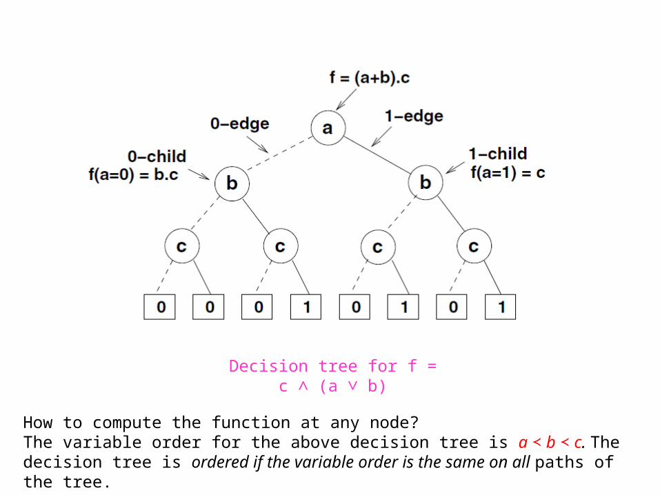
Decision tree for f = c (a b)∧ ∨

How to compute the function at any node?The variable order for the above decision tree is a b c≺ ≺ . The decision tree is ordered if the variable order is the same on all paths of the tree.

Reducing the decision tree to a BDD using self-similarity.

ROBDDTwo rules two get ROBDD from decision tree:

1. Merging ---If two nodes represent the same function, then we merge them. Previous fig. shows the merging of three c-labeled nodes.

2. Elimination---If a node has the same 0-child and 1-child, then that node represents a “don’t care” variable, and is removed.

Formally, it follows from Shannon’s decomposition that f is

independent of xi whenever fxi←0 = fxi←1.

ROBDD• Reduced ordered Binary Decision Diagrams (ROBDD) are canonical in

nature.

• This means that if f and g are two representations of the same Boolean function, then they will have the same ROBDD. Henceforth we will loosely use the term, BDD, to mean a ROBDD.

• Canonicity is a very useful property for formal equivalence checking.

• If we wish to verify whether a given RTL module is an adder, we can extract its logic and create a BDD. We can also create the BDD for the addition function (which is a Boolean function). If the two BDDs are identical, then the RTL correctly implements an adder. Otherwise, the RTL has a bug.

Effect of variable ordering on BDD size. The main limitation here is that the size of a BDD can grow rapidly with the number of variables. The first BDD uses the ordering, a b m n ≺ ≺ ≺

p q≺ ≺ , while the second BDD uses the ordering, a m p b n q.≺ ≺ ≺ ≺ ≺

BDD fo the function f = (a b) (m n) (p q)∧ ∨ ∧ ∨ ∧

Incremental construction of BDDs for a circuit

BDDs for State MachinesBDD representation for a sequential circuit.1. Drop the sequential elements (say flip-flops) from

the circuit to extract the combinational logic.2. For each flip-flop do the following:a) Treat its output, y, as a primary input to the combinational

logic. y represents a present state bit of the state transition relation of the sequential circuit.

b) Treat its input as a primary output of the combinational logic. Call this output y’. Y’ represents the next state variable for y in the state transition relation of the sequential circuit.

3. Build the BDD for the modified combinational logic.

BDDs for transition functions

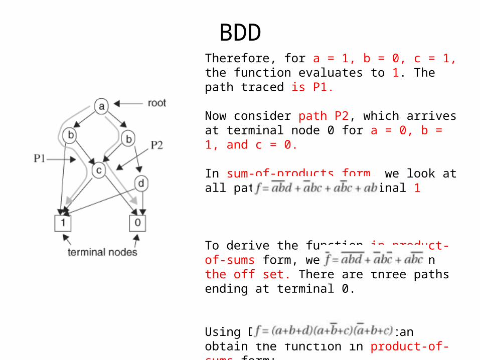
BDDTherefore, for a = 1, b = 0, c = 1, the function evaluates to 1. The path traced is P1.

Now consider path P2, which arrives at terminal node 0 for a = 0, b = 1, and c = 0.

In sum-of-products form, we look at all paths ending at terminal 1

To derive the function in product-of-sums form, we need to work on the off set. There are three paths ending at terminal 0.

Using De Morgan's Law, we can obtain the function in product-of-sums form:

(A, B) BDDs of the same function have different variable ordering

For figure B

Transformations to reduce OBDDs. (A) Merge (B) Eliminate

Whether Two OBDDs represent the same function?

1. There are no nodes A and B such that they share the same 0-node and 1-node.

2. There is no node with two edges that point to the same node.

An OBDD for reduction

Reducing an OBDD. (A) Original BDD (B) Merging of two nodes (C) Eliminating node

References

• A roadmap for formal property verification by Pallab Dasgupta.

• Hardware Design Verification: Simulation and Formal Method-Based Approaches By William K. Lam, Sun Microsystems