Embed Size (px)
Citation preview
University of Southern Queensland
Faculty of Engineering and Surveying
Verification of Simplified Optimum Designs
for Reinforced Concrete Beams
A dissertation submitted by
Nitesh Nitin Prasad
in fulfilment of the requirements of
Courses ENG4111 and ENG4112 Research Project
towards the degree of
Bachelor of Engineering (Civil)
October, 2011
Abstract i
Abstract
Current demand on resources have forced engineering sector to look at more efficient
design and construction methods. Methods that will yield better designs that are cost
effective and puts less demand on decreasing resources. In this dissertation the use of
topology optimisation for the design of concrete beams is investigated. The method
uses topology optimisation to obtain the optimum strut-and-tie model (STM) and
then uses the STM provisions of AS3600:2009 to design the beam. As a control a
similar beam is designed using the conventional design methods and both beams are
tested.
Test results showed that the conventional beam performed better then the optimum
beam and it was concluded that construction methods utilised maybe the reason for
this results. It has been recommended that further research in this area is required
with better construction procedures implemented.

ii Limitation of use
University of Southern Queensland
Faculty of Engineering and Surveying
ENG4111 Research Project Part 1 &
ENG4112 Research Project Part 2
Limitations of Use
The Council of the University of Southern Queensland, its Faculty of Engineering
and Surveying, and the staff of the University of Southern Queensland, do not accept
any responsibility for the truth, accuracy or completeness of material contained
within or associated with this dissertation.
Persons using all or any part of this material do so at their own risk, and not at the
risk of the Council of the University of Southern Queensland, its Faculty of
Engineering and Surveying or the staff of the University of Southern Queensland.
This dissertation reports an educational exercise and has no purpose or validity
beyond this exercise. The sole purpose of the course pair entitled “Research
Project” is to contribute to the overall education within the student's chosen degree
program. This document, the associated hardware, software, drawings, and other
material set out in the associated appendices should not be used for any other
purpose: if they are so used, it is entirely at the risk of the user.
Professor Frank Bullen
Dean
Faculty of Engineering and Surveying

Certification iii
Certification
I certify that the ideas, designs and experimental work, results, analyses and
conclusions set out in this dissertation are entirely my own effort, except where
otherwise indicated and acknowledged.
I further certify that the work is original and has not been previously submitted for
assessment in any other course or institution, except where specifically stated.
Nitesh Nitin Prasad
0050092763:
____________________________
Signature
____________________________
Date

iv Acknowledgement
Acknowledgement
I would like to take this opportunity to thank a few people for their support and
guidance over the past 12 months. Firstly, I would like to thank my project
supervisor, Dr Kazem Ghabraie (USQ) for his continuous support, guidance and
patience. I would like to acknowledge the assistance of USQ technical staff, without
whom the testing phase of the project would have been very difficult. Finally, I
would like to thank my family for their support and words of encouragement when I
needed them.
Without all of your invaluable contribution I would have been able to complete this
dissertation.
Table of contents v
Table of Contents
Abstract ......................................................................................................................... i
Limitations of Use ........................................................................................................ ii
Certification................................................................................................................. iii
Acknowledgement....................................................................................................... iv
Table of Contents ......................................................................................................... v
List of Figures ........................................................................................................... viii
List of Tables............................................................................................................... ix
INTRODUCTION ...................................................................................................... 1
1.1 Background ................................................................................................... 1
1.2 Aims and Objectives ..................................................................................... 2
1.3 Anticipated Potential Outcomes .................................................................... 2
1.4 Methodology ................................................................................................. 3
1.5 Project Resources .......................................................................................... 4
1.6 Risk Assessment and Consequential Effects ................................................. 4
1.7 Project Schedule ............................................................................................ 6
1.8 Dissertation Structure .................................................................................... 7
STRUT-AND-TIE MODELLING ............................................................................ 9
2.1 Introduction ................................................................................................... 9
2.2 Definitions ................................................................................................... 11
2.3 Development of Strut-and-Tie Model ......................................................... 12
2.4 Conventional Approach for Developing Strut-and-Tie Models .................. 13
2.5 Key Components of Strut-and-Tie Models ................................................. 15
2.5.1 Struts ................................................................................................... 15
2.5.2 Ties ....................................................................................................... 17
2.5.3 Nodes ................................................................................................... 17
2.6 Advantages of Using Strut-and-Tie Modelling ........................................... 19
2.7 Limitations of Strut-and-Tie Modelling ...................................................... 19
TOPOLOGY OPTIMISATION TECHNIQUES ................................................. 21
3.1 Introduction ................................................................................................. 21
vi Table of Contents
3.2 Brief History ................................................................................................ 22
3.3 Homogenisation Method ............................................................................. 24
3.3.1 Types of microstructures ..................................................................... 25
3.3.2 Optimally criteria ................................................................................. 26
3.3 SIMP Method .............................................................................................. 27
3.4 Evolutionary Structural Optimisation .......................................................... 28
3.4.1 ESO based on stress level ..................................................................... 28
3.4.2 ESO for stiffness optimisation .................................................................. 28
3.5 Bi-directional Evolutionary Structural Optimisation (BESO) ..................... 29
3.5 Other Available Techniques ........................................................................ 30
METHODOLOGY – DESIGN & TESTING ........................................................ 31
4.1 Design Problem ........................................................................................... 31
4.2 MATLAB Code ........................................................................................... 32
4.2.1 Topology of design problem ................................................................ 33
4.3 Design Procedure ......................................................................................... 34
4.3.1 Conventional method ........................................................................... 34
4.3.2 Strut-and-tie modelling method ........................................................... 36
4.3.3 Concrete mix design ............................................................................. 38
4.4 Finding Optimum Topology of Problems from Literature .......................... 38
4.5 Testing Equipment & Procedure ................................................................. 40
RESULTS .................................................................................................................. 43
5.1 Optimum topology of beam ......................................................................... 43
5.2 Test Results.................................................................................................. 45
5.1.1 Compression test of cylinder samples .................................................. 45
5.1.2 Flexural testing of beams ..................................................................... 48
5.3 Optimum Topology of Problems from Literature ....................................... 51
CONCLUSION & RECOMMENDATIONS ......................................................... 55
6.1 Conclusion ................................................................................................... 55
6.2 Recommendations for Future Work ............................................................ 56
Bibliography ............................................................................................................... 57
Appendix A – Specification ....................................................................................... 63
Appendix B – Topology Optimisation Codes ............................................................ 64
B.1 99 Line Code ............................................................................................... 64
B.2 88 Line Code ............................................................................................... 66
B.3 104 Line Modified Code ............................................................................. 68
Appendix C – Beam Analysis & Calculations ........................................................... 71
C.1 Microstran Output ....................................................................................... 71
C.2 STM design calculations ............................................................................. 73
C.3 Conventional design calculations ................................................................ 77
Appendix D – Beam Reinforcement .......................................................................... 80
Appendix E – Testing Photos ..................................................................................... 82
List of figures viii
List of Figures
Figure 2.1 Geometric and load discontinuities for D-regions .................................... 10
Figure 2.2 Examples of strut-and-tie models ............................................................. 11
Figure 2.3 Types of concrete struts and related stress fields ...................................... 16
Figure 2.4 Bottle-shaped strut .................................................................................... 17
Figure 2.5 Classification of nodes .............................................................................. 18
Figure 2.6 Node types ................................................................................................ 19
Figure 3.1 Structural optimisation categories. ........................................................... 22
Figure 3.2 Microcell with rectangular holes. ............................................................. 25
Figure 3.3 Rank-2 layered (laminate) material. ......................................................... 26
Figure 4.1 Design problem – beam geometry, support and loading conditions. ........ 32
Figure 4.2 Conditions at ultimate moment in a doubly reinforced concrete section. 35
Figure 4.3 Design process, combining topology optimisation and STM. .................. 37
Figure 4.4 Ley beam geometry and loading. (Dimensions are in mm [in.]) .............. 39
Figure 4.5 Schlaich beam geometry and loading. ...................................................... 39
Figure 4.6 SANS (YAW-6206) Compression Testing Machine ................................ 41
Figure 4.7 Specimen set-up on flexure grip ............................................................... 41
Figure 4.8 Beam set-up in compression testing machine ........................................... 42
Figure 5.1 Optimum topology of design problem after 159 iterations ....................... 43
Figure 5.2 Optimisation output at every 20 iteration ................................................. 44
Figure 5.3 Graph of objective function vs iteration ................................................... 45
Figure 5.4 Load versus deflection graph for specimen 1 ........................................... 46
Figure 5.5 Load versus deflection graph for specimen 2 ........................................... 47
Figure 5.6 Load versus deflection graph for specimen 3 ........................................... 47
Figure 5.7 Load versus deflection graph for optimum beam ..................................... 48
Figure 5.8 Crack pattern in optimum beam................................................................ 49
Figure 5.9 Load versus deflection graph for conventional beam ............................... 50
Figure 5.10 Crack pattern in conventional beam ....................................................... 50
Figure 5.11 STM presented by Ley et al (2007) ........................................................ 51
Figure 5.12 Optimum Topology for Ley beam .......................................................... 52
Figure 5.13 STM presented by Schlaich et al (1987) ................................................. 53
Figure 5.14 Optimum topology for Schlaich beam .................................................... 53

List of tables ix
List of Tables
Table 1.1: List of resources and its uses ...................................................................... 4
Table 1.2 Measures of Likelihood ............................................................................... 5
Table 1.3 Measures of Consequence ............................................................................ 5
Table 1.4 Risk analysis matrix ..................................................................................... 5
Table 1.5 Risk summary .............................................................................................. 6
Table 1.6 Project Schedule ........................................................................................... 6
Table 5.1 Cylinder test results .................................................................................... 46

This Page has been left intentionally blank.
Chapter 1
INTRODUCTION
Overview
This chapter gives a brief background of the topic, outlines the aim and objectives,
anticipated potential outcomes, methodology, project resources used, the risk
assessment, project timeline and an outline of the dissertation.
1.1 Background
Reinforced concrete was invented in the mid 1800‟s and there have been enormous
advances in its design and use. Many design techniques and procedures have been
developed over the years, which have been included in design codes and standards.
One of the latest design techniques that is being researched here is topology
optimization. Even though the first paper on topology optimization was published in
1904 (Rozvany 2009), major development in this research field has happened only in
the last few decades. It‟s an extremely rapidly expanding research field, which has
interesting theoretical implications in mathematics, mechanics, multi-physics and
computer science, but also important practical applications by the manufacturing
industries such as car and aerospace (Rozvany 2009). Numerous researchers are
continuingly developing new techniques in this field and some of the more
prominent ones will be discussed in Chapter 3.

2 Introduction
Literature review has found that though there are many papers on topology
optimisation techniques, there is little research being done on its application in
reinforced concrete design and verifying these methods through physical testing.
Liang et al (2002) have used topology optimisation for structural concrete design. It
should be noted that these optimisation techniques are well developed methods that
have been verified through vigorous numerical analysis. Yet, physical testing is
essential as it has been well documented that physical behaviour of reinforced
concrete is hard to model using numerical modelling.
The focus of this project is to optimise the stiffness of a reinforced concrete beam
using one of the topology optimisation techniques and verify this simplified
optimised design through testing. For this project the design domain will be
optimized using a MATLAB code to obtain the optimum layout and then strut and tie
method will be used to design the reinforcement. To compare results, the same beam
will be designed using conventional reinforced concrete design method. Beam
samples for both designs will be constructed and then tested to compare results.
1.2 Aims and Objectives
The aims and specific objectives of this project are as follows:
To verify optimum designs obtained using a simplified linear elastic model for
reinforced concrete.
To test the efficiency and accuracy of the Matlab code.
To be able to provide reinforced concrete designers a simple and effective
method of finding optimum strut-and-tie layout.
1.3 Anticipated Potential Outcomes
Prior to the commencement of this project it was envisaged that the potential
outcomes of this project would include:
Test results comparing well with theoretical values.
Introduction 3
Using verified test results to prepare a method of designing deep beams using
simplified optimization.
Using the data from this project together with other similar projects done by other
USQ students to present a technical paper.
1.4 Methodology
The methodology used to complete this dissertation is described in the following
steps:
1. Research background information relating to topology optimisation, especially
the SIMP (Solid Isotropic Microstructure with Penalisation) method.
A well focused literature review enabled the author to understand the theory
behind the optimization techniques as well as ensure that similar research has not
already been done.
2. Research on concrete beam design by strut-and-tie method. Design methods were
researched including those provided in codes and methods proposed by other
researchers. The design procedure used in this dissertation is explained later in
this dissertation.
3. Select a design problem including beam dimensions.
4. Design the given problem using conventional design methods.
5. Using MATLAB optimisation code determine optimum layout and design using
strut-and-tie method.
6. Prepare test samples for both designs.
7. Test samples and compare results.
8. Conclusions.
9. Recommendations for further research.
4 Introduction
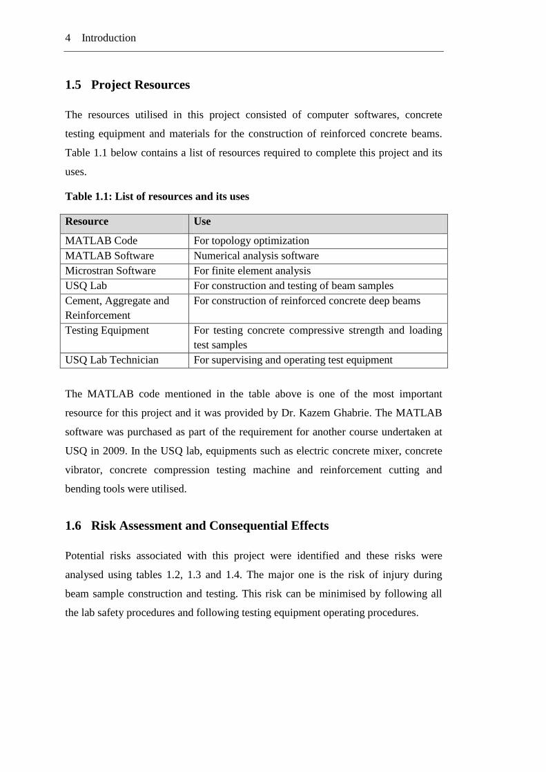
1.5 Project Resources
The resources utilised in this project consisted of computer softwares, concrete
testing equipment and materials for the construction of reinforced concrete beams.
Table 1.1 below contains a list of resources required to complete this project and its
uses.
Table 1.1: List of resources and its uses
Resource Use
MATLAB Code For topology optimization
MATLAB Software Numerical analysis software
Microstran Software For finite element analysis
USQ Lab For construction and testing of beam samples
Cement, Aggregate and
Reinforcement
For construction of reinforced concrete deep beams
Testing Equipment For testing concrete compressive strength and loading
test samples
USQ Lab Technician For supervising and operating test equipment
The MATLAB code mentioned in the table above is one of the most important
resource for this project and it was provided by Dr. Kazem Ghabrie. The MATLAB
software was purchased as part of the requirement for another course undertaken at
USQ in 2009. In the USQ lab, equipments such as electric concrete mixer, concrete
vibrator, concrete compression testing machine and reinforcement cutting and
bending tools were utilised.
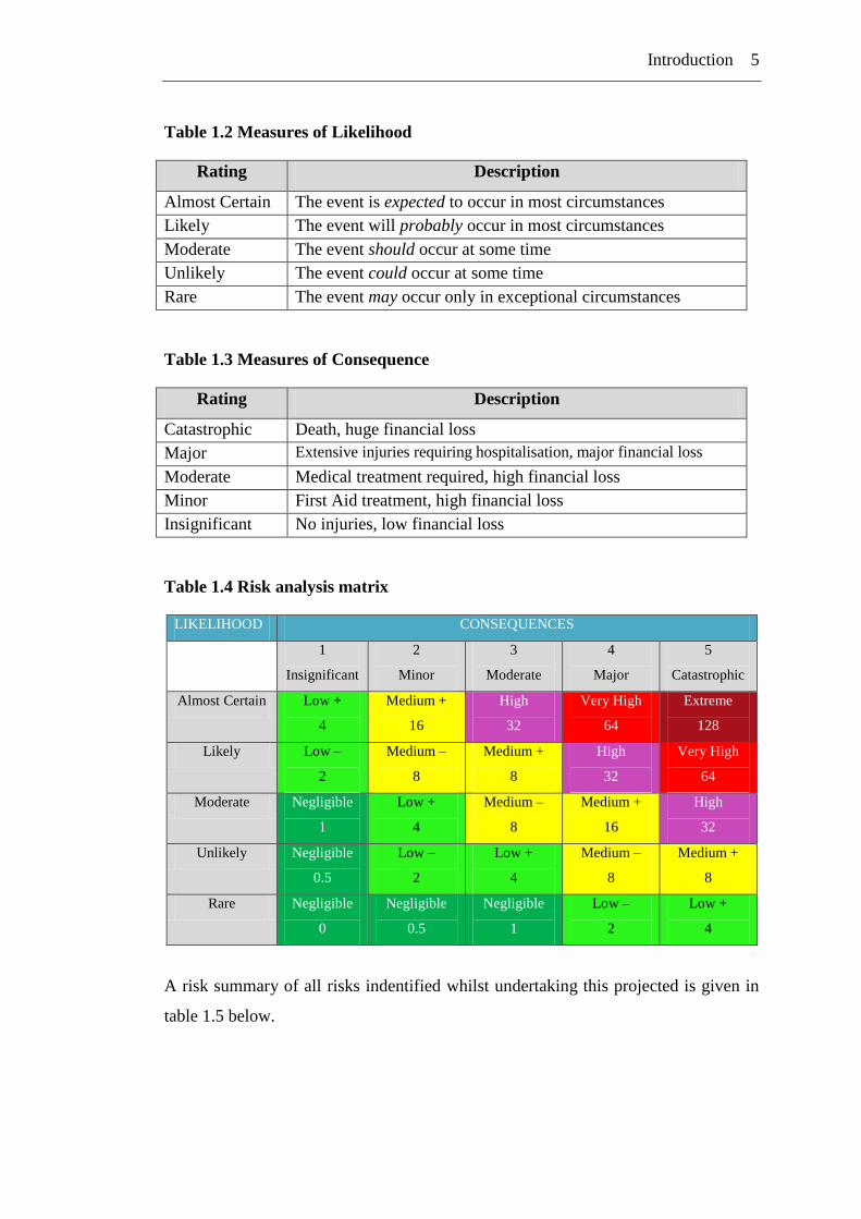
1.6 Risk Assessment and Consequential Effects
Potential risks associated with this project were identified and these risks were
analysed using tables 1.2, 1.3 and 1.4. The major one is the risk of injury during
beam sample construction and testing. This risk can be minimised by following all
the lab safety procedures and following testing equipment operating procedures.
Introduction 5
Table 1.2 Measures of Likelihood
Rating Description
Almost Certain The event is expected to occur in most circumstances
Likely The event will probably occur in most circumstances
Moderate The event should occur at some time
Unlikely The event could occur at some time
Rare The event may occur only in exceptional circumstances
Table 1.3 Measures of Consequence
Rating Description
Catastrophic Death, huge financial loss
Major Extensive injuries requiring hospitalisation, major financial loss
Moderate Medical treatment required, high financial loss
Minor First Aid treatment, high financial loss
Insignificant No injuries, low financial loss
Table 1.4 Risk analysis matrix
LIKELIHOOD CONSEQUENCES
1
Insignificant
2
Minor
3
Moderate
4
Major
5
Catastrophic
Almost Certain Low +
4
Medium +
16
High
32
Very High
64
Extreme
128
Likely Low –
2
Medium –
8
Medium +
8
High
32
Very High
64
Moderate Negligible
1
Low +
4
Medium –
8
Medium +
16
High
32
Unlikely Negligible
0.5
Low –
2
Low +
4
Medium –
8
Medium +
8
Rare Negligible
0
Negligible
0.5
Negligible
1
Low –
2
Low +
4
A risk summary of all risks indentified whilst undertaking this projected is given in
table 1.5 below.

6 Introduction
Table 1.5 Risk summary
Hazard Consequence Likelihood Risk Control
Sharp Tools Moderate Unlikely Low Follow user guide
Electric Tools Moderate Unlikely Low Operate with care
Breaking
Concrete
Moderate Almost Certain High Wear safety glass
The potential consequential effects of this project are minimal. There is no
sustainability issue that needs to be considered for this project. The ethical issues
related to this project include firstly crediting other researchers where it is due for
using their ideas and secondly, responsibly conducting and reporting this project as
the results could be used by designers and other researchers who will have an
expectation that this project has been done diligently. The safety issues while
undertaking this project have been discussed above. The safety issues after the
completion of the project include incorrect use of project results. That is, designers
incorrectly or inappropriately using the results of this project to design reinforced
concrete beams. If the results of this project are not properly and independently
verified then it should not be used by designers.
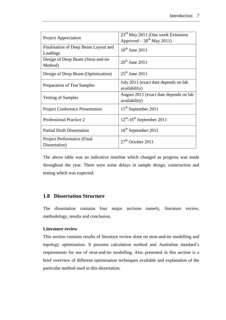
1.7 Project Schedule
As means to track progress and manage time for this project a schedule was prepared
for completing various sections of this dissertation and requirements of ENG4111
and ENG4112 and it is tabulated in table 1.6 below.
Table 1.6 Project Schedule
Phase of Work Completion Date
Project Proposal 9th
March 2011
Project Specification 22nd
March 2011
Literature Review 30th
June 2011
Introduction 7
Project Appreciation 23
rd May 2011 (One week Extension
Approved – 30th
May 2011)
Finalisation of Deep Beam Layout and
Loadings 10
th June 2011
Design of Deep Beam (Strut-and-tie
Method) 20
th June 2011
Design of Deep Beam (Optimization) 25th
June 2011
Preparation of Test Samples July 2011 (exact date depends on lab
availability)
Testing of Samples August 2011 (exact date depends on lab
availability)
Project Conference Presentation 11th
September 2011
Professional Practice 2 12th
-16th
September 2011
Partial Draft Dissertation 16th
September 2011
Project Performance (Final
Dissertation) 27
th October 2011
The above table was an indicative timeline which changed as progress was made
throughout the year. There were some delays in sample design, construction and
testing which was expected.
1.8 Dissertation Structure
The dissertation contains four major sections namely, literature review,
methodology, results and conclusion.
Literature review
This section contains results of literature review done on strut-and-tie modelling and
topology optimisation. It presents calculation method and Australian standard‟s
requirements for use of strut-and-tie modelling. Also presented in this section is a
brief overview of different optimisation techniques available and explanation of the
particular method used in this dissertation.

8 Introduction
Methodology
Presented in this section are the details of the Matlab code used for optimisation. The
sample problem chosen for this dissertation is presented, together with its design
method and calculations. A brief explanation of the testing method and equipment
used is also given.
Results
In this section the results from testing and numerical analysis is discussed and
compared with each other.
Conclusion
From the results obtained conclusions are drawn and brief explanation of the results
is given. Recommendations for future works are also made in this section.
Chapter 2
STRUT-AND-TIE MODELLING
Overview
This chapter summaries the literature review done on the strut-and-tie modelling. It
includes the history, development methods, key components, advantages and
limitations of the strut-and-tie modelling.
2.1 Introduction
Reinforced concrete beam theory is based on equilibrium and the constitutive
behaviour of the materials, steel and concrete. Particularly important is the
assumption that strain varies linearly through the depth of a member and that, as a
result plane sections remain plane. St. Venant‟s principle validated this assumption
by stating that strains around load or member cross section discontinuity vary in an
approximately linear fashion at distance greater than or equal to the greatest cross
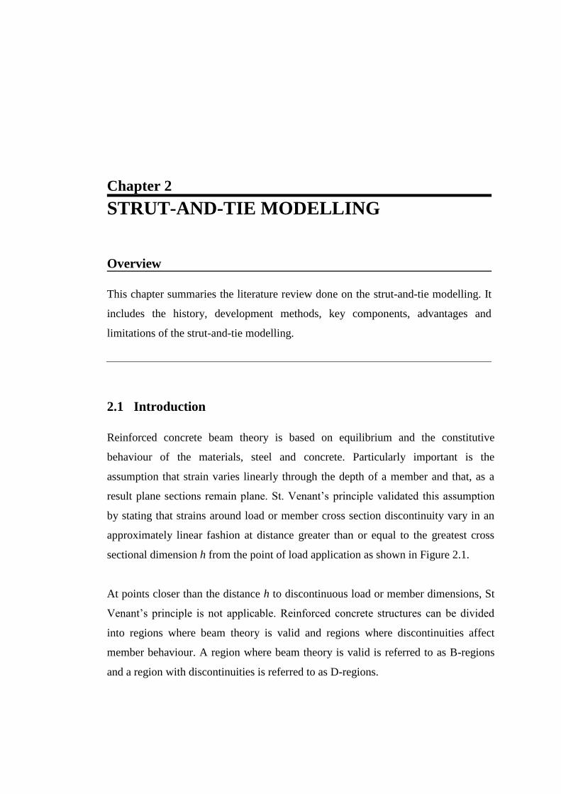
sectional dimension h from the point of load application as shown in Figure 2.1.
At points closer than the distance h to discontinuous load or member dimensions, St
Venant‟s principle is not applicable. Reinforced concrete structures can be divided
into regions where beam theory is valid and regions where discontinuities affect
member behaviour. A region where beam theory is valid is referred to as B-regions
and a region with discontinuities is referred to as D-regions.
10 Strut-and-tie modelling
Figure 2.1 Geometric and load discontinuities for D-regions
(Source: Nilson et al, 2004)
When the concrete is elastic and uncracked, the stresses in D-regions can be
determined using finite element analysis and elastic theory. After concrete cracks the
strain field is disrupted and internal forces are redistributed. The internal force can be
represented by a statically determinate truss known as the strut-and-tie model, which
(a) Geometric discontinuities
(b) Loading discontinuities
Strut-and-tie modelling 11
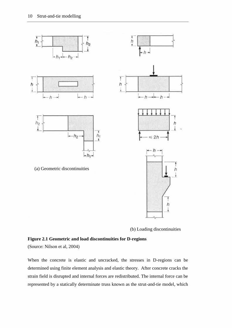
allows the complex problem to be simplified. Figure 2.2 shows examples of strut-
and-tie model in typical reinforced concrete members.
Figure 2.2 Examples of strut-and-tie models
(Source: Warner et al, 2007)
2.2 Definitions
The following terms are used in this section (Warner et al, 2007):
B-region – A portion of a structure in which the Bernoulli-Euler assumption that
plane sections remain plane can be applied.
Discontinuity – An abrupt change in member‟s geometry or loading.
D-region – The portion of a member within a distance equal to the member depth h
from a force discontinuity or a geometry discontinuity. In D-regions Bernoulli-Euler
assumption is not valid after the concrete cracks.
Node – A point in a strut-and-tie model where the axes of the struts, ties and
concentrated forces acting on the joint intersect.
(a) Deep beam
(b) Corbel
(c) Dapped connection (d) Prestressing anchorage
12 Strut-and-tie modelling
Nodal zone – The volume of concrete surrounding a node that transfers strut-and-tie
forces through the node.
Strut – A compressive member in a strut-and-tie model. A strut represents the
resultant of a parallel or fan-shaped compressive field.
Bottle-shaped strut – A strut that is wider at mid-length than at its ends.
Strut-and-tie model – A truss model of a structural member, made up of struts and
ties connected at nodes that is capable of transforming the factored loads to the
supports.
Tie – A tension member in a strut-and-tie model.
2.3 Development of Strut-and-Tie Model
Strut-and-tie modelling has increased in popularity since it was promoted by Marti
(1985a, 1985b) and Schlaich et al (1987). Though much development of strut-and-tie
method occurred after the ground breaking paper by Schlaich et al (1987), the
authors of that paper acknowledge that they were not the first to present the idea of
using truss analogy to design structural concrete. According to them it was at the turn
of the last century when Ritter and Morsch introduced the truss analogy.
Ritter found that a reinforced concrete beam after cracking due to diagonal tensile
stresses could be idealized as a parallel chord truss with compressive diagonals
inclined at 45o
with respect to the longitudinal axis of the beam. Morsch (1920,
1922) extended the truss models to the design of reinforced concrete members under
torsion (Liang, 2005). This method was later refined and expanded by Leonhardt,
Rusch, Kupfer and others until Thurlimann‟s Zurich school, with Marti and Mueller,
created its scientific basis for a rational application in tracing the concept back to the
theory of plasticity.
The standard truss model was developed to be used for designing regions of concrete
structure where the Bernoulli hypothesis of plane strain distribution was assumed to
be valid. But this model could not be applied in regions where the strain distribution
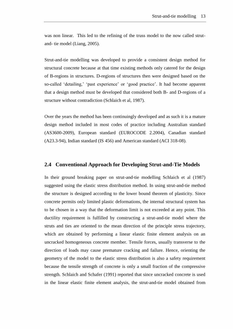
Strut-and-tie modelling 13
was non linear. This led to the refining of the truss model to the now called strut-
and- tie model (Liang, 2005).
Strut-and-tie modelling was developed to provide a consistent design method for
structural concrete because at that time existing methods only catered for the design
of B-regions in structures. D-regions of structures then were designed based on the
so-called „detailing,‟ „past experience‟ or „good practice‟. It had become apparent
that a design method must be developed that considered both B- and D-regions of a
structure without contradiction (Schlaich et al, 1987).
Over the years the method has been continuingly developed and as such it is a mature
design method included in most codes of practice including Australian standard
(AS3600-2009), European standard (EUROCODE 2.2004), Canadian standard
(A23.3-94), Indian standard (IS 456) and American standard (ACI 318-08).
2.4 Conventional Approach for Developing Strut-and-Tie Models
In their ground breaking paper on strut-and-tie modelling Schlaich et al (1987)
suggested using the elastic stress distribution method. In using strut-and-tie method
the structure is designed according to the lower bound theorem of plasticity. Since
concrete permits only limited plastic deformations, the internal structural system has
to be chosen in a way that the deformation limit is not exceeded at any point. This
ductility requirement is fulfilled by constructing a strut-and-tie model where the
struts and ties are oriented to the mean direction of the principle stress trajectory,
which are obtained by performing a linear elastic finite element analysis on an
uncracked homogeneous concrete member. Tensile forces, usually transverse to the
direction of loads may cause premature cracking and failure. Hence, orienting the
geometry of the model to the elastic stress distribution is also a safety requirement
because the tensile strength of concrete is only a small fraction of the compressive
strength. Schlaich and Schafer (1991) reported that since uncracked concrete is used
in the linear elastic finite element analysis, the strut-and-tie model obtained from
14 Strut-and-tie modelling
elastic stress distribution method may differ from the actual load transfer mechanism
at the ultimate limit states.
The load path method can also be used to develop strut-and-tie models in structural
concrete. The first step in this method is to ensure that the external forces are in
equilibrium, that is, the loads and support reactions. The load paths are then traced
using the corresponding stress diagrams. After tracing load paths in the direction of
loads, further struts and ties must be added for transverse equilibrium between nodes.
In selecting the model, it is helpful to realise that loads try to use the path with the
least forces and deformations. Since reinforced ties are much more deformable than
concrete struts, the model with the least and shorted ties are the best (Schlaich et al,
1987). This criterion can be formulated as follows;
(2.1)
where:
Fi = force in strut or tie i
li = length of member i
εmi = mean strain in member i
This equation is derived from the principle of minimum strain energy for linear
elastic behaviour of struts and ties.
For complicated cases Schlaich et al (1987) recommended using a combination of
finite element analysis and load path method for developing new strut-and-tie
models. However, it is difficult to find the optimum models in structural concrete
members with complex loading and geometry using these conventional methods,
which usually involve a trial and error process or requires some prior experience in
modelling.
Marti (1985) realized the limitations of conventional methods for developing strut-
and-tie models and suggested that there is a potential for applying iterative computer
programs with graphical input and output routines which could replace the traditional
Strut-and-tie modelling 15
drawing board method for developing strut-and-tie models. In Chapter 3 such a
method is presented.
2.5 Key Components of Strut-and-Tie Models
Strut-and-tie modelling is considered the basic tool in the design and detailing of
structural concrete under bending, shear and torsion. The designer specifies a load
path and then designs and details the structure such that this load path is sufficiently
strong to carry the applied loads. The loads applied to the structural concrete member
are transferred through a set of compressive stress fields that are distributed and
interconnected by tension ties. The compression stress fields are idealised using
compression members called struts while tensile stress fields are idealised using
tension members called ties. Tension ties can be reinforcing steel bars or prestressed
tendons or concrete in tension. Concrete‟s tensile strength is considerably less than
its compressive strength and normally concrete‟s tensile resistance is ignored.
2.5.1 Struts
A strut is an internal compression member. It may have a prismatic, fan or bottle
shape as shown in Figure 2.3. Prismatic shape is an idealised representation of fan or
bottle shaped struts. The dimensions of the cross section of the strut are established
by the contact area between the strut and the nodal zone.
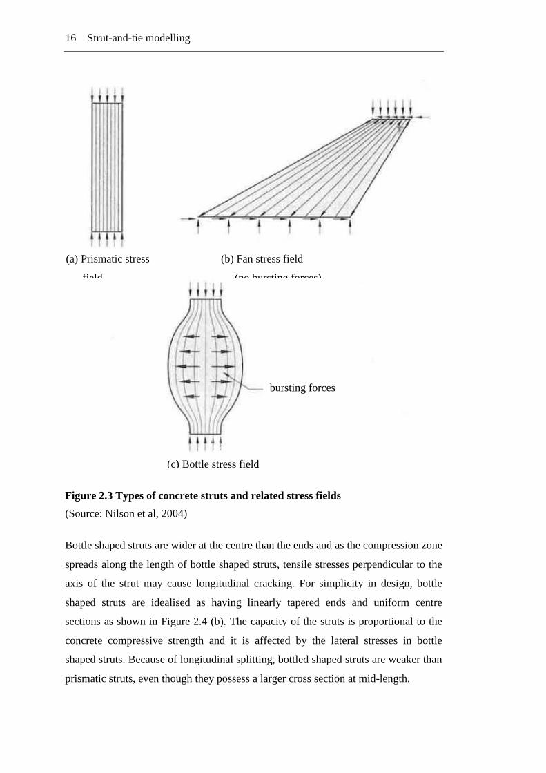
16 Strut-and-tie modelling
Figure 2.3 Types of concrete struts and related stress fields
(Source: Nilson et al, 2004)
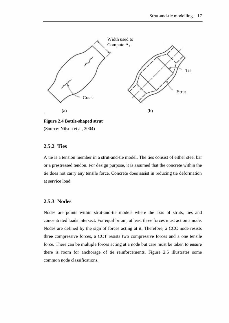
Bottle shaped struts are wider at the centre than the ends and as the compression zone
spreads along the length of bottle shaped struts, tensile stresses perpendicular to the
axis of the strut may cause longitudinal cracking. For simplicity in design, bottle
shaped struts are idealised as having linearly tapered ends and uniform centre
sections as shown in Figure 2.4 (b). The capacity of the struts is proportional to the
concrete compressive strength and it is affected by the lateral stresses in bottle
shaped struts. Because of longitudinal splitting, bottled shaped struts are weaker than
prismatic struts, even though they possess a larger cross section at mid-length.
(a) Prismatic stress
field
(b) Fan stress field
(no bursting forces)
bursting forces
(c) Bottle stress field
Strut-and-tie modelling 17
Figure 2.4 Bottle-shaped strut
(Source: Nilson et al, 2004)
2.5.2 Ties
A tie is a tension member in a strut-and-tie model. The ties consist of either steel bar
or a prestressed tendon. For design purpose, it is assumed that the concrete within the
tie does not carry any tensile force. Concrete does assist in reducing tie deformation
at service load.
2.5.3 Nodes
Nodes are points within strut-and-tie models where the axis of struts, ties and
concentrated loads intersect. For equilibrium, at least three forces must act on a node.
Nodes are defined by the sign of forces acting at it. Therefore, a CCC node resists
three compressive forces, a CCT resists two compressive forces and a one tensile
force. There can be multiple forces acting at a node but care must be taken to ensure
there is room for anchorage of tie reinforcements. Figure 2.5 illustrates some
common node classifications.
(a) (b)
Width used to
Compute Ac
Crack
Strut
Tie

18 Strut-and-tie modelling
Figure 2.5 Classification of nodes
(Source: Nilson et al, 2004)
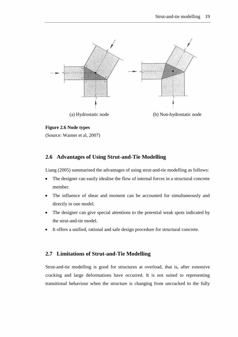
Both tensile and compressive forces place nodes in compression because tensile
forces are treated as if they pass through the node and apply compression in the
anchorage face. There are two types of nodes, non hydrostatic and hydrostatic nodes.
A node is hydrostatic if all members are at right angles to the adjacent node face, as
shown in Figure 2.6 (a). If one or more of the members enter the node at an angle
other than right angle, the node is non hydrostatic as shown in Figure 2.6 (b) (Warner
et al, 2007).
(a) C-C-C node (b) C-C-T node
(c) C-T-T node (d) T-T-T node
Strut-and-tie modelling 19
Figure 2.6 Node types
(Source: Warner et al, 2007)
2.6 Advantages of Using Strut-and-Tie Modelling
Liang (2005) summarised the advantages of using strut-and-tie modelling as follows:
The designer can easily idealise the flow of internal forces in a structural concrete
member.
The influence of shear and moment can be accounted for simultaneously and
directly in one model.
The designer can give special attentions to the potential weak spots indicated by
the strut-and-tie model.
It offers a unified, rational and safe design procedure for structural concrete.
2.7 Limitations of Strut-and-Tie Modelling
Strut-and-tie modelling is good for structures at overload, that is, after extensive
cracking and large deformations have occurred. It is not suited to representing
transitional behaviour when the structure is changing from uncracked to the fully
(a) Hydrostatic node (b) Non-hydrostatic node

20 Strut-and-tie modelling
cracked condition (Warner et al, 2007). The strut-and-tie model is a conservative,
design approach which means that it is almost always over designed.
There is no single design solution and the designer has the flexibility to choose the
shape and dimensions of the strut-and-tie model. This fact requires the designer to
have some experience in the use of strut-and-tie modelling so that they can choose an
effective model.
The strut-and-tie modelling offers the designer the flexibility to focus on
performance design while also providing a safe design. Different performance
criteria may be achieved with strut-and-tie modelling, however, the ultimate failure
mode and load cannot be predicted by strut-and-tie modelling.
Chapter 3
TOPOLOGY OPTIMISATION TECHNIQUES
Overview
This chapter summaries the literature review done on topology optimisation
techniques. It includes the history, uses, and types of topology optimisation
techniques available.
3.1 Introduction
The efficient use of material is important in many different settings. For example, the
aerospace industry and the automotive industry use sizing and shape optimisation to
design structures and mechanical elements. Efficient use of materials is not only cost
effective but it helps to maintain a sustainable future.
Topology optimisation involves the determination of features such as the number,
location and shape of holes and the connectivity of the domain (Bendsoe and
Sigmund, 2003). This method distributes the specified amount of material in a
design domain depending on the design variables. The optimisation of geometry and
topology has great impact on the performance of structures such as increasing the
structures stiffness. Topology optimisation is the newest of different types‟ of
structural optimisation techniques available, which include shape and size
optimisation. In shape optimisation the overall layout of the members is known but
the best shape is required, where as in size optimisation the optimum member
22 Topology optimisation techniques
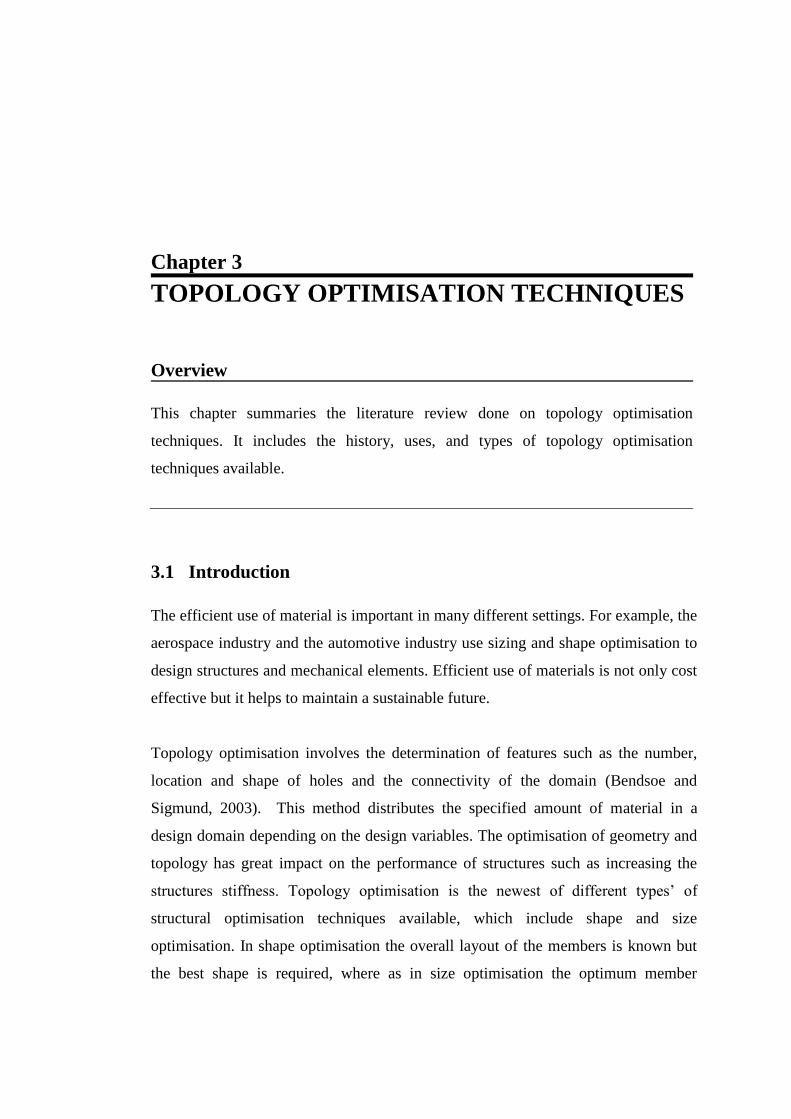
dimensions is determined. Figure 3.1 shows these three structural optimisation
categories.
Figure 3.7 Structural optimisation categories.
a) Topology optimisation; b) Shape optimisation; c) Size optimisation. The initial
problems are shown at the left and the optimal solutions are shown at the right.
(Source: Ghabrie, 2010)
Topology optimisation is used for optimising the stiffness of the design problem in
this dissertation hence shape and size optimisation will not be discussed further here.
3.2 Brief History
There are two broad classes of techniques that can be applied to optimize shape and
topology of a structural system:
Discrete optimization of the structural system.
Continuum optimization of the structural system.
(a)
(b)
(c)
Topology optimisation techniques 23
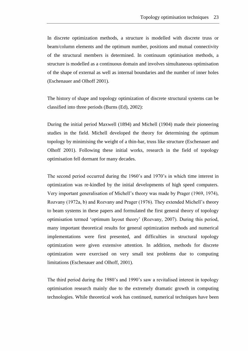
In discrete optimization methods, a structure is modelled with discrete truss or
beam/column elements and the optimum number, positions and mutual connectivity
of the structural members is determined. In continuum optimisation methods, a
structure is modelled as a continuous domain and involves simultaneous optimisation
of the shape of external as well as internal boundaries and the number of inner holes
(Eschenauer and Olhoff 2001).
The history of shape and topology optimization of discrete structural systems can be
classified into three periods (Burns (Ed), 2002):
During the initial period Maxwell (1894) and Michell (1904) made their pioneering
studies in the field. Michell developed the theory for determining the optimum
topology by minimising the weight of a thin-bar, truss like structure (Eschenauer and
Olhoff 2001). Following these initial works, research in the field of topology
optimisation fell dormant for many decades.
The second period occurred during the 1960‟s and 1970‟s in which time interest in
optimization was re-kindled by the initial developments of high speed computers.
Very important generalisation of Michell‟s theory was made by Prager (1969, 1974),
Rozvany (1972a, b) and Rozvany and Prager (1976). They extended Michell‟s theory
to beam systems in these papers and formulated the first general theory of topology
optimisation termed „optimum layout theory‟ (Rozvany, 2007). During this period,
many important theoretical results for general optimization methods and numerical
implementations were first presented, and difficulties in structural topology
optimization were given extensive attention. In addition, methods for discrete
optimization were exercised on very small test problems due to computing
limitations (Eschenauer and Olhoff, 2001).
The third period during the 1980‟s and 1990‟s saw a revitalised interest in topology
optimisation research mainly due to the extremely dramatic growth in computing
technologies. While theoretical work has continued, numerical techniques have been
24 Topology optimisation techniques
further refined, developed and applied to larger scale, more realistic structures
(Eschenauer and Olhoff, 2001).
Also in this third period continuum structural topology optimization techniques were
developed. It was first proposed by Cheng and Olhoff (1981) and some further
research was done by Kohn and Strang (1986). First practical approach to topology
optimisation was demonstrated by Bendsoe and Kikuchi (1988) utilising a
homogenization approach. Flowing this work, Xie and Steven (1993) proposed a
simple finite element based topology optimisation technique, in which inefficient
elements in the design domain is gradually removed based on some optimality
criteria. These two works attracted numerous researchers to the field and it has seen
major development of the theory, techniques and its application in industry. The
great potential of topology optimisation in Civil engineering has not yet been realised
but there is growing consensus to further research into this area.
3.3 Homogenisation Method
In their ground breaking paper, Bendsoe and Kikuchi (1988) presented the
homogenisation method. Subsequent research on the field of structural topology
optimisation has been on the basis of their work. The homogenisation method works
on the basis of replacing materials in a composite domain with a kind of equivalent
material model. This is done because “even with the help of high-speed modern
computers, the analysis of the boundary value problems consisting of composite
media with a large number of heterogeneities is extremely difficult” (Hassani and
Hinton 1998a). Such a procedure is called homogenisation. It is assumed that the
design domain is made of periodic microstructures, hence this type of materials are
called composites with periodic microstructures.
The above mentioned microstructures can be introduced in the design domain using
two methods; the rank laminate composite method or the microcells with internal
voids (Hassani and Hinton, 1998b). The geometric parameters of these
Topology optimisation techniques 25
microstructures are the design variables and by adjusting them it is possible that the
void area inside the microstructure remains a void or changes to solid.
3.3.1 Types of microstructures
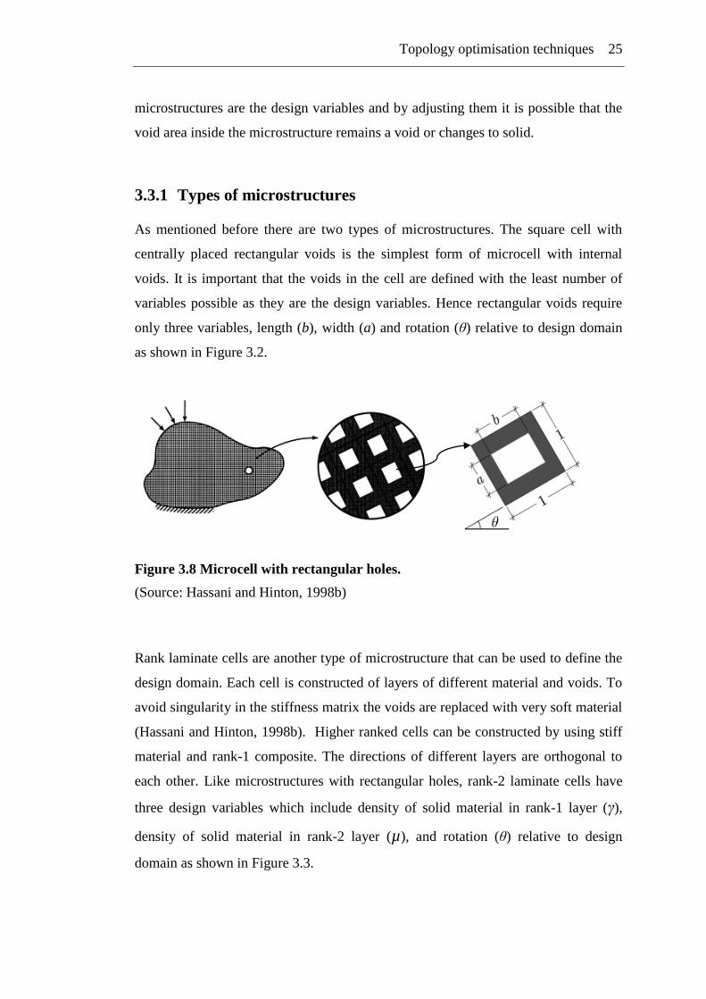
As mentioned before there are two types of microstructures. The square cell with
centrally placed rectangular voids is the simplest form of microcell with internal
voids. It is important that the voids in the cell are defined with the least number of
variables possible as they are the design variables. Hence rectangular voids require
only three variables, length (b), width (a) and rotation (θ) relative to design domain
as shown in Figure 3.2.
Figure 3.8 Microcell with rectangular holes.
(Source: Hassani and Hinton, 1998b)
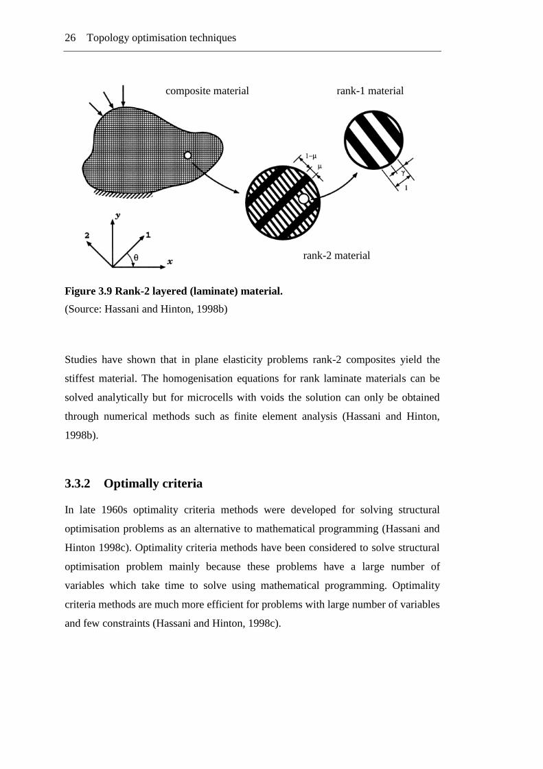
Rank laminate cells are another type of microstructure that can be used to define the
design domain. Each cell is constructed of layers of different material and voids. To
avoid singularity in the stiffness matrix the voids are replaced with very soft material
(Hassani and Hinton, 1998b). Higher ranked cells can be constructed by using stiff
material and rank-1 composite. The directions of different layers are orthogonal to
each other. Like microstructures with rectangular holes, rank-2 laminate cells have
three design variables which include density of solid material in rank-1 layer (γ),
density of solid material in rank-2 layer (µ), and rotation (θ) relative to design
domain as shown in Figure 3.3.
26 Topology optimisation techniques
Figure 3.9 Rank-2 layered (laminate) material.
(Source: Hassani and Hinton, 1998b)
Studies have shown that in plane elasticity problems rank-2 composites yield the
stiffest material. The homogenisation equations for rank laminate materials can be
solved analytically but for microcells with voids the solution can only be obtained
through numerical methods such as finite element analysis (Hassani and Hinton,
1998b).
3.3.2 Optimally criteria
In late 1960s optimality criteria methods were developed for solving structural
optimisation problems as an alternative to mathematical programming (Hassani and
Hinton 1998c). Optimality criteria methods have been considered to solve structural
optimisation problem mainly because these problems have a large number of
variables which take time to solve using mathematical programming. Optimality
criteria methods are much more efficient for problems with large number of variables
and few constraints (Hassani and Hinton, 1998c).
composite material rank-1 material
rank-2 material
Topology optimisation techniques 27
3.3 SIMP Method
The SIMP (Solid Isotropic Microstructures with Penalisation) was proposed by
Bendsoe (1989) which he called the direct approach method. Rozvany introduced the
term „SIMP‟ in 1992, which was not accepted by the research schools until recently
(Rozvany, 2001). It is also known as the „power law‟ method (Rovany, 2001). The
relationship between the elasticity tensor and the density of the base material is
referred to as material interpolation scheme (Bendsoe and Sigmund, 1999).
The basic concept of SIMP method is that „grey‟ elements are penalised and removed
from the domain to obtain a black (ρ = 1) and white (ρ = 0) topology. That is any
element that has density within 0 < ρ < 1 is removed from the design domain. The
first step in this method is to choose a suitable design domain or reference domain
which allows the definition of surface tractions and other boundary conditions
(Bendsoe, 1989). It is assumed that the domain is made of an artificial material and
its density can be related to structures stiffness by the following power law (Bendsoe
and Sigmund, 1999):
(3.1)
where: s = stiffness of structure
ρ = density of artificial material
p > 1, penalty parameter
The density variable is within the limits 0 ≤ ρ ≤ 1 but to avoid singular finite element
matrix a small lower bound, 0 < ρmin ≤ ρ is imposed. As the penalty parameter is
increased the element with intermediate densities is penalised as it‟s structurally less
effective and doesn‟t contribute the structural stiffness of the design domain. The
algorithm will redistribute the material of given volume within the design domain
(Burns (Ed), 2005). A penalty parameter of p ≥ 3 should be used to obtain a good
topology.
28 Topology optimisation techniques
The advantage of SIMP method over other similar methods is that it only requires
one variable per element in the ground structure and also it requires no
homogenisation.
3.4 Evolutionary Structural Optimisation
The Evolutionary Structural Optimisation (ESO) method was proposed by Xie and
Steven (1993). The basic idea of the method is that inefficient elements are removed
from the design domain based on a material removal criterion. Such a criterion
function or parameter value is calculated for each element and in each iteration some
elements with the lowest criterion value that do not meet the minimum criterion set
are eliminated (Rozvany, 2001). By progressively removing such elements the
structure will evolve towards an optimum. This method totally removes inefficient
elements and as such is sometimes referred to as the „hard kill‟ method.
3.4.1 ESO based on stress level
The stress level of the elements in the design domain can be found using finite
element analysis and low stress levels can be interpreted as underutilized materials.
This concept has been used in this method to remove underutilized materials with
stress levels below a threshold value. When all the elements below the threshold
values have been removed the threshold value is increased and the iteration started
again. This procedure of increasing the threshold value continues until a desired
optimum is obtained, for example, when there is no material in the final structure that
has a stress level below 25% of the maximum stress (Huang and Xie, 2010).
3.4.2 ESO for stiffness optimisation
In the design of structures such as building and bridges the stiffness is one of the key
factors to consider. Keeping this in mind the compliance based method was
developed. Mean compliance is the inverse measure of the overall stiffness of the
structure (Huang and Xie, 2010). That is by minimising the compliance, the stiffness
Topology optimisation techniques 29
in maximised. The compliance can be defined by the total strain energy of the
structure or the external work done by the loads on the structure.
The element with the lowest sensitivity number is removed in each iteration. The
sensitivity number is an approximation of the change in the compliance as a result of
removing an element. At each iteration the number of elements removed is restricted
by the element removal ratio which is the ratio of the number of elements removed in
each iteration to the total number of initial or current elements.
According to Rozvany (2001) ESO is an inappropriate name for this method as
„evolutionary‟ means a genetic algorithm whereas „optimisation‟ means to find
optimum solutions. He proposed the name SERA (Sequential Element Rejections
and Admissions) for such methods.
3.5 Bi-directional Evolutionary Structural Optimisation (BESO)
Two major deficiencies present in early versions of ESO method was solution time
and uniqueness (Querin et al, 1998). Since elements were only removed in the ESO
method, it was questioned if the method ensured that it was not a local optimum
solution that was obtained and could the elements removed, be returned. The „Bi-
directional Evolutionary Structural Optimisation‟ method presented by Querin et al
(1998) provided an improved version of the ESO algorithm. The improved method
was able to remove inefficient material to eliminate low stress as well as add
materials to efficient areas to alleviate high stress.
The element efficiency in BESO is measured the same way as in ESO but the adding
and removing uses a different procedure. A control parameter named „Inclusion
Ratio‟ is used to control the amount of material that is added. When no more
elements is removed or added that is at steady state, the inclusion ratio is decreased
and the rejection ratio is increased.
30 Topology optimisation techniques
3.5 Other Available Techniques
There are other techniques available that are extension of the methods outlined
above. Some of them are briefly described below.
BESO utilising SIMP
This method incorporates the BESO method with the SIMP method for determining
the sensitivity number of the elements. See Huang and Xie (2010) for further details.
Performance-base optimisation (PBO)
The PBO method combines the topology and sizing optimisation into a single
scheme to achieve the optimal topology and thickness design of continuum
structures. The performance of the structure is the objective criteria for the method
that is it uses realistic performance criteria. These performance criteria include
structures stiffness, strain, shear, etc. See Liang (2005) for further details.
Chapter 4
METHODOLOGY – DESIGN & TESTING
Overview
This chapter outlines the design and testing methods used in this dissertation. It
includes brief design procedure of strut-and-tie (STM) modelling, summary of
requirements of AS3600:2009 for STM methods and conventional beam design
method. The testing procedure used is summarised including brief description of
testing equipment used and its functions.
4.1 Design Problem
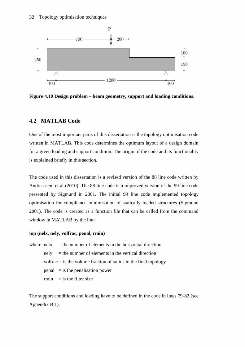
Before explaining the methodology used in this dissertation, it‟s best to present the
design problem first. Figure 4.1 shows the beam geometry, the support conditions
and loading. As shown the beam is 1400mm long with a depth of 250mm. The width
of the beam is 100mm. On the right end, for a length of 500mm the beam depth has
been reduced to only 150mm. This was done to create a D-region (see chapter 2 for
definition) in the beam. The beam supports have been placed 100mm from each end
so that there is some bearing for the supports as it‟s obvious that the beam cannot be
supported at the edge of the beam. Hence the effective beam span is only 1200mm. A
single point load at the mid-span of the beam is applied which makes the design
problem quite simple and also makes setting up the experiment fairly simple.
32 Topology optimisation techniques
Figure 4.10 Design problem – beam geometry, support and loading conditions.
4.2 MATLAB Code
One of the most important parts of this dissertation is the topology optimisation code
written in MATLAB. This code determines the optimum layout of a design domain
for a given loading and support condition. The origin of the code and its functionality
is explained briefly in this section.
The code used in this dissertation is a revised version of the 88 line code written by
Andreassem et al (2010). The 88 line code is a improved version of the 99 line code
presented by Sigmund in 2001. The initial 99 line code implemented topology
optimisation for compliance minimisation of statically loaded structures (Sigmund
2001). The code is created as a function file that can be called from the command
window in MATLAB by the line:
top (nelx, nely, volfrac, penal, rmin)
where: nelx = the number of elements in the horizontal direction
nely = the number of elements in the vertical direction
volfrac = is the volume fraction of solids in the final topology
penal = is the penalisation power
rmin = is the filter size
The support conditions and loading have to be defined in the code in lines 79-82 (see
Appendix B.1).
P
Topology optimisation techniques 33
The improvement in the 88 line code is that the original sensitivity filter is extended
by a density filter and the efficiency has been considerably improved by
preallocating arrays and vectorizing loops. The code is called up in MATLAB in a
similar manner to the 99 line code but with the line:
top (nelx, nely, volfrac, penal, rmin, ft)
where the additional argument ft specifies whether sensitivity filter (ft = 1) or density
filter (ft = 2) is used. When sensitivity filter is used the topology obtained is identical
to that obtained by the 99 line code. Readers are referred to papers by Sigmund
(2001) and Andreassen et al (2010) for a comprehensive detail of the two codes.
4.2.1 Topology of design problem
As mentioned earlier the 88 line code was revised for use in this dissertation. The
noticeable changes were the removal of the density filter and hence the argument ft
was no longer needed. A number of lines were added to improve the output and the
new code:
shows initial topology and prints it to the file T0000.pdf;
prints the topology after every 10 iterations to the files T0010.pdf, T0020.pdf,
T0030.pdf, ...;
stores the values of the objective function at each iteration and writes them to a
Comma Separated Value (CSV) file named his.csv, and;
plots the evolution of the values of the objective function and prints it to the file
his.pdf.
The revised code had two new arguments added as shown below:
beam (nelx, nely, xv, yv, volfrac, penal, rmin)
where xv and yv define the void in the design domain. In the case of the design
problem this void is the top right hand portion of the beam where the beam depth
reduces from 250mm to 150mm. The lines 7-9 (see Appendix B.3) define the passive
elements by assigning these elements the value 1 which the code recognises as being
34 Topology optimisation techniques
void. The support conditions and loading is defined in lines 22-26 and the design
problem is solved using the following prompt line:
beam (140,25, (90:140), (1:10), 0.2, 3, 1.3)
where a 140x25 mesh is used to define the design domain, the intersection of
elements 90-140 in horizontal direction (xv) and elements 1-10 in the vertical
direction (yv) define the void area. It is assumed that the reinforcement is 20 percent
of the total volume hence volfrac is 0.2. A penalisation factor of 3 is used and the
filter radius is 1.3. The optimum topology obtained is presented in Chapter 5.
4.3 Design Procedure
To be able to compare results the design problem was designed using two methods,
namely the topology optimisation method in conjunction with strut-and-tie modelling
(STM) and the conventional beam design method. These two methods are defined
further in the next sections.
4.3.1 Conventional method
The conventional method is a well established method for design of reinforced
concrete beams in bending and shear. The objectives of this method is to determine
the maximum bending moment and shear forces being carried by the beam and then
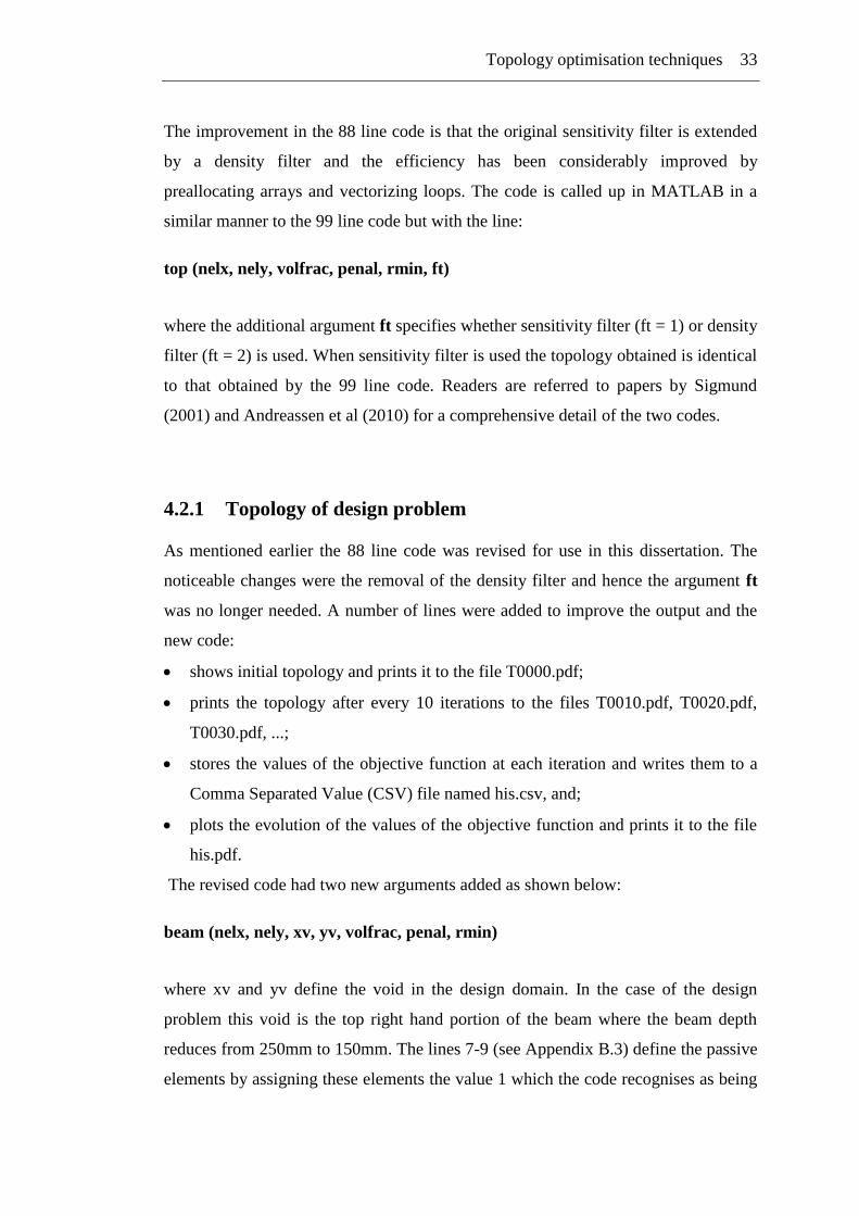
reinforce the beam accordingly to resist these forces. The theory behind this method
is that concrete in the compression side carries the compressive forces (Cc) as
illustrated in Figure 4.2. Steel reinforcement bars placed in the tensile zone resists the
tensile forces (T). If total compressive forces are greater than compressive strength of
concrete then steel reinforcement bars can be placed in the compression zone to resist
additional compressive forces (Cs). Readers can lookup Warner et al (2007) for
further information on reinforced concrete design basics.
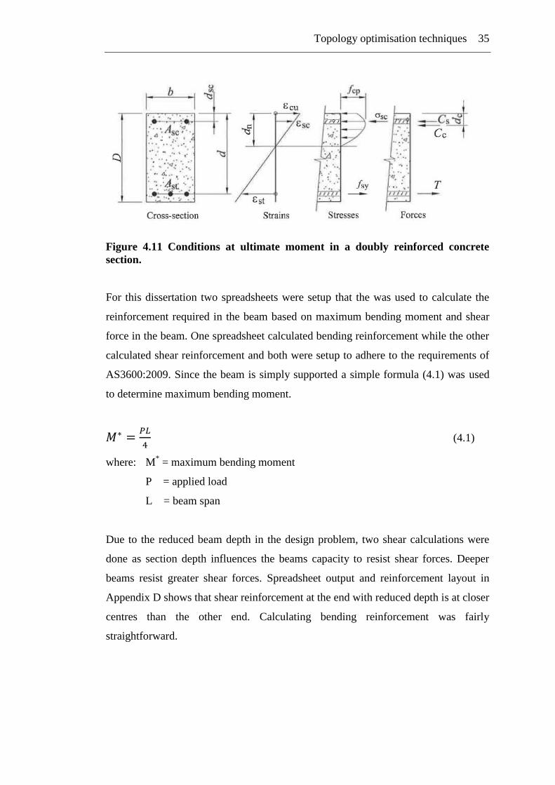
Topology optimisation techniques 35
Figure 4.11 Conditions at ultimate moment in a doubly reinforced concrete
section.
For this dissertation two spreadsheets were setup that the was used to calculate the
reinforcement required in the beam based on maximum bending moment and shear
force in the beam. One spreadsheet calculated bending reinforcement while the other
calculated shear reinforcement and both were setup to adhere to the requirements of
AS3600:2009. Since the beam is simply supported a simple formula (4.1) was used
to determine maximum bending moment.
(4.1)
where: M* = maximum bending moment
P = applied load
L = beam span
Due to the reduced beam depth in the design problem, two shear calculations were
done as section depth influences the beams capacity to resist shear forces. Deeper
beams resist greater shear forces. Spreadsheet output and reinforcement layout in
Appendix D shows that shear reinforcement at the end with reduced depth is at closer
centres than the other end. Calculating bending reinforcement was fairly
straightforward.
36 Topology optimisation techniques
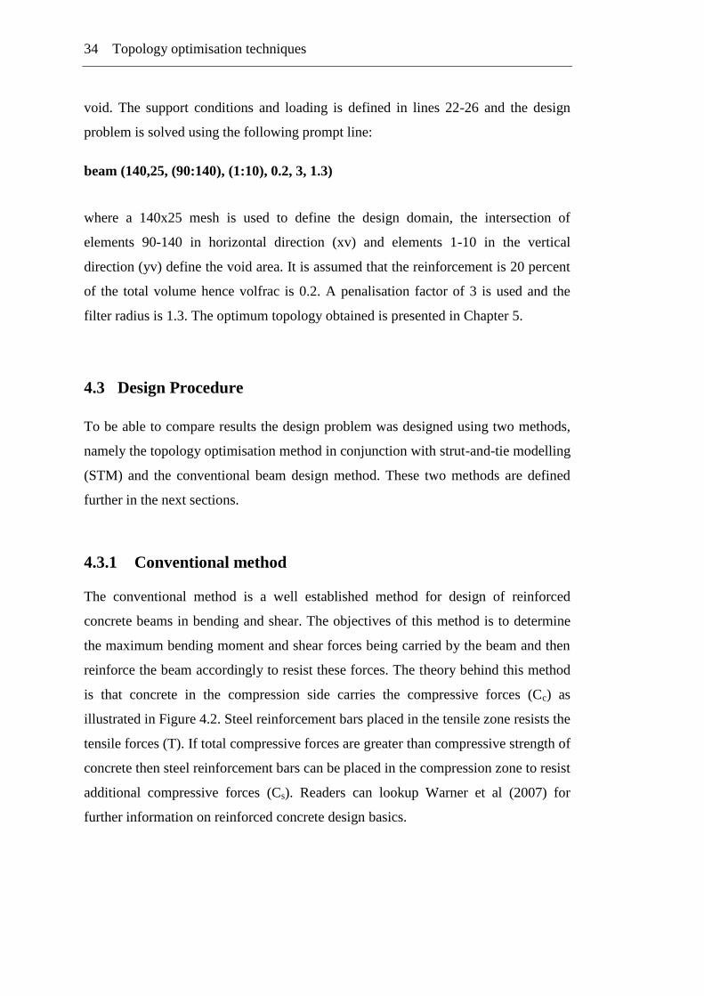
4.3.2 Strut-and-tie modelling method
The optimum topology that was obtained from the MATLAB code was modelled in
Microstran which is a finite element analysis software, to determine the internal
forces in the truss layout. Microstran outputs are presented in Appendix D.1. Once
the internal member forces were known the beam was designed using the provisions
of Section 7, AS3600:2009.
Provisions of AS3600:2009
Section 7 of this standard outlines the design of concrete structures using strut-and-
tie modelling method. The strut capacity C is:
(4.2)
where: Øst = is the strength reduction factor
βs = is the strut efficiency factor calculated by equation 4.3 below
fc’ = is the characteristic strength of concrete
Ac = is the cross section area of the strut.
The strut efficiency factor of prismatic strut (see figure 2.3a) is taken as 1.0 and for
fan or bottle-shaped strut is taken as;
(4.3)
where: θ = is the angle between the strut and tie axis
According to AS3600, prismatic struts should only be used where the compressive
stress cannot diverge, otherwise bottle-shaped strut should be used. The bursting
forces (figure 2.3c) in bottle-shaped struts need to be determined as given in section
7.4.2 of AS3600 and transverse reinforcement provided if needed.
The design strength of ties is similar to strength of tensile reinforcement in
conventional beam design. Hence;
Topology optimisation techniques 37
(4.4)
where: Ast = is the cross sectional area of reinforcement
fsy = is the yield strength of steel reinforcement
For unconfined nodal region the design strength shall be such that compressive stress
on any nodal face is not greater than , where:
for CCC node βn = 1.0;
for CCT node βn = 0.8;
for CTT node βn = 0.6.
Where confinement is provided the design strength shall not exceed maximum
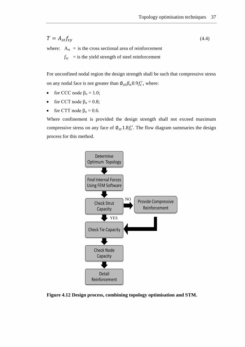
compressive stress on any face of . The flow diagram summaries the design
process for this method.
Figure 4.12 Design process, combining topology optimisation and STM.
NO
YES
38 Topology optimisation techniques
4.3.3 Concrete mix design
It was decided to use 40MPa concrete in the beam specimen and to achieve this the
following ratios were used.
Water/cement raito = 0.5
Aggregate/cement ratio = 3.5
Fine aggregate/course aggregate = 0.5
Based on the beam geometry it was calculated that about 0.035m3 of concrete would
be required and the water, cement and aggregate volumes were determined using the
above ratios. Sand and 10mm aggregate was used for fine aggregate while 15mm
aggregate was used as course aggregate. The concrete was mixed in a automated
mechanical mixer which ensured that the mix was consistent.
4.4 Finding Optimum Topology of Problems from Literature
To test the versatility of the topology optimisation code, the dissertation scope was
extended to determine optimum topology of standard problems found in literature.
These problems were mainly taken from papers on strut-and-tie modelling. This gave
a good opportunity to test if the optimum topology was comparable to the STM
layout the authors of those papers proposed.
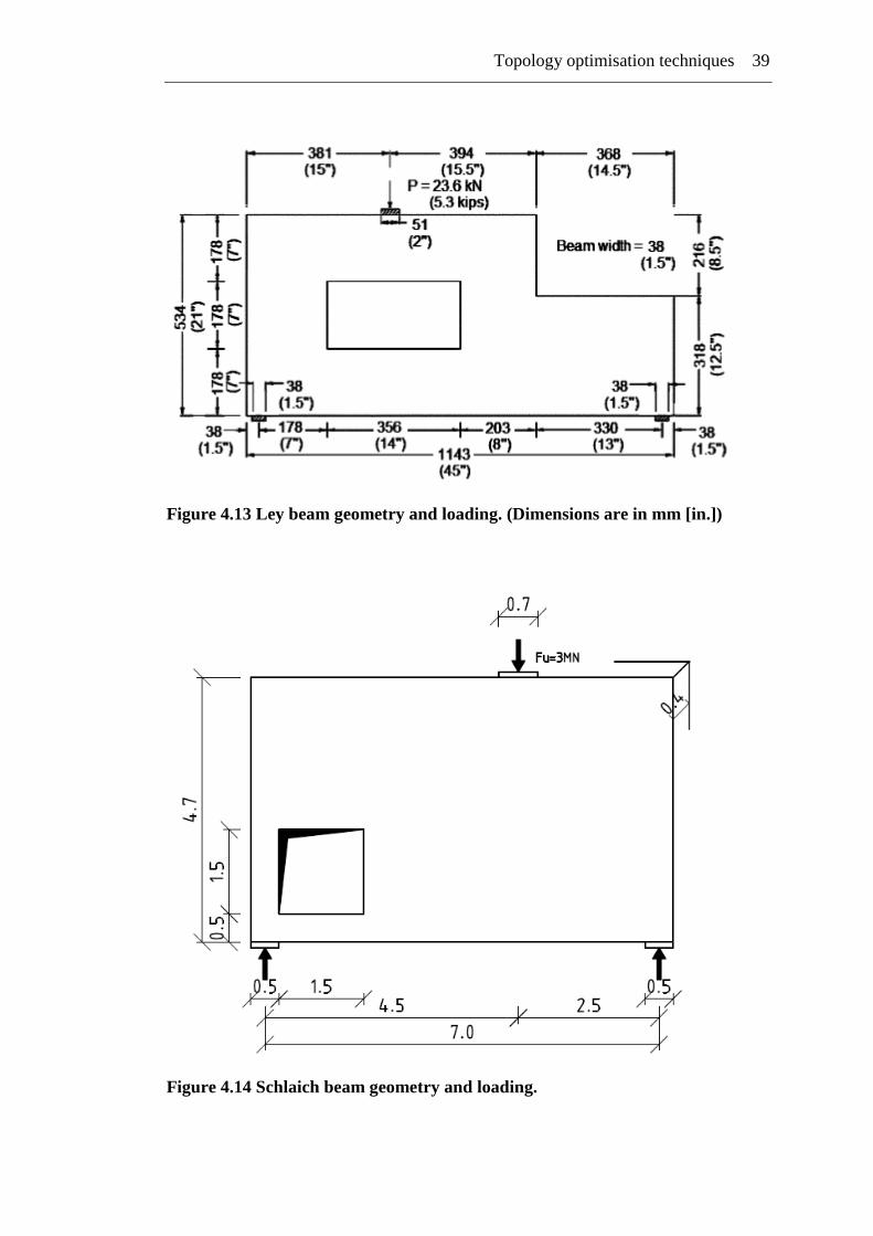
The first problem was the deep beam problem from the paper by Ley et al (2007). In
Figure 4.4 the beam is simply supported with a void in the middle and a point load is
acting above the void. In the paper by Ley et al (2007) 5 specimens are designed by
graduate students for different criteria such as using minimum steel, or limit
deflection. In the rest of the dissertation this beam will be referred as Ley beam.
Topology optimisation techniques 39
Figure 4.13 Ley beam geometry and loading. (Dimensions are in mm [in.])
Figure 4.14 Schlaich beam geometry and loading.
40 Topology optimisation techniques
The second problem was the deep beam presented by Schlaich et al (1987). It is
similar to Ley beam but it doesn‟t have any reduction in beam depth as can be seen
in Figure 4.5. The void is at the bottom left corner close to the support and a point
load is acting at about two thirds of the span.
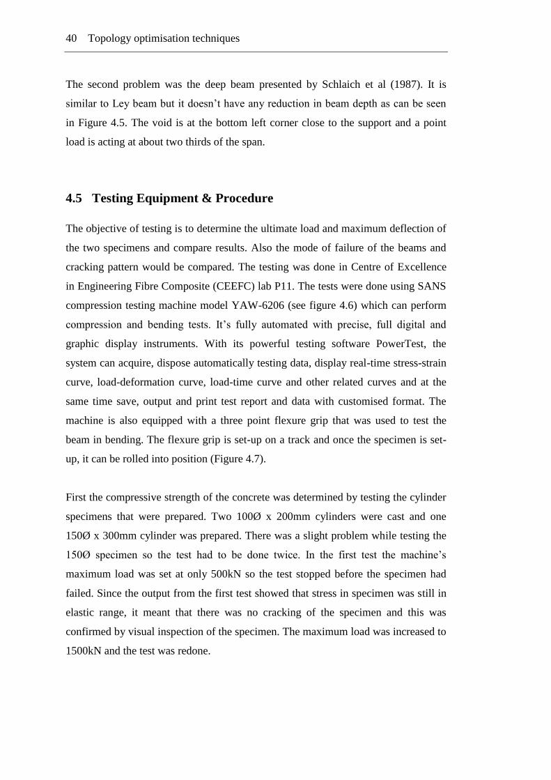
4.5 Testing Equipment & Procedure
The objective of testing is to determine the ultimate load and maximum deflection of
the two specimens and compare results. Also the mode of failure of the beams and
cracking pattern would be compared. The testing was done in Centre of Excellence
in Engineering Fibre Composite (CEEFC) lab P11. The tests were done using SANS
compression testing machine model YAW-6206 (see figure 4.6) which can perform
compression and bending tests. It‟s fully automated with precise, full digital and
graphic display instruments. With its powerful testing software PowerTest, the
system can acquire, dispose automatically testing data, display real-time stress-strain
curve, load-deformation curve, load-time curve and other related curves and at the
same time save, output and print test report and data with customised format. The
machine is also equipped with a three point flexure grip that was used to test the
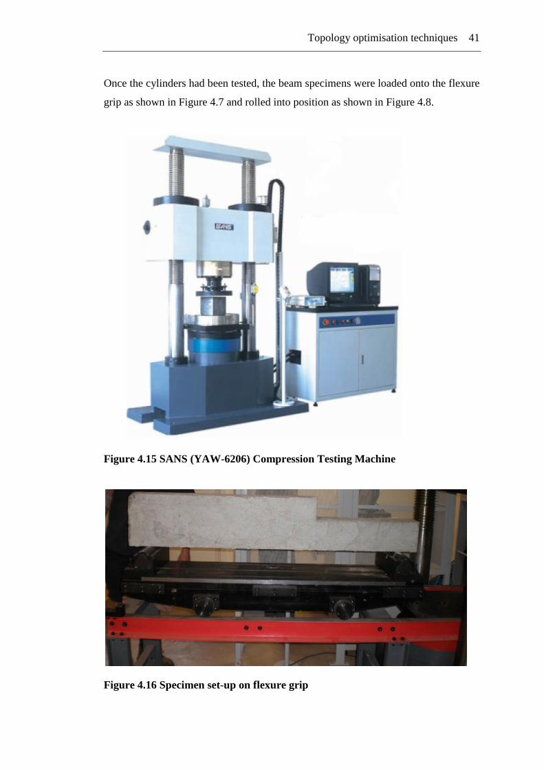
beam in bending. The flexure grip is set-up on a track and once the specimen is set-
up, it can be rolled into position (Figure 4.7).
First the compressive strength of the concrete was determined by testing the cylinder
specimens that were prepared. Two 100Ø x 200mm cylinders were cast and one
150Ø x 300mm cylinder was prepared. There was a slight problem while testing the
150Ø specimen so the test had to be done twice. In the first test the machine‟s
maximum load was set at only 500kN so the test stopped before the specimen had
failed. Since the output from the first test showed that stress in specimen was still in
elastic range, it meant that there was no cracking of the specimen and this was
confirmed by visual inspection of the specimen. The maximum load was increased to
1500kN and the test was redone.
Topology optimisation techniques 41
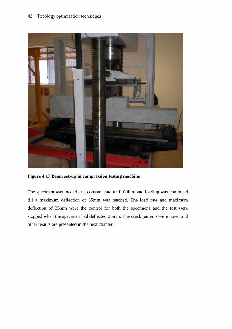
Once the cylinders had been tested, the beam specimens were loaded onto the flexure
grip as shown in Figure 4.7 and rolled into position as shown in Figure 4.8.
Figure 4.15 SANS (YAW-6206) Compression Testing Machine
Figure 4.16 Specimen set-up on flexure grip
42 Topology optimisation techniques
Figure 4.17 Beam set-up in compression testing machine
The specimen was loaded at a constant rate until failure and loading was continued
till a maximum deflection of 35mm was reached. The load rate and maximum
deflection of 35mm were the control for both the specimens and the test were
stopped when the specimen had deflected 35mm. The crack patterns were noted and
other results are presented in the next chapter.
Chapter 5
RESULTS
Overview
This chapter presents the results of the testing done and corresponding analysis and
interpretation of these results. Also provided here are the optimum topology
obtained for some of the beams found in literature and some discussion on its
similarity or differences to the original design.
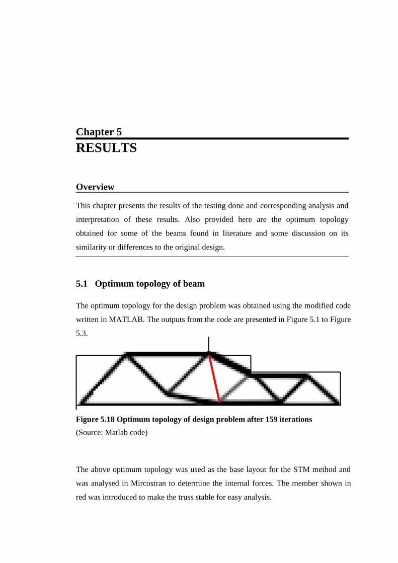
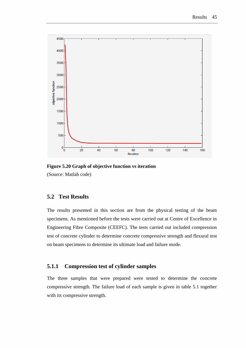
5.1 Optimum topology of beam
The optimum topology for the design problem was obtained using the modified code
written in MATLAB. The outputs from the code are presented in Figure 5.1 to Figure
5.3.
Figure 5.18 Optimum topology of design problem after 159 iterations
(Source: Matlab code)
The above optimum topology was used as the base layout for the STM method and
was analysed in Mircostran to determine the internal forces. The member shown in
red was introduced to make the truss stable for easy analysis.
44 Results
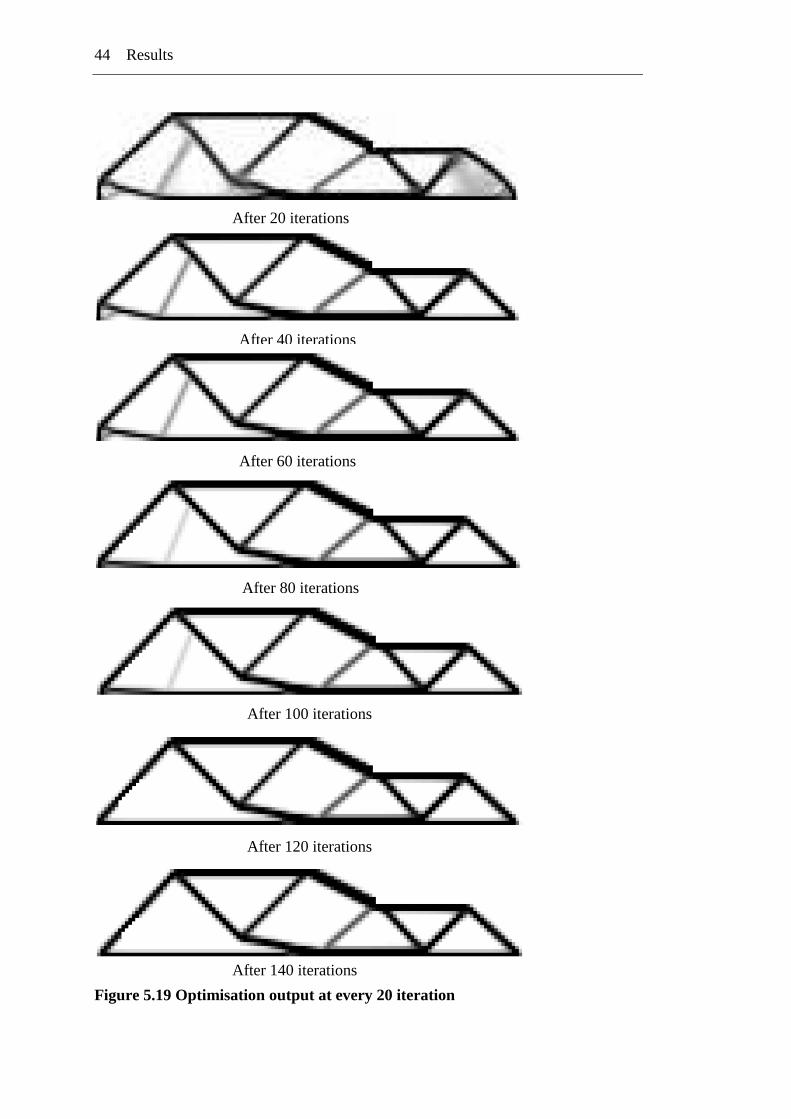
Figure 5.19 Optimisation output at every 20 iteration
After 20 iterations
After 40 iterations
After 60 iterations
After 80 iterations
After 100 iterations
After 120 iterations
After 140 iterations
Results 45
Figure 5.20 Graph of objective function vs iteration
(Source: Matlab code)
5.2 Test Results
The results presented in this section are from the physical testing of the beam
specimens. As mentioned before the tests were carried out at Centre of Excellence in
Engineering Fibre Composite (CEEFC). The tests carried out included compression
test of concrete cylinder to determine concrete compressive strength and flexural test
on beam specimens to determine its ultimate load and failure mode.
5.1.1 Compression test of cylinder samples
The three samples that were prepared were tested to determine the concrete
compressive strength. The failure load of each sample is given in table 5.1 together
with its compressive strength.
46 Results
Table 5.7 Cylinder test results
Specimen Dimension
(mm)
Failure load
(kN)
Compressive strength, fc‟
(MPa)
1 100Øx200 422.355 53.76
2 100Øx200 257.6 32.8
3 150Øx300 873.358 49.42
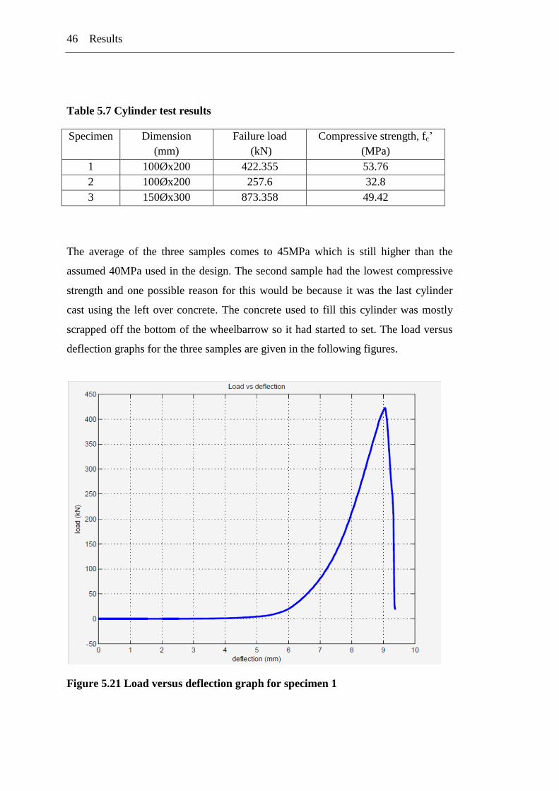
The average of the three samples comes to 45MPa which is still higher than the
assumed 40MPa used in the design. The second sample had the lowest compressive
strength and one possible reason for this would be because it was the last cylinder
cast using the left over concrete. The concrete used to fill this cylinder was mostly
scrapped off the bottom of the wheelbarrow so it had started to set. The load versus
deflection graphs for the three samples are given in the following figures.
Figure 5.21 Load versus deflection graph for specimen 1
Results 47
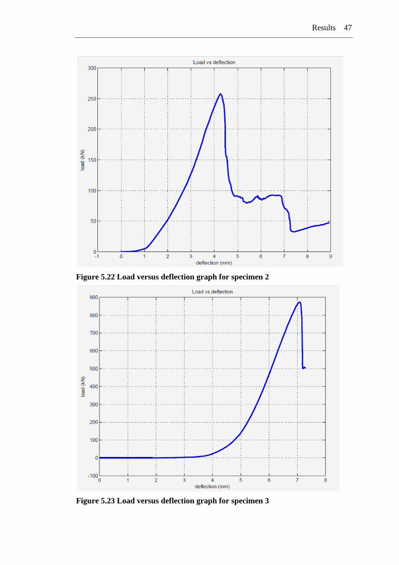
Figure 5.22 Load versus deflection graph for specimen 2
Figure 5.23 Load versus deflection graph for specimen 3
48 Results
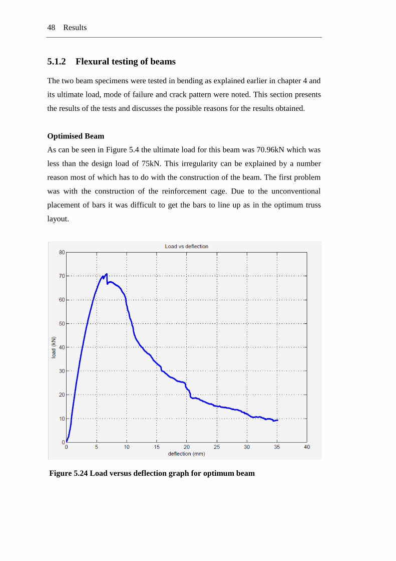
5.1.2 Flexural testing of beams
The two beam specimens were tested in bending as explained earlier in chapter 4 and
its ultimate load, mode of failure and crack pattern were noted. This section presents
the results of the tests and discusses the possible reasons for the results obtained.
Optimised Beam
As can be seen in Figure 5.4 the ultimate load for this beam was 70.96kN which was
less than the design load of 75kN. This irregularity can be explained by a number
reason most of which has to do with the construction of the beam. The first problem
was with the construction of the reinforcement cage. Due to the unconventional
placement of bars it was difficult to get the bars to line up as in the optimum truss
layout.
Figure 5.24 Load versus deflection graph for optimum beam
Results 49
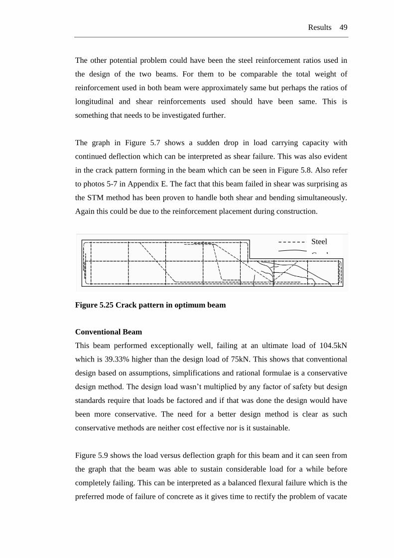
The other potential problem could have been the steel reinforcement ratios used in
the design of the two beams. For them to be comparable the total weight of
reinforcement used in both beam were approximately same but perhaps the ratios of
longitudinal and shear reinforcements used should have been same. This is
something that needs to be investigated further.
The graph in Figure 5.7 shows a sudden drop in load carrying capacity with
continued deflection which can be interpreted as shear failure. This was also evident
in the crack pattern forming in the beam which can be seen in Figure 5.8. Also refer
to photos 5-7 in Appendix E. The fact that this beam failed in shear was surprising as
the STM method has been proven to handle both shear and bending simultaneously.
Again this could be due to the reinforcement placement during construction.
Figure 5.25 Crack pattern in optimum beam
Conventional Beam
This beam performed exceptionally well, failing at an ultimate load of 104.5kN
which is 39.33% higher than the design load of 75kN. This shows that conventional
design based on assumptions, simplifications and rational formulae is a conservative
design method. The design load wasn‟t multiplied by any factor of safety but design
standards require that loads be factored and if that was done the design would have
been more conservative. The need for a better design method is clear as such
conservative methods are neither cost effective nor is it sustainable.
Figure 5.9 shows the load versus deflection graph for this beam and it can seen from
the graph that the beam was able to sustain considerable load for a while before
completely failing. This can be interpreted as a balanced flexural failure which is the
preferred mode of failure of concrete as it gives time to rectify the problem of vacate
Steel
Cracks
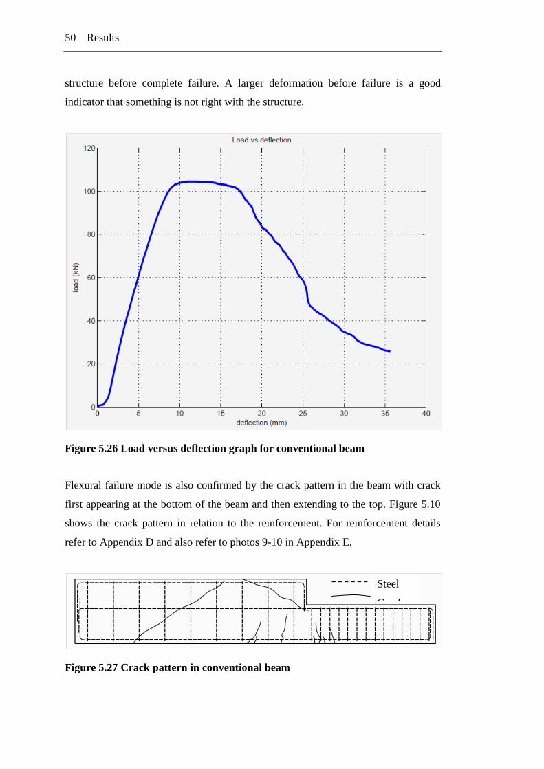
50 Results
structure before complete failure. A larger deformation before failure is a good
indicator that something is not right with the structure.
Figure 5.26 Load versus deflection graph for conventional beam
Flexural failure mode is also confirmed by the crack pattern in the beam with crack
first appearing at the bottom of the beam and then extending to the top. Figure 5.10
shows the crack pattern in relation to the reinforcement. For reinforcement details
refer to Appendix D and also refer to photos 9-10 in Appendix E.
Figure 5.27 Crack pattern in conventional beam
Steel
Cracks
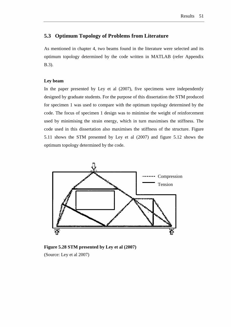
Results 51
5.3 Optimum Topology of Problems from Literature
As mentioned in chapter 4, two beams found in the literature were selected and its
optimum topology determined by the code written in MATLAB (refer Appendix
B.3).
Ley beam
In the paper presented by Ley et al (2007), five specimens were independently
designed by graduate students. For the purpose of this dissertation the STM produced
for specimen 1 was used to compare with the optimum topology determined by the
code. The focus of specimen 1 design was to minimise the weight of reinforcement
used by minimising the strain energy, which in turn maximises the stiffness. The
code used in this dissertation also maximises the stiffness of the structure. Figure
5.11 shows the STM presented by Ley et al (2007) and figure 5.12 shows the
optimum topology determined by the code.
Figure 5.28 STM presented by Ley et al (2007)
(Source: Ley et al 2007)
Compression
Tension
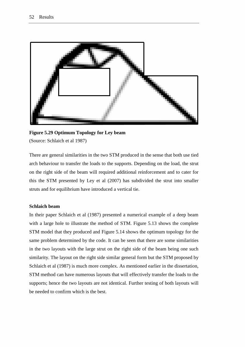
52 Results
Figure 5.29 Optimum Topology for Ley beam
(Source: Schlaich et al 1987)
There are general similarities in the two STM produced in the sense that both use tied
arch behaviour to transfer the loads to the supports. Depending on the load, the strut
on the right side of the beam will required additional reinforcement and to cater for
this the STM presented by Ley et al (2007) has subdivided the strut into smaller
struts and for equilibrium have introduced a vertical tie.
Schlaich beam
In their paper Schlaich et al (1987) presented a numerical example of a deep beam
with a large hole to illustrate the method of STM. Figure 5.13 shows the complete
STM model that they produced and Figure 5.14 shows the optimum topology for the
same problem determined by the code. It can be seen that there are some similarities
in the two layouts with the large strut on the right side of the beam being one such
similarity. The layout on the right side similar general form but the STM proposed by
Schlaich et al (1987) is much more complex. As mentioned earlier in the dissertation,
STM method can have numerous layouts that will effectively transfer the loads to the
supports; hence the two layouts are not identical. Further testing of both layouts will
be needed to confirm which is the best.
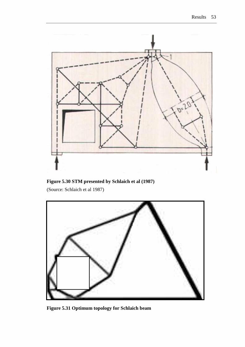
Results 53
Figure 5.30 STM presented by Schlaich et al (1987)
(Source: Schlaich et al 1987)
Figure 5.31 Optimum topology for Schlaich beam

This page has been left intentionally blank
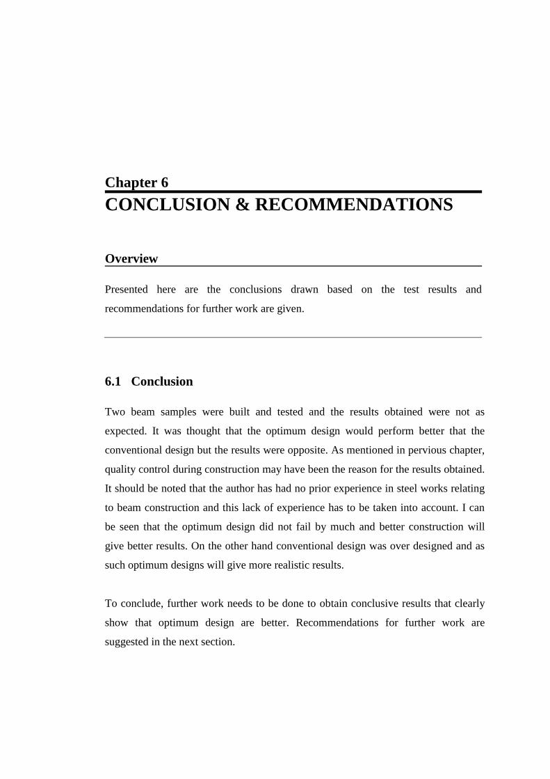
Chapter 6
CONCLUSION & RECOMMENDATIONS
Overview
Presented here are the conclusions drawn based on the test results and
recommendations for further work are given.
6.1 Conclusion
Two beam samples were built and tested and the results obtained were not as
expected. It was thought that the optimum design would perform better that the
conventional design but the results were opposite. As mentioned in pervious chapter,
quality control during construction may have been the reason for the results obtained.
It should be noted that the author has had no prior experience in steel works relating
to beam construction and this lack of experience has to be taken into account. I can
be seen that the optimum design did not fail by much and better construction will
give better results. On the other hand conventional design was over designed and as
such optimum designs will give more realistic results.
To conclude, further work needs to be done to obtain conclusive results that clearly
show that optimum design are better. Recommendations for further work are
suggested in the next section.

56 Conclusion and recommendations
6.2 Recommendations for Future Work
The optimum beam may need to be redesigned, built and testing to get conclusive
results. Due to time constraints this was not done for this dissertation but this may be
done by the author at a later stage as part of his further research in this topic.
As mentioned better construction techniques need to be used so that reinforcement
can be easily placed in the steel cage. It‟s was also noted that the ratios for the total
steel reinforcement in the two beams were same but for a better comparison the
ratios of longitudinal and shear reinforcements need to be similar.
It may also be of great advantage to use strain gauges to determine deflections at
various locations along the beam to analyse the beam behaviour under load.
Bibliography
Andreassen, E., Clausen, A., Schevenels, M., Lazarov, B., and Sigmund, O. (2011).
Efficient topology optimization in MATLAB using 88 lines of code. structural
and multidisciplinary optimization, Vol. 43, No 1, pp. 1-16.
Burns, S.A. (Ed), (2002) Recent Advances in Optimal Structural Design. Virginia:
American Society of Civil Engineers.
Burns, T. E. (2005) A reevaluation of the SIMP method with filtering and an
alternative formulation for solid-void topology optimization, Structural and
Multidisciplinary Optimization, Vol. 30, No. 6, pp. 428-436.
Bendsoe, M. P. (1989) Optimal shape design as a material distribution problem.
Structural and Multidisciplinary Optimization, Vol. 1, No. 4, pp. 193-202.
Bendsoe, M. P. and Kikuchi, N. (1988) Generating optimal topologies in structural
design using a homogenization method. Computer Methods in Applied Mechanics
and Engineering, Vol. 71, No. 2, pp. 197-224.
Bendsoe, M. P. and Sigmund, O. (1999) Material interpolation schemes in topology
optimization. Archive of Applied Mechanics, Vol. 69. Nos. 9-10, pp. 635-654.
Bendsoe, M. P. and Sigmund, O. (2003) Topology Optimization – Theory, Methods
and Applications. Berlin: Springer-Verlag.
Cheng, K.-T. and Olhoff, N. (1981) An investigation concerning optimal design of
solid elastic plates. International Journal of Solids and Structures, Vol. 17, No. 3,
pp. 305-323.
58 Bibliography
Eschenauer, H. A. and Olhoff, N, (2001) Topology optimization of continuum
structures: A review. Applied Mechanics Reviews, Vol. 54, No. 4, pp. 331-390.
Ghabrie, K. (2010) Optimising the reinforcement design of reinforced concrete
members using topology optimisation techniques.
Guan, H. (2004) Strut-and-tie model of deep beams with web openings – an
optimization approach. Structural and Engineering Mechanics, Vol. 19, No. 4, pp.
361-379.
Hassani, B., Hinton, E. (1998a) A review of homogenization and topology
optimization I – homogenization theory for media with periodic structure,
Computers & Structures, Vol. 69, No. 6, pp. 707-717.
Hassani, B. and Hinton, E. (1998b) A review of homogenization and topology
optimization II – analytical and numerical solution of homogenization equations,
Computers & Structures, Vol. 69, No. 6, pp. 718-738.
Hassani, B. and Hinton, E. (1998c) A review of homogenization and topology
optimization III – topology optimization using optimality criteria, Computers &
Structures, Vol. 69, No. 6, pp. 707-717.
Huang, X. and Xie, Y. M. (2010) Evolutionary Topology Optimization of Continuum
Structures – Methods and Applications. West Sussex (UK): Wiley.
Kohn, R. V. and Strang, G. (1986) Optimal design and relaxation of variational
problems, Communications on Pure and Applied Mathematics, Vol. 39, Part I
113-137; Part II 139-182; Part III 353-377.
Ley, M. T., Riding, K. A., Widianto, Sungjin, B. and Breen, J. E. (2007)
Experimental verification of strut and tie model design method. ACI Structural
Journal, Vol. 104, No. 6, pp. 749-755.
Bibliography 59
Liang, Q. Q., Uy, B. and Steven, P. G. (2002) Performance-based optimization for
strut-tie modeling of structural concrete. Journal of Structural Engineering, Vol.
128, No. 6, pp. 815-824.
Liang, Q. Q. (2005) Performance-based Optimization of Structures – Theory and
applications. Oxon: Spon Press.
Ma, D. Z., Wang, H., Kikuchi, N., Pierre, C. and Raju, B. (2006) Experimental
validation and prototyping of optimum designs obtained from topology
optimization. Structural Multidisciplinary Optimization, Vol. 31, No. 5, pp. 333-
343.
Maxwell, J. C. (1890) On reciprocal figures, frames and diagrams of forces,
Scientific Papers, Cambridge University Press, 2, pp. 175-177.
Marti, P. (1985) Basic Tools of Reinforced Concrete Design, ACI Journal, Vol. 82,
No. 1, pp. 46-56.
Michell, A.G.M. (1904) The limits of economy of frame structures, Philosophical
Magazine, sect. 6, 8: 589-597.
Nagarajan, P. and Pillai, T. M. M. (2008) Analysis and deisgn of simply supported
deep beams using strut and tie method. Advances in Structural Engineering, Vol.
11, No. 5, pp. 491-499.
Nilson, A. H., Darwin, D. And Dolan, C. H. (2004) Design of Concrete Structures.
New York: McGraw Hill.
Park, J.-W. and Kuchma, D. (2007) Strut-and-tie model analysis for strength
prediction of deep beams. ACI Structural Journal, Vol. 104, No. 6, pp. 657-666.
60 Bibliography
Prager, W. (1969) Optimality cretria derived from classical extermum principles.
Technical report, SM Studies Series, Solid Mechanics Division, University of
Waterloo, Ontario, Canada.
Prager, W. (1974) A note on discretized michell structures. Computer Methods in
Applied Mechanics and Engineering, Vol. 3. No. 3, pp. 349-355.
Querin, O. M., Steven, G. P. and Xie, Y. M. (1998) Evolutionary structural
optimization (eso) using a bidirectional algorithm. Engineering Computations,
Vol. 15. No. 8, pp. 1031-1048.
Quintero-Febres, C. G., Parra-Montesonis, G. and Wight, J. K (2006) Strength of
Struts in Deep Concrete Members Designed Using Strut-and-Tie Method. ACI
Structural Journal, Vol. 103, No. 4, pp. 577-586.
Rozvanny, G.I.N. (1972a) Grillages of maximum strength and maximum stiffness.
International Journal of Mechanical Sciences, Vol. 14. No.10, pp. 651-666.
Rozvanny, G.I.N. (1972b) Optimal load transmission by flexure. Computer Method
in Applied Mechanics and Engineering, Vol. 1, No. 3, pp. 253-263.
Rozvanny, G.I.N. (2001) Aims, scope, methods, history and unified terminology of
computer-aided topology optimization in structural mechanics. Structural and
Multidisciplinary Optimization, Vol. 21, No. 2, pp. 90-108.
Rozvanny, G.I.N. (2009) A critical review of established methods of structural
topology optimization. Structural Multidisciplinary Optimization, Vol. 37, No. 3,
pp. 217-237.
Rozvanny, G.I.N. and Prager, W. (1976) Optimal design of partially discretized
grillages. Journal of the Mechanics and Physics of Solids, Vol. 24, No. 2-3, pp.
125-136.
Bibliography 61
Schlaich, J., Schafer, K. and Jennewein, M. (1987) Toward a consistent design of
structural concrete. PCI Journal, Vol. 32, No. 3, pp. 74-150.
Schlaich, J. and Schafer, K (1991) Design and detailing of structural concrete using
strut-and-tie models. Structural Engineer, Vol. 69, No. 6, pp. 113-125.
Sigmund, O. (2001) A 99 line topology optimization code written in Matlab,
Strcutural Multidisciplinary Optimization, Vol. 21, No. 2, pp. 120-127.
Sigumnd, O. and Petersson, J. (1998) Instabilities in topology optimization - A
survey on procedures dealing with checkerboard, mesh-dependencies and local
minima. Structural and Multidisciplinary Optimization, Vol. 16, No, 1, pp. 68-75.
Warner, R.F., Foster, S.J., and Kilpatrick, A.E. (2007) Reinforced Concrete Basics,
2nd Edition, Frenchs Forest, NSW: Pearson Prentice Hall.
Wang, M. Y., Wang, X. and Guo, D. (2003) A level set method for structural
topology optimization. Computer Methods in Applied Mechanics and
Engineering, Vol. 192, Nos. 1-2, pp. 227-246.
Wight, J. K. and Parra-Montesonis, G. J. Strut-and-tie model for deep beams.
Concrete International, May, 2003, pp. 63-70.
Xie, Y. M. and Steven, G. P. (1993) A simple evolutionary procedure for structural
optimisation. Computers and Structures, Vol. 49, No. 5, pp. 885-896.
Yun, Y. M. and Ramirez, J. A. (1996) Strength of Struts and Nodes in Strut-Tie
Model. ASCE Journal of Structural Engineering, Vol. 122, No. 1, pp. 20-30.

62 Bibliography
Zuo, K. T., Chen, P. L., Zhang, Q. Y. and Yang, J. (2007) Study of key algorithms in
topology optimization, The International Journal of Advanced Manufacturing
Technology, Vol. 32, Nos. 7-8, pp. 787-796.

Appendix A – Specification
University of Southern Queensland
FACULTY OF ENGINEERING AND SURVEYING
ENG4111/4112 Research Project
PROJECT SPECIFICATION
FOR: Nitesh Nitin PRASAD
TOPIC: VERIFICATION OF SIMPLIFIED OPTIMUM DESIGNS FOR
REINFORCED CONCRETE DEEP BEAMS
SUPERVISOR: Dr Kazem Ghabraie
PROJECT AIM: To verify optimum designs obtained by using a simplified linear
elastic model for reinforced concrete.
PROGRAMME:
1. Research background information relating to topology optimisation, especially
the SIMP method.
2. Research on concrete beam design by strut-and-tie method.
3. Design the given deep beam using strut-and-tie method.
4. Optimise design obtained in (3) using the Matlab optimisation
code.
5. Prepare samples based on strut-and-tie design and optimised
design.
6. Test samples and compare results.
7. Conclusions.
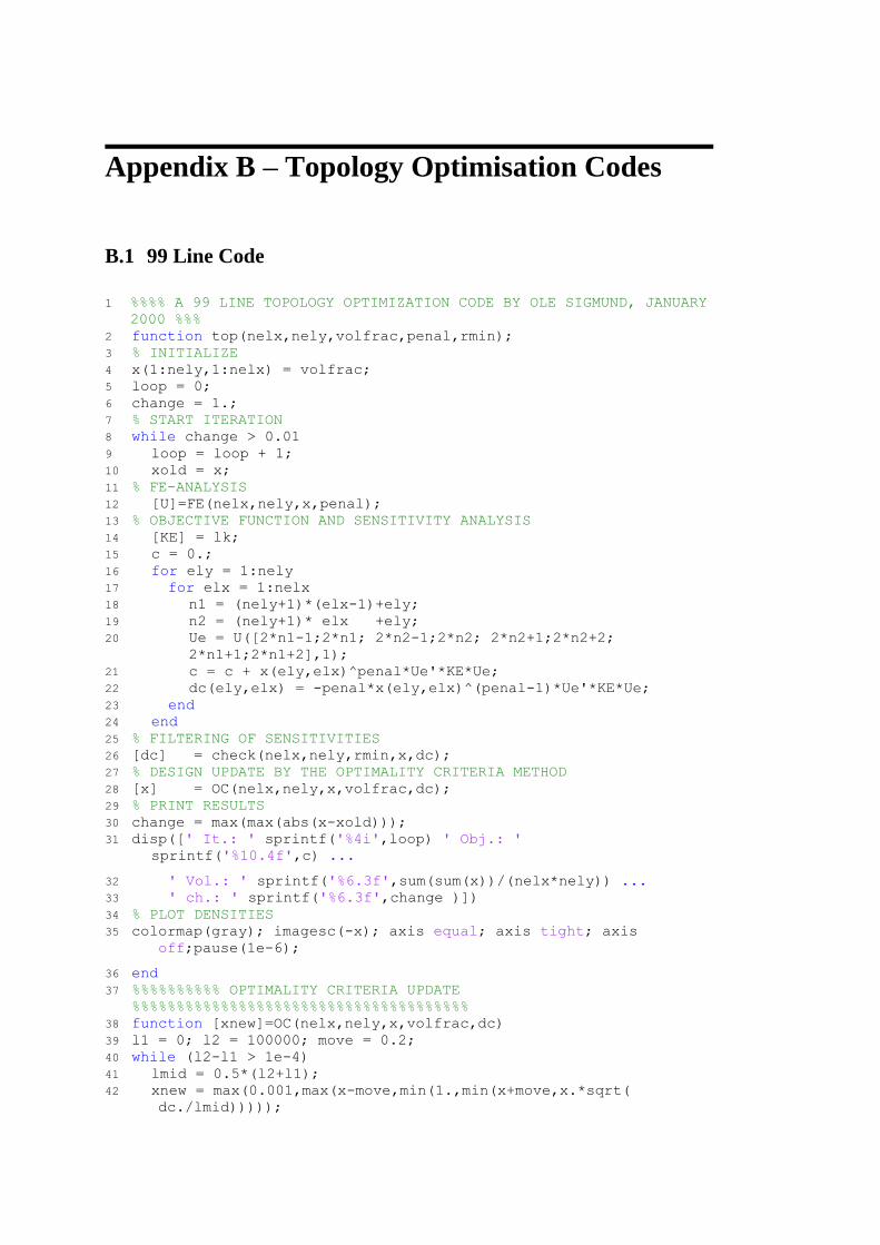
Appendix B – Topology Optimisation Codes
B.1 99 Line Code
1 %%%% A 99 LINE TOPOLOGY OPTIMIZATION CODE BY OLE SIGMUND, JANUARY
2000 %%% 2 function top(nelx,nely,volfrac,penal,rmin); 3 % INITIALIZE 4 x(1:nely,1:nelx) = volfrac; 5 loop = 0; 6 change = 1.; 7 % START ITERATION 8 while change > 0.01 9 loop = loop + 1; 10 xold = x; 11 % FE-ANALYSIS 12 [U]=FE(nelx,nely,x,penal); 13 % OBJECTIVE FUNCTION AND SENSITIVITY ANALYSIS 14 [KE] = lk; 15 c = 0.; 16 for ely = 1:nely 17 for elx = 1:nelx 18 n1 = (nely+1)*(elx-1)+ely; 19 n2 = (nely+1)* elx +ely; 20 Ue = U([2*n1-1;2*n1; 2*n2-1;2*n2; 2*n2+1;2*n2+2;
2*n1+1;2*n1+2],1); 21 c = c + x(ely,elx)^penal*Ue'*KE*Ue; 22 dc(ely,elx) = -penal*x(ely,elx)^(penal-1)*Ue'*KE*Ue; 23 end 24 end 25 % FILTERING OF SENSITIVITIES 26 [dc] = check(nelx,nely,rmin,x,dc); 27 % DESIGN UPDATE BY THE OPTIMALITY CRITERIA METHOD 28 [x] = OC(nelx,nely,x,volfrac,dc); 29 % PRINT RESULTS 30 change = max(max(abs(x-xold))); 31 disp([' It.: ' sprintf('%4i',loop) ' Obj.: '
sprintf('%10.4f',c) ...
32 ' Vol.: ' sprintf('%6.3f',sum(sum(x))/(nelx*nely)) ... 33 ' ch.: ' sprintf('%6.3f',change )]) 34 % PLOT DENSITIES 35 colormap(gray); imagesc(-x); axis equal; axis tight; axis
off;pause(1e-6);
36 end 37 %%%%%%%%%% OPTIMALITY CRITERIA UPDATE
%%%%%%%%%%%%%%%%%%%%%%%%%%%%%%%%%%%%%% 38 function [xnew]=OC(nelx,nely,x,volfrac,dc) 39 l1 = 0; l2 = 100000; move = 0.2; 40 while (l2-l1 > 1e-4) 41 lmid = 0.5*(l2+l1); 42 xnew = max(0.001,max(x-move,min(1.,min(x+move,x.*sqrt(
dc./lmid)))));
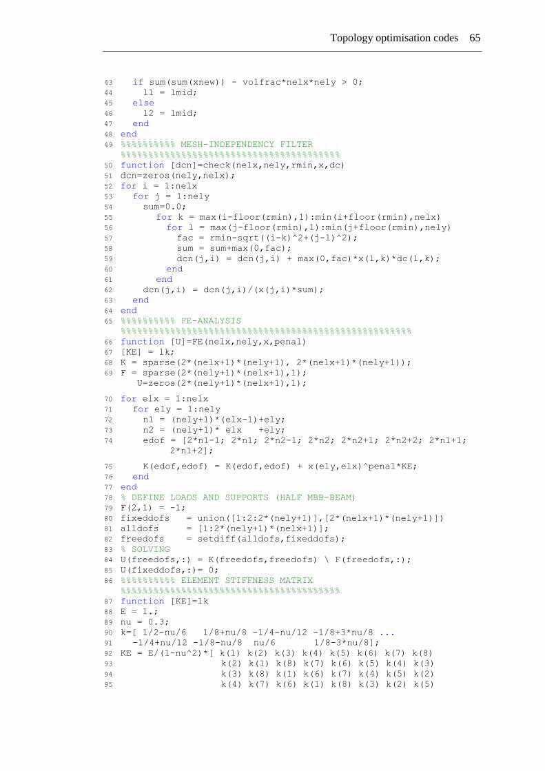
Topology optimisation codes 65
43 if sum(sum(xnew)) - volfrac*nelx*nely > 0; 44 l1 = lmid; 45 else 46 l2 = lmid; 47 end 48 end 49 %%%%%%%%%% MESH-INDEPENDENCY FILTER
%%%%%%%%%%%%%%%%%%%%%%%%%%%%%%%%%%%%%%%% 50 function [dcn]=check(nelx,nely,rmin,x,dc) 51 dcn=zeros(nely,nelx); 52 for i = 1:nelx 53 for j = 1:nely 54 sum=0.0; 55 for k = max(i-floor(rmin),1):min(i+floor(rmin),nelx) 56 for l = max(j-floor(rmin),1):min(j+floor(rmin),nely) 57 fac = rmin-sqrt((i-k)^2+(j-l)^2); 58 sum = sum+max(0,fac); 59 dcn(j,i) = dcn(j,i) + max(0,fac)*x(l,k)*dc(l,k); 60 end 61 end 62 dcn(j,i) = dcn(j,i)/(x(j,i)*sum); 63 end 64 end 65 %%%%%%%%%% FE-ANALYSIS
%%%%%%%%%%%%%%%%%%%%%%%%%%%%%%%%%%%%%%%%%%%%%%%%%%%%% 66 function [U]=FE(nelx,nely,x,penal) 67 [KE] = lk; 68 K = sparse(2*(nelx+1)*(nely+1), 2*(nelx+1)*(nely+1)); 69 F = sparse(2*(nely+1)*(nelx+1),1);
U=zeros(2*(nely+1)*(nelx+1),1);
70 for elx = 1:nelx 71 for ely = 1:nely 72 n1 = (nely+1)*(elx-1)+ely; 73 n2 = (nely+1)* elx +ely; 74 edof = [2*n1-1; 2*n1; 2*n2-1; 2*n2; 2*n2+1; 2*n2+2; 2*n1+1;
2*n1+2];
75 K(edof,edof) = K(edof,edof) + x(ely,elx)^penal*KE; 76 end 77 end 78 % DEFINE LOADS AND SUPPORTS (HALF MBB-BEAM) 79 F(2,1) = -1; 80 fixeddofs = union([1:2:2*(nely+1)],[2*(nelx+1)*(nely+1)]) 81 alldofs = [1:2*(nely+1)*(nelx+1)]; 82 freedofs = setdiff(alldofs,fixeddofs); 83 % SOLVING 84 U(freedofs,:) = K(freedofs,freedofs) \ F(freedofs,:); 85 U(fixeddofs,:)= 0; 86 %%%%%%%%%% ELEMENT STIFFNESS MATRIX
%%%%%%%%%%%%%%%%%%%%%%%%%%%%%%%%%%%%%%%% 87 function [KE]=lk 88 E = 1.; 89 nu = 0.3; 90 k=[ 1/2-nu/6 1/8+nu/8 -1/4-nu/12 -1/8+3*nu/8 ... 91 -1/4+nu/12 -1/8-nu/8 nu/6 1/8-3*nu/8]; 92 KE = E/(1-nu^2)*[ k(1) k(2) k(3) k(4) k(5) k(6) k(7) k(8) 93 k(2) k(1) k(8) k(7) k(6) k(5) k(4) k(3) 94 k(3) k(8) k(1) k(6) k(7) k(4) k(5) k(2) 95 k(4) k(7) k(6) k(1) k(8) k(3) k(2) k(5)
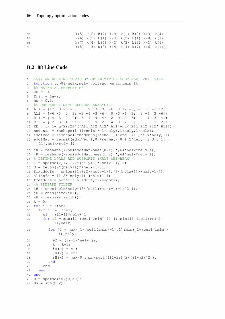
66 Topology optimisation codes
96 k(5) k(6) k(7) k(8) k(1) k(2) k(3) k(4) 97 k(6) k(5) k(4) k(3) k(2) k(1) k(8) k(7) 98 k(7) k(4) k(5) k(2) k(3) k(8) k(1) k(6) 99 k(8) k(3) k(2) k(5) k(4) k(7) k(6) k(1)];
B.2 88 Line Code
1 %%%% AN 88 LINE TOPOLOGY OPTIMIZATION CODE Nov, 2010 %%%% 2 function top88(nelx,nely,volfrac,penal,rmin,ft) 3 %% MATERIAL PROPERTIES 4 E0 = 1; 5 Emin = 1e-9; 6 nu = 0.3; 7 %% PREPARE FINITE ELEMENT ANALYSIS 8 A11 = [12 3 -6 -3; 3 12 3 0; -6 3 12 -3; -3 0 -3 12]; 9 A12 = [-6 -3 0 3; -3 -6 -3 -6; 0 -3 -6 3; 3 -6 3 -6]; 10 B11 = [-4 3 -2 9; 3 -4 -9 4; -2 -9 -4 -3; 9 4 -3 -4]; 11 B12 = [ 2 -3 4 -9; -3 2 9 -2; 4 9 2 3; -9 -2 3 2]; 12 KE = 1/(1-nu^2)/24*([A11 A12;A12' A11]+nu*[B11 B12;B12' B11]); 13 nodenrs = reshape(1:(1+nelx)*(1+nely),1+nely,1+nelx); 14 edofVec = reshape(2*nodenrs(1:end-1,1:end-1)+1,nelx*nely,1); 15 edofMat = repmat(edofVec,1,8)+repmat([0 1 2*nely+[2 3 0 1] –
21],nelx*nely,1);
16 iK = reshape(kron(edofMat,ones(8,1))',64*nelx*nely,1); 17 jK = reshape(kron(edofMat,ones(1,8))',64*nelx*nely,1); 18 % DEFINE LOADS AND SUPPORTS (HALF MBB-BEAM) 19 F = sparse(2,1,-1,2*(nely+1)*(nelx+1),1); 20 U = zeros(2*(nely+1)*(nelx+1),1); 21 fixeddofs = union([1:2:2*(nely+1)],[2*(nelx+1)*(nely+1)]); 22 alldofs = [1:2*(nely+1)*(nelx+1)]; 23 freedofs = setdiff(alldofs,fixeddofs); 24 %% PREPARE FILTER 25 iH = ones(nelx*nely*(2*(ceil(rmin)-1)+1)^2,1); 26 jH = ones(size(iH)); 27 sH = zeros(size(iH)); 28 k = 0; 29 for i1 = 1:nelx 30 for j1 = 1:nely 31 e1 = (i1-1)*nely+j1; 32 for i2 = max(i1-(ceil(rmin)-1),1):min(i1+(ceil(rmin)-
1),nelx)
33 for j2 = max(j1-(ceil(rmin)-1),1):min(j1+(ceil(rmin)- 1),nely)
34 e2 = (i2-1)*nely+j2; 35 k = k+1; 36 iH(k) = e1; 37 jH(k) = e2; 38 sH(k) = max(0,rmin-sqrt((i1-i2)^2+(j1-j2)^2)); 39 end 40 end 41 end 42 end 43 H = sparse(iH,jH,sH); 44 Hs = sum(H,2);
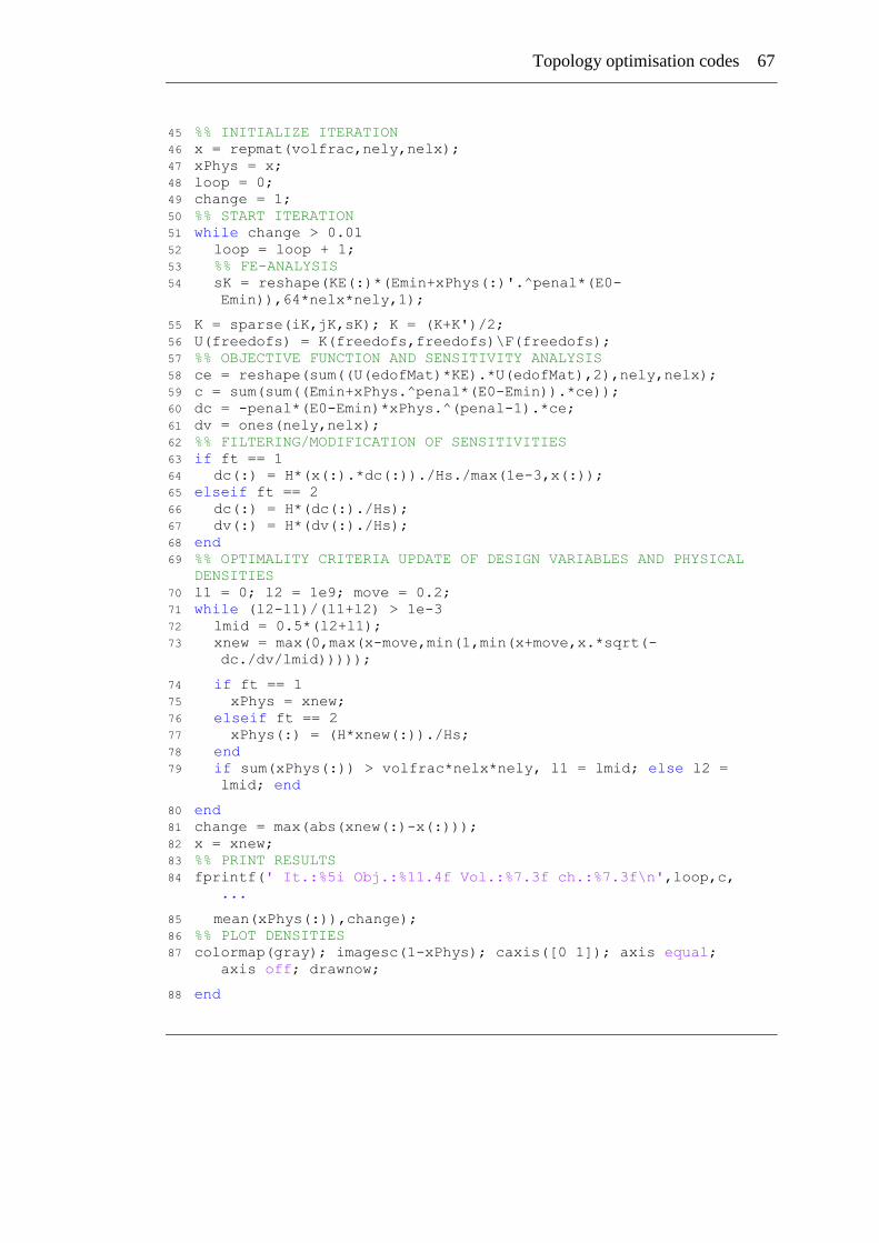
Topology optimisation codes 67
45 %% INITIALIZE ITERATION 46 x = repmat(volfrac,nely,nelx); 47 xPhys = x; 48 loop = 0; 49 change = 1; 50 %% START ITERATION 51 while change > 0.01 52 loop = loop + 1; 53 %% FE-ANALYSIS 54 sK = reshape(KE(:)*(Emin+xPhys(:)'.^penal*(E0-
Emin)),64*nelx*nely,1);
55 K = sparse(iK,jK,sK); K = (K+K')/2; 56 U(freedofs) = K(freedofs,freedofs)\F(freedofs); 57 %% OBJECTIVE FUNCTION AND SENSITIVITY ANALYSIS 58 ce = reshape(sum((U(edofMat)*KE).*U(edofMat),2),nely,nelx); 59 c = sum(sum((Emin+xPhys.^penal*(E0-Emin)).*ce)); 60 dc = -penal*(E0-Emin)*xPhys.^(penal-1).*ce; 61 dv = ones(nely,nelx); 62 %% FILTERING/MODIFICATION OF SENSITIVITIES 63 if ft == 1 64 dc(:) = H*(x(:).*dc(:))./Hs./max(1e-3,x(:)); 65 elseif ft == 2 66 dc(:) = H*(dc(:)./Hs); 67 dv(:) = H*(dv(:)./Hs); 68 end 69 %% OPTIMALITY CRITERIA UPDATE OF DESIGN VARIABLES AND PHYSICAL
DENSITIES 70 l1 = 0; l2 = 1e9; move = 0.2; 71 while (l2-l1)/(l1+l2) > 1e-3 72 lmid = 0.5*(l2+l1); 73 xnew = max(0,max(x-move,min(1,min(x+move,x.*sqrt(-
dc./dv/lmid)))));
74 if ft == 1 75 xPhys = xnew; 76 elseif ft == 2 77 xPhys(:) = (H*xnew(:))./Hs; 78 end 79 if sum(xPhys(:)) > volfrac*nelx*nely, l1 = lmid; else l2 =
lmid; end
80 end 81 change = max(abs(xnew(:)-x(:))); 82 x = xnew; 83 %% PRINT RESULTS 84 fprintf(' It.:%5i Obj.:%11.4f Vol.:%7.3f ch.:%7.3f\n',loop,c,
...
85 mean(xPhys(:)),change); 86 %% PLOT DENSITIES 87 colormap(gray); imagesc(1-xPhys); caxis([0 1]); axis equal;
axis off; drawnow;
88 end
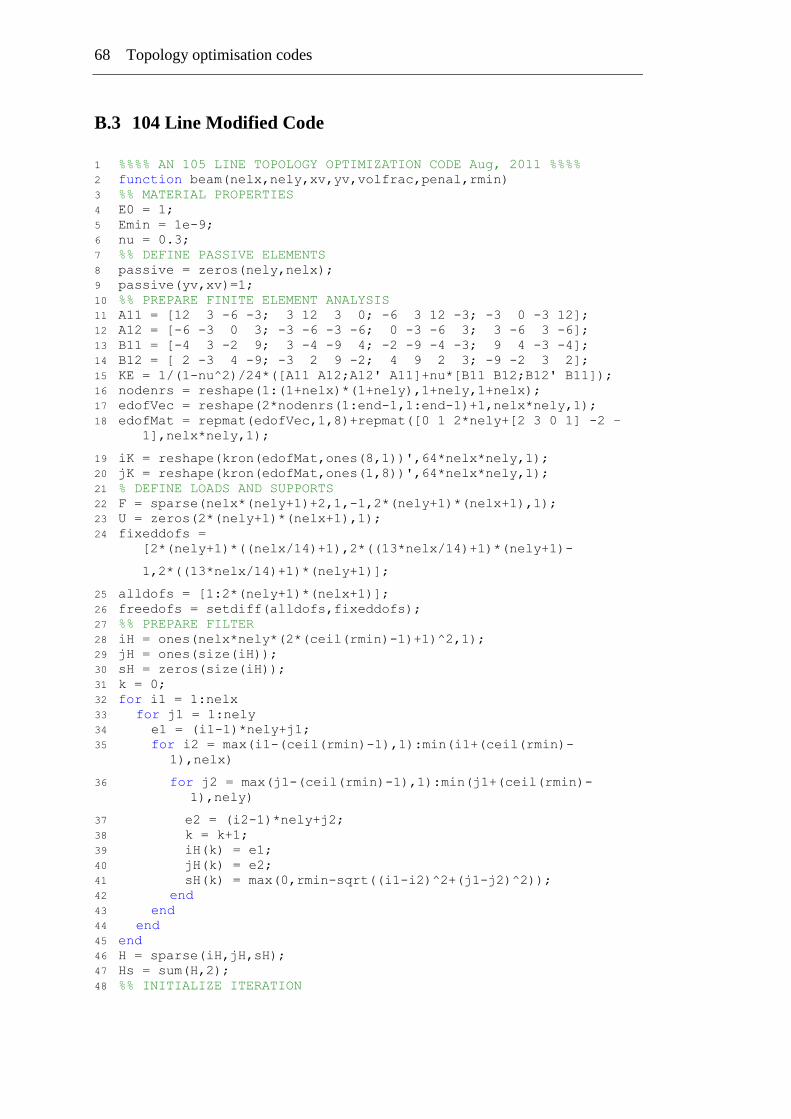
68 Topology optimisation codes
B.3 104 Line Modified Code
1 %%%% AN 105 LINE TOPOLOGY OPTIMIZATION CODE Aug, 2011 %%%% 2 function beam(nelx,nely,xv,yv,volfrac,penal,rmin) 3 %% MATERIAL PROPERTIES 4 E0 = 1; 5 Emin = 1e-9; 6 nu = 0.3; 7 %% DEFINE PASSIVE ELEMENTS 8 passive = zeros(nely,nelx); 9 passive(yv,xv)=1; 10 %% PREPARE FINITE ELEMENT ANALYSIS 11 A11 = [12 3 -6 -3; 3 12 3 0; -6 3 12 -3; -3 0 -3 12]; 12 A12 = [-6 -3 0 3; -3 -6 -3 -6; 0 -3 -6 3; 3 -6 3 -6]; 13 B11 = [-4 3 -2 9; 3 -4 -9 4; -2 -9 -4 -3; 9 4 -3 -4]; 14 B12 = [ 2 -3 4 -9; -3 2 9 -2; 4 9 2 3; -9 -2 3 2]; 15 KE = 1/(1-nu^2)/24*([A11 A12;A12' A11]+nu*[B11 B12;B12' B11]); 16 nodenrs = reshape(1:(1+nelx)*(1+nely),1+nely,1+nelx); 17 edofVec = reshape(2*nodenrs(1:end-1,1:end-1)+1,nelx*nely,1); 18 edofMat = repmat(edofVec,1,8)+repmat([0 1 2*nely+[2 3 0 1] -2 –
1],nelx*nely,1);
19 iK = reshape(kron(edofMat,ones(8,1))',64*nelx*nely,1); 20 jK = reshape(kron(edofMat,ones(1,8))',64*nelx*nely,1); 21 % DEFINE LOADS AND SUPPORTS 22 F = sparse(nelx*(nely+1)+2,1,-1,2*(nely+1)*(nelx+1),1); 23 U = zeros(2*(nely+1)*(nelx+1),1); 24 fixeddofs =
[2*(nely+1)*((nelx/14)+1),2*((13*nelx/14)+1)*(nely+1)-
1,2*((13*nelx/14)+1)*(nely+1)];
25 alldofs = [1:2*(nely+1)*(nelx+1)]; 26 freedofs = setdiff(alldofs,fixeddofs); 27 %% PREPARE FILTER 28 iH = ones(nelx*nely*(2*(ceil(rmin)-1)+1)^2,1); 29 jH = ones(size(iH)); 30 sH = zeros(size(iH)); 31 k = 0; 32 for i1 = 1:nelx 33 for j1 = 1:nely 34 e1 = (i1-1)*nely+j1; 35 for i2 = max(i1-(ceil(rmin)-1),1):min(i1+(ceil(rmin)-
1),nelx)
36 for j2 = max(j1-(ceil(rmin)-1),1):min(j1+(ceil(rmin)- 1),nely)
37 e2 = (i2-1)*nely+j2; 38 k = k+1; 39 iH(k) = e1; 40 jH(k) = e2; 41 sH(k) = max(0,rmin-sqrt((i1-i2)^2+(j1-j2)^2)); 42 end 43 end 44 end 45 end 46 H = sparse(iH,jH,sH); 47 Hs = sum(H,2); 48 %% INITIALIZE ITERATION
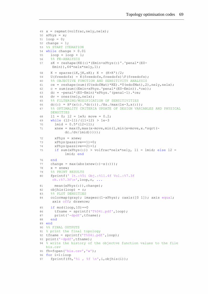
Topology optimisation codes 69
49 x = repmat(volfrac,nely,nelx); 50 xPhys = x; 51 loop = 0; 52 change = 1; 53 %% START ITERATION 54 while change > 0.01 55 loop = loop + 1; 56 %% FE-ANALYSIS 57 sK = reshape(KE(:)*(Emin+xPhys(:)'.^penal*(E0-
Emin)),64*nelx*nely,1);
58 K = sparse(iK,jK,sK); K = (K+K')/2; 59 U(freedofs) = K(freedofs,freedofs)\F(freedofs); 60 %% OBJECTIVE FUNCTION AND SENSITIVITY ANALYSIS 61 ce = reshape(sum((U(edofMat)*KE).*U(edofMat),2),nely,nelx); 62 c = sum(sum((Emin+xPhys.^penal*(E0-Emin)).*ce)); 63 dc = -penal*(E0-Emin)*xPhys.^(penal-1).*ce; 64 dv = ones(nely,nelx); 65 %% FILTERING/MODIFICATION OF SENSITIVITIES 66 dc(:) = H*(x(:).*dc(:))./Hs./max(1e-3,x(:)); 67 %% OPTIMALITY CRITERIA UPDATE OF DESIGN VARIABLES AND PHYSICAL
DENSITIES 68 l1 = 0; l2 = 1e9; move = 0.2; 69 while (l2-l1)/(l1+l2) > 1e-3 70 lmid = 0.5*(l2+l1); 71 xnew = max(0,max(x-move,min(1,min(x+move,x.*sqrt(-
dc./dv/lmid)))));
72 xPhys = xnew; 73 xPhys(passive==1)=0; 74 xPhys(passive==2)=1; 75 if sum(xPhys(:)) > volfrac*nelx*nely, l1 = lmid; else l2 =
lmid; end
76 end 77 change = max(abs(xnew(:)-x(:))); 78 x = xnew; 79 %% PRINT RESULTS 80 fprintf(' It.:%5i Obj.:%11.4f Vol.:%7.3f
ch.:%7.3f\n',loop,c, ...
81 mean(xPhys(:)),change); 82 objhis(loop) = c; 83 %% PLOT DENSITIES 84 colormap(gray); imagesc(1-xPhys); caxis([0 1]); axis equal;
axis off; drawnow;
85 if mod(loop,10)==0 86 tfname = sprintf('T%04i.pdf',loop); 87 print('-dpdf',tfname); 88 end 89 end 90 %% FINAL OUTPUTS 91 % print the final topology 92 tfname = sprintf('T%04i.pdf',loop); 93 print('-dpdf',tfname); 94 % write the history of the objectve function values to the file
his.csv 95 fh=fopen('his.csv','w'); 96 for i=1:loop 97 fprintf(fh,'%i , %f \n',i,objhis(i));

70 Topology optimisation codes
98 end 99 fclose(fh); 100 % plot the evolution of the objective function and print it to
his.pdf 101 figure; 102 plot(1:loop,objhis,'r','LineWidth',2); 103 ylabel('objective function'); xlabel('Iteration'); 104 print('-dpdf','his.pdf');
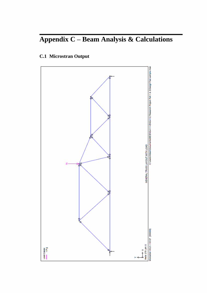
Appendix C – Beam Analysis & Calculations
C.1 Microstran Output
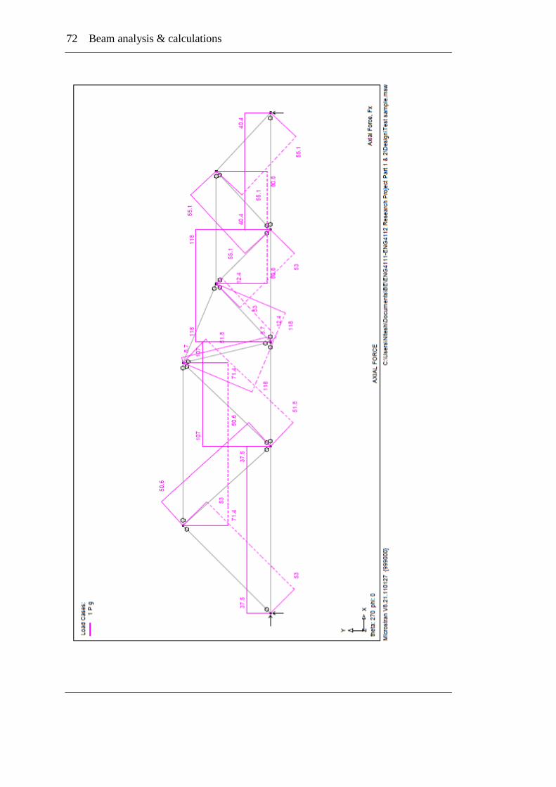
72 Beam analysis & calculations
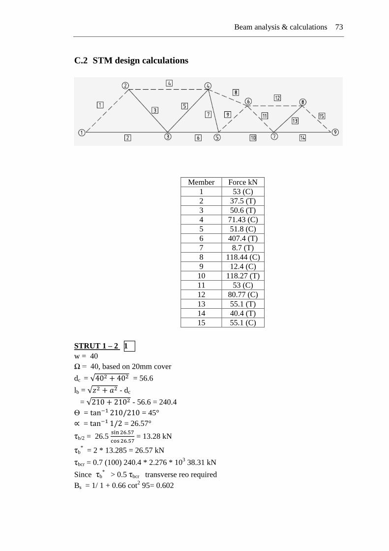
Beam analysis & calculations 73
C.2 STM design calculations
Member Force kN
1 53 (C)
2 37.5 (T)
3 50.6 (T)
4 71.43 (C)
5 51.8 (C)
6 407.4 (T)
7 8.7 (T)
8 118.44 (C)
9 12.4 (C)
10 118.27 (T)
11 53 (C)
12 80.77 (C)
13 55.1 (T)
14 40.4 (T)
15 55.1 (C)
STRUT 1 – 2 1
w = 40
Ω = 40, based on 20mm cover
dc = = 56.6
lb = - dc
= - 56.6 = 240.4
Ѳ = = 45°
= = 26.57°
τb/2 = 26.5
= 13.28 kN
τb* = 2 * 13.285 = 26.57 kN
τbcr = 0.7 (100) 240.4 * 2.276 * 103 38.31 kN
Since τb* > 0.5 τbcr transverse reo required
Bs = 1/ 1 + 0.66 cot2 95= 0.602
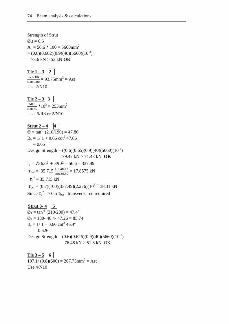
74 Beam analysis & calculations
Strength of Strut
Øst = 0.6
Ac = 56.6 * 100 = 5660mm2
= (0.6)(0.602)(0.9)(40)(5660)(10-3
)
= 73.6 kN > 53 kN OK
Tie 1 – 3 2
= 93.75mm
2 = Ast
Use 2/N10
Tie 2 – 3 3
*10
3 = 253mm
2
Use 5/R8 or 2/N10
Strut 2 – 4 4
Θ = tan-1
(210/190) = 47.86
Bb = 1/ 1 + 0.66 cot2 47.86
= 0.65
Design Strength = ((0.6)(0.65)(0.9)(40)(5660)(10-3
)
= 79.47 kN > 71.43 kN OK
lb = – 56.6 = 337.49
τb/2 = 35.715
= 17.8575 kN
τb* = 35.715 kN
τbcr = (0.7)(100)(337.49)(2.276)(103) =
38.31 kN
Since τb* > 0.5 τbcr transverse reo required
Strut 3- 4 5
Ø1 = tan-1
(210/200) = 47.4°
Ø2 = 180- 46.4- 47.26 = 85.74
Bs = 1/ 1 + 0.66 cot2 46.4°
= 0.626
Design Strength = (0.6)(0.626)(0.9)(40)(5660)(10-3
)
= 76.48 kN > 51.8 kN OK
Tie 3 – 5 6
107.1/ (0.8)(500) = 267.75mm2 = Ast
Use 4/N10
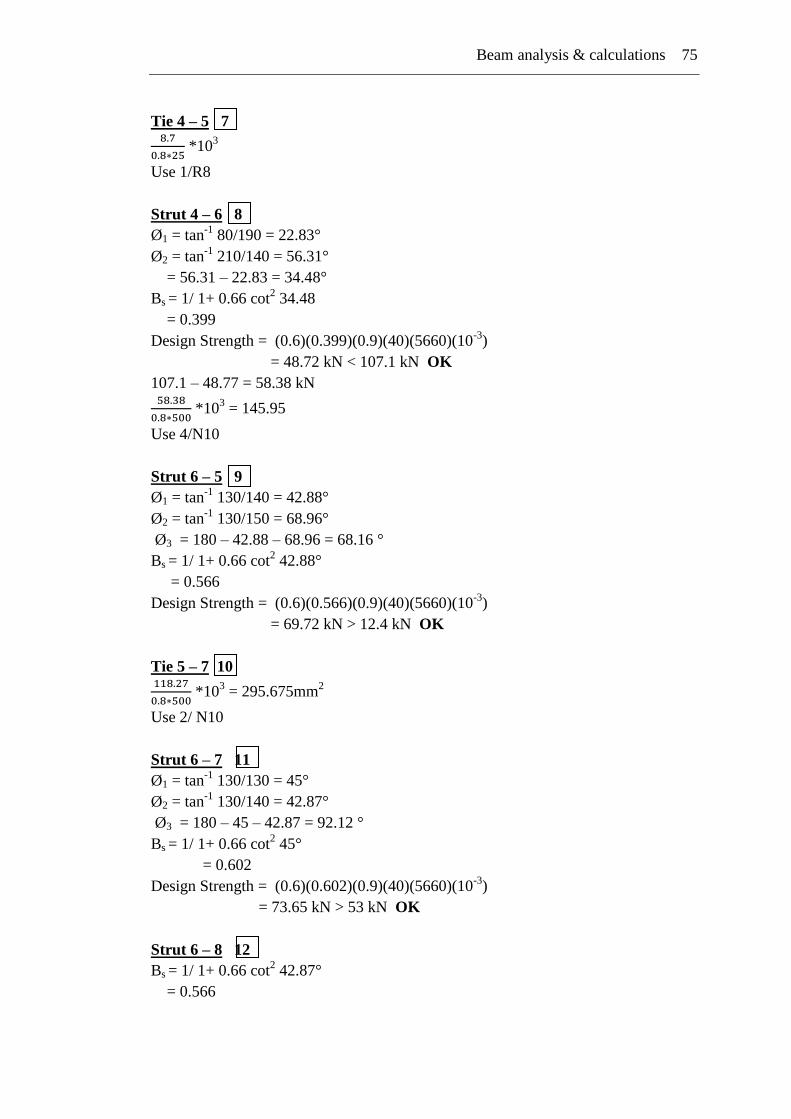
Beam analysis & calculations 75
Tie 4 – 5 7
*10
3
Use 1/R8
Strut 4 – 6 8
Ø1 = tan-1
80/190 = 22.83°
Ø2 = tan-1
210/140 = 56.31°
= 56.31 – 22.83 = 34.48°
Bs = 1/ 1+ 0.66 cot2 34.48
= 0.399
Design Strength = (0.6)(0.399)(0.9)(40)(5660)(10-3
)
= 48.72 kN < 107.1 kN OK
107.1 – 48.77 = 58.38 kN
*10
3 = 145.95
Use 4/N10
Strut 6 – 5 9
Ø1 = tan-1
130/140 = 42.88°
Ø2 = tan-1
130/150 = 68.96°
Ø3 = 180 – 42.88 – 68.96 = 68.16 °
Bs = 1/ 1+ 0.66 cot2 42.88°
= 0.566
Design Strength = (0.6)(0.566)(0.9)(40)(5660)(10-3
)
= 69.72 kN > 12.4 kN OK
Tie 5 – 7 10
*10
3 = 295.675mm
2
Use 2/ N10
Strut 6 – 7 11
Ø1 = tan-1
130/130 = 45°
Ø2 = tan-1
130/140 = 42.87°
Ø3 = 180 – 45 – 42.87 = 92.12 °
Bs = 1/ 1+ 0.66 cot2 45°
= 0.602
Design Strength = (0.6)(0.602)(0.9)(40)(5660)(10-3
)
= 73.65 kN > 53 kN OK
Strut 6 – 8 12
Bs = 1/ 1+ 0.66 cot2 42.87°
= 0.566

76 Beam analysis & calculations
Design Strength = (0.6)(0.566)(0.9)(40)(5660)(10-3
)
= 69.25 kN < 82.77 kN OK
80.71 – 69.25 = 11.52kN
*10
3 = 57.6
Use 2/ R8
Tie 7 – 8 13
*10
3 = 137.75mm
2
Use 2/ N10
Tie 7 – 9 14
*10
3 = 101mm
2
Use 2/ N10
Strut 8 – 9 15
Ø = tan-1
130/140 = 42.88°
Bs = 1/ 1+ 0.66 cot2 42.88°
= 0.566
Design Strength = (0.6)(0.566)(0.9)(40)(5660)(10-3
)
= 69.25 kN > 55.1 kN OK
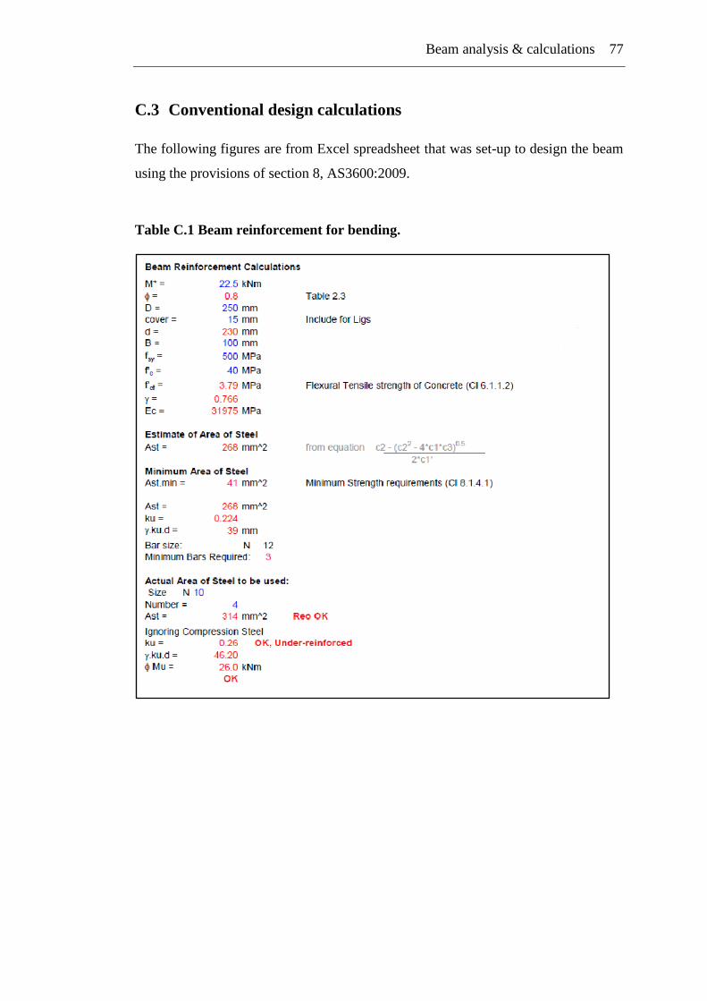
Beam analysis & calculations 77
C.3 Conventional design calculations
The following figures are from Excel spreadsheet that was set-up to design the beam
using the provisions of section 8, AS3600:2009.
Table C.1 Beam reinforcement for bending.

78 Beam analysis & calculations
Table C.2 Shear reinforcement at right end of beam (250mm depth)
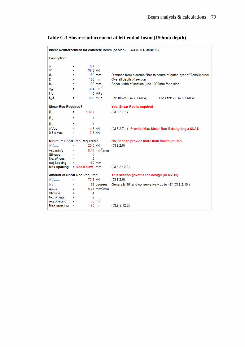
Beam analysis & calculations 79
Table C.3 Shear reinforcement at left end of beam (150mm depth)
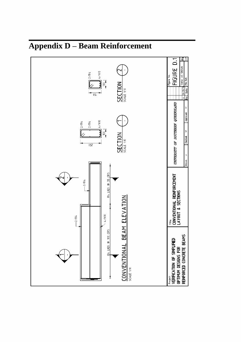
Appendix D – Beam Reinforcement
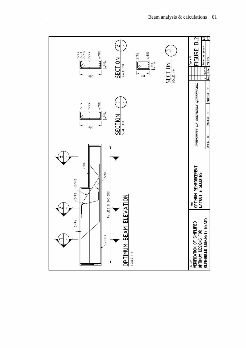
Beam analysis & calculations 81
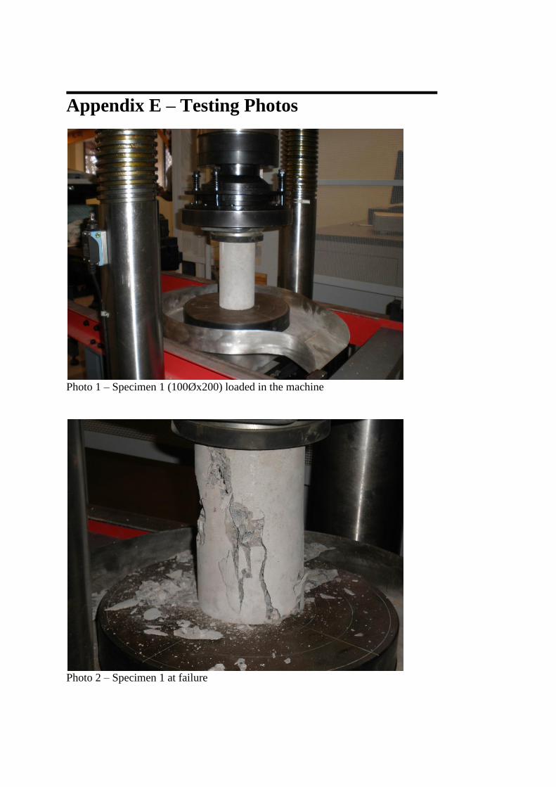
Appendix E – Testing Photos
Photo 1 – Specimen 1 (100Øx200) loaded in the machine
Photo 2 – Specimen 1 at failure
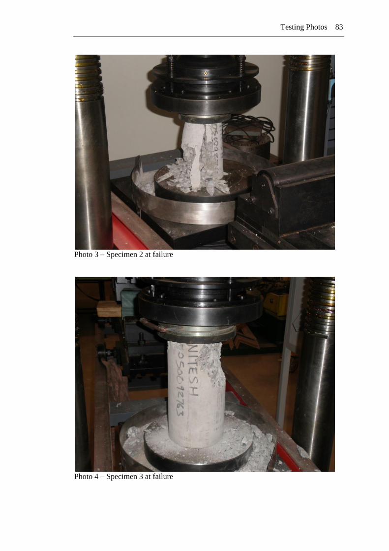
Testing Photos 83
Photo 3 – Specimen 2 at failure
Photo 4 – Specimen 3 at failure
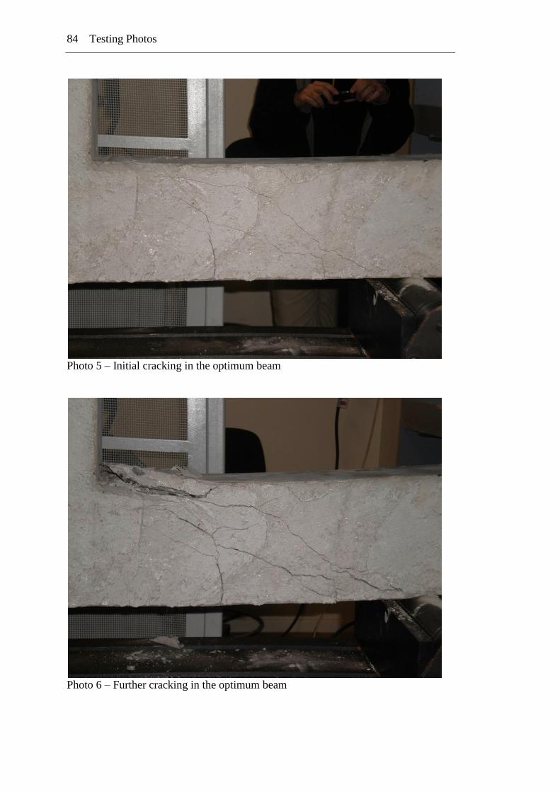
84 Testing Photos
Photo 5 – Initial cracking in the optimum beam
Photo 6 – Further cracking in the optimum beam
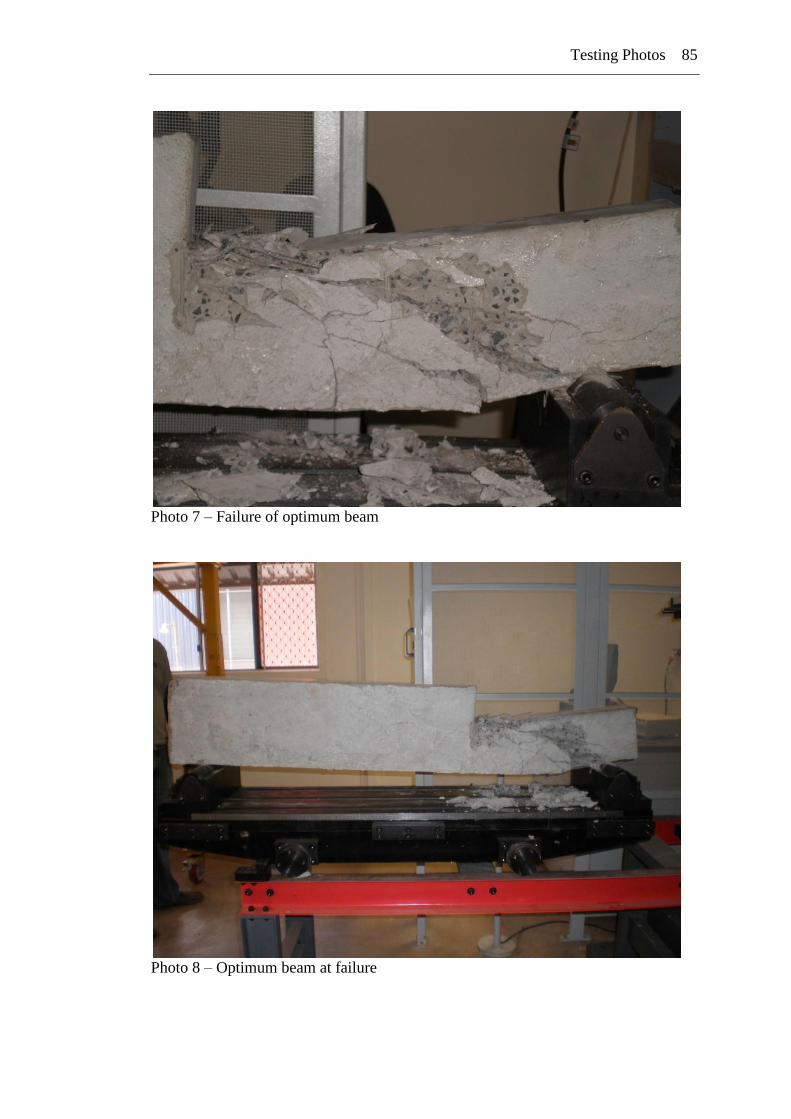
Testing Photos 85
Photo 7 – Failure of optimum beam
Photo 8 – Optimum beam at failure
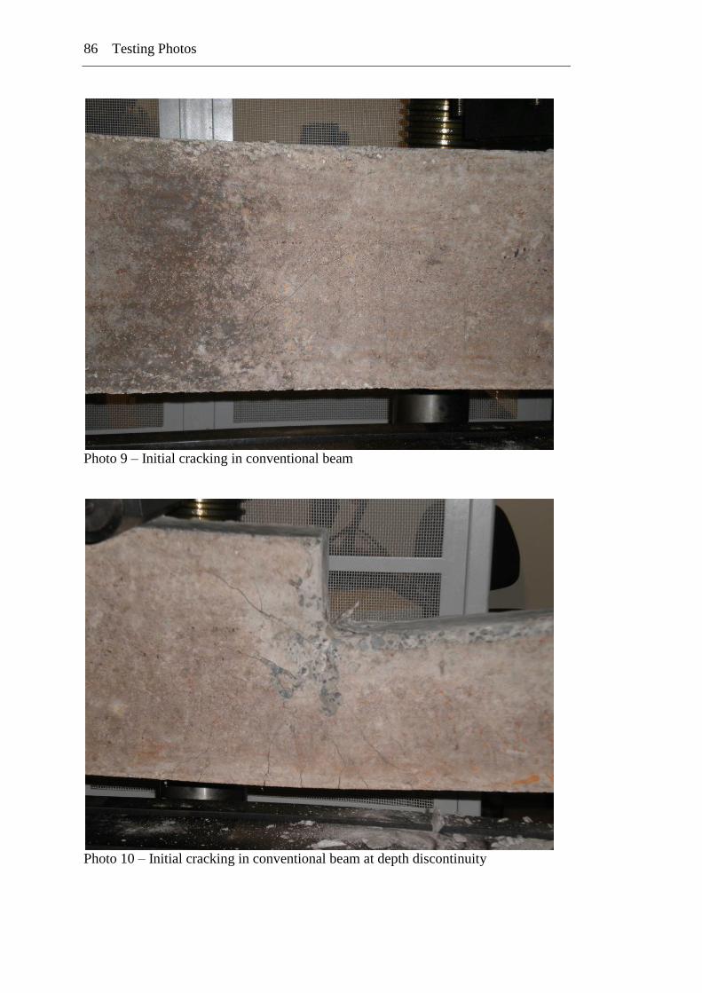
86 Testing Photos
Photo 9 – Initial cracking in conventional beam
Photo 10 – Initial cracking in conventional beam at depth discontinuity
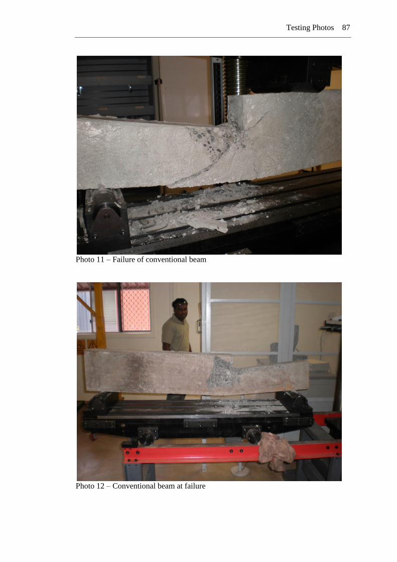
Testing Photos 87
Photo 11 – Failure of conventional beam
Photo 12 – Conventional beam at failure