Embed Size (px)
Citation preview

Ala
ska
Dep
artm
ent o
f Tra
nsp
orta
tion
& P
ub
lic Fa
cilities
Ala
ska U
niv
ersity T
ran
sporta
tion
Cen
ter
Verification of Job Mix Formula for Alaskan
HMA
DOT&PF Report Number 400085INE/ AUTC 14.11
Peng Li, Ph.D. Research Assistant
Jenny Liu, Ph.D. P.E. Associate Professor
Department of Civil and Environmental Engineering
University of Alaska Fairbanks
August 2014
Alaska University Transportation Center
Duckering Building Room 245
P.O. Box 755900
Fairbanks, AK 99775-5900
Alaska Department of Transportation
Research, Development, and Technology
Transfer
2301 Peger Road
Fairbanks, AK 99709-5399

REPORT DOCUMENTATION PAGE
Form approved OMB No.
Public reporting for this collection of information is estimated to average 1 hour per response, including the time for reviewing instructions, searching existing data sources, gathering and
maintaining the data needed, and completing and reviewing the collection of information. Send comments regarding this burden estimate or any other aspect of this collection of information,
including suggestion for reducing this burden to Washington Headquarters Services, Directorate for Information Operations and Reports, 1215 Jefferson Davis Highway, Suite 1204, Arlington,
VA 22202-4302, and to the Office of Management and Budget, Paperwork Reduction Project (0704-1833), Washington, DC 20503
1. AGENCY USE ONLY (LEAVE BLANK)
DOT&PF Report Number 4000085
2. REPORT DATE
August 2014
3. REPORT TYPE AND DATES COVERED
Final Report (August 2009 – January 2012)
4. TITLE AND SUBTITLE
Verification of Job Mix Formula for Alaskan HMA
5. FUNDING NUMBERS
Alaska DOT&PF: T2-09-08
AKSAS 63271
AUTC: 309024 6. AUTHOR(S)
Peng Li, Ph.D., Research Assistant
Jenny Liu, Ph.D., P.E., Associate Professor
7. PERFORMING ORGANIZATION NAME(S) AND ADDRESS(ES)
Alaska University Transportation Center
University of Alaska Fairbanks
Duckering Building Room 245
P.O. Box 755900
Fairbanks, AK 99775-5900
8. PERFORMING ORGANIZATION REPORT
NUMBER
INE/AUTC 14.11
9. SPONSORING/MONITORING AGENCY NAME(S) AND ADDRESS(ES)
State of Alaska, Alaska Dept. of Transportation and Public Facilities
Research and Technology Transfer
2301 Peger Rd
Fairbanks, AK 99709-5399
10. SPONSORING/MONITORING AGENCY
REPORT NUMBER
DOT&PF Report Number 4000085
11. SUPPLENMENTARY NOTES
Performed in cooperation with the Alaska Department of Transportation and Public Facilities Materials Section
12a. DISTRIBUTION / AVAILABILITY STATEMENT
No restrictions
12b. DISTRIBUTION CODE
13. ABSTRACT (Maximum 200 words)
Some asphalt pavement does not last as long as it should. Every year, a significant amount of money is spent by the state on
repairing and maintaining pavement, which raises the question: Are we getting the mix design we need? Since hot mix asphalt (HMA) is
the main paving material in Alaska, it is critical to understand how the quality of this material is assured. Often, a properly lab-designed
HMA is used in the field on a given project and performs in a substandard manner. Variability is inevitable during construction.
Two projects were selected for the study. Pertinent data from ADOT&PF and from contractors at lab/design and construction
were obtained, including general information regarding the paving projects, details of the materials and JMF being used in the
construction, quality control testing data from contractors, and acceptance testing results from the agency.
14- KEYWORDS : Asphalt Tests (Gbbmd), Asphalt concrete pavement (Pmrcppbmd), asphalt plants (Pfkpb), hot mix asphalt
(Rbmuejph)
15. NUMBER OF PAGES
101 16. PRICE CODE
N/A 17. SECURITY CLASSIFICATION OF REPORT
Unclassified
18. SECURITY CLASSIFICATION OF THIS PAGE
Unclassified
19. SECURITY CLASSIFICATION OF ABSTRACT
Unclassified
20. LIMITATION OF ABSTRACT
N/A
NSN 7540-01-280-5500 STANDARD FORM 298 (Rev. 2-98) Prescribed by ANSI Std. 239-18 298-

iii
Notice
This document is disseminated under the sponsorship of the U.S. Department of
Transportation in the interest of information exchange. The U.S. Government assumes no
liability for the use of the information contained in this document. The U.S. Government
does not endorse products or manufacturers. Trademarks or manufacturers’ names appear
in this report only because they are considered essential to the objective of the document.
Quality Assurance Statement
The Federal Highway Administration (FHWA) provides high-quality information to
serve Government, industry, and the public in a manner that promotes public
understanding. Standards and policies are used to ensure and maximize the quality,
objectivity, utility, and integrity of its information. FHWA periodically reviews quality
issues and adjusts its programs and processes to ensure continuous quality improvement.
Author’s Disclaimer
Opinions and conclusions expressed or implied in the report are those of the author. They
are not necessarily those of the Alaska DOT&PF or funding agencies.

iv
Abstract
Some asphalt pavement does not last as long as it should. Every year, a significant amount of
money is spent by the state on repairing and maintaining pavement, which raises the question:
Are we getting the mix design we need? Since hot mix asphalt (HMA) is the main paving
material in Alaska, it is critical to understand how the quality of this material is assured. Often, a
properly lab-designed HMA is used in the field on a given project and performs in a substandard
manner. Variability is inevitable during construction.
Two projects were selected for the study. Pertinent data from ADOT&PF and from contractors at
lab/design and construction were obtained, including general information regarding the paving
projects, details of the materials and JMF being used in the construction, quality control testing
data from contractors, and acceptance testing results from the agency.

v
ACKNOWLEDGMENTS
The authors wish to express their appreciation to personnel at the Alaska Department of
Transportation and Public Facilities and the Alaska University Transportation Center for their
support throughout this study. The authors would also like to thank all members of the project
advisory committee.

vi
EXECUTIVE SUMMARY
Some asphalt pavement does not last as long as it should. Every year, a significant
amount of money is spent by the state on repairing and maintaining pavement, which raises the
question: Are we getting the mix design we need? Since hot mix asphalt (HMA) is the main
paving material in Alaska, it is critical to understand how the quality of this material is assured.
Often, a properly lab-designed HMA is used in the field on a given project and performs
in a substandard manner. Variability is inevitable during construction. An ongoing National
Cooperative Highway Research Program (NCHRP) study (Mohammad and Elseifi 2010) is
investigating field-versus-laboratory volumetrics and mechanical properties in an effort to
quantify variabilities and ensure sound quality assurance and pavement design approaches.
No research has been focused on the performance of HMA mixtures with respect to
material types and climatic conditions typical of Alaska. Previous material quality assurance
(QA) reviews of the Alaska Department of Transportation and Public Facilities (ADOT&PF),
conducted by the Federal Highway Administration (FHWA), provided recommendations for
improvement, such as transitioning to the Superpave mix design as standard practice, and
moving away from the use of gradation as acceptance criteria, accepting asphalt mixes based on
volumetric properties instead. To respond to the FHWA’s comments and facilitate satisfactory
construction of HMA pavements, a comprehensive study on field data collection, compilation,
and analysis was conducted to investigate the variability of HMA performance due to production,
and to verify the HMA job mix formula (JMF). The study is presented in this report.
Two asphalt paving projects—the Parks Highway Mile 287–305 rehabilitation and
resurface project and the Anchorage International Airport (AIA) runway 7R/25L rehabilitation—
were selected for fieldwork. Pertinent data from ADOT&PF and from contractors at lab/design
and construction were obtained, including general information regarding the paving projects,
details of the materials and JMF being used in the construction, quality control testing data from
contractors, and acceptance testing results from the agency. To evaluate the variability of HMA
involved in the construction process and the impact on its performance, specimens of four
scenarios were prepared from these two paving projects: (1) specimens mixed and compacted in
the laboratory using the same JMF (L&L), (2) loose mixtures collected from the windrow and
compacted in the field (F&F), (3) loose mixtures collected from the windrow and compacted in
the laboratory (F&L), and (4) cores retrieved from the field after paving. Three types of HMA
properties were measured:
Composition properties: gradation and binder content.
Volumetric properties: voids in the total mix (VTM), voids in the mineral aggregate
(VMA), and voids filled with asphalt (VFA).

vii
Mechanical properties: dynamic modulus (│E*│), creep stiffness, and indirect tensile
strength (ITS).
Composition properties were measured on F&F and F&L scenarios. Because the L&L
specimens were prepared on laboratory-blend mixtures according to the JMF, the gradation and
binder content tests were not needed. Volumetric properties were evaluated on at least three
replicates of specimens prepared from all four scenarios. Dynamic modulus and flow tests were
only performed on L&L and F&L specimens due to the large sample size required for testing.
Indirect tensile (IDT) creep tests were performed for all four scenarios at three testing
temperatures: -10°C, -20°C, and -30°C. For L&L and F&L specimens, the ITS tests were
performed at three temperatures as well: -10°C, -20°C, and -30°C. Due to the limited numbers of
F&F specimens and field cores, the ITS tests were only performed at -20°C for field cores and at
-10°C and -30°C for F&F specimens.
Among the three types of properties tested, mechanical properties had the greatest sublot-
wise variance. Generally, the observed variances were close to those of previous studies and
within the limits recommended by AASHTO R42. The variance of percentage passing of
aggregate at different sieve size was less than 2.5%, though the extreme value reached 4.5%. The
variance of binder contents was less than 0.25%. The variance of aggregate gradation was
significantly affected by operator and sublot number. The statistical analysis indicates that the
binder content was stable during the material production, but the data obtained using the ignition
method varied among operators. The differences in volumetric properties between JMF and the
specimens prepared from the four scenarios were observed. It was found that the differences are
significantly affected by sublot and scenario. The variance of volumetric properties was only
affected by testing scenario, that is, L&L, F&L, F&F, and field cores. The highest standard
deviations (STDEVs) of VTM, VMA, and VFA were 1.4, 1.2, and 6.7, respectively.
The variations of composition properties, as measured by coefficient of variance (COV),
were found to be approximately 5%. The COVs of volumetric properties ranged from 2% to 14%.
The variations of mechanical properties were much higher than composition and volumetric
properties. Among all mechanical properties investigated, ITS had the lowest COV (7%), and
flow tests had the highest COV (up to 43%). The │E*│ of field-produced HMA was greatly
affected by material production and testing conditions. The results of a multi-factor ANOVA
analysis indicate that frequency, sublot, and temperature are significant factors. The variance of
│E*│ was affected by sublot and temperature. Generally, creep stiffness obtained from three
field scenarios—F&L, F&F, and field cores—differed from the value of L&L specimens. The
percentage errors were significantly affected by scenario, sublot, temperature, and loading time.
The variance of creep stiffness was not influenced by these factors. The results of ITS revealed a
difference between field scenarios and the L&L scenario, which also changed during the

viii
production of HMA. The ITS testing results had the lowest variance among all mechanical
properties.
The variances of mechanical properties were higher than those of both composition and
volumetric properties. The reason for this could be that additional errors were introduced during
specimen cutting, sensor installation, and loading, activities not required for composition and
volumetric properties. Previous studies from others (Bonaquist 2008) confirmed this observation.
The correlations between composition and mechanical properties and between volumetric
and mechanical properties were evaluated. Although volumetric properties provide a better
correlation with mechanical properties than with composition properties, as indicated by higher
R2 values, the correlation was generally found to be weak.
The purpose of a QA program is to improve the quality of HMA mixtures and to make
the best effort in ensuring that the performance of installed HMA mixtures reaches the levels
specified in the design. Rather than measuring mechanical properties, which are considered
directly related to pavement performance, composition and/or volumetric properties are
measured in most QA programs. They are preferred because composition and volumetric
properties can be measured easier and faster than mechanical properties, and fewer variations are
introduced, as indicated by this study. However, the statistical analyses and results of this study
were based on limited data collected from only two paving projects. More data from various
paving projects are recommended to further confirm and validate the findings reported here.

ix
TABLE OF CONTENTS
EXECUTIVE SUMMARY ........................................................................................................... vi
LIST OF FIGURES ....................................................................................................................... xi
LIST OF TABLES ....................................................................................................................... xiv
CHAPTER 1 INTRODUCTION .................................................................................................... 1
1.1 Problem Statement ................................................................................................................ 1
1.2 Objectives ............................................................................................................................. 1
1.3 Research Methodology ......................................................................................................... 2
CHAPTER 2 LITERATURE REVIEW ......................................................................................... 4
2.1 Types of Quality Assurance Specification ............................................................................ 4
2.2 Key Material Characteristics and Influencing Factors of HMA ........................................... 6
2.2.1 Key Material Characteristics .......................................................................................... 6
2.2.2 Influencing Factors ...................................................................................................... 12
CHAPTER 3 FIELD AND LABORATORY TESTS .................................................................. 16
3.1 Fieldwork Plan .................................................................................................................... 16
3.2 Experimental Design ........................................................................................................... 18
3.3 Specimen Fabrication.......................................................................................................... 19
3.4 Laboratory Testing .............................................................................................................. 21
3.4.1 Composition Properties ................................................................................................ 21
3.4.2 Volumetric Properties .................................................................................................. 22
3.4.3 Mechanical Properties .................................................................................................. 22
3.4.4 Indirect Tensile (IDT) Tests ......................................................................................... 23
CHAPTER 4 TESTING RESULTS AND DATA ANALYSIS ................................................... 25
4.1 Composition Properties ....................................................................................................... 25
4.1.1 Testing Results ............................................................................................................. 25
4.1.2 Analysis of Variance .................................................................................................... 30
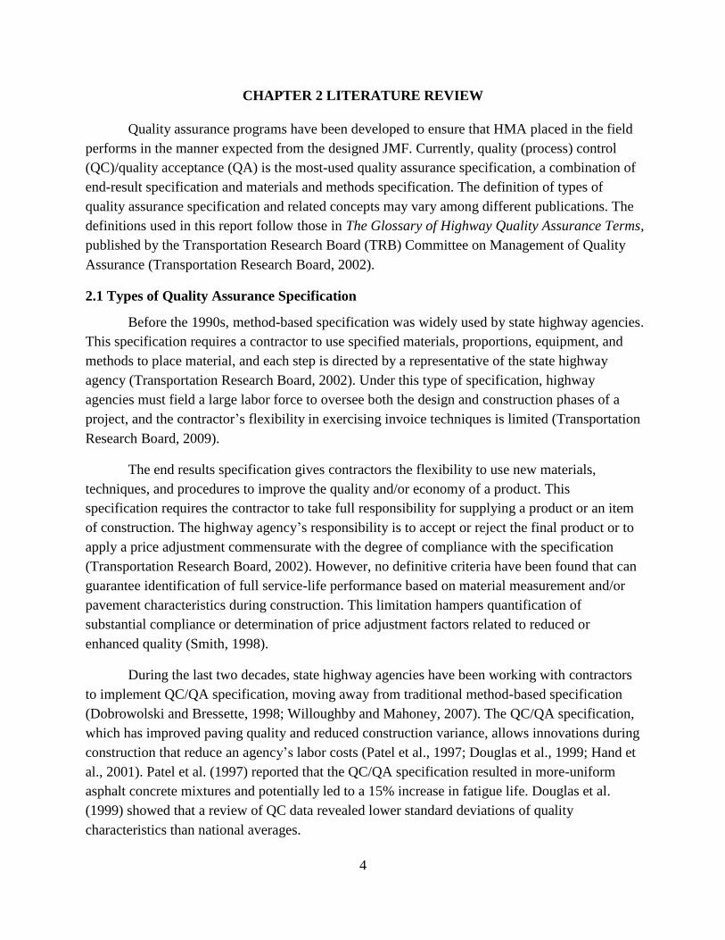
4.1.3 Analysis of Error .......................................................................................................... 32
4.2 Volumetric Properties ......................................................................................................... 39
4.2.1 Testing Result .............................................................................................................. 39
4.2.2 Analysis of Variance .................................................................................................... 41

x
4.2.3 Analysis of Error .......................................................................................................... 43
4.3 Mechanical Properties ......................................................................................................... 46
4.3.1 Dynamic Modulus ........................................................................................................ 46
4.3.2 Flow Test ..................................................................................................................... 55
4.3.3 Creep Stiffness ............................................................................................................. 58
4.3.4 Indirect Tensile Strength .............................................................................................. 67
4.4 Correlation .......................................................................................................................... 73
CHAPTER 5 CONCLUSIONS .................................................................................................... 76
REFERENCES ............................................................................................................................. 78
Appendix A Summary of Volumetric Properties Results ............................................................. 83
Appendix B Summary of Dynamic Modulus Results ................................................................... 84
Appendix C Summary of Flow Test Results ................................................................................ 86
Appendix D Summary of IDT Creep Test Results ....................................................................... 87
Appendix E Summary of Flow Test Results................................................................................. 88

xi
LIST OF FIGURES
Figure 2.1 Quality characteristics used by state highway agency (SHA) ........................................7
Figure 2.2 Summary of number of quality characteristics used by SHA for QC/QA .....................7
Figure 3.1 Field sampling procedures ............................................................................................20
Figure 3.2 Field lab for AIA paving project ..................................................................................21
Figure 3.3 Setup of the asphalt mixture performance tester (AMPT) ...........................................22
Figure 3.4 Setup for indirect tensile (IDT) test ..............................................................................24
Figure 4.1 Gradation chart of AIA paving project .........................................................................27
Figure 4.2 Gradation chart of Nenana paving project....................................................................29
Figure 4.3 Binder content ..............................................................................................................29
Figure 4.4 Variance of sieving analysis .........................................................................................30
Figure 4.5 Standard deviation of sieving analysis from three operators ........................................31
Figure 4.6 Variation of binder content ...........................................................................................32
Figure 4.7 Difference between measured and design values (1/2″ sieve) .....................................33
Figure 4.8 Difference between measured and design values (3/8″ sieve) .....................................33
Figure 4.9 Difference between measured and design values (#4 sieve) ........................................34
Figure 4.10 Difference between measured and design values (#8 sieve) ......................................34
Figure 4.11 Difference between measured and design values (#16 sieve) ....................................35
Figure 4.12 Difference between measured and design values (#30 sieve) ....................................35
Figure 4.13 Difference between measured and design values (#50 sieve) ....................................36
Figure 4.14 Difference between measured and design values (#100 sieve) ..................................36
Figure 4.15 Difference between measured and design values (#200 sieve) ..................................37
Figure 4.16 Difference between measured and design values (binder content) ............................37
Figure 4.17 Summary of percent air voids of total mix .................................................................40
Figure 4.18 Summary of percent void in mineral aggregate .........................................................40
Figure 4.19 Summary of percent voids filled with asphalt binder .................................................41
Figure 4.20 Standard deviation of VTM from three scenarios ......................................................42
Figure 4.21 Standard deviation of VMA from three scenarios ......................................................42
Figure 4.22 Standard deviation of VFA from three scenarios .......................................................43
Figure 4.23 Difference between measured and design values (VTM) ..........................................44

xii
Figure 4.24 Difference between measured and design values (VMA) ..........................................44
Figure 4.25 Difference between measured and design values (VFA) ...........................................45
Figure 4.26 │E*│at 4°C ................................................................................................................47
Figure 4.27 │E*│at 21°C ..............................................................................................................47
Figure 4.28 │E*│at 37°C ..............................................................................................................48
Figure 4.29 │E*│at 54°C ..............................................................................................................48
Figure 4.30 COV of │E*│ at 4°C .................................................................................................49
Figure 4.31 COV of │E*│ at 21°C ...............................................................................................50
Figure 4.32 COV of │E*│ at 37°C ...............................................................................................50
Figure 4.33 COV of │E*│ at 54°C ...............................................................................................51
Figure 4.34 Percentage error of E* (4°C) ......................................................................................52
Figure 4.35 Percentage error of E* (21°C) ....................................................................................53
Figure 4.36 Percentage error of E* (37°C) ....................................................................................53
Figure 4.37 Percentage error of E* (54°C) ....................................................................................54
Figure 4.38 Microstrains at the end of flow tests...........................................................................56
Figure 4.39 COV of flow tests .......................................................................................................57
Figure 4.40 Difference between measured and design value ........................................................58
Figure 4.41 Creep stiffness at 50s (-10°C) ....................................................................................59
Figure 4.42 Creep stiffness at 50s (-20°C) ....................................................................................59
Figure 4.43 Creep stiffness at 50s (-30°C) ....................................................................................60
Figure 4.44 Creep stiffness at 500s (-10°C) ..................................................................................60
Figure 4.45 Creep stiffness at 500s (-20°C) ..................................................................................61
Figure 4.46 Creep stiffness at 50s (-30°C) ....................................................................................61
Figure 4.47 COV of creep stiffness at 50s .....................................................................................62
Figure 4.48 COV of creep stiffness at 50s .....................................................................................63
Figure 4.49 Difference between measured and design value (-10°C, 50s) ....................................64
Figure 4.50 Difference between measured and design value (-20°C, 50s) ....................................64
Figure 4.51 Difference between measured and design value (-30°C, 50s) ....................................65
Figure 4.52 Difference between measured and design value (-10°C, 500s) ..................................65
Figure 4.53 Difference between measured and design value (-20°C, 500s) ..................................66

xiii
Figure 4.54 Difference between measured and design value (-30°C, 500s) ..................................66
Figure 4.55 IDT strength at -10°C .................................................................................................68
Figure 4.56 IDT strength at -20°C .................................................................................................68
Figure 4.57 IDT strength at -30°C .................................................................................................69
Figure 4.58 COV of IDT strength ..................................................................................................70
Figure 4.59 COV of IDT strength ..................................................................................................70
Figure 4.60 COV of IDT strength ..................................................................................................71
Figure 4.61 Difference between measured and design value (-10°C) ...........................................72
Figure 4.62 Difference between measured and design value (-20°C) ...........................................72
Figure 4.63 Difference between measured and design value (-30°C) ...........................................73
Figure 4.64 Summary of COV by quality characteristic ...............................................................74
Figure 4.65 Correlations between composition and mechanical properties ..................................75
Figure 4.66 Correlation between volumetric and mechanical properties ......................................75

xiv
LIST OF TABLES
Table 2.1 Summary of standard deviation for binder content of plant mix lab measured
sample (data of contractor, SHA, and third party were obtained from Mohammad and
Elseifi, 2010) ....................................................................................................................................8
Table 2.2 Summary of standard deviation for aggregate gradation (Mohammad and
Elseifi, 2010) ....................................................................................................................................9
Table 2.3 Summary of standard deviation for volumetric properties (Mohammad and
Elseifi, 2010) ..................................................................................................................................10
Table 2.4 Summary of coefficient of variation for mechanical properties (Mohammad
and Elseifi, 2010) ...........................................................................................................................12
Table 3.1 Job mix formula of AIA and Nenana paving projects ...................................................17
Table 3.2 Experimental design ......................................................................................................18
Table 4.1 Sieving analysis testing results (AIA paving project) ...................................................26
Table 4.2 Sieving analysis testing results (Nenana paving project) ..............................................28
Table 4.3 Single factor ANOVA analysis......................................................................................31
Table 4.4 Summary of errors of composition properties among three operators ..........................38
Table 4.5 Two-factor ANOVA for error of gradation (= 0.05) ..................................................38
Table 4.6 Two-factor ANOVA for error of binder content (= 0.05) ..........................................39
Table 4.7 Multi-factor ANOVA for variance of volumetric properties .........................................43
Table 4.8 Summary of error of volumetric properties ...................................................................45
Table 4.9 Two-factor ANOVA for error of volumetric properties ................................................45
Table 4.10 Multi-factor ANOVA for COV of │E*│ ....................................................................51
Table 4.11 Summary of percentage error of │E*│ .......................................................................54
Table 4.12 Multi-factor ANOVA for percentage error of │E*│ ..................................................55
Table 4.13 Two-factor ANOVA for variance of microstrain at end of flow test ..........................57
Table 4.14 Two-factor ANOVA for percentage error of microstrain at end of flow test ..............58
Table 4.15 Multi-factor ANOVA for COV of creep stiffness .......................................................63
Table 4.16 Multi-factor ANOVA for % error of creep stiffness ...................................................67
Table 4.17 Multi-factor ANOVA for COV of IDT strength .........................................................71
Table 4.18 Multi-factor ANOVA for % error of IDT strength ......................................................73

1
CHAPTER 1 INTRODUCTION
Since hot mix asphalt (HMA) is the main paving material used in Alaska, assurance of its
quality is critical. It is important to assess elements related to HMA quality assurance (QA)
specifications, to evaluate how well contractors meet the requirements of mix designs, and to
revise current mix design protocols and contractor payment methods for asphalt paving in Alaska.
This comprehensive study, an examination of field data collection, compilation, and analysis,
was conducted to investigate the variability of HMA performance due to production and to verify
the HMA job mix formula (JMF).
1.1 Problem Statement
Every year, a significant amount of state money is spent on repairing and maintaining
pavement, partly because of asphalt pavement that fails prematurely. This recurring problem
raises the question: Are we getting the mix design we need?
As HMA is the main paving material used in Alaska, it is critical that the quality of this
material is assured. Some variability in quality is inevitable because tests are performed by
different operators using different equipment and potentially different methods, and specimen
sampling and compaction are not the same. These factors influence the chosen design property
values. Often, a properly lab-designed HMA will be placed in the field for a given project and
perform in a substandard manner. An ongoing National Cooperative Highway Research Program
(NCHRP) study (Mohammad and Elseifi 2010) is investigating field-versus-laboratory
volumetrics and mechanical properties to quantify the variabilities that arise in paving materials
and to ensure sound quality assurance programs and pavement design approaches. Unfortunately,
no research has been focused on the performance of HMA mixtures with respect to the material
types and climatic conditions typical in Alaska.
In previous material QA reviews of the Alaska Department of Transportation and Public
Facilities (ADOT&PF), the Federal Highway Administration (FHWA) made recommendations
for improvement such as using Superpave mix design as a standard practice and moving toward
asphalt acceptance criteria based on volumetric properties instead of gradation. The current study
is an effort to respond properly to FHWA’s comments and facilitate satisfactory construction of
HMA pavements.
1.2 Objectives
The purpose of this research was to investigate how the properties of HMA mixtures vary
due to mixture production, and how production factors affect current mix design and QA
specifications. The following objectives were addressed:
Comparison of volumetric properties of as-built and JMF properties of HMA for
asphalt paving projects.
2
Evaluation of the variability involved in construction processes and the impact of
construction processes on HMA performance.
Investigation of essential causes or significant influencing factors related to
variabilities in HMA performance.
Recommendations regarding current HMA design and QA specifications.
1.3 Research Methodology
The following major tasks were accomplished to achieve the objectives of this study:
Task 1: Literature Review
Task 2: Development of Field Work Plan and Experimental Design
Task 3: Field Data Collection, Specimen Fabrication, and Testing
Task 4: Data Processing and Analyses
Task 5: Project Summary and Conclusions
Task 1: Literature Review
A comprehensive literature review of previous studies and current research efforts and
progress in the area of quality control (QC) and quality assurance was conducted. The purpose of
the review was to gather information on key subjects pertaining to this study such as the current
status of national QA programs, types of material quality characteristics, variance of quality
characteristics associated with construction and testing processes, and influencing factors.
Chapter 2 presents the summary of this task.
Task 2: Development of Field Work Plan and Experimental Design
The fieldwork plan and experimental design were developed based on information
collected from the literature review and on discussions among members of the research team and
ADOT&PF personnel. Two asphalt paving projects—the Parks Highway Mile 287–305
rehabilitation and resurfacing project and the Anchorage International Airport (AIA) runway
7R/25L rehabilitation—were selected for study. To evaluate the variability of HMA used in the
construction process and the impacts on performance of HMA, specimens for use in four
scenarios were prepared from these two paving projects: (1) specimens mixed and compacted in
the laboratory using the same JMF (L&L), (2) loose mixtures collected from the windrow and
compacted in the field (F&F), (3) loose mixtures collected from the windrow and compacted in
the laboratory (F&L), and (4) cores retrieved from the field after paving. Three types of HMA
properties were measured as follows:
Composition properties: gradation and binder content.
Volumetric properties: voids in the total mix (VTM), voids in the mineral aggregate
(VMA), and voids filled with asphalt (VFA).

3
Mechanical properties: dynamic modulus (│E*│), creep stiffness and indirect tensile
strength (ITS).
The details of this task are included in Chapter 3.
Task 3: Field Data Collection, Specimens Fabrication, and Testing
During the process of each paving project, pertinent data from ADOT&PF and the
contractors at lab/design, production, and newly constructed phases were obtained. This included
general information regarding the paving projects, details of the materials and JMF used in the
construction, quality-control testing data from contractors, and acceptance testing results from
the agency. The F&F specimens were prepared in the field, and tested for composition and
volumetric properties. In addition, materials were collected and shipped to the University of
Alaska Fairbanks (UAF) laboratories for preparation of L&L and F&L specimens. Volumetric
and mechanical properties were investigated using specimens from these two scenarios. Cores
retrieved from the field were used to verify volumetric properties of field mixtures and to
conduct indirect tensile (IDT) tests in the laboratory for low-temperature performance evaluation.
The details of laboratory and fieldwork are described in Chapter 3, and testing results are
presented in Chapter 4.
Task 4: Data Processing and Analyses
Compilation and analyses of laboratory and field data were performed under this task.
Variance and error analyses were conducted to measure sources of variation found in material
properties data. The significance of potential influencing factors, such as operator, sublot, and
scenario, was examined. Relationships among composition properties, volumetric properties, and
mechanical properties were established and compared. This task is presented in Chapter 4.
Task 5: Project Summary and Conclusions
Research results and findings were summarized in this task, as provided in Chapter 5.
4
CHAPTER 2 LITERATURE REVIEW
Quality assurance programs have been developed to ensure that HMA placed in the field
performs in the manner expected from the designed JMF. Currently, quality (process) control
(QC)/quality acceptance (QA) is the most-used quality assurance specification, a combination of
end-result specification and materials and methods specification. The definition of types of
quality assurance specification and related concepts may vary among different publications. The
definitions used in this report follow those in The Glossary of Highway Quality Assurance Terms,
published by the Transportation Research Board (TRB) Committee on Management of Quality
Assurance (Transportation Research Board, 2002).
2.1 Types of Quality Assurance Specification
Before the 1990s, method-based specification was widely used by state highway agencies.
This specification requires a contractor to use specified materials, proportions, equipment, and
methods to place material, and each step is directed by a representative of the state highway
agency (Transportation Research Board, 2002). Under this type of specification, highway
agencies must field a large labor force to oversee both the design and construction phases of a
project, and the contractor’s flexibility in exercising invoice techniques is limited (Transportation
Research Board, 2009).
The end results specification gives contractors the flexibility to use new materials,
techniques, and procedures to improve the quality and/or economy of a product. This
specification requires the contractor to take full responsibility for supplying a product or an item
of construction. The highway agency’s responsibility is to accept or reject the final product or to
apply a price adjustment commensurate with the degree of compliance with the specification
(Transportation Research Board, 2002). However, no definitive criteria have been found that can
guarantee identification of full service-life performance based on material measurement and/or
pavement characteristics during construction. This limitation hampers quantification of
substantial compliance or determination of price adjustment factors related to reduced or
enhanced quality (Smith, 1998).
During the last two decades, state highway agencies have been working with contractors
to implement QC/QA specification, moving away from traditional method-based specification
(Dobrowolski and Bressette, 1998; Willoughby and Mahoney, 2007). The QC/QA specification,
which has improved paving quality and reduced construction variance, allows innovations during
construction that reduce an agency’s labor costs (Patel et al., 1997; Douglas et al., 1999; Hand et
al., 2001). Patel et al. (1997) reported that the QC/QA specification resulted in more-uniform
asphalt concrete mixtures and potentially led to a 15% increase in fatigue life. Douglas et al.
(1999) showed that a review of QC data revealed lower standard deviations of quality
characteristics than national averages.

5
The QC/QA specification has three integral components: quality or process control (QC),
acceptance, and independence assurance (IA) (Hughes, 2005). Generally, a contractor is
responsible for QC, while the highway agency is responsible for acceptance of product. The IA
is performed by an independent third party to provide an objective assessment of the testing
process, the product, and/or reliability of test results (Hughes, 2005). Most states require
contractors to adhere to mix designs and provide QC plans (Schmitt et al., 1998). A typical QC
plan contains types and frequencies of tests and inspections, methods for material storage and
handling, identification of personnel responsible for various QC functions, and methods to
ensure that testing equipment is in adequate operating condition.
Nearly all state highway agencies have acceptance tests (Schmitt et al., 1998; Butts and
Ksailbati, 2003), but the ratio of QA to QC varies significantly among state highway agencies.
According to the survey conducted by Butts and Ksailbati (2003), the ratio was in the range of
1:1 to 1:10 (QA: QC). Based on acceptance results, pay adjustment is applied congruent with the
degree of compliance with specifications, as represented by percent within limit (PWL).
According to Schmitt et al. (1998),
In theory, pay adjustments are the difference between planned life-cycle costs
from design and expected life-cycle costs from as-built construction quality. It is
assumed that the pay adjustment quantifies the difference in reduced service life
and an increase in the life-cycle costs.
Generally, the pay adjustment is implemented through pay factors, which are calculated
based on PWL. The survey (Schmitt et al., 1998) indicated that the final calculated pay factor
could range from 0.5 to 1.1 among state highway agencies.
From the perspective of engineering management, responsibilities during production
processes differ in method specification, QC/QA specification, and end results specification.
Improved management and efficient cooperation between contractors and state agencies have
advanced paving quality. While the techniques used in quality quantifying tests might be the
same among all three specifications, the quality specifications themselves may be classified
according to the types of quality characteristics used in the specification: performance
specification, performance-based specification, and performance-related specification.
Performance specification describes how the finished product should perform over time;
for HMA, such factors as rutting, fatigue cracking, etc., would be specified. Performance
specification has not been used for HMA because of the lack of appropriate nondestructive tests
to measure long-term performance right after construction, except for warranty specifications.
Several state highway agencies and research institutes are trying to improve current
standards by implementing performance-based specification, which describes the desired levels

6
of fundamental engineering properties (e.g., modulus, strength, fatigue properties) that are
predictors of performance and that appear in primary prediction relationships, including rutting,
fatigue and low-temperature cracking. Mechanical properties that could be used as quality
characteristics include flow number (Dongre et al., 2009) and dynamic modulus (Katicha et al.,
2010). In both studies, the proposed alternative testing methods greatly reduce testing time with
acceptable accuracy.
Performance-related specification describes the desired levels of the key materials
characteristic, such as air voids and binder content of HMA, and construction quality
characteristics, which have been found to correlate with fundamental engineering properties. The
currently used QC/QA specifications could be considered a performance-related specification,
since the measurements and parameters used during QC and QA tests are assumed to correlate
with fundamental engineering properties and pavement performance. As mentioned by Buttlar
and Harrell (1998), the development of links between key material characteristics, engineering
properties, and performance was very difficult; the link between material characteristics and
engineering properties was particularly challenging to establish. The correlation between these
two links depends on the type of material, and complicated interactions exist. In addition, the
variances caused by production, construction, sampling, equipment, and operator need to be
considered.
2.2 Key Material Characteristics and Influencing Factors of HMA
The current QC/QA specification was considered a performance-related specification.
Thus, it relies on measured key material characteristics to quantify the compliance of
construction to the required performance. Choosing appropriate material characteristics for use in
QC/QA tests and for studying variance associated with these characteristics is of great
importance therefore. The mechanical properties of HMA used in performance-based
specification and associated study reviews are presented in the next section.
2.2.1 Key Material Characteristics
The material characteristics of HMA used for quality assurance programs vary among
states. A survey conducted by Butts and Ksailbati (2003) investigated the quality characteristics
used during QA procedures in 39 states (Figure 2.1). At that time, 13 candidate characteristics
could be used for QC, QA, or both. According to this survey, 36 of 39 states were using mat
density as a control parameter; other most frequently used characteristics included aggregate
gradation, asphalt content, and air voids. Clay content was the least-used material characteristic.
Tensile strength ratio (TSR) was the only mechanical characteristic used by state agencies, and it
was the least-used quality characteristic.
Figure 2.2 shows the number of characteristics used by each state highway agency.
ADOT&PF was among the 4 agencies using 4 characteristics; 10 of 39 states were using 7

7
characteristics for the QC/QA program; and only 2 agencies were using 12 characteristics. The
key material characteristics of HMA could be grouped into two categories: composition
properties (i.e., binder content and aggregate gradation) and volumetric properties, such as voids
of total mix (VTM), voids of mineral aggregate (VMA), and voids filled with asphalt (VFA).
Figure 2.1 Quality characteristics used by state highway agency (SHA)
Figure 2.2 Summary of number of quality characteristics used by SHA for QC/QA
2.2.1.1 Composition Properties
Composition properties of HMA are the most widely used material characteristics in QC
and QA testing; they are the “must have” properties for QC tests, since they indicate quality
compliance and provide guideline information on how to adjust production in the event of
0
5
10
15
20
25
30
35
40A
gg
. G
rad
.
(ex
tract)
Ag
g. G
rad
.
Cla
y
Co
nte
nt
Asp
halt
Co
nte
nt
(ex
tract)
Asp
halt
Co
nte
nt
Air
Vo
ids
VM
A
Vo
idle
ss U
nit
Weig
ht
Du
st-t
o-
Asp
halt
Rati
o
TS
R
Mix
Tem
p.
MatD
en
sity
Sm
oo
th-
ness
Nu
mb
er o
f S
HA
0
2
4
6
8
10
12
4 5 6 7 8 9 10 11 12
Number of Quality Characteristics Used for QC/QA
Nu
mb
er
of
Sta
te H
igh
way A
gen
cy

8
noncompliance. Adjustments of volumetric properties also reply on information provided by
composition properties, and will eventually be implemented through the adjustments of
composition properties and/or construction process (Cominsky et al., 1998).
Measurement of binder content can be obtained by three different methods: extraction
(AASHTO T164), nuclear gage (AASHTO T187), and ignition furnace (AASHTO T308). The
aggregate obtained after extraction or ignition can be used to determine gradation according to
AASHTO T30. Some variance in binder content is inevitable during construction. The latest
survey conducted by (Mohammad and Elseifi, 2010) shows the variance of binder content and
aggregate gradation measured by the contractor, state highway agency, and third party. Table 2.1
lists the variance of binder content based on responses from 30 states, and generally, the variance
obtained from the three operators is similar. For reference, the table also includes the typical
industry standard deviation and the recommended limits listed in AASHTO R42. As indicated by
AASHTO R42, among the three testing methods, extraction has the highest variance, and
ignition method has the lowest variance.
Table 2.1 Summary of standard deviation for binder content of plant mix lab measured sample
(data of contractor, SHA, and third party were obtained from Mohammad and Elseifi, 2010)
Contractor SHA Third Party
Typical Industry STDEV
(AASHTO R42)
Recommended Specification Limits
(AASHTO R42)
Extraction Nuclear Gage Ignition Extraction Nuclear Gage Ignition
Min 0.17 0.17 0.18 n/a n/a n/a n/a n/a n/a
Max 0.22 0.24 0.21 n/a n/a n/a n/a n/a n/a
Average 0.19 0.20 0.20 0.25 0.18 0.13 0.41 0.30 0.21
Aggregate gradation is represented by the percentage of aggregate passing through a
series of specified sieve sizes. Measured gradation during QC does not necessarily include all
sieve sizes specified in the JMF. Hughes et al. (2007) reported that the percentage passing
through 3/8 in., No. 4, No. 8, and No. 200 sieves was used most among contractors in Virginia.
The percentage passing through No. 4 and No. 200 sieves was used in the acceptance test to
calculate the pay factor. The testing frequency of aggregate gradation was determined according
to the frequencies of QC and QA tests.
According to Burati et al. (2003), for QC purposes, historical data were used to set
control limits, and data collected must be in the same manner and under the same general
conditions of use. The historical data on aggregate gradation from one quarry may not be
appropriate for use in establishing control limits for aggregate from a different quarry. Or,
historical data for dry aggregate gradations would not be appropriate if the new QC plan called

9
for a washed gradation analysis. Table 2.2 summarizes the results of a recent national survey
conducted by Mohammad and Elseifi (2010) on variances of aggregate gradation at each sieve
size. Generally, larger sieve sizes are associated with greater variance. Data obtained from the
third party have the lowest variance, followed by the SHA. The average variance found among
all three operators is below the typical industry standard deviation according to AASHTO R42.
Table 2.2 Summary of standard deviation for aggregate gradation (Mohammad and Elseifi, 2010)
Sieve Size
Contractor SHA Third Party
Typical Industry
STDEV
(AASHTO R42)
Range
Avg.
Range
Avg.
Range
Avg.
Min Max Min Max Min Max
1" 1.70 2.66 2.12 1.74 1.79 1.77 0.68 0.68 0.68 3
3/4" 0.82 2.59 1.93 0.91 2.26 1.64 1.28 1.28 1.28 3
1/2" 0.91 3.54 2.14 1.08 2.54 1.79 0.89 2.15 1.52 3
3/8" 1.61 3.75 2.60 1.82 2.54 2.25 1.65 2.29 1.97 3
#4 1.87 3.48 2.71 2.19 3.08 2.66 2.37 2.56 2.47 3
#8 1.75 2.05 2.13 2.12 2.73 2.30 1.76 2.07 1.92 2
#16 1.56 2.38 1.81 1.70 1.76 1.73 n/a n/a n/a 2
#30 1.37 1.73 1.54 1.43 1.89 1.62 n/a n/a n/a 2
#50 1.12 1.28 1.18 10.7 1.27 1.17 n/a n/a n/a 2
#100 0.64 0.99 0.78 0.76 0.83 0.80 n/a n/a n/a 2
#200 0.34 0.84 0.60 0.39 0.66 0.52 0.40 0.40 0.40 0.7
2.2.1.2 Volumetric Properties
As shown in Figure 2.1, volumetric properties also are widely used for QC/QA programs,
especially for air void content. The use of volumetric properties is to confirm that the properties
of plant-mixed material are within established tolerances of the volumetric mix design.
Volumetric properties provide a better correlation with pavement performance than composition
properties (Von Quintus and Killingsworth, 1998; Hughes et al., 2007).
However, volumetric properties offer less control during QC. Volumetric properties may
fail to detect changes in gradation or asphalt content and indicate that the process is in control
when it is not. This situation is most commonly seen when the asphalt content and gradation vary
simultaneously (Von Quintus and Killingsworth, 1998). When the plant product is found to be
out of limit as indicated by volumetric properties, appropriate process adjustment requires

10
measurement of composition properties. Volumetric properties are included in QC/QA programs
in many states, but not all of the states apply a pay adjustment factor to them. The Virginia DOT
measures volumetric properties, but only uses them as “shutdown” devices (Hughes et al., 2007).
Willoughby and Mahoney (2007) compared the mix performance of 32 Superpave non-
volumetric pay factor projects and 43 volumetric pay factor projects in Washington State,
concluding that there is no significant difference between them. They also mentioned that
volumetric field testing is more complicated and expensive, and has greater operator error than
field testing of composition properties. Additionally, it was found that volumetric properties are
affected by binder content and gradation (Von Quintus and Killingsworth, 1998; Hughes, 2005).
Pay factor should not be based on multiple items that are correlated.
The attempt to predict change in volumetric properties of HMA by using aggregate
degradation was not successful. Generally, however, a 0.71% decrease in air voids was observed
for every 1.0% increase in material finer than the 0.075 mm sieve, and VMA exhibited an
average 0.63% change for every 1.0% increase in dust. The author recommended that minimum
VMA values for Superpave mix design be increased by 1% for all dense-graded mixes to
compensate for the amount of aggregate degradation and loss of VMA during HMA production
and construction (Todd et al., 2007).
The variance of volumetric properties from a recent survey is listed in Table 2.3. The data
indicate that variance obtained from the contractor, SHA, and third party is below the typical
industry standard deviation listed in AASHTO R42. In addition, Gedafa et al. (2011) found that
the significant differences of volumetric properties were observed at lot-wise comparison, but at
sublot-wise comparison, there was not a significant difference.
Table 2.3 Summary of standard deviation for volumetric properties
(Mohammad and Elseifi, 2010)
Sieve Size
Contractor SHA Third Party
Typical Industry STDEV
(AASHTO R42)
Recommended Specification Limits
(AASHTO R42)
Range
Avg.
Range
Avg.
Range
Avg.
Min Max Min Max Min Max
VTM 0.40 0.84 0.60 0.36 0.99 0.61 0.68 0.91 0.81 1 1.6
VMA 0.37 0.58 0.49 0.38 0.65 0.53 0.51 0.64 0.58 1 1.6
VFA 3.40 4.08 3.73 4.01 4.93 4.34 4.20 5.16 4.68 5 8
Gmb 0.013 0.017 0.015 0.008 0.018 0.014 0.016 0.016 0.016 0.022 n/a
Gmm 0.012 0.012 0.012 0.008 0.012 0.009 0.011 0.011 0.011 n/a n/a
Field Density 0.74 1.44 1.13 0.79 1.49 1.23 0.9 0.9 0.9 1.4 2.3

11
2.2.1.3 Mechanical Properties
Recent studies (Dongre et al., 2009; Katicha et al., 2010) showed the possibility of
moving the quality assurance program toward performance-based specification, where the
mechanical properties of HMA are measured beside traditional composition properties and
volumetric properties. It is believed that pavement performance can be predicted based on
measured mechanical properties under a mechanistic-empirical pavement design guide (MEPDG)
framework, which would allow the development of pay factors based on the predicted loss/gain
of pavement life through the use of life-cycle cost analysis (Katicha et al., 2010). A similar study
performed by El-Basyouny and Jeong (2010) integrated MEPDG with the asphalt mixture
performance test to develop a probabilistic quality specification for quality assurance of HMA
construction. The difference between the as-built and the as-design distress provided the
predicted difference in quality of construction from the mix design. This difference was used to
calculate the pay factor for distress; additionally, the initial, international roughness index
(representing the ride-quality pay factor) was considered.
The dynamic modulus was considered a quality measurement for QC/QA specification,
as it is also an essential material input for flexible pavement design in MEPDG (Katicha et al.,
2010). The specimens were made of field-collected loose mixture that was compacted in the
laboratory. Alternative testing procedures used the effective reduced frequency, which allows
characterizing the mix dynamic modulus using a single test at room temperature (21.1°C) and
greatly reduces the testing time and cost. The dynamic modulus measured at 1 Hz was used to
predict the rutting resistance of HMA based on a power function. Predicted rutting was
compared with MEPDG calculated rutting; the average deviation between these two was 6.8%.
Mohammad et al. (2004) found good correlation between the complex shear moduli of
Superpave gyratory compactor (SGC) samples and field cores. In general, SGC samples
possessed about 50% higher complex shear moduli than field cores. The ITS of SGC samples
was higher than that of field cores, and the ITS of field cores showed better correlations to the air
voids than ITS of SGC samples. The deformation modulus from light falling weight
deflectometer (LFWD) tests, which are easier to perform in the field, had a linear relationship
with deflections of the falling weight deflectometer (FWD) tests. Thus, the LFWD test may be
used as an alternative to the FWD test in pavement structure evaluation.
Dongre et al. (2009) evaluated the potential of using flow number (FN) as a quality
characteristic. The study further validated the Francken model (Biligiri et al., 2007) for
calculating FN by using field data. A strong correlation was found between additional parameters,
such as steady-state slope (SSS) and slope at permanent strain values, with FN values calculated
by means of the Francken model. This finding indicates that the FN test time may be greatly
reduced by recording the number of cycles at which the specimen reaches steady state or 2%

12
strain. With this improved protocol, most FN tests can be completed in 15 minutes or less, with a
maximum test time of 1 hour (3600 cycles).
However, the variance found in mechanical properties was much higher than the variance
found in key material characteristics. Table 2.4 listed the coefficient of variation of mechanical
properties obtained from the survey conducted by Mohammad and Elseifi (2010). Compared
with key material characteristics, more variation sources were introduced, including complicated
specimen-fabrication processes and testing methods, and this was considered the reason for the
higher variance observed from mechanical properties.
Table 2.4 Summary of coefficient of variation for mechanical properties
(Mohammad and Elseifi, 2010)
Mechanical property COV Range
Avg. COV Min Max
Dynamic Modulus 10.0 23.8 13.9
Phase Angle 3.9 15.4 7.1
Flow Number 37.3 52.1 45.2
ITS 11.9 15.4 13.7
2.2.2 Influencing Factors
The factors that influence material characteristics in the QC/QA tests include mix design
method, material sampling, laboratory compaction, and testing.
2.2.2.1 Design Method
Design method was considered an influencing factor for material characteristics.
Currently, most states use either the Superpave mix design method or Marshall mix design
method. Parker and Hossain (2002) found that asphalt contents of Superpave mixes were
consistently close to the target values, and accuracy and variability were comparable to those of
Marshall mixes. The VTM and mat density measurements were consistently lower (0.4% and
0.8%, respectively) than the target values and were not comparable to those of Marshall mixes.
The variability of mat density measurements (1.1%) for Superpave mixes was comparable to that
of Marshall mixes. The variability of air void content measurements (0.9%) for Superpave mixes
was higher than that for Marshall mixes (0.6%).
2.2.2.2 Sampling
The quality of a HMA sample can significantly affect QC/QA testing results. A sample
should be representative of the HMA mixture that will be placed on the roadway. A theoretical

13
study conducted by Tsai and Monismith (2009) presented a sampling scheme during the QC/QA
process by using a statistical simulation combined with a field case study. The results indicated
that the best sampling strategy is either to take two QC samples and one QA sample from behind
the paver at randomly selected locations about every 30 feet or randomly to take two QC samples
and one QA sample from each 20-ton truck.
Tuner and West (2006) investigated the effects of sample location on HMA properties.
Four sample locations were considered: sampling by regular shovel on trucks, sampling by a
specially designed device on trucks, sampling behind the spreader, and field cores. The authors
found that there was little statistical difference in the laboratory properties caused by sampling
location, but finer gradation, higher asphalt content, and lower percent air voids were observed in
samples taken from the truck using a shovel, which may be due to segregation occurring during
the sampling process.
The effect of material segregation on flexible pavement performance was evaluated by
Stroup-Gardiner (2000). In this study, the changes in gradation, binder content, and air voids
were measured on field cores, and laboratory-simulated segregated samples were manufactured
for further performance tests. The testing results indicated that the primary causes of
performance deterioration due to segregation were the loss of mixture stiffness, the loss of tensile
strength, and the increase in moisture susceptibility. These findings were confirmed by field
survey. The study also indicated that rutting was caused by temperature segregation and poor
compaction rather than by gradation separation. The segregation-related loss of pavement life
could be 2 to 7 years of an anticipated 15-year service life, the cost of which takes up to 50% of
present worth of HMA.
Lynn et al. (2007) evaluated aggregate gradation changes by comparing four sampling
points: cold feed material, post-production material sampled at the hot-mix plant (truck), post-
placement material sample from behind the paver, and post-compaction material sampled after
final rolling but before the mat completely cooled. It was concluded that aggregate degradation
did result from plant mixing and field compaction activities, and generally the degradation
happened during production rather than during post-production processes. Nominal maximum
aggregate size (NMAS) did not affect aggregate degradation significantly. Aggregate
degradation was a function of aggregate source, but it cannot be predicted by L.A. abrasion or
micro-deval test results.
In addition, Kandhal and Cooley (2003) mentioned that during the assurance application,
a plant mix sample for rutting test is commonly cooled down, taken to a central laboratory,
reheated, and then compacted for testing. Reheating may apply additional aging to HMA, leading
to a stiffer mix. However, the effect of reheating was not investigated in this study.

14
2.2.2.3 Laboratory Compaction
One important aspect of laboratory compaction is the simulation of ultimate compaction
achieved in field construction. An early study by Von Quintus et al. (1991) indicated that by
comparing the diametric resilient modulus, the Texas gyratory compactor best simulated the
results of roadway cores among five compaction methods, including the Marshall hammer, the
California kneading compactor, the Texas gyratory shear compactor, the Arizona
vibratory/kneading compactor, and the Mobil steel wheel simulator. The Marshall hammer
showed the least correlation with field cores.
Both the single-operator and multi-laboratory precisions of the SGC were found to be
superior to past data obtained with the Marshall hammer (Benson, 1999). Similar results were
found by Douglas et al. (1999), indicating that the precision of the SGC is better than that of the
Marshall hammer. The precision values calculated for the three gyratory compactors evaluated
and the three testing programs were determined to be 0.0094 (standard deviation of Gmb) and
0.0132, respectively, for single-operator and multi-laboratory precision. These values are lower
than the corresponding value obtained using a Marshall hammer: 0.012 for single-operator
precision and 0.022 for multi-laboratory precision (Brown and Adettiwar, 1991).
After the gyratory compactor was adopted for Superpave mix design compaction,
Peterson et al. (2003) compared field compaction and Superpave gyratory compaction using a
Superpave shear tester. Field compaction was conducted with three compaction patterns.
Laboratory compaction was performed using a Superpave gyratory compactor that monitored
several parameters, including gyratory angle, compress pressure, specimen height, and model
temperature. It was found that field cores and laboratory-compacted specimens performed
differently. Field compaction patterns do not affect the mechanical properties of field cores;
however, the adjustment parameters of SGC significantly affect the mechanical properties of
compacted specimens. Gyratory angle has the most important effect, and mold temperature has
the least. The author recommended a 1.5° compaction angle with a specimen height of 50 or 75
mm for laboratory compaction to most closely emulate the mechanical properties of field cores.
Considerable disparity exists between properly calibrated SGCs. Benson (1999) reported
that for the same mixture, significant differences of calculated air voids were observed on
specimens compacted by different, properly calibrated SGCs. The maximum difference was
almost 2%. Optimum asphalt content variation can occur between designed mixes and verified
mixes when using two different compactors. An optimum asphalt content difference of 1.3% was
reported in one case, which corresponded to a 2.5% change in the VMA. Significant differences
between QC and QA air void results can occur even though properly calibrated gyratory
compactors have been used.

15
2.2.2.4 Testing
Measurements performed by different operators may not be consistent with each other.
Based on Georgia DOT (GDOT) QA data for eight sieves and asphalt content, Turochy et al.
(2006) found a significant difference between GDOT and contractors’ results. In general, the
differences in variance tend to be more common and more likely significant than differences in
means. A comparison of contractor and GDOT QC test results revealed higher variances in
GDOT data in every property with a significant variance.
Schmitt et al. (2001) conducted a similar study on field split-sample HMA testing based
on measurements from the agency, the contractor, and a third party. Split samples control
variables except those related to the testing itself. Split sample testing between contractor and the
agency was conducted in ten projects, and three-way split sample testing between the agency,
contractor, and the Asphalt Institute was conducted in six projects. The measurements included
aggregate gradation, asphalt content, Gmm, Gmb, VTM, VMA, and VFA. The authors found that
mean bias was mostly within allowable differences, as described in state specifications. However,
the biases were not consistent when comparing the results from three labs. In addition, although
the mean bias was under tolerance limits, the difference between individual split-sample test
results often exceeded the allowable variability.
Surface Dry (AASHTO T-166) and CoreLok (ASTM D6752-02) are the two most
frequently used laboratory testing methods for measuring the specific gravity of HMA specimens,
a metric used to calculate air voids content within the total mix. A study conducted by
Mohammad et al. (2004) found a strong correlation between air voids, calculated by using the
specific gravity obtained from two methods. In general, CoreLok measured air voids about 0.5%
higher than the air voids determined from the Surface Dry method.
Al-Qadi et al. (2003) reported the potential of using ground-penetrating radar (GPR) to
measure the thickness of newly constructed HMA pavement for QA/QC purposes. An average
error of 2.9% was reported based on the comparison of GPR results to thicknesses directly
measured from field cores. The authors pointed out that an erroneous thickness would be obtain
for aged pavement by using GPR due to error of the dielectric constant.

16
CHAPTER 3 FIELD AND LABORATORY TESTS
Chapter 3 describes this study’s fieldwork plan and experimental design, including the
details of sample collection, specimen fabrication, and laboratory tests. The information
collected from contractor and agency is presented, including general information on paving
projects, details of the materials, and the JMF, as well as quality control and acceptance testing
results.
3.1 Fieldwork Plan
Based on information collected from the literature review and discussions between the
research team and ADOT&PF personnel, two asphalt paving projects—the Parks Highway Mile
287–305 rehabilitation and resurface project and the Anchorage International Airport (AIA)
runway 7R/25L rehabilitation—were selected for fieldwork.
The Parks Highway Mile 287–305 rehabilitation and resurface project, located near
Nenana, is referred to in the report as the Nenana paving project. The project involved
pulverizing existing asphalt materials, repaving, upgrading guardrail end terminals, and
associated tasks. Asphalt binder PG 58-34 and the Marshal mix design method (50 blows) were
used for the HMA. Detailed JMF information is listed in Table 3.1. During construction, HMA
was divided into lots of 5000 tons of HMA. Each lot was further divided into 10 sublots of 500
tons of HMA each. The QA program followed QC/QA specification. The contractor performed
QC tests measuring asphalt content and aggregate gradation by the ignition method. ADOT&PF
performed acceptance tests measuring binder content and aggregate gradation by the ignition
method and density of field cores. Except gradation tests during the QC process, the QC and QA
tests were performed at the sublot level. Loose mixtures from the windrow of nine sublots
(HMA63-HMA67 and HMA69-72 by ADOT&PF Sample Number) were collected during two
days of construction, following a random sampling strategy.
The other project selected was the Anchorage International Airport Runway 7R/25L
rehabilitation (the AIA paving project), where PG 64-34 binder was used, and the Superpave mix
design method (75 gyrations) was used. The details of the JMF are summarized in Table 3.1. The
size of a lot and a sublot equaled 5000 tons and 500 tons, respectively. The QA program used
was the same as for the Nenana paving project. Hot mix asphalt samples were collected from
four sublots during one day of construction (HMAV118-HMAV121 by ADOT&PF sample
number).

17
Table 3.1 Job mix formula of AIA and Nenana paving projects
Projects
% Passing Binder
Content
(%)
VTM
(%)
Gmm
(g/cm3)
VMA
(%)
VFA
(%) 3/4" 1/2" 3/8" #4 #8 #16 #30 #50 #100 #200
AIA
Design 100.0 87.0 76.0 52.0 36.0 26.0 19.0 12.0 9.0 6.0 5.2 3.6 2.540 14.6 76.0
Upper 100.0 93.0 82.0 58.0 42.0 31.0 23.0 16.0 12.0 8.0 5.6
Lower 100.0 81.0 70.0 46.0 30.0 21.0 15.0 8.0 6.0 4.0 4.8
Nenana
Design 100.0 86.0 73.0 52.0 37.0 27.0 20.0 13.0 9.0 5.8 5.0 3.5 2.549 14.4 75.0
Upper 100.0 92.0 79.0 56.0 43.0 32.0 24.0 17.0 12.0 7.8 5.4
Lower 100.0 80.0 67.0 46.0 31.0 22.0 16.0 9.0 6.0 3.8 4.6

18
3.2 Experimental Design
To evaluate the variability of HMA involved in the construction processes and the impact
of this variability on pavement performance, specimens of four scenarios were prepared or
collected from these two paving projects:
L&L specimens mixed and compacted in the laboratory using the same JMF for each
paving project.
F&F specimens compacted in the field using loose mixtures collected from the
windrow.
F&L specimens compacted in the laboratory using loose mixtures collected from the
windrow.
Field cores retrieved from the field after paving when pavement had cooled down.
Three types of HMA properties were measured as follows:
Composition properties (i.e., gradation and binder content).
Volumetric properties (i.e., VTM, VMA, and VFA).
Mechanical properties (i.e., │E*│, creep stiffness, and ITS).
Details of the experimental design are summarized in Table 3.2. The composition
properties were measured from the loose mixture. Because the L&L specimens were prepared on
a laboratory blend mixture according to the JMF, the gradation and binder content tests were not
needed. Volumetric properties were evaluated on at least three replicates of specimens prepared
for all four scenarios. Dynamic modulus (│E*│) and flow tests were only performed on L&L
and F&L specimens due to the large sample size required for testing. Indirect tensile (IDT) creep
tests were performed for all four scenarios at three testing temperatures: -10°C, -20°C, and -30°C.
For L&L and F&L specimens, the ITS tests were performed at three temperatures as well: -10°C,
-20°C, and -30°C. Due to a limited numbers of F&F specimens and field cores, the ITS tests
were only performed at -20°C for field cores and at -10°C and -30°C for F&F specimens.
Table 3.2 Experimental design
Scenario
Composition
Properties
Volumetric
Properties
Mechanical
Properties
Gradation Binder Content VTM VMA VFA │E*│ Flow
Test
Creep
Stiffness ITS
L&L √ √ √ √ √ √ √
F&L
Performed on
Loose Mixture
Performed on
Loose Mixture
√ √ √ √ √ √ √
F&F √ √ √ √ √
Field
Cores √ √ √ √ √

19
3.3 Specimen Fabrication
The L&L specimens were made of laboratory-mix HMA, and specimens for F&L and
F&F scenarios were made of loose mixtures collected from the field. Cores were retrieved from
compacted pavement.
The field sampling procedure used to collect loose mixtures for F&L and F&F specimens
was the same as the procedure used by ADOT&PF and contractors. The sampling locations were
the same as those used by ADOT&PF, following a random strategy, and the loose HMA
mixtures were taken from the windrow. As shown in Figure 3.1, the sampling procedure
included six steps: (a) warm up the shovel in the windrow, (b) clean the shovel, (c) shovel off the
top of the windrow, (d) use the shovel vertically to shovel off the front corner of the windrow to
make a square corner of HMA mixture, (e) take a sample and transfer it into a sampling
container making sure the surface of the shovel is parallel to that of the fresh HMA mixture, and
(f) scrape the mixture from the shovel into the sampling container.
Two types of field samples were collected: (1) two buckets of samples immediately
delivered to the mobile field lab (Figure 3.2) for compaction to make F&F specimens and (2)
another 250 lb of samples collected for each sublot and stored in paper boxes for UAF laboratory
testing purposes. The mobile testing lab was set on a pickup truck and consisted of a Superpave
gyratory compactor (SGC), an oven, a scale, a generator, and other testing accessories (Figure
3.2). The oven was used to heat the compaction molds only. For each sublot, three specimens
(150 mm in diameter and 115 mm in height) were compacted using the SGC. The same number
of gyrations used on the JMF (75 gyrations) was used to compact specimens for samples from
the AIA project. Because the Marshall mix design method was used in the Nenana paving project,
an equivalent number of gyrations was predetermined to reproduce specimens compacted by
means of the Marshall hammer. The equivalency of compaction was based on the assumption
that the same compaction effort would lead to the same air voids. The relation between the
number of gyrations and air void content was obtained through trial compactions in the
laboratory prior to the fieldwork. The equivalent number of gyrations was determined to be 20 to
achieve 3.5% of design air void content for the Nenana HMA mixture.
Specimens with different sizes were prepared in the laboratory compaction for L&L and
F&L scenarios. Specimens of 150 mm diameter and 115 mm height were used for volumetric
property measurements. After volumetric property measurement, these specimens were cut for
IDT tests, with a target height between 38 and 50 mm. Field-cored samples were also cut to the
required heights for IDT tests. Specimens of 150 mm diameter and 180 mm height were prepared
and then cored and cut to the final size (100 mm diameter and 150 mm height) for dynamic
modulus and flow tests.

20
a) b)
c) d)
e) f)
Figure 3.1 Field sampling procedures

21
Figure 3.2 Field lab for AIA paving project
3.4 Laboratory Testing
3.4.1 Composition Properties
The binder content of HMA samples collected from the field was measured using the
ignition method (AASHTO T308-08). The sample was subjected to an elevated temperature of
538°C in the NCAT burning oven, and the asphalt was ignited and burned from the mixture. The
oven is capable of weighing the sample during the burning process. When the sample reached a
constant weight, the burning process was considered complete. The percentage of loss due to
burning was then calculated as the binder content of the loose mixture sample.
A part of aggregate particles would be burned during the ignition process, leading to a
higher weight lost than the weight of asphalt itself. The correction factor procedure was
performed for each paving project. A mix with known asphalt binder content and gradation
according to the JMF was prepared in the laboratory and placed in the burning oven for the
ignition process. The difference between the actual and measured asphalt binder contents was
calculated, and the correction factor was the average of results of two replicates.
The aggregate gradation was measured on the extracted sample from the ignition test
following AASHTO T30-08 (2008). After the sample cooled to room temperature, it was placed
on a #200 sieve and washed. The sample was then dried in the oven at 105°C. The difference in

22
dry weight before and after washing was measured and recorded. Sieving analyses were
performed to measure the percentage that passed at each sieve size. The weight lost during the
washing process was added to the percentage that passed the #200 sieve.
3.4.2 Volumetric Properties
Volumetric properties were calculated for specimens of all four scenarios based on the
measurements of bulk specific gravity and theoretical maximum specific gravity according to
AASHTO T166 and AASHTO T209. The bulk specific gravity of aggregate was based on the
information provided in the JMF.
3.4.3 Mechanical Properties
3.4.3.1 Dynamic Modulus (│E*│)
The │E*│ tests were performed on L&L and F&L specimens using the asphalt mixture
performance tester (AMPT) according to AASHTO T342-11 (2011). The │E*│ test is a strain
controlled test, as a 100 mm (4 in.) diameter, 150 mm (6 in.) tall cored cylindrical specimen is
subjected to a continuous haversine axial compressive load. The test is performed over a range of
loading frequencies (25, 20, 10, 5, 2, 1, 0.5, and 0.1 Hz) and at four temperatures (4.4°C, 21.1°C,
37.8°C, and 54°C). The AMPT used to perform the test is a digital servohydraulic control testing
machine equipped with a continuous electronic control and data acquisition system (CDAS). The
cored cylindrical samples are placed within the machine and affixed with three radially mounted
linear variable displacement transducers (LVDTs). Each LVDT measures displacement between
two mounting points where LVDT is glued. The distance between two mounting points equals
70 mm. Figure 3.3 shows the setup of the AMPT.
Figure 3.3 Setup of the asphalt mixture performance tester (AMPT)

23
3.4.3.2 Flow Number and Flow Time
Flow number (FN) and flow time (FT) tests were performed on L&L and F&L specimens.
The FN test is a repeated-load permanent deformation test used to evaluate the creep
characteristics of HMA as related to permanent deformation. A repeated uniaxial compressive
load is applied in haversine form with a loading time of 0.1 seconds and a rest duration of 0.9
seconds for a maximum of 10,000 cycles or until a deformation of 50,000 microstrain is reached.
Specimens are tested at a temperature of 54°C. The same AMPT used for the │E*│ testing is
used for FN testing with exclusion of the previously mentioned LVDTs. Permanent deformations
are measured internally by the displacement of the load frame.
Permanent strains of samples used in FN evaluation demonstrate themselves in three
distinct stages: primary zone, secondary zone, and tertiary zone. The primary zone is a period of
rapid strain accumulation at the beginning of the test, followed by the secondary zone, which is
identifiable by a constant accumulated strain rate. As the secondary zone continues and the
pavement structure breaks down, a jump to the tertiary zone eventually occurs, marked by an
increase in strain rate. The point at which the permanent strain rate is at its minimum and tertiary
flow begins is noted as the FN of the mixture.
Flow tests were performed under confined conditions due to the concern that without
confinement, an HMA designed for low-volume traffic would demonstrate extremely low FN and
FT values. The statistical analysis would be hard to perform on such low FN and FT values. In
addition, previous study indicated that confined flow tests more closely match field conditions
(Roberts et al., 1996). According to Roberts et al. (1996) and Bonaquist (2008), the confining
pressure of 137 KPa was selected.
The FT test is similar to the FN test, but uses a static compressive load instead of a
repeated compressive load. The FT is defined as the postulated time when shear deformation
starts under constant volume. The applied stress and the resulting permanent and/or axial strain
response of the specimen is measured and used to calculate the flow time.
3.4.4 Indirect Tensile (IDT) Tests
The properties measured by IDT tests included IDT creep and strength. Indirect tensile
tests were conducted on specimens of all four scenarios. The IDT device (Figure 3.4) was
coupled with an environmental chamber and a programmed data acquisition system to determine
the tensile creep stiffness S(t) and tensile strength St under low temperatures according to
AASHTO T322-07.
The IDT test is performed by loading a cylindrical specimen under a uniform
compressive load, developing a relatively uniform tensile stress that ultimately causes the
specimen to fail by splitting along the vertical diameters. The tensile creep compliance D(t) of
each mixture was monitored at three different temperatures: -20C, -10C, and 0C. At each

24
temperature, normalized horizontal and vertical deformations from six specimen faces (three
specimens, two faces per specimen) were measured with LVDTs, shown in Figure 3.4.
Figure 3.4 Setup for indirect tensile (IDT) test

25
CHAPTER 4 TESTING RESULTS AND DATA ANALYSIS
Chapter 4 presents the testing results of HMA properties and data analysis. The chapter is
organized according to the material property categories: composition properties, volumetric
properties, and performance properties. For each property type, testing results are summarized in
figures and tables, followed by an analysis of variance and error. The variance was measured by
standard deviation (STDEV) or coefficient of variance (COV). The error was calculated as the
absolute value of the difference between design values and measured values. For mechanical
properties, the results from L&L scenarios were considered the design values. The significance
of potential influencing factors, such as sublot, operator, and testing scenario, have been
analyzed for both variation and error, and the correlations among these three categories of
material properties have been analyzed and compared.
4.1 Composition Properties
Composition properties describe the basic components of HMA including the percentage
of aggregate passing at designated sieve sizes and the binder content. These properties and
parameters are directly used during the production of HMA. Composition properties are adopted
in nearly all the QC/QA procedures. Using these properties in QC/QA procedures not only
indicates the degree of compliance with requirements, but also provides information on how to
adjust the manufacturing process for unqualified products and how to improve the quality of
current products. Such information cannot be directly obtained from either volumetric properties
or mechanical properties.
4.1.1 Testing Results
The composition properties were obtained from contractors’ quality control testing results,
the state agency’s acceptance testing results, and third party tests conducted by UAF. The results
are summarized and presented in Tables 4.1 to 4.2 and Figures 4.1 to 4.3.
The UAF research group collected HMA mixtures from four sublots in the AIA paving
project during one day of production. The measured composition properties are summarized in
Table 4.1. The testing results from ADOT&PF and the contractor (QAP) are also listed in the
table. The mean and STDEV of material from four sublots were calculated for each sieve size
and operator.
Generally, a higher variance of sieving analysis was observed on coarse aggregate. The
STDEVs at sieve sizes ranging from ½″ to #4 were between 0.9 and 2.2 based on the results
from three operators. The variance was less than the suggested values in AASHTO R42 (Table
2.2) and within the ranges indicated by the most recent national survey conducted during the
NCHRP 9-48 project (Mohammad and Elseifi, 2010). The STDEVs of the fine aggregate passing

26
sieve #4 (4.75 mm) were less than 1, except the UAF testing results at the #8 sieve. All results
were within the ranges listed in AASHTO R42 and the national survey (Table 2.2).
Table 4.1 Sieving analysis testing results (AIA paving project)
Sieve No. 3/4" 1/2" 3/8" #4 #8 #16 #30 #50 #100 #200
Design 100.0 86.0 73.0 52.0 37.0 27.0 20.0 13.0 9.0 5.8
ADOT&PF
A1 100.0 87.0 73.0 51.0 37.0 26.0 19.0 14.0 10.0 7.3
A2 100.0 83.0 69.0 47.0 33.0 24.0 18.0 13.0 10.0 6.9
A3 100.0 84.0 69.0 47.0 34.0 25.0 18.0 13.0 10.0 7.2
A4 100.0 85.0 72.0 49.0 35.0 25.0 19.0 14.0 10.0 7.3
Mean 100.0 84.8 70.8 48.5 34.8 25.0 18.5 13.5 10.0 7.2
STDEV 0.0 1.7 2.1 1.9 1.7 0.8 0.6 0.6 0.0 0.2
QAP
A1 100.0 84.2 72.5 49.9 35.7 25.8 19.0 13.2 9.4 6.8
A3 100.0 83.5 70.1 47.9 33.9 24.5 18.2 12.9 9.5 7.1
A4 100.0 85.2 71.8 49.0 34.5 24.9 18.4 13.0 9.4 6.8
Mean 100.0 84.3 71.5 48.9 34.7 25.1 18.5 13.0 9.4 6.9
STDEV 0.0 0.9 1.2 1.0 0.9 0.7 0.4 0.2 0.1 0.2
UAF
A1 100.0 86.6 71.4 48.6 34.6 26.0 18.9 12.7 9.3 6.8
A2 100.0 81.6 65.8 43.4 30.7 23.3 17.3 12.3 8.9 6.5
A3 100.0 83.9 68.6 46.3 32.7 24.3 17.6 12.5 9.2 6.7
A4 100.0 85.4 70.1 47.4 33.0 24.3 17.6 12.6 9.1 6.5
Mean 100.0 84.4 69.0 46.4 32.7 24.5 17.8 12.5 9.1 6.6
STDEV 0.0 2.2 2.4 2.2 1.6 1.1 0.7 0.2 0.2 0.2
The mean percentage passing at each sieve size was plotted in a gradation chart with JMF
and the corresponding upper and lower limits (Figure 4.1). Note that the testing results from all
three operators were similar to each other. The gradation curves of ADOT&PF and contractor
testing results almost overlapped. Generally, the gradation curve of field HMA was lower than
JMF in the range from sieve sizes #8 and ½″, which meant the HMA contained more coarse
aggregate.

27
Figure 4.1 Gradation chart of AIA paving project
The sieving analysis results of the Nenana paving project are summarized in Table 4.2.
The acceptance tests and third party tests conducted by UAF were performed on 9 sublots of
HMA. The contractor performed sieving analysis on 3 of the 9 HMA sublots during the quality
control process. The ratio between frequency of acceptance and quality control tests was 3:1.
This ratio was between 1:1 and 1:10 (Table 2.1), similar to findings of Mohammad and Elseifi
(2010).
The averaged gradation curves are plotted in Figure 4.2. The measurements from
ADOT&PF (in figures and tables, also shown as DOT or AKDOT) almost overlap on the JMF.
However, measurements from the contractor and UAF were quite different from the JMF, and
the curves from these two operators deviated to opposite sides of the JMF. The results from the
contractor indicated that the field mix contained more fine aggregate than the JMF, while the
results from UAF indicated that the mix contained more coarse aggregate. The UAF testing
results on sublots 8 and 9 show extremely low fines contents (passing #200 sieve), which might
be due to material segregation during long distance shipping and material handling.
The testing results of binder contents are summarized in Figure 4.3. Generally, the
measurements from all three operators were consistent.
0
10
20
30
40
50
60
70
80
90
100
Sieve Size (mm)
% P
assin
g
Design
Upper Limit
Low er Limit
UAF
DOT
Contractor
# 200 # 100 # 50 # 30 # 16 # 8 # 4 3/8" 1/2" 3/4"
0.075 0.15 0.3 0.6 1.18 2.36 4.75 9.5 12.5 19

28
Table 4.2 Sieving analysis testing results (Nenana paving project)
3/4" 1/2" 3/8" #4 #8 #16 #30 #50 #100 #200
Operator Design 100.0 86.0 73.0 52.0 37.0 27.0 20.0 13.0 9.0 5.8
ADOT&PF
N1 100.0 88.0 72.0 51.0 36.0 26.0 19.0 12.0 8.0 5.1
N2 100.0 83.0 71.0 52.0 37.0 27.0 19.0 12.0 8.0 5.4
N3 100.0 86.0 73.0 53.0 37.0 27.0 19.0 12.0 8.0 5.5
N4 100.0 87.0 72.0 52.0 36.0 26.0 18.0 12.0 8.0 5.2
N5 100.0 86.0 72.0 51.0 36.0 26.0 19.0 12.0 8.0 5.5
N6 100.0 89.0 74.0 52.0 37.0 27.0 20.0 13.0 8.0 5.7
N7 100.0 87.0 72.0 50.0 35.0 25.0 18.0 11.0 7.0 5.0
N8 100.0 87.0 73.0 51.0 35.0 25.0 18.0 12.0 8.0 5.2
N9 100.0 87.0 73.0 53.0 37.0 27.0 19.0 12.0 8.0 5.3
Mean 100.0 86.7 72.4 51.7 36.2 26.2 18.8 12.0 7.9 5.3
STDEV 0.0 1.7 0.9 1.0 0.8 0.8 0.7 0.5 0.3 0.2
QAP
N1 100.0 82.0 68.3 56.4 49.3 36.1 26.5 19.2 12.0 7.2
N6 100.0 83.0 66.0 53.0 45.4 32.0 22.6 16.0 9.2 6.0
N9 100.0 83.0 69.0 54.1 46.1 34.0 24.0 17.1 11.0 7.0
Mean 100.0 82.7 67.8 54.5 46.9 34.0 24.4 17.4 10.7 6.7
STDEV 0.0 0.6 1.6 1.7 2.1 2.1 2.0 1.6 1.4 0.6
UAF
N1 100.0 86.9 74.9 51.6 36.2 27.0 17.8 11.0 7.2 4.7
N2 100.0 85.7 70.0 49.2 34.9 25.8 18.6 11.4 7.4 5.1
N3 100.0 85.8 70.0 49.5 35.3 25.9 18.7 11.7 7.1 5.4
N4 100.0 86.2 70.1 49.7 34.9 25.5 18.4 11.7 7.2 5.1
N5 100.0 85.7 69.4 47.3 32.7 24.7 15.7 11.5 7.3 5.0
N6 100.0 85.5 68.9 46.9 32.4 25.0 15.8 11.1 6.9 4.8
N7 100.0 82.6 65.6 38.9 30.8 23.1 17.0 12.0 8.6 6.3
N8 100.0 81.2 64.7 41.7 28.0 19.4 12.4 7.3 4.0 1.5
N9 100.0 83.5 65.9 41.2 27.3 19.2 12.5 7.4 4.0 1.4
Mean 100.0 84.8 68.8 46.2 32.5 24.0 16.3 10.6 6.6 4.4
STDEV 0.0 1.9 3.1 4.5 3.2 2.9 2.5 1.8 1.6 1.7

29
Figure 4.2 Gradation chart of Nenana paving project
Figure 4.3 Binder content
0
10
20
30
40
50
60
70
80
90
100
Sieve Size (mm)
% P
assin
g
Design
Upper Limit
Low er Limit
UAF
DOT
Contractor
# 200 # 100 # 50 # 30 # 16 # 8 # 4 3/8" 1/2" 3/4"
0.075 0.15 0.3 0.6 1.18 2.36 4.75 9.5 12.5 19
0.0
1.0
2.0
3.0
4.0
5.0
6.0
7.0
A1 A2 A3 A4 N1 N2 N3 N4 N5 N6 N7 N8 N9
Sublot
(A: AIA project, N: Nenana project,)
Bin
de
r co
nte
nt (%
)
AKDOT QAP UAF
AIA Design: 5.2%Nenana Design: 5.0%

30
4.1.2 Analysis of Variance
During the field production of HMA, the material exhibited variability, and this
variability changed as production progressed. To identify the changes of variability along the
production of HMA, the variances in aggregate gradation were obtained for each sublot by
calculating the STDEV of percentage passing at each sieve size. The results are plotted in Figure
4.4. The calculations were based on the testing results conducted by UAF. Due to limited data
collection by ADOT&PF and the contractor, their data were not used to check variance.
Figure 4.4 shows that variance changes greatly along sublot numbers and sieve sizes. For
coarse aggregate, the STDEV varies between 0.5 and 5.5; generally, the STDEVs of fine
aggregate are less than 1. A single-factor ANOVA test was performed at a significance level of
0.05 to evaluate statistically the significance of sublot on the variance of aggregate gradation.
The results (Table 4.3) indicate that sublot is a very significant influencing factor for measured
gradation variance. The possible sources of this variation include variance of material itself,
sampling errors, and measurement errors.
Figure 4.4 Variance of sieving analysis
0
1
2
3
4
5
6
A1 A2 A3 A4 N1 N2 N3 N4 N5 N6 N7 N8 N9
Sublot
(A: AIA Project; N: Nenana Project)
Sta
nd
ard
Dev
iati
on
1/2" 3/8" #4 #8 #16 #30
#50 #100 #200

31
Table 4.3 Single factor ANOVA analysis
Factor Significance Level, Degrees of Freedom P-value Significance
Sublot 0.05 12 0.0090 Significant
Operator 0.05 2 0.0026 Significant
Measurement errors are inevitably introduced during testing. Operators are one of the
most important factors relating to measurement error. In this study, the state agency, the
contractor, and a third party were the operators. To identify the significance of the operator on
the variance of aggregate gradation, the STDEVs of percentage passing were calculated for each
sieve size based on overall samples collected from each paving project (AIA paving project: four
sublots; Nenana paving project: nine sublots). It can be seen from Figure 4.5 that testing results
from UAF always have the highest variance. Further statistical analysis, a single-factor ANOVA,
was performed at a significance level of 0.05, and results indicate that the operator is a
significant factor for measured variability of field HMA (Table 4.3).
Figure 4.5 Standard deviation of sieving analysis from three operators
Based on UAF testing results, the STDEV of binder content was calculated for each
sublot, and the values were found to be between 0.02 and 0.26 (Figure 4.6). The STDEVs were
less than 0.2 in 9 of 13 sublots. As listed in Table 2.1, the average STDEV obtained from third
party tests was 0.2; the AASHTO recommended limit for the ignition method is 0.21. The
variability of binder content observed was within ranges of these typical values.
0.0
0.5
1.0
1.5
2.0
2.5
3.0
3.5
4.0
4.5
5.0
1/2" 3/8" #4 #8 #16 #30 #50 #100 #200 1/2" 3/8" #4 #8 #16 #30 #50 #100 #200
AIA Project Nenana Project
Sta
ndar
d D
evia
tion
AKDOT QAP UAF
32
Figure 4.6 Variation of binder content
4.1.3 Analysis of Error
The differences between measured and design (target) values of material properties were
quantitatively represented by errors, which is calculated as “| designmeasured ValueValue |.” A
negative error refers to a measured value that is less than the design value, and a positive error
means the measured value is greater than the design value. Figures 4.7 to 4.16 illustrate the
errors of percentage passing at each sieve size and the binder content. The errors were calculated
based on the testing results from three operators.
0
0.05
0.1
0.15
0.2
0.25
0.3
A1 A2 A3 A4 N1 N2 N3 N4 N5 N6 N7 N8 N9
Sublot
(A: AIA Project; N: Nenana Project)
Sta
nd
ard
Dev
iati
on

33
Figure 4.7 Difference between measured and design values (1/2″ sieve)
Figure 4.8 Difference between measured and design values (3/8″ sieve)

34
Figure 4.9 Difference between measured and design values (#4 sieve)
Figure 4.10 Difference between measured and design values (#8 sieve)

35
Figure 4.11 Difference between measured and design values (#16 sieve)
Figure 4.12 Difference between measured and design values (#30 sieve)

36
Figure 4.13 Difference between measured and design values (#50 sieve)
Figure 4.14 Difference between measured and design values (#100 sieve)

37
Figure 4.15 Difference between measured and design values (#200 sieve)
Figure 4.16 Difference between measured and design values (binder content)

38
Note in these figures that errors of composition properties greatly change along sublot
number and that gaps are easily observed between the three operators. The average errors of
composition properties are summarized in Table 4.4, which shows that the error of percentage
passing obtained from ADOT&PF was lowest, but that the error of binder content for
ADOT&PF was highest. The lowest error of binder content was obtained from the contractor,
QAP. Note also that errors tended to decrease as sieve size decreased. Sublot, aggregate size, and
operator were considered the three primary factors for error in composition properties. The effect
of sublot could be interpreted as the errors mainly introduced by construction during the
production and delivery of HMA, and the effects of operator were the errors mainly introduced
by material testing during sampling, laboratory testing, and measuring of results. Further
statistical analyses were performed to determine the significance of these two factors.
Table 4.4 Summary of errors of composition properties among three operators
Composition Properties Error from Three Operators
AKDOT QAP UAF
Sieve size
1/2" 1.62 2.59 1.82
3/8" 2.15 4.19 5.34
#4 1.62 2.39 5.73
#8 1.08 4.81 4.13
#16 0.85 3.41 2.58
#30 1.00 2.07 2.89
#50 1.15 2.34 1.83
#100 1.08 0.93 1.69
#200 0.69 0.79 1.25
Binder Content 0.22 0.14 0.16
A three-factor ANOVA test was used to examine statistically whether the errors of
percentage passing were significantly influenced by sublot and operator. In the analysis, it was
assumed that no interaction among the three factors occurred. The results are summarized in
Table 4.5. The P-values of these three factors are much smaller than the significance level 0.05,
which indicates that errors of percentage passing were significantly affected by both sublot and
operator. Therefore, based on the results of the statistical analysis, errors observed during the
QA/QC process were caused by both construction and material testing.
Table 4.5 Two-factor ANOVA for error of gradation (= 0.05)
Factor Degrees of Freedom P-value Significance
Sublot 12 9.68E-10 Significant
Sieve size 8 <2.20E-16 Significant
Operator 2 8.73E-15 Significant

39
A two-factor ANOVA test was also applied for errors of binder content, considering the
factors of sublot and operator. Any interaction between sublot and operator was ignored as well.
The analysis shows that neither of these two factors is significant.
Table 4.6 Two-factor ANOVA for error of binder content (= 0.05)
Factor Degrees of Freedom P-value Significance
Sublot 12 0.2014 Not Significant
Operator 2 0.2892 Not Significant
4.2 Volumetric Properties
The volumetric properties presented in this section include VTM, VMA, and VFA. The
results were collected from four testing scenarios: L&L, F&L, F&F, and field cores. The same
analysis approach used for composition properties was used for the analysis of variance and error,
considering factors such as sublot and scenario.
4.2.1 Testing Result
The testing results of VTM, VMA, and VFA from four scenarios are summarized in
Figures 4.17 to 4.19. In these figures, the horizontal axis represents the sublot number, and the
vertical axis represents the volumetric properties. In sum, samples were collected from 13
sublots, including 4 sublots from the AIA paving project marked through A1 to A4 and 9 sublots
from the Nenana paving project marked through N1 to N9. Each sublot contains three data series
representing F&F, F&L, and field core scenarios.
The sublot number could not be applied to L&L scenarios. Therefore, values of L&L
samples were plotted along with 13 sublot samples and marked A_L&L and N_L&L for the AIA
and Nenana paving projects, respectively. For the AIA paving project, L&L specimens were
compacted according to the designed number of gyrations, and the differences between L&L and
design values represented by the dotted line were found to be significant.
Due to different compaction methods used by JMF design and this research project, the
number of gyrations applied to the Nenana loose mixture was set at the value at which the SGC
compactor produced same VTM as the JMF. Therefore, the volumetric properties of the Nenana
project in the L&L scenarios are the same as the design values. Variances of testing results are
also illustrated in these figures with a variation bar. The half-length of the variation bar equals
one STDEV.
Since field compaction effort is usually less than Superpave gyratory compaction and
more influencing factors would be encountered in field construction, the field cores had the
highest VTM and VMA. The L&L specimens showed the lowest values for these properties. For
VFA, the ranking of field cores in the L&L scenario is reversed. The volumetric properties of

40
F&L and F&F scenarios are similar to each other and between the values of field cores and L&L.
Generally, the differences of volumetric properties between sublots are less obvious then the
differences between scenarios. Further statistical tests were applied to VTM, VMA, and VFA
data to examine the influence on variance and error caused by sublot and scenario.
Figure 4.17 Summary of percent air voids of total mix
Figure 4.18 Summary of percent void in mineral aggregate
0
1
2
3
4
5
6
7
8
A_L&L A1 A2 A3 A4 N_L&L N1 N2 N3 N4 N5 N6 N7 N8 N9
Sublot
(A: AIA Project, N: Nenana Project)
VT
M %
F&F F&L Core
Design
0
2
4
6
8
10
12
14
16
18
20
A_L&L A1 A2 A3 A4 N_L&L N1 N2 N3 N4 N5 N6 N7 N8 N9
Sublot
(A: AIA Project, N: Nenana Project)
VM
A %
F&F F&L Core
Design

41
Figure 4.19 Summary of percent voids filled with asphalt binder
4.2.2 Analysis of Variance
The variances of volumetric properties determined from three scenarios are summarized
in Figures 4.20 to 4.22. Since more influencing factors are involved in field construction than in
laboratory specimen fabrication, the field cores always had the highest STDEV among the three
scenarios.
The variances determined from the F&L and F&F scenarios are close to each other. The
primary difference between these two scenarios was that no reheating and fewer disturbances
were applied to F&F samples. Based on data analysis, these processes did not introduce
significant variance to the volumetric properties. Generally, the variances of volumetric
properties observed were lower than the STDEV limits suggested by AASHTO R42 (Table 2.3).
The highest STDEVs of VTM and VMA were 1.4 and 1.2, respectively. The AASHTO
recommended limit for VTM and VMA is 1.6. The highest STDEV of VFA was 6.7 in these two
projects; the AASHTO recommended limit is 8.
A two-factor ANOVA was performed at a significance level of 0.05. The results (Table
4.7) indicate that scenario is a significant factor for measured variability of field HMA, but that
sublot is not a significant factor.
0
10
20
30
40
50
60
70
80
90
100
A_L&L A1 A2 A3 A4 N_L&L N1 N2 N3 N4 N5 N6 N7 N8 N9
Sublot
(A: AIA Project, N: Nenana Project)
VF
A %
F&F F&L CoreDesign

42
Figure 4.20 Standard deviation of VTM from three scenarios
Figure 4.21 Standard deviation of VMA from three scenarios

43
Figure 4.22 Standard deviation of VFA from three scenarios
Table 4.7 Multi-factor ANOVA for variance of volumetric properties
Properties Factor Degrees of Freedom P-value Significance
VTM Sublot 12 0.796384 Not Significant
Scenario 2 0.020336 Significant
VMA Sublot 12 0.800627 Not Significant
Scenario 2 0.020306 Significant
VFA Sublot 12 0.340702 Not Significant
Scenario 2 0.034847 Significant
4.2.3 Analysis of Error
The errors of volumetric properties (i.e., VTM, VMA, and VFA) are illustrated in Figures
4.23 to 4.25. In these figures, the vertical axis represents absolute error, which is the difference
between measured volumetric property and design value. The horizontal axis represents sublot
number. Each figure contains three data series: F&L, F&F, and cores.
Note that error varies significantly among sublots. The effect of sublot represents the
errors introduced during material production and delivery. Errors also changed among scenarios.
As suggested by Mohammad et al. (2004), changes in volumetric properties during field
construction may be attributed to mixture composition properties and to non-homogeneous
paving and compaction.

44
Figure 4.23 Difference between measured and design values (VTM)
Figure 4.24 Difference between measured and design values (VMA)

45
Figure 4.25 Difference between measured and design values (VFA)
Table 4.8 Summary of error of volumetric properties
Volumetrics Scenarios
PF PL Cores
VTM 1.88 1.82 1.59
VMA 2.14 2.12 1.74
VFA 8.45 8.01 6.63
Two-factor ANOVA tests were conducted to examine the effects of scenario and sublot
on errors of volumetric properties. The P-values (= 0.05) of the two factors for VTM, VMA,
and VFA are summarized in Table 4.9. The analysis indicated that neither sublot nor scenario
were significant factors for volumetric properties.
Table 4.9 Two-factor ANOVA for error of volumetric properties
Properties Factor Degrees of Freedom P-value Significance
VTM Sublot 12 0.1702 Not Significant
Scenario 2 0.5997 Not Significant
VMA Sublot 12 0.6627 Not Significant
Scenario 2 0.3526 Not Significant
VFA Sublot 12 0.2058 Not Significant
Scenario 2 0.3899 Not Significant

46
4.3 Mechanical Properties
The mechanical properties presented here include │E*│, maximum strains at end of flow
number, flow time test, creep stiffness, and indirect tensile strength (ITS). Instead of flow time
and flow number, the maximum strains at the end of flow number and flow time tests were used
in the analysis. Due to the confining pressure applied during flow testing, most specimens did
not fail after 10,000 loading cycles, and some did not even pass the second zone of deformation.
Therefore, the flow time or flow number values automatically calculated based on the machine
built-in algorithm were meaningless. Dynamic modulus and flow tests were performed on
specimens made from F&L and L&L scenarios. Indirect tensile tests were performed on
specimens made from all four scenarios to measure creep stiffness and ITS. The mechanical
properties measured on L&L specimens were used as target values during errors analysis.
4.3.1 Dynamic Modulus
4.3.1.1 Testing Results
Dynamic modulus tests were performed at four temperatures (4°C, 21°C, 37°C, and 54°C)
and eight loading frequencies (25 Hz, 20 Hz, 10 Hz, 5 Hz, 2 Hz, 1 Hz, 0.5 Hz, and 0.1 Hz) on
material from 14 sublots collected from two paving projects. The testing results are summarized
in Figures 4.26 to 4.29. As illustrated in these figures, testing temperature and loading frequency
greatly affected the │E*│ of HMA. Higher │E*│ values were measured at lower temperatures
and higher loading frequencies. At 4°C, the │E*│ was over 16,000 MPa at loading frequencies
of 25 Hz and 20 Hz; at 54°C, the │E*│ was as low as 50 MPa at a loading frequency of 0.1 Hz.
Measured │E*│ exhibits great variability among sublots.

47
Figure 4.26 │E*│at 4°C
Figure 4.27 │E*│at 21°C
0
2000
4000
6000
8000
10000
12000
14000
16000
18000
20000
A1 A2 A3 A4 N1 N2 N3 N4 N5 N6 N7 N8 N9
Sublot
(A: AIA project, N: Nenana project,)
Dyn
am
ic M
od
ulu
s (
Mp
a)
25Hz 20Hz 10Hz 5Hz 2Hz 1Hz 0.5Hz 0.1Hz
0
1000
2000
3000
4000
5000
6000
A1 A2 A3 A4 N1 N2 N3 N4 N5 N6 N7 N8 N9
Sublot
(A: AIA project, N: Nenana project,)
Dyn
am
ic M
od
ulu
s (
Mp
a)
25Hz 20Hz 10Hz 5Hz 2Hz 1Hz 0.5Hz 0.1Hz

48
Figure 4.28 │E*│at 37°C
Figure 4.29 │E*│at 54°C
0
200
400
600
800
1000
1200
1400
1600
A1 A2 A3 A4 N1 N2 N3 N4 N5 N6 N7 N8 N9
Sublot
(A: AIA project, N: Nenana project,)
Dyn
am
ic M
od
ulu
s (
Mp
a)
25Hz 20Hz 10Hz 5Hz 2Hz 1Hz 0.5Hz 0.1Hz
0
100
200
300
400
500
600
A1 A2 A3 A4 N1 N2 N3 N4 N5 N6 N7 N8 N9
Sublot
(A: AIA project, N: Nenana project,)
Dyn
am
ic M
od
ulu
s (
Mp
a)
25Hz 20Hz 10Hz 5Hz 2Hz 1Hz 0.5Hz 0.1Hz

49
4.3.1.2 Analysis of Variance
The variability of │E*│ is represented by the COV, and the results are summarized in
Figures 4.30 to 4.33. Generally, the COV ranges between 5% and 30%. In extreme conditions—
for example, HMA collected from the AIA paving project and tested at 37°C and 0.1 Hz loading
frequency—the COV reached 70%. Variance changes greatly among sublots and temperatures.
Multi-factor ANOVA tests were used to examine the significance of potential influencing
factors such as sublot, temperature, and frequency. The analysis results, summarized in Table
4.10, indicate that temperature and sublot are significant factors for variance of │E*│. The effect
of frequency on the COV of │E*│, however, is not significant. A similar analysis was
performed by Mohammad and Elseifi (2010) on data collected from the University of Arkansas,
MnROAD, and FHWA. The analysis of MnROAD and FHWA data showed that both
temperature and frequency were significant factors. However, the analysis on data collected from
the University of Arkansas showed that the effect of temperature was significant, but frequency
was not.
Figure 4.30 COV of │E*│ at 4°C
0%
5%
10%
15%
20%
25%
30%
A1 A2 A3 A4 N1 N2 N3 N4 N5 N6 N7 N8 N9
Sublot
(A: AIA project, N: Nenana project,)
Dyn
am
ic M
od
ulu
s (
Mp
a)
25Hz 20Hz 10Hz 5Hz 2Hz 1Hz 0.5Hz 0.1Hz

50
Figure 4.31 COV of │E*│ at 21°C
Figure 4.32 COV of │E*│ at 37°C
0%
5%
10%
15%
20%
25%
30%
35%
40%
A1 A2 A3 A4 N1 N2 N3 N4 N5 N6 N7 N8 N9
Sublot
(A: AIA project, N: Nenana project,)
Dyn
am
ic M
od
ulu
s (
Mp
a)
25Hz 20Hz 10Hz 5Hz 2Hz 1Hz 0.5Hz 0.1Hz
0%
10%
20%
30%
40%
50%
60%
70%
80%
A1 A2 A3 A4 N1 N2 N3 N4 N5 N6 N7 N8 N9
Sublot
(A: AIA project, N: Nenana project,)
Dyn
am
ic M
od
ulu
s (
Mp
a)
25Hz 20Hz 10Hz 5Hz 2Hz 1Hz 0.5Hz 0.1Hz

51
Figure 4.33 COV of │E*│ at 54°C
Table 4.10 Multi-factor ANOVA for COV of │E*│
Factor Degrees of Freedom P-value Significance
Temperature 3 1.952E-5 Significant
Frequency 7 0.2142 Not Significant
Sublot 12 <2.2E-16 Significant
4.3.1.3 Analysis of Percentage Error
Mechanical properties were measured at different testing conditions, and the values
changed greatly as testing conditions changed. As presented above, │E*│ could vary from
16,000 MPa to 50 MPa. To perform the error analysis and make the errors obtained at different
testing conditions comparable, percentage errors were used to represent the absolute values of
differences between measured mechanical properties of field-produced HMA and target values.
Target values were measured on L&L specimens.
The percentage errors of │E*│ are summarized in Figures 4.34 to 4.37 for different
testing temperatures. Each figure contains data from 13 sublots and 8 testing frequencies. Note
that percentage error changes with sublot numbers, and generally, higher testing frequencies lead
to higher errors. Comparing the data presented in the four figures reveals that percentage errors
0%
5%
10%
15%
20%
25%
30%
35%
40%
45%
50%
A1 A2 A3 A4 N1 N2 N3 N4 N5 N6 N7 N8 N9
Sublot
(A: AIA project, N: Nenana project,)
Dyn
am
ic M
od
ulu
s (
Mp
a)
25Hz 20Hz 10Hz 5Hz 2Hz 1Hz 0.5Hz 0.1Hz

52
are also influenced by temperature. At 54°C, the errors of 7 sublots exceed 100%, and maximum
error reaches 500%. The findings indicate that │E*│ of field-produced HMA is greatly affected
by material production and testing conditions.
The study conducted by Mohammad et al. (2005) concluded that at the daily production
level, which approximately equals one lot of HMA, no significant difference of │E*│ exists
among the plant-produced mixtures based on data collected in three-day production. The present
study reached a different conclusion. It is possible that since the two studies focused on different
production levels, the size of samples obtained for this study from three-day production may be
too small to reveal any variation during the field HMA production.
Figure 4.34 Percentage error of E* (4°C)

53
Figure 4.35 Percentage error of E* (21°C)
Figure 4.36 Percentage error of E* (37°C)
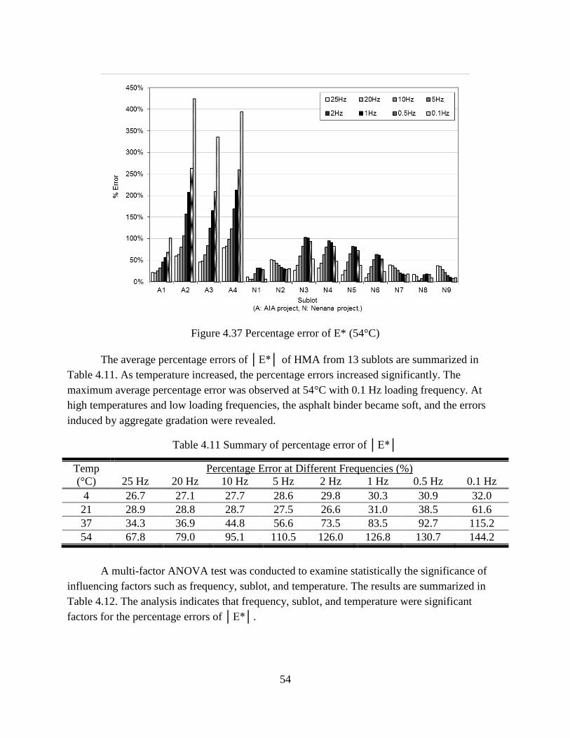
54
Figure 4.37 Percentage error of E* (54°C)
The average percentage errors of │E*│ of HMA from 13 sublots are summarized in
Table 4.11. As temperature increased, the percentage errors increased significantly. The
maximum average percentage error was observed at 54°C with 0.1 Hz loading frequency. At
high temperatures and low loading frequencies, the asphalt binder became soft, and the errors
induced by aggregate gradation were revealed.
Table 4.11 Summary of percentage error of │E*│
Temp
(°C)
Percentage Error at Different Frequencies (%)
25 Hz 20 Hz 10 Hz 5 Hz 2 Hz 1 Hz 0.5 Hz 0.1 Hz
4 26.7 27.1 27.7 28.6 29.8 30.3 30.9 32.0
21 28.9 28.8 28.7 27.5 26.6 31.0 38.5 61.6
37 34.3 36.9 44.8 56.6 73.5 83.5 92.7 115.2
54 67.8 79.0 95.1 110.5 126.0 126.8 130.7 144.2
A multi-factor ANOVA test was conducted to examine statistically the significance of
influencing factors such as frequency, sublot, and temperature. The results are summarized in
Table 4.12. The analysis indicates that frequency, sublot, and temperature were significant
factors for the percentage errors of │E*│.

55
Table 4.12 Multi-factor ANOVA for percentage error of │E*│
Factor Degrees of Freedom P-value Significance
Frequency 7 0.0001031 Significant
Sublot 12 <2.20E-16 Significant
Temperature 3 <2.20E-16 Significant
4.3.2 Flow Test
4.3.2.1 Testing Results
Due to the confining pressure (137 kPa) applied during flow testing, most specimens did
not fail after 10,000 loading cycles; some did not even pass the second zone of deformation.
Therefore, the flow time and flow number values automatically calculated based on the built-in
machine algorithms were meaningless. Lower confining pressure should be used in future testing.
The final test strain was used as an indicator of resistance to permanent deformation.
Figure 4.38 presents the microstrains at the end of the flow time and flow number tests.
The bar chart clearly shows that HMA obtained from the AIA paving project had a substantially
lower microstrain at the end of testing. This result would be mainly due to the greater
compaction effort applied to the AIA HMA. During specimen fabrication, 75 gyrations were
applied to AIA mixtures according to the JMF. Only 20 gyrations were applied to the Nenana
mixtures to reproduce the target air voids specified in the JMF, which was based on the Marshall
mix design method.

56
Figure 4.38 Microstrains at the end of flow tests
4.3.2.2 Analysis of Variance
The variances in microstrains at the end of the flow tests are summarized in Figure 4.39.
Hot mix asphalt obtained from the AIA project not only had lower microstrains, but also had
lower COVs than the Nenana paving project. The HMA of the AIA paving project was designed
by the Superpave mix design method. More compaction efforts were applied on specimens
during the Superpave mix design phase than with the Marshall mix design method. Such high
compaction efforts improve the internal structure of HMA and reduce the variance of
performance induced by the variance of material composition. The variance also changed greatly
along the HMA production indicated by sublot number.
Two-factor ANOVA tests were performed to evaluate the significance of sublot and type
of flow tests on the variance. The results (Table 4.13) show that sublot is a significant factor, but
the type of flow test is not. The procedures of the flow time and flow number tests were similar,
except for a different loading pattern (i.e., static load was used in flow time tests, while dynamic
load was used in flow number tests). The loads used in both tests had the same amplitude (600
kPa). Therefore, the errors included by different types of flow tests were similar.
0
10000
20000
30000
40000
50000
60000
A1 A2 A3 A4 N1 N2 N3 N4 N5 N6 N7 N8 N9
Sublot
(A: AIA project, N: Nenana project,)
Maxim
um
Mic
roS
train
at E
nd o
f T
est .
Flow Time Strain Flow Number Strain

57
Figure 4.39 COV of flow tests
Table 4.13 Two-factor ANOVA for variance of microstrain at end of flow test
Factor Degrees of Freedom P-value Significance
Type of Flow Test 1 0.7460 Not Significant
Sublot 12 0.0002 Significant
4.3.2.3 Analysis of Percentage Error
The percentage errors of microstrain at the end of the flow test are summarized in Figure
4.40. A random pattern was observed on the distribution of percentage error. By performing the
two-factor ANOVA test (Table 4.14), the calculated P-values indicate that percentage error was
not significantly affected by either type of flow test or sublot.
0%
20%
40%
60%
80%
100%
120%
A1 A2 A3 A4 N1 N2 N3 N4 N5 N6 N7 N8 N9
Sublot
(A: AIA project, N: Nenana project,)
Co
eff
icie
nt
of
Vari
ati
on
.
Flow Time Strain Flow Number Strain

58
Figure 4.40 Difference between measured and design value
Table 4.14 Two-factor ANOVA for percentage error of microstrain at end of flow test
Factor Degrees of Freedom P-value Significance
Type of Flow Test 1 0.5561 Not Significant
Sublot 12 0.8329 Not Significant
4.3.3 Creep Stiffness
4.3.3.1 Testing Results
Indirect tensile creep tests were performed on specimens produced from all four scenarios
(L&L, F&F, F&L, and field cores) at three temperatures: -10°C, -20°C, and -30°C. Creep
stiffness was calculated at 50s and 500s at each temperature. The results are summarized in
Figures 4.41 to 4.46. Generally, at all temperatures and testing times, the specimens produced
from F&L scenarios have the highest creep stiffness, and field cores have the lowest stiffness.
Based on the volumetric properties of specimens obtained from four scenarios, field cores always
have the highest VTM, leading to the lowest creep stiffness. However, information obtained
from the study conducted by Marasteanu et al. (2007) shows field cores having higher stiffness
than laboratory-produced specimens, and for laboratory-produced specimens, higher VTM
correlated with higher creep stiffness.

59
As a viscoelastic material, lower stiffness is expected at higher temperatures and longer
loading times. The testing results varied along the sublot numbers, but no trend could be
observed.
Figure 4.41 Creep stiffness at 50s (-10°C)
Figure 4.42 Creep stiffness at 50s (-20°C)
0
2
4
6
8
10
12
A1 A2 A3 A4 N1 N2 N3 N4 N5 N6 N7 N8 N9
Sublot
(A: AIA project, N: Nenana project,)
Cre
ep S
tiffn
ess (
Gpa)
F&L F&F Core
0
5
10
15
20
25
A1 A2 A3 A4 N1 N2 N3 N4 N5 N6 N7 N8 N9
Sublot
(A: AIA project, N: Nenana project,)
Cre
ep S
tiffn
ess (
Gpa)
F&L F&F Core

60
Figure 4.43 Creep stiffness at 50s (-30°C)
Figure 4.44 Creep stiffness at 500s (-10°C)
0
5
10
15
20
25
30
35
A1 A2 A3 A4 N1 N2 N3 N4 N5 N6 N7 N8 N9
Sublot
(A: AIA project, N: Nenana project,)
Cre
ep S
tiffn
ess (
Gpa)
F&L F&F Core
0
1
2
3
4
5
6
A1 A2 A3 A4 N1 N2 N3 N4 N5 N6 N7 N8 N9
Sublot
(A: AIA project, N: Nenana project,)
Cre
ep S
tiffn
ess (
Gpa)
F&L F&F Core

61
Figure 4.45 Creep stiffness at 500s (-20°C)
Figure 4.46 Creep stiffness at 50s (-30°C)
4.3.3.2 Analysis of Variance
Variation analysis was conducted to identify the significance of potential influencing
factors. According to calculation methods provided in AASHTO T322, creep stiffness is
0
2
4
6
8
10
12
14
16
A1 A2 A3 A4 N1 N2 N3 N4 N5 N6 N7 N8 N9
Sublot
(A: AIA project, N: Nenana project,)
Cre
ep S
tiffn
ess (
Gpa)
F&L F&F Core
0
5
10
15
20
25
A1 A2 A3 A4 N1 N2 N3 N4 N5 N6 N7 N8 N9
Sublot
(A: AIA project, N: Nenana project,)
Cre
ep S
tiffn
ess (
Gpa)
F&L F&F Core

62
obtained by stress over mean of strain of three specimens (six sides). Creep can be calculated for
each specimen. Therefore, variance of creep stiffness for HMA obtained in each sublot could be
calculated. The COV of creep stiffness was calculated for three scenarios at each temperature
and loading time. The results are summarized in Figures 4.47 and 4.48. For testing results at 50s,
the maximum variation was obtained on field cores at -30°C with the value of 26%, and
minimum variation was obtained on F&F specimens at -20°C with the value of 10%. The
variance of creep stiffness obtained at 500s is similar to results obtained at 50s. Generally, field
cores possessed the highest variance due to influencing factors encountered during construction,
such as non-homogenous paving and compaction.
A multi-factor ANOVA test was performed to evaluate the significance of influencing
factors. The results (Table 4.15) reveal that the scenario, temperature, or loading time did not
significantly affect the variance of creep stiffness.
Figure 4.47 COV of creep stiffness at 50s
0
5
10
15
20
25
30
-10 -20 -30
Temperature (oC)
CO
V (
%)
F&L F&F Core

63
Figure 4.48 COV of creep stiffness at 50s
Table 4.15 Multi-factor ANOVA for COV of creep stiffness
Factor Degrees of Freedom P-value Significance
Scenario 2 0.2 Not Significant
Temperature 2 0.322 Not Significant
Loading Time 1 0.412 Not Significant
4.3.3.3 Analysis of Percentage Error
Figures 4.49 to 4.54 present the percentage errors of creep stiffness at six different testing
conditions (i.e., three temperatures and two loading periods). Negative errors were observed in
most conditions, indicating generally that specimens made from field-produced HMA possess
lower creep stiffness compared with L&L specimens, especially for the Nenana paving project.
Error varies greatly along sublot and testing scenarios. Multi-factor ANOVA tests were
used to evaluate the significance of factors including sublot, temperature, loading time, and
scenario. The results (Table 4.16) indicate that all of these factors significantly influenced the
percentage error of creep stiffness.
0
5
10
15
20
25
30
-10 -20 -30
Temperature (oC)
CO
V (
%)
F&L F&F Core

64
Figure 4.49 Difference between measured and design value (-10°C, 50s)
Figure 4.50 Difference between measured and design value (-20°C, 50s)

65
Figure 4.51 Difference between measured and design value (-30°C, 50s)
Figure 4.52 Difference between measured and design value (-10°C, 500s)

66
Figure 4.53 Difference between measured and design value (-20°C, 500s)
Figure 4.54 Difference between measured and design value (-30°C, 500s)

67
Table 4.16 Multi-factor ANOVA for % error of creep stiffness
Factor Degrees of Freedom F value Pr(>F) Significance
Sublot 12 29.3 5.41E-12 Significant
Scenario 2 16.4 2.20E-16 Significant
Temperature 2 304.92 2.17E-12 Significant
Loading Time 1 619.62 1.68E-13 Significant
4.3.4 Indirect Tensile Strength
4.3.4.1 Testing Results
After the IDT creep test, the specimens were subjected to vertical load at a constant
crosshead rate of 12.5 mm/min until failure. Indirect tensile strength (ITS) was calculated based
on measured maximum load. The L&L and F&L specimens were tested at -10°C, -20°C, and -
30°C. The F&F specimens were tested at -10°C and -30°C, because only three standard
Superpave specimens (150 mm in diameter and 115 mm in height) were compacted in the field
for each sublot mixture, and each specimen was cut into two IDT specimens. Field cores were
only tested at -20°C, due to the limited number of samples.
Figures 4.55 to 4.57 present the ITS measured at three temperatures. The results from
Figures 4.55 and 4.66 show that the ITS of F&L and F&F is similar, and as the temperature
drops, ITS increases. At -20°C, a comparison of F&L and core results reveals that the ITS of
laboratory-produced specimens is higher than the ITS of field cores. The same observation was
made by Mohammad et al. (2004). However, the study conducted by Marasteanu et al. (2007)
showed that field cores possess higher ITS.

68
Figure 4.55 IDT strength at -10°C
Figure 4.56 IDT strength at -20°C
0
1
2
3
4
5
6
7
A1 A2 A3 A4 N1 N2 N3 N4 N5 N6 N7 N8 N9
Sublot
(A: AIA project, N: Nenana project,)
IDT
Str
ength
(M
pa)
F&L F&F
0
1
2
3
4
5
6
7
8
A1 A2 A3 A4 N1 N2 N3 N4 N5 N6 N7 N8 N9
Sublot
(A: AIA project, N: Nenana project,)
IDT
Str
ength
(M
pa)
F&L Core

69
Figure 4.57 IDT strength at -30°C
4.3.4.2 Analysis of Variance
The COV for each sublot of HMA was calculated based on testing results. These COVs
are summarized in Figures 4.58 to 4.60. Compared with │E*│, microstrains at the end of flow
tests, and creep stiffness, ITS variances were found to be lower. The COVs are in line with the
results from the study performed by Mohammad et al. (2004, 2010). Coefficients of variance
vary with changes of temperature, testing scenario, and sublot. However, particular trends could
not be articulated based on visual examination of graphs. A multi-factor ANOVA test was
performed, and the results (Table 4.17) imply that neither temperature, sublot, nor scenario
significantly affects the variance of ITS.
0
1
2
3
4
5
6
7
8
9
A1 A2 A3 A4 N1 N2 N3 N4 N5 N6 N7 N8 N9
Sublot
(A: AIA project, N: Nenana project,)
IDT
Str
ength
(M
pa)
F&L F&F

70
Figure 4.58 COV of IDT strength
Figure 4.59 COV of IDT strength
0%
2%
4%
6%
8%
10%
12%
14%
16%
18%
20%
A1 A2 A3 A4 N1 N2 N3 N4 N5 N6 N7 N8 N9
Sublot
(A: AIA project, N: Nenana project,)
CO
V
F&L F&F
0%
2%
4%
6%
8%
10%
12%
14%
16%
18%
20%
A1 A2 A3 A4 N1 N2 N3 N4 N5 N6 N7 N8 N9
Sublot
(A: AIA project, N: Nenana project,)
CO
V
F&L Core

71
Figure 4.60 COV of IDT strength
Table 4.17 Multi-factor ANOVA for COV of IDT strength
Factor Degrees of Freedom P-value Significance
Temperature 2 0.6631 Not Significant
Sublot 12 0.4181 Not Significant
Scenario 2 0.6095 Not Significant
4.3.4.3 Analysis of Percentage Error
Error analyses were also conducted for ITS. The percentage errors of IDT strength are
summarized in Figures 4.61 to 4.63. Note that at -10°C and -20°C, specimens obtained from
F&L had higher errors than specimens obtained from the F&F scenario. The errors of field cores
were higher than the errors of specimens of the F&L scenario. To evaluate the effect of sublot,
temperature, and scenario, a multi-factor ANOVA test was performed. The results (Table 4.18)
show that scenario and temperature are significant factors in the percentage errors of IDT
strength, but the effort of sublot was not significant.
0%
5%
10%
15%
20%
25%
30%
A1 A2 A3 A4 N1 N2 N3 N4 N5 N6 N7 N8 N9
Sublot
(A: AIA project, N: Nenana project,)
CO
V
F&L F&F

72
Figure 4.61 Difference between measured and design value (-10°C)
Figure 4.62 Difference between measured and design value (-20°C)

73
Figure 4.63 Difference between measured and design value (-30°C)
Table 4.18 Multi-factor ANOVA for % error of IDT strength
Factor Degrees of Freedom F value Pr(>F) Significance
Sublot 12 0.4925 0.9114 Not Significant
Scenario 2 6.7301 0.0023 Significant
Temperature 2 4.3569 0.0170 Significant
4.4 Correlation
Figure 4.64 summarizes and compares the variability of quality, represented by
coefficient of variation (COV). The COV presented for each quality characteristic is the average
value of all testing results from both projects. The COV of composition properties was found to
be approximately 5%. The COVs of volumetric properties ranged from 2% to 14%.
The COV is calculated as the standard deviation divided by mean value of testing results.
Therefore, with a similar level of standard deviation, a higher COV would be obtained on
variables with small mean values, such as VTM, and a lower COV would be obtained on
variables with greater mean values, such as VFA.
The variances of performance properties are higher than both composition and volumetric
properties. The reason could be that additional errors were introduced during specimen cutting,
sensor installation, and loading, activities not required for composition and volumetric properties.
The sensitivity of performance tests also contributed to the higher variance. Previous studies
have indicated that flow number and flow time have an extremely high level of variation

74
(Bonaquist, 2008). The results from this study confirmed this observation. The flow test results
were represented by the final permanent deformation; the result still exhibited a high COV,
reaching 43%.
a) Composition Properties
b) Volumetric Properties
c) Mechanical Properties
Figure 4.64 Summary of COV by quality characteristic
The purpose of a quality assurance (QA) program is to improve the quality of HMA
mixtures and to make the best effort in ensuring that the performance of installed HMA mixtures
reaches the levels specified in the design. Rather than measuring mechanical properties, which
are considered directly related to pavement performance, composition and/or volumetric
properties are measured in most QA programs. This approach relies on the assumption that
composition and volumetric properties correlate well with mechanical properties; they are
preferred because composition and volumetric properties can be measured easier and faster than
mechanical properties.
Figure 4.65 presents the correlation between composition and mechanical properties
based on data collected from both projects. Generally, correlations between these two types of
properties are less than 0.25, indicating a poor correlation. The percentage passing the #200 sieve
shows the best correlation among the composition properties; however, this value was still less
than 0.4.
Better correlations were observed between volumetric properties and mechanical
properties (Figure 4.66). The mechanical properties of HMA are related to volumetric properties
in nature. The VTM, VMA, and VFA correlate to each other, and the results showed that these
three material properties had a similarly strong relationship with mechanical properties. A strong
correlation between IDT strength and volumetric properties is observed, indicated by correlation
0
1
2
3
4
5
6
7
8
Gradation %AC
Co
eff
icie
nt
of
Vari
ati
on
(%
)
.
0
2
4
6
8
10
12
14
16
VTM VMA VFA
Co
effi
cien
t o
f V
aria
tio
n (
%)
.
0
5
10
15
20
25
30
35
40
45
50
IDT
Strength
Dynamic
Modulus
Creep
Stiffness
Flow Test
Co
eff
icie
nt
of
Vari
ati
on
(%
)
.

75
values over 0.8. The correlation between creep stiffness and dynamic modulus is not as strong as
the correlation between creep stiffness and IDT strength. For QC and QA purposes, volumetric
properties need to be measured, because they delivered more reliable information on material
strength than composition properties.
Figure 4.65 Correlations between composition and mechanical properties
Figure 4.66 Correlation between volumetric and mechanical properties
0
0.05
0.1
0.15
0.2
0.25
0.3
0.35
0.4
0.45
1/2" 3/8" #4 #8 #16 #30 #50 #100 #200 %AC
Co
rrel
atio
n
Creep Stiffness Dynamic Modulus IDT Strength
0
0.1
0.2
0.3
0.4
0.5
0.6
0.7
0.8
0.9
1
%air VMA VFA
Co
rrel
atio
n
Creep Stiffness Dynamic Modulus IDT Strength

76
CHAPTER 5 CONCLUSIONS
Efforts were made to identify the differences in material properties between expected and
as-built hot mix asphalts (HMAs) based on the same job mix formula (JMF). Through fieldwork
and laboratory testing, the variances and errors of HMA quality characteristics during field
production and construction were measured, and the significances of associated influencing
factors were examined using statistical analysis. This chapter presents a summary of research
findings.
Based on testing results and data analyses presented in the previous chapters, the
following conclusions can be drawn:
The measurements of aggregate gradation and binder content obtained from the contractor,
the state highway agency, and third parties are not always consistent with each other.
Variances of composition properties were observed. Generally, the variance of percentage
passing of aggregate at different sieve sizes was less than 2.5%, and the extreme value
reached 4.5%. The variance of binder contents was less than 0.25%. The variance of
aggregate gradation was significantly affected by operator and sublot number. Statistical
analysis indicates that binder content was stable along material production, but data obtained
using the ignition method varied among operators.
Differences were observed in volumetric properties between JMF and specimens prepared
from four scenarios. The differences are significantly affected by sublot and scenario. The
variance of volumetric properties is only affected by testing scenario, that is, L&L, F&L,
F&F, and field cores. The highest STDEVs of VTM, VMA, and VFA were 1.4, 1.2, and 6.7,
respectively.
The COV of mechanical properties was much higher than composition and volumetric
properties. Among all mechanical properties investigated, ITS had the lowest COV at 7%,
and flow tests had the highest COV with values up to 43%.
The │E*│ of field-produced HMA was greatly affected by material production and testing
conditions. The results of multi-factor ANOVA analysis indicate that frequency, sublot, and
temperature are significant factors. The variance of │E*│ is affected by sublot and
temperature.
The permanent deformation at end of each test was used as a measurement of rutting
resistance. A great variance was observed, and COV could reach 100%. The variance is
affected by sublot number.
Generally, creep stiffness obtained from three field scenarios—F&L, F&F, and field cores—
does not agree with the value of L&L specimens. The percentage errors were significantly

77
affected by scenario, sublot, temperature, and loading time. The variance of creep stiffness is
not influenced by these factors.
The results of indirect tensile strength (ITS) tests reveal a difference between field and L&L
scenarios, and the difference changed along the production of HMA. The results of ITS
testing have the lowest variance among all mechanical properties.
Among the three types of property tested, mechanical properties have the greatest sublot-
wise variance. Generally, the observed variance is close to that of previous studies and within
the limits recommended by AASHTO R42.
The correlations between composition and mechanical properties and between volumetric
and mechanical properties were evaluated. Although the volumetric properties provide a
better correlation with mechanical properties than with composition properties, as indicated
by higher R2 values, the correlation was generally found to be weak. Therefore, using
volumetric properties would barely provide reliable estimates of future pavement
performance.

78
REFERENCES
AASHTO T30-08, 2008. “Standard Method of Test for Mechanical Analysis of Extracted
Aggregate.” Washington, DC.
AASHTO T342-11, 2011. “Standard Method of Test for Determining Dynamic Modulus of Hot-
Mix Asphalt Concrete Mixtures.” Washington, DC.
Al-Qadi, I.L., Lahouar, S., and Loulizi, A., 2003. “Successful application of ground-penetrating
radar for quality assurance–quality control of new pavements.” Journal of the
Transportation Research Board, No. 1861, Transportation Research Board of the National
Academies, Washington, DC.
Benson, P.E., 1999. "Quality control/quality assurance implementation for asphalt concrete
specifications in California.” Journal of the Transportation Research Board, No. 1654,
Transportation Research Board of the National Academies Washington, DC.
Biligiri, K.P., Kaloush, K.E., Mamlouk, M.S., and Witczak, M.W. 2007. "Rational Modeling of
Tertiary Flow for Asphalt Mixtures." In Transportation Research Record: Journal of the
Transportation Research Board, No. 2001. Transportation Research Board of the National
Academies, Washington, DC, pp. 63–72.
Bonaquist, R., 2008. “Ruggedness Testing of the Dynamic Modulus and Flow Number Tests
with the Simple Performance Tester.” NCHRP Report 629. Transportation Research Board
of the National Academies, Washington, DC.
Brown, E.R., and Adettiwar, S.M., 1991. “Repeatability and Reproducibility in Hot-Mix Asphalt
and Aggregate Properties.” National Center for Asphalt Technology, Auburn, AL.
Burati, J.L., Weed, R.M., Hughes, C.S., and Hill, H.S., 2003. “Optimal Procedures for Quality
Assurance Specifications.” Clemson University; Federal Highway Administration, p. 347.
Buttlar, W.G., and Harrell, M., 1998. “Development of End-Result and Performance-Related
Specifications for Asphalt Pavement Construction in Illinois.” Crossroads 2000; Ames, IA.
Butts, N. E. and Ksaibati, K. , 2003. “Asphalt Pavement Quality Control/Quality Assurance
Programs in the United States.” Annual Meeting of the Transportation Research Board CD-
room. Transportation Research Board of the National Academies, Washington, DC,
Cominsky, R.J., Killingsworth, B.M., Anderson, R.M., Anderson, D.A., and Crockford, W.W.,
1998. “Quality Control and Acceptance of Superpave-Designed Hot Mix Asphalt.” NCHRP
Report, Issue 409.
Dobrowolski, J., and Bressette, T., 1998. “Development of quality control/quality assurance
specifications by using statistical quality assurance for asphalt concrete pavements in
California.” Journal of the Transportation Research Board, No. 1632, Transportation
Research Board of the National Academies, Washington, DC.

79
Dongré, R., D’Angelo, J., and Copeland, A., 2009. “Refinement of flow number as determined
by asphalt mixture performance tester use in routine quality control–quality assurance
practice.” Journal of the Transportation Research Board, No. 2127, Transportation
Research Board of the National Academies, Washington, DC.
Douglas, K.D., Coplantz, J., Lehmann, R., and Bressette, T., 1999. “Quality control/quality
assurance implementation for asphalt concrete specifications in California.” Journal of the
Transportation Research Board, No. 1654, Transportation Research Board of the National
Academies, Washington, DC.
El-Basyouny, M., and Jeong, M.G., 2010. “Probabilistic performance-related specifications
methodology based on mechanistic–empirical pavement design guide.” Transportation
Research Record: Journal of the Transportation Research Board, No. 2151, Transportation
Research Board of the National Academies, Washington, DC.
Gedafa, D., Hossain, M., Ingram L.S., and Kreider, R., 2011. “Performance related specification
for Superpave pavements in Kansas.” Journal of the Transportation Research Board, No.
2228, Transportation Research Board of the National Academies, Washington, DC.
Hughes, C.S. 2005. “State Construction Quality Assurance Programs”. NCHRP Synthesis of
Highway Practice No. 346. Transportation Research Board, Washington, D.C.,
Hughes, C.S., McGhee, K.K., and Maupin Jr., G.W., 2007. “The Next Step Toward End-Result
Specifications for Hot-Mix Asphalt Materials and Construction.” Virginia Transportation
Research Council; Virginia Department of Transportation; Federal Highway Administration.
Kandhal, P. S. Cooley, L. A., 2003. Accelerated Laboratory Rutting Tests: Evaluation of the
Asphalt Pavement Analyzer. Report 508. National Research Council. Transportation
Research Board. Washington, D.C.
Katicha et al., 2010. Katicha, S. W., Flintsch, G. W., McGhee, K. K, and Loulizi, A. 2010. “Use
of "Mechanistic–Empirical Pavement Design Guide" for Mix Performance Evaluation Using
the Dynamic Modulus: Application to Mix Rutting”, Journal of the Transportation
Research Record, Number: 2180, Transportation Research Board of the National Academies,
Washington, DC.
Von Quintus, H., and Killingsworth, B., 1998. Analysis Relating to Pavement Material
Characterizations and their Effects on Pavement Performance. Brent Rauhut Engineering,
Incorporated; Federal Highway Administration, 223p
Cominsky, R.J., Killingsworth, B.M. Anderson, R.M. Anderson, D.A., and Crockford, W.W.
1998. Quality Control and Acceptance of Superpave-Designed Hot Mix Asphalt, NCHRP
Report 409, Transportation Research Record, National Research Council, Washington, D.C.
Lynn, T., James, R.S., and Wu, P.Y., 2007. “The effect of aggregate degradation on the
volumetric properties of Georgia’s hot mix asphalt.” Journal of the Transportation Research
80
Board, No. 1998, Transportation Research Board of the National Academies, Washington,
DC.
Marasteanu, M., Zofka, A., Turos, M., Li, X., Velasquez, R., Li, X., Buttlar, W., Paulino, G.,
Braham, A., Dave, E., Ojo, J., Bahia, H., Williams, C., Bausano, J., Kvasnak, A., Gallistel,
A., and McGraw, J., 2007. “Investigation of Low Temperature Cracking in Asphalt
Pavements.” Final Report, MN/RC 2007-43, Minnesota Department of Transportation, St.
Paul, MN.
Marasteanu M., Zofka, A., Turos, M., Li, X., Velasquez, R. Li, X., Buttlar, W., Paulino, G.,
Braham, A., Dave, E., Ojo, J., Bahia, H., Williams, C., Bausano, J., Kvasnak, A., Gallistel,
A., and McGraw, J., 2007. Investigation of Low Temperature Cracking in Asphalt
Pavements, Final Report, MN/RC 2007-43, Minnesota Department of Transportation, St.
Paul, Minnesota
Mohammad, L., and Elseifi, M., 2010. “Field Versus Laboratory Volumetrics and Mechanical
Properties.” NCHRP Project 9-48 Phase I Interim Report, Transportation Research Board,
Washington, DC.
Mohammad, L.N., Wu, Z., Zhang, C., Khattak, M.J., and Abadie, C., 2004. “Variability of air
voids and mechanistic properties of plant-produced asphalt mixtures.” Journal of the
Transportation Research Board, No. 1891, Transportation Research Board of the National
Academies, Washington, DC.
Mohammad, L.N., Wu, Z., Myers, L., Cooper, S., and Abadie, C., 2005. “A practical look at the
simple performance tests: Louisiana's experience (with discussion).” Journal of the
Association of Asphalt Paving Technologists: From the Proceedings of the Technical
Sessions, 2005, pp 557–600.
Parker, F. Jr., and Hossain, M.S., 2002. “Statistics for superpave hot-mix asphalt construction
quality control/quality assurance data.” Journal of the Transportation Research Board, No.
1813, Transportation Research Board of the National Academies, Washington, DC.
Patel, A., Thompson, M., Harm, E., and Sheftick, W., 1997. “Developing QC/QA specifications
for hot mix asphalt concrete in Illinois.” Journal of the Transportation Research Board, No.
1575, Transportation Research Board of the National Academies, Washington, DC.
Peterson, P.L., Mahboub, K.C., Anderson, R.H., Masad, E., and Tashman, L., 2003.
“Superpave® laboratory compaction versus field compaction.” Journal of the
Transportation Research Board, No. 1832, Transportation Research Board of the National
Academies, Washington, DC.
Roberts, F.L, Kandhal, P.S., Brown, E.R., Lee, D-Y., and Kennedy, T.W., 1996. Hot Mix
Asphalt Materials, Mixture Design and Construction, 2nd Ed. NAPA Research and
Education Foundation, Lanham, MD.

81
Schmitt, R. L., J. S. Russell, A. S. Hanna, H. U. Bahia, and G. A. Jung. 1998. “Summary of
Current Quality Control/Quality Assurance Practices for Hot-Mix Asphalt Construction.” In
Transportation Research Record 1632, National Research Council, Washington, D.C., pp.
22–31.
Schmitt, R L, Hanna, A.S., Russel, J.S., and Nordhelm, E.V., 2001. “Analysis of bias in HMA
field split-sample testing.” Journal of the Association of Asphalt Paving Technologists, Vol.
70-01.
Smith, G.R., 1998. “NCHRP Synthesis of Highway Practice 263: State DOT Management
Techniques for Materials and Construction Acceptance.” Transportation Research Board,
National Research Council, Washington, DC.
Stroup-Gardiner, M., 2000. "Influence of Segregation on Pavement Performance.” Association
of Asphalt Paving Technologists.
Lynn, T., James, R.S., and Wu P.Y., 2007 “The Effect of Aggregate Degradation on the
Volumetric Properties of Georgia’s Hot Mix Asphalt” Transportation Research Record:
Journal of the Transportation Research Board, Issue 1998, pp 123-131
Transportation Research Board, 2002. “Glossary of Highway Quality Assurance Terms,”
Number E-C037, Transportation Research Board, Committee on Management of Quality
Assurance. National Research Council, Washington, DC.
Transportation Research Board, 2009. “Glossary of Highway Quality Assurance Terms.”
Transportation Research Circular (E-C137), Transportation Research Board of the National
Academies, Washington, DC.
Tsai, B., and Monismith, C.L., 2009. “Quality control–quality assurance sampling strategies for
hot-mix asphalt construction.” Journal of the Transportation Research Board, No. 2098,
Transportation Research Board of the National Academies, Washington, DC.
Turner, P., and West, R.C., 2006. “Evaluation of the effect of sampling location on laboratory-
measured quality control parameters.” Journal of the Transportation Research Board, No.
1946, Transportation Research Board of the National Academies, Washington, DC.
Turochy, R.E., Willis, J.R., and Parker, F., 2006. “Quality assurance of hot-mix asphalt
comparison of contractor quality control and Georgia Department of Transportation data.”
Journal of the Transportation Research Board, No. 1946, Transportation Research Board of
the National Academies, Washington, DC.
Von Quintus, H.L., Scherocman, J.A., Hughes, C.S., and Kennedy, T.W., 1991. “Asphalt-
Aggregate Mixture Analysis System (AAMAS).” NCHRP Report 338, Transportation
Research Board of the National Academies, Washington, DC.

82
Willoughby, K.A., and Mahoney, J.P., 2007. "An Assessment of WSDOT's Hot Mix Asphalt
Quality Control and Assurance Requirements." Washington State Transportation Center;
Washington State Department of Transportation; Federal Highway Administration.

83
Appendix A Summary of Volumetric Properties Results
Scenario ID Air Voids (%) VMA (%) VFA (%)
L&L A 1.2 12.4 90.0
N 3.6 14.6 75.4
F&F
A1 1.6 12.4 87.3
A2 1.6 12.1 87.0
A3 1.8 12.1 85.6
A4 1.8 12.5 85.9
N1 5.3 16.2 67.4
N2 5.2 16.1 67.8
N3 5.1 16.2 68.4
N4 5.9 16.5 64.0
N5 5.3 16.4 67.7
N6 5.5 16.7 66.9
N7 4.7 16.8 71.8
N8 5.4 16.4 67.4
N9 5.8 16.8 65.4
F&L
A1 1.7 12.5 86.8
A2 2.2 12.7 82.6
A3 2.3 12.6 81.8
A4 2.0 12.7 84.4
N1 5.6 16.5 66.0
N2 5.0 16.0 68.5
N3 4.9 16.0 69.3
N4 5.5 16.1 66.0
N5 5.2 16.3 68.1
N6 5.5 16.7 66.9
N7 4.7 16.8 71.8
N8 6.1 17.1 64.4
N9 6.0 17.0 64.6
Core
A1 4.4 15.0 70.9
A2 3.2 13.6 76.4
A3 3.6 13.8 73.7
A4 4.1 14.6 71.8
N1 5.1 16.1 68.0
N2 7.1 17.8 60.2
N3 5.5 16.5 66.8
N4 6.5 17.0 61.9
N5 6.5 17.5 62.7
N6 3.9 15.3 74.3
N7 4.4 16.5 73.6
N8 4.0 15.2 73.8
N9 7.3 18.2 59.7

84
Appendix B Summary of Dynamic Modulus Results
Temp
(oC) Scenario ID
Dynamic Modulus (MPa)
25 Hz 20 Hz 10 Hz 5 Hz 2 Hz 1 Hz 0.5 Hz 0.1 Hz
4oC
L&L A 14042 13963 12263 10533 8388 6927 5529 3174
N 17435 17106 15341 13574 11271 9603 7997 4854
F&L
A1 15738 15604 13662 11785 9451 7847 6299 3721
A2 17854 17253 15166 13189 10686 8912 7259 4240
A3 17482 17285 14650 12552 10119 8419 6874 4032
A4 13308 13214 11621 10042 8111 6798 5585 3430
N1 11741 11353 10013 8726 7135 6042 5018 3054
N2 8960 8559 7360 6229 4872 3963 3166 1741
N3 11947 11647 10461 9300 7844 6816 5858 3869
N4 12703 12257 10916 9612 7981 6846 5793 3720
N5 12292 11897 10636 9418 7856 6767 5749 3760
N6 12099 11747 10330 9087 7537 6502 5492 3488
N7 15197 14607 12570 10618 8298 6708 5384 2917
N8 12414 12050 10489 9044 7282 6062 4948 2908
N9 10972 10586 9213 7900 6255 5115 4084 2221
21
L&L A 3704 3405 2537 1851 1182 829 585 265
N 5661 5286 4059 2968 1847 1239 826 347
F&L
A1 3865 3535 2642 1945 1274 921 676 348
A2 3918 3571 2703 2039 1421 1116 907 629
A3 4278 3915 2949 2201 1499 1149 908 592
A4 5113 4734 3685 2828 1975 1513 1185 730
N1 3608 3370 2628 2008 1361 999 728 344
N2 2131 1947 1432 1035 652 459 325 155
N3 4394 4177 3401 2727 1981 1535 1178 601
N4 4323 4045 3218 2517 1768 1331 993 487
N5 4328 4085 3296 2625 1889 1453 1104 556
N6 4107 3869 3093 2434 1722 1308 982 478
N7 3352 3080 2284 1664 1066 752 533 248
N8 4021 3748 2883 2173 1451 1052 760 356
N9 3018 2776 2061 1501 958 678 483 230

85
Temp
(oC) Scenario ID
Dynamic Modulus (MPa)
25 Hz 20 Hz 10 Hz 5 Hz 2 Hz 1 Hz 0.5 Hz 0.1 Hz
37
L&L A 765 679 472 327 200 146 110 62
N 1006 848 542 349 204 150 115 77
F&L
A1 929 816 592 433 292 228 185 125
A2 1223 1109 852 675 516 449 399 324
A3 1112 1008 767 599 449 386 339 270
A4 1367 1237 939 729 539 456 395 305
N1 897 799 578 414 268 197 148 82
N2 499 435 308 217 137 104 82 53
N3 1273 1167 869 637 413 303 224 118
N4 1335 1211 879 629 397 286 210 114
N5 1174 1072 792 576 370 270 200 107
N6 1104 1004 733 528 333 242 178 95
N7 618 528 369 258 161 123 97 62
N8 834 740 530 375 237 176 136 84
N9 631 547 388 275 174 134 106 69
54
L&L A 195 172 126 92 61 51 43 31
N 192 159 108 77 52 46 41 32
F&L
A1 222 196 144 106 71 59 50 37
A2 475 429 357 305 252 235 220 194
A3 419 382 312 261 208 192 177 153
A4 498 448 367 310 251 232 214 186
N1 301 285 211 153 98 76 63 42
N2 185 168 126 95 64 54 54 44
N3 353 319 232 167 109 88 72 49
N4 354 349 269 202 136 106 88 60
N5 308 270 193 138 92 74 62 43
N6 327 302 224 164 109 86 70 47
N7 284 245 180 135 94 83 73 58
N8 275 242 176 132 91 77 66 50
N9 197 171 124 92 65 56 49 39
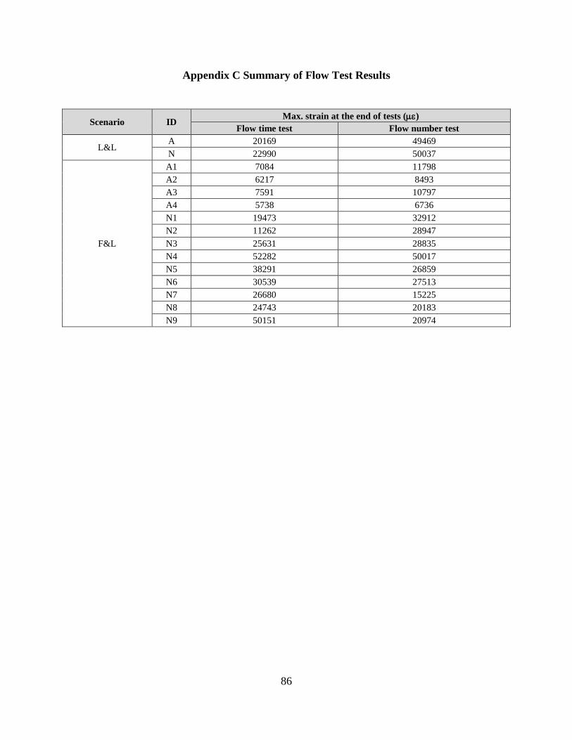
86
Appendix C Summary of Flow Test Results
Scenario ID Max. strain at the end of tests ()
Flow time test Flow number test
L&L A 20169 49469
N 22990 50037
F&L
A1 7084 11798
A2 6217 8493
A3 7591 10797
A4 5738 6736
N1 19473 32912
N2 11262 28947
N3 25631 28835
N4 52282 50017
N5 38291 26859
N6 30539 27513
N7 26680 15225
N8 24743 20183
N9 50151 20974

87
Appendix D Summary of IDT Creep Test Results
Scenario ID
Creep Stiffness (GPa)
50s loading 500s loading
-10 oC -20 oC -30 oC -10 oC -20 oC -30 oC
L&L 6.16 17.54 20.00 2.81 10.15 14.08
9.82 21.20 27.46 7.03 16.43 23.83
F&L
A1 6.89 14.76 21.43 3.57 8.03 17.21
A2 8.68 15.14 25.99 4.18 8.30 19.97
A3 8.83 14.28 23.42 4.33 8.45 19.33
A4 8.70 20.21 25.01 4.84 13.81 19.56
N1 6.23 20.33 15.98 2.96 12.75 11.81
N2 10.31 15.65 23.39 4.96 10.10 19.29
N3 6.64 16.68 19.11 2.97 10.20 15.86
N4 4.75 17.66 23.13 1.88 11.13 19.22
N5 6.72 16.95 18.96 3.51 10.95 15.30
N6 8.23 16.68 20.13 3.49 9.47 15.03
N7 5.60 10.61 29.19 2.18 5.47 20.93
N8 5.20 12.67 21.63 2.17 7.34 17.27
N9 6.69 12.77 15.94 2.87 7.66 12.20
F&F
A1 5.97 14.62 22.57 2.47 8.65 17.17
A2 4.42 16.95 20.94 1.84 10.59 17.16
A3 5.19 13.64 18.35 2.11 8.51 14.88
A4 6.98 12.75 24.83 3.04 7.68 18.89
N1 5.69 13.75 20.34 2.32 8.11 14.54
N2 5.35 14.83 21.98 2.17 8.12 15.27
N3 4.66 13.81 16.56 1.97 8.43 12.77
N4 4.78 14.69 13.63 1.89 9.20 10.06
N5 4.61 13.93 21.31 1.85 7.53 15.79
N6 3.82 11.97 11.48 1.48 6.39 5.84
N7 5.61 11.95 15.85 2.34 5.77 7.89
N8 5.85 13.46 17.06 2.42 6.81 11.73
N9 5.72 12.58 18.82 2.36 5.94 13.88
Core
A1 5.17 10.19 25.04 1.87 4.82 16.32
A2 6.81 13.28 22.34 2.49 6.51 16.56
A3 5.10 11.68 14.12 2.05 6.23 12.08
A4 3.99 12.30 13.14 1.50 6.75 9.80
N1 5.28 10.66 17.48 1.89 5.69 13.75
N2 2.87 9.93 18.21 1.02 5.03 13.78
N3 2.40 13.80 21.67 0.89 6.05 16.92
N4 4.01 11.29 15.29 1.43 5.93 12.32
N5 3.91 10.09 12.51 1.48 5.30 10.62
N6 3.33 11.70 11.80 1.17 5.91 9.88
N7 2.68 7.43 14.38 0.90 3.55 11.90
N8 4.69 12.65 15.14 1.67 6.40 11.84
N9 3.07 9.05 13.23 1.08 4.86 9.70

88
Appendix E Summary of Flow Test Results
ID
-10oC -20oC -30oC
Scenario IDT Strength
(MPa) Scenario
IDT Strength
(MPa) Scenario
IDT Strength
(MPa)
AIA L&L 6.8 L&L 6.9 L&L 7.1
N L&L 3.8 L&L 4.7 L&L 5.1
A1 F&F 5.7 F&L 7.5 F&F 6.7
A2 F&F 5.9 F&L 7.5 F&F 7.9
A3 F&F 5.7 F&L 7.0 F&F 6.7
A4 F&F 6.1 F&L 6.4 F&F 8.2
N1 F&F 4.0 F&L 5.3 F&F 5.5
N2 F&F 4.5 F&L 4.7 F&F 5.4
N3 F&F 3.6 F&L 5.6 F&F 5.1
N4 F&F 4.1 F&L 5.2 F&F 5.1
N5 F&F 4.0 F&L 5.0 F&F 5.1
N6 F&F 4.1 F&L 4.6 F&F 5.6
N7 F&F 3.9 F&L 5.7 F&F 4.9
N8 F&F 4.7 F&L 4.5 F&F 5.6
N9 F&F 3.8 F&L 5.1 F&F 5.4
A1 F&L 4.9 Core 5.1 F&L 8.0
A2 F&L 5.4 Core 6.6 F&L 7.5
A3 F&L 5.5 Core 5.5 F&L 7.3
A4 F&L 5.7 Core 5.5 F&L 6.5
N1 F&L 4.7 Core 4.5 F&L 6.2
N2 F&L 4.1 Core 3.4 F&L 5.5
N3 F&L 4.8 Core 4.3 F&L 5.9
N4 F&L 4.1 Core 3.7 F&L 6.1
N5 F&L 4.3 Core 3.8 F&L 6.1
N6 F&L 4.1 Core 4.4 F&L 5.2
N7 F&L 4.4 Core 4.0 F&L 4.9
N8 F&L 4.0 Core 4.0 F&L 4.0
N9 F&L 4.3 Core 3.0 F&L 5.5