Verification Methods for Dense and Sparse

Systems of Equations ∗

S.M. Rump, Hamburg

In this paper we describe verification methods for dense and large sparse systems of

linear and nonlinear equations. Most of the methods described have been developed by

the author. Other methods are mentioned, but it is not intended to give an overview over

existing methods.

Many of the results are published in similar form in research papers or books. In

this monograph we want to give a concise and compact treatment of some fundamental

concepts of the subject. Moreover, many new results are included not being published

elsewhere. Among them are the following.

A new test for regularity of an interval matrix is given. It is shown that it is significantly

better for classes of matrices.

Inclusion theorems are formulated for continuous functions not necessarily being differ-

entiable. Some extension of a nonlinear function w.r.t. a point x is used which may be a

slope, Jacobian or other.

More narrow inclusions and a wider range of applicability (significantly wider input

tolerances) are achieved by (i) using slopes rather than Jacobians, (ii) improvement of

slopes for transcendental functions, (iii) a two-step approach proving existence in a small

and uniqueness in a large interval thus allowing for proving uniqueness in much wider

domains and significantly improving the speed, (iv) use of an Einzelschrittverfahren, (v)

computing an inclusion of the difference w.r.t. an approximate solution.

Methods for problems with parameter dependent input intervals are given yielding inner

and outer inclusions.

An improvement of the quality of inner inclusions is described.

Methods for parametrized sparse nonlinear systems are given for expansion matrix being

(i) M-matrix, (ii) symmetric positive definite, (iii) symmetric, (iv) general.

A fast interval library having been developed at the author’s institute is presented being

significantly faster compared to existing libraries.

∗in J. Herzberger, editor, Topics in Validated Computations — Studies in Computational Mathematics,pages 63-136, Elsevier, Amsterdam, 1994

1

2

A common principle of all presented algorithms is the combination of floating point

and interval algorithms. Using this synergism yields powerful algorithms with automatic

result verification.

3

Contents

0 Introduction 4

0.1 Notation . . . . . . . . . . . . . . . . . . . . . . . . . . . . . . . . . . . . . 6

1 Basic results 7

1.1 Some basic lemmata . . . . . . . . . . . . . . . . . . . . . . . . . . . . . . 8

1.2 Regularity of interval matrices . . . . . . . . . . . . . . . . . . . . . . . . . 13

2 Dense systems of nonlinear equations 16

2.1 An existence test . . . . . . . . . . . . . . . . . . . . . . . . . . . . . . . . 16

2.2 Refinement of the solution . . . . . . . . . . . . . . . . . . . . . . . . . . . 21

2.3 Verification of uniqueness . . . . . . . . . . . . . . . . . . . . . . . . . . . . 22

2.4 Verification of existence and uniqueness for large inclusion intervals . . . . 22

2.5 Inner inclusions of the solution set . . . . . . . . . . . . . . . . . . . . . . . 25

2.6 Sensitivity analysis with verified inclusion of the sensitivity . . . . . . . . . 30

3 Expansion of functions and slopes 32

4 Dense systems of linear equations 36

4.1 Optimality of the inclusion formulas . . . . . . . . . . . . . . . . . . . . . . 38

4.2 Inner inclusions and sensitivity analysis . . . . . . . . . . . . . . . . . . . . 40

4.3 Data dependencies in the input data . . . . . . . . . . . . . . . . . . . . . 45

5 Special nonlinear systems 50

6 Sparse systems of nonlinear equations 53

6.1 M -matrices . . . . . . . . . . . . . . . . . . . . . . . . . . . . . . . . . . . 54

6.2 Symmetric positive definite matrices . . . . . . . . . . . . . . . . . . . . . 58

6.3 General matrices . . . . . . . . . . . . . . . . . . . . . . . . . . . . . . . . 63

7 Implementation issues: An interval library 65

8 Conclusion 69

4

0. Introduction

Verification methods, inclusion or self-validating methods deliver bounds for the solu-

tion of a problem which are verified to be correct. Such verification includes all conversion,

rounding or other procedural errors. This is to be sharply distinguished from any heuristic

such as, for example, computing in different precisions and using coinciding figures. Such

techniques may fail. Consider the following example [77].

f := 333.75 b6 + a2(11 a2b2 − b6 − 121 b4 − 2) + 5.5 b8 + a/(2 b)

with a = 77617.0 and b = 33096.0

Even if the powers are executed by successive multiplications in order to avoid transcen-

dental function calls, then on an IBM S/370 computing in single (∼ 7 decimals), double

(∼ 16 decimals) and extended (∼ 33 decimals) precision we obtain the following results

single precision f = 1.17260361 . . .

double precision f = 1.17260394005317847 . . .

extended precision f = 1.17260394005317863185 . . .

where the coinciding figures are underlined. This might lead to the conclusion that f =

+ 1.1726 seems at least to be a reasonably good approximation for f . The true value is

f = − 0.827396 . . .

Floating point algorithms usually deliver good approximations for the solution of a given

problem. However, those results are not verified to be correct and may be afflicted with a

smaller or larger error. As an example, consider the determination of the eigenvalues of

the following matrix A.

A =

1 −1 −1

1 1 −1 0. . . . . .

......

1 1 −1 0

1 0 0

1 2

∈ Mnn(IR) (1)

Applying [V, D] = eig(A) from MATLAB [57] which implements EISPACK algorithms

[87] delivers the matrix of eigenvectors V and the diagonal matrix D of eigenvalues. The

eigenvalues for n = 17 are plotted in the complex plane.

5

0.85 0.9 0.95 1 1.05 1.1 1.15-0.15

-0.1

-0.05

0

0.05

0.1

0.15

No warning is displayed or could be found in the documentation. Checking the residual

yields

norm (A ∗ V − V ∗D) = 2.6 · 10−14.

Therefore the user might expect to have results of reasonable accuracy. However, checking

the rank of V would give rank (V ) = 1, and indeed

A = X−1 ·

11 1

. . . . . .

1 1

·X with X =

1 11 1

. . ....1

, X−1 =

1 −11 −1

. . ....1

.

That means, A from (1) has exactly one eigenvalue equal to 1.0 of multiplicity n. Such

errors are rare, but to cite Kahan [44]:

Kahan: “Significant discrepancies [between the computed and the true result]

are very rare, too rare to worry about all the time, yet not rare enough to

ignore.”

Verification algorithms aim to fill this gap by always producing correct results. One

basic tool of verification algorithms is interval analysis. The most basic, principle property

of interval analysis is the isotonicity. This means that for interval quantities [A], [B] in

proper interval spaces

∀ a ∈ [A] ∀ b ∈ [B] : a ∗ b ∈ [A] ∗ [B] (2)

6

for any suitable operation ∗ (cf. [61], [8], [66]). This leads to the remarkable property

that the range of a function f over a box can be rigorously estimated by replacing real

operations by their corresponding interval operations during the evaluation of f . This is

possible without any further knowledge of f , such as Lipschitz conditions. On the other

hand, one also quickly observes that overestimation may occur due to data dependencies.

The main goal of verification algorithms is to make use of this remarkable range esti-

mation and to avoid overestimation where possible. In general, this implies use of floating

point arithmetic as much as possible and restriction of interval operations to those specific

parts where they are really necessary. This is very much in the spirit of Wilkinson [90],

who wrote in 1971:

Wilkinson: “In general it is the best in algebraic computations to leave

the use of interval arithmetic as late as possible so that it effectively

becomes an a posteriori weapon.”

(3)

0.1. Notation

In this paper all operations are power set operations except when explicitly stated

otherwise. For example (ρ denotes the spectral radius of a matrix), a condition like

Z ∈ IPIRn, C ∈ IPMnn(IR), X ∈ IPIRn closed and bounded with

Z + C ·X ⊆ int(X) ⇒ ∀ C ∈ C : ρ(C) < 1(4)

is to read

{ z + C · x | z ∈ Z, C ∈ C, x ∈ X } ⊆ int(X).

Theoretical results are mostly formulated using power sets and power set operations.

In a practical implementation we mostly use [Z] ∈ IIIRn, [C] ∈ IIMnn(IR), [X] ∈ IIIRn.

Then (4) can be used to verify ρ(C) < 1 for all C ∈ [C] on the computer by using the

fundamental principle of interval analysis, the isotonicity (0.2). Denote interval operations

by 3∗ , ∗ ∈ {+,−, ·, /}. Then

[Z] 3+ [C] 3· [X] ⊆ int(X) ⇒[Z] + [C] · [X] ⊆ [Z] 3+ [C] 3· [X] ⊆ int(X),

where the operations in the first part of the second line are power set operations as in (4)

using the canonical embeddings IIIRn ⊆ IPIRn, IIMnn(IR) ⊆ IPMnn(IR). For f : IRn → IRn,

X ∈ IPIRn we define f(X) := { f(x) | x ∈ X } ∈ IPIRn. For more details see standard

text books on interval analysis, among them [7], [8], [11], [66], [31], [61], [70]. We also use

interval rounding 3 from the power set IPS over S to the set of intervals IIS over S for all

suitable S:

X ∈ IPS ⇒ 3(X) ∈ IIS with 3 (X) :=⋂{ [Y ] ∈ IIS | X ⊆ [Y ] }.

7

3(X) is also called the interval hull of X.

With one exception, in all of the presented theorems given in this paper it is always

possible to replace the power set operations by the corresponding interval operations with-

out sacrificing the validity of the assertions. The exception is so-called inner inclusions.

They allow a sensitivity analysis of parametrized nonlinear systems w.r.t. finite changes

in the parameters. This exception is stated explicitly. We prefer using power set opera-

tions, because they simplify the proofs, and allow use of the usual symbols for arithmetic

operations.

Interval quantities are written in brackets, for example an interval vector [X] ∈ IIIRn

with components [X]i ∈ IIIR or simply Xi. The lower and upper bounds are denoted by

inf([X]) ∈ IRn and sup([X]) ∈ IRn, where sometimes we also use the notation [X] = [X,X]

with X, X ∈ IRn. Absolute value | · |, comparison ≤, midpoint mid([X]), width w([X])

and so forth are always to be understood componentwise. int([X]) denotes the topological

interior, I is the identity matrix of proper dimension and

[X], [Y ] ∈ IIIRn : [X] $ [Y ] ⇔ [X] ⊆ [Y ] and [X]i 6= [Y ]i for i = 1 . . . n.

Most of the following results are given for intervals over real numbers. We want to stress

that all results remain true over the domain of complex numbers.

1. Basic results

Let f : D ⊆ IRn → IRn be a continuous mapping. Consider the function g : D ⊆ IRn →IRn defined by

g(x) := x−R · f(x) (5)

for x ∈ D and some fixed matrix R ∈ Mnn(IR). Then g is also continuous, and for convex

and compact ∅ 6= X ⊆ D

g(X) ⊆ X implies the existence of some x ∈ X : g(x) = x

by Brouwer’s Fixed Point Theorem [33]. If, moreover,

R is regular, then f(x) = 0.

That means, if we can find a suitable set X ⊆ D and could prove that g maps X into

itself and that R is regular, then X is verified to contain a zero of f . Therefore, in the

following we will first concentrate

– on verification procedures for g(X) ⊆ X and

– on verification of the regularity of R.

Many of the following considerations hold for general closed and bounded and possibly

convex sets. Also, many proofs become simpler when using power set operations, whereas

8

the specialization to interval operations is almost always straightforward by replacing the

power set operations by the corresponding interval operations and using the basic principle

of isotonicity (2). Therefore, we give the results in a more general setting in order not to

preclude specific interval representations such as, for example, circular arithmetic.

g(X) ⊆ X cannot be verified by testing

X −R · f(X) = { x1 −R · f(x2) | x1, x2 ∈ X } ⊆ X

unless R · f(X) ≡ 0. Therefore we need some expansion of f . For this chapter, we make

the following, general assumption:

Let f : D ⊆ IRn → IRn be continuous, sf : D ×D → Mnn(IR) such that

x ∈ D, x ∈ D ⇒ f(x) = f(x) + sf (x, x) · (x− x).(6)

Such expansion functions sf can be computed efficiently by means of slope functions or,

if f is differentiable, by automatic differentiation techniques. In Chapter 3 we will discuss

such techniques in detail; for the moment we assume that such an sf satisfying (6) is

given.

1.1. Some basic lemmata

It turns out to be superior not to include a zero x of a function itself but the difference

w.r.t. some approximate solution x. Note that here and in the following there are no

preassumptions on the quality of x. Therefore, we immediately go for inclusions of x− x.

For given nonempty, compact and convex X ⊆ D define Y := X − x ⊆ IRn. We do not

assume x ∈ X. Then with g from (5)

x ∈ X ⇒ g(x)− x = x− x−R · f(x)

= −R · f(x) + {I −R · sf (x, x)} · (x− x)

∈ −R · f(x) + {I −R · sf (x, x + Y )} · Y.

With the abbreviations

z := −R · f(x) ∈ IRn and C := I −R · sf (x, x + Y ) ∈ IPMnn(IR) (7)

this means

z + C · Y ⊆ Y ⇒ g(X)− x ⊆ Y ⇒ g(X) ⊆ X. (8)

In other words, z+C ·Y ⊆ Y is a sufficient condition for g(X) ⊆ X, and our first problem

is solved.

For the second problem, the verification of the regularity of R, we give a characterization

of the convergence of the iteration matrices C in (8). The following lemma has been given

9

in [74].

Lemma 1.1. Let Z ∈ IPIRn, C ∈ IPMnn(IR) and let some closed and bounded

∅ 6= X ∈ IPIRn be given. Then

Z + C ·X ⊆ int(X) (9)

implies for every C ∈ C : ρ(C) < 1.

Proof. Let z ∈ Z, C ∈ C fixed but arbitrary. Then (9) implies z + C ·X ⊆ int(X).

Abbreviating Y := (X + iX)− (X + iX) implies

C · Y = {C · (x1 + i x2)− C · (x3 + i x4) | xν ∈ X for 1 ≤ ν ≤ 4 }= z + C ·X + i · (z + C ·X)− (z + C ·X)− i · (z + C ·X)

⊆ int(Y ).

(10)

Suppose C 6= (0) and let λ ∈ C, 0 6= x ∈ Cn be an eigenvalue/eigenvector pair of C.

Define

Γ ∈ IPC by Γ := { γ ∈ C | γ · x ∈ Y }. (11)

Then by the definition of Y we have 0 ∈ Y and therefore Γ 6= ∅. Moreover, Y is closed

and bounded, hence Γ has this property and there is some γ∗ ∈ Γ with

|γ∗| = maxγ∈Γ

|γ|.

(11) implies γ∗ x ∈ Y and (10) yields C · (γ∗x) = (γ∗λ) · x ∈ int(Y ), and by the definition

of γ∗ and Γ, |γ∗λ| < |γ∗|. Therefore |λ| < 1, and since C ∈ C was chosen arbitrarily the

lemma is proved.

In a practical implementation we use interval quantities and interval operations. Inter-

estingly enough, if the set X in Lemma 1.1 is replaced by an interval vector, then we can

sharpen the result under weaker assumptions. We start with the following lemma which

can be found in [76]. The presented proof has been given by Heindl [32].

Lemma 1.2. Let Z ∈ IPIRn, C ∈ IPMnn(IR) and [X] ∈ IIIRn be given. Then

3(Z + C · [X]) $ [X] (12)

implies ρ(C) < 1 for every C ∈ C.

Proof. Let z ∈ Z, C ∈ C fixed but arbitrary and let [Y ] := 3(z + C · [X]) ∈ IIIRn.

Then [Y ] $ [X], which means componentwise inclusion but inequality. Thus there is an

10

ε-perturbation z∗ of z with 3(z∗ + C · [X]) ⊆ int([X]). Lemma 1.1 finishes the proof.

If inequality is only required for some components of (12), then C ∈ C must be

irreducible to prove ρ(C) < 1. Next, we weaken the assumptions even more by in-

troducing an Einzelschrittverfahren and a dependency of the iteration matrices C on

the set [X]. Let C : IRn → Mnn(IR) be a mapping. Then for [X] ∈ IIIRn the set

C [X] := C([X]) = {C(x) | x ∈ [X] } is well-defined. We define the following procedure

to replace (12):

for i = 1 . . . n do

[U ] := [Y1, . . . , Yi−1, Xi, . . . , Xn];

Yi := {3(Z + C [U ] · [U ])}i

(13)

Here the Yi ∈ IIIR and [U ] is defined by its components Yν , Xµ, the ν-th, µ-th component

of Y , X, respectively. Obviously, Y is computed using an Einzelschrittverfahren, where

the iteration vector [U ] as well as the set of iteration matrices C [U ] changes in every step.

With these preperations we can state the following lemma.

Lemma 1.3. Let Z ∈ IPIRn, C : IRn → Mnn(IR) be a mapping and, for S ∈ IPIRn, set

CS := C(S) = {C(s) | s ∈ S }. Let [X] ∈ IIIRn and define [Y ] ∈ IIIRn by (13). If

[Y ] $ [X], (14)

then for every C ∈ C [Y ] ρ(|C|) < 1 holds.

Proof. In every step of (13), [U ] satisfies [Y ] ⊆ [U ] because of (14). For fixed but

arbitrary z ∈ Z, C ∈ C [Y ] we have

∀ 1 ≤ i ≤ n : [U ] := [Y1, . . . , Yi−1, Xi, . . . , Xn] ⇒ {3(z + C · [U ])}i ⊆ Yi $ Xi.

Thus

w({3(z + C · [U ])}i) = w({3(C · [U ])}i) = {|C| · w([U ])}i ≤ {w([Y ])}i < {w([X])}i

using some basic facts of interval analysis (see [8]). Thus abbreviating x := w([X]) ∈ IRn,

y := w([Y ]) ∈ IRn we have 0 ≤ y < x and

∀ 1 ≤ i ≤ n : {|C| · (y1, . . . , yi−1, xi, . . . , xn)T}i ≤ yi < xi. (15)

For 0 < εi ∈ IR, 1 ≤ i ≤ n define

y∗i :={|C| · (y∗1, . . . , y∗i−1, xi, . . . , xn)T

}i+ εi.

For sufficiently small εi we still have y∗i < xi. Hence for 1 ≤ i ≤ n

{|C| · y∗}i ≤{|C| · (y∗1, . . . , y∗i−1, xi, . . . xn)T

}i= y∗i − εi < y∗i

11

or |C| · y∗ < y∗. Thus a theorem by Collatz [17] implies ρ(|C|) < 1.

A lemma similar to the preceeding one has been given in [76]. The stronger assertion

that even the absolute value of the iteration matrix is contracting is due to the symmetry

of interval vectors in every component individually w.r.t. their midpoint. There are a

number of other conditions proving the contractivity of a matrix, see for example [76].

In an application of Lemma 1.1 or 1.3, we need a set X to check the contractivity

conditions. If we restrict our attention, for a moment, to the point case Z = z ∈ IRn,

C = C ∈ Mnn(IR), then ρ(C) < 1 implies invertibility of I − C, and this yields

x := (I − C)−1z ⇒ z + C · x = x.

This fixed point is unique, and a fortiori it follows that x ∈ X. In other words the set

X must contain the fixed point of the mapping z + C · x (in our applications, this fixed

point will be the zero of the function f). But rather than testing a number of sets X

potentially containing a fixed point, we would like to construct such a set, for example by

means of an iteration. We could define

Xk+1 := z + C ·Xk for some X0. (16)

However, x 6∈ X0 immediately implies x 6∈ X1 and therefore x 6∈ Xk for all k ∈ IN. But

even if x ∈ X0, simple examples show that Xk+1 ⊆ Xk need not be satisfied for any k ∈ IN

using iteration (16). If [X0] is an interval vector and ρ(|C|) < 1, then truly w([X]) → 0.

However, we need [Xk+1] ⊆ [Xk]. Consider

z = 0, C =

0 0.5

0.5 0

, [X0] =

[−10, 10]

[−1, 1]

.

Obviously ρ(|C|) < 1. Since [X0] = −[X0], we only need to compute the sequence

x0 := |[X0]|, xk+1 := |C| · xk and to check xk+1 < xk. We have

x0 =

10

1

, x1 =

0.5

5

, x2 =

2.5

0.25

, x3 =

0.125

1.25

, . . .

and obviously xk+1 < xk never occurs for any k ∈ IN.

In an application for systems of nonlinear equations, the problem is even more involved,

since the iteration matrix C is no longer constant. If we assume C to be constant, we

can give a complete overview of the convergence behaviour of the corresponding affine

iteration for the case of power set operations as well as for the case of interval operations,

if we use the so-called ε-inflation introduced in [74]. Below we give corresponding theorems

12

from [76] and [81], which are stated without proof. Interval iterations with ε-inflation for

nonconstant iteration matrix have been investigated by Mayer [59].

Theorem 1.4. Let S ∈ {IR, C} and C ∈ Mnn(S) be an arbitrary matrix, ∅ 6= Z ∈ IPSn

and ∅ 6= X0 ∈ IPSn be bounded sets of vectors, and define

Xk+1 := Z + C ·Xk + Uεk(0) for k ∈ IN,

where Uεk+1⊆ Uεk

and U ⊆ Uεkare bounded for every k ∈ IN, for some ∅ 6= U ∈ IPSn

with 0 ∈ int(U). Then the following two conditions are equivalent:

i) ∀ ∅ 6= X0 ∈ IPSn bounded ∃ k ∈ IN : Z + C ·Xk ⊆ int(Xk)

ii) ρ(C) < 1.

The operations in the above theorem are the power set operations. A similar theorem

does not necessarily hold for sets of matrices C. The condition Z + C · X ⊆ int(X)

immediately implies ρ(C1 · C2) < 1 for all C1, C2 ∈ C. However, there are examples of

convex sets of matrices C with ρ(C) < 1 for all C ∈ C, but ∃ C1, C2 ∈ C : ρ(C1 ·C2) > 1

(see [76]).

In case of interval operations we can prove a similar theorem for interval matrices. The

proof in the real case is given in [76], a slightly more general form of the complex case

is proved in [81]. In conjunction with Lemma 1.3 this offers a possibility to verify the

regularity of a matrix or a set of matrices. We will need this later.

Theorem 1.5. Let S ∈ {IR, C} and let [C] ∈ IIMnn(S), [Z] ∈ IISn and for [X0] ∈ IISn

define the iteration

[Xk+1] := [Z] 3+ [C] 3· [Xk] 3+ [Ek] for k ∈ IN

where [Ek] ∈ IISn, [Ek] → [E] ∈ IISn with 0 ∈ int([E]) and all operations are interval

operations. Then the following two conditions are equivalent:

i) ∀ [X0] ∈ IISn ∃ k ∈ IN : [Z] 3+ [C] 3· [Xk] ⊆ int([Xk])

ii) ρ(|[C]|) < 1.

The absolute value of a complex interval matrix is defined as the sum of absolute

values of the real and imaginary part. In practical applications, it may be superior to

go from intervals to an absolute value iteration. If |Z| denotes the supremum of |z| for

z ∈ Z ∈ IPIRn and |C| is defined similarly for C ∈ IPMnn(IR), then we can state a

straightforward application of Lemma 1.3.

Lemma 1.6. Let Z ∈ IPIRn, C : IRn → Mnn(IR) be a mapping, and for S ∈ IPIRn let

CS := C(S) = {C(s) | s ∈ S }. Let 0 < x ∈ IRn and define y ∈ IRn for 1 ≤ i ≤ n by

yi := {|Z|+ |C [U ]| · u}i with u := (y1, . . . , yi−1, xi, . . . , xn)T and [U ] := [−u, +u].

13

If

y < x

then for every C ∈ C [−y,+y] holds ρ(|C|) < 1.

In a practical implementation the verification of the assumptions of Lemma 1.6 needs

only rounding upwards. Therefore no switching of the rounding mode is necessary. More-

over, only the upper bounds of the interval quantities need to be stored, which is advan-

tageous, especially for large matrices. This gains much more than the factor 2 that might

be expected. We will come to this in more detail in Chapter 7.

1.2. Regularity of interval matrices

The preceeding Theorem 1.5 and Lemma 1.6 can be used for the computational verifica-

tion of the regularity of an interval matrix. An interval matrix [A] is called regular if every

A ∈ [A] is regular, whereas an interval matrix is called strongly regular if mid([A])−13· [A]

is regular.

Theorem 1.7. Let [A] ∈ IIMnn(IR) be given, R ∈ Mnn(IR) and 0 < x ∈ IRn. Let

C ∈ Mnn(IR) with C := |I −R · [A]| and define x(k), y(k) ∈ IRn for k ≥ 0 by

y(k)i := {C · u}i with u := (y

(k)1 , . . . , y

(k)i−1, x

(k)i , . . . , x(k)

n )T and x(k+1) := y(k) + ε

for 1 ≤ i ≤ n and some 0 < ε ∈ IRn. If

y(k) < x(k)

for some k ∈ IN, then R and every matrix A ∈ [A] are regular.

Proof. Lemma 1.6 implies ρ(C) < 1 and therefore for every A ∈ [A] ρ(I − R · A) ≤ρ(|I −R · A|) < 1. Hence R and every A ∈ [A] are regular.

In fact, Theorem 1.7 verifies strong regularity of [A]. Moreover, strong regularity has

been the only known simple criterion for checking regularity of an interval matrix (see

[66]). All known inclusion algorithms for systems of linear interval equations require

strong regularity of the matrix. We will need to prove regularity of an interval matrix in

Theorem 2.3 in order to demonstrate uniqueness of a zero of a nonlinear system within a

certain domain.

14

Interestingly enough, at least for theoretical purposes, there is a new criterion to verify

regularity of an interval matrix that is not necessarily strongly regular.

Theorem 1.8. Let [A − ∆, A + ∆] ∈ IIMnn(IR), 0 ≤ ∆ ∈ Mnn(IR) be an interval

matrix. Denote the singular values of A by σ1(A) ≥ . . . ≥ σn(A). Then

σn(A) > σ1(∆) (17)

implies regularity of [A−∆, A + ∆].

Proof. Every matrix a ∈ [A−∆, A+∆] can be expressed in the form a = A+ δ where

δ ∈ Mnn(IR), |δ| ≤ ∆. Let 0 6= x ∈ IRn. Then

σ1(δ) = ρ

0 δT

δ 0

≤ ρ

0 ∆T

∆ 0

= σ1(∆)

and therefore

‖Ax‖2 ≥ σn(A) · ‖x‖2 > σ1(∆) · ‖x‖2 ≥ σ1(δ) · ‖x‖2 ≥ ‖δ · x‖2.

Hence Ax 6= δx for all x 6= 0 implying a ·x 6= 0 and the regularity of all a ∈ [A−∆, A+∆].

To check regularity, another criterion equivalent to strong regularity can be used, namely

ρ(|A−1| ·∆) < 1 ⇔ [A−∆, A + ∆] is strongly regular

⇒ all a ∈ [A−∆, A + ∆] are regular.(18)

This is exactly what Theorem 1.5 checks, by constructing a proper norm. Comparing the

two sufficient criterions for regularity of an interval matrix, Theorem 1.8 and (18), there

are examples for which either one is satisfied but the other one does not hold. For a better

comparison of the two criteria we define the radius of singularity [80], [20].

Definition 1.9. Let A ∈ Mnn(IR), 0 ≤ ∆ ∈ Mnn(IR). Then the radius of singularity

of A w.r.t. perturbations weighted by ∆ is defined by

ω(A, ∆) := infr∈IR

{[A− r ·∆, A + r ·∆] is singular}. (19)

If no such r exists we define ω(A, ∆) := ∞.

With the above consideration and Theorem 1.8 we get

Corollary 1.10. For A ∈ Mnn(IR) regular and 0 ≤ ∆ ∈ Mnn(IR),

ω(A, ∆) ≥ {ρ(|A−1| ·∆)}−1 and ω(A, ∆) ≥ σn(A)/σ1(∆). (20)

15

This corollary allows comparison of the two criteria. Consider

I) A =

1 1

1 −1

, ∆ =

1 1

1 1

with ω(A, ∆) = 1.

Then {ρ(|A−1| ·∆}−1 = 0.5 and σn(A)/σ1(∆) = 12

√2 ≈ 0.707.

II) A =

1 1

0 −1

, ∆ =

1 1

1 1

with ω(A, ∆) = 1/3.

Then {ρ(|A−1| ·∆}−1 = 1/3 ≈ 0.333

and σn(A) / σ1(∆) = 14(√

5− 1) ≈ 0.309.

To see ω(A, ∆) = 1/3 in the second example use

A +1

3

−1 1

−1 1

.

For a practical application of the second criterion we need a lower bound on σn(A) and

an upper bound on σ1(∆). The first can be computed using the methods described in

Chapter 6, Lemma 6.4, the latter by using σ1(∆) ≤ ‖∆‖F or σ1(∆) ≤ {‖∆‖1 · ‖∆‖∞}1/2.

We should stress that computing ω(A, ∆) is a nontrivial problem. In fact Rohn and Poljak

[68] showed that it is NP -hard. A number of useful estimations on the relation between

ω(A, ∆) and ρ(|A−1| ·∆) are given in [20].

For regular A, condition (17) can be replaced by

‖A−1‖−1 > ‖∆‖

and any norm satisfying B ∈ Mnn(IR) ⇒ ‖B‖ ≤ ‖ |B| ‖. However, for absolute and

consistent matrix norms such as ‖·‖1, ‖·‖∞, ‖·‖F , this cannot be better than ρ(|A−1|·∆) <

1 because in this case,

ρ(|A−1| ·∆) ≤ ‖ |A−1| ·∆‖ ≤ ‖ |A−1| ‖ · ‖∆‖ = ‖A−1‖ · ‖∆‖ < 1.

The 2-norm is not absolute. Therefore, it may yield better results than checking ρ(|A−1| ·∆) < 1. In example I) we have ‖ |A−1| ‖2 = 1, whereas ‖A−1‖2 = 1

2

√2. This also measures

the best possible improvement by

‖ |A−1| ‖2 ≤ ‖ |A−1| ‖F = ‖A−1‖F ≤√

n · ‖A−1‖2.

There is a class of matrices where this upper bound is essentially achieved. Consider

orthogonal A with absolute perturbations, i.e. ∆ = (1). Then, for x ∈ IRn with x = (1),

|A−1| ·∆ · x = |AT |∆x =∑

i,j

|Aij| · x, implying ρ(|A−1| ·∆) =∑

i,j

|Aij|.

16

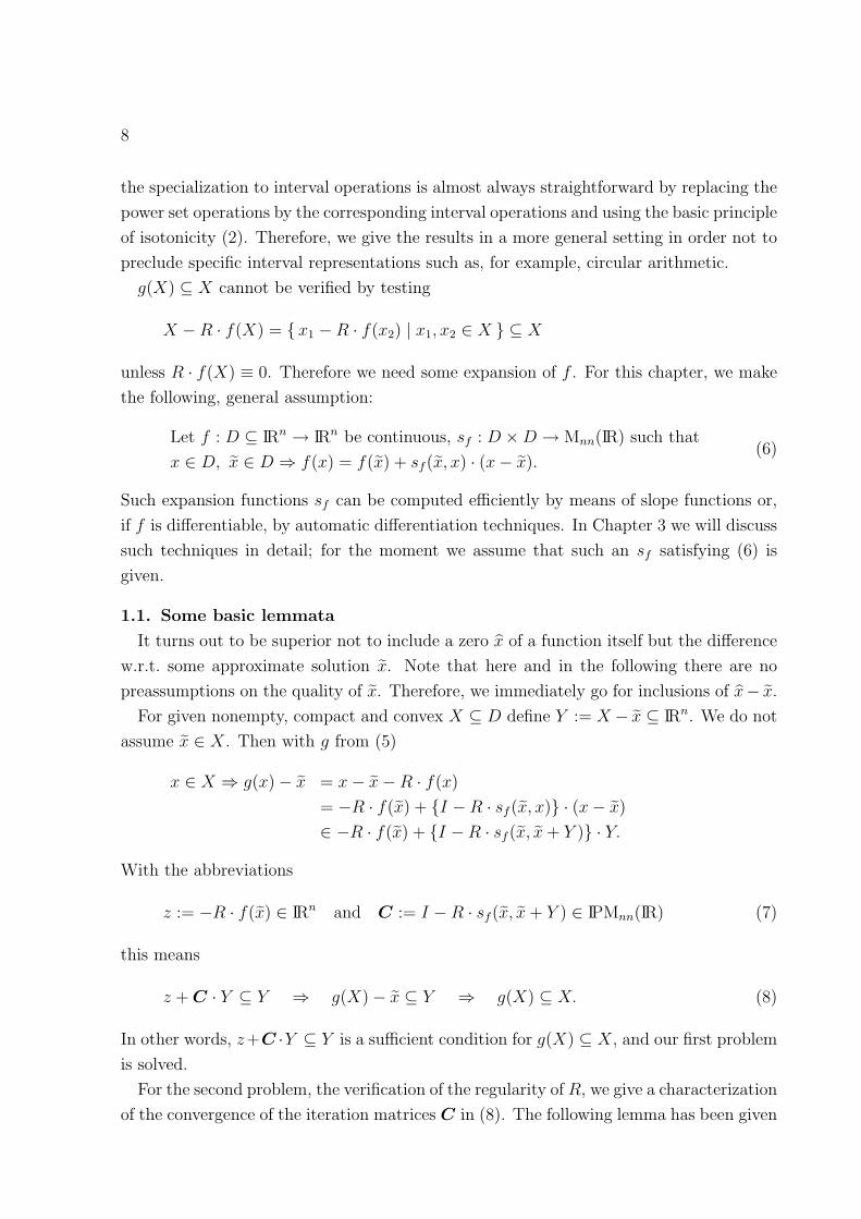
On the other hand, σn(A) = 1 and σ1(∆) = n, implying ω(A, ∆) ≥ n−1 by Theorem 1.8.

If A is an orthogonalized random matrix, then |Aij| . n−1/2. Hence the ratio between the

two estimations on ω(A, ∆) is

(σn(A)/σ1(∆)) / ρ(|A−1|∆)−1 ≈ n−1 · n2 · n−1/2 =√

n.

In other words, for orthogonal matrices Theorem 1.8 verifies regularity of interval matrices

with radius up to a factor of√

n larger than (18). The following table shows that this

ratio is indeed achieved for orthogonalized random matrices.

(σn(A)/σ1(∆)) / ρ(|A−1| ·∆)−1 n = 100 n = 200 n = 500 n = 1000

∆ = |A| 8.3 11.6 18.4 26.0

∆ = (1) 8.3 11.6 18.4 25.9√n 10.0 14.1 22.3 31.6

Table 1.1. Ratio of estimations (20) for ω(A, ∆),

A−1 = A−T random, 50 samples each

2. Dense systems of nonlinear equations

With the preparations of the previous chapter we can state an inclusion theorem for

systems of nonlinear equations. We formulate the theorem for an inclusion set Y which

is an interval vector. A formulation for general compact and convex ∅ 6= Y ∈ IPIRn is

straightforward, following the proof of Theorem 2.1 and using Lemma 1.1.

2.1. An existence test

Theorem 2.1. Let f : D ⊆ IRn → IRn be a continuous function, R ∈ IRn×n, [Y ] ∈IIIRn, x ∈ D, x + [Y ] ⊆ D and let a function sf : D ×D → Mnn(IR) be given with

x ∈ x + [Y ] ⇒ f(x) = f(x) + sf (x, x) · (x− x). (21)

Define Z := −R · f(x) ∈ IRn, C : D → Mnn(IR) with Cx := C(x) = I − R · sf (x, x) and

define [V ] ∈ IIIRn using the following Einzelschrittverfahren for 1 ≤ i ≤ n:

Vi := {3(Z + C x+[U ] · [U ] }i with [U ] := (V1, . . . , Vi−1, Yi, . . . , Yn)T . (22)

If

[V ] $ [Y ], (23)

then R and every matrix C ∈ C x+[V ] are regular, and there exists some x ∈ x + [V ] with

f(x) = 0.

Remark. The interval vector [U ] in (22) is defined individually for every index i

(see (13)). For better readability we omit an extra index for [U ] and use Vi and [V ]i

17

synonymously.

Proof. Define g : D → IRn by g(x) := x − R · f(x) for x ∈ D. The definition (22) of

[V ] together with (23) yields

3(Z + C x+[V ] · [V ]) ⊆ [V ].

Hence, for all x ∈ x + [V ] we have by (23) and (21)

g(x) = x−R · f(x) = x−R · {f(x) + sf (x, x) · (x− x)}= x−R · f(x) + {I −R · sf (x, x)} · (x− x)

∈ x−R · f(x) + {I −R · sf (x, x + [V ])} · [V ]

⊆ x + Z + C x+[V ] · [V ]

⊆ x + [V ],

that is, g is a continuous mapping of the nonempty, convex and compact set x + [V ] into

itself. Thus Brouwer’s Fixed Point Theorem implies the existence of some x ∈ x + [V ]

with g(x) = x = x− R · f(x), and hence R · f(x) = 0. Lemma 1.3 implies the regularity

of R and every matrix C ∈ C x+[V ] which in turn yields f(x) = 0 and demonstrates the

theorem.

Theorem 2.1 implies 3(Z + C x+[V ] · [V ]) ⊆ [V ], not necessarily with $. The interesting

point in using the Einzelschrittverfahren is that the set of iteration matrices C x+[U ] is not

fixed but shrinks in every step. Therefore, (23) may be satisfied, whereas Z+C x+[Y ] ·[Y ] $

[Y ] is not true. So the Einzelschrittverfahren is a convergence accelerator. For examples,

see table 2.1.

We want to stress that f is only required to be continuous; no differentiability assump-

tion is required. Also, the only assumption on the function sf is (21). Moreover, we only

conclude existence, and not uniqueness of the zero x within x + [V ]. On the other hand,

we need the expansion (21) of f only w.r.t. x. Note that we do not require x ∈ x + [V ].

Those facts are demonstrated in the following simple example. Define

f(x) :=

|x| · sin(1/x) for x 6= 0

0 for x = 0.(24)

f is continuous on the whole real axis. We set x := 0.7, [Y ] := [−3.2,−0.2]. Note that [Y ]

should contain the difference of a zero of f and x. Then the slope condition (21) reads

x ∈ [−2.5, 0.5] ⇒ f(x) = f(x) + sf (x, x) · (x− x).

One can show (see Figure 2.1) that [S] := [0.5, 2] satisfies

x ∈ [−2.5, 0.5] ⇒ f(x) ∈ f(x) + [0.5, 2] · (x− x)

18

demonstrating the existence of such a function sf . Of course, the usual approach would

be to compute a function sf and from that the interval [S]. For a large class of functions

this process can be automized as will be discussed in Chapter 3. Then, setting R := 0.5,

we have

−R · f(x) + {1−R · sf (x, x + [Y ])} · [Y ]

⊆ [−0.35,−0.34] + {1− 0.5 · [0.5, 2]} · [−3.2, 0.2]

⊆ [−0.35,−0.34] + [0, 0.75] · [−3.2, 0.2]

⊆ [−2.75,−0.34] $ [Y ] = [−3.2,−0.2]

This demonstrates by Theorem 2.1 that R 6= 0 and s 6= 0 for all s ∈ S and the existence

of some x ∈ x + [−2.75,−0.34] = [−2.05, 0.36] with f(x) = 0. In our example, we have in

fact infinitely many zeros, a point, where f is non-differentiable as well as infinitely many

zeros of f ′ within the inclusion interval [−2.05, 0.36].

-2.5 -2 -1.5 -1 -0.5 0 0.5 1-1

-0.8

-0.6

-0.4

-0.2

0

0.2

0.4

0.6

0.8

slope 0.5 slope 2

|

x~

Figure 2.1 Graph of |x| · sin 1/x with slopes

In one dimension, by its definition the function sf must be continuous except in x. This

changes for n ≥ 2. There, the matrix function sf (x, x) needs only be continuous “in the

direction x− x”; otherwise discontinuities may occur. The definition of sf (x, x) for x = x

is almost arbitrary; any matrix value within C x+[V ] does not influence the assumptions

of Theorem 2.1. In fact, the set sf (x, x + [Y ]) need not even be connected.

The example above is, of course, an artificial example to demonstrate some basic obser-

vations concerning Theorem 2.1. In a practical application the diameter of [Y ] is usually

small compared to the absolute value of x, and this is advantageous in order to obtain

19

accurate inclusions. For comparing different methods consider the original Krawczyk

operator [52]

K([X]) := x−R · f(x) + {I −R · f ′([X])} · ([X]− x),

where f is supposed to be in C1 and f ′([X]) is an interval evaluation of the Jacobian of

f , the latter, for example, obtained by automatic differentiation (see [69], [26]). Then

the proof of Theorem 2.1 shows that g(x) ∈ K([X]) for all x ∈ [X] provided x ∈ [X].

Furthermore K([X]) $ X implies the existence of some x ∈ [X] with f(x) = 0. Use of the

Jacobian as slope function expands f within [X] w.r.t. every x ∈ [X], not only w.r.t. x.

This also yields the uniqueness of x within [X] (cf. also Theorem 2.3). We now compare

the following two algorithms:

Given R, x do

I) [Z] := x−R · f(x); [X] := [Z]; k = 0;

repeat

k = k + 1;

[Y ] := hull(x, [X] ◦ ε);

[C] := I −R · f ′([Y ]);

[X] := [Z] + [C] · ([Y ]− x);

until [X] $ [Y ] or k = 15;

if [X] $ [Y ] then

∃1−1x ∈ [X] : f(x) = 0

II) [Z] := −R · f(x); [X] := [Z]; k = 0;

repeat

k = k + 1;

[Y ] := hull(0, [X] ◦ ε);

[C] := I −R · f ′(x + [Y ]);

[X] := [Z] + [C] · [Y ];

until [X] $ [Y ] or k = 15;

if [X] $ [Y ] then

∃1−1x ∈ x + [X] : f(x) = 0

Finally, we compare with a third algorithm which is

III) algorithm II) using an Einzelschrittverfahren.

The computing times for all three algorithms are roughly the same provided the same

number of iterations is performed. For good approximations R ≈ f ′(x)−1 and x with

f(x) ≈ 0 all three algorithms perform similarly, in the number of iterations as well as in the

accuracy of the inclusion intervals. We are interested in the effect of bad approximations

R and x, the quality of which we do not know a priori. In practice, if the problem is not

too ill-conditioned, a few Newton iterations can improve the quality of an approximate

solution, and therefore we can usually assume x to be fairly good. The quality of R,

however, may be poor if it originates from inverting f ′(x) with a poor starting value x.

Moreover, improving R is expensive, and therefore one might try a verification step with

the given one.

20

Consider the following example by Branin (cf. [1])

f1 = 2 sin(2π x1/5) · sin(2 π x3/5)− x2

f2 = 2.5− x3 + 0.1 · x2 · sin(2 π x3)− x1

f3 = 1 + 0.1 · x2 · sin(2 π x1)− x3

with a solution x = (1.5, 1.809 . . . , 1.0)T . All of the following computations are performed

in single precision (∼ 7 decimal digits).

number of iterations relative accuracy

algorithm δ average maximum average minimum # failed

I) 0.001 1 1 1.6e-6 2.6e-6 0

II) 0.001 1 1 1.2e-6 1.6e-6 0

III) 0.001 1 1 1.2e-6 1.6e-6 0

I) 0.1 1 1 2.4e-5 7.4e-5 0

II) 0.1 1 1 1.6e-6 2.8e-6 0

III) 0.1 1 1 1.4e-6 2.3e-6 0

I) 0.25 1 1 5.9e-5 1.7e-4 0

II) 0.25 1 1 2.3e-6 4.5e-6 0

III) 0.25 1 1 1.8e-6 3.4e-6 0

I) 0.5 1.4 3 1.4e-4 7.2e-4 0

II) 0.5 1.6 3 4.7e-6 2.9e-5 0

III) 0.5 1.3 2 3.1e-6 1.2e-5 0

I) 0.75 2.9 13 4.1e-4 4.2e-3 0

II) 0.75 2.4 5 1.5e-5 2.9e-4 0

III) 0.75 1.9 4 7.8e-6 9.9e-5 0

I) 1.0 4.9 15 7.4e-4 7.5e-3 19

II) 1.0 3.6 11 3.3e-4 3.8e-2 11

III) 1.0 3.0 7 7.0e-5 2.7e-3 8

Table 2.1 Comparison algorithms I, II, III

For all three algorithms we performed 2 Newton steps from the starting value (0, 0, 0)T

given in Branin’s example. This produces an x with a relative accuracy 10−7, which is

almost working precision. Then R is computed by

Rij = {f ′(x)−1}ij · (1 + δ · randij)

where δ is the perturbation parameter and randij are uniformly distributed random num-

bers in [−1, 1]. In the following table we display the average and maximum number of

21

interval iterations necessary (the k in the algorithm), average and minimum relative ac-

curacy w.r.t. the midpoint of the components of the computed inclusion interval, and the

number of cases in which no inclusion was achieved. For every perturbation value δ for

R we performed 100 test runs.

The comparison of the three algorithms depends, of course, very much on the problem

to solve and on the choice of ε. The first algorithm computes an inclusion of the solution

itself; therefore we have to choose a small ε to allow convergence and to keep a good relative

accuracy. In our test results we used a relative inflation by 10−5 for the first algorithm.

The second and third algorithm enclose the error w.r.t. x; therefore a reasonable inflation

is necessary. In the example we took 20 % relative inflation. In all three algorithms, we

expanded the interval adding twice the smallest positive machine number, thus taking the

second predecessor, successor of the left, right bound, respectively.

The table shows that for smaller δ (up to 25 %), all algorithms use 1 interval iteration.

Enclosing the error rather than the solution gains little for a good approximation R but

more than one figure for δ = 0.25. Remember that the value of δ is a maximum of random

perturbations for R. For larger δ the third algorithm needs the smallest number of interval

iterations whereas for a maximum of 100 % perturbation the number of failures is best

for the third algorithm. The number of iterations is important w.r.t. the computing time

because every iteration requires the evaluation of a Jacobian and the multiplication by

R. Another interesting approach to construct a starting region [X] for nonlinear systems

is described by Alefeld [6].

2.2. Refinement of the solution

If an inclusion is not good enough, iterative refinement using intersection is possible.

For the sake of completeness we state the following theorem. However, we do not recom-

mend extensive use of this technique. In most cases a pure floating point iteration with

subsequent verification step will be more efficient, in terms of computing time as well as

accuracy.

Theorem 2.2. With the assumptions of Theorem 2.1, assume [V ] $ [Y ]. Then x ∈x + [V ], and if the i-th component Vi of [V ], 1 ≤ i ≤ n is replaced by

Vi := Vi ∩ {3 (Z + C x+[V ] · [V ])}i,

then x ∈ x + [V ] still holds true for the new [V ]. In other words, continuing with the

Einzelschrittverfahren described in Theorem 2.1 together with componentwise intersection

no zero of f can be lost. If, with the assumptions of Theorem 2.1 except (23)

Vi ∩ {3 (Z + C x+[U ] · [U ])}i = ∅ for [U ] := (V1, . . . , Vi−1, Yi, . . . , Yn)T

22

for some 1 ≤ i ≤ n, then x + [Y ] contains no zero of f .

Proof. Following the proof of Theorem 2.1 every zero x ∈ x + [V ] is a fixed point

of g and is therefore contained in 3(Z + C x+[V ] · [V ]) which proves the first part of the

theorem. Using g(x) ∈ Z + C x+[Y ] · [Y ] for all x ∈ x + [Y ] proves the second part.

2.3. Verification of uniqueness

We have proven existence of a zero within a given interval, but not uniqueness of this

zero. The latter can be verified by the following theorem.

Theorem 2.3. With the assumptions of Theorem 2.1, assume [V ] $ [Y ], i.e. there exists

some x ∈ x + [V ] with f(x) = 0. For a given interval vector [W ] ⊇ [V ], x + [W ] ⊆ D, let

the function sf satisfy

y ∈ x + [W ] ⇒ f(y) = f(x) + sf (x, y) · (y − x) for all x ∈ x + [V ] (25)

in addition to (21).

If all S ∈ sf (x + [V ], x + [W ]) are regular, then the zero x of f is unique in x + [W ].

Proof. For y ∈ x + [W ] with f(y) = 0, (25) implies

0 = f(y) = f(x) + sf (x, y) · (y − x) = sf (x, y) · (y − x)

and the regularity of sf (x, y) implies y = x.

The regularity of the set of matrices sf (x + [V ], x + [W ]) can be verified by means of

Lemma 1.1 or 1.3. In the latter case it is simpler to use Lemma 1.6, which saves a lot

of computing time. Computing large inclusion intervals containing exactly one solution

is important, for example, in global optimization (see [38]) or, for verified computation

of all zeros of a nonlinear system within a given domain [48]. For large banded or sparse

matrices, Theorem 1.8 can be used to prove regularity.

2.4. Verification of existence and uniqueness for large inclusion intervals

In a practical implementation it can be advantegeous first to verify existence in a small

solution set x + [V ] and then to verify uniqueness in a much larger one x + [W ]. This

two-step approach is superior to trying to verify existence and uniqueness in one step for

the larger set x + [W ].

23

x~ + [W]

x~ + [V]

Figure 2.2 Verifying existence in x + [V ] and uniqueness in x + [W ]

This is because we would need to expand f(x) w.r.t. every point in the large set x + [W ]

which makes the set of matrices sf (x+[W ], x+[W ]) very thick and possibly not convergent.

Given a “large” set x + [W ] in which we want to verify existence and uniqueness of a

zero x of f we can proceed as follows:

1. Compute an approximate solution x

2. Compute some x + [V ] with x ∈ x + [V ] of small size near x using Theorem 2.1

3. Possibly refine x + [V ] using Theorem 2.2

4. Verify regularity of sf (x + [V ], x + [W ]) using Lemma 1.6

Algorithm 2.1 Verification of existence and uniqueness within large intervals

We add some practical remarks on the above algorithm:

• The approximation x should be good. Very much in the sense of Wilkinson (0.3)

we do as much as possible in floating point. It is better and faster. It remains the

task for interval analysis to verify the quality of an approximation.

• The inclusion interval x + [V ] should be of good quality. However, rather than

applying 1 iteration in step 3 it is better to perform 2 iterations in step 1 (if x was

not good enough).

• In step 4 only regularity of the interval matrix [C] := sf (x + [V ], x + [W ]) is to

be verified. The fundamental advantage of the above algorithm is that this [C]

is constant. That means, applying Lemma 1.6 and Theorem 1.5 leads to the ver-

ification existence and uniqueness of the zero of f within x + [W ] if and only if

ρ(|I −R · [C]|) < 1.

Furthermore, it is much faster than applying Theorem 2.1 directly to x + [W ] be-

cause if an iteration has to be performed, the matrix sf (x + [W ], x + [W ]) has to

be recomputed and the multiplication by R has to be executed in every step. This

means computation of a whole Jacobian or slope, and a matrix times interval ma-

trix product. In contrast, Algorithm 2.1 needs only a real matrix times real vector

multiplication in each iteration step when using Lemma 1.6.

24

In other words, we can expect to obtain verification of existence and uniqueness faster

and within larger intervals using Algorithm 2.1. This can be of great importance in

practical applications. For example, in global optimization many refinements can possibly

be saved, especially in higher dimensions.

We illustrate the use of Algorithm 2.1 with a simple one-dimensional example. Let

f(x) := ex − 2x− 1 (26)

with f(0) = 0, x := 0.1 and x + [Y ] := [−0.1, +0.1]. The slope in the one-dimensional

case is the set of secants s(x, x) := {f(x)− f(x)}/(x− x) for x 6= x, and it is easy to see

that

[S] := { s(x, x) | x ∈ x + [Y ], x 6= x } = [s(0.1,−0.1), s(0.1, 0.1)] ⊆ [−1.0,−0.89].

Setting R ≈ mid([S])−1 = −0.945−1, e.g. R := −1 yields

−R · f(x) + {1−R · [−1,−0.89] } · [−0.1, +0.1] = [−0.106,−0.083] =: [V ]

$ [−0.2, 0] = [Y ]

Therefore, there is a zero x of f within x + [V ] = [−0.006, +0.017], namely x = 0. Up to

now we do not know uniqueness. Consider x + [W ] := [−2, 1]. Then the set of secants

computes to

{ s(x, y) | x ∈ x + [V ], y ∈ x + [W ], y 6= x } = [s(−0.006,−2), s(0.017, 1)]

= [−1.570,−0.269]

which does not contain zero and therefore implies the uniqueness of x = 0 in the larger

interval [−2, 1]. On the other hand the slope function for x + [W ]

{ s(x, y) | x, y ∈ x + [W ], x 6= y } ⊆ [−1.8647, +0.7183]

contains 0 and is therefore not suitable for an inclusion. Even if we take x := x = 0 and

[Y ] := x + [W ] = [−2, 1] we cannot even verify existence of a zero within [−2, 1], because

{ s(0, x) | x ∈ [−2, 1], x 6= 0 } ⊆ [−1.5677,−0.2818] =: [S], and taking R := mid([S])−1 =

−1.0814 yields

−R · f(x) + {1−R · [S]} · [W ] = {1 + 1.0814 · [−1.5677,−0.2818]} · [−2, 1]

⊆ [−1.391, +1.391] 6⊆ [−2, 1].

We want to add two remarks to the previous example. First, in our computation of

s(x, y), we always assumed x 6= y. This is because we calculated s directly from the

set of secants which is undefined for x = y. On the other hand, the assumptions of our

theorems are always assumptions on an expansion of f like (25). Therefore the values

sf (x, y) for x = y are uninteresting, because in this case f(x) = f(y). Therefore, we

25

could exclude these values in the assumptions of our theorems. On the other hand, in a

practical application this in turn is unimportant, and for the sake of better readability we

did not exclude x = y. The second remark concerns the computation of the function sf ,

which was simple in the previous example and essentially done by hand using auxiliary

information of the function f . In Chapter 3 we will discuss a method for automatic

evaluation of such funtions sf for a wide class of functions f .

In the case of functions depending on data which are afflicted with tolerances, we can

use parametrized functions with parameters varying within a certain tolerance. It is

straightforward to give theorems corresponding to Theorems 2.1, 2.2 and 2.3 for this case.

However, in this case the solution is not a single point, but we have a whole set of solutions

corresponding to parameters within the tolerances. Then we obtain an inclusion of this

solution set, which is, by the principles of interval analysis, an outer inclusion, i.e. a set

which is verified to contain the solution set. However, it is important to know whether

this inclusion is possibly an overestimation of the true solution set or not.

2.5. Inner inclusions of the solution set

The amount of overestimation can be estimated by means of inner inclusions. For some

set Σ ∈ IPIRn we call [X] ∈ IIIRn an inner inclusion if for every component 1 ≤ i ≤ n,

infσ∈Σ

σi ≤ inf([X])i and sup([X])i ≤ supσ∈Σ

σi

holds. In other words, for every component [X]i of [X], there are points in Σ the i-th

component of which are left of the lower bound of [X]i and right of the upper bound of

[X]i, respectively. Such inner bounds for the solution set of a parametrized system of

nonlinear equations can be computed by means of the following theorem. Note that these

are bounds for the solution set for finite perturbations of parameters within some set of

parameters C.

Theorem 2.4. Let f : Dp×Dn ⊆ IRp× IRn → IRn be continuous w.r.t. the unknowns

x ∈ IRn, let R ∈ IRn×n, [Y ] ∈ IIIRn, x ∈ Dn with x + [Y ] ⊆ Dn, and for C ∈ IPIRp,

C ⊆ Dp let a function sf : Dp ×Dn ×Dn → Mnn(IR) be given with

c ∈ C, x ∈ x + [Y ] ⇒ f(c, x) = f(c, x) + sf (c, x, x) · (x− x). (27)

Define Z := −R·f(C, x) ∈ IPIRn, C : Dp×Dn → Mnn(IR) with C(c, x) := I−R·sf (c, x, x)

and define [V ] ∈ IIIRn using the following Einzelschrittverfahren:

1 ≤ i ≤ n : Vi := {3(Z + C(C, x + [U ]) · [U ])}i

with [U ] := (V1, . . . , Vi−1, Yi, . . . , Yn)T .(28)

If

[V ] $ [Y ], (29)

26

then R and every matrix within C(C, x + [V ]) is regular, and for every c ∈ C there

exists some xc ∈ x + [V ] with f(c, xc) = 0. Define the solution set Σ of f within x + [Y ]

w.r.t. parameters c ∈ C by

Σ := {x ∈ x + [Y ] | ∃ c ∈ C : f(c, x) = 0 }. (30)

Then Σ ⊆ x + [V ], and abbreviating

[Z] := 3(Z) and [∆] := 3(C(C, x + [V ]) · [V ]),

the following componentwise estimations hold true

xi + inf([Z]i) + sup([∆]i) ≥ infσ∈Σ

σi and

xi + sup([Z]i) + inf([∆]i) ≤ supσ∈Σ

σi.(31)

Proof. The first part of the theorem follows by applying Theorem 2.1 for every c ∈ C.

Let c ∈ C be fixed but arbitrary. Then defining g : Dn → IRn by g(x) := x− R · f(c, x),

following the first part of the proof of Theorem 2.1, and using (28) and (29) for 1 ≤ i ≤ n

we see that every fixed point of g within x + [Y ] needs also to be in x + [V ]. But every

zero of f is a fixed point of g, hence Σ ⊆ x+[V ]. For c ∈ C we have for every x ∈ x+[Y ]

x−R · f(c, x) = x−R · {f(c, x) + sf (c, x, x) · (x− x)}= x−R · f(c, x)− {I −R · sf (c, x, x)}(x− x).

For this c ∈ C there exists some xc ∈ x + [V ] ⊆ x + [Y ] with f(c, xc) = 0 and

x−R · f(c, x) = xc − {I −R · sf (c, x, xc)}(xc − x)

∈ Σ−C(C, x + [V ]) · [V ]

⊆ Σ− [∆].

(32)

The left hand side of (32) is an element of x + Z. Since c ∈ C was choosen arbitrarily we

also have

x + Z ⊆ Σ− [∆] or ∀ z ∈ Z ∃ σ ∈ Σ ∃ δ ∈ [∆] : x + z = σ − δ. (33)

For fixed index i between 1 and n and every ε > 0, there is a c ∈ C with

{−R · f(c, x)}i ≤ inf([Z]i) + ε.

Together with (33) this shows the existence of some c ∈ C, σ ∈ Σ and δ ∈ [∆] with

x + inf([Z]i) + ε ≥ {x−R · f(c, x)}i = σi − δi ≥ infσ∈Σ

σi − sup([∆]i)

27

and proves the first inequality. The second one follows similarly.

In a practical application the sharpness of the bounds depends on [∆]: this is exactly the

difference between the inner and outer bounds. But [∆] is the product of I−R ·sf (C, x+

[V ]) and [V ]. The first factor is small for R ≈ sf (c, x)−1 for some c ∈ C and diameter

of C not too big, and the second factor [V ] is the difference between x and the solutions

xc, and therefore also small. In other words, [∆] is the product of small quantities for

reasonable parameter tolerances. This means we can expect inner and outer bounds not

too far apart.

We give a simple example. We use the nonlinear system given by Broyden [16] which

we parametrize with 3 parameters:

p1 · sin(xy)− y / (4π)− x / p2 = 0

(1− 1 / (4π)) · (ep3·x − e) + ey / π − 2ex = 0(34)

with initial approximation (0.6,3) and parameter values

p1 ∈ 0.5 · [1− ε, 1 + ε]

p2 ∈ 2.0 · [1− ε, 1 + ε] for ε = 0.01 in all 3 cases.

p3 ∈ 2.0 · [1− ε, 1 + ε]

For the midpoint parameter value (0.5, 2, 2)T we have a solution x = (0.5, π). For the

expansion of the function f we use slopes, not the Jacobian. The latter gives poorer

results as will be discussed in the next chapter. After a short computation, choosing

x ≈ x, we obtain

[Z] ⊆ [−0.01819, +0.01814]

[−0.03389, +0.03358]

, [∆] ⊆

[−0.0052, +0.0052]

[−0.0071, +0.0072]

and

Σ ⊆ [0.4766, 0.5233]

[3.1006, 3.1823]

.

Automated evaluation of the slope function sf will be discussed in the next chapter. The

problem in applying (31) is that outer bounds for [∆] suffice, but we need inner bounds

for [Z]. We could regard [Z] as a good approximation for 3 Σ with error term [∆]. For

linear systems the determination of inner bounds of [Z] is not too difficult, as we will see

in Chapter 4.

In the nonlinear case we could compute −R · f(c, x) for several random c ∈ C and

take the interval hull. This yields, especially for larger dimensions, very poor results

28

(an example for linear systems is given in Chapter 4). If f is differentiable w.r.t. the

parameters c, a better method is to locally linearize:

R · f(c, x) ≈ R · f(c, x) +

{R · ∂f

∂c(c, x)

}· (c− c).

If C = [C] is a parameter interval and c its midpoint, then the matrix R · ∂f∂c

(c, x) is the

local steepest descent direction. If we take c ∈ ∂[C] with

sign(c− c)j = ± sign(R · ∂f

∂c(c, x))ij, (35)

we have the locally best choices of c for the i-th component of [Z]. In our example it is

R · ∂f

∂c(c, x) ≈

−1.9 −0.2 −0.2

−0.9 −0.1 1.3

and the corresponding values for −R · f(c, x) are

−0.01818

0.01968

,

0.01813

−0.01999

,

−0.00965

−0.03388

,

0.00960

0.03357

,

for c according to (35). Thus

[Z] ⊇ [−0.01818, +0.01813]

[−0.03388, +0.03357]

.

If only the elongation of few solution components is needed, the nonlinear system can be

solved using the specific parameters computed by (35).

The matrix ∂f∂c

(c, x) can be computed in an automated process by means of automatic

differentiation [69], [26]. If f is not differentiable w.r.t. the parameters c, slopes instead

of derivatives can be used as well.

Finally, applying Theorem 2.4 we obtain

[0.4870, 0.5130]

[3.1149, 3.1680]

⊆ 3 (Σ) ⊆

[0.4766, 0.5233]

[3.1006, 3.1823]

which still gives reasonable accuracy for practical purposes. In the following figure the

dashed rectangle is [Z], the dotted one is the inner and the solid one is the outer inclusion

for 3(Σ), whereas the circles depict actual zeros of f(c, x) for components ci of the

parameter c varying independently in an arithmetic progression between the bounds.

29

0.47 0.48 0.49 0.5 0.51 0.52 0.53

3.1

3.12

3.14

3.16

3.18

3.2

Figure 2.3 Inner and outer inclusions of the solution complex

Obviously [Z] is a good approximation of 3(Σ). It should be noted that with the

assumptions of Theorem 2.4, we do not assure uniqueness of the zero of f(c, x) for fixed

parameter c ∈ C within x + [V ]. Therefore the solution complex need not be connected.

For ε larger than 0.015, the nonlinearities over the whole parameter domain become

too big, and other techniques like bisection have to be used to obtain an inclusion.

Inner inclusions in the above sense were first investigated by Neumaier [65]. In com-

parison, the computation of inner inclusions using the methods described above is much

cheaper. The above Theorem 2.4 was proved for Jacobians instead of slopes in [79].

As a larger, dense example consider

discretization of u(t) +1∫0

H(s, t) · (p · u(s) + s + 1)3ds = 0

with p ∈ [0.9, 1.1] and H(s, t) =

s(1− t) for s ≤ t

t(1− s) for s > t

(36)

proposed by More and Cosnard [62]. This produces a problem with full Jacobian matrix.

For dimension n = 1000 we obtained the following results. The inner and outer inclusions

30

for all 1000 components are of the same quality as those shown below.

[−0.00085, −0.00081] ⊆ [X]1 ⊆ [−0.00089, −0.00077]

[−0.00170, −0.00163] ⊆ [X]2 ⊆ [−0.00178, −0.00155]

. . .

[−0.00353, −0.00340] ⊆ [X]999 ⊆ [−0.00364, −0.00328]

[−0.00176, −0.00170] ⊆ [X]1000 ⊆ [−0.00182, −0.00164]

Table 2.2. Inner and outer inclusion for (36) and dimension n = 1000

2.6. Sensitivity analysis with verified inclusion of the sensitivity

Computing inner inclusions for the solution set of a parametrized system of nonlinear

equations yields a sensitivity analysis for finite perturbations of the input parameters.

If we are interested in the sensitivity for a specific parameter value, we have to use

other techniques. The difference to the previous approach is that we are looking for the

sensitivity of the solution w.r.t. ε-perturbations in the limit ε → 0.

For a meaningful definition of the sensitivity of a zero xc, f(c, xc) = 0 of a function f

w.r.t. perturbations of a parameter c, we locally need continuous dependency of xc on c.

Using an inclusion computed by means of Theorem 2.1 does not assure this. Consider for

example |x| + c2 for c = 0. Therefore we impose stronger assumptions on f . Moreover,

we use a Jacobian-like function instead of sf .

Theorem 2.5. Let f : Dp × Dn ⊆ IRp × IRn be twice differentiable w.r.t. both the

parameters Dp and unknowns Dn, such that for each parameter cj at most one component

function fi is dependent on cj. Let x ∈ Dn, R ∈ Mnn(IR), [Y ] ∈ IIIRn such that x + [Y ] ⊆Dn. Define

J(c,X) := 3 { ∂f

∂x(c, x) | x ∈ X } (37)

for X ∈ IPIRn, X ⊆ Dn, c ∈ Dp. For fixed parameter c ∈ int(Dp), let Z := −R · f(c, x)

and let C([U ]) := I −R · J(c, x + (0 ∪ [U ])). Define [V ] ∈ IIIRn by means of the following

Einzelschrittverfahren

1 ≤ i ≤ n : Vi := {Z + C([U ]) · [U ]}i with [U ] := (Vi, . . . , Vi−1, Yi, . . . , Yn)T .

Then

[V ] $ [Y ]

implies the existence of a unique and simple zero xc of fc(x) = f(c, x) within x+ [V ]. Let

c∗ ∈ IRp, c∗ ≥ 0 and define

u := |R| · |∂f

∂c(c, x)| · |c∗|

w := |I −R · J(c, x + (0 ∪ [V ]))| · d[V ].

31

Then

φ := maxi

ui

(d[V ]− w)i

is well defined. For small enough ε > 0 and for every c with |c − c| ≤ ε · c∗, there is a

uniquely defined zero xc of fc within x + [V ], and the sensitivity vector of the zero xc of

fc w.r.t. perturbations weighted by c∗ can be defined componentwise by

Sens(xc, f, c∗)k := limε→0+

max { |xc − xc|kε

: |c− c| ≤ ε · c∗ }.

The sensitivity vector satisfies

Sens(xc, f, c∗) ∈ [u− φ · w, u + φ · w].

Proof. Theorem 2.4 implies the existence and uniqueness of a zero xc of fc. This zero

must be simple because of the regularity of the corresponding Jacobian which is implied

by (37) and Theorem 2.4. Hence Z + C([V ]) ⊆ [V ]. Now the proof of Theorem 2.4 in

[80], which is lengthy and therefore omitted here, can be followed.

It should be mentioned that x occuring in the definition of u can be replaced by x +

[V ], and the derivative w.r.t. the parameters can easily be computed using automatic

differentiation in a forward or backward mode (cf. [26] or [69]).

The true sensitivity can be shown (cf. [80]) to be equal to

Sens(xc, f, c∗) =

∣∣∣∣∣∣

(∂f

∂x(c, x)

)−1∣∣∣∣∣∣·∣∣∣∣∣∂f

∂c(c, x)

∣∣∣∣∣ · c∗. (38)

The main point of the above theorem is that the inverse Jacobian does not have to be

included, but information from the inclusion process suffices to bound the difference be-

tween R and the true inverse of the Jacobian and finally to include the sensitivity. Bounds

using absolute values have been investigated by Bauer [12]. Formula (38) verifies sensitiv-

ity results on linear systems by Skeel [86] and for matrix inversion and linear programming

problems given by Rohn [72]. For many other standard problems in numerical analysis,

(38) allows to state simple explicit formulas for the sensitivity. Using the verification

scheme, inclusions of the sensitivity can also be computed (see [80]).

One main advantage of the approach we chose in Theorem 2.5 is that we are free

to choose the weights c∗. A weight c∗i = |ci| imposes a relative perturbation, a weight

c∗i = 1 an absolute perturbation and, especially, c∗i = 0 imposes no perturbation at all

for the parameter ci. This is important in practical applications when ci is some system

parameter like a system zero which need not be perturbed by construction. This is a main

advantage over a norm approach.

32

3. Expansion of functions and slopes

In this chapter we follow two aims: to derive algorithmic principles for estimating the

range of a function f over a domain X, and to expand f over X w.r.t. some point x. For

differentiable f : IRn → IR this can be achieved by using the n-dimensional mean value

theorem. For [X] ∈ IIIRn,

∀ x, y ∈ [X] : f(x) ∈ f(y) + [J ] · (y − x) (39)

shows that [J ] :=⋂{ [M ] ∈ IIMnn(IR) | ∂f

∂x(x) ∈ [M ] for all x ∈ [X] } allows an expansion

w.r.t. every y ∈ [X]. The inclusion theorems given in Chapter 2 only require an expansion

w.r.t. a single point x. In turn this allows to prove existence but not uniqueness, the latter

being verified with Theorem 2.3. Moreover, we do not want to restrict our functions to

the class of differentiable ones, and we do not require x ∈ [X].

(39) shows that ∂f∂x

could serve as an expansion function. However, when applying the

theorems of Chapter 2 to problems with high-nonlinearity or for the verification of large

inclusion intervals, we are interested in expansion intervals of small diameter. For our

example (2.6) we obtain for [X] = [−2, 1]

f ′([X]) = e[X] − [2] ⊆ [−1.865, 0.719],

which covers all slopes within [X] w.r.t. every x ∈ [X] rather than, e.g., the slopes

[S] = [−1.568, −0.281] w.r.t. the single point x = 0. Moreover, in our example f ′([X])

contains zero and is therefore not useful for our verification purposes. For n-dimensional

functions we can shrink the diameter slightly by observing that for [X] ∈ IIIRn, x ∈ IRn

and f : IRn → IRn ∈ C1,

∀ x ∈ [X] : f(x) ∈ f(x) + Z · (x− x) with

Zij :=∂fi

∂xj

(X1, . . . , Xi−1, xi ∪ Xi, xi+1, . . . , xn) (40)

holds. This was used by Hansen [28], see also Alefeld [4]. Using this also loses uniqueness

of the zero. It helps, but more can be done. We are aiming for a simple method, easily

and automatically executable on the computer, for computing an enclosure of the slopes

of f w.r.t. a fixed point x. More precisely, we mean the following.

Definition 3.1. Let f : D ⊆ IRn → IR be given. We say that sf ∈ IPIRn expands f

within X ∈ IPIRn, X ⊆ D w.r.t. x ∈ D if

∀ x ∈ X : f(x) ∈ f(x) + sf · (x− x). (41)

33

The set sf depends on x and [X]. We formulate the definition for power set operations,

but due to the basic principle of interval operations, the isotonicity, we immediately have

(41) ⇒ f(x) ∈ f(x) 3+ 3 {sf · ([X] 3− x)} for [X] := 3(X).

Using power set operations simplifies statements and proofs, but does not restrict the

domain of applicability or the assertions when going to interval operations. In order to

formulate a simple implementation scheme we need the following definition.

Definition 3.2. Let f : D ⊆ IRn → IR, X ∈ IPIRn with X ⊆ D and x be given. We

say that the triplet (fc, fr, sf ) ∈ IPIR × IPIR × IPIRn is a slope expansion of f w.r.t. X

and x if

f(x) ∈ fc, f(X) ⊆ fr and sf expands f within X w.r.t. x.

Let a function be given by means of a program using constants, variables, control

structures, loops and so forth. To be more precise we consider a sequence of statements

1 ≤ i ≤ n : zi := xi

n + 1 ≤ i ≤ m : either zi := const or zi := zi1 op zi2 with i1, i2 < i,(42)

where the xi are the values of the independent variables and zm is the value of some

function. Here, op denotes a monadic or dyadic operator to be specified in a moment.

Obviously, many functions can be evaluated using a scheme (42). Next we give a theorem

on how to compute a sequence of slope expansions for such functions.

Theorem 3.3. Let X ⊆ IPIRn, Xi := { ζi | ζ ∈ X } ∈ IPIR and x ∈ IRn be given. Then

with f : IRn → IR:

(xi, Xi, eTi ) is a slope expansion for f(x) ≡ xi (ei denotes the ith unit vector)

(c, c, 0) is a slope expansion for f(x) ≡ c

Given slope expansions (fc, fr, sf ) and (gc, gr, sg) for functions f : IRn → IR and g : IRn →IR, respectively w.r.t. X and x we have

(fc ± gc, fr ± gr, sf ± sg) is a slope expansion for f ± g, resp.

(fcgc, frgr, frsg + gcsf ) is a slope expansion for f · g,

(fc/gc, fr/gr, (sf − fc/gc · sg)/gr) is a slope expansion for f/g

provided the operations are well-defined.

Proof. As an example, we give the calculation for the multiplication, the other opera-

tions follow similarly. For x ∈ X we have

34

(f · g)(x) ∈ f(x) · [g(x) + sg · (x− x)]

⊆ [f(x) + sf · (x− x)] · g(x) + f(x) · sg · (x− x)

⊆ f(x) g(x) + {f(x) · sg + g(x) · sf} · (x− x)

⊆ fc · gc + {fr · sg + gc · sf} · (x− x)

This theorem can be found in [54] and similar ideas are in [30]. In a later paper Neumaier

proved an extension to transcendental functions [64]. Here he showed for example that

(efc , efr , efr · sf ) is a slope expansion for exp ◦ f (43)

provided fc ∈ fr. This can be proved by expanding ef(x) w.r.t. ef(x) for some ζ ∈f(x) ∪ f(x) ⊆ fr

ef(x) = ef(x) + eζ · (f(x)− f(x)) ∈ efc + efr · sf · (x− x)

provided x ∈ X. We can give a sharper slope expansion than (43) not assuming x ∈ X

by means of the following theorem.

Theorem 3.4. Let X ∈ IPIRn and x ∈ IRn be given and let (fc, fr, sf ) be a slope

expansion for f : IRn → IR w.r.t. X and x. For a function g : IR → IR let Sg ∈ IPIRn

expand g within f(X) w.r.t. f(x). Then

(g(fc), g(fr), Sg · sf ) is a slope expansion for g ◦ f w.r.t. X and x.

Proof. (g ◦ f)(x) = g(f(x)) = g(f(x)) + Sg · (f(x)− f(x)) ⊆ g(fc) + Sg · sf · (x− x).

For the set Sg we can take the set of secants within f(X), i.e.

Sg := { g(y)− g(y)

y − y| y := f(x), y ∈ f(X), y 6= y }.

Defining

h(y) :=

{g(y)− g(y)} / (y − y) for y 6= y

g′(y) otherwise

for twice differentiable g, an extremum of h at some y 6= y requires

g′(y) =g(y)− g(y)

y − y.

Then from the mean value theorem we know the existence of some ξ ∈ int(y ∪ y) with

g′(y) = g′(ξ) and for twice differentiable g some ζ ∈ y ∪ ξ ⊆ y ∪ y exists with g′′(ζ) = 0.

35

This proves the following theorem.

Theorem 3.5. For a twice differentiable function g : IR → IR, [X] = [X,X] ∈ IIIR,

x ∈ IR and g′′(x) 6= 0 for all x ∈ x ∪ [X] the set Sg defined by

Sg := h(X) ∪ h(X) with h(x) =

g(x)− g(x)

x− xfor x 6= x

g′(x) otherwise

expands g within [X] w.r.t. x.

For many functions this gives a simple way of computing Sg and therefore a slope

expansion. For locally non-convex or non-concave functions some case distinctions are

necessary.

As an example consider again example (26) with f(x) = ex − 2x− 1 and x = 0, [X] =

[−2, 1]. Then

S :=e−2 − 1

−2∪ e− 1

1⊆ [0.432, 1.719]

expands ex within [X] w.r.t. x = 0 and short computation yields that

(0, [−2.865, 5.719], [−1.568,−0.281]

is a slope expansion of f w.r.t. X and x. This is the same result we used in Chapter 2.

We want to stress that here it is obtained automatically using Theorems 3.3, 3.4, and 3.5.

Computing smaller ranges for the slope is especially interesting in view of the inclusion

Theorems 2.1, 2.3, 2.4 and following, because a necessary condition for the corresponding

assumptions to hold true is the regularity of all s ∈ sf . If we use (43) instead, we obtain

in our example

S ⊆ e[X] · 1 = [e−2, e1] ⊆ [0.135, 2.719],

and a slope expansion

(0, [−2.865, 5.719], [−1.865, 0.719])

for f , with a much bigger slope interval containing zero, thus precluding verification for

[X]. In fact, it is the same as f ′([X]). In other words, Theorem 3.5 allows us to perform

verification of existence and uniqueness according to algorithm 2.1 for larger inclusion

sets.

The verification of uniqueness of a zero using Theorem 2.3 requires expansion of the

function w.r.t. a whole set [Y ] rather than a point x. This can be achieved by replacing

x by [Y ]. The proof uses the fact that a slope expansion is valid for every y ∈ [Y ]. In our

36

example, we needed a slope expansion w.r.t. [−2, 1] and [Y ] := [−0.006, 0.017], the latter

replacing x. We obtain

S :=e−2 − e[Y ]

−2− [Y ]∪ e1 − e[Y ]

1− [Y ]⊆ [0.425, 1.755] (44)

and

[−1.575,−0.245] expands f within [−2, 1] w.r.t. every x ∈ [Y ].

This proves regularity of the slope and therefore, as we have seen before, uniqueness of

the zero of f within [−2, 1]. The slope could be sharpened slightly by using inf([Y ]) and

sup([Y ]) in (44) instead of the entire [Y ]. Then, exactly the results as in Chapter 2 are

obtained.

For Broyden’s example (34) we achieve inclusions up to perturbations ε = 0.015 using

slopes defined by Theorems 3.3 and 3.5. In contrast, using the Jacobian, we only obtained

inclusions for ε not larger than 0.009. This is still true when using the improved version

(40). But even for ε = 0.009 the results obtained by slopes are more accurate. If we denote

the inner inclusion by [S] and the outer inclusion by [T ], then ρi = w([S]i) / w([T ]i) is a

measure for the quality of inner and outer inclusion of the ith component. In our example

we obtained

ρ1 = 0.17, ρ2 = 0.30 using Jacobians (40)

ρ1 = 0.62, ρ2 = 0.70 using slopes defined by Theorems 3.3 and 3.5.

We want to stress again that the process of computing a slope expansion can be fully

automated by means of predefined operators implementing the rules given in the theorems

of this chapter. This is very much in the same spirit as automatic differentiation. We

also mention that slopes can be computed in a backward mode, achieving attractive

computing times as in the case of automatic differentiation. That means computing an

entire slope for a function in n variables takes about 5 times the computing time for

one function evaluation, independent of the number of variables. The possibility of easy

and automatic computation of slopes make them suitable for practical applications. The

computation of slope expansions for functions f : IRn → IRn can be performed for every

component function individually.

4. Dense systems of linear equations

Consider the linear system

Ax = b for A ∈ Mnn(IR), b ∈ IRn

with dense system matrix A. If we regard it as a zero finding problem of f : IRn → IRn,

f(x) = Ax − b we can apply the theorems of Chapters 2 and 3. In the linear case the

37

slope function is constant and equal to the Jacobian, namely A itself:

f(x) = f(x) + A · (x− x) for all x, x ∈ IRn. (45)

Therefore, as an application of Theorem 2.1, we obtain the following result.

Theorem 4.1. Let A ∈ Mnn(IR), b ∈ IRn be given, R ∈ Mnn(IR), [Y ] ∈ IIIRn, x ∈ IRn

and define

Z := R · (b− Ax) ∈ IRn, C := I −R · A ∈ Mnn(IR).

Define [V ] ∈ IIIRn by means of the following Einzelschrittverfahren for 1 ≤ i ≤ n:

Vi := {3(Z + C · [U ])}i where [U ] := (V1, . . . , Vi−1, Yi, . . . , Yn)T . (46)

If

[V ] $ [Y ], (47)

then R and A are regular and the unique solution x = A−1b of Ax = b satisfies x ∈ x+[V ].

Proof. Applying Theorem 2.1 to f(x) = Ax− b yields regularity of R and A and the

existence of some x ∈ x + [V ] with f(x) = 0. x is unique because of the regularity of A.

In the case of linear systems we do not need to use the powerful Theorem 2.1 but

can proceed in a more elementary way. Moreover, convexity of the inclusion set is not

necessary.

Theorem 4.2. Let A ∈ Mnn(IR), b ∈ IRn be given, R ∈ Mnn(IR), ∅ 6= Y ⊆ IRn closed

and bounded, x ∈ IRn and define

Z := R · (b− Ax) ∈ IRn, C := I −RA ∈ Mnn(IR).

If

Y ∗ := Z + C · Y ⊆ int(Y ), (48)

then R and A are regular and the unique solution x = A−1b of Ax = b satisfies x ∈ x+Y ∗.

Proof. (48) and Lemma 1.1 imply ρ(C) < 1, and therefore regularity of R and A.

g(x) := Z + C · x is a contractive mapping which maps Y into itself. Hence, the Fixed

Point Theorem of Banach-Weissinger [33] implies the existence of a unique fixed point

y ∈ Y of g which is x− x.

38

4.1. Optimality of the inclusion formulas

When applying Theorem 4.1, we have a sufficient criterion for x + [V ] to contain the

solution of Ax = b. The information available is the approximate inverse R ≈ A−1 and the

approximate solution Ax ≈ b. Given R and C = I − RA the iteration given in Theorem

1.5 will produce some [X] ∈ IIIRn satisfying Z + C · [X] $ [X] if and only if ρ(|C|) < 1.

Thus from a theoretical point of view the quality of x is not important. The only and

important information for the “behaviour” of the iteration is R. Thus in order to judge

the quality of Theorem 4.1 it suffices to consider x = 0:

R · b + {I −RA} · [X] $ [X]. (49)

Below we will show that (49) makes “optimal” use of the available information, namely

the approximate inverse R. Optimality is shown by geometrical considerations. Let ch

denote the convex hull of a set and let

S := ch(x, x + ε1 e1, . . . , x + εn en)

be a standard simplex, i.e. a simplex having main edges parallel to the coordinate axes

ei. Then A ·S = ch(Ax, Ax + ε1 A1, . . . , Ax + εn An) where Ai denotes the i-th column of

A. A · S is a general simplex. If we could show

b ∈ A · S, then b ∈ {A · x | x ∈ S } and ∃ x ∈ S : Ax = b,

thus S would contain a solution of Ax = b. In order to show b ∈ A · S we need an inner

inclusion of A ·S. Note that an outer inclusion, i.e. some [X] ∈ IIIR with A ·S ⊆ [X], can

easily be computed.

AS

e i

A S.

(A-1)i*

The normal vectors of the hyperplanes bounding S are the unit vectors ei [there is a

(n + 1)-st one, but this is not important for the following considerations]. The normal

vector of a hyperplane bounding A · S must be normal to A · ej, for all j 6= i. So this is

the i-th row (A−1)i∗ of A−1 for regular A and approximately the i-th row Ri∗ of R.

39

We need to calculate an inner estimation of A · S. Thus from a geometrical point of

view we could try to use the rows Ri∗ of R to fill A ·S from the interior as in the following

diagram.

(A-1)i*

A S.Y

R i *

The hyperplanes defined by the normal vectors Ri∗ are “put” in the vertices of A · S. If

the so defined “interior” Y , the shaded area, contains b then

b ∈ Y ⊆ A · S implies ∃ x ∈ S : Ax = b.

This vague description of what is intended has been formulated in mathematical terms

by Jansson [37]. Max of a matrix denotes the column vector of maxima of the rows.

Theorem 4.3 (Jansson). Let A, R be n× n matrices, C := R · A, b, x, ε ∈ IRn with

ε > 0 and S := ch({x, x + ε1e1, . . . , x + εnen}). With

(t1, . . . , tn)T := Cx + Max{(C −Diag(C)) ·Diag(ε)

}

tn+1 := (ε−1)T Cx + Min{(ε−1)T C ·Diag(ε)}

the simplex

Y :=

y ∈ IRn

∣∣∣∣∣∣riy ≥ ti, i = 1, . . . , n

(ε−1)tRy ≤ tn+1

(50)

satisfies Y ⊆ A · S. Moreover, every simplex

Y :=

y ∈ IRn

∣∣∣∣∣∣riy ≥ ti, i = 1, . . . , n

(ε−1)tRy ≤ tn+1,

with ti ∈ IR for i = 1, . . . , n + 1, ti 6= ti for at most one i with Y ⊆ A · S is contained in

Y .

The last statement in Theorem 4.3 states the geometrical optimality. Since Y ⊆ A · S,

the standard simplex S defined by (50) contains a solution of Ax = b if b ∈ Y . This

solution is also unique, as has been proved by Jansson [37].

40

Theorem 4.4 (Jansson). Let A, R be n× n matrices, C := R · A, b, x, ε ∈ IRn with

ε > 0. If the inequalities

Rb > Cx + Max{(C −Diag(C)) ·Diag(ε)

}(51)

(ε−1)T Rb < (ε−1)T Cx + Min{(ε−1)T C ·Diag(ε)} (52)

are valid, then R and A are nonsingular, and the unique solution x of Ax = b is contained

in the standard simplex S = ch({x, x + ε1e1, . . . , x + εnen}).

The interesting fact is now that conditions (51), (52), which make optimal use of the

given information R, can be shown to be equivalent to (49) with a minor technical condi-

tion. The following theorem has been given in [81].

Theorem 4.5. With the assumptions of Theorem 4.4 and R scaled such that diag(R ·A) = 1,

(51) and (52) together are equivalent to R · b + {I −R · A} · S ⊆ int(S).

Beside the geometrical optimality Theorem 4.5 gives an important information on the

choice of R, namely to scale it by left multiplication of a diagonal matrix such that

diag(RA) ≈ I. For practical applications floating point multiplication suffices.

4.2. Inner inclusions and sensitivity analysis

The other theorems for systems of nonlinear equations can be specialized to linear

equations as well. Because of their mutual importance we formulate the theorems for

estimating the sensitivity explicitly, that is for finite perturbations of the input data with

inner inclusions and ε-perturbations for ε → 0. Theorem 2.4 yields the following.

Theorem 4.6. Let [A] ∈ IIMnn(IR), [b] ∈ IIIRn be given, R ∈ Mnn(IR), [Y ] ∈ IIIRn,

x ∈ IRn and define

[Z] := 3{R · ([b]− [A] · x)} ∈ IIIRn, [C] := 3{I −R · [A]} ∈ IIMnn(IR).

Define [V ] ∈ IIIRn by means of the following Einzelschrittverfahren

1 ≤ i ≤ n : Vi := {3([Z] + [C] · [U ])}i where [U ] := (V1, . . . , Vi−1, Yi, . . . , Yn)T .

If

[V ] $ [Y ],

41

then R and every matrix A ∈ [A] are regular and for every A ∈ [A], b ∈ [b] the unique

solution x = A−1b of Ax = b satisfies x ∈ x + [V ]. Define the solution set Σ by

Σ([A], [b]) := { x ∈ IRn | ∃ A ∈ [A] ∃ b ∈ [b] : Ax = b }.

Then with [∆] := 3{[C] · [V ]} ∈ IIIRn the following estimations hold true for every

1 ≤ i ≤ n:

xi + inf([Z]i) + sup([∆]i) ≥ infσ∈Σ

σi and

xi + sup([Z]i) + inf([∆]i) ≤ supσ∈Σ

σi.

Even for linear systems the solution complex Σ = Σ([A], [b]) need not be convex. More-

over, Rohn and Poljak[68], and Rohn [73] have shown that the computation of 3Σ, the

interval hull of the true solution set Σ, is NP -hard. Nevertheless, Theorem 4.6 gives inner

and outer bounds on Σ, where the quality is determined by the width of ∆. This in turn

is the product of small quantities provided the width of [A] is not too big.

For the application of Theorem 4.6 we need an inner inclusion of Z = R · ([b]− [A] · x).

Fortunately, this is not too difficult. For intervals [b] and [A],

{ b− Ax | b ∈ [b], A ∈ [A] } = [b] 3− [A] 3· x (53)

holds. In most theorems throughout this paper it is not important to distinguish between

interval and power set operations, as has been explained in the introduction. Here, we

need inner inclusions. (53) can be seen by expanding the r.h.s. componentwise and ob-

serving that every interval component of [A] and [b] occurs exactly once. That means no

overestimation is introduced; power set operations and interval operations yield identical

results. This changes when multiplying by R, because the hyperrectangle [b] − [A] · xbecomes a parallel epiped under the linear mapping R. For example

R =

1 1

−1 1

, [v] = [b]− [A] · x =

[1, 2]

[−2,−1]

with R 3· [v] =

[−1, 1]

[−4,−2]

but no v ∈ [v] exists with R · v = (−1,−4)T . However, the interval vector R 3· [v] is still

sharp:

[X] ∈ IIIRn with R · [v] = {R · v | v ∈ [v] } ⊆ [X] ⇒ R 3· [v] ⊆ [X],

i.e. R 3· [v] is the interval hull of R · [v]. This can also be seen by expanding R ·[v] componentwise, and observing that for every component 1 ≤ i ≤ n, every interval

component of [v] occurs exactly once. Thus every component ( 3 {R · ([b]− [A] · x)})i is

sharp as required by Theorem 4.6. If we go to rounded arithmetic we have to compute

42

[b] − [A] · x as well as the product by R with inward and outward rounding. If we can

use a precise dot product as proposed by Kulisch [55], [56], this task is simplified because

we obtain the exact components of [b]− [A] · x, which we only have to round inward and

outward.

The bounds obtained by using Theorem 4.6 are essentially sharp as long as [∆] does

not become too big. In turn, [∆] is the product of small numbers as long as the width of

[A] does not become too big.

A frequently used heuristic approach to error and sensitivity analysis is to run a cal-

culation several times with varying input data. The number of figures of the solution

which agree in all calculations is taken to indicate the precision or width of the solution

set. For example, Bellmann [14] writes: “Considering the many assumptions that go into

the construction of mathematical models, the many uncertainties that are always present,

we must view with some suspicion at any particular prediction. One way to contain

confidence is to test the consequences of various changes in the basic parameters”.

Inner bounds on Σ([A], [b]) obtained by Monte Carlo like methods may be much weaker

than those computed by Theorem 4.6. Consider A ∈ Mnn(IR), b ∈ IRn with randomly

chosen components uniformly distributed within [−1, 1].We set [A] := A · [1− e, 1+ e] and

[b] := b · [1− e, 1 + e] for e = 10−5. Then we use the following Monte Carlo approach.

ΣMC := ∅; for i = 1 to k do {Take A ∈ ∂[A], b ∈ ∂[b] randomly,

x := A−1b and set ΣMC = 3(ΣMC ∪ x)}.

Thus we take only linear systems with A, b on the boundary of [A] and [b] in order

to maximize ΣMC ; however, there are 2n2+n such A and b. (Remember that the exact

computation of 3 Σ([A], [b]) is NP -hard).

ΣMC is an inner inclusion of Σ := 3 Σ([A], [b]), that is ΣMC ⊆ Σ. We may ask for

the difference in width between ΣMC and 3 Σ. In all our examples the ratio of the

width of the inner inclusion to the width of the outer inclusion computed by Theorem 4.6

was greater than 0.99. In other words we know w(Σ) with an error less than 1 % using

Theorem 4.6. Define r ∈ IRn by ri := w(ΣMC)i / w(Σ)i and rmax := maxi

ri, rav :=∑i

ri/k.

r depends on the number k of samples used to compute ΣMC . In the first diagram we

display rmax (dashed) and rav (dotted) for a fixed (dense random) matrix of dimension

n = 100 for different values of k, in the second plot we always use k = n samples for every

(dense random) matrix up to dimension n = 300. In other words n linear systems with n

unknowns have been solved in the second graph to obtain ΣMC , i.e. 13n4 operations where

the computation of Σ requires 3n3 operations.

43

20 40 60 80 100 120 140 160 180 2000.015

0.02

0.025

0.03

0.035

0.04

0.045

0.05

0.055

k0 50 100 150 200 250 300

0

0.02

0.04

0.06

0.08

0.1

0.12

n

We see that for increasing n the underestimation of Σ by ΣMC goes rapidly below 5 %

although we used n samples (sic!) for computing ΣMC .

Next we give an example for a larger linear system with full matrix. Consider the

Hadamard matrix A ∈ IRn×n with (cf. [25], example 3.14)

Aij :=

(i + j

p

)and p = n + 1 for n = 1008, (54)

and right hand side b such that the true solution x = A−1b satisfies xi = (−1)i+1/i. We

introduce relative tolerances of 10−5 and define

[A] := A · [1− e, 1 + e] and [b] := b · [1− e, 1 + e] with e = 10−5,

and will include Σ([A], [b]) = { x ∈ IRn | ∃ A ∈ [A] ∃ b ∈ [b] : Ax = b}. The computation

is performed in single precision (∼ 7 decimals). The following results are obtained for the

inner inclusion [X] and outer inclusion [Y ], with [X] ⊆ 3Σ([A], [b]) ⊆ [Y ] (see [42]).

inner and outer inclusions for some componentsw([X])

w([Y ])

[ 0.999 873, 1.000 127] ⊆ Σ([A], [b])1 ⊆ [ 0.999 869, 1.000 131] 0.96980

[−0.500 127,−0.499 873] ⊆ Σ([A], [b])2 ⊆ [−0.500 131,−0.499 869] 0.96975

[ 0.333 206, 0.333 460] ⊆ Σ([A], [b])3 ⊆ [ 0.333 203, 0.333 464] 0.96978

· · ·[−0.001 121,−0.000 867] ⊆ Σ([A], [b])1006 ⊆ [−0.001 125,−0.000 863] 0.96979

[ 0.000 866, 0.001 120] ⊆ Σ([A], [b])1007 ⊆ [ 0.000 862, 0.001 124] 0.96981

[−0.001 119,−0.000 865] ⊆ Σ([A], [b])1008 ⊆ [−0.001 123,−0.000 861] 0.96977

In the last column the ratio of the width of the inner and outer inclusion is given in

order to judge the quality. The worst of these ratios is achieved in component 116 with

a value 0.96967. This means that we know the size of the solution complex Σ([A], [b]) up

to an accuracy of about 3 %.

44

There are other methods for computing an inclusion of systems of linear equations

[43], [29], [52], [66]. Because of their underlying principle, these methods require strong

regularity for the system matrix [A]. Therefore Theorem 1.5 implies that the scope of

applicability cannot be larger than the one of Theorem 4.7 together with an iteration

with ε-inflation as demonstrated by Theorem 1.5. For example, Neumaier [66] uses R ≈mid([A])−1, 〈R · [A]〉 · u ≈ |R · [b]|+ ε and assumes α > 0 to be given with

〈R · [A]〉 · u ≥ α · |R · [b]|. (55)

Here, 〈·〉 denotes Ostrowski’s comparison matrix [64]. If [A] is strongly regular, then

α−1 · u · [−1, 1] is an inclusion of Σ([A], [b]). In [81] it has been shown that replacing ≥ by

> in (4.10) already implies strong regularity of [A] and, moreover, [X] := α−1 · u · [−1, 1]

satisfies (55). Although having in principle the same scope of applicability, the methods

differ in speed and the quality of the inclusion. The differences are marginal; it seems for

large widths Neumaier’s method is advantageous, whereas for moderate widths it is the

other way around. For numerical results see [81].

All those methods are by their underlying principle not applicable for matrices [A] not

being strongly regular. The only method which can go across this border is based on

Theorem 1.8, and will be discussed in Chapter 5.

Next we go to ε-perturbations of a linear system Ax = b for ε → 0.

Theorem 4.7. Let the assumption of Theorem 4.1 hold true implying x := A−1b ∈x + [V ]. Let A∗ ∈ Mnn(IR), b∗ ∈ IRn, A∗ ≥ 0, b∗ ≥ 0 be given and define

u := |R| · (b∗ + A∗ · |x|) and w := |I −RA| · d([V ]). (56)

Then

φ := maxi

{ui

(d([V ])− w)i

}

is well defined. The componentwise sensitivity of x w.r.t. perturbations weighted by A∗

and b∗ defined by

Sensk(x, A, b, A∗, b∗) := limε→0+

max{ |x− x|k

ε| Ax = b

}

for some A, b with |A− A| ≤ ε · A∗, |b− b| ≤ ε · b∗ satisfies for 1 ≤ k ≤ n

Sensk(x, A, b, A∗, b∗) ∈ u± φ · w. (57)

Proof. Apply Theorem 2.5 to f : IRn2+n× IRn → IRn defined by f((A, b), x) := Ax− b

with n2 + n parameters Aij and bi, 1 ≤ i, j ≤ n, each parameter occuring at most once in

45

every equation.

In a practical application, x in (56) can be replaced by x + [V ]. Theorem 4.7 also

confirms a result by Skeel for the exact value of the sensitivity of the solution of a linear

system [86]. It is

Sens(x, A, b, A∗, b∗) = |A−1| · (b∗ + A∗ · |x|) (58)

which is included in (57). Skeel states this result for relative perturbations A∗ = |A|,b∗ = |b|. The advantage of (57) and (58) is the freedom we have for the perturbations,

especially specific components may be kept unaltered.

The above defined sensitivity is the absolute sensitivity of the solution x. The relative

sensitivity, i.e. the relative change of the solution is

Sensrel(x, A, b, A∗, b∗) :=

(Sensi(x, A, b, A∗, b∗)

|x|i

)

provided xi 6= 0. As an example, consider

A =

3 2 1

2 2ε 2ε

1 2ε −ε

, b =

3 + 3ε

6ε

2ε

with x = A−1b =

ε

1

1

(59)

given by Fox and Kahan [27]. Then for relative perturbations A∗ = |A|, b∗ = |b| we have

Sensrel(x, A, b, |A|, |b|) = (9.6, 4.8, 6.0)T , (60)

i.e. a very stable solution whereas for absolute perturbations A∗ = (1), b∗ = (1) we get

Sensrel(x, A, b, (1), (1)) = (1.8/ε, 0.9/ε, 1.8/ε) (61)

If the data of the linear system is given with reasonable precision where the small

components may result from the chosen units, we have a stable solution. This is no longer

true if the data is only given in absolute precision. The condition number ‖A‖ · ‖A−1‖ ≈3.6/ε does not reflect this behaviour. Theorem 4.7 allows computation of enclosures of

the sensitivities (60), (61) without computing an inclusion of A−1. For example, for

ε = 2−30 ≈ 10−10 we obtain at least 7 correct digits for the sensitivities (60), (61) when

computing in double precision.

4.3. Data dependencies in the input data

When applying Theorem 4.6 to the solution of an interval linear system with matrix

[A] ∈ IIMnn(IR) and right hand side [b] ∈ IIIRn, i.e. computing inner and outer bounds for

Σ([A], [b]) := { x ∈ IRn | ∃ A ∈ [A] ∃ b ∈ [b] : Ax = b } (62)

46

we implicitly assumed A and b to vary componentwise independently within [A] and [b].

In practical applications this need not to be the case. We may have further constraints

on the matrices within [A] possibly in connexion with [b]. A simple example is symmetric

matrices, that is only A ∈ [A] with A = AT are considered, and we define

Σsym([A], [b]) := {x ∈ IRn | ∃ A ∈ [A] ∃ b ∈ [b] : A = AT and Ax = b }. (63)

Obviously Σsym([A], [b]) ⊆ Σ([A], [b]). Another example are Toeplitz matrices which

belong to the larger class of persymmetric matrices, the latter being characterized by

A = E AT E where E = [en, . . . , e1] is an n × n permutation matrix. Persymmetric

matrices are symmetric w.r.t. the northeast-southwest diagonal. As an example of linear

systems that also have dependencies in the right hand side, we mention the Yule-Walker

problem [24], which is

Tn(p) · y = −p for p ∈ IRn

where Tn(p) is defined by

Tn(p) =

1 p1 p2 . . . pn−1

p1 1 p1 . . . pn−2

p2 p1 1 . . . pn−3

. . .

pn−1 pn−2 pn−3 . . . 1

. (64)

Those problems arise in conjunction with linear prediction problems. Tn(p) does not

depend on pn. We define for [p] ∈ IIIRn

Σ([p]) = { x ∈ IRn | ∃ p ∈ [p] : Tn(p) · x = −p }. (65)

Replacing the pi by [p]i in (64) we have Σ([p]) ⊆ Σ(Tn([p]),−[p]). The general inclusion

(62) may yield large overestimations compared to (63) or (65).

Computing inclusions for Σ([A], [b]) with data dependencies was first considered by

Jansson [39]. He treated symmetric and skew-symmetric matrices as well as dependencies

in the right hand side. In the following, we give a straightforward generalization to

affine-linear dependencies of the matrix and the r.h.s. on a set of parameters p ∈ IRk.

This covers all of the above-mentioned problems including symmetric, persymmetric, and

Toeplitz systems and the Yule-Walker problem.

For a parameter vector p ∈ IRk consider linear systems A(p) · x = b(p) where A(p) ∈Mnn(IR) and b(p) ∈ IRn depend on p. If p is allowed to vary within a range [p] ∈ IIIRn, we

may ask for outer and inner inclusions of the set of solutions of all A(p) ·x = b(p), p ∈ [p]

Σ(A(p), b(p), [p]) := { x ∈ IRn | ∃ p ∈ [p] : A = A(p), b = b(p) and Ax = b }. (66)

47

Consider A(p), b(p) depending linearly on p, that is

There are vectors w(i, j) ∈ IRk for 0 ≤ i ≤ n, 1 ≤ j ≤ n with

{A(p)}ij = w(i, j)T · p and {b(p)}j = w(0, j)T · p. (67)

Each individual component {A(p)}ij and {b(p)}j of A(p) and b(p) depends linearly on p.

For example, for symmetric matrices we could use

{A(p)}ij :=

pij for i < j

pii for i = j

pji for i > j

and {b(p)}j := p0j (68)

or for the Yule-Walker problem

{A(p)}ij := p|i−j|, and {b(p)}j := −pj with p0 := 1 (69)

Now Theorem 2.4 or, with obvious modifications, Theorem 4.6 can be applied directly,

even for nonlinear dependencies of A, b w.r.t. p. In order to obtain sharp inclusions, the

problem is to obtain sharp bounds for Z = −R ·f([p], x) = R ·{b([p])−A([p]) · x}, because

straightforward evaluation causes overestimation. Fortunately, linear dependencies (67)

of A(p) and b(p) allow a sharp inner and outer estimation of Z.

Theorem 4.8. Let A(p) · x = b(p) with A(p) ∈ Mnn(IR), b(p) ∈ IRn, p ∈ IRk be

a parametrized linear system, where A(p), b(p) are given by (67). Let R ∈ Mnn(IR),

[Y ] ∈ IIIRn, x ∈ IRn and define [Z] ∈ IIIRn, [C] ∈ IIMnn(IR) by

Zi :=

n∑

j,ν=1

{Rij · (w(0, j)− xν · w(j, ν))

}T

· [p], C := I −R · A([p]). (70)

Define [V ] ∈ IIIRn by means of the following Einzelschrittverfahren

1 ≤ i ≤ n : Vi := {3([Z] + [C] · [U ])}i where [U ] := (V1, . . . , Vi−1, Yi, . . . , Yn)T .

If

[V ] $ [Y ],

then R and every matrix A(p), p ∈ [p] is regular, and for every A = A(p), b = b(p) with

p ∈ [p] the unique solution x = A−1b of Ax = b satisfies x ∈ x + [V ]. Define the solution

set Σ by

Σ := Σ(A(p), b(p), [p]) = { x ∈ IRn | ∃ p ∈ [p] : A = A(p), b = b(p) and Ax = b }.Then with [∆] := 3([C] · [V ]) ∈ IIIRn the following inner and outer estimations hold for

every 1 ≤ i ≤ n:

xi + inf([Z]i) + sup([∆]i) ≥ infσ∈Σ

σi and

xi + sup([Z]i) + inf([∆]i) ≤ supσ∈Σ

σi.

48

Proof. Consider f : IRk × IRn → IRn with f(p, x) := A(p) · x− b(p). Then application

of Theorem 2.4 completes the proof if we can show 3( − R · f([p], x)) = [Z] with [Z]

defined by (70). It is for 1 ≤ i ≤ n{

3 (−R · f([p], x))}

i=

{3 { −R · f(p, x) | p ∈ [p]}

}i=

=[

3 {R · (b(p)− A(p) · x) | p ∈ [p]}]i

= 3{ n∑

j,ν=1Rij · (w(0, j)T · p− (w(j, ν)T · p) · xν)

∣∣∣ p ∈ [p]}

= 3{ n∑

j,ν=1{Rij · (w(0, j)− xν · w(j, ν))}T · p

∣∣∣ p ∈ [p]}

=( n∑

j,ν=1{Rij · (w(0, j)− xν · w(j, v))}T

)· [p].

The last equality holds since every component pi occurs at most once in the previous

expression.

We illustrate Theorem 4.8 with our previous two examples (68) and (69). Only the

determination of [Z] is important. For symmetric systems as in (68) we have

Zi :=n∑

j=1

Rij · [b]j −n∑

j=1

n∑

ν=j+1

(Rij · xν + Riν · xj) · [A]jν −n∑

j=1

Rijxj · [A]jj.

Here we used [b]j and [A]jν , j ≤ ν as parameters, that is only the upper triangle of

[A] including diagonal. The formula can be derived by computing the components of [Z]

following the lines of the proof of Theorem 4.8. The main point is that in every component

every parameter occurs at most once. For the Yule-Walker example we obtain, after short

computation,n∑

j,ν=1Rij(b(p)j − A(p)jν · xν) = − n∑

j,ν=1Rij · (pj + p|j−ν| · xν)

= −{Ri∗ · x +n∑

k=1{Rik + Ri∗ · y(k) } · pk},

where Ri∗ denotes the i-th row of R and

y(k)ν :=

xν+k for ν ≤ k

xν−k for ν > n− k

xν−k + xν+k otherwise.

Thus we have

Zi = −{Ri∗ · x +n∑

k=1

{Rik + Ri∗ · y(k)} · [p]k}.

As a first example we consider a linear system with symmetry constraint. We choose the

following 2×2 example given by Behnke [13] to be able to plot Σ([A], [b]) vs. Σsym([A], [b])

[A] :=

3 [1, 2]

[1, 2] 3

, [b] :=

[10, 10.5]

[10, 10.5]

49

Then the following inner and outer inclusions were computed using Theorem 4.8. [2.076, 2.479]

[2.076, 2.479]

⊆ 3 Σsym =

[1.8100, 2.688]

[1.8100, 2.688]

⊆

[1.623, 2.932]

[1.623, 2.932]

and [1.834, 2.722]

[1.834, 2.722]

⊆ 3Σ =

[1.285, 3.072]

[1.285, 3.072]

⊆

[0.833, 3.723]

[0.833, 3.723]

.

1.6 1.8 2 2.2 2.4 2.6 2.8 31.6

1.8

2

2.2

2.4

2.6

2.8

3

0.5 1 1.5 2 2.5 3 3.5 40.5

1

1.5

2

2.5

3

3.5

4

Σsym for Behnke’s example Σ for Behnke’s example

In the graph the vertices of the inner and outer inclusions can be seen. Note that Σsym is

much smaller than Σ and the initial data has tolerances of 5 or 50 %, respectively. Σsym

fits exactly into Σ (a different scale is used).

As a second example, consider (4.20) from Gregory/Karney [25], a = 1:

A =

−1 2a 1

2a 0 2a 1

1 2a 0 2a 1

1 2a 0 2a 1. . .

1 2a −1

and b := A · x with xi = (−1)i+1.

We set

[A] := A · [1− e, 1 + e], [b] := b · [1− e, 1 + e] for e = 10−3, n = 50. (71)

The third example is the Yule-Walker problem

(69) with p = (100, 0, 0, 0, 0, 1)T · [1− e, 1 + e] and e = 10−3. (72)

50

Let

[X∗] ⊆ 3Σ([A], [b]) ⊆ [X] and [Y ∗] ⊆ 3Σ(A(p), b(p), [p]) ⊆ [Y ]

denote the inner and outer inclusion computed using Theorems 4.6 and 4.8, respectively.

We obtained the following results.

min.w([X∗

i ])

w([Xi])av. min.

w([Y ∗i ])

w([Yi])av. min.

w([Xi])

w([Yi])av.

(71) 0.92 0.91 0.92 0.91 1.6 1.6

(72) 0.99 0.99 0.99 0.99 12.3 6600

The table shows that the inner and outer inclusions almost coincide, whereas the [X] is

larger, sometimes much larger than [Y ]. More drastic examples can easily be constructed

(see [39]).

5. Special nonlinear systems

Many standard problems in numerical analysis can be formulated as the solution of a

system of nonlinear equations. For example,

f

x

λ

=

Ax− λx

eTk x− ζ

: IRn+1 → IRn+1

with A ∈ IRn×n, 0 6= ζ ∈ IR, 1 ≤ k ≤ n

(73)

characterizes an eigenvector/eigenvalue pair (x, λ) of the matrix A with normalization

xk = ζ. A slope function sf can be given by

sf ((x, λ)T , (x, λ)T ) :=

A− λI −x

eTk 0

(74)

satisfying (21) for all x, x ∈ IRn, λ, λ ∈ IR. Following the lines of Chapter 2, we can

formulate an inclusion theorem similar to Theorem 2.1. This yields the existence of

an eigenvector/eigenvalue pair within the inclusion interval. However, for this special

nonlinear system it is possible to prove much more, even when using slopes rather than

a set of Jacobians (cf. [74], [75], [78]). We state a theorem for the generalized eigenvalue

problem (see also [58], [60]).

Theorem 5.1. Let T ∈ {IR, C}, A,B ∈ T n×n, R ∈ T (n+1)×(n+1), x ∈ T n, λ, ζ ∈ T and

define

G

Y

M

:= Z + {In+1 −R · S(Y )} ·

Y

M

51

with Z := −R · Ax− λBx

eTk x− ζ

and S(Y ) :=

A− λB −B(x + Y )

eTk 0

for Y ∈ IPT n, M ∈ IPT and a fixed integer k between 1 and n. If for nonempty, compact

and convex X ∈ IPT n, Λ ∈ IPT and ζ 6= 0

G

X

Λ

$

X

Λ

,

then for the pencil Ax = λBx the following holds true:

I) There exists one and only one eigenvector x normalized to eTk x = ζ satisfying x ∈

x + X.

II) There exists one and only one eigenvalue λ satisfying λ ∈ λ + Λ.

III) x and λ belong together: Ax = λBx.

The proof splits into four parts. First, the existence of an eigenvalue/eigenvector pair

follows by Theorem 2.1. Then, second the uniqueness of the pair is proved. Third, for

every eigenvector x of the pencil with eTk x = ζ and x ∈ x + X it is proved that the

corresponding eigenvalue λ satisfies λ ∈ λ + Λ, demonstrating the uniqueness of the

eigenvector. Fourth, the proof proceeds similarly for the eigenvalue. The proof can be

found in [74] and [75] for the real case and the ordinary algebraic eigenvalue problem, and

in [78] for the complex case and the generalized eigenvalue problem; see also [13].

Note that Theorem 5.1 demonstrates the uniqueness of the pair (x, λ) and even the

individual uniqueness of x and λ within x + X and λ + Λ, resp. This holds although we

only used slopes to expand the nonlinear function, not the Jacobian. Moreover, we did

not assume x ∈ x + X or λ ∈ λ + Λ. The ordinary algebraic eigenproblem is included in

the above approach by setting B = I. Also, the nonlinear system can easily be reduced

to dimension n (see [74]).

Theorem 5.1 immediately extends to data [A], [B] ∈ IIT n×n, T ∈ {IR, C} afflicted

with tolerances. In this case inner inclusions can also be computed following the lines of

Theorem 2.4. For the algebraic eigenproblem we want to derive a special technique for

computing inner bounds. We describe it for real matrices; the method easily extends to

the complex case.

Let A,B ∈ IRn×n, A∗, B∗ ∈ IRn×n with A∗, B∗ ≥ 0. Let λ be a simple eigenvalue of

Ax = λBx with right and left eigenvector x and y, respectively. Then the sensitivity of λ

w.r.t. perturbations of A, B weighted by A∗, B∗ is

|yT | · {|A∗|+ |λ| · |B∗|} · |x| / |yT Bx|

52

for x, y subject to the normalization xT x = yT y = 1. This result follows from (38),

see [80]. It has been formulated by Wilkinson [89] for A∗ = |A|, B∗ = |B|. The eigenvalue

of the perturbed problem Ax− λBx is

λ ≈ λ + yT · {A− λB} · x / (yT Bx) with A = A− A, B = B −B.

Thus the largest change of λ is achieved for

sign(A− A) = sign(yxT ) and sign(B −B) = −sign(λ) · sign(yxT ). (75)

This can also be concluded from (38). Thus for given [A], [B] a method for computing

inner bounds for an eigenvalue can be as follows [83].

1) Compute an inclusion [Λ] of an eigenvalue λ of Ax = λBx, A ∈ [A], B ∈ [B] using

Theorem 5.1.

2) Using (75) compute A1 ∈ [A], B1 ∈ [B] and A2 ∈ [A], B2 ∈ [B] for maximizing the

change of λ.

3) Compute an inclusion [Λ1], [Λ]2 of an eigenvalue of the corresponding pencils A1x =

λ1B1x and A2x = λ2B2x, respectively.

If [Λ]1, [Λ]2 ⊆ [Λ], then for all λ ∈ [Λ]1 ∪ [Λ]2 \ ([Λ]1∪[Λ]2) there exists some A ∈ [A],

B ∈ [B] such that λ is an eigenvalue of Ax = λBx.

Note that this procedure works correctly because of the individual uniqueness of the

eigenvalue within the inclusion interval, as demonstrated by Theorem 5.1. Therefore λ1

and λ2 are perturbations of the same eigenvalue λ of the pencil. Furthermore, note that

in step 3) two point problems have to be solved. Therefore in general this method works

better than using Theorem 2.4. Details and examples are given in [83].

The eigenvalues of a pencil Ax = λBx can be treated as eigenvalues of B−1A provided

B is regular. However, this may yield weaker results if B is ill-conditioned. Moreover, the

methods described so far also work in the degenerate case when B is singular. Consider

the following example [78].

A =

1 2

3 4

, B =

1 2

2 4

.

Then det(A−λB) = 2 λ−2 and the only eigenvector/eigenvalue pair is x = (0, 1)T , λ = 1.

Nevertheless, sharp inclusions can be calculated using Theorem 5.1 [78].

If for Hermitian matrices only existence, but not uniqueness, of an eigenvalue within an

error bound is required, the easiest and best technique seems to be to use perturbation

bounds. This is again in the spirit of Wilkinson (3). For A ∈ Cn×n, λ ∈ C, 0 6= x ∈ Cn

and AH = A, Theorem 4.14 [88] yields

∃ i : |λi(A)− λ| ≤ ‖Ax− λx‖2 / ‖x‖2. (76)

53

Another advantage of (76) is that multiple eigenvalues can also be included. This is not

possible using Theorem 5.1. (76) is especially advantageous for including singular values

of a matrix. If A ∈ IRn×n, then the singular values of A are eigenvalues of

0 AT

A 0

.

Hence, for approximations σ of a singular value and 0 6= u, v of the left, right singular

vectors to σ, (76) yields

∃ i : |σi(A)− σ| ≤ ‖(AT u− σv, Av − σu)T‖2 / ‖(v, u)T‖2,

or simply

∃ i : |σi(A)2 − σ2| ≤ ‖AT Av − σ2v‖ / ‖v‖2.

(Here, for x, y ∈ IRn, (x, y) ∈ IR2n denotes the vector consisting of the components xi

followed by yi).

This also allows inclusion of multiple singular values. In this case the singular values are

well-conditioned whereas the singular vectors are ill-conditioned. Therefore an inclusion

for

A v = σ u uT u = 1

AT u = σ v vT v = 1

using an inclusion theorem for nonlinear systems would not be possible. For inclusion of

singular vectors and singular values see also [5].

6. Sparse systems of nonlinear equations

Let f : D ⊆ IRn → IRn be a continuous function, R ∈ Mnn(IR), [Y ] ∈ IIIRn and x ∈ D

with x + [Y ] ⊆ D. In Theorem 2.1 we gave a necessary condition for x + [Y ] to contain a

zero of f . We assumed an expansion sf : D ×D → Mnn(IR) be given with

∀ x ∈ x + [Y ] : f(x) = f(x) + sf (x, x) · (x− x).

We have seen in Chapter 3 that, roughly speaking, if f is given by means of a sequence of

arithmetic expressions using +,−, ·, /,√·, exp, log, trigonometric functions etc., then sf

can be evaluated in an automated way for point and interval data by means of another

sequence of arithmetic expressions generated from the first one. Defining Z := −R·f(x) ∈IRn, C : D → Mnn(IR) with Cx := C(x) = I −R · sf (x, x) then

Z + C x+[Y ] · [Y ] $ [Y ] (77)

implies the regularity of R and every C ∈ C x+[Y ] and the existence of some x ∈ x + [Y ]

with f(x) = 0. For simplicity we omitted the Einzelschrittverfahren used in Theorem 2.1.

In many practical applications large and sparse system matrices occur. For the ap-

plication of (77), we need an appropriate R. In the dense case, R was chosen to be an

54

approximate inverse of some sf (x, x). In general, this inverse, however, becomes full. For

larger n this would imply tremendous computational effort and large amounts of memory.

The question is whether R could be replaced by some decomposition. Let us look at

(77) for some x ∈ x + [Y ] and R := (LU)−1.

Z + Cx · y = −R · f(x) + (I −R · S) · y = (LU)−1 · {−f(x) + (LU − S) · y} (78)

for S := sf (x, x) and y ∈ [Y ]. If we could verify that the r.h.s. of (78) is contained in [Y ]

for every x ∈ x + [Y ] by means of $, that is

(LU)−1 ·{− f(x) + (LU − sf (x, x + [Y ])) · [Y ]

}$ [Y ], (79)

then the assertions of Theorem 2.1 would hold true. L, U coming from an approximate

LU -decomposition of some sf (x, x) have the same profile as sf (x, x). Thus, LU −S is not

expensive to compute explicitly (if it is not computed together with the decomposition

itself; we come to this later). If L, U are banded or sparse then, in general, L−1, U−1

again are full. Therefore we rewrite (79) as

U \{L \ { − f(x) + (LU − sf (x, x + [Y ])) · [Y ]}

}$ [Y ] (80)

where \ denotes backward and forward substitution. This makes use of the structure of

L and U . In a practical application, the values of the inner braces of (80) and [Y ] are

small and more or less symmetric to the origin. Thus, replacing (80) by

U \{L \ {[−w, w]}

}$ [Y ] with

w := | − f(x) + (LU − sf (x, x + [Y ])) · [Y ]| (81)

as in Lemma 1.6 does reflect the practical case very well. That means, our problem

reduces to solving a triangular system with interval right hand side. This can be done by

means of interval backward and forward substitution, as has been noted by many authors

[18], [28], [2]. However, we will see that this approach is suitable only for a special class

of matrices.

In the following we will give specific solution procedures for different classes of matrices.

6.1. M-matrices

For simplicity consider first a linear system f(x) = Ax− b. Then (80) becomes

U \{L \ {b− Ax + (LU − A) · [Y ]}

}$ [Y ]. (82)

The difficult part, prone to possible overestimation, is the forward and backward substi-

tution. This process of interval forward substitution can be described by

L \ [−w, w] = [−〈L〉−1 · w, 〈L〉−1 · w] (83)

55

for some 0 ≤ w ∈ IRn, where 〈·〉 denotes Ostrowski’s comparison matrix (cf. [66]). Looking

at (81) in the case of M -matrices, fortunately there will be no overestimation by the

process of forward and backward substitution, because L and U are M -matrices as well.

Therefore 〈L〉−1 = |L−1|, implying L \ [−w, w] = [−|L−1| · w, |L−1| · w].

In the case of dense systems, an interval iteration is cheap compared to the cost for

the elimination. For large sparse systems this changes. To avoid an iteration, denote

z := b− Ax, ∆ := LU − A and y := |[Y ]|. Then (82) is true for [Y ] := [−y, y] if

〈U〉 \{〈L〉 \ {|z|+ |∆| · y}

}< y. (84)

Now we compute y in such a way that (84) is satisfied. Denote

t1 := 〈U〉 \ {〈L〉 \|z|} ∈ IRn and t2 := 〈U〉 \ {〈L〉 \ {|∆| · t1}} ∈ IRn.

If we can find 0 < κ ∈ IR with

t1 + (1 + κ) · t2 < (1 + κ) · t1,then (84) is satisfied for y := (1 + κ) · t1 and A−1b ∈ x + (1 + κ) · [−t1, t1]. That means

κ := maxi

(t2)i

(t1 − t2)i

provided t1 > t2

is the smallest suitable value using a continuity argument. This proves the following

theorem which we formulate for nonlinear and linear systems the data of which may be

afflicted with tolerances.

Theorem 6.1. Let continuous f : Dp ×Dn ∈ IRp × IRn → IRn with an expansion (27)

for C ⊆ Dp be given, [Y ] ∈ IIIRn, x ∈ Dn, x + [Y ] ⊆ Dn. Let L, U ∈ Mnn(IR) be regular

lower, upper triangular and suppose

U \{L \ { − f(C, x) + (LU − sf (C, x, x + [Y ])) · [Y ]}

}$ [Y ]. (85)

Then every M ∈ sf (C, x, x + [Y ]) is regular and ∀ c ∈ C ∃ xc ∈ x + [Y ] : f(c, xc) = 0.

For linear f(x) = Ax− b, A ∈ [A] ∈ IIMnn(IR), b ∈ [b] ∈ IIIRn, define ∆ := LU − [A] ∈IIMnn(IR) and

t1 := 〈U〉 \ {〈L〉 \ |[b]− [A]x|} ∈ IRn and

t2 := 〈U〉 \ {〈L〉 \ {|∆| · t1}} ∈ IRn.(86)

If t1 > t2 then every A ∈ [A] is regular and for κ := maxi (t2)i/(t1 − t2)i

Σ([A], [b]) = { x ∈ IRn | ∃ A ∈ [A], b ∈ [b] : Ax = b } ⊆ x + (1 + κ) · [−t1, t1].

In a practical application, L and U arise from an (approximate) decomposition of

A. This could be an LU -, but also an LDLT - or LDMT -decomposition with obvious

56

changes in (85), (86). The theorem is valid for arbitrary S or [A]; however, in a practical

application for general S or [A] the backward substituion in (85) or (86) will cause a

tremendous overestimation, usually growing exponentially with the dimension. Consider

A = L · LT with L =

1

1 1

1 1 1

1 1 1

1 1 1

. . .

. (87)

A is symmetric positive definite but not an M -matrix. Consider [b] ∈ IIIRn with [b]i :=

[−1, 1], 1 ≤ i ≤ n. As we have seen in (83), the forward substitution with L can be

expressed by L \ [b] = [−〈L〉−1 · (1), 〈L〉−1 · (1)] whereas [−|L−1| · (1), |L−1| · (1)] is the true

solution complex for L−1 · [b]. Thus the amount of overestimation by interval backward

substitution is exactly ‖〈L〉−1‖∞ / ‖L−1‖∞. It is

n 20 40 60 80 100

‖〈L〉−1‖∞ / ‖L−1‖∞ 1.2 · 103 8.8 · 106 8.8 · 1010 1.0 · 1015 1.2 · 1019,

and we see the exponential behaviour of the overestimation by interval forward sub-

stitution. The condition number for n = 100 is cond(A) = 1.3 · 104. The observed

overestimation depends mainly on the dimension, not on the condition number (see [82]).

Computing time can be saved by avoiding the explicit computation of ∆. This can be

estimated a priori from the floating point decomposition.

Theorem 6.2. Let A ∈ Mnn(IR) have lower, upper bandwidth p, q, resp., β =

min(p, q). Let the floating point LDMT -, LDLT -, Cholesky decomposition executed

with rounding ε < 0.01 for the M -matrix, symmetric M -matrix, symm. pos. def. matrix

A produce (L, D, MT ), (L, D), G, respectively. LDMT and LDLT are assumed to be

executed in ordinary floating point arithmetic, while we use a precise scalar product for

the Cholesky decomposition. If D ≥ 0 and the Cholesky decomposition does not break

down, then for

Bkk := 1.03 · β · Akk

Bik := 3.08 · β · Lik · Dkk for i > k

Bki := 3.08 · β · Dkk · Mki for i < k

for LDMT

Bkk := 1.03 · p · Akk

Bik := 3.08 · p · Lik · Dkk for i 6= k

for LDLT

57

Bkk := 3.04 · G2kk

Bik := 2.01 · Gik · Gkk for i 6= k

for Cholesky

|A− A| ≤ ε · |B| for A = LDMT , LDLT , GGT , holds, resp.

For the proof and more details, see [80].

Consider the discretization of the Poisson equation on a rectangle

A =

M −I

−I M −I

−I M −I

. . .

with M =

4 −1

−1 4 −1

−1 4 −1

. . .

(88)

Then for a r.h.s. b such that the solution of Ax = b is x = (xi), xi = 1/i, an algorithm

based on Theorems 6.1 and 6.2 in single precision (∼ 7 decimals) computation delivers

an inclusion [X] ∈ IIIRn with the quality given in the following table [80]. For [A] :=

A · [1− e, 1 + e], [b] := b · [1− e, 1 + e], e = 10−5 the inclusions [Y ] were obtained.

n bandwidth maxi

w([X]i)

1/imax

i

w([Y ]i)

1/i

80 000 40 4.7 · 10−5 7.4 · 10−4

200 000 20 2.8 · 10−5 3.2 · 10−4

500 000 10 5.9 · 10−6 1.3 · 10−4

1 000 000 5 1.3 · 10−6 5.2 · 10−5

In the example above we could also apply straightforward interval Gaussian elimination.

This is applicable because Alefeld proved the following theorem [3].

Theorem 6.3. Let [A] ∈ IIMnn(IR) where B := 〈[A]〉 ∈ Mnn(IR) as defined by

Bij :=

|mid([A]ii)| − 1

2w([A]ii) for i = j

− |[A]ij| otherwise

is an M -matrix. Then interval Gaussian elimination does not break down even without

pivoting.

For M -matrices the interval Gauß-algorithm (IGA) yields good inclusions. Consider

(88) with [L], [U ] ∈ IIMnn(IR) produced by IGA yielding an inclusion of the solution [X]

by interval forward and backward computation. All operations are interval operations

in single precision equivalent to 7 decimal places. Again we considered the point system

58

Ax = b and [A] := A · [1 − e, 1 + e], [b] := b · [1 − e, 1 + e] with Ax = b, xi = 1/i. Below

we give the average and maximum error of the computed inclusion [X].

n p e averagew([X]i)

1/imaximum

100 000 5 0 1.6 · 10−5 2.5 · 10−5

100 000 10 0 7.8 · 10−5 1.2 · 10−4

100 000 20 0 4.7 · 10−4 7.7 · 10−4

100 000 5 10−5 5.8 · 10−4 9.4 · 10−4

100 000 10 10−5 1.8 · 10−3 3.1 · 10−3

100 000 20 10−5 6.7 · 10−3 1.1 · 10−2

Compared to the previous results we see only a small overestimation due to pure rounding

error effects. For the case of Poisson’s equation, also an interval version of Bunemann’s

algorithm proposed by Schwandt is applicable (cf. [84], [85], for comparisons see also

[80]).

6.2. Symmetric positive definite matrices

Next we treat the large class of s.p.d. (symm. pos. def.) systems. Again, we start with

a linear system Ax = b. We have already seen in example (87) that interval forward or

backward substitution may produce vast overestimations for s.p.d. matrices that are not

M -matrices. Therefore, another method has to be used. Denote the singular values of A

by σ1(A) ≥ . . . ≥ σn(A). A is s.p.d.; therefore the eigenvalues λi(A) coincide with the

singular values. Then for x := A−1b, x ∈ IRn we have

‖x− x‖∞ ≤ ‖x− x‖2 = ‖A−1 · (b− Ax)‖2

≤ ‖A−1‖2 · ‖b− Ax‖2 = σn(A)−1 · ‖b− Ax‖2.(89)

Thus a lower bound on the smallest singular value σn(A) delivers bounds for the solution

of the linear system. If for some λ ∈ IR, A − λI is pos. def. and hence the Cholesky

decomposition GGT of A− λI exists, then

λn(A− λI) = λn(A)− λ = σn(A)− λ > 0 and σn(A) > λ.

The existence of a Cholesky decomposition and therefore positive definiteness of A− λI

could be verified by means of an interval Cholesky decomposition. That means, every

operation is replaced by its corresponding interval operation. However, as in (87) this

does not work for general s.p.d. matrices. Applying interval Cholesky decomposition to

0.1 · A, A defined as in (87) producing [G] ∈ IIMnn(IR) with ∃ G ∈ [G] : GGT = A

and monitoring the diameter of the last diagonal element [G]nn of [G] gives the following

results. The computation is performed in double precision (∼ 17 decimals).

n 5 10 15 20 25 30 35 40

w([G]nn) 5 · 10−15 7 · 10−13 9 · 10−11 1 · 10−8 1 · 10−6 2 · 10−4 2 · 10−2 failed

59

Already for n = 40 the algorithm fails by running into a diagonal element containing

0. The factor 0.1 has been introduced because otherwise all intermediate results would

be integers. Again, this is not a problem of the condition (cond(A) ≈ 2.1 · 103 for n = 40)

but of the dimension.

Therefore, following Wilkinson’s rule (3) we do as much as possible in floating point,

and perform an a posteriori error analysis. Let

G be an approximate Cholesky factor of A− λI

and define E := GGT − (A− λI) ∈ Mnn(IR). Then a perturbation theorem by Wilkinson

for eigenvalues of symmetric matrices [89], pp. 101–2, shows

|λi(A− λI + E)− λi(A− λI)| ≤ ‖E‖ for 1 ≤ i ≤ n.

But GGT = A− λI + E and therefore A− (λ−‖E‖) · I is positive semidefinite, implying

σn(A) ≥ λ− ‖E‖.

Lemma 6.4. Let A ∈ Mnn(IR) be symmetric, λ ∈ IR and G ∈ Mnn(IR). If for some

norm

τ := ‖GGT − (A− λI)‖ with λ > τ,

then A is positive definite and for the smallest singular value of A

σn(A) ≥ λ− τ > 0

holds. For [A] ∈ IIMnn(IR) and

τ := ‖GGT − ([A]− λI)‖ with λ > τ, (90)

every symmetric A ∈ [A] is regular and

∀ A ∈ [A] with A = AT : σn(A) ≥ λ− τ > 0.

If the 2-norm is used in (90), then every A ∈ [A] is regular.

Proof. The first part has been proved before by observing that GGT is symmetric

positive semidefinite and therefore σn(A) = λn(A) ≥ λ − τ > 0. Applying this to every

A ∈ [A] also implies the second part. The matrix of eigenvectors X of GGT is orthogonal

with ‖X‖2 = 1. Therefore, the Baur-Fike Theorem [24] implies regularity for every

60

A ∈ [A] (note that for unsymmetric A ∈ [A] the eigenvalues and singular values do not

necessarily coincide).

Note that A is not assumed to be positive definite but this is verified a posteriori by

Lemma 6.4. We formulate the following theorem for nonlinear and linear systems the

data of which may be afflicted with tolerances.

Theorem 6.5. Let continuous f : Dp ×Dn ⊆ IRp ×Rn → IRn with an expansion (27)

for C ⊆ Dp be given, 0 < y ∈ IRn, [Y ] := [−y, y] ∈ IIIRn, x ∈ Dn, x + [Y ] ⊆ Dn. Let

S ∈ Mnn(IR) symmetric, λ ∈ IR, G ∈ Mnn(IR), for some norm let

τ := ‖GGT − (S − λI)‖ and assume λ > τ. (91)

If

(λ− τ)−1 · ‖ − f(C, x) + (S − sf (C, x, x + [Y ])) · [Y ]‖2 < ‖y‖2, (92)

then every matrix M ∈ sf (C, x, x+[Y ]) is regular and ∀ c ∈ C ∃ xc ∈ x+[Y ] : f(c, x) = 0.

The assertions remain true when choosing S := mid(sf (C, x, x + [Y ])) and replacing (92)

by

‖f(C, x)‖2 + ‖rad(sf (C, x, x + [Y ]))‖2 · ‖y‖2 < (λ− τ) · ‖y‖2.

For linear f(x) = Ax− b, A ∈ [A] ∈ IIMnn(IR), b ∈ [b] ∈ IIIRn let λ ∈ IR, G ∈ Mnn(IR),

for some norm let

τ := ‖GGT − ([A]− λI)‖ and assume λ > τ. (93)

Then every symmetric A ∈ [A] is regular with σ(A) ≥ λ − τ > 0 and for all symmetric

A ∈ [A] and ∀ b ∈ [b]

‖A−1b− x‖∞ ≤ ‖A−1b− x‖2 ≤ (λ− τ)−1 · ‖[b]− [A] · x‖2. (94)

If the 2-norm is used in (93), then the assertions hold for every A ∈ [A].

Proof. Lemma 6.4 and (92) imply σn(S) ≥ λ − τ > 0 and therefore the regularity of

S. Then (92) and the symmetry of [Y ] imply

S−1 · {−f(C, x) + (S − sf (C, x, x + [Y ]) · [Y ]} ⊆ int([Y ]), (95)

and using the same deduction as for (78) shows that the assumptions of Theorem 2.4

are satisfied and finishes the first part of the proof. The second part follows by (89) and

Lemma 6.4.

61

In the linear interval case the assertions are true for symmetric A ∈ [A], whereas in

the nonlinear case only the symmetry of S is needed to be able to apply Lemma 6.4. In

Lemma 6.6 we show how to bound the smallest singular value of a general matrix from

below.

Setting S := mid(sf (C, x, x + [Y ])) is the optimal choice for a preconditioner, see [66]

and the work by Rex and Rohn [71]. The regularity of S is shown a posteriori by (91).

The computation of S−1, which, in general, is full, is avoided by estimating the effect of

S−1 on a vector by (92).

The solution of large linear systems has direct applications in the verified solution of

ordinary and partial differential equations (cf. [67], [63]). Beside this, a verified lower

bound for the smallest singular value of a symmetric or the smallest eigenvalue of an

s.p.d. matrix are useful in the work of [67] and [13], see also the papers by Behnke,

Goerisch and Plum in this volume. Unfortunately, we do not have the space to go into

much detail on sparse systems. It will be treated in a separate, forthcoming paper.

In order to apply Theorem 6.5 we have to compute an approximate Cholesky decompo-

sition of S−λI or m([A])−λI and an upper bound on τ . These two steps can be performed

simultaneously in one algorithm. Denote S − λI or m([A])− λI by B ∈ Mnn(IR). Then

for i = 1 . . . n for j = 1 . . . i

{r = Bij −j−1∑ν=1

GiνGjν ; if i = j then Gii = r1/2 else Gij = r / Gjj}

computes G with GGT = B. But also in every step

Eij = r − Gij · Gjj with E := B − GGT .

That means if we perform the computation of r by interval arithmetic, yielding [r], use

m([r]) and floating point arithmetic to compute Gii and Gij, and interval arithmetic to

compute Eij, then both G and E and therefore τ are computed. For interval input data

we add rad([B]ij) · [−1, 1] to Eij. If the precise scalar product proposed by Kulisch [55],

[56] is available, then r can be kept in the accumulator, rounded once to nearest for

computing Gii or Gij and, after subtracting Gij · Gjj, to the smallest enclosing interval.

The computational costs for some [A] with bandwidth p are 12n · p2 operations.

This yields the following algorithmic approach.

1) Compute an approximate Cholesky decomposition of m([A]), and using this obtain

an approximate solution x of m([A]) · x = m([b]). Compute an approximation λ of

the smallest eigenvalue of m([A]) by means of inverse power iteration; set λ := 0.9·λ.

2) Compute an approximate Cholesky decomposition G of m([A])− λI and an upper

bound τ for ‖GGT − ([A]− λI)‖ using the method described above.

62

3) For λ > τ (94) holds.

Inverse iteration in step 1) is inexpensive because only floating point forward and back-

ward substitutions are necessary. Thus the main costs are the two approximate Cholesky

decompositions yielding a total of

n · p2 floating point operations.

The estimation (94) gives a norm-wise estimate, no componentwise estimate. That is,

if some components are much smaller in magnitude than others the relative accuracy of

the inclusion decreases. A componentwise estimation has been presented by the author

at the conference “Numerical Results with Automatic Result Verification ” at Lafayette,

Louisiana in February 1993 but not yet published. The principle of the estimation (94)

contains no overestimation as long as the approximation λ is not too bad. This is because,

as we mentioned before, [b]− [A] · x is essentially symmetric to the origin thus containing

the singular vector belonging to the smallest singular value.

There is another approach presented at the conference just mentioned [9]. However,

the singleton method and others implicitly calculate an inverse of L and U . Thus the

computing time n2p grows quadratically with n compared to np2 in our approach.

In the following examples we used a r.h.s. of Ax = b s.t. (A−1b)i = (−1)i+1 / i. iter

denotes the number of inverse power iterations. All computations were performed in

double precision (∼ 17 decimals). For our matrix (87) we obtained

n cond(A) iter ‖x− x‖∞ / ‖x‖∞10 000 1.2 · 108 3 3.4 · 10−17

100 000 1.2 · 1010 3 3.4 · 10−15

1 000 000 1.2 · 1012 3 3.4 · 10−13

For (61) from Gregory/Karney [25] we obtained

n cond(A) iter ‖x− x∞‖ / ‖x‖∞1 000 1.7 · 1011 2 3.9 · 10−14

10 000 1.6 · 1015 2 5.4 · 10−10

20 000 2.6 · 1016 2 1.8 · 10−8

50 000 1.0 · 1018 2 failed

The failure in the last example is due to the large condition number, which is beyond

the critical value of 1017 for a precision of 17 decimals. The behaviour of our method

depends mainly on the condition number, not on the dimension.

63

6.3. General matrices

First, we consider again the linear case. For A ∈ Mnn(IR) we might try to estimate

σn(A) using Lemma 6.4 for AT A. However, this would limit the scope of applicability

to cond(A) . 10l/2 if l decimal digits precision are used. Instead, we observe for an

LDMT -decomposition

LDMT = A ⇒ σn(A) ≥ σn(L) · σn(D) · σn(M). (96)

The heuristic is that σn(L) and σn(M) are of the same order of magnitude and not too

small, where σn(D) is simply the minimum of |Dii|. For other decompositions like LDLT

or LU similar considerations hold.

In practice, an approximate decomposition LDMT ≈ A is used and the error ∆ :=

LDMT − A has to be considered. For [∆] ∈ IIMnn(IR) we define ‖[∆]‖ := max{ ‖∆‖ |∆ ∈ [∆] }.

Lemma 6.6. Let [A] ∈ IIMnn(IR), λ ∈ IR and A ∈ Mnn(IR). Define

[∆] := A− [A] ∈ IIMnn(IR), τ := ‖[∆]‖2 = ‖ |[∆]| ‖2 and assume σn(A) > τ. (97)

Then every A ∈ [A] is regular with

σn(A) ≥ σn(A)− τ > 0. (98)

Proof. σn(A) > τ implies the regularity of A. For fixed but arbitrary A ∈ [A] define

∆ := A − A ∈ [∆]. Then, perturbation theory for singular values (Corollary 8.3–2, [24])

and using

B ∈ IRn×n ⇒ ‖B‖2 = σ1(B) = λ1

0 B

BT 0

≤ λ1

0 |B||BT | 0

= ‖ |B| ‖

shows

σn(A) ≥ σn(A)− ‖∆‖2 ≥ σn(A)− ‖ |[∆]| ‖2 ≥ σn(A)− τ.

For the practical application we have to observe that the 2-norm is not absolute. We

may use ‖[∆]‖2 ≤ {‖[∆]‖1 · ‖[∆]‖∞}1/2. If A := LU , A := LDLT or A := LDMT ,

then σn(A) can be estimated from below using (96). [∆] can be estimated during the

elimination process or by using Theorem 6.2. This is also true for A := LU . Finally we

obtain the following theorem.

Theorem 6.7. Let continuous f : Dp×Dn ⊆ IRp× IRn → IRn with an expansion (27)

for C ⊆ Dp be given, 0 < y ∈ IRn, [Y ] := [−y, y] ∈ IIIRn, x ∈ Dn, x + [Y ] ⊆ Dn. If for

regular P , Q ∈ Mnn(IR)

σn(Q)−1 · σn(P )−1 · ‖ − f(C, x) + (P Q− sf (C, x, x + [Y ])) · [Y ]‖2 < ‖ [Y ] ‖2,

64

then every matrix M ∈ sf (C, x, x+[Y ]) is regular and ∀ c ∈ C ∃ xc ∈ x+[Y ] : f(c, x) = 0.

For linear f(x) = Ax− b, A ∈ [A], b ∈ [b], let A ∈ Mnn(IR) with

[∆] := A− [A] ∈ IIMnn(IR), τ := ‖[∆]‖2 and assume σn(A) > τ.

Then every A ∈ [A] is regular with σn(A) ≥ σn(A)− τ > 0 and

∀ A ∈ [A] ∀ b ∈ [b] : ‖A−1b− x‖∞ ≤ ‖A−1b− x‖2 ≤ {σn(A)− τ}−1 · ‖ [b]− [A] · x‖2.

Proof. The first part follows using (95) like in the proof of Theorem 6.5, the second

part is a consequence of (89) applied to every A ∈ [A].

In the application of Theorem 6.7, P and Q are the factors of an approximate decom-

position of some S ∈ sf (C, x, x+[Y ]) where σn(P ) is estimated by applying Lemma 6.4 to

A := P P T , similarly for Q. The heuristic is that the condition of S is equally distributed

among the factors P and Q and that the condition of P P T and QQT does not exceed the

condition of S by too much. In the linear case A := P Q, where P and Q are approximate

factors of mid([A]).

Consider example (65) from [25] for a = 1, the matrix being symmetric but not positive

definite. Using Theorem 6.7 and an LDLT -decomposition yields the following results.

n cond(A) iter ‖x− x‖∞ / ‖x‖∞1 000 6.2 · 102 3 1.0 · 10−18

10 000 5.5 · 103 3 7.6 · 10−17

100 000 6.3 · 104 3 7.6 · 10−14

The approximation of the smallest singular value of LLT is computed by iter steps of

inverse power iteration. The difference GGT − (LLT −λI) can be computed together with

the Cholesky decomposition for LLT − λI as described before. For more details see [82].

We finish with some sparse examples from the Harwell test case library [21]. p, q denote

the lower, upper bandwidth, where profile is the number of nonzero elements (see [82]):

Matrix n p q profile cond ‖x− x‖∞ / ‖x‖∞gre 216 216 14 36 876 2.7 · 102 1.0 · 10−18

gre 343 343 18 49 1435 2.5 · 102 1.0 · 10−18

gre 512 512 24 64 2192 3.8 · 102 1.0 · 10−18

west0167 167 158 20 507 2.8 · 106 1.0 · 10−18

west0381 381 363 153 2157 2.0 · 106 1.0 · 10−18

bcsstk08 1074 590 590 7017 6.1 · 106 1.0 · 10−18

bcsstk14 1806 161 161 3263 4.3 · 104 1.0 · 10−18

65

7. Implementation issues: An interval library

Finally we will discuss computational and performance aspects of verification algorithms

on the arithmetical and programming level. This is necessary, because directed roundings

are used in one way or another, and because most simple operations, such as a sign test

or switching rounding, are expensive for today’s machines as compared to floating point

operations.

Not too long ago, the paradigm was that the computing time is essentially propor-

tional to the number of multiplications. This paradigm includes that in most numerical

algorithms: divisions are rare, and addition/subtraction used to be much faster than

multiplication. So we learned that Gaussian elimination needs 13n3 + O(n2) operations.

Meanwhile the computing paradigm changed dramatically. To see this we do not have

to go to large vector or parallel machines, PC’s or workstations suffice. Consider, for

example, an IBM RS/6000 Model 370, a 63 MHz machine with 25 Linpack MFlops. If we

look at

floating point multiplication x ∗ y

floating point addition x + y

floating point comparison x < y

floating point Mult & Add x ∗ y + z

switching rounding mode,

then ultimately each of these operations can be executed in 1 cycle or 63 Million times

per second. This is true provided the operands are in the registers; otherwise some

2 or 3 cycles are needed. The main point is that this performance can be achieved if

the code is written in a proper way and the problem is formulated in a suitable way.

Here we see high impact of implementational issues on the design of algorithms, in other

words: Scientific Computing. Consider, for example, Gaussian elimination and matrix

multiplication. Then for a full matrix with n = 300 we have on the IBM RS/6000 Model

370

Linpack LU -decomposition 0.9 sec = 13· 2.7 sec

Matrix multiplication 1.8 sec.

In other words, 3 · (13n3) operations need not to be equivalent to n3 operations, it

depends on the algorithm. The above numbers hold for non-blocked versions; the blocked

matrix multiplication needs about 0.6 sec.

That means we have vast differences in computing times depending on whether the

cache can be used effectively, on the “simplicity” of the code so it can be optimized by

the computer, and much more.

66

For interval operations these arguments are significantly amplified by the fact that sign

tests, comparisons and so forth are necessary. It is of utmost importance to the final

performance of a verification algorithm that the above arguments are taken into account.

Therefore we designed and implemented a C-library BIAS [46], Basic Interval Arith-

metic Subroutines, for general purpose machines and a C++ class library PROFIL [47],

[49], [50] providing convenient access to the operations defined in BIAS. These libraries

have been developed with emphasis on providing

• a concise interface for basic interval routines

• an interface independent of the specific interval representation

• portability

• speed

Let us first look at the basic arithmetic, vector and matrix operations for points and

intervals. The directed rounding, which used to be a big problem, can be handled using

IEEE-arithmetic [34], [35] and coprocessors implementing it. Today, many PC’s, work-

stations and mainframes do support IEEE arithmetic. However, switching the rounding

mode may be made dramatically faster by writing a one- or two-line assembler program

rather than using the built-in routines. For example, on the IBM RS/6000 mentioned

above, the

built-in library function needs ≈ 45 cycles

whereas an assembler routine needs 1 cycle.

If no IEEE arithmetic is available, the rounding may be simulated through multipli-

cation by 1 − ε, 1 + ε. This requires careful implementation near underflow, but offers

thereby the advantage of portability to a wide variety of machines (cf. [45]).

Having routines for switching rounding mode, a fast implementation of the basic arith-

metic routines +,−, ·, / for reals and intervals is not too difficult. After finishing an

interval operation, optionally, one may leave the rounding mode as is and not switch it

back to nearest. This saves about 10 % computing time.

For vector and matrix operations things change. Consider [Y ] := r · [X], r ∈ IR,

[X], [Y ] ∈ IIIRn. Then a straightforward implementation is

for i = 1 . . . n do [Y ]i := r · [X]i; (99)

where the multiplication is a IR × IIIR-multiplication. However, in (99) n sign-tests on

r and about 2n switches of the rounding mode are executed. Sign-tests and rounding

67

switches are expensive, therefore this is a very inefficient implementation. Consider

if r > 0 then { set-rounding-down; for i = 1 . . . n do [Y ]i := r · [X]i;

set-rounding-up; for i = 1 . . . n do [Y i] := r · [X]i }else { set-rounding-down; for i = 1 . . . n do [Y ]i := r · [X]i;

set-rounding-up; for i = 1 . . . n do [Y i] := r · [X]i};

(100)

where [X]i, [X]i denote the lower, upper bound of [X]i, respectively. If we compare (99)

and (100) for n = 100 we get

comparisons rounding switches cycles

(99) [traditional] n 2n 2663

(100) [BIAS] 1 2 546

In this way simple observations do imply vast performance improvements. The same

method as above is applicable to matrix-matrix multiplication. Let R ∈ Mnn(IR), [A] ∈IIMnn(IR), then contrary to the standard implementation for [C] := R · [A],

[C]ij :=n∑

k=1

Rik · [A]kj, (101)

the BIAS implementation is a rowwise update of [C]:

for i = 1 . . . n do

[C]i∗ := 0

for j = 1 . . . n do [C]i∗ = [C]i∗ + Rij · [A]j∗

(102)

Comparing (101) and (102) for n = 300 we obtain

comparisons rounding switches computing time

(101) [traditional] n3 2n3 22 sec

(102) [BIAS] n2 2n2 4 sec

Improvements like (100) and (102) for a number of vector and matrix operations for

real and complex operands are implemented in BIAS (cf. [46], [49]).

For the implementation of verification algorithms it is convenient to call interval opera-

tions by means of an operator concept. Therefore, a C++ class library PROFIL has been

written [47], [49], [50] implementing all real and interval operations for scalars, vectors

and matrices including real and interval transcendental functions. The operator concept

causes a minor loss in performance which is outweighed by the ease of notation.

The support and speed of specific operations may influence the design and speed of

verification algorithms. Consider for example two ways of computing an inclusion of the

68

inverse of a real matrix A ∈ Mnn(IR). For R ∈ Mnn(IR), [X] ∈ IIMnn(IR), 0 < Y ∈Mnn(IR)

R + (I −RA) · [X] $ [X] ⇒ A−1 ∈ [X] (103)

|R · (I − AR)|+ |I −RA| · Y < Y ⇒ A−1 ∈ R + [−Y, Y ] (104)

holds. This is a consequence of Theorems 2.1 and 1.7. Obviously, the first formula (103)

looks much simpler. In a practical implementation this changes. The actual computing

times for n = 300 on the IBM RS/6000 for (103) are

[C] := I −RA Mnn(IR)×Mnn(IR) → IIMnn(IR) 3.6 sec

[C] · [X] IIMnn(IR)× IIMnn(IR) → IIMnn(IR) 24.4 sec

28.0 sec

In (104) |I−RA| can be computed as a product of real matrices with rounding upwards and

downwards, storing the absolute value, which is a real matrix again. The multiplication

|I − RA| · Y can be performed as a real matrix multiplication with rounding upwards.

This yields for (104):

[Res] := I − AR Mnn(IR)×Mnn(IR) → IIMnn(IR) 3.6 sec

|R · [Res]| Mnn(IR)× IIMnn(IR) → Mnn(IR) 4.1 sec

C := |I −RA| Mnn(IR)×Mnn(IR) → Mnn(IR) 3.6 sec

C · Y Mnn(IR)×Mnn(IR) → Mnn(IR) 1.8 sec

13.1 sec

Therefore we see that (104), which at the first sight seems to be more expensive than (103),

is in the actual implementation faster by a factor of 2. All these computing times were

achieved with general purpose, unblocked algorithms not tuned for a specific machine.

In blocked versions both computing times improve and the ratio stays approximately the

same.

As a user of traditional floating point algorithms using a standard compiler with op-

timization, one may ask, how much performance loss (or gain) one has to expect when

going to verification methods. The comparison is still not fair, of course, because the

verification algorithm gives rigorous information and the verification of correctness. But

life is sometimes not fair. Comparisons like this can be found in [51] or [40], [41].

For the solution of a dense system of linear equations a standard floating point algo-

rithm can be found in LAPACK [10]. We used F2C [22] to transform the LAPACK-code

from Fortran into C which might cause a loss in performance. We compare to a veri-

fication algorithm based on Theorem 4.1 [74] and used the unblocked general purpose

BIAS/PROFIL routines which are, as all algorithms BIAS/PROFIL, not specialized to

69

a specific architecture. Using blocked versions gains a lot and adaptation to the spe-

cific architecture again gains performance. For an n × n linear system, we obtained the

following results on the IBM RS/6000 Model 370. They demonstrate that when using

BIAS/PROFIL the theoretical factor 6 is actually achieved.

n LAPACK Inclusion Method using PROFIL

point data interval data

100 0.03 sec 0.24 sec 0.27 sec

200 0.3 sec 1.7 sec 1.9 sec

300 1.0 sec 6.4 sec 7.2 sec

Example: Solution of Ax = b

Recently, Corliss [19] presented test suites for comparing interval libraries in accuracy

and speed. His test results for several libraries including BIAS/PROFIL can be found in

[49].

The PROFIL / BIAS library [49] is constantly under development. Recently, a test

matrix library, a list handling module, an automatic differentiation module, and several

miscellaneous functions have been added [50]. The libraries BIAS and PROFIL and

extensions are available in source code via anonymous ftp for non-commercial use, ready

to use for IBM RS/6000, HP 9000/700, SUN Sparc and PC’s with coprocessor. This also

includes the documentation [46], [47], [50].

8. Conclusion

The presented theorems on general dense and sparse systems of equations can be spe-

cialized or extended to many standard problems in numerical analysis. Frequently, the

special structure can be used to prove more general assertions under weaker assumptions

(see, for example, the algebraic eigenvalue problem in Chapter 5).

For polynomials there are several interesting methods described by Bohm [15]. These

include multivariate polynomials, simultaneous inclusion of all zeros and inclusion of clus-

ters of zeros. Also, a generalization of the Theorem of Gargantini/Henrici [23] is given

which constructs inclusion intervals rather than refines them.

Specific theorems can be given for linear, quadratic and convex programming problems

[53], [75]. In the case of linear programming problems, Jansson treated the basis unstable

case ([36] and his paper in this volume). This interesting work allows presentation of

several solutions to the user that are optimal w.r.t. some data within the tolerances, and

offers more freedom in the choice of the solution.

This paper summarizes some basic principles for computing an inclusion of the solution

of dense and sparse systems of equations. There are many other methods, and many more

70

details which could not be treated due to limited space. We apologize to authors for not

being mentioned.

We are still at the beginning, and the work is very much in progress. The fruitful

combination of numerical methods and verification methods is very promising. This

monograph is written in this spirit, and we hope we could pass this to the reader.

Acknowledgement. The author wants to thank the referees for the thorough readingand for very many helpful remarks.

REFERENCES

1. J.P. Abbott and R.P. Brent. Fast Local Convergence with Single and Multistep Methodsfor Nonlinear Equations. Austr. Math. Soc. 19 (Series B), pages 173–199, 1975.

2. ACRITH High-Accuracy Arithmetic Subroutine Library, Program Description and User’sGuide. IBM Publications, No. SC 33-6164-3, 1986.

3. G. Alefeld. Zur Durchfuhrbarkeit des Gaußschen Algorithmus bei Gleichungen mit Inter-vallen als Koeffizienten. In R. Albrecht and U. Kulisch, editors, Grundlagen der Computer-Arithmetik, volume 1. COMPUTING Supplementum, 1977.

4. G. Alefeld. Intervallanalytische Methoden bei nichtlinearen Gleichungen. In S.D. Chatterjiet al., editor, Jahrbuch Uberblicke Mathematik 1979, pages 63–78. Bibliographisches Institut,Mannheim, 1979.

5. G. Alefeld. Rigorous Error Bounds for Singular Values of a Matrix Using the Precise ScalarProduct. In E. Kaucher, U. Kulisch, and Ch. Ullrich, editors, Computerarithmetic, pages9–30. Teubner Stuttgart, 1987.

6. G. Alefeld. Inclusion Methods for Systems of Nonlinear Equations. In J. Herzberger, editor,Topics in Validated Computations — Studies in Computational Mathematics, pages 7–26,Amsterdam, 1994. North-Holland.

7. G. Alefeld and J. Herzberger. Einfuhrung in die Intervallrechnung. B.I. Wissenschaftsverlag,1974.

8. G. Alefeld and J. Herzberger. Introduction to Interval Computations. Academic Press, NewYork, 1983.

9. F.L. Alvarado. Practical Interval Matrix Computations. talk at the conference “NumericalAnalysis with Automatic Result Verification”, Lafayette, Louisiana, February 1993.

10. E. Anderson, Z. Bai, C. Bischof, J. Demmel, J. Dongarra, J. Du Croz, A. Greenbaum, andS. Hammarling. LAPACK User’s Guide. SIAM Publications, Philadelphia, 1992.

11. H. Bauch, K.-U. Jahn, D. Oelschlagel, H. Susse, and V. Wiebigke. Intervallmathematik, The-orie und Anwendungen, volume Bd. 72 of Mathematisch-naturwissenschaftliche Bibliothek.B.G. Teubner, Leipzig, 1987.

12. F.L. Bauer. Optimally scaled matrices. Numerische Mathematik 5, pages 73–87, 1963.13. H. Behnke. Die Bestimmung von Eigenwertschranken mit Hilfe von Variationsmethoden und

Intervallarithmetik. Dissertation, Inst. fur Mathematik, TU Clausthal, 1989.14. R. Bellmann. Adaptive Control Processes. Princeton University Press, 1975.15. H. Bohm. Berechnung von Polynomnullstellen und Auswertung arithmetischer Ausdrucke

mit garantierter, maximaler Genauigkeit. Dissertation, University of Karlsruhe, 1983.16. C.G. Broyden. A new method of solving nonlinear simultaneous equations. Comput. J.,

12:94–99, 1969.17. L. Collatz. Einschließungssatz fur die charakteristischen Zahlen von Matrizen. Math. Z.,

71

48:221–226, 1942.18. D. Cordes and E. Kaucher. Self-Validating Computation for Sparse Matrix Problems. In

Computer Arithmetic: Scientific Computation and Programming Languages. B.G. TeubnerVerlag, Stuttgart, 1987.

19. G.F. Corliss. Comparing software packages for interval arithmetic. Preprint presented atSCAN’93, Vienna, 1993.

20. J.W. Demmel. The Componentwise Distance to the Nearest Singular Matrix. SIAM J.Matrix Anal. Appl., 13(1):10–19, 1992.

21. I.S. Duff, A.M. Erisman, and J.K. Reid. Direct Methods for Sparse Matrices. ClarendonPress, Oxford, 1986.

22. S.I. Feldman, D.M. Gay, M.W. Maimone, and N.L. Schreyer. A Fortran-to-C Converter.Computing Science Technical Report 149, AT&T Bell Laboratories, Murray Hill, NJ., 1991.

23. I. Gargantini and P. Henrici. Circular Arithmetic and the Determination of PolynomialZeros. Numer. Math., 18:305–320, 1972.

24. G.H. Golub and Ch. Van Loan. Matrix Computations. Johns Hopkins University Press,second edition, 1989.

25. R.T. Gregory and D.L. Karney. A Collection of Matrices for Testing Computional Algo-rithms. John Wiley & Sons, New York, 1969.

26. A. Griewank. On Automatic Differentiation, volume 88 of Mathematical Programming.Kluwer Academic Publishers, Boston, 1989.

27. R. Hamming. Introduction to Applied Numerical Analysis. McGraw Hill, New York, 1971.28. E.R. Hansen. On Solving Systems of Equations Using Interval Arithmetic. Math. Comput.

22, pages 374–384, 1968.29. E.R. Hansen. On the Solution of Linear Algebraic Equations with Interval Coefficients.

Linear Algebra Appl. 2, pages 153–165, 1969.30. E.R. Hansen. A generalized interval arithmetic. In K. Nickel, editor, Interval Mathematics,

volume 29, pages 7–18. Springer, 1975.31. E.R. Hansen. Global Optimization using Interval Analysis. Marcel Dekker, New York, 1992.32. G. Heindl, 1993. private communication.33. H. Heuser. Lehrbuch der Analysis, volume Band 2. B.C. Teubner, Stuttgart, 1988.34. IEEE 754 Standard for Floating-Point Arithmetic, 1986.35. ANSI/IEEE 854-1987, Standard for Radix-Independent Floating-Point Arithmetic, 1987.36. C. Jansson. Zur linearen Optimierung mit unscharfen Daten. Dissertation, Universitat

Kaiserslautern, 1985.37. C. Jansson. A Geometric Approach for Computing A Posteriori Error Bounds for the

Solution of a Linear System. Computing, 47:1–9, 1991.38. C. Jansson. A Global Minimization Method: The One-Dimensional Case. Technical Report

91.2, Forschungsschwerpunkt Informations- und Kommunikationstechnik, TU Hamburg-Harburg, 1991.

39. C. Jansson. Interval Linear Systems with Symmetric Matrices, Skew-Symmetric Matrices,and Dependencies in the Right Hand Side. Computing, 46:265–274, 1991.

40. C. Jansson. A Global Optimization Method Using Interval Arithmetic. In L. Atanassovaand J. Herzberger, editors, Computer Arithmetic and Enclosure Methods, IMACS, pages259–267. Elsevier Science Publishers B.V., 1992.

41. C. Jansson and O. Knuppel. A Global Minimization Method: The Multi-dimensional case.Technical Report 92.1, Forschungsschwerpunkt Informations- und Kommunikationstechnik,TU Hamburg-Harburg, 1992.

42. C. Jansson and S.M. Rump. Algorithmen mit Ergebnisverifikation — einige Bemerkungen

72

zu neueren Entwicklungen. In Jahrbuch Uberblicke Mathematik 1994, pages 47–73. Vieweg,1994.

43. W.M. Kahan. A More Complete Interval Arithmetic. Lecture notes for a summer course atthe University of Michigan, 1968.

44. W.M. Kahan. The Regrettable Failure of Automated Error Analysis. A Mini-Course pre-pared for the conference at MIT on Computers and Mathematics, 1989.

45. R.B. Kearfott, M. Dawande, K. Du, and C. Hu. INTLIB: A portable Fortran-77 elementaryfunction library. Interval Comput., 3(5):96–105, 1992.

46. O. Knuppel. BIAS — Basic Interval Arithmetic Subroutines. Technical Report 93.3,Forschungsschwerpunkt Informations- und Kommunikationstechnik, Inst. f. Informatik III,TU Hamburg-Harburg, 1993.

47. O. Knuppel. PROFIL — Programmer’s Runtime Optimized Fast Interval Library. TechnicalReport 93.4, Forschungsschwerpunkt Informations- und Kommunikationstechnik, TUHH,1993.

48. O. Knuppel. Einschließungsmethoden zur Bestimmung der Nullstellen nichtlinearer Gle-ichungssysteme und ihre Implementierung. PhD thesis, Technische Universitat Hamburg-Harburg, 1994.

49. O. Knuppel. PROFIL / BIAS — A Fast Interval Library. Computing, 53:277–287, 1994.50. O. Knuppel and T. Simenec. PROFIL/BIAS extensions. Technical Report 93.5,

Forschungsschwerpunkt Informations- und Kommunikationstechnik, Technische UniversitatHamburg-Harburg, 1993.

51. C.F. Korn. Die Erweiterung von Software-Bibliotheken zur effizienten Verifikation der Ap-proximationslosung linearer Gleichungssysteme. PhD thesis, Universitat Basel, 1993.

52. R. Krawczyk. Newton-Algorithmen zur Bestimmung von Nullstellen mit Fehlerschranken.Computing, 4:187–201, 1969.

53. R. Krawczyk. Fehlerabschatzung bei linearer Optimierung. In K. Nickel, editor, IntervalMathematics, volume 29 of Lecture Notes in Computer Science, pages 215–222. SpringerVerlag, Berlin, 1975.

54. R. Krawczyk and A. Neumaier. Interval Slopes for Rational Functions and AssociatedCentered Forms. SIAM J. Numer. Anal., 22(3):604–616, 1985.

55. U. Kulisch. Grundlagen des numerischen Rechnens (Reihe Informatik 19). Bibliographis-ches Institut, Mannheim, Wien, Zurich, 1976.

56. U. Kulisch and W.L. Miranker. Computer Arithmetic in Theory and Practice. AcademicPress, New York, 1981.

57. MATLAB User’s Guide. The MathWorks Inc., 1987.58. G. Mayer. Enclosures for Eigenvalues and Eigenvectors. In L. Atanassova and J. Herzberger,

editors, Computer Arithmetic and Enclosure Methods, IMACS, pages 49–67. Elsevier SciencePublisher B.V., 1992.

59. G. Mayer. Epsilon-inflation in verification algorithms. J. Comput. Appl. Math., 60:147–169,1993.

60. G. Mayer. Taylor-Verfahren fur das algebraische Eigenwertproblem. ZAMM, 73(718):T857– T860, 1993.

61. R.E. Moore. Interval Analysis. Prentice-Hall, Englewood Cliffs, N.J., 1966.62. J.J. More and M.Y. Cosnard. Numerical solution of non-linear equations. ACM Trans.

Math. Software, 5:64–85, 1979.63. M.R. Nakao. A Numerical Verification Method for the Existence of Weak Solutions for

Nonlinear Boundary Value Problems. Journal of Mathematical Analysis and Applications,164:489–507, 1992.

73

64. A. Neumaier. Existence of solutions of piecewise differentiable systems of equations. Arch.Math., 47:443–447, 1986.

65. A. Neumaier. Rigorous Sensitivity Analysis for Parameter-Dependent Systems of Equations.J. Math. Anal. Appl. 144, 1989.

66. A. Neumaier. Interval Methods for Systems of Equations. Encyclopedia of Mathematics andits Applications. Cambridge University Press, 1990.

67. S. Oishi. Two topics in nonlinear system analysis through fixed point theorems. IEICETrans. Fundamentals, E77-A(7):1144–1153, 1994.

68. S. Poljak and J. Rohn. Checking Robust Nonsingularity Is NP-Hard. Math. of Control,Signals, and Systems 6, pages 1–9, 1993.

69. L.B. Rall. Automatic Differentiation: Techniques and Applications. In Lecture Notes inComputer Science 120. Springer Verlag, Berlin-Heidelberg-New York, 1981.

70. H. Ratschek and J. Rokne. Computer Methods for the Range of Functions. Halsted Press(Ellis Horwood Limited), New York (Chichester), 1984.

71. G. Rex and J. Rohn. A Note on Checking Regularity of Interval Matrices. Linear andMultilinear Algebra 39, pages 259–262, 1995.

72. J. Rohn. A New Condition Number for Matrices and Linear Systems. Computing, 41:167–169, 1989.

73. J. Rohn. Enclosing Solutions of Linear Interval Equations is NP-Hard. Proceedings of theSCAN-93 conference Vienna, 1993.

74. S.M. Rump. Kleine Fehlerschranken bei Matrixproblemen. PhD thesis, Universitat Karl-sruhe, 1980.

75. S.M. Rump. Solving Algebraic Problems with High Accuracy. Habilitationsschrift. In U.W.Kulisch and W.L. Miranker, editors, A New Approach to Scientific Computation, pages51–120. Academic Press, New York, 1983.

76. S.M. Rump. New Results on Verified Inclusions. In W.L. Miranker and R. Toupin, editors,Accurate Scientific Computations, pages 31–69. Springer Lecture Notes in Computer Science235, 1986.

77. S.M. Rump. Algebraic Computation, Numerical Computation, and Verified Inclusions. InR. Janßen, editor, Trends in Computer Algebra, pages 177–197. Lecture Notes in ComputerScience 296, 1988.

78. S.M. Rump. Guaranteed Inclusions for the Complex Generalized Eigenproblem. Computing,42:225–238, 1989.

79. S.M. Rump. Rigorous Sensitivity Analysis for Systems of Linear and Nonlinear Equations.Math. of Comp., 54(10):721–736, 1990.

80. S.M. Rump. Estimation of the Sensitivity of Linear and Nonlinear Algebraic Problems.Linear Algebra and its Applications (LAA), 153:1–34, 1991.

81. S.M. Rump. On the Solution of Interval Linear Systems. Computing, 47:337–353, 1992.82. S.M. Rump. Validated Solution of Large Linear Systems. In R. Albrecht, G. Alefeld, and

H.J. Stetter, editors, Validation numerics: theory and applications, volume 9 of ComputingSupplementum, pages 191–212. Springer, 1993.

83. S.M. Rump. Zur Außen- und Inneneinschließung von Eigenwerten bei toleranzbehaftetenMatrizen. Zeitschrift fur Angewandte Mathematik und Mechanik (ZAMM), 73(7-8):T861–T863, 1993.

84. H. Schwandt. An Interval Arithmetic Approach for the Construction of an almost GloballyConvergent Method for the Solution of the Nonlinear Poisson Equation on the Unit Square.SIAM J. Sci. Stat. Comp., 5(2):427–452, 1984.

85. H. Schwandt. The Interval Bunemann Algorithm for Arbitrary Block Dimension. In R.

74

Albrecht, G. Alefeld, and H.J. Stetter, editors, Validation Numerics, volume 9, pages 213–232. COMPUTING Supplementum, 1993.

86. R. Skeel. Iterative Refinement Implies Numerical Stability for Gaussian Elimination. Math.of Comp., 35(151):817–832, 1980.

87. B.T. Smith, J.M. Boyle, J.J. Dongarra, B.S. Garbow, Y. Ikebe, V.C. Klema, and C.B. Moler.Matrix Eigensystem Routines — EISPACK Guide. volume 6 of Lecture Notes in ComputerScience. Springer Verlag, Berlin, 1976.

88. G.W. Stewart and J. Sun. Matrix Perturbation Theory. Academic Press, 1990.89. J.H. Wilkinson. The Algebraic Eigenvalue Problem. Oxford Univerity Press, Oxford, 1969.90. J.H. Wilkinson. Modern Error Analysis. SIAM Rev. 13, pages 548–568, 1971.