VEMGAUSS - Chemical Theory Center

VEMGAUSS:

A Program Incorporating the VEM and SMSSP Models

to Calculate Vertical Electronic Excitation or Emission Energies in

Solution from Gaussian 09 Output

Users Manual

Version 2013

Date of finalization of this version of the software: September 5, 2013

Date of most recent change in this document: July 12, 2021

Aleksandr V. Marenich, Christopher J. Cramer, and Donald G. Truhlar

Department of Chemistry, Chemical Theory Center, and Supercomputing Institute

University of Minnesota

Minneapolis, MN 55455-0431, U. S. A.

Distribution site: https://comp.chem.umn.edu/vemgauss

https://comp.chem.umn.edu/vemgauss

2

Contents

1. Licensing .................................................................................................................................... 3

2. Executive summary ................................................................................................................... 4

3. Theoretical details ..................................................................................................................... 5

4. Description of VEMGAUSS ...................................................................................................... 7

5. VEMGAUSS installation ........................................................................................................... 8

6. Input file ..................................................................................................................................... 9

7. VEMGAUSS execution ........................................................................................................... 12

8. Command line arguments to the VEMGAUSS program .................................................... 13

9. Test suite .................................................................................................................................. 15

10. Interpretation of results ....................................................................................................... 18

11. Citation of the methods used by VEMGAUSS .................................................................... 25

12. Computers and operating systems on which VEMGAUSS has been tested .................... 26

13. Revision history ..................................................................................................................... 27

3

1. Licensing

VEMGAUSS - version 2013 is licensed under the Apache License, Version 2.0.

The manual of VEMGAUSS - version 2013 is licensed under CC-BY-4.0.

Publications of results obtained with the VEMGAUSS - version 2013 software should cite the

program and/or the article describing the program.

No guarantee is made that this software is bug-free or suitable for specific applications, and no

liability is accepted for any limitations in the mathematical methods and algorithms used within.

No consulting or maintenance services are guaranteed or implied.

The use of the VEMGAUSS - version 2013 implies acceptance of the terms of the licenses.

https://www.apache.org/licenses/LICENSE-2.0.txt

https://creativecommons.org/licenses/by/4.0/

4

2. Executive summary

VEMGAUSS is a package containing a C Shell script and a Fortran program to carry out a

calculation by the Vertical Excitation/Emission Model (VEM) [Marenich, A. V.; Cramer, C. J.;

Truhlar, D. G.; Guido, C. A.; Mennucci, B.; Scalmani, G.; Frisch, M. J. Chem. Sci. 2011, 2,

2143-2161]. The VEM is a model for calculating the vertical excitation (absorption) or vertical

emission energy in solution according to a two-time-scale model of solvent polarization. The

abbreviation VEM originally referred to the vertical excitation model [Li, J.; Cramer, C. J.;

Truhlar, D. G. Int. J. Quantum Chem. 2000, 77, 264-280] but with the VEMGAUSS program it

can be used for both excitation and emission calculations in solution, and the E in VEM now

stands for excitation/emission.

Optionally, VEMGAUSS can augment the VEM calculation of the two-time-scale bulk-

electrostatic contribution to the vertical excitation or emission energy in solution by an SMSSP

calculation of the solute–solvent dispersion contribution.

To run a VEM calculation, VEMGAUSS employs Gaussian 09’s output file from an excited

electronic state calculation using the Polarizable Continuum Model (PCM) (either IEFPCM or

CPCM) and the configuration interaction singles (CIS) method or time-dependent density

functional theory (TDDFT). The TDDFFT calculations can be done using either full TDDDFT or

the Tamm-Dancoff approximation to TDDFT (TDDFT-TDA). This requires the user to have a

Gaussian 09 executable (Revision A or later for CIS and full TDDFT and Revision D for

TDDFT-TDA) installed. The VEMGAUSS program does not require Gaussian 09 source code,

nor does it make any modifications to Gaussian 09 code. Gaussian 09 licenses are available

from Gaussian, Inc., and VEMGAUSS is available from the University of Minnesota:



5

3. Theoretical details

3.1. Definition of VEM

The VEM model is a self-consistent state-specific vertical excitation or emission model for

electronic excitation in solution. The present implementation of VEM can also be used for either

absorption energy or emission energy calculations in liquid-phase solution. The VEM model

allows for a calculation of the bulk electrostatic (solvent dielectric polarization) contribution to

solvatochromic shifts using either the generalized Born (GB) approximation or by solving the

nonhomogeneous-dielectric Poisson equation for bulk electrostatics according to the PCM

algorithm. The VEMGAUSS program uses the PCM version of the VEM which is denoted more

explicitly as VEM(d,RD)/PCM in our 2011 VEM paper (please see this article for a full

derivation):

• Marenich, A. V.; Cramer, C. J.; Truhlar, D. G.; Guido, C. A.; Mennucci, B.; Scalmani,

G.; Frisch, M. J. Practical computation of electronic excitation in solution: vertical

excitation model. Chem. Sci. 2011, 2, 2143-2161.

DOI: http://dx.doi.org/10.1039/C1SC00313E

In the case of excitation energy calculations by VEMGAUSS, the initial state is the ground

electronic state and the final state is any excited state. In the case of emission energy

calculations, the initial state is an excited electronic state and the final one is the ground

electronic state. Excited states can be treated only by TDDFT, TDDFT-TDA, or CIS in the

present version of the model. The excited state can be a singlet or a triplet, and the ground state

should be a closed-shell singlet.

3.2. Nonequilibrium solvation

The VEM model includes nonequilibrium solvation based on two-time-scale solvent response.

The solvent's polarization is described in terms of the reaction field partitioned into slow and fast

components, and only the fast component is self-consistently (iteratively) equilibrated with the

charge density of the solute molecule in its final state. During the calculation, the slow

component is kept in equilibrium with the initial state's solute charge density but not with the

final state's one. We use a partition scheme denoted as Partition II in our VEM paper (Chem. Sci.

2011, 2, 2143).

3.3. Solvation effects beyond VEM

Excitation and emission energies in solution have other contributions beyond bulk-solvent

dielectric polarization (also called bulk electrostatics), and these additional contributions are not

explicitly accounted for in a VEM calculation. The other contributions may include solute–

solvent dispersion interactions, exchange repulsion, solute–solvent charge transfer, the non-bulk

character of solvent polarization response in the first solvent shell, and the partial covalent

character of solute–solvent hydrogen bonding (the rest of hydrogen bonding may be included

implicitly in the electrostatics). When one considers solvatochromic shifts, the main

contributions beyond bulk electrostatics are solute–solvent dispersion interactions and hydrogen

bonding, with the latter being most important in protic solvents.

http://dx.doi.org/10.1039/C1SC00313E

6

To explicitly account for solute–solvent charge transfer and hydrogen bonding, the user can run a

VEMGAUSS calculation on a supersolute that involves a solute–solvent molecular cluster with

one or a few solvent molecules added explicitly to a bare solute. Details on constructing such

solute–solvent clusters are beyond the scope of this document, but some examples are discussed

in

• Marenich, A. V.; Cramer, C. J.; Truhlar, D. G. Sorting out the relative contributions of

electrostatic polarization, dispersion, and hydrogen bonding to solvatochromic shifts on

vertical electronic excitation energies. J. Chem. Theory Comput. 2010, 6, 2829-2844.

DOI: http://dx.doi.org/10.1021/ct100267s

The solute–solvent dispersion contribution to solvatochromic shifts can be accounted for by

VEMGAUSS by means of the solvation model with state-specific polarizability (SMSSP). The

SMSSP model is described in detail in the following paper (in particular, see equation 10 there):

• Marenich, A. V.; Cramer, C. J.; Truhlar, D. G. Uniform treatment of solute–solvent

dispersion in the ground and excited electronic states of the solute based on a solvation

model with state-specific polarizability. J. Chem. Theory Comput. 2013, 9, 3649-3659.

DOI: http://dx.doi.org/10.1021/ct400329u

http://dx.doi.org/10.1021/ct100267s

http://dx.doi.org/10.1021/ct400329u

7

4. Description of VEMGAUSS

The VEMGAUSS program consists of one parent C Shell script called vemgauss and one child

Fortran binary called vemgauss.exe. The user provides a Gaussian 09 input file for a single-

point energy calculation in the format specified in Section 6. The VEMGAUSS program uses the

user's provided input file to run automatically a series of Gaussian calculations necessary to

compute the VEM excitation or emission energy in solution. The VEMGAUSS program creates

an output file that contains results of these intermediate Gaussian computations as part of the

VEMGAUSS calculation. If the VEMGAUSS calculation is successful, the user will find the final

VEM excitation or emission energy at the end of the VEMGAUSS output file along with the

liquid-phase energies of the initial and the final electronic state of the vertical excitation or

emission process.

The user's provided input file should include the solute's Cartesian coordinates, multiplicity, and

charge, and the solvent's dielectric constant and other descriptors as well as the name of basis set,

density functional, and excited-state specifications (e.g., a number of TDDFT or CIS excited

states) (see Section 6). In addition, certain parameters can be introduced as command line

arguments to the VEMGAUSS program (see Section 7).

8

5. VEMGAUSS installation

The VEMGAUSS software package comes as a single tar file (VEMGAUSS_X.tar where the

version number X is v2013, for example) that contains a directory called VEMGAUSSdir.

• The tar file should be placed in the user’s home directory (on a computer with a Unix or Linux

operating system), and then it should be untarred by executing the following command: tar xvf VEMGAUSS_X.tar

The extracted directory VEMGAUSSdir contains the following two files and directory Tests: -rw-------. 1 user group 3059 Sep 5 13:43 vemgauss.f

-rwx------. 1 user group 30651 Sep 5 13:43 vemgauss

drwx------. 3 user group 4096 Sep 5 13:43 Tests

• The user should set the working directory to VEMGAUSSdir and then compile the Fortran code

vemgauss.f by executing the following commands:

gfortran -o vemgauss.exe vemgauss.f

• The user should define the full path to VEMGAUSSdir through the $PATH environment variable

in a dot-file called .bashrc or in .cshrc (depending on which shell is used), for instance, by

adding a line: export PATH=$PATH:$HOME/VEMGAUSSdir

or setenv PATH ${PATH}:$HOME/VEMGAUSSdir

Users familiar with Unix may place the code in any subdirectory instead of the home directory

and modify the files .bashrc or .cshrc accordingly.

• The user should check if the VEMGAUSS package is properly set up by executing the following

command: which vemgauss vemgauss.exe

• In addition, the user should set the variable $G09PATH in line #5 in the file vemgauss to the

actual location of the g09 directory containing Gaussian 09's executables. For example, line #5

can read set G09PATH = "/soft/gaussian/g09.c01"

9

6. Input file

First of all, the user should create Gaussian 09’s input file (with an extension "g09") containing

appropriate keywords for a VEMGAUSS single-point energy calculation. Here is an example of

Gaussian 09’s input file for such a calculation (see the directory Tests for more examples):

%nproc=8

%mem=9000mb

# m06/6-311+G(2df,2p) scrf=(solvent=water) int=ultrafine td=(nstates=10,root=1) density=current

Formaldehyde in water at ground-state liquid-phase geometry (Input 1)

0 1

8 0.0000000000 0.0000000000 0.6743110000

6 0.0000000000 0.0000000000 -0.5278530000

1 0.0000000000 0.9370330000 -1.1136860000

1 0.0000000000 -0.9370330000 -1.1136860000

Note that the file should be ended with a blank line. This input file (Input 1) is equivalent to the

following input (Input 2) (which is also acceptable for VEMGAUSS calculations):

%nproc=8

%mem=9000mb

# m06/6-311+G(2df,2p) scrf=(iefpcm,read) int=ultrafine td=(nstates=10,root=1) density=current

Formaldehyde in water at ground-state liquid-phase geometry (Input 2)

0 1

8 0.0000000000 0.0000000000 0.6743110000

6 0.0000000000 0.0000000000 -0.5278530000

1 0.0000000000 0.9370330000 -1.1136860000

1 0.0000000000 -0.9370330000 -1.1136860000

radii=smdcoulomb eps=78.3553 epsinf=1.777849 hbondacidity=0.82

The keywords are described in the G09 manual at http://www.gaussian.com/g_tech/g_ur/l_keywords09.htm.

6.1. Notes on SCRF specification

• The input file should contain either the scrf=(iefpcm,read)keyword or the

scrf=(solvent=X)keyword where X is the name of any Gaussian 09 solvent except

solvent=generic. There is no default value for the scrf=()keyword.

• If the scrf=(iefpcm,read)keyword is employed, the user should provide a PCM read list

containing a specification for Coulomb atomic radii (e.g., radii=smdcoulomb for the SMD

radii; note that the SMD radii are the only tested type of radii for such calculations). There is no

default value for radii.

• The PCM read list should also specify the solvent by using the appropriate static (eps) and

optical (epsinf) value for dielectric constant , and, in the case of radii=smdcoulomb, the

appropriate value for Abraham's hydrogen bond acidity parameter (H) (hbondacidity). For

example, one can use eps=78.4, epsinf=1.8, and hbondacidity=0.82 for water.

There is no default value for eps, epsinf, or hbondacidity.

• Note that the optical value of dielectric constant is usually set to n2 where n is index of refraction

at optical frequencies at 293 K. See the Minnesota Solvent Descriptor Database for reference

data on the values of n, stat (eps), and H for several dozen solvents at

http://comp.chem.umn.edu/solvation/mnsddb.pdf.

http://www.gaussian.com/g_tech/g_ur/l_keywords09.htm

http://comp.chem.umn.edu/solvation/mnsddb.pdf

10

• The PCM read list cannot contain keywords other than radii, eps, epsinf, and

hbondacidity.

• The PCM read list should be terminated by a blank line.

• The optical dielectric constant (epsinf) cannot be larger than the static one (eps).

• If the scrf=(solvent=X)keyword is employed, no PCM read list should be provided. In this

case the program will use radii=smdcoulomb and the G09 default values of eps, epsinf,

and hbondacidity for the solvent X.

6.2. Notes on CIS/TDDFT specification

• The VEMGAUSS excited-state calculation can be performed by CIS or TDDFT using the

cis=(), td=(), and tda=() keywords. The cis=() keyword is specified for the CIS

method, the td=() keyword is specified for full (or regular) TDDFT, and the tda=()

keyword is specified if the Tamm-Dancoff approximation to TDDFT is requested (which is

available only in Revision D or later of Gaussian 09). The parentheses can include the following

options: nstates, root, singlets, triplets, 50-50, and conver. See Gaussian 09's

manual at http://www.gaussian.com/g_tech/g_ur/k_td.htm for the meaning of these options. For

example, by using td=(nstates=10,root=2)the user requests a full TDDFT calculation

for ten excited states (singlets) with the second state as the state of interest (it means that the

VEM reaction field will be equilibrated with respect to the second excited state). There is no

default value for cis=(), td=(), or tda=(). It is recommended that nstates be at least

ten larger than root.

• Excited-state density type can be specified using the density keyword. The available options

include density=current (by default) and density=rhoci. In the case of

density=current the user requests a VEM(d,RD) calculation based on a relaxed excited-

state density (RD). Such a density is calculated using the Z-vector method, and it yields

multipole moments which are the correct analytical derivatives of the energy. See Gaussian 09's

manual at http://www.gaussian.com/g_tech/g_ur/k_density.htm. In the case of

density=rhoci the user requests a VEM(d,UD) calculation based on a unrelaxed excited-

state density (UD). This option can be useful for debugging purposes, but it is not recommended

in general.

6.3. Basis set specification

• The user can employ any basis sets stored internally in the Gaussian 09 program by using an

appropriate keyword [e.g., 6-31G(d), 6-311+G(2df,2p), etc.].

• The user can also employ an external basis set or effective core potential via the keywords Gen

or GenECP and by using the include (@) function to specify the name of a user-provided file

that contains the external basis set or ECP (if applicable). Here is an example of the input file to

specify the 6-311+G(2df,2p) basis stored in an external file MG3S_HCO.dat:

%nproc=8

%mem=9000mb

# m06/gen scrf=(iefpcm,read) int=ultrafine td=(nstates=10,root=1) density=current

Formaldehyde in water at ground-state liquid-phase geometry (with gen keyword)

http://www.gaussian.com/g_tech/g_ur/k_td.htm

http://www.gaussian.com/g_tech/g_ur/k_density.htm

0 1

8 0.0000000000 0.0000000000 0.6743110000

6 0.0000000000 0.0000000000 -0.5278530000

1 0.0000000000 0.9370330000 -1.1136860000

1 0.0000000000 -0.9370330000 -1.1136860000

@MG3S_HCO.dat

radii=smdcoulomb eps=78.3553 epsinf=1.777849 hbondacidity=0.82

6.4. Further notes

• The input file should not contain the keywords chk, cis, freq, opt, and scf.

• The input file should contain the Cartesian coordinates of the solute's ground-state equilibrium

structure in solution in the case of an excitation energy calculation or the solute's excited-state

equilibrium structure in solution in the case of an emission energy calculation.

• The ground electronic state should be a closed-shell spin singlet, and the excited states can only

be singlets or triplets.

• The directory Tests contains more input file examples for which the VEMGAUSS program was

tested successfully. The user should use these files as templates.

• If Revision A is employed, the #P option in the route line should always be used. See more

details at http://www.gaussian.com/g_tech/g_ur/k_route.htm.

http://www.gaussian.com/g_tech/g_ur/k_route.htm

12

7. VEMGAUSS execution

The user can run a VEMGAUSS calculation by executing the following command: vemgauss name.g09 arguments

The VEMGAUSS program will create an output file name.log.

Further notes are given below.

• Replace name.g09 with the name of your Gaussian 09 input file constructed according to the

instructions outlined in the previous section (it should have an extension "g09").

• Replace arguments with one or more arguments (see the text below). The arguments should

be separated by a space. The order of arguments and the letter case are not important. The user

can provide arguments for

⬧ Print level specification,

⬧ Spectrum type specification, and

⬧ VEMGAUSS convergence specification.

See the next section for more details.

• The VEMGAUSS program can run with no specified arguments (other than the input file's name)

as vemgauss name.g09

In this case, the arguments' default values will be used. In particular, the command line above is

equivalent to vemgauss name.g09 terse excitation vemconv=1.0

• The VEMGAUSS program creates multiple files pid* and Gau-* that will be deleted in the end

unless the program is terminated abnormally. In the case of abnormal termination these files can

be used for debugging purposes and then be deleted manually.

• The VEMGAUSS program creates the file name.check to store some intermediate results that

can be used for restarting the program using these data. The program will read this file upon

restart unless the user deletes the file manually.

13

8. Command line arguments to the VEMGAUSS program

8.1. Print level specification

terse

The VEMGAUSS output file will contain intermediate and final VEM energies plus excerpts

from intermediate Gaussian 09 output files.

verbose

The VEMGAUSS output file will contain intermediate and final VEM energies plus the content

of all intermediate Gaussian 09 output files. This option can be useful only for debugging

purposes and it is not recommended in general.

The VEMGAUSS default is terse.

8.2. Specification for calculating the solute–solvent dispersion contribution to the vertical

excitation energy

ssp=none

No dispersion calculation is requested.

'ssp=(X1,X2)'

The user requests the SMSSP solute–solvent dispersion calculation using the user's provided

state-specific polarizabilities. Replace X1 and X2 with the spherically averaged values of the

ground-state polarizability and the excited-state polarizability of the solute molecule in the gas

phase, respectively. Both the value should be expressed in Å3 in the fixed-point format (note that

a conversion factor from atomic units, a03, to Å3 is 0.148184).

The VEMGAUSS default is ssp=none.

Note that the gas-phase polarizabilities can be taken from experimental data (if available) or can

be computed. Here is an example of Gaussian 09's input file for ground-state and excited-state

polarizability calculations for the formaldehyde molecule using the MG3 basis set [which is

equivalent to 6-311++G(2df,2p) in this case] at the M06/MG3S ground-state geometry:

%nproc=8

%mem=9000mb

%chk=test.chk

#P m06/6-311++G(2df,2p) int=ultrafine Polar

Formaldehyde in the gas phase (ground state)

0 1

8 0.0000000000 0.0000000000 0.6698330000

6 0.0000000000 0.0000000000 -0.5212030000

1 0.0000000000 0.9379150000 -1.1157240000

1 0.0000000000 -0.9379150000 -1.1157240000

--link1--

%nproc=8

%mem=9000mb

%chk=test.chk

%nosave

# m06 chkbasis int=ultrafine guess=check geom=check td=(root=1,nstates=10) Polar=Numer

Formaldehyde in the gas phase (excited state)

0 1

14

To run this calculation, use the following command (by replacing input with the name of an

actual input file): g09 input

Two excerpts from the corresponding output file with computed values of the spherically

averaged (labeled "isotropic" in the output) polarizabilities are given below:

Isotropic polarizability for W= 0.000000 16.39 Bohr**3.

Isotropic polarizability= 21.65 Bohr**3.

The first excerpt contains the M06/MG3 value for the polarizability of the formaldehyde

molecule in the ground state, 16.39 a.u. or 2.429 Å3. The second excerpt contains the

TDM06/MG3 value for the molecular polarizability of formaldehyde in the first excited state,

21.65 a.u. or 3.208 Å3.

8.3. Spectrum type specification

excitation

The user requests a VEMGAUSS excitation energy calculation for a vertical electronic transition

from the ground electronic state (initial state) to the user's specified excited state (final state).

The excited state of interest can be specified via the root option (see above).

emission

The user requests a VEMGAUSS emission energy calculation for a vertical electronic transition

from the user's specified excited state (initial state) to the ground electronic state (final state).

The excited state of interest can be specified via the root option (see above).

The VEMGAUSS default is excitation.

8.4. VEMGAUSS convergence specification

vemconv=X

Replace X with an integer (e.g., vemconv=2) or floating-point value in the fixed-point format

(e.g., vemconv=0.5) expressed in cm−1. The VEMGAUSS calculation will be terminated

normally if the difference in the VEM excitation energy between two consecutive iterations does

not exceed this threshold.

The VEMGAUSS default is vemconv=1.0.

15

9. Test suite

The VEMGAUSS test suite (directory Tests) contains several tests as described below. The user

is encouraged to run these tests after installing the program. The command lines with correct

arguments for each test are given in the batch file run_tests.bat which can be simply run as ./run_tests.bat >& run_tests.out &

To verify if the run was successful, the user can execute the Perl script compare.pl located in

the same directory as ./compare.pl *.log

Test 1. The VEM(d,RD) nonequilibrium vertical electronic excitation energy from the ground

state to the first excited state of the formaldehyde molecule in water using TDM06/MG3S. Note

that MG3S is equivalent to 6-311+G(2df,2p) in this case. The test demonstrates the use of input

style Input 1 as described in Section 6.

Input file: H2CO_watVEx_1.g09

Output file: H2CO_watVEx_1.log

Excerpt from the output file: VEM(d) excitation energy (cm-1)(iter. 3) = 32755.74

GS total energy (a.u.)(iter. 3) = -114.487252

ES total energy (a.u.)(iter. 3) = -114.338006

Test 2. The same as Test 1 except that this test also demonstrates the use of input style Input 2.

Input file: H2CO_watVEx_2.g09

Output file: H2CO_watVEx_2.log




Test 3. The same as Test 1 except that this test also demonstrates the use of the VEMGAUSS

keywords vemconv=0.01 and 'ssp=(2.429,3.208)'.

Input file: H2CO_watVExSSP.g09

Output file: H2CO_watVExSSP.log




SMSSP dispersion gas-sol shift (cm-1) = 103.78

Test 4. The same as Test 2 except that Test 4 is for to the second excited state of the

formaldehyde molecule, and this test also demonstrates the use of Gaussian 09's keyword gen

with an external basis set stored in the file MG3S_HCO.dat.

Input file: H2CO_watVEx_root2.g09

Output file: H2CO_watVEx_root2.log




16

Test 5. The same as Test 1 except that this test demonstrates the use of TDA instead of full

TDDFT.

Input file: H2CO_watVEx_tda.g09

Output file: H2CO_watVEx_tda.log




Test 6. The same as Test 1 except that this test demonstrates a calculation on the lowest triplet

excited state.

Input file: H2CO_watVEx_triplet.g09

Output file: H2CO_watVEx_triplet.log





state to the first excited state of the acetone molecule in acetonitrile using TDM06/MG3S (see

Scheme 1 in the next section).

Input file: ac_acnVEx_1.g09

Output file: ac_acnVEx_1.log




Test 8. The VEM(d,RD) nonequilibrium vertical emission energy from the first excited state of

the acetone molecule in acetonitrile to the ground state using TDM06/MG3S at the ground-state

geometry in solution (see Scheme 1 in the next section). The test demonstrates the use of the

keyword emission.

Input file: ac_acnVEm_1.g09

Output file: ac_acnVEm_1.log

Excerpt from the output file: VEM(d) emission energy (cm-1) = 36019.57

GS total energy (a.u.) = -193.098319

ES total energy (a.u.) = -192.934202

Test 9. The same as Test 8 except that the excited-state geometry in solution is used.

Input file: ac_acnVEm_2.g09

Output file: ac_acnVEm_2.log

Excerpt from the output file: VEM(d) emission energy (cm-1) = 30508.67




state to one of the metal-to-ligand charge transfer excited electronic states of a carbonyl cyano

rhenate(I) diimine complex [Re(I)(H4C2N2)(CO)3(CN)]0 in ethanol (see Fig. 1). The test

demonstrates the use of Gaussian 09's keyword genecp with an external effective core

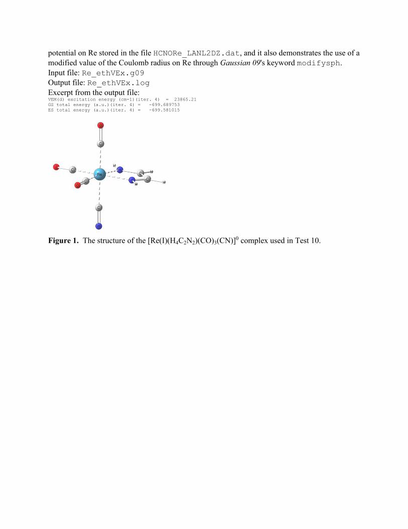
potential on Re stored in the file HCNORe_LANL2DZ.dat, and it also demonstrates the use of a

modified value of the Coulomb radius on Re through Gaussian 09's keyword modifysph.

Input file: Re_ethVEx.g09

Output file: Re_ethVEx.log




Figure 1. The structure of the [Re(I)(H4C2N2)(CO)3(CN)]0 complex used in Test 10.

18

10. Interpretation of results

If the VEMGAUSS calculation is terminated normally, the final VEM vertical excitation energy

or vertical emission energy in wavenumbers (that is, cm-1) can be found at the end of the

VEMGAUSS output file, along with the total energies of the initial and final electronic states of

the solute molecule in solution. These are the only results the user usually needs from

VEMGAUSS computations.

For the vertical excitation energy calculation the program reports the GSRF and cGSRF

excitation energies in addition to the VEM excitation energy in solution. If the ssp option is

requested, the program also reports the SMSSP solute–solvent dispersion contribution to the

gas–solvent solvatochromic shift (this contribution is not included in the VEM, GSRF, or cGSRF

energies). Here is an excerpt from the VEM excitation energy calculation for formaldehyde in

water: Symmetry of the excited state is Singlet-A2

DATA FOR EXCITATION: GS=initial_state, ES=final_state

GSRF excitation energy (cm-1)(iter. 4) = 33354.11

cGSRF excitation energy (cm-1)(iter. 4) = 33043.44

VEM(asterisk) (cm-1)(iter. 4) = 32445.05

VEM(d) excitation energy (cm-1)(iter. 4) = 32755.74



SMSSP dispersion gas-sol shift (cm-1) = 103.78

Here is an excerpt from the VEM vertical emission energy calculation for formaldehyde in

water: Symmetry of the excited state is Singlet-A2

DATA FOR EMISSION: ES=initial_state, GS=final_state

VEM(d) emission energy (cm-1) = 31012.46



The VEMGAUSS solvatochromic shift is calculated as gas − sol where gas is the gas-phase

vertical excitation energy and sol is the vertical excitation energy in solution. The vertical

excitation energy in the gas phase should be calculated at the gas-phase optimized geometry of

the solute molecule in the ground electronic state. In general, the VEMGAUSS vertical excitation

energy in solution should be calculated at the liquid-phase geometry of the solute molecule

optimized in the ground state, for example, using Gaussian 09 and the SMD implicit solvent

model. Here is an input example for the SMD ground-state geometry optimization for

formaldehyde (H2CO) in water at the M06/MG3S level of theory {the MG3S basis is described

in [Lynch, B. J.; Zhao, Y.; Truhlar, D. G. J. Phys. Chem. A. 2003, 107, 1384-1388], and for H, C,

and O [in fact for all elements from H to Ne], it is identical to 6-311+G(2df,2p)}:

%nproc=8

%mem=9000mb

# m06/6-311+G(2df,2p) opt scrf=(smd,solvent=water) int=ultrafine

GS geometry optimization of H2CO in water using SMD/M06/MG3S

0 1

8 0.0000000000 0.0000000000 0.6743110000

6 0.0000000000 0.0000000000 -0.5278530000

1 0.0000000000 0.9370330000 -1.1136860000

1 0.0000000000 -0.9370330000 -1.1136860000

To run an SMD ground-state geometry optimization, use the command g09 input (by

replacing input with the name of an actual input file).

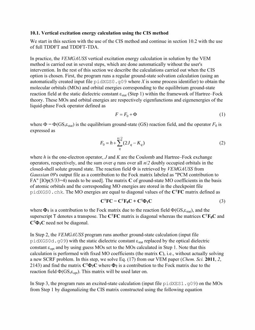
10.1. Vertical excitation energy calculation using the CIS method

We start in this section with the use of the CIS method and continue in section 10.2 with the use

of full TDDFT and TDDFT-TDA.

In practice, the VEMGAUSS vertical excitation energy calculation in solution by the VEM

method is carried out in several steps, which are done automatically without the user's

intervention. In the rest of this section we describe the calculations carried out when the CIS

option is chosen. First, the program runs a regular ground-state solvation calculation (using an

automatically created input file pidXGS0.g09 where X is some process identifier) to obtain the

molecular orbitals (MOs) and orbital energies corresponding to the equilibrium ground-state

reaction field at the static dielectric constant stat (Step 1) within the framework of Hartree–Fock

theory. These MOs and orbital energies are respectively eigenfunctions and eigenenergies of the

liquid-phase Fock operator defined as

+= 0FF (1)

where = (GS,stat) is the equilibrium ground-state (GS) reaction field, and the operator F0 is

expressed as

−+=2/

0 )2(n

q

qq KJhF (2)

where h is the one-electron operator, J and K are the Coulomb and Hartree–Fock exchange

operators, respectively, and the sum over q runs over all n/2 doubly occupied orbitals in the

closed-shell solute ground state. The reaction field is retrieved by VEMGAUSS from

Gaussian 09's output file as a contribution to the Fock matrix labeled as "PCM contribution to

FA" [IOp(5/33=4) needs to be used]. The matrix C of ground-state MO coefficients in the basis

of atomic orbitals and the corresponding MO energies are stored in the checkpoint file

pidXGS0.chk. The MO energies are equal to diagonal values of the CTFC matrix defined as

CTFC = CTF0C + CT1C (3)

where 1 is a contribution to the Fock matrix due to the reaction field (GS,stat), and the

superscript T denotes a transpose. The CTFC matrix is diagonal whereas the matrices CTF0C and

CT1C need not be diagonal.

In Step 2, the VEMGAUSS program runs another ground-state calculation (input file

pidXGS0d.g09) with the static dielectric constant stat replaced by the optical dielectric

constant opt and by using guess MOs set to the MOs calculated in Step 1. Note that this

calculation is performed with fixed MO coefficients (the matrix C), i.e., without actually solving

a new SCRF problem. In this step, we solve Eq. (17) from our VEM paper (Chem. Sci. 2011, 2,

2143) and find the matrix CT2C where 2 is a contribution to the Fock matrix due to the

reaction field (GS,opt). This matrix will be used later on.

In Step 3, the program runs an excited-state calculation (input file pidXES1.g09) on the MOs

from Step 1 by diagonalizing the CIS matrix constructed using the following equation

20

+−= ibajH iaabijjbia ||][, (4)

where the indices i and j run over all occupied MOs, the indices a and b run over all virtual MOs,

aj||ib is the antisymmetrized two-electron repulsion integral in the MO basis {see, for example,

Eq. (5) in [Maurice, Head-Gordon, Int. J. Quantum Chem.: Quantum Chem. Symp. 1995, 29,

361-370]}, and p is the energy of the molecular orbital p (p = a or i) calculated in Step 1. This

calculation gives us the CIS excitation energy and the electron density for the excited state of

interest in the ground-state reaction field approximation abbreviated as GSRF in the VEMGAUSS

output and in our VEM paper. The excited-state (ES) reaction field, (ES,opt), corresponding to

the estimated excited-state density is then evaluated by solving Eq. (19) in the VEM paper

(Chem. Sci. 2011, 2, 2143). The reaction field (ES,opt) which represents the fast (dynamic)

component of the total nonequilibrium reaction field is automatically saved in the checkpoint file

pidXES1.chk for further use.

In Step 4, the program runs a ground-state calculation (input file pidXGS1d.g09) at the fixed

MO coefficients (the matrix C) obtained in Step 1 and at the reaction field fixed at (ES,opt)

from Step 3. As in Step 2, this calculation does not solve a new SCRF problem, and its only

purpose is to obtain the CT3C matrix where 3 is a contribution to the Fock matrix due to the

reaction field (ES,opt) from Step 3.

In Step 5, we repeat the excited state calculation using a new CIS matrix constructed as

+−= ibajH iaabijjbia ||][, (5)

where the energies 'p (p = a or i) are expressed as

+= pppp || (6)

where p is the energy of the molecular orbital p obtained in Step 1. The second term of Eq. (6)

is equal to the corresponding diagonal element of the following matrix

CTC = CT3C − CT2C (7)

where 3 is a Fock matrix contribution due to the reaction field (ES,opt) from Step 3 and 2

corresponds to the reaction field (GS,opt) from Step 2. Diagonalization of the CIS matrix

constructed using Eq. (5) yields the solute's excitation energy in the nonequilibrium excited-state

reaction field expressed as (GS,stat) + (ES,opt) − (GS,opt). The corresponding excited-state

electron density is computed and used to obtained a new version of (ES,opt) while keeping

(GS,stat) and (GS,opt) unchanged. The excited-state calculation of Step 5 uses the MOs fixed

at the MOs obtained in Step 1 and the corresponding orbital energies p replaced with the new

values 'p by modifying the checkpoint file pidXGS0.chk (that comes from Step 1).

By repeating Step 4 and Step 5 we can iteratively equilibrate (ES,opt) with the excited-state

electron density for the specific excited state, thereby using a state-specific self-consistent

reaction field approach. The VEM excitation energy at the kth iteration (i.e., at the kth call of

Step 5) is defined by

−−

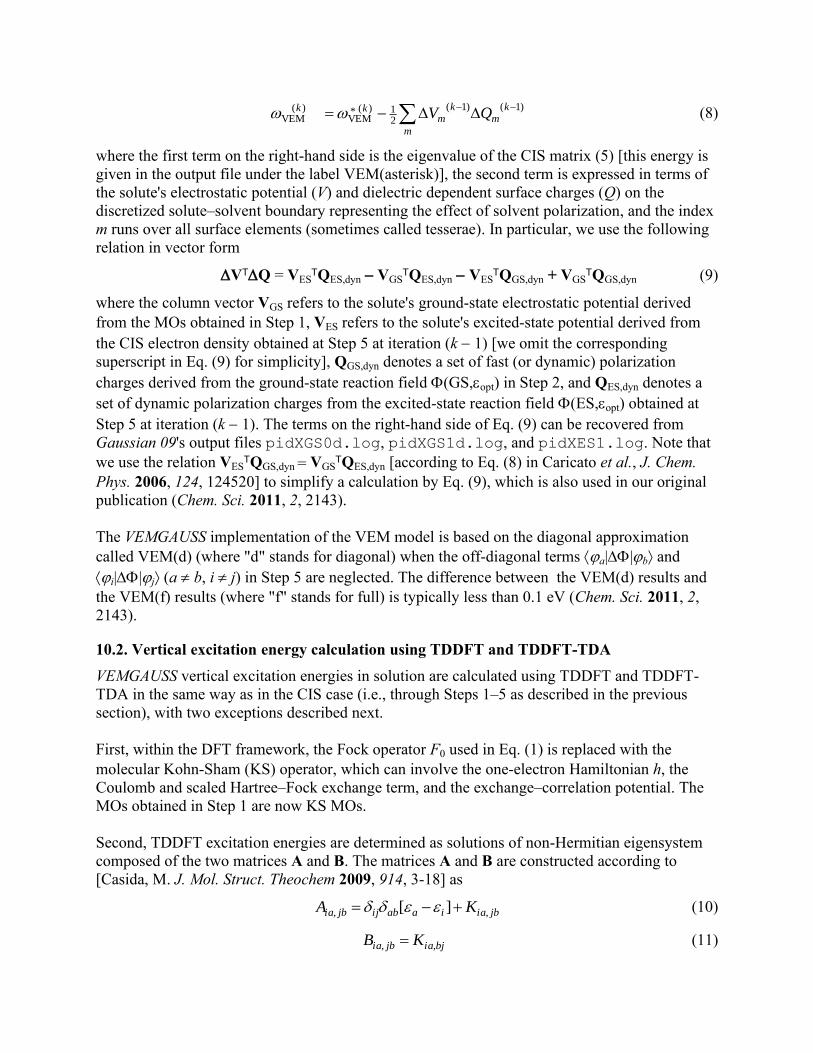
−=m

km

km

kk QV)1()1(

21)(*

VEM)(

VEM (8)

where the first term on the right-hand side is the eigenvalue of the CIS matrix (5) [this energy is

given in the output file under the label VEM(asterisk)], the second term is expressed in terms of

the solute's electrostatic potential (V) and dielectric dependent surface charges (Q) on the

discretized solute–solvent boundary representing the effect of solvent polarization, and the index

m runs over all surface elements (sometimes called tesserae). In particular, we use the following

relation in vector form

VTQ = VESTQES,dyn − VGS

TQES,dyn − VESTQGS,dyn + VGS

TQGS,dyn (9)

where the column vector VGS refers to the solute's ground-state electrostatic potential derived

from the MOs obtained in Step 1, VES refers to the solute's excited-state potential derived from

the CIS electron density obtained at Step 5 at iteration (k − 1) [we omit the corresponding

superscript in Eq. (9) for simplicity], QGS,dyn denotes a set of fast (or dynamic) polarization

charges derived from the ground-state reaction field (GS,opt) in Step 2, and QES,dyn denotes a

set of dynamic polarization charges from the excited-state reaction field (ES,opt) obtained at

Step 5 at iteration (k − 1). The terms on the right-hand side of Eq. (9) can be recovered from

Gaussian 09's output files pidXGS0d.log, pidXGS1d.log, and pidXES1.log. Note that

we use the relation VESTQGS,dyn = VGS

TQES,dyn [according to Eq. (8) in Caricato et al., J. Chem.

Phys. 2006, 124, 124520] to simplify a calculation by Eq. (9), which is also used in our original

publication (Chem. Sci. 2011, 2, 2143).

The VEMGAUSS implementation of the VEM model is based on the diagonal approximation

called VEM(d) (where "d" stands for diagonal) when the off-diagonal terms a||b and

i||j (a b, i j) in Step 5 are neglected. The difference between the VEM(d) results and

the VEM(f) results (where "f" stands for full) is typically less than 0.1 eV (Chem. Sci. 2011, 2,

2143).

10.2. Vertical excitation energy calculation using TDDFT and TDDFT-TDA

VEMGAUSS vertical excitation energies in solution are calculated using TDDFT and TDDFT-

TDA in the same way as in the CIS case (i.e., through Steps 1–5 as described in the previous

section), with two exceptions described next.

First, within the DFT framework, the Fock operator F0 used in Eq. (1) is replaced with the

molecular Kohn-Sham (KS) operator, which can involve the one-electron Hamiltonian h, the

Coulomb and scaled Hartree–Fock exchange term, and the exchange–correlation potential. The

MOs obtained in Step 1 are now KS MOs.

Second, TDDFT excitation energies are determined as solutions of non-Hermitian eigensystem

composed of the two matrices A and B. The matrices A and B are constructed according to

[Casida, M. J. Mol. Struct. Theochem 2009, 914, 3-18] as

jbiaiaabijjbia KA ,, ][ +−= (10)

bjiajbia KB ,, = (11)

22

where the quantities Kia,jb involve the matrix elements of the Hartree kernel and the exchange–

correlation kernel that depend on the KS MOs obtained in Step 1, and they do not include any

PCM terms. In Step 3, the matrix A is based on the KS orbital energies p (p = a or i) calculated

in Step 1, but in Step 5 we replace p with 'p computed according to Eq. (6).

In the case of TDDFT-TDA, the KS operator and the matrix A are constructed in the same way

as in the full TDDFT calculation but the matrix B is set to zero. The TD Hartree–Fock TDA

calculation is completely equivalent to the CIS calculation.

10.3. Note on the calculation of the relaxed density matrix

Results obtained using the current implementation of the VEM(d) method may differ slightly

from the VEM(d,RD)/PCM results cited in our original publication (Chem. Sci. 2011, 2, 2143)

because of an additional simplification in the case when the excited-state density is computed

using the Z-vector method which is Gaussian's default for TDDFT or CIS excited-state density

calculations (see http://www.gaussian.com/g_tech/g_ur/k_density.htm). In particular, the relaxed

(rel) one-particle excited-state density in solution (sol) is approximated as

ES(gas)GS(gas)unrsol

relsol →+= PPP (12)

where the first term on the right-hand side is the unrelaxed excited-state density matrix (obtained

via Gaussian 09's keyword density=RhoCI), and the second term accounts for orbital

relaxation effects due to the electronic excitation by solving the gas-phase Z-vector equation that

does not include any explicit reaction-field contributions such as the PCM term included in the

G+ matrix used in Eq. (15) by Scalmani et al., J. Chem. Phys. 2006, 124, 094107. Such

contributions were included in the original VEM/PCM formulation. However, in the current

implementation of VEM/PCM the solvation effects are still included implicitly in relaxed

excited-state density calculations because the TDDFT or CIS matrices are constructed using

solvated MOs from Step 1 and the second term of Eq. (6) from Step 5.

For background, we note that the relaxed density is explained in [Rendell, A. P. L.; Bacskay, G.

B.; Hush, N. S.; Handy, N. C. J. Chem. Phys. 1987, 87, 5976-5986].

10.4. Vertical emission energy calculation

The VEMGAUSS vertical emission energy calculation should be done in general using the

molecular geometry of the solute optimized for an excited electronic state of interest in solution.

The excited-state molecular geometry in solution can be optimized by Gaussian 09 using linear

response TDDFT calculations. Here is an example of the input file for such an optimization.

%nproc=8

%mem=9000mb

# m06/6-311+G(2df,2p) opt scrf=(smd,solvent=water) int=ultrafine td=(nstates=10,root=1)

ES geometry optimization of H2CO in water using SMD/TDM06/MG3S

0 1

8 0.0000000000 0.0000000000 0.6743110000

6 0.0000000000 0.0000000000 -0.5278530000

1 0.0000000000 0.9370330000 -1.1136860000

1 0.0000000000 -0.9370330000 -1.1136860000

To run the excited-state geometry optimization in solution, use the following command: g09 input

http://www.gaussian.com/g_tech/g_ur/k_density.htm

The VEMGAUSS vertical emission energy calculation requires the same input file as for the

VEMGAUSS vertical excitation energy calculation (except that the geometry may be different).

In the following, "em" denotes emission.

In practice, the VEMGAUSS vertical emission energy calculation is carried out in three steps that

do not require the user's intervention. In Step 1(em), the program runs a state-specific self-

consistent vertical excitation energy calculation as described in the previous paragraph, Step 1

through 5. Such a calculation is carried out in the equilibrium approximation by equating opt to

stat. The resulting excited-state reaction field, (ES,stat), is fully equilibrated with the electron

density for the excited state of interest.

In Step 2(em) (input file pidXES1em.g09), the converged reaction field (ES,stat) is

recalculated and then partitioned using the original values of opt and stat. By treating the excited

state as an initial state and the ground state as a final state, the slow portion of (ES,stat) with

respect to the final state is saved in a checkpoint file.

In Step 3(em), the program runs a nonequilibrium ground-state calculation (input file

pidXGS0em.g09) using the slow portion of the reaction field saved in Step 2(em).

10.5. Numerical examples

Scheme 1 shows results of the VEM(d,RD)/TDM06/MG3S calculations of vertical excitation

and emission energies of the acetone molecule in acetonitrile.

Scheme 1. Excitation and emission energies of the acetone molecule in acetonitrile.

State A is the equilibrium ground electronic state of the solute (acetone) molecule in solution

(from Test 7 in Section 9). State B is the first excited electronic state of the solute molecule

calculated using nonequilibrium solvation at the ground-state geometry (Test 7) when only the

fast component of the total reaction field is equilibrated with the excited-state electron density of

the solute molecule. State C is the first excited electronic state of the solute molecule calculated

using equilibrium solvation at the excited-state geometry in solution (Test 9). The B→C

relaxation step includes the full equilibration of the fast and slow degrees of freedom of the

solute–solvent system with the excited-state electron density of the solute molecule including the

solute's excited-state geometry relaxation. State D is the ground electronic state of the solute

molecule in solution calculated using nonequilibrium solvation at the solute's excited-state

geometry in solution (Test 9) when only the fast component of the total reaction field is

24

equilibrated with the solute's ground-state density. The relaxation step D→A includes the full

equilibration of the fast and slow degrees of freedom of the solute–solvent system with the

ground-state electron density of the solute molecule including the solute's ground-state geometry

relaxation.

Note that if we neglect the excited-state geometry relaxation in the step B→C by performing the

calculations of C and D at the ground-state equilibrium geometry (see Test 8), the B→C

relaxation energy will change from 3,247 to 576 cm−1, the C→D vertical emission energy will

change from 30,509 to 36,020 cm−1, and the D→A relaxation energy will change from 3,055 to

215 cm−1.

25

11. Citation of the methods used by VEMGAUSS

Publications including work performed with VEMGAUSS should cite the following:

• Marenich, A. V.; Cramer, C. J.; Truhlar, D. G.; Guido, C. A.; Mennucci, B.; Scalmani,

G.; Frisch, M. J. Practical computation of electronic excitation in solution: vertical

excitation model. Chem. Sci. 2011, 2, 2143-2161.

DOI: http://dx.doi.org/10.1039/C1SC00313E

• Marenich, A. V.; Cramer, C. J.; Truhlar, D. G. VEMGAUSS–version 2013, University of

Minnesota, Minneapolis, 2013. http://comp.chem.umn.edu/vemgauss

If the SSP option is used to include the dispersion contribution to the solvatochromic shift, the

publication should also cite

• Marenich, A. V.; Cramer, C. J.; Truhlar, D. G. Uniform treatment of solute–solvent

dispersion in the ground and excited electronic states of the solute based on a solvation

model with state-specific polarizability. J. Chem. Theory Comput. 2013, 9, 3649-3659.

DOI: http://dx.doi.org/10.1021/ct400329u

Users of the Gaussian 09 code should follow the instructions in their Gaussian 09 license for

citing the Gaussian 09 code.

http://dx.doi.org/10.1039/C1SC00313E

http://comp.chem.umn.edu/vemgauss

http://dx.doi.org/10.1021/ct400329u

26

12. Computers and operating systems on which VEMGAUSS has been tested

The VEMGAUSS program has been tested using the following specifications:

• HP Linux cluster with 1,091 HP ProLiant BL280c G6 blade servers, each with two-

socket, quad-core 2.8 GHz Intel "Nehalem" processors; with gfortran gcc version gcc-4.4.7

[CentOS release 6.4 (Final)]

• SGI Altix XE 1300 Linux cluster with 180 SGI Altix XE 300 compute nodes, each

containing two quad-core 2.66 GHz Intel Xeon "Clovertown"-class processors; with gfortran

gcc version gcc-4.4.6 [CentOS release 6.3 (Final)]

• SGI Altix UV 1000 Linux cluster with 1,140 compute cores (190 6-core Intel Xeon X7542

"Westmere” processors at 2.66 GHz); with gfortran gcc version gcc-4.4.3 [SUSE Linux

Enterprise Server 11 SP2 (x86_64)]

27

13. Revision history

Version 2013

Version 2013 is the first distributed version.

Documents

VEMGAUSS - Chemical Theory Center