Vehicular Cloud: Stochastic Analysis of Computing ... Cloud: Stochastic Analysis of Computing Resources in a Road Segment by TaoZhang Thesis submitted to the Faculty of Graduate and

Vehicular Cloud: Stochastic Analysis of

Computing Resources in a Road Segment

by

Tao Zhang

Thesis submitted to the

Faculty of Graduate and Postdoctoral Studies

In partial fulfillment of the requirements

For the M.A.Sc. degree in

Electrical and Computer Engineering

School of Electrical Engineering and Computer Science

Faculty of Engineering

University of Ottawa

c© Tao Zhang, Ottawa, Canada, 2016

Abstract

Intelligent transportation systems aim to provide innovative applications and services

relating to traffic management and enable ease of access to information for various system

users. The intent to utilize the excessive on-board resources in the transportation system,

along with the latest computing resource management technology in conventional clouds,

has cultivated the concept of the Vehicular Cloud. Evolved from Vehicular Networks, the

vehicular cloud can be formed by vehicles autonomously, and provides a large number

of applications and services that can benefit the entire transportation system, as well as

drivers, passengers, and pedestrians. However, due to high traffic mobility, the vehicular

cloud is built on dynamic physical resources; as a result, it experiences several inherent

challenges, which increase the complexity of its implementations.

Having a detailed picture of the number of vehicles, as well as their time of availability

in a given region through a model, works as a critical stepping stone for enabling vehicular

clouds, as well as any other system involving vehicles moving over the traffic network.

The number of vehicles represents the amount of computation capabilities available in

this region and the navigation time indicates the period of validity for a specific compute

node. Therefore, in this thesis, we carry out a comprehensive stochastic analysis of

several traffic characteristics related to the implementation of vehicular cloud inside a

road segment by adopting proper traffic models. According to the analytical results, we

demonstrate the feasibility of running a certain class of applications or services on the

vehicular cloud, even for highly dynamic scenarios.

Specifically, two kinds of traffic scenarios are modeled: free-flow traffic and queueing-

up traffic. We use a macroscopic traffic model to investigate the free-flow traffic and

analyze the features such as traffic density, the number of vehicles and their residence

time. Also, we utilize the queueing theory to model the queueing-up traffic; the queue

length and the waiting time in the queue are analyzed. The results show the boundaries

on enabling vehicular cloud, allowing to determine a range of parameters for simulating

vehicular clouds.

ii

Acknowledgements

I will be ever grateful to a number of sincere people who have guided and motivated me

throughout my thesis work. I express my deepest appreciation to my supervisor Professor

Azzedine Boukerche, who continually conveyed a spirit of adventure in research. I would

like to thank him for giving me the chance to study in PARADISE Research Laboratory,

supporting me to research and giving me critical and insightful feedbacks to my work.

I would like to thank Dr. Robson E. De Grande who has been a tremendous mentor

for me. His guidance and advice helped me all the time during my research. I also

appreciate his patience in settling all my doubts at the beginning of this wonderful

journey. His advice on both research as well as on my life has been priceless. Without

his patience, motivation, enthusiasm, and immense knowledge, this dissertation would

not be possible.

In addition, my special thanks go to my colleagues at PARADISE Research Labo-

ratory for all the fun times and collaboration. It was my great pleasure to know all of

them. I will cherish the memory of the times we spend together.

Finally, I thank my dear parents, sister and girlfriend for their encouragement and

love that kept my morale high throughout the ups and downs during my research.

iii

Publications Related to Thesis

Tao Zhang, Robson E. De Grande, and Azzedine Boukerche. 2015. Vehicular

Cloud: Stochastic Analysis of Computing Resources in a Road Segment. In Proceed-

ings of the 12th ACM Symposium on Performance Evaluation of Wireless Ad Hoc,

Sensor, & Ubiquitous Networks (PE-WASUN ’15). ACM, New York, NY, USA, 9-16.

DOI=http://dx.doi.org/10.1145/2810379.2810383

Tao Zhang, Robson E. De Grande, and Azzedine Boukerche. ”Urban Traffic Charac-

terization for Enabling Vehicular Clouds” in Wireless Communications and Networking

Conference (WCNC), 2016 IEEE (Accepted).

Tao Zhang, Robson E. De Grande, and Azzedine Boukerche. ”Analyzing Traffic Flows

through Stochastic Models for Vehicular Clouds.” Ad Hoc Networks (2016) (Submitted).

iv

Contents

1 Introduction 1

1.1 Background . . . . . . . . . . . . . . . . . . . . . . . . . . . . . . . . . . 2

1.2 Problem Statement . . . . . . . . . . . . . . . . . . . . . . . . . . . . . . 3

1.3 Contribution . . . . . . . . . . . . . . . . . . . . . . . . . . . . . . . . . . 4

1.4 Thesis Organization . . . . . . . . . . . . . . . . . . . . . . . . . . . . . . 6

2 Related Work 8

2.1 Vehicular Network . . . . . . . . . . . . . . . . . . . . . . . . . . . . . . 10

2.1.1 Architecture of VANET . . . . . . . . . . . . . . . . . . . . . . . 10

2.1.2 Comparison of VANET and MANET . . . . . . . . . . . . . . . . 12

2.1.3 VANET Applications . . . . . . . . . . . . . . . . . . . . . . . . . 14

2.2 Cloud Computing . . . . . . . . . . . . . . . . . . . . . . . . . . . . . . . 14

2.2.1 IaaS: Infrastructure as a Service . . . . . . . . . . . . . . . . . . . 16

2.2.2 PaaS: Platform as a Service . . . . . . . . . . . . . . . . . . . . . 16

2.2.3 SaaS: Software as a Service . . . . . . . . . . . . . . . . . . . . . 17

2.3 Mobile Cloud Computing . . . . . . . . . . . . . . . . . . . . . . . . . . . 17

2.4 Vehicular Cloud Computing . . . . . . . . . . . . . . . . . . . . . . . . . 20

2.4.1 Taxonomy of Literature on VCC . . . . . . . . . . . . . . . . . . 22

2.4.2 Architecture of Vehicular Cloud . . . . . . . . . . . . . . . . . . . 24

vi

2.4.3 Vehicular Cloud Services . . . . . . . . . . . . . . . . . . . . . . . 27

2.4.4 Applications of Vehicular Cloud . . . . . . . . . . . . . . . . . . . 29

2.5 Mathematical Modeling of Vehicular Cloud . . . . . . . . . . . . . . . . . 35

2.5.1 Car-Following Models . . . . . . . . . . . . . . . . . . . . . . . . . 35

2.5.2 Traffic Stream Models . . . . . . . . . . . . . . . . . . . . . . . . 36

2.5.3 Stochastic Traffic Models . . . . . . . . . . . . . . . . . . . . . . . 38

2.6 Summary . . . . . . . . . . . . . . . . . . . . . . . . . . . . . . . . . . . 38

3 Stochastic Modeling 41

3.1 Free-flow Model . . . . . . . . . . . . . . . . . . . . . . . . . . . . . . . . 41

3.2 Queueing-up Model . . . . . . . . . . . . . . . . . . . . . . . . . . . . . . 47

4 Analytical Results 53

4.1 Free-flow Model . . . . . . . . . . . . . . . . . . . . . . . . . . . . . . . . 54

4.1.1 Traffic Load . . . . . . . . . . . . . . . . . . . . . . . . . . . . . . 54

4.1.2 Residence Time . . . . . . . . . . . . . . . . . . . . . . . . . . . . 58

4.2 Queuing-up Model . . . . . . . . . . . . . . . . . . . . . . . . . . . . . . 58

4.2.1 Traffic Load . . . . . . . . . . . . . . . . . . . . . . . . . . . . . . 59

4.2.2 Residence Time . . . . . . . . . . . . . . . . . . . . . . . . . . . . 63

5 Conclusion and Future Work 66

5.1 Conclusion . . . . . . . . . . . . . . . . . . . . . . . . . . . . . . . . . . . 66

5.2 Future Work . . . . . . . . . . . . . . . . . . . . . . . . . . . . . . . . . . 67

A Glossary of Terms 68

vii

List of Tables

2.1 Comparison of CC, MCC and VCC . . . . . . . . . . . . . . . . . . . . . 20

2.2 Representative Works on Vehicular Cloud Applications–Part1 . . . . . . 30





2.7 Strengths and Weaknesses of Existing Traffic Models . . . . . . . . . . . 39

4.1 Summary of Experimental Parameters . . . . . . . . . . . . . . . . . . . 53

viii

List of Figures

1.1 Vehicular Clouds . . . . . . . . . . . . . . . . . . . . . . . . . . . . . . . 3

1.2 Vehicular Cloud Resource Management Layers . . . . . . . . . . . . . . . 5

1.3 Traffic conditidons under the flow of vehicles in road segment . . . . . . . 5

2.1 Technologies Contributing Towards Vehicular Cloud Computing . . . . . 9

2.2 Architecture of VANET . . . . . . . . . . . . . . . . . . . . . . . . . . . 12

2.3 Architecture of Amazon EC2 . . . . . . . . . . . . . . . . . . . . . . . . . 16

2.4 Taxonomy of the Literature on Vehicular Cloud Computing . . . . . . . . 22

2.5 Vehicular Cloud Computing Architecture . . . . . . . . . . . . . . . . . . 25

3.1 Free-flow Traffic in Roadway Segment [SD] . . . . . . . . . . . . . . . . . 42

3.2 Occurrence . . . . . . . . . . . . . . . . . . . . . . . . . . . . . . . . . . 44

3.3 Exceedance . . . . . . . . . . . . . . . . . . . . . . . . . . . . . . . . . . 44

3.4 A illustration of a queue in a road segment . . . . . . . . . . . . . . . . . 48

4.1 Average Number of Vehicles versus Vehicular Density over [SD] . . . . . 54

4.2 Average Number of Vehicles versus Road Length of [SD] . . . . . . . . . 55

4.3 Average Number of Vehicles versus Max Speed Limit within [SD] . . . . 56

4.4 The Probablity P [N(t)] . . . . . . . . . . . . . . . . . . . . . . . . . . . 57

4.5 Number of Vehicles Distribution versus Vehicular Density . . . . . . . . 58

ix

4.6 Average Residence Time versus Max Speed Limit within [SD] . . . . . . 59

4.7 Mean Number of Vehicles in a Roadway Segment versus Traffic Intensity 60

4.8 Probability Mass Function . . . . . . . . . . . . . . . . . . . . . . . . . . 61

4.9 Number of Vehicles with Exponential Leaving Time . . . . . . . . . . . . 61

4.10 Probability Mass Function . . . . . . . . . . . . . . . . . . . . . . . . . . 62

4.11 Number of Vehicles with Fixed Leaving Time . . . . . . . . . . . . . . . 62

4.12 Mean Waiting Time in the Queue Arrival Rate . . . . . . . . . . . . . . . 63

4.13 PDF of Waiting Time in the Queue with Exponential Leaving Time . . . 64

4.14 Pr[W(w)> t] with Exponential Leaving Time . . . . . . . . . . . . . . . 64

4.15 PDF of Waiting Time in the Queue with Fixed Leaving Time . . . . . . 65

4.16 Pr[W(w)>t] with Fixed Leaving Time . . . . . . . . . . . . . . . . . . . 65

x

Chapter 1

Introduction

Due to the advent of cloud computing and the maturity of its technology, various users

are able to access services at any point in time and space. The emergence of a new type of

cloud–the vehicular cloud–has been a prominent step forward for intelligent transporta-

tion systems. The vehicular cloud is formed autonomously by the traffic on the road,

and each vehicle serves as a compute node for the cloud, which offers a great number

of benefits not only to drivers, passengers, and pedestrians but also to the municipal

traffic manager and city planners. Those self-organized clouds can work independently,

as well as complementing to the conventional cloud structure and providing processing

power to deal with the traffic-related issues. This trend is quite promising, due to the

sky-high increase in the rate of the number of vehicles on the road. According to US

National Transportation Statistics [95], the number of vehicles in American roadways,

has reached 253.6 million. Harnessing the excessive computing power of those vehicles

has a profound significance for information technology (IT), the economy and society.

1

2

1.1 Background

Thanks to the revolutionary change in the automotive industry, an increasing number

of ”smart vehicles” are introduced to drivers for daily use. A typical vehicle today is

regarded as a ”computer-on-wheels” due to the reason that it is likely to equip with a pow-

erful on-board computer, a large capacity storage device, a sensitive radio transceiver,

a rear collision radar and a GPS device. Meanwhile, rapid technological advances in

cloud computing [77] provide sufficient technical support for building a dynamic cloud

in mobile environments. Cloud can provision resources and services on-demand over the

Internet, just like a public utility [52]. Amazon Elastic Compute Cloud (Amazon EC2)

is now the largest online retailer to provide dynamic compute capacity in the cloud. On

the other hand, an increasing number of businesses prefer to rent their servers, platforms

or software in an elastic and scalable manner, instead of purchasing and maintaining

them by themselves [10]. The reciprocal benefit accelerates the prosperity of cloud com-

puting, whose main features include pay-as-you-go, virtualization technology, resources

on demand, scalability and Quality of Service (QoS). As a result, cloud computing is

becoming the main technological trend in IT, and enterprises nowadays invest massive

effort in migrating their services to the cloud.

Motivated by the above-mentioned facts and opportunities, the vehicular cloud frame-

work was initially proposed in [79]. In general, various underutilized vehicular resources

such as computing power, network connectivity, sensing capability, and storage can be

shared with car owners. Moreover, the aggregated resources can be rented to potential

consumers following a specific business model, similar to the traditional cloud infrastruc-

ture.

Figure 1.1 shows two types of vehicular cloudlet, which is defined as a group of ve-

hicles can share resources with each other via vehicle to vehicle (V2V) communication

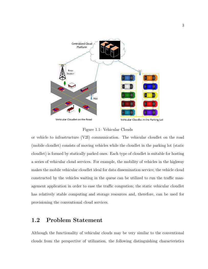
3

Figure 1.1: Vehicular Clouds

or vehicle to infrastructure (V2I) communication. The vehicular cloudlet on the road

(mobile cloudlet) consists of moving vehicles while the cloudlet in the parking lot (static

cloudlet) is formed by statically parked ones. Each type of cloudlet is suitable for hosting

a series of vehicular cloud services. For example, the mobility of vehicles in the highway

makes the mobile vehicular cloudlet ideal for data dissemination service; the vehicle cloud

constructed by the vehicles waiting in the queue can be utilized to run the traffic man-

agement application in order to ease the traffic congestion; the static vehicular cloudlet

has relatively stable computing and storage resources and, therefore, can be used for

provisioning the conventional cloud services.

1.2 Problem Statement

Although the functionality of vehicular clouds may be very similar to the conventional

clouds from the perspective of utilization, the following distinguishing characteristics

4

make it unique and not easy to deal with.

• The most challenging aspect of building vehicular cloud is dealing with the highly

dynamic availability of the vehicles, which distinguishes the vehicular cloud ar-

chitecture from traditional cloud models. The autonomous cooperation among

vehicles and their “decentralized” management contribute to the complexity and

uniqueness of the vehicular cloud.

• Accurately determining the amount of vehicles and their available time frame is crit-

ical for constructing a vehicular cloud. The analysis of the availability of resources

in this particular scenario is totally and directly involved with the perception of

the traffic flow for a given area, such as a road segment, during a time span. Nev-

ertheless, the number of vehicles varies continually, since the same vehicles move

dynamically, with diverse traveling times, behaviors, and speeds.

• Since the vehicular clouds are not as stable as the conventional clouds, the resource

management system (see Fig 1.2) of vehicular cloud should be able to the predict

the amount the available computing capabilities, and the task scheduling system

needs to schedule the computation tasks on the dynamic resources for the sake of

providing consistent service to the authorized customers.

1.3 Contribution

The main contribution of this thesis is a detailed stochastic analysis about the distribu-

tion of the vehicles and their available time range within a road segment in an urban

area. Two specific traffic scenarios are considered – free flow traffic and queueing-up

traffic, as depicted in Figure 1.3. These two scenarios are very common traffic situations

nowadays in the urban roadways of metropolitan cities.

5

Base Station RSU Vehicle

Physical Resources

Dynamic Resource Manager

Computing Task Scheduler

Resource Virtualization Agent

Resource Controller

Northbound API

Applications

Figure 1.2: Vehicular Cloud Resource Management Layers

Figure 1.3: Traffic conditidons under the flow of vehicles in road segment

6

This is a preliminary step towards utilizing excessive vehicular resources and con-

structing the vehicular cloud in a highly dynamic environment. Specifically,

• To analyze the specific features and characteristics of vehicular cloud, we study

and classify the existing related works of VANETs, cloud computing and vehicular

cloud. Comparison of these technologies reflects the evolution of the concept of

vehicular cloud. The information is presented and summarized in an appropriate

way.

• A macroscopic model in [60] is utilized as a base to analyze the features of free-flow

traffic in a roadway segment. We first obtain the average number of vehicles, then

we get the distribution of the number of vehicles inside the road segment.

• We use the queue theory to model the queueing-up traffic. The analytical form

of the length of the traffic queue and the waiting time of vehicles are presented.

Those two features are important for the reason that they represent the amount of

available computation resource and their valid time, respectively.

• Based on the models, we carry out the comprehensive analysis of several traffic

characteristics related to the implementation of vehicular clouds for both traffic

scenarios.

1.4 Thesis Organization

The remainder of this thesis is organized as follows:

• Chapter 2 surveys the state-of-the-art technology of vehicular cloud computing.

We highlight Vehicular Cloud, an extension of traditional Cloud Computing with

many inherent new features. In addition, we present a comparative study between

7

cloud computing and vehicular cloud computing as well as explaining the vehicu-

lar cloud computing architecture, autonomous cloud formation, and the potential

applications.

• Chapter 3 provides the mathematical modeling of the study. This chapter is com-

posed of two sections; the first focuses on the free-flow traffic scenario and the

second works on the queueing-up traffic scenario.

• Chapter 4 demonstrates the analytical results, and presents the detailed analysis

of each scenario.

• Chapter 5 concludes the results and describes our future directions of research.

Chapter 2

Related Work

Evolved from Vehicular Ad-Hoc Network (VANET), presently, vehicular cloud comput-

ing (VCC) has received much attention. VCC is an attractive technology, which takes

advantage of cloud computing to support many novel applications. Therefore, the ob-

jectives of VCC are to offer various computational services at low cost to the authorized

users, to ease traffic congestion and to improve road safety. In this chapter, we pro-

vide a survey of VCC and our aim is to help readers better understand the fundamental

vehicular cloud computing mechanisms.

The flow chart 2.1 classifies existing techniques that are contributing towards the

generation of vehicular cloud computing, which can be seen as a combination of two

technical paradigms i.e., ad hoc network and cloud computing.

All nodes in wireless ad hoc networks can be dynamically connected in an arbitrary

manner. As the transmission range of each node is limited and different [29] [28], the

sender may need the aid of its neighboring nodes to forward the packets to the receiver.

Since wireless ad hoc networks do not rely on pre-installed static infrastructure for com-

munication, the localization of the nodes becomes one of the major issues [17] [36] [21]

[80] [18] [14], especially in MANETs where the nodes are mobile. All nodes in the ad

8

Related Work 9

hoc networks behave as routers, which discover and maintain the routes to the next hop

in the network. Therefore, the routing protocols are vital for enhancing the efficiency

and reliability of the dissemination of packets [98] [26] [31] [25] [19]. Other challenges of

ad hoc network include security [15] and energy consumption [91] [30]. Compared to the

traditional ad hoc networks, mobile ad hoc networks (MANET) are more dynamic since

the nodes are not fixed [22] [23] and the Vehicular Ad-hoc Network (VANET) primarily

adapts from Mobile Ad hoc Networks (MANETs) [24] [88] where the communication

among the nodes is generally single hop or multi-hop based.

On the other side, distributed computing and grid computing [6] [27] [16] have enor-

mously contributed to the emergence and prosperity of cloud computing; and the concept

of VCC originates from Mobile Cloud Computing (MCC) where the main concern is to

access traditional cloud services provided by Infrastructural-Cloud in a way similar to

access telecommunication and other data based services.

Ad hoc Networks Cloud Computing

Mobile Adhoc Networks (MANET)

Mobile Cloud Computing (MCC)

Vehicular Adhoc Networks (VANETs)

Vehicular CloudComputing(VCC)

Figure 2.1: Technologies Contributing Towards Vehicular Cloud Computing

Related Work 10

2.1 Vehicular Network

Traffic congestion in the urban area is a daily event, the growth in the number of vehicles

on the road has put huge stress on transportation systems and this tremendous growth

of vehicles has lead to unsafe and unpleasant driving experience. Most of the time, we

are not alerted by beforehand notification of congestion. Thus, existing transportation

infrastructure requires improvements in traffic safety and efficiency. The municipal traffic

management department has planned various solutions such as expanding lanes on high-

ways and reducing the number of stop signs and traffic lights to reduce traffic congestion.

However, those solutions are ineffective and may even increase congestion and pollution

levels. The cutting edge technological advancements have been considered to enable such

diverse traffic applications as traffic hazard detection, cooperative traffic monitoring, and

control of traffic flow. Inspired by Mobile Ad-hoc Networks [68], a new kind of network,

which incorporate Vehicle to Vehicle (V2V) and Vehicle to Infrastructure (V2I) commu-

nication, is named as Vehicular Ad Hoc Network (VANET), which has been considered

as an excellent network environment for Intelligent Transportation System (ITS).

2.1.1 Architecture of VANET

Figure 2.2 shows the architecture of VANET. The V2V and V2I communication are

achieved through a device called Wireless Access in Vehicular Environment (WAVE).

Specifically,

• V2V are communications between vehicles in ad hoc mode [58]. A vehicle can

transmit or receive useful traffic-related messages such as traffic accidents and road

conditions to/from other vehicles.

• V2I is used for the valuable information exchange between vehicles and fixed net-

Related Work 11

work infrastructure [58]. In this mode, a vehicle could communicate with external

networks such as the Internet by utilizing RSU as a gateway. V2I links are more

secure and require more bandwidth than V2V links.

In addition, the 5.9 GHz frequency spectrum band has been allocated for Short Range

Communication (DSRC) between vehicles [7]. The main components of the architecture

are on-board units (OBUs), road side units (RSUs) and certification authorities (CAs).

• OBU, along with a set of sensors, resides in each vehicle and it collects the infor-

mation of the vehicle and transmits information such as the position, speed and

acceleration/deceleration to other vehicles or RSUs through the wireless medium.

At the same time, OBU also receives the messages from other sources and has the

ability to verify the incoming message and avoid security attacks.

• RSU is a physical communication equipment at a fixed location and responsible

for collecting and disseminating traffic-related information such as the length of

the traffic queue, accident spot ahead and nearest parking lots and gas stations.

RSU is equipped with at least one network device for the Internet and short-range

wireless communication. RSU acts as a gateway for the OBU to access the Internet,

which also enables vehicles within the communication range to establish Internet

connections. RSU can be deployed along the road to monitor the traffic flow or in

the road intersections to offer help in coordinating the traffic lights and collecting

information about vehicle activities.

• To prevent the possible security problems in VANETs [74], CA has the information

of all vehicles in order to verify that the source of the message is a valid entity.

It is vital for the performance of VANET and should be a fully trusted party; for

instance, the municipal transportation department could play the role as a CA.

Related Work 12

RSU

V2I

RSU

RSU

OBU

OBU

2V

V2I

InternetCA

Figure 2.2: Architecture of VANET

2.1.2 Comparison of VANET and MANET

VANET is evolved from MANET and it is a subclass of MANET [85]. From MANET

perspective, the ad-hoc domain is composed by RSU and OBU, which are considered as

the static (fixed) node and the mobile node, respectively. Moreover, they are both based

on IEEE 802.11p protocol.

• In the ad-hoc network, every wireless transmission has distance coverage limita-

tion, wireless node will use its neighboring nodes to forward the packet beyond its

coverage [111]. To improve the reliability, MANET nodes require ad-hoc types rout-

ing protocols such as table-driven routing, on-demand routing, and hybrid routing

[112]. The routing protocols of MANET can not simply apply to VANET network

as MANET has fast changing ad-hoc network topology.

• The size of VANET is much larger than that of MANET. Each vehicle represents a

valid mobile node in VANET and there are a considerable number of vehicles within

an area, especially in the urban area. Therefore, we normally divide VANET into

Related Work 13

small pieces and design protocols and applications which are fit for local traffic

situation. At the same time, those partitions of VANET are able to communicate

with each other via the stationary RSU.

• The topology of VANET is more or less determined by the layout of the roads

and the traffic conditions. The mobile nodes cannot move around arbitrarily as

in MANET and their possible routes are restricted within the roadway segment.

Therefore, the position of the mobile node in VANET is more predictable than that

in MANET.

• When it comes to designing MANET, we should pay the utmost attention to the

power consumption of each node. Usually, we need to compromise the system

throughput due to node’s power capacity, which actually becomes a bottleneck for

the entire MANET system. Contrarily, VANET nodes (OBU) are not subject to

storage and power limitation because they reside in vehicles, which provides enough

power to support all the tasks in OBU.

• Without the power limitation, the computation system of OBU can be more so-

phisticated and more complex computation tasks can be assigned to this VANET

distributed system.

• Since vehicles are fast-moving on the road, the nodes in VANET are highly mo-

bile and the network topology changes constantly. As a result, the VANETs are

ephemeral networks [86] and this is the most significant difference between VANET

and MANET. The node distribution density highly depends on the traffic. Typi-

cally it is lower during the night time and much higher during the rush hours. It is

apparent that vehicles’ navigation speeds and directions are unpredictable, there-

fore, sometimes the connection time between two vehicles could be very short. It

Related Work 14

needs to be considered when designing the protocols [2] and algorithms in order to

increase the reliability [4] and decrease the packet dropping probability.

2.1.3 VANET Applications

The main VANET applications can be categorized into three classes [76] [74] [96]:

• Applications for road safety. VANET applications provide valuable messages [20]

such as collision avoidance, notification danger of the road and warnings of harsh

weather for the sake of improving road safety and reducing traffic accidents.

• Applications for traffic efficiency. These applications aim to help drivers make

better use of the road and assist the driver in certain situations such as overtaking

vehicles, warning of potential traffic jams, detection of vehicle queue, etc.

• Applications of passengers comfort. They are value added applications and for the

comfort of the driver and passengers with on-board services such as infotainment,

messaging, Internet access, etc.

2.2 Cloud Computing

Thanks to the revolutionary change of computation and networking technologies, the past

few years have witnessed the tremendous advancement of Cloud Computing (CC)[62][12][40],

which is a paradigm shift in information technology (IT) industry all over the world.

Based on [75], CC is defined as ”cloud computing is a model for enabling ubiquitous,

convenient, on-demand network access to a shared pool of configurable computing re-

sources (e.g., networks, servers, storage, applications and services) that can be rapidly

provisioned and released with minimal management effort or service provider interac-

tion.” Compared to the traditional local systems, CC has several novel characteristics:

Related Work 15

• It provides computational resources, storage, and IT services on demand. From

user’s perspective, it has infinite computing resources available; thus, they don’t

need to plan ahead for physical resource provisioning.

• Various users may rent the amount of services they need at the moment. CC allows

them to purchase extra hardware resources only when there is an increase in their

needs. It is really helpful for the start-ups as they don’t need to set up big financial

commitments for building up the IT infrastructure in advance.

• CC also gives users the ability to rent computing resources in a short period of

time as needed. For example, the users can rent the resources based on the length

of a project; after the completion the project, they can release them. It will be a

huge waste of money if they buy their own physical servers for the project instead

of renting them from CC.

An increasing number of individual users and enterprises have migrated their data and

IT services to remote cloud servers. Amazon elastic computing cloud (EC2) is the one

of the largest cloud services platform, which has attracted millions of users all over the

world.

Figure 2.3 illustrates the EC2 architecture [41]. An authorized user can access the

cloud services by the client web API and EC2 platform can provide the elastic computing

resources (EC2 instances) and storage (Elastic Block Storage and Ephemeral Storage).

Cloud Watch monitors the resource usage of the customers and reports the results to Auto

Scaling system, which is a decision-maker and has the ability to scale up or scale down

the quota of resources for the users. Essentially, there are three types of technologically

mature cloud services [62][66]. Namely, Infrastructure as a Service (IaaS), Platform as a

Service (PaaS) and Software as a Service (SaaS).

Related Work 16

Client Web API

Load Balancer

Security Groups

AmazonMachineImage

Figure 2.3: Architecture of Amazon EC2

2.2.1 IaaS: Infrastructure as a Service

Based on virtualization technology, the cloud service provider offers its customers elastic

resources such as computing capabilities, network connections, and storage capacity [45].

Amazon EC2 [8] is a very good example of this category. For the open-source project,

OpenStack is one of the most popular software platforms for cloud computing, mostly

deployed as an infrastructure-as-a-service [102]. There are several interrelated compo-

nents in this software platform. For instance, Nova controls hardware pools of processing;

Neutron deals with networking resources, Cinder manages block storage and Swift ad-

ministers the object storage. Users either manage it through a web-based dashboard

(Horizon), through command-line tools, or through a RESTful API.

2.2.2 PaaS: Platform as a Service

PaaS provides a platform where applications can be developed, run and managed by

authorized users without worrying about some of the lower-level details of the environ-

ment. In other words, the consumer have the control over configuration settings and

Related Work 17

software deployment, and the service provider offers the servers, the networks, storage

and other services to host the consumer’s application. Microsoft Azure [104] and Google

AppEngine [109] are typical service platforms of this category.

2.2.3 SaaS: Software as a Service

In SaaS model, software resides in the service provider’s datacenter and is maintained

by the provider [70], who licenses various applications, including office and messaging

software, database management system (DBMS) software, CAD software, customer re-

lationship management (CRM) software, antivirus, etc., to customers as a service on

demand. SaaS is subscription based, this allows customers to rent rather than purchase

the software. In addition, there is no need for customers to worry about the compatibility

between the software and their operating system since the user can access the service

simply by launching their browsers and log on during the terms of the subscription. IBM

SmartCloud [54] platform is an example of SaaS model.

2.3 Mobile Cloud Computing

The popularity and portability of mobile devices such as tablets, PDAs and smartphones

have brought a new research area called Mobile Cloud Computing (MCC) [92][37], where

the mobile devices normally provide the input and the computation tasks are performed

by the virtual machines on a remote cloud server. The MCC forum defines MCC as

follows [72]: ”Mobile cloud computing at its simplest refers to an infrastructure where

both the data storage and data processing happen outside of the mobile device. Mobile

cloud applications move the computing power and data storage away from mobile phones

and into the cloud, bringing applications and mobile computing to not just smartphone

Related Work 18

users but a much broader range of mobile subscribers” MCC is known to be a promising

technology in the IT arena due to its incomparable features such as mobility, portability,

and communication. Several features are unique in MCC [37]:

• Prolonging battery lifetime. One of the main concerns for mobile devices is the

battery life. Short battery life means the user has to charge them more frequently,

which is definitely a weak point of those electronic products. Many methods have

been proposed to tackle this issue by enhancing CPU performance and managing

the screen and disk in an intelligent manner to lower down their power consumption.

However, those solutions are expensive due to the requirements of the fundamental

change in the structure of mobile devices, such as a new circuit layout design or an

upgraded hardware. It may not be practicable for all mobile devices, especially for

products which are already in customers’ hand. In MCC, computation offloading

technique is utilized to migrate the heavy computation tasks and complex process-

ing from mobile devices to remote servers in the cloud. It will significantly reduce

the application execution time on mobile devices and, consequently, extend the

battery life.

• Improving processing capability and storage capacity. MCC is able to reduce the

running cost for compute-intensive applications in terms of time and energy con-

sumption. It is obvious that each mobile device has limited physical resources such

as processing power and storage capacity. MCC can efficiently support heavy and

complex applications on portable mobile devices since it enables mobile users to

run the computation tasks online and store the large data on the cloud through

wireless networks.

• Improving reliability. MCC can effectively improve the reliability of mobile devices

by running applications or storing data on clouds because the data and processing

Related Work 19

results are stored and backed up on remote servers. This feature can greatly reduce

the risk of data and application loss on the mobile devices. In addition, different

data security models can be applied in MCC to provide stronger data protection for

both service providers and users. For example, cloud-based mobile digital rights

management (DRM) schemes can be used to protect mass of unstructured digi-

tal contents (e.g., video, audio, and music) from being pirated and unauthorized

distribution [114].

Moreover, MCC also inherits some advantages of CC for mobile services as follows

[75] [37]:

• Dynamic provisioning. MCC provides authorized users the facility of unlimited

resources on a fine-grained, self-service basis. This enables service providers and

mobile users to run their applications without early planning of resource provision-

ing. In addition, the flexible resource provisioning also permits service providers

to deploy their mobile applications on a minimum amount of resources at the

beginning and scale up their hardware resources based on the popularity of the

applications.

• Ease of access. Mobile application services can be accessed from anywhere in the

world and the users are capable of accessing the resources at any time as long as

they have internet access on the mobile devices.

• Ease of integration. By resource pooling, service providers can share resources and

costs to support a multitude of applications and meet the user demand.

Related Work 20

2.4 Vehicular Cloud Computing

The concept of vehicular cloud has been first proposed in recent works [3] [79] [78]. The

key point of vehicular cloud comprehends the collection, utilization, and allocation of

the excessive on-board resources, such as computing capabilities, sensors, storage, and

communication resources, in a dynamic group of vehicles under the authorization of the

vehicle owners. Combining such resources together and enabling them to provide cloud

services to the public benefit both the cloud and owner of vehicles. The services that

vehicular clouds can offer are non-trivial and complementary to the conventional cloud

computing. According to the proposal in [78], VC refers to a group of largely autonomous

vehicles whose corporate computing, sensing, communication, and physical resources can

be coordinated and dynamically allocated to authorized users. Table 2.1 compares the

features of CC, MCC, and VCC from different perspectives.

Table 2.1: Comparison of CC, MCC and VCCFeature Cloud

Computing

Mobile Cloud

Computing

Vehicular Cloud

Computing

ComputationCapability

Highest Lowest Medium sized

Supports MobileResources

No Yes Yes

Storage Capacity Highest Lowest Medium sizedBatteryLimitation

No Yes No

PhysicalResources

Local or RemoteServers

Local Mobile De-vices or RemoteServer

Local Vehicles orRemote Servers

NetworkArchitecture

Client-Serverbased

Client-Serverbased

Peer to Peer orClient-Server based

ResourceFlexibility

Static Static Highly Dynamic

AutonomousCloudFormation

No No Yes

Related Work 21

In order to enable access to rich services and applications, modern vehicles are

equipped with reasonably powerful computational capabilities. Cloud computing ex-

tends these capabilities by featuring limitless resources and enhancing the provision of

services. Also, the vehicles’ built-in resources are likely to be underutilized most of the

time, such as when they are in a parking lot or traffic jam. There is a great potential

for employing each vehicle’s unused computing resources to build clouds autonomously.

Enabling vehicles to connect and participate in a vehicular cloud is an extremely valuable

strategy for solving complex issues in real-time and in loco, as it is considered a paradigm

shift in transportation systems [78].

The issues faced in the dynamic interconnection of vehicles to assemble a vehicu-

lar cloud is closely related to the challenges faced in vehicular networks [53]. Both the

vehicular cloud and vehicular networks provide a means for the design of solutions in

Intelligent Transportation Systems. Vehicular networks can be seen as an expansion of

Mobile Ad-hoc Networks, which have shown a steady increase in popularity with advance-

ments in solutions, technologies, and an extensive range of applications it can support.

Vehicular networks basically present two major architectures: Vehicle to Infrastructure

communication (V2I) and Vehicle to Vehicle communication (V2V) [82]. Initially, consid-

erable work has been applied to vehicular networks, focusing on avoiding traffic hazards

or unpleasant driving experiences [94]; these types of issues in transportation require

overcoming challenges in efficiently gathering and disseminating real-time data [101].

Vehicular networks have now expanded this scope to include concerns regarding safety,

entertainment, privacy, and security.

Related Work 22

2.4.1 Taxonomy of Literature on VCC

Based on an extensive study of VC-related literature, Figure 2.4 presents a taxonomy of

vehicular cloud computing, the majority of articles focus on the applications and services

of different vehicular cloudlets.

Figure 2.4: Taxonomy of the Literature on Vehicular Cloud Computing

There are many possible applications for the vehicular cloud computing [78]. One of

them is the composition and assembly of a data center in the parking lot. Since a great

number of cars are resting in the garage of a company or a shopping mall for a certain

amount of time, the on-board storage of these cars can be used as a fundamental resource

for forming a data center. Another promising application is the dynamic traffic light

management system [79]. Traffic jams represent a serious growing issue in metropolitan

areas due to the increasing number of vehicles on the road. The drivers who are stuck

in congested traffic might be willing to give out their vehicular computing resources so

Related Work 23

that the traffic management department can perform calculations and run simulations

designed to mitigate the traffic congestion by dynamically adjusting the traffic lights.

In [78], many other potential vehicular cloud applications such as dynamic assignment

of HOV lanes, planned evacuation management, and dynamic traffic signal optimization

are presented.

Applications are built on top of the novel services of VCC, namely NaaS, STaaS, Com-

paaS, and CaaS. Many models and infrastructure are proposed to make those services

available on VC [11] [13].

Those VCs can be divided into two major categories [48]. The first group can be

classified as a static vehicular cloudlet, which is formed by aggregating the computing

capabilities of all the still vehicles resting inside a parking lot, for instance. This kind of

VC behaves like a traditional cloud. The other type of cloudlet relies on the highly dy-

namic traffic flow. Traffic-related applications that are highly dynamic in nature can get

benefit from dynamic vehicular cloudlet and may be used to assist the municipal depart-

ment of transportation to deal with the traffic congestions or the emergency conditions,

such as evacuation plans built in run-time.

For the static vehicular cloud, a research work [9] took an initial step towards imple-

menting a VC and investigated the number of cars that are expected to be present in

a long-term parking lot of a typical international airport. The stochastic process with

time-varying arrival and departure rates are used to model the number of compute nodes

at the datacenter which is formed by the extra computing capabilities of those vehicles.

In this particular work, it was deduced a closed form for the expected number of vehicles

and its variance in an international airport parking garage. The time-dependent prob-

ability distribution function of the parking lot occupancy and the limiting behavior of

these parameters as the initial conditions fade away. With those parameters, we could

Related Work 24

have a clear picture of the number of vehicles in the parking lot at any given moment.

For the dynamic vehicular cloud, a work [110] analyzed the average amount of com-

puting resources we can harness in a roadway segment by utilizing the stochastic traffic

models.

2.4.2 Architecture of Vehicular Cloud

The vehicular cloud computing architecture consists of three primary layers of communi-

cation. As illustrated in Figure 2.5, these layers are the on-board layer, communication

layers, and cloud computing layer. And the cloud computing layer can be divided into

several sub-layers based on its internal structural dependencies. In the on-board layer, a

vehicle could detect the environment condition, road condition and even driver’s mood

and behavior by using various on-board sensors such as environment sensors, smartphone

sensors, vehicle’s internal sensors and driver behavior recognition [32] [42]. The infor-

mation collected by sensors needs to be stored in the distributed storage and used as

input for various real-time applications. Besides those sophisticated sensors, each vehi-

cle is equipped with computer and storage unit, which are the building blocks of cloud

computing resources.

The second layer enables the vehicle to vehicle communication as well as vehicle to

infrastructure communication. As vehicles are equipped with IEEE 802.11p transceivers,

vehicles and VC can exchange information either V2V or V2I by using various protocols

such as 3G or 4G cellular communications, Wireless Access in Vehicular Environment

(WAVE) [55], or Dedicated Short Range Communication (DSRC) [105] [59]. In V2V

architecture, vehicles communicate with each other as long as they are in each other’s

valid range of communication for the sake of improving traffic safety and enhancing the

driving experience. VCC can be formed autonomously by vehicles via V2V communica-

Related Work 25

Figure 2.5: Vehicular Cloud Computing Architecture

Related Work 26

tion scenarios. If the road condition or a driver’s behavior is abnormal, an emergency

warning message will be generated by the vehicle that observed this traffic abnormality

and sent to VC storage pool, hence, all vehicles that are registered in this VC will re-

ceive the emergency message, which contains the geographical location where abnormal

situation occurs [57]. The second component of the communication layer is V2I, which

is complementary to V2V architecture and account for exchanging the operational infor-

mation among vehicles, infrastructures and clouds. In addition, since RSU can be used

as a gateway to the external network such as Internet, multiple autonomous vehicular

clouds can share data through a common platform on the Internet. As a result, a driver

can have a much larger overview of the traffic condition, which can raise driver safety

level and reduce the number of traffic accidents.

The cloud computing layer relies on five internal sub-layers: cloud computing re-

sources, virtualization layer, vehicular cloud services, API and application layer. The

cloud computing resources are aggregated computation and storage capacity of vehicles

that involved in VC. By using the virtualization technology, all pooled storage, comput-

ing power and traffic-rated information can be assigned to authorized tenants according

to their quota of resources. Several services are deployed in the VC services layer, such

as Network as a Service (NaaS), Storage as a Service (STaaS), Cooperation as a Ser-

vice (CaaS) and Computation as a Service (CompaaS), which are discussed in the next

section. API is provided by the cloud primary services for the development of various

applications. The top layer of VCC architecture is the application layer where all the

software applications reside. Those applications are accessible remotely by valid end

users such as drivers and municipal traffic management departments.

Related Work 27

2.4.3 Vehicular Cloud Services

The primary services that vehicular cloud can provide are categorized as Storage as a Ser-

vice (STaaS), Network as a Service (NaaS), Computation as a Service, and Cooperation

as a Service (CaaS) [103].

Storage as a Service

Due to the portable size and cheap price of storage media, it is assumed that vehicles

are now equipped with large storage capacity. In this sense, a study [9] investigated the

feasibility of building a data center in the international airport parking lot by exploiting

the under-utilized storage resources in the vehicles. The vehicles need to be plugged into a

standard power outlet so as to connect to the vehicular cloud. By giving the air travelers

the proper incentives, like free parking or free car-washing, it is anticipated that the

vehicle owners are most likely willing to let their vehicles participate in the airport data

center. In [49], a two-tier data center architecture is proposed for the sake of harnessing

the excessive storage in a parking lot with a finite capacity. In reality, unlike the static

storage resources in a traditional real data center, the number of incoming and outgoing

vehicles in a parking lot is a random variable. One of the most popular techniques to deal

with this issue is the replication-based fault-tolerant storage [33]. The principle behind

this storage demonstrates that the client stores N copies of the original file at each of

the N storage servers. As a result, the original file can be retrieved as long as at least

one of the N intact replicas is available.

Network as a Service

The vehicular network is composed by a set of fixed roadside access points (APs) and

the mobile vehicular users. The recent works in NaaS area are mainly focusing on

Related Work 28

utilizing the V2V and V2I connections to transfer data. A study [71] investigated the

performance of downloading content by formulating and solving a linear programming

problem, given the availability of different data transfer paradigms, which are the direct

transfer, connected forwarding, and carry-and-forward. Specifically, if a downloader can

directly get data from an AP, it is considered a direct-transfer paradigm; if a data packet

needs one or more vehicles to create a multi-hop path to reach the downloader, it is

defined as connected-forwarding paradigm; if data packets require one or more vehicles

to store, carry them, and eventually deliver them to the downloader, it is characterized

as carry-and-forward paradigm.

Computation as a Service

Similar to STaaS, the vision of computation-as-a-service is aggregating the excessive com-

puting capabilities of vehicles and presenting it as a new service to authorized customers.

Due to the fact that vehicular cloud computing is a recent technological concept, and it

is at its very initial stage, there is not much related work that directly investigates the

harvesting of the computing resources on the vehicles. However, the work done by [9] can

also be used as the estimation of computing capabilities inside an airport parking lot.

One of the technical challenges of using those on-board computing resources is to find an

effective way of migrating the tasks from the outgoing vehicles to the vehicles that are

still residing in the parking lot [108] [87]. From the perspective of distributed system, the

task migration includes suspending the task, saving the status of computation, finding

the target host and migrating jobs.

Related Work 29

Cooperation as a Service

A work [63] proposed a Navigator Assisted Vehicular route Optimizer (NAVOPT), which

is composed of an on-board navigator and the navigation server based on the cooperation

of the vehicular cloud and the traditional cloud. The on-board navigator detects its own

geographical coordinates using the internal area map along with GPS and reports it

to the server via wireless communication. After collecting enough information from a

large number of vehicles in the area, the server is able to construct the traffic load map,

calculate the optimal route to the destination for each specific car, and then return the

optimized routing strategy to the vehicles.

2.4.4 Applications of Vehicular Cloud

Table 2.2 2.3 2.4 2.5 2.6 summarize some representative vehicular services and applica-

tions prototypes or proposals from year 2012 to year 2016. We can see a clear trend

that those diverse vehicular services and applications are more likely to be independent

on the traditional cloud computing, in other words, they are able to be running on the

autonomous vehicular cloud without relying on extra stationary computing resources. In

addition, the researchers have tried to exploit any available on-board physical resources

such as various sensing devices, on-board computer, storage, GPS, GIS, rear collision

radar device, camera and electronic transceivers. It is a clear trend that along with

the revolutionary change in the automotive industry, more and more smart and intelli-

gent devices will be installed in a modern vehicle. As a result, more novel services and

applications are expected to be provided by the vehicular cloud.

Related Work 30

Table 2.2: Representative Works on Vehicular Cloud Applications–Part1Works Classification Description Traditional

Cloud

Dependency

Datacenterat the Air-port [9][Year: 2012]

Data Center Aggregate vehicular computing resources inlong-term parking lot of a typical interna-tional airport.

• Model the number of vehicles in theparking lot of an airport using stochas-tic process.

• Provide analytical results concerningthe availability of computational re-sources in a rather stable environment.

No

Smart Traf-fic Cloud[100][Year: 2012]

UrbanSurveillance

A real-time traffic condition map is devel-oped using data collected from commuters’mobile phones.

• Propose a software infrastructure toenable traffic data collection, andmanage, analyze and present the re-sults in a flexible manner.

• Use Map-Reduce framework and on-tology database to handle distributeddata and parallel analysis.

No

User-DrivenCloud Trans-portationSystem [67][Year: 2012]

TrafficManagement

A cloud transportation system is proposedto predict traffic congestion and constructtraffic map for the purpose of smart driving.

• Employs a scheme of user-drivencrowd-sourcing to acquire user datafor predicting traffic jam and buildinga real-time traffic model.

• Propose a Map-Reduce computingmodel and algorithm for traffic dataprocessing and develop an Android-based prototype application.

Yes

Related Work 31


Cloud

Dependency

Pics-on-wheels [44][Year: 2013]

Internetof Vehicles

The surveillance application exploits the mo-bile service nodes (vehicles) to extend thecoverage beyond the reach of stationaryvideo cameras.

• Vehicular cloud server estimates thenumber of qualified candidates in Zoneof Interest (ZoI) and accepts/rejectsthe request after receiving the picturerequest from a customer.

• Vehicular cloud server invites autho-rized vehicles in ZoI to provide the pic-tures.

No

Two-tierData Center[49][Year: 2013]

Data Center By leveraging excessive storage resources inparking lots, auxiliary vehicular data center(VDC) can effectively mitigate the pressureon conventional data center.

• Characterize the dynamic behavior ofa garage with a limited number ofparking spaces.

• Analyze the communication cost in atwo-tier data center for each resourcemanagement policy.

Yes

IntellectualRoad Infras-tructure [50][Year: 2013]

TrafficManagement

An Intellectual Road Infrastructure is pro-posed to control and monitor traffic in real-time manner in order to improve the safetyand minimize the costs.

• Use the on-board radio frequencyidentification (RFID), GPS and sen-sors to gather the information of thetraffic situation.

• Process the information on the cloudand present valuable results via an on-line service.

No

Related Work 32


Cloud

Dependency

ParkedVehicles[38][Year: 2014]

Data Center Parked vehicles can be used as a spatio-temporal network and storage infrastruc-ture. And the role of RSU can be replacedby the vehicles that on the roadside.

• Use Virtual Cord Protocol to enablevehicular cloud and demonstrate thefeasibility by simulation.

• Test the performance of storing andretrieving data on the vehicular cloudsformed by parking vehicles.

No

Context-AwareDynamicParking Ser-vice [99][Year: 2014]

TrafficManagement

Besides the traditional parking garages, dy-namic parking service such as parking a ve-hicle along the road can be supported by thevehicular cloud.

• By the method of probability analysis,the traffic authorities dynamically ar-range whether the road can be autho-rized to provide context-aware parkingservices.

• The context information also includesexpected duration of parking for a ve-hicle.

No

AutonomousDriving [43][Year: 2014]

Internetof Vehicles

Vehicular cloud is able to be established bythe aggregate resources from neighboring ve-hicles and RSUs and their potential intercon-nections.

• Autonomous driving application re-quires images of next three road seg-ments through the autonomous vehic-ular cloud for evaluating the traffic sit-uation.

• The images are provided by cloudmembers and the content is publishedto the entire network for different pur-poses.

No

Related Work 33


Cloud

Dependency

RFID-enabled Au-thenticationScheme[64][Year: 2015]

Healthcare An intelligent RFID-enabled authenticationscheme is proposed for healthcare applica-tions in VCC environment.

• Patients traveling on the road wear anRFID-enabled wristband while vehi-cles and RSUs are equipped with low-frequency and high-frequency RFIDreaders, respectively.

• A PetriNets-based authenticationmodel is used to secure the communi-cation between RSUs and the centralcloud.

No

Virtual Ma-chine Migra-tion [106][Year: 2015]

Data Center Linear programming is used to minimize theoverall network cost both VM migration andnormal data traffic.

• Formulate VM migration problem forminimizing network cost in VCC as amixed-integer quadratic programmingproblem.

• A polynomial time two-phase heuris-tic algorithm is proposed to tackle thecomputation complexity due to thelarge number of vehicles.

No

MultimediaServices [56][Year: 2015]

Internetof Vehicles

The on-board advanced and embedded de-vices increase the capabilities of vehicles toprovide computation and collection of mul-timedia content in VC.

• An improved adaptive probabilistic re-broadcasting method is proposed todeal with network saturation withlarge (multimedia) packet sizes in thehigh-density network.

• Linear programming is used to deter-mine the target bit rate for all drivingrecorders’ videos.

No

Related Work 34


Cloud

Dependency

Prefetching-Based DataDissemina-tion [61][Year: 2016]

Data Center A vehicle route-based data prefetchingscheme is devised to maximizes data dissem-ination success probability in VDC, wherethe size of local storage is limited and wire-less connectivity is stochastically unknown.

• Deterministic greedy data dissemi-nation algorithm is used when thestochastic features of the network con-nectivity success rate are predefined.

• Apply Stochastic MAB-based onlinelearning framework to learn stochas-tic characteristics of network connec-tivity success rate when its distribu-tion is unknown.

No

Cloud-AssistedVideo Re-portingService [39][Year: 2016]

UrbanSurveillance

Cloud-assisted video reporting service is de-signed for the participating vehicles to in-stantly report the videos of traffic accidentsto official or ambulance vehicles to guaranteea timely response from them.

• The senders should transmit the re-ported videos to the cloud via 5G net-work when a communication route tothe recipient may not be available.

• The authentication process is achievedby using a digital signature that as-sociates an encrypted accident videowith a pseudonym.

Yes

InCloud [90][Year: 2016]

Infotainment A cloud-based middleware framework is pro-posed for vehicular infotainment applicationdevelopment.

• The application design principles in-clude data fusion, context-awareness,re-usability and loose-coupling. Threeinfotainment applications are devel-oped for vehicles using this framework.

Yes

Related Work 35

2.5 Mathematical Modeling of Vehicular Cloud

Model is a simplification and simulation of reality, which has almost infinite factors and,

therefore, is extremely complex. Model simplifies the reality by making proper predefined

assumptions. For the traffic flow, there are so many influential factors such as weather,

traffic signs, road geometry, road conditions, driver’s behavior and a large number of

random events that make it impossible to precisely model the traffic by mathematical

tools, so traffic flow model also needs assumptions. Many VANETs, as well as VC related

studies, need to incorporate various traffic models that emulate the realistic vehicular

traffic behavior in order to evaluate the performance of their proposals such as a new

routing protocol, data dissemination in VANET, available on-board resources prediction.

Those traffic models can be categorized into three 3 types: car-following models, traffic

stream models, and stochastic traffic models.

2.5.1 Car-Following Models

Car-following model [107] is the category of microscopic models, which describe the

individual behavior of each vehicle in the traffic flow. There are several basic assumptions

in the car-following model [113]:

1. Drivers only respond to the status of the vehicles ahead and do not respond to any

of the following vehicles.

2. The vehicle follows behind the preceding vehicles in the same lane and does not

overtake.

3. The road conditions are ideal and each vehicle has the same performance, and

drivers behave normally and have the same level of driving skills.

Related Work 36

Car-following model is now most commonly used to analytically describe the dynamics

of vehicular traffic flow since it has less restrictive assumptions and accounts for a large

number of such parameters that close to reality as finite driver’s reaction time, weather

conditions, road conditions and vehicle technical details, resulting in an impressive degree

of accuracy. In the majority of car-following models, a vehicle’s speed is expressed as

one of the following four modes [81]:

• Free-driving mode, when the vehicles are sparsely distributed and they are no

obstacles for the vehicle. A driver can drive any speed they want as long as the

speed is within the speed limit of the road.

• Approaching mode, where the vehicle’s speed is faster than the preceding vehicle

while maintaining the safe headway.

• Following mode, where the headway between two consecutive vehicles allows the

follower vehicle to be able to accelerate or decelerate in accordance with the vehicle

ahead.

• Braking mode, when the driver realizes the headway between vehicles is below the

desired safety distance.

In general, microscopic models like car-following models are more conformity with

real traffic. However, they are highly computationally expensive, especially when the

number of vehicles becomes large in an area. In addition, it is extremely complex to get

closed-form results within the analytical framework.

2.5.2 Traffic Stream Models

Unlike car-following model, traffic stream model does not focus on individual vehicle’s

behavior. Instead, it delineates the collective features of vehicular streams. It is cate-

Related Work 37

gorized as a macroscopic model since the vehicular traffic is treated as a hydrodynamic

flow. There are three macroscopic parameters for the vehicular traffic flow: vehicular

density, the vehicles’ speed and the traffic flow rate. The less amount of variables in traf-

fic stream models makes them less difficult to implement than the microscopic models,

which is the reason why they are popular in the design of data dissemination schemes for

VANET. However, the assumptions of macroscopic traffic models in the open research

works are not consistent and most of the time, case-specific.

In [46] and [34] the authors have conducted experiments over highways in Madrid of

Spain and Beijing of China, respectively. The obtained a large amount of realistic data by

putting the sensors along the highway. Then they use some well-known data processing

methods such as expectation-maximization based algorithm and principal component

analysis (PCA) to get the general distribution of the traffic. However, it is unrealistic

for researchers to get those realistic data in every traffic scenario.

The traffic model in [1] considers the vehicles moving in one direction on the straight

road segment. The movement of a vehicle is characterized by two random variables, V ,

and T . V is the vehicle speed level, which has only two possible values, high speed VH

and low speed VL. The switch of those two speeds is controlled by the second parameter

T , which is exponentially distributed random variable with parameter λ. To be more

specific, it is assumed that a vehicle may maintain a speed level VH (VL) for an amount

of time T before switching to VL (VH).

Another macroscopic free-flow traffic model in [60] has the following assumptions:

• The vehicular density on a roadway segment tend to be low or medium.

• Incoming vehicle arrivals follow an independent and identically distributed Poisson

process.

• Vehicles navigate over an uninterrupted road segment (no stop signs, no traffic

Related Work 38

lights, etc.)

• Speed is normally distributed within [VminVmax] and keep the same speed during

the whole segment.

2.5.3 Stochastic Traffic Models

Stochastic traffic models are rarely used by researchers now since it has highly restric-

tive assumptions and often deviate from reality. Two most common stochastic mobility

models include Random Walk and Random Direction Mobility Model [93] [5], where the

mobile nodes are free to move in any random directions based on the road map. The

following features that are commonly seen in this type of model.

• The roadway topology is often represented by a grid. The movement of vehicles on

the grid is random.

• Vehicles select a random point as their destination and move toward this destination

at constant speed [84] [5]. The navigation directions are either vertical or horizontal.

• The interactive behavior among vehicles are not considered and the three inter-

correlated macroscopic parameters in the traffic stream model (e.g. vehicular den-

sity, speed, flow rate) are simply neglected.

A brief summary of the aforementioned traffic models are presented in Table 2.7.

2.6 Summary

In this chapter, we primarily presented the technical revolution of vehicular cloud com-

puting based on an extensive review of the literature. Plenty of research works have

contributed to this paradigm shift from vehicular networks to vehicular clouds. Various

Related Work 39

Table 2.7: Strengths and Weaknesses of Existing Traffic ModelsTraffic

Model

Strengths Weaknesses

Car-FollowingModel[107] [113]

• Consider a large number of re-alistic parameters and the in-teractive behavior among indi-vidual vehicles.

• Have relatively high degree ofaccuracy

• Highly computationally ex-pensive and extremely com-plex.

• Very hard, most likely imprac-ticable to get the analytical re-sults.

TrafficStreamModel[1] [60]

• Focus on the collective behav-ior of vehicle flows.

• Easy to get the analytical re-sults and useful for high-leveltraffic behavior studies.

• Some of these models have un-realistic assumptions [1].

StochasticTraffic Model[93] [5]

• Based on stochastic theoryand very simplistic

• Have highly restrictive as-sumptions and often deviatefrom reality.

• Overlook the fundamentalcharacteristics of vehiculartraffic flow.

services and applications that can possibly be implemented on the vehicular cloud have

been classified and discussed here. At the end, since our work is based on the traffic

modeling, we also did a survey on the existing traffic models. This chapter provides a

broad insight into the vehicular cloud applications and their implementation.

At this stage, as far as we know, most works in the literature about vehicular cloud

are about taxonomy definition and concept proposal. Some works focus on the imple-

mentation of vehicular clouds in a rather stable environment, such as the parking lot

of an international airport or the garage of a large shopping mall. There are no works

Related Work 40

on the implementation of vehicular cloud on the road. While a static VC may provide

the same services as the traditional cloud facilities, the majority of vehicles spends a

substantial amount of time on the road. Furthermore, the infrastructure of the vehicular

cloud is the combination of the static vehicular cloudlet in the parking lot and dynamic

vehicular cloudlet on the road. In order to provide a more dynamic and broader model,

our thesis presents an initial step towards implementing vehicular cloud in a roadway

segment.

Chapter 3

Stochastic Modeling

The ability to predict the amount of available computational resources within a roadway

segment given the random arrivals and departures is one of the fundamental requirements

for building and maintaining a dynamic vehicular cloud. Two traffic scenarios molded

by different conditions are observed: free flow traffic and queueing-up traffic. The two

scenarios analyzed in this work represent the most common situations found in the traffic

and are used for enabling a comprehensive modeling.

3.1 Free-flow Model

In the free-flow traffic model, the traffic is not blocked by any obstacles such as traffic

light, stop sign, bifurcations or traffic congestion, and a driver can drive at any speed,

provided they remain within road constraints. Therefore, the traffic density in this case

is more likely to be low or medium, as high density slows down the traffic due to the

road capacity. In other words, vehicles are vastly isolated on the road and the arrivals at

the entry point of the road segment are independently and identically distributed. The

Poisson process is a common random process for depicting vehicles’ arrival. We use the

41

Stochastic Modeling 42

S D

Distance Axis

Time Axis

Arrival Reference Point Departure Reference Point

A Roadway Segment

Figure 3.1: Free-flow Traffic in Roadway Segment [SD]

free-flow model [60] as a base to carry out our analysis.

Figure 3.1 shows a typical roadway segment [SD]. The traffic theory in [89] represents

the average speed observed over a road segment, and is given by:

V = Vmax(1−ρv

ρmax

) (3.1)

where V is the average speed, Vmax is the upper speed limit, ρv is traffic density (Unit:

veh/meter) and ρmax is the maximum traffic density. In general, each road segment has

a speed range [Vmin, Vmax] and the traffic model in [60] assumes that vehicles’ speeds

are a Gaussian distribution between Vmin and Vmax with mean V and standard deviation

σV . Another assumption is that vehicles maintain the same speeds over the length of

the road segment LSD. Therefore, the navigation time from arrival reference point S

to departure reference point D for a arbitrary car i with speed vi is Ti =LSD

vi, which is

commonly called residence time for a vehicle. It is also a random variable due to the

arbitrary value of vi. Let FT (τ) denote the cumulative distribution function (CDF) of

the residence time.

FT (τ) = P [t ≤ τ ] = P [LSD

ν≤ τ ] = P [ν ≥ LSD

τ] = 1− FV (

LSD

τ) (3.2)


where FV (ν) is the CDF of vehicular speed. Accordingly, the probability density function

(PDF) of the residence time is shown as

fT (t) =dFT (τ)

dτ=

M · LSD

t2σV

√2π

e−

(

LSDt −V

σV

√

2

)

2

(3.3)

where M is a normalization factor, as defined in [60].

The real free-flow vehicular traffic was investigated in [46], where the real-time traffic

measurements collected from several highways in the City of Madrid are analyzed. A

Gaussian-exponential mixture model was proposed in order to characterize the time

intervals between vehicles on the highway. The results also reveal that when the traffic

density is a small or medium number, the vehicles are somehow isolated, and the time

intervals between two consecutive vehicle arrivals, i.e. inter-arrival times, feature the

exponential distribution. As a result, the PDF for the inter-arrival time is expressed as

fA(t) = µe−µt (3.4)

in which the mean value of inter-arrival time 1/µ is inversely proportional to arrival rate

µ (Unit: veh/s). Consequently, the CDF of the inter-arrival time is

FA(τ) = P [t ≤ τ ] =

τ∫

−∞

fA(t) dτ = 1− e−µt (3.5)

Figure 3.2 and 3.3 demonstrate the stochastic features of a Poisson arrival process.

Figure 3.2 presents the probability of vehicular occurrences in a 15-minute interval.

Specifically, if the traffic arrival rate µ = 0.2 vehicles/minute, 2 or 3 vehicles are ex-

pected to show up at the arrival reference point during the period of 15 minutes, with

a probability rate of 23%. On the other hand, when µ = 0.5 vehicles/minute, it is ex-

pected that more vehicles will enter the road segment. For instance, in contrast to 10%


0 5 10 15 200

0.05

0.1

0.15

0.2

0.25

Arrivals in 15 minutes

Pro

babi

lity

of O

ccur

ence

Mean=0.2 vehicles/minuteMean=0.5 vehicles/minute

Figure 3.2: Occurrence

0 2 4 6 8 10 12 14 16 18 200

0.1

0.2

0.3

0.4

0.5

0.6

0.7

0.8

0.9

1

Time between Arrivals (minutes)

Pro

babi

lity

of e

xcee

danc

e

Mean=0.2 vehicles/minuteMean=0.5 vehicles/minute

Figure 3.3: Exceedance

probability for the event that 10 vehicular arrivals within 15 minutes when µ = 0.5, that

probability is negligible when µ = 0.2. Figure 3.3 depicts the exponentially distributed

inter-arrival time of a Poisson process. For example, the probability of the inter-arrival

time that exceeds 4 minutes is 45% when µ = 0.2 vehicles/minute; this value plum-

mets to 12% as µ increases to 0.5 vehicles per minute. In addition, the chance of an


inter-arrival time that is longer than 12 minutes is zero when µ = 0.5 vehicles/minute,

which means the next arrival will occur within 12 minutes, with approximately 100%

probability.

The vehicular arrival in free-flow traffic is commonly modeled as a Poisson process;

therefore, Little’s Formula [65] can be applied here to estimate the average number of

vehicles inside the segment [SD].

E(N) = µE(T ) = µ

∞∫

0

tfT (t) dt = µ

∞∫

0

M · LSD

tσV

√2π

e−

(

LSDt −V

σV

√

2

)

2

dt (3.6)

Normally, the first moment (i.e. mean value) of a random variable offers very limited

information about the actual distribution of this variable. Higher moments are required

to obtain a full picture. Likewise, to have a detailed and precise description of the

available computing capabilities inside the road segment, it is necessary to characterize

the dynamics of the vehicles. A counting process {N(t)|t ≥ 0} with time parameter t can

be used to model the number of vehicles. The event {N(t) = i} represents segment [SD]

holding i vehicles at time t. The probability of this event is denoted as Pi(t) = P{N(t) =

i|t ≥ 0}. Assume the total number of vehicular arrivals during time interval (0, t) is s,

and p(t) is the probability that a vehicle remains in [SD] at time t; the distribution of

vehicles within segment [SD] can be derived by the theorem of total probability.

Pn(t) =∞∑

s=0

Pn|s(t) ·Ms(t)

=∞∑

s=n

(

s

n

)

[p(t)]n[1− p(t)]s−n · (µt)se−µt

s!

=[µt · p(t)]ne−µt·p(t)

n!

(3.7)

where Pn|s(t) denotes the probability of n vehicles remaining in [SD] at time t given


s vehicular arrivals during (0, t), while Ms(t) represents the probability of an event that

s vehicular arrivals in time interval (0, t).

Additionally, an arbitrary vehicle might arrive at segment [SD] at time τ(0 < τ ≤ t).

The equivalent event of observing this vehicle in [SD] at time t is that the residence time

of the vehicle is greater than t− τ . Formula 3.8 shows the probability of the equivalent

event.

P (u > t− τ) = 1− P (u ≤ t− τ) = 1− FT (t− τ) (3.8)

where u denotes the residence time of a random vehicle. Therefore, we can obtain the

limiting behavior of t · p(t) by assuming t → ∞, as described in Formula 3.9.

t · p(t) = t ·t

∫

0

[1− FT (t− τ)] · 1tdτ =

∞∫

0

[1− FT (τ)] dτ

=

∞∫

0

∞∫

τ

fT (t) dtdτ =

∞∫

0

t∫

0

fT (t) dτdt = E(T )

(3.9)

Since we assume that vehicular arrival is a Poisson process, given a specific time

interval, the arrival times are independently and uniformly distributed during this time

period. In our case, the PDF of arrivals during (0, t) is 1/t, which has been employed

in Formula 3.9. The closed-form expression of Pn, which represents the probability mass

function (PMF) of the number of vehicles within [SD], can be obtained by substituting

Formula 3.9 into Formula 3.7; the result is shown in Formula 3.10.

Pn =[µE(T ))]ne−µE(T )

n!(3.10)

where E(T ) is the mean value of residence time within segment [SD].

It is evident that the number of vehicles in roadway segment [SD] over the long term is


a Poisson-distributed random variable with mean value µE(T ) according to Formula 3.10.

Moreover, this distribution is independent of the vehicular velocities; in other words, the

number of vehicles remains as a Poisson-distributed random variable, regardless of which

velocity distribution is chosen to represent the traffic mobility within segment [SD]. The

distribution in Formula 3.10 matches the results in [110], where the expected number of

vehicles in segment [SD] is discussed. Moreover, the limiting behavior of the variance of

the counting process {N(t)|t ≥ 0} is expressed in Formula 3.11.

V AR(N) = µE(T ) (3.11)

It is noteworthy that variance V AR(N) has the same form as mean value E(N) in

[110], which implies the percent variance is as high as 100%. However, in order to prove

the feasibility of the vehicular cloud and utilize vehicles’ excessive computing power, it

is critical to demonstrate that a scenario very few vehicles exist in [SD] is unlikely to

occur, despite the high percent variance.

3.2 Queueing-up Model

Urban roads are more likely to be congested, due to a rapidly increasing number of

vehicles and the traffic capacities of city roads. Figure 3.4 illuminates a normal traffic

queue scenario. The bottleneck of the traffic could be an intersection, construction site

or location of an accident. In general, the queue is bound to emerge when the departure

rate is less than the arrival rate.

A few assumptions are made before we conduct our analysis. The roadway segment

has only one lane, and the vehicular arrival follows a Poisson process with parameter

λ, which means the inter-arrival time is an exponential distributed random variable


The BootleneckTraffic Flow Direction

Figure 3.4: A illustration of a queue in a road segment

with parameter 1/λ [65]. In addition, we define the time it takes a vehicle to pass the

bottleneck as the leaving time (τ). The total delay time Di of an arbitrary vehicle i in a

roadway segment is the summation of its waiting time Wi in the queue and the leaving

time τi, as described in 3.12.

Di = Wi + τi (3.12)

We consider the queue with some level of equilibrium, which means the initial con-

ditions of this queue have faded out and the state probabilities are independent of the

preconditions. Therefore, the expected length of the queue maintains a constant value.

We defined traffic density ρ as the expected number of vehicular arrivals E(V ) within

the time period of E(τ), which represents the expected value of the leaving time. More-

over, as the arrival process is Poissonian with rate λ, the vehicular arrival is a Poisson

distributed random variable, with a mean value of λτ for a given time range τ .

ρ = E(V ) = λE(τ) (3.13)

Since the expected value and the variance have the same form for a Poisson distribu-

tion, the second moment of the arrival process V is


E(V 2) = V AR(V ) + E2(V ) = λτ + (λτ)2 (3.14)

According to Little’s law, Formulas 3.13 and 3.14 as well as the mathematical deduc-

tion in [35] [51], the expected number of vehicles in the queueing system is

E(N) = λE(W + τ) = ρ+λ2σ2

τ + ρ2

2(1− ρ)(3.15)

in which σ2τ represents the standard deviation of vehicular leaving time. We can easily

derive the mean value of leaving time E(τ) = ρ/λ by utilizing Formula 3.13, then substi-

tute E(τ) in 3.15 with ρ/λ. Eventually, we have the expected waiting time for a vehicle

E(W ) =1

λ(E(N)− λE(τ)) =

λ2σ2τ + ρ2

2λ(1− ρ)(3.16)

Consequently, the expected traffic queue length is

E(Q) = λE(W ) =λ2σ2

τ + ρ2

2(1− ρ)(3.17)

Two specific scenarios are considered here.

• The leaving time is fixed. The standard variance for the leaving time is σ2τ = 0 in

this case, so the Formula 3.17 becomes

E(Q) =ρ2

2(1− ρ)(3.18)

• The leaving time is an exponentially distributed random variable. As a result, we

have σ2τ = E2(τ) = ρ2/λ2, substituting in Formula 3.17 thus gives


E(Q) =ρ2

1− ρ(3.19)

Utilizing the computing resources of vehicles in the queue requires more detailed infor-

mation about the distribution of the queue length and waiting time, which represents the

amount of resources and their time availability, respectively. The Pollackzek-Khinchin

transform formula is used to derive the closed-form of the distribution; however, the

numerical methods are employed when the closed-form is not available.

GN(z) =(1− ρ)(z − 1)b∗(λ(1− z))

z − b∗(λ(1− z))(3.20)

where GN(z) =∑∞

k=0 Pr[N = k]zk represents the generating function for N and b∗(s)

denotes Laplace transform of the PDF of leaving time. When the vehicular leaving time

is an exponentially distributed random variable with mean value 1/µ, then the PDF of

leaving time is fτ (t) = µe−µt. Consequently, the Laplace transform of fτ (t) is

b∗(s) =

∞∫

0

e−stfτ (t) dt =µ

s + µ(3.21)

Substituting b∗(s) in Formula 3.20 with Formula 3.21, we can get the expression of GN(z)

when the leaving time is exponentially distributed.

GN(z) =(1− ρ)(z − 1) µ

λ(1−z)+µ

z − µ

λ(1−z)+µ

=1− ρ

1− ρz

=

∞∑

n=0

(1− ρ)ρn · zn(3.22)

where we used the steady state condition (ρ < 1 and |z| < 1). Formula 3.22 implies the

PMF of the number of vehicles N(t) in the queue is


pn = (1− ρ)ρn (n ≥ 0) (3.23)

Similarly, the PDF of the waiting time can be derived by using the Pollackzek-Khinchin

transform formula 3.24

c∗(s) =(1− ρ)s

s− λ+ λb∗(s)(3.24)

where c∗(s) represents the Laplace transform of the waiting time PDF fW (w). Replacing

b∗(s) with Formula 3.21 in Formula 3.24, we have

c∗(s) = (1− ρ)s+ µ

s+ µ− λ= (1− ρ)

(

1 +λ

s+ µ− λ

)

(3.25)

Then we obtain the PDF of the waiting time by implementing the reverse Laplace trans-

form of Formula 3.25

fW (w) = (1− ρ)δ(w) + ρ(µ− λ)e−(µ−λ)w w > 0 (3.26)

It is noteworthy that the delta function at w = 0 corresponds to the fact that an

arbitrary vehicle has zero waiting time in the queue with probability 1− ρ.

In addition, we focus on the second scenario, in which a vehicles leaving time is de-

terministic, and assume the leaving rate has a fixed value of 1 vehicle/second. Therefore,

the traffic intensity ρ = λµ= λ. By Formula 3.20, we have

GN(z) =(1− λ)(z − 1)exp(λ(z − 1))

z − exp(λ(z − 1))(3.27)

in which we used the mathematical fact that the PDF of a constant random variable (i.e.

degenerate distribution) is a delta function at t = 1s (first vehicle always leaves at 1s).


The explicit expression of PMF ofN(t) is obtained by the Taylor expansion of Formula

3.27, according to the deduction process in [47].

Pr[N = 0] = 1− λ

Pr[N = 1] = (1− λ)(eλ − 1)

Pr[N = 2] = (1− λ)

(

enλ +

n−1∑

j=1

ejλ(−1)n−j ·

[

(jλ)n−j

(n− j)!+

(jλ)n−j−1

(n− j − 1)!

])

, n ≥ 2

(3.28)

Similarly, the waiting time distribution can also be determined by using Formula 3.24

when the leaving time is a constant value.

c∗(s) =(1− λ)s

s− λ+ λe−s(3.29)

where we assume the leaving rate µ = 1vehicle/second and consequently, the Laplace

transform of leaving time becomes b∗(s) = e−s for the reason that the PDF of the leaving

time is a delta function δ(t− 1) in this scenario. It might be hard to obtain the explicit

form of the PDF of the waiting time from Formula 3.29. However, the numerical analysis

can be achieved by implementing the fast Fourier transform methods on Formula 3.29.

Chapter 4

Analytical Results

From the models described in Chapter 3, we present a comprehensive discussion of the

results obtained from our analysis on the two traffic scenarios: free-flow and queueing-

up traffic. The analysis of the models consider different metrics and factors that might

condition or restrict vehicle traffic flows. In order to observe the models conditioned

under different situations, the models’ parameters have been configured according to the

value ranges described in Table 4.1.

In this study, traffic load and vehicles’ residence times are the major factors we

observe in our scenarios since the scope of this work concentrates on the utilization of

excessive, under-utilized resources of vehicles in a road segment. Traffic load consists

of the quantity of resources that can be harvested from vehicles, while residence time

Table 4.1: Summary of Experimental Parameters

Name Symbol & Units Default Values

Traffic Density ρ (veh/meter) 0.07Max Traffic Density ρmax (veh/meter) 0.25Road Segment Length LSD (meter) 200Maximum Speed Vmax (m/s) 50

53

Analytical Results 54

0.01 0.02 0.03 0.04 0.05 0.06 0.07 0.08 0.09 0.1

5

10

15

20

25

Vehicle Density [Vehicles/meter]

Ave

rage

num

ber

of v

ehic

les

Figure 4.1: Average Number of Vehicles versus Vehicular Density over [SD]

determines the length of time resources are available.

4.1 Free-flow Model

By essence, the free-flow traffic model deals with low traffic density, with relatively high

average speeds and low residence time. Even though this model represents a scenario in

which it is impractical to employ computational resources because of the rapidly changing

topology and sparcity of the vehicular network, it can provide beneficial solutions for

intermittently-connected vehicular networks. An integration of this model with delay-

tolerant mechanisms might serve and fit requirements to increase the packet delivery

ratio.

4.1.1 Traffic Load

The relation between the analysis parameters and average number of vehicles within a

road segment [SD] has been investigated as described in Formula 3.6 to provide a study

on traffic load.


50 150 250 350 4500

5

10

15

20

25

30

35

40

45

50

Length of Road Segment [meters]

Ave

rage

num

ber

of v

ehic

les

Figure 4.2: Average Number of Vehicles versus Road Length of [SD]

As depicted in Figure 3.6, the average number of vehicles within a road segment

[SD] increases with the vehicular density growth. This behavior is conditioned through

the average vehicle speed (V ), which decreases as ρv increases; consequently, the flow of

vehicles also increases proportionally. Therefore, the arrival of vehicles in a road segment

develops with growing frequency under such conditions.

Figure 4.2 provides analytical values that compare the average number of vehicles in

a given road segment with its length. The chances of finding more vehicles in a road

segment are directly proportional to the dimension of the segment. The figure shows

that there is a linear association in the model that connects the quantity of vehicles and

the segment length. From the analysis, the average vehicle residence time is longer in a

longer road, when the speed distribution is the same. With the longer time required to

traverse the road segment, the average number of vehicles within the segment increases

proportionally, according to Little’s law.

Figure 4.3 presents an analysis of the free-flow model on vehicle speed. Results show

that the average number of vehicles in a road segment grows as the maximum vehicle


10 15 20 25 30 35 40 45 50 55 6020

21

22

23

24

25

26

27

28

29

30

31

The maximum speed within the road segment [meters/s]

Ave

rage

num

ber

of v

ehic

les

Road Length=250 mRoad Length=300 mRoad Length=350 m

Figure 4.3: Average Number of Vehicles versus Max Speed Limit within [SD]

speed in the segment increases from 10 meters per second (36 km/h) to 60 meters per

second (216 km/h); however, this behavior occurs at initial maximum speeds, and the

number of vehicles asymptotically converges as the maximum surpasses a threshold. As

described in Formula 3.1, the maximum speed directly influences the average vehicle

speed, and a higher maximum speed consequently allows for an increase in the vehicle

arrival rate µ. The average number of vehicles E(N) also increases, as defined in For-

mula 3.6. Nevertheless, high vehicle speeds cause the average resident time E(T ) to

decrease due to the limited, fixed road length. Finally, the decrease of average resident

time neutralizes the increase of the vehicle arrival rate.

When the vehicle density in the road segment increases, the probability Pr[N(t) < E(N)]

converges to 0.5, based on Formula 3.10. This behavior is shown in Figure 4.4, which

depicts that this probability tendency is expected, since both V AR(N) and E(N) equal

µE(T ) for the defined Poisson process. Let vehicle density in a road segment of ρ = 0.02

(vehicles/meter); the probability of containing a number of vehicles within [SD] less

than half of the expected value is 0.08. Assuming an increase in vehicle density (ρ), the


0.02 0.03 0.04 0.05 0.06 0.07 0.08 0.09 0.10

0.1

0.2

0.3

0.4

0.5

0.6

0.7

0.8

0.9

1


Pro

babi

lity

Pr{N(t) < E(N)}Pr{N(t) < E(N)/2}Pr{N(t) < E(N)/3}

Figure 4.4: The Probablity P [N(t)]

expected value quickly tends to 0. For example, the probability Pr[N(t) < 6] is equal

to 0.02 if the expected value of N(t) is defined as 12 with a vehicle density of ρ = 0.04.

These conditions ensure that there are more than 5 vehicles in the road segment [SD]

with a probability of 0.98. The value of probability Pr[N(t) < E(N)/3] stands near zero

for any vehicle density in the road segment, indicating that the probability of occurring

at least E(N)/3 vehicles in the segment is 100%. This assures us that there are at least

E(N)/3 vehicles within [SD] at any time for utilization of any application.

The analysis of the number of vehicles in a road segment [SD] is depicted in Figure 4.5.

For instance, there is a probability of Pr[N(t) > 7] > 0.99 in encountering at least 7

vehicles in the segment, as the vehicle density equals ρ = 0.06. Furthermore, increasing

the probability to 0.80, it is possible to find at least 12 vehicles in the segment. With a

probability of 0.5 on the events, more than 15 vehicles are in road segment [SD].


0.02 0.03 0.04 0.05 0.06 0.07 0.08 0.09 0.10

2

4

6

8

10

12

14

16

18

20

22

24


Num

ber

of V

ehic

les

Pr{N(t) > n} > 0.99Pr{N(t) > n} > 0.80Pr{N(t) > n} > 0.50

Figure 4.5: Number of Vehicles Distribution versus Vehicular Density

4.1.2 Residence Time

The residence time contains valuable information for vehicular clouds, since it estimates

the time availability of a vehicle, as well as its computational resources, in a road segment.

Estimating the availability of resources is essential for properly scheduling cloud tasks.

In the context of free-flow traffic, the fixed road length and an increasing maximum speed

causes the average residence time E(T ) to decrease, as described in Figure 4.6. As the

average residence time decreases, the average number of vehicles in the road segment

decreases; this behavior is depicted in Figure 4.3.

4.2 Queuing-up Model

Vehicles queueing-up in a road segment facilitates many promising applications, due

to longer residence times and higher vehicle density in a road segment. For instance,

vehicles under these circumstances can autonomously self-organize and dynamically build

a vehicular cloud, which can help to solve traffic-related problems in real-time. Such


10 15 20 25 30 35 40 45 50 55 605

10

15

20

25

30

The maximum speed within the road segment [meters/s]

Ave

rage

res

iden

ce ti

me

of v

ehic

les

[s]

Road Length=250 mRoad Length=300 mRoad Length=350 m

Figure 4.6: Average Residence Time versus Max Speed Limit within [SD]

a cloud can execute traffic management applications and dynamically and accordingly

extend green lights in a given direction, for the sake of alleviating traffic congestion.

4.2.1 Traffic Load

The average number of vehicles in a road segment increases in accordance with the

intensity of the traffic. This behavior follows the queueing-up model described in Formu-

las 3.18 and 3.19, and is shown in Figure 4.7. The average number of vehicles increases

to a large value in the event that the traffic intensity is close to 1, representing an intense

traffic jam in the segment. For instance, the average number of vehicles in the queue

is E(Q) = 0.82/(1 − 0.8) = 3.2 when the leaving time is exponentially distributed and

with ρ = 0.8. Following this relation, ρ = 0.88 leads to an average number of vehicles of

E(Q) = 6.4. Consequently, an increase of 0.08/0.8 = 10% in the arrival rate leads to a

100% increase in the mean number of queueing vehicles.

Formula 3.23 provides PMF of the number of vehicles in the queue, considering that

the leaving time is exponentially distributed, and including the departing time vehicle


0 0.25 0.5 0.75 10

5

10

15

20

25

30

Traffic Intensity

Ave

rage

num

ber

of v

ehic

les

in th

e Q

ueue

E(Q

)

Fixed leaving timeExponentially distributed leaving time

Figure 4.7: Mean Number of Vehicles in a Roadway Segment versus Traffic Intensity

in the segment. Figure 4.8 depicts the behavior of the PMF in the queueing-up model,

in which we focus on achieving an equilibrium scenario that satisfies the condition ρ =

λµ< 1. As described in the figure, the traffic queue shows a lower chance to occur, close

to 0, as the departure rate of vehicles is twice the size of the arrival rate, represented by

ρ = 0.5. The PMF also shows a uniform distribution, as the arrival rate is close to the

departure rate (ρ = 0.99). This demonstrates that the number of vehicles can become

very large in the presence of probability such as a situation with a low number of queued

vehicles. Figure 4.9 indicates that the probability of the number of queueing vehicles is

conditioned by a given number. This demonstrates that it is very unlikely that more

than 5 vehicles will be queued with ρ = 0.5. The same close-to-zero chance is observed

with 13 vehicles, P [N(t) > 13], with ρ = 0.75. However, encountering more than 20

vehicles in the queue occurs with a probability of 0.82 with ρ = 0.99. This shows a high

chance of forming a queue in the road segment, increasing the chances that resources

might be utilized.

In the scenario in which the leaving time of vehicles is constant, different distributions

are obtained, as depicted in Figures 4.10 and 4.11. Compared with a scenario that shows


0 5 10 15 20 25 300

0.05

0.1

0.15

0.2

0.25

0.3

0.35

0.4

0.45

0.5

Number of Vehicles

Pro

babi

lity

Mas

s F

unct

ion

ρ = 0.99

ρ = 0.75

ρ = 0.5

Figure 4.8: Probability Mass Function

1 3 5 7 9 11 13 15 17 190

0.1

0.2

0.3

0.4

0.5

0.6

0.7

0.8

0.9

1

Number of Vehicles

Pro

babi

lity

Pr[

N(t

) >

n]

ρ = 0.99

ρ = 0.75

ρ = 0.5

Figure 4.9: Number of Vehicles with Exponential Leaving Time

the exponentially distributed leaving time of vehicles, the fixed leaving time matches some

aspects; for instance, with low ρ, the PMF and probability curves follow the same pattern,

showing similar values. The difference resides on ρ = 0.99; in this case, the probability of

encountering more than 20 vehicles in the road segment is 68% for a fixed leaving time.

This presents a lower value when compared with the exponentially distributed leaving

time scenario, which shows a chance of 82% under the same conditions. This difference


0 5 10 15 20 25 300

0.05

0.1

0.15

0.2

0.25

0.3

0.35

0.4

0.45

0.5

Number of Vehicles

Pro

babi

lity

Mas

s F

unct

ion

ρ = 0.99

ρ = 0.75

ρ = 0.5

Figure 4.10: Probability Mass Function

1 3 5 7 9 11 13 15 17 190

0.1

0.2

0.3

0.4

0.5

0.6

0.7

0.8

0.9

1

Number of Vehicles

Pro

babi

lity

Pr[

N(t

) >

n]

ρ = 0.99

ρ = 0.75

ρ = 0.5

Figure 4.11: Number of Vehicles with Fixed Leaving Time

is justified in Figure 4.7, which shows that an exponentially distributed leaving time

scenario presents a larger number of vehicles in the segment than a fixed leaving time

scenario does.


0.2 0.3 0.4 0.5 0.6 0.70

5

10

15

20

25

30

Arrival Rate [vehicles/min]

Ave

rage

Wai

ting

Tim

e in

the

Que

ue [m

in]

Fixed LT (leaving time) (ρ=0.8)Exponentially distributed LT (ρ=0.8)Fixed LT (ρ=0.9)Exponentially distributed LT (ρ=0.9)

Figure 4.12: Mean Waiting Time in the Queue Arrival Rate

4.2.2 Residence Time

The residence time is a significant metric that provides a means of determining the

amount of time computing resources are available in the road segment, in order to sched-

ule and migrate applications and tasks. Figure 4.12 presents the average waiting times of

vehicles in a traffic queue of our exponentially distributed and fixed leaving time scenarios

with ρ = 0.8, 0.9.

Figure 4.13 depicts the PDF of the waiting times of vehicles in a queue with an

arrival rate of µ = 1, and the leaving time of vehicles follows a random variable with

exponential distribution. The analytical results totally match the behavior of the PMF

shown in Figure 4.8 with ρ = 0.5, which means that 50% of the vehicles traverse the road

segment without waiting in the queue. With ρ = 0.99, it is observed that the waiting

time of vehicles is uniformly distributed over a long time frame. Larger wait times occur

due to arrival rates close proximity to departure rates.. The times are better described

in Figure 4.14, which contains probabilities of waiting times according to different arrival

rates. For a ρ = 0.5, it is very unlikely that any vehicle will wait in the queue for longer


0 2 4 6 8 10 12 14 16 18 20 22 24 26 28 30

0

0.05

0.1

0.15

0.2

0.25

0.3

0.35

0.4

0.45

0.5

Waiting Time (seconds)

Pro

babi

lity

Den

sity

Fun

ctio

n

ρ = 0.99

ρ = 0.75

ρ = 0.5

Figure 4.13: PDF of Waiting Time in the Queue with Exponential Leaving Time

0 2 4 6 8 10 12 14 16 18 20 22 24 26 28 300

0.1

0.2

0.3

0.4

0.5

0.6

0.7

0.8

0.9

1


Pro

babi

lity

Pr[

w >

t]

ρ = 0.99ρ = 0.75ρ = 0.5

Figure 4.14: Pr[W(w)> t] with Exponential Leaving Time

than 8 seconds. On the other hand, with ρ = 0.99, there is a probability of 0.75 that it

will take longer than 30 seconds for vehicles to traverse the road segment.

Finally, waiting times in the queue according to the fixed leaving time scenario are

depicted by Figures 4.15 and 4.16. Consistent with the results presented in Figure 4.12,

the fixed leaving time scenario describes shorter leaving times when compared with the


1 3 5 7 9 11 13 15 17 19 21 23 25 27 29

0

0.05

0.1

0.15

0.2

0.25

0.3

0.35


Pro

babi

lity

Den

sity

Fun

ctio

n

ρ = 0.99

ρ = 0.75

ρ = 0.5

Figure 4.15: PDF of Waiting Time in the Queue with Fixed Leaving Time

1 4 7 10 13 16 19 22 25 28

0

0.1

0.2

0.3

0.4

0.5

0.6

0.7

0.8

0.9

1


Pro

babi

lity

Pr[

w >

t]

ρ = 0.99

ρ = 0.75

ρ = 0.5

Figure 4.16: Pr[W(w)>t] with Fixed Leaving Time

exponentially distributed leaving time scenario.

Chapter 5

Conclusion and Future Work

In this study, we took a very first step towards implementation of a vehicular cloud,

namely collecting the computing resources of moving vehicles in a rather dynamic envi-

ronment, a roadway segment.

5.1 Conclusion

We have described two traffic flow models to represent the behavior of vehicles in a road

segment. The models provide the analytical means for dynamically estimating the avail-

ability of computational resources in the traffic network, and can integrate a vehicular

cloud. The proposed models reflect two common scenarios: free-flow and queueing-up

traffic. Different from the previous works that explore such resources in a static environ-

ment, like the long-term resting of vehicles in an airport parking lot, this work observes a

rather dynamic environment, with a limited residence time of vehicles in a road segment,

lasting for a matter of seconds or minutes. The estimates allow the design of models

to determine the feasibility and possible scenarios for assigning computational tasks to

vehicles, as well as migrating tasks from departing vehicles to those arriving in a road

66

Conclusion 67

segment. Cluster computing with mobile nodes and message passing interface [69] are

approaches for resolving assignment issues.

5.2 Future Work

Our future work consists of implementing our free-flow traffic model and evaluating it

through simulators, such as NS2 [73] or OMNeT++ [97], to observe the distribution

of computational tasks on vehicles in a road segment and the effect of load migrations

among vehicles. The work in [83] could be our step stone to explore this direction.

In a less dynamic scenario, the queueing-up traffic situation, we intend to couple our

model with scheduling techniques to determine the best task assignment for benefiting

applications. In the context of unexpected critical traffic issues, it is ideal that processing

deadlines are matched with the time span of an on-demand assembled vehicular cloud.

Thus, critical applications spawned for solving critical issues are able to conclude their

execution, resulting in a valuable answer. Moreover, our work explored the traffic flow in

single-lane road segments in which an equilibrium is achieved. This scenario is expected

to be extended into multi-lane road segments, involving non-equilibrium queues.

Appendix A

Glossary of Terms

API Application Program Interface

Caas Cooperation as a Service

CC Cloud Computing

CDF Cumulative Distribution Function

CompaaS Computation as a Service

DSRC Dedicated Short Range Communications

EC2 Amazon Elastic Computing Cloud

GIS Geographic Information System

GPS Global Positioning System

IaaS Infrastructure as a Service

MANET Mobile Adhoc Network

MCC Multiple Input Multiple Output

68

Glossary of Terms 69

NaaS Nework as a Service

OBU On Board Unit

PaaS Platform as a Service

PDF Probability Distribution Function

PMF Probability Mass Function

QoS Quality of Service

RFID Radio Frequency IDentification

RSU Road Side Unit

SaaS Software as a Service

STaaS Storage as a Service

V2I Vehicle to Infrastructure Communication

V2V Vehicle to Vehicle Communication

VANET Vehicular Adhoc Network

VC Vehicular Cloud

VCC Vehicular Cloud Computing

VDC Vehicular Data Center

WAVE Wireless Access in Vehicular Environment

ZOI Zone of Interest

Bibliography

[1] A. Abdrabou and W. Zhuang. Probabilistic delay control and road side unit place-

ment for vehicular ad hoc networks with disrupted connectivity. IEEE Journal on

Selected Areas in Communications, 29(1):129–139, January 2011.

[2] K. Abrougui, A. Boukerche, and R. W. N. Pazzi. Design and evaluation of context-

aware and location-based service discovery protocols for vehicular networks. IEEE

Transactions on Intelligent Transportation Systems, 12(3):717–735, Sept 2011.

[3] Mahmoud Abuelela and Stephan Olariu. Taking vanet to the clouds. In Proceedings

of the ACM Int. Conference on Advances in Mobile Computing and Multimedia,

pages 6–13, 2010.

[4] O. Abumansoor and A. Boukerche. A secure cooperative approach for nonline-of-

sight location verification in vanet. IEEE Transactions on Vehicular Technology,

61(1):275–285, Jan 2012.

[5] A. A. Agashe and S. K. Bodhe. Performance evaluation of mobility models for

wireless ad hoc networks. In Emerging Trends in Engineering and Technology,

2008. ICETET ’08. First International Conference on, pages 172–175, July 2008.

[6] E. E. Ajaltouni, A. Boukerche, and M. Zhang. An efficient dynamic load bal-

ancing scheme for distributed simulations on a grid infrastructure. In Distributed

70


Simulation and Real-Time Applications, 2008. DS-RT 2008. 12th IEEE/ACM In-

ternational Symposium on, pages 61–68, Oct 2008.

[7] Saif Al-Sultan, Moath M. Al-Doori, Ali H. Al-Bayatti, and Hussien Zedan. A com-

prehensive survey on vehicular ad hoc network. Journal of Network and Computer

Applications, 37:380 – 392, 2014.

[8] EC Amazon. Amazon elastic compute cloud (amazon ec2). Amazon Elastic Com-

pute Cloud (Amazon EC2), 2010.

[9] S. Arif, S. Olariu, Jin Wang, Gongjun Yan, Weiming Yang, and I. Khalil. Datacen-

ter at the airport: Reasoning about time-dependent parking lot occupancy. IEEE

Transactions on Parallel and Distributed Systems, 23(11):2067–2080, 2012.

[10] Michael Armbrust, Armando Fox, Rean Griffith, Anthony D. Joseph, Randy Katz,

Andy Konwinski, Gunho Lee, David Patterson, Ariel Rabkin, Ion Stoica, and Matei

Zaharia. A view of cloud computing. Commun. ACM, 53(4):50–58, April 2010.

[11] Ashwin Ashok, Peter Steenkiste, and Fan Bai. Enabling vehicular applications

using cloud services through adaptive computation offloading. In Proceedings of

the 6th International Workshop on Mobile Cloud Computing and Services, MCS

’15, pages 1–7, New York, NY, USA, 2015. ACM.

[12] Lee Badger, Tim Grance, Robert Patt-Corner, and Jeff Voas. Draft cloud comput-

ing synopsis and recommendations. NIST special publication, 800:146, 2011.

[13] S. Bitam, A. Mellouk, and S. Zeadally. Vanet-cloud: a generic cloud computing

model for vehicular ad hoc networks. IEEE Wireless Communications, 22(1):96–

102, February 2015.


[14] A. Boukerche and X. Fei. A voronoi approach for coverage protocols in wireless

sensor networks. In IEEE GLOBECOM 2007 - IEEE Global Telecommunications

Conference, pages 5190–5194, Nov 2007.

[15] A. Boukerche and Xu Li. An agent-based trust and reputation management scheme

for wireless sensor networks. In GLOBECOM ’05. IEEE Global Telecommunica-

tions Conference, 2005., volume 3, pages 5 pp.–, Nov 2005.

[16] A. Boukerche, N. J. McGraw, C. Dzermajko, and Kaiyuan Lu. Grid-filtered region-

based data distribution management in large-scale distributed simulation systems.

In 38th Annual Simulation Symposium, pages 259–266, April 2005.

[17] A. Boukerche, H. A. B. F. Oliveira, E. F. Nakamura, and A. A. F. Loureiro.

Secure localization algorithms for wireless sensor networks. IEEE Communications

Magazine, 46(4):96–101, April 2008.

[18] A. Boukerche, H. A. B. F. Oliveira, E. F. Nakamura, and A. A. F. Loureiro. Dv-loc:

a scalable localization protocol using voronoi diagrams for wireless sensor networks.

IEEE Wireless Communications, 16(2):50–55, April 2009.

[19] A. Boukerche, R. W. N. Pazzi, and R. B. Araujo. Hpeq a hierarchical periodic,

event-driven and query-based wireless sensor network protocol. In The IEEE Con-

ference on Local Computer Networks 30th Anniversary (LCN’05)l, pages 560–567,

Nov 2005.

[20] A. Boukerche, C. Rezende, and R. W. Pazzi. Improving neighbor localization in

vehicular ad hoc networks to avoid overhead from periodic messages. In Global

Telecommunications Conference, 2009. GLOBECOM 2009. IEEE, pages 1–6, Nov

2009.


[21] A. Boukerche and S. Rogers. Gps query optimization in mobile and wireless net-

works. In Computers and Communications, 2001. Proceedings. Sixth IEEE Sym-

posium on, pages 198–203, 2001.

[22] A. Boukerche, A. Zarrad, and R. Araujo. A cross-layer approach-based gnutella

for collaborative virtual environments over mobile ad hoc networks. IEEE Trans-

actions on Parallel and Distributed Systems, 21(7):911–924, July 2010.

[23] Azzedine Boukerche and Kaouther Abrougui. An efficient leader election protocol

for mobile networks. In Proceedings of the 2006 International Conference on Wire-

less Communications and Mobile Computing, IWCMC ’06, pages 1129–1134, New

York, NY, USA, 2006. ACM.

[24] Azzedine Boukerche and Luciano Bononi. Simulation and Modeling of Wireless,

Mobile, and AD HOC Networks, pages 373–409. John Wiley & Sons, Inc., 2005.

[25] Azzedine Boukerche, Ioannis Chatzigiannakis, and Sotiris Nikoletseas. A new en-

ergy efficient and fault-tolerant protocol for data propagation in smart dust net-

works using varying transmission range. Computer Communications, 29(4):477 –

489, 2006. Current areas of interest in wireless sensor networks designs.

[26] Azzedine Boukerche and Amir Darehshoorzadeh. Opportunistic routing in wireless

networks: Models, algorithms, and classifications. ACM Comput. Surv., 47(2):22:1–

22:36, November 2014.

[27] Azzedine Boukerche and Caron Dzermajko. Performance evaluation of data dis-

tribution management strategies. Concurrency and Computation: Practice and

Experience, 16(15):1545–1573, 2004.


[28] Azzedine Boukerche and Xin Fei. A coverage-preserving scheme for wireless sensor

network with irregular sensing range. Ad Hoc Networks, 5(8):1303 – 1316, 2007.

Recent Research Directions in Wireless Ad Hoc Networking.

[29] Azzedine Boukerche, Xin Fei, and Regina B. Araujo. An optimal coverage-

preserving scheme for wireless sensor networks based on local information exchange.

Computer Communications, 30(1415):2708 – 2720, 2007. Network Coverage and

Routing Schemes for Wireless Sensor Networks.

[30] Azzedine Boukerche, Anahit Martirosyan, and Richard Pazzi. An inter-cluster

communication based energy aware and fault tolerant protocol for wireless sensor

networks. Mob. Netw. Appl., 13(6):614–626, December 2008.

[31] Azzedine Boukerche and Sotiris Nikoletseas. Wireless Communications Systems

and Networks, chapter Protocols for Data Propagation in Wireless Sensor Net-

works, pages 23–51. Springer US, Boston, MA, 2004.

[32] G. Castignani, T. Derrmann, R. Frank, and T. Engel. Driver behavior profiling

using smartphones: A low-cost platform for driver monitoring. IEEE Intelligent

Transportation Systems Magazine, 7(1):91–102, Spring 2015.

[33] Bo Chen, Reza Curtmola, Giuseppe Ateniese, and Randal Burns. Remote data

checking for network coding-based distributed storage systems. In Proceedings of

the ACM Workshop on Cloud Computing Security Workshop, pages 31–42, 2010.

[34] Dewang Chen, Junping Zhang, Shuming Tang, and Jue Wang. Freeway traffic

stream modeling based on principal curves and its analysis. IEEE Transactions on

Intelligent Transportation Systems, 5(4):246–258, Dec 2004.


[35] D. R. Cox. A use of complex probabilities in the theory of stochastic pro-

cesses. Mathematical Proceedings of the Cambridge Philosophical Society, 51:313–

319, 1955.

[36] H. A. B. F. de Oliveira, A. Boukerche, E. F. Nakamura, and A. A. F. Loureiro. An

efficient directed localization recursion protocol for wireless sensor networks. IEEE

Transactions on Computers, 58(5):677–691, May 2009.

[37] Hoang T. Dinh, Chonho Lee, Dusit Niyato, and Ping Wang. A survey of mobile

cloud computing: architecture, applications, and approaches. Wireless Communi-

cations and Mobile Computing, 13(18):1587–1611, 2013.

[38] Falko Dressler, Philipp Handle, and Christoph Sommer. Towards a vehicular cloud

- using parked vehicles as a temporary network and storage infrastructure. In

Proceedings of the 2014 ACM International Workshop on Wireless and Mobile

Technologies for Smart Cities, WiMobCity ’14, pages 11–18, New York, NY, USA,

2014. ACM.

[39] M. Hashem Eiza, Q. Ni, and Q. Shi. Secure and privacy-aware cloud-assisted

video reporting service in 5g enabled vehicular networks. IEEE Transactions on

Vehicular Technology, PP(99):1–1, 2016.

[40] G. Galante and L. C. E. d. Bona. A survey on cloud computing elasticity. In

Utility and Cloud Computing (UCC), 2012 IEEE Fifth International Conference

on, pages 263–270, Nov 2012.

[41] Vaibhav A Gandhi and CK Kumbharana. Comparative study of amazon ec2 and

microsoft azure cloud architecture. International Journal of Advanced Networking

& Applications, 2014.


[42] Darrin Garrett and Darren Mann. Assessment of electronic sensor data to remotely

identify a motor vehicle and monitor driver behavior, December 24 2015. US Patent

20,150,371,465.

[43] M. Gerla, Eun-Kyu Lee, G. Pau, and Uichin Lee. Internet of vehicles: From

intelligent grid to autonomous cars and vehicular clouds. In Internet of Things

(WF-IoT), 2014 IEEE World Forum on, pages 241–246, March 2014.

[44] M. Gerla, J. T. Weng, and G. Pau. Pics-on-wheels: Photo surveillance in the

vehicular cloud. In Computing, Networking and Communications (ICNC), 2013

International Conference on, pages 1123–1127, Jan 2013.

[45] Rahul Ghosh, Francesco Longo, Vijay K Naik, and Kishor S Trivedi. Modeling

and performance analysis of large scale iaas clouds. Future Generation Computer

Systems, 29(5):1216–1234, 2013.

[46] M. Gramaglia, P. Serrano, J.A. Hernandez, M. Calderon, and Carlos J. Bernardos.

New insights from the analysis of free flow vehicular traffic in highways. In Proceed-

ings of the IEEE Int. Symposium on a World of Wireless, Mobile and Multimedia

Networks, pages 1–9, 2011.

[47] Donald Gross, John F. Shortle, James M. Thompson, and Carl M. Harris. Funda-

mentals of Queueing Theory. Wiley-Interscience, 4th edition, 2008.

[48] Lin Gu, Deze Zeng, and Song Guo. Vehicular cloud computing: A survey. In

Proceedings of the IEEE Globecom Workshops, pages 403–407, Dec 2013.

[49] Lin Gu, Deze Zeng, Song Guo, and Baoliu Ye. Leverage parking cars in a two-tier

data center. In Proceedings of the IEEE Wireless Communications and Networking

Conference, pages 4665–4670, 2013.


[50] V. Hahanov, W. Gharibi, B. A. A. Abbas, S. Chumachenko, O. Guz, and E. Litvi-

nova. Cloud traffic monitoring and control. In Intelligent Data Acquisition and

Advanced Computing Systems (IDAACS), 2013 IEEE 7th International Confer-

ence on, volume 01, pages 244–248, Sept 2013.

[51] Frank A. Haight. Mathematical Theories of Traffic Flow. Academic Press, 1963.

[52] Brian Hayes. Cloud computing. ACM Communications, 51(7):9–11, 2008.

[53] Rasheed Hussain, Junggab Son, Hasoo Eun, Sangjin Kim, and Heekuck Oh. Re-

thinking vehicular communications: Merging vanet with cloud computing. In Pro-

ceedings of the IEEE CloudCom, pages 606–609, 2012.

[54] Pietro Iannucci, Manav Gupta, et al. IBM SmartCloud: Building a Cloud Enabled

Data Center. IBM Redbooks, 2013.

[55] Daniel Jiang and Luca Delgrossi. Ieee 802.11 p: Towards an international standard

for wireless access in vehicular environments. In Vehicular Technology Conference,

2008. VTC Spring 2008. IEEE, pages 2036–2040. IEEE, 2008.

[56] Ming-Kai Jiau, Shih-Chia Huang, Jenq-Neng Hwang, and A. V. Vasilakos. Multi-

media services in cloud-based vehicular networks. IEEE Intelligent Transportation

Systems Magazine, 7(3):62–79, Fall 2015.

[57] Algimantas Kajackas, Antanas Vindasius, and Sarunas Stanaitis. Inter-vehicle

communication: Emergency message delay distributions. Elektronika ir Elek-

trotechnika, 96(8):55–58, 2015.

[58] Sapna S Kaushik. Review of different approaches for privacy scheme in vanets. Int.

J. Adv. Eng. Technol, 5:2231–1963, 2013.


[59] John B Kenney. Dedicated short-range communications (dsrc) standards in the

united states. Proceedings of the IEEE, 99(7):1162–1182, 2011.

[60] M.J. Khabbaz, W.F. Fawaz, and C.M. Assi. A simple free-flow traffic model for

vehicular intermittently connected networks. IEEE Transactions on Intelligent

Transportation Systems, 13(3):1312–1326, 2012.

[61] Ryangsoo Kim, Hyuk Lim, and B. Krishnamachari. Prefetching-based data dissem-

ination in vehicular cloud systems. IEEE Transactions on Vehicular Technology,

65(1):292–306, Jan 2016.

[62] Won Kim. Cloud computing: Today and tomorrow. Journal of object technology,

8(1):65–72, 2009.

[63] Wooseong Kim and M. Gerla. Navopt: Navigator assisted vehicular route opti-

mizer. In Proceedings of the Int. Conference on Innovative Mobile and Internet

Services in Ubiquitous Computing, pages 450–455, 2011.

[64] Neeraj Kumar, Kuljeet Kaur, Subhas C. Misra, and Rahat Iqbal. An intelligent

rfid-enabled authentication scheme for healthcare applications in vehicular mobile

cloud. Peer-to-Peer Networking and Applications, pages 1–17, 2015.

[65] Alberto Leon-Garcia. Probability, Statistics, and Random Processes for Electrical

Engineering. Prentice Hall, Englewood Cliffs, NJ, 2008.

[66] Gang Lu and Wen Hua Zeng. Cloud computing survey. In Applied Mechanics and

Materials, volume 530, pages 650–661. Trans Tech Publ, 2014.

[67] M. Ma, Y. Huang, C. H. Chu, and P. Wang. User-driven cloud transportation sys-

tem for smart driving. In Cloud Computing Technology and Science (CloudCom),

2012 IEEE 4th International Conference on, pages 658–665, Dec 2012.


[68] Yajie Ma, Yike Guo, Xiangchuan Tian, and M. Ghanem. Distributed clustering-

based aggregation algorithm for spatial correlated sensor networks. Sensors Jour-

nal, IEEE, 11(3):641–648, March 2011.

[69] ElsaM. Macias, Alvaro Suarez, and Vaidy Sunderam. An approach toward mpi

applications in wireless networks. In Distributed and Parallel Systems, volume 777

of the Int. Series in Engineering and Computer Science, pages 55–62. Springer US,

2005.

[70] Tuomas Makila, Antero Jarvi, Mikko Ronkko, and Jussi Nissila. How to define

software-as-a-service–an empirical study of finnish saas providers. In Software busi-

ness, pages 115–124. Springer, 2010.

[71] F. Malandrino, C. Casetti, C. Chiasserini, and M. Fiore. Content downloading in

vehicular networks: What really matters. In Proceedings of the IEEE INFOCOM,

pages 426–430, 2011.

[72] MCC Forum. Discover the world of mobile cloud computing, 2011. [Online]

http://http://www.mobilecloudcomputingforum.com/.

[73] S. McCanne and S. Floyd. Network simulator, 1999. [Online]

http://www.isi.edu/nsnam/ns/.

[74] Mohamed Nidhal Mejri, Jalel Ben-Othman, and Mohamed Hamdi. Survey on

{VANET} security challenges and possible cryptographic solutions. Vehicular

Communications, 1(2):53 – 66, 2014.

[75] Peter M. Mell and Timothy Grance. Sp 800-145. the nist definition of cloud comput-

ing. Technical report, National Institute of Standards & Technology, Gaithersburg,

MD, United States, 2011.


[76] Lusheng Miao, Karim Djouani, Barend J van Wyk, and Yskandar Hamam. Eval-

uation and enhancement of ieee 802.11 p standard: A survey. Mobile Computing,

1(1):15–30, 2012.

[77] National Institute of Standards and Technology (NIST). Draft cloud comput-

ing synopsis and recommendations definition of cloud computing, 2011. [Online]

http://csrc.nist.gov/publications/drafts/800-146/Draft-NIST-SP800-146.pdf.

[78] S. Olariu, T. Hristov, and G. Yan. The next paradigm shift: From vehicular

networks to vehicular clouds. In S. Basagni, M. Conti, S. Giordano, and I. Stoj-

menovic, editors, Mobile Ad Hoc Networking: Cutting Edge Directions, chapter 19.

John Wiley & Sons, Inc., 2nd edition, 2013.

[79] Stephan Olariu, Ismail Khalil, and Mahmoud Abuelela. Taking vanet to the clouds.

Int. Journal of Pervasive Computing and Communications, 7(1):7–21, 2011.

[80] Horacio ABF Oliveira, Eduardo F Nakamura, Antonio AF Loureiro, and Azzedine

Boukerche. Error analysis of localization systems for sensor networks. In Proceed-

ings of the 13th annual ACM international workshop on Geographic information

systems, pages 71–78. ACM, 2005.

[81] S. Panwai and H. Dia. Comparative evaluation of microscopic car-following behav-

ior. IEEE Transactions on Intelligent Transportation Systems, 6(3):314–325, Sept

2005.

[82] P. Papadimitratos, A. La Fortelle, K. Evenssen, R. Brignolo, and S. Cosenza.

Vehicular communication systems: Enabling technologies, applications, and future

outlook on intelligent transportation. IEEE Communications Magazine, 47(11):84–

95, 2009.


[83] Mohammad Pasha, Mohd Umar Farooq, and Khaleel-Ur-Rahman Khan. Inno-

vations in Computer Science and Engineering: Proceedings of the Third ICICSE,

2015, chapter A Proof-of-Concept Model for Vehicular Cloud Computing Using

OMNeT++ and SUMo, pages 193–198. Springer Singapore, Singapore, 2016.

[84] H. Ramzan and A. Iqbal. Throughput and connectivity using constraint based

mobility model for mobile ad hoc networks. InMultitopic Conference, 2008. INMIC

2008. IEEE International, pages 249–254, Dec 2008.

[85] Prabhakar Ranjan and Kamal Kant Ahirwar. Comparative study of vanet and

manet routing protocols. In Proceedings of the International Conference on Ad-

vanced computing and communication Technologies (ACCT 2011), 2011.

[86] M. Raya, P. Papadimitratos, V.D. Gligor, and J.-P. Hubaux. On data-centric

trust establishment in ephemeral ad hoc networks. In INFOCOM 2008. The 27th

Conference on Computer Communications. IEEE, April 2008.

[87] T.K. Refaat, B. Kantarci, and H.T. Mouftah. Dynamic virtual machine migration

in a vehicular cloud. In Proceedings of the IEEE Symposium on Computers and

Communication, volume Workshops, pages 1–6, June 2014.

[88] Y. Ren and A. Boukerche. Modeling and managing the trust for wireless and mobile

ad hoc networks. In 2008 IEEE International Conference on Communications,

pages 2129–2133, May 2008.

[89] R. P. Roess, E. S. Prassas, and W. R. McShane. Traffic Engineering. Prentice

Hall, Englewood Cliffs, NJ, 4th edition, 2010.


[90] Mukesh Saini, Kazi Masudul Alam, Haolin Guo, Abdulhameed Alelaiwi, and Ab-

dulmotaleb El Saddik. Incloud: a cloud-based middleware for vehicular infotain-

ment systems. Multimedia Tools and Applications, pages 1–29, 2016.

[91] S. Samarah, M. Al-Hajri, and A. Boukerche. A predictive energy-efficient technique

to support object-tracking sensor networks. IEEE Transactions on Vehicular Tech-

nology, 60(2):656–663, Feb 2011.

[92] Z. Sanaei, S. Abolfazli, A. Gani, and R. Buyya. Heterogeneity in mobile cloud com-

puting: Taxonomy and open challenges. IEEE Communications Surveys Tutorials,

16(1):369–392, First 2014.

[93] Christian Schindelhauer, Tamas Lukovszki, Stefan Ruhrup, and Klaus Volbert.

Worst case mobility in ad hoc networks. In Proceedings of the Fifteenth Annual

ACM Symposium on Parallel Algorithms and Architectures, SPAA ’03, pages 230–

239, New York, NY, USA, 2003. ACM.

[94] C.K. Toh. Ad Hoc Wireless Networks: Protocols and Systems. Prentice Hall PTR,

1st edition, 2001.

[95] US Department of Transportation, Research and Innovative Technol-

ogy Association. National transportation statistics, 2012. [Online]

http://www.bts.gov/publications/national transportation statistics/.

[96] Hamed Vahdat-Nejad, Azam Ramazani, Tahereh Mohammadi, and Wathiq Man-

soor. A survey on context-aware vehicular network applications. Vehicular Com-

munications, 3:43 – 57, 2016.


[97] Andras Varga and Rudolf Hornig. An overview of the omnet++ simulation envi-

ronment. In Proceedings of the Int. Conference on Simulation Tools and Techniques

for Communications, Networks and Systems & Workshops, pages 60:1–60:10, 2008.

[98] L. A. Villas, A. Boukerche, H. S. Ramos, H. A. B. F. de Oliveira, R. B. de Araujo,

and A. A. F. Loureiro. Drina: A lightweight and reliable routing approach for in-

network aggregation in wireless sensor networks. IEEE Transactions on Computers,

62(4):676–689, April 2013.

[99] Jiafu Wan, Daqiang Zhang, Shengjie Zhao, L. Yang, and J. Lloret. Context-aware

vehicular cyber-physical systems with cloud support: architecture, challenges, and

solutions. IEEE Communications Magazine, 52(8):106–113, Aug 2014.

[100] Wen Qiang Wang, Xiaoming Zhang, Jiangwei Zhang, and H. B. Lim. Smart traffic

cloud: An infrastructure for traffic applications. In Parallel and Distributed Systems

(ICPADS), 2012 IEEE 18th International Conference on, pages 822–827, Dec 2012.

[101] Mohamed Watfa. Advances in Vehicular Ad-Hoc Networks: Developments and

Challenges. IGI Global, University of Wollongong, UAE, 1st edition, 2010.

[102] Xiaolong Wen, Genqiang Gu, Qingchun Li, Yun Gao, and Xuejie Zhang. Compar-

ison of open-source cloud management platforms: Openstack and opennebula. In

Fuzzy Systems and Knowledge Discovery (FSKD), 2012 9th International Confer-

ence on, pages 2457–2461. IEEE, 2012.

[103] Md Whaiduzzaman, Mehdi Sookhak, Abdullah Gani, and Rajkumar Buyya. A sur-

vey on vehicular cloud computing. Journal of Network and Computer Applications,

40(0):325 – 344, 2014.


[104] Bill Wilder. Cloud architecture patterns: using microsoft azure. ” O’Reilly Media,

Inc.”, 2012.

[105] Qing Xu, R. Segupta, D. Jiang, and D. Chrysler. Design and analysis of highway

safety communication protocol in 5.9 ghz dedicated short range communication

spectrum. In Vehicular Technology Conference, 2003. VTC 2003-Spring. The 57th

IEEE Semiannual, volume 4, pages 2451–2455 vol.4, April 2003.

[106] Hong Yao, Changmin Bai, Deze Zeng, Qingzhong Liang, and Yuanyuan Fan. Mi-

grate or not? exploring virtual machine migration in roadside cloudlet-based vehic-

ular cloud. Concurrency and Computation: Practice and Experience, 27(18):5780–

5792, 2015. cpe.3642.

[107] Zeng You-zhi and Zhang Ning. Proceedings of the 6th International Asia Con-

ference on Industrial Engineering and Management Innovation: Core Theory and

Applications of Industrial Engineering (volume 1), chapter Review and New In-

sights of the Car-Following Model for Road Vehicle Traffic Flow, pages 87–96.

Atlantis Press, Paris, 2016.

[108] R. Yu, Y. Zhang, H. Wu, P. Chatzimisios, and S. Xie. Virtual machine live migra-

tion for pervasive services in cloud-assisted vehicular networks. In Communications

and Networking in China (CHINACOM), 2013 8th International ICST Conference

on, pages 540–545, Aug 2013.

[109] Alexander Zahariev. Google app engine. Helsinki University of Technology, 2009.

[110] Tao Zhang, Robson E. De Grande, and Azzedine Boukerche. Vehicular cloud:

Stochastic analysis of computing resources in a road segment. In Proceedings of


the 12th ACM Int. Symposium on Performance Evaluation of Wireless Ad Hoc,

Sensor, and Ubiquitous Networks, 2015.

[111] Zhenxia Zhang, Azzedine Boukerche, and Richard Pazzi. A novel multi-hop clus-

tering scheme for vehicular ad-hoc networks. In Proceedings of the 9th ACM Inter-

national Symposium on Mobility Management and Wireless Access, MobiWac ’11,

pages 19–26, New York, NY, USA, 2011. ACM.

[112] Zhenxia Zhang, Richard W. Pazzi, and Azzedine Boukerche. A mobility man-

agement scheme for wireless mesh networks based on a hybrid routing protocol.

Computer Networks, 54(4):558 – 572, 2010. Advances in Wireless and Mobile Net-

works.

[113] R.X. Zhong, K.Y. Fu, A. Sumalee, D. Ngoduy, and W.H.K. Lam. A cross-entropy

method and probabilistic sensitivity analysis framework for calibrating microscopic

traffic models. Transportation Research Part C: Emerging Technologies, 63:147 –

169, 2016.

[114] P. Zou, C. Wang, Z. Liu, and D. Bao. Phosphor: A cloud based drm scheme with

sim card. In Web Conference (APWEB), 2010 12th International Asia-Pacific,

pages 459–463, April 2010.

Documents

Vehicular Cloud: Stochastic Analysis of Computing ... Cloud: Stochastic Analysis of Computing Resources in a Road Segment by TaoZhang Thesis submitted to the Faculty of Graduate and