VEHICLE DYNAMICS DEVELOPMENT OF AN ELECTRIC MINICAR

POLITECNICO DI TORINO DIPARTIMENTO DI INGEGNERIA MECCANICA E AEROSPAZIALE

Corso di Laurea Magistrale in Ingegneria Meccanica

Tesi di Laurea Magistrale

VEHICLE DYNAMICS DEVELOPMENT

OF AN ELECTRIC MINICAR

Relatore Candidato

Prof.ssa Cristiana Delprete Vincenzo Pepe

Tutor Aziendale

Ing. Alessandro Genta

ANNO ACCADEMICO 2019 – 2020

II

III

ABSTRACT This Master Thesis concerns the vehicle dynamics development of an electric quadricycle. It is a project proposal aimed to the companies operating in the automotive sector. The focus of this study is on the design of powertrain, suspensions, steering and braking system.

Three powertrain components will be chosen and purchased from an external supplier: the electric motor, inverter, and gearbox. The supplier is MAGELEC Propulsion, which is a complete electric powertrain manufacturer operating in the global market.

The aim of the project is to ensure a specific set of performances within the limits imposed by the legislation for this category of vehicles. Moreover, the main characteristics of the battery (typology, material, and weight) have been defined, in order to ensure a minimum autonomy avoiding heavy weights. The choice of the tires is mainly based on their availability on the market.

As far as steering and suspension are concerned, they are designed to guarantee certain kinematic and dynamic performances both at the subsystem and the vehicle level.

Finally, it was decided to rely on suppliers for the braking system because they can give suitable advice for both the solution and product. The supplier will be identified later.

This work is only a fist loop of calculation of the project. Therefore, all solutions are preliminary.

IV

Contents

INTRODUCTION ........................................................................................................................................... 9

The Company ................................................................................................................................................ 9

First Vehicle Data ......................................................................................................................................... 9

1.0 Vehicle Process Development .............................................................................................................. 11

1.1 General considerations on the vehicle dynamics................................................................................. 11

1.2 The role of vehicle dynamics within the systematic vehicle design .................................................... 11

2.0 Introduction to calculation tools ............................................................................................................ 14

2.1 MotionView ........................................................................................................................................... 14

2.2 MotionSolve .......................................................................................................................................... 17

2.2.1 Analysis in MotionSolve ................................................................................................................ 25

2.2.2 Typical Outputs .............................................................................................................................. 26

2.3 Altair Activate ....................................................................................................................................... 27

3.0 Powertrain ................................................................................................................................................ 29

3.1 Input data and hypotheses .................................................................................................................... 30

3.2 Electric Motor ....................................................................................................................................... 31

3.3 Tires ....................................................................................................................................................... 33

3.3.1 Tires Performance Curves ............................................................................................................. 33

3.4 Gearbox ................................................................................................................................................. 38

3.5 Steady-state analysis ............................................................................................................................. 39

3.5.1 Results ............................................................................................................................................ 40

3.6 Transient analysis ................................................................................................................................. 42

3.6.1 Results ............................................................................................................................................ 43

3.7 Battery and Inverter .............................................................................................................................. 44

4.0 Suspensions .............................................................................................................................................. 48

4.1 Design method and specifications ........................................................................................................ 48

4.2 Kinematic analysis ................................................................................................................................ 49

4.2.1 Results ............................................................................................................................................ 52

4.2.1.1 Static ride analysis ................................................................................................................. 52

4.2.1.2 Static roll analysis .................................................................................................................. 57

4.2.1.3 Steering analysis .................................................................................................................... 58

4.3 Elastic elements .................................................................................................................................... 61

4.3.1 Ride motion .................................................................................................................................... 61

4.3.2 Pitch motion ................................................................................................................................... 63

4.3.3 Roll motion ..................................................................................................................................... 64

V

4.4 Shock absorber ..................................................................................................................................... 65

4.4.1 Damping coefficient....................................................................................................................... 65

4.4.2 Workingspace ................................................................................................................................. 66

4.4.3 Results ............................................................................................................................................ 67

4.5 Bushing ................................................................................................................................................. 69

4.5.1 Results ............................................................................................................................................ 70

4.5.1.1 Lateral force test .................................................................................................................... 70

4.5.1.2 Braking force test................................................................................................................... 72

4.5.1.3 Driving test ............................................................................................................................. 73

4.6 Bump stops ............................................................................................................................................ 74

5.0 Handling Analysis .................................................................................................................................... 75

5.1 Ramp Steer ............................................................................................................................................ 77

5.1.1 Results ............................................................................................................................................ 77

5.2 Step Steer............................................................................................................................................... 82

5.2.1 Results ............................................................................................................................................ 82

5.3 Swept Sine ............................................................................................................................................. 86

5.3.1 Results ............................................................................................................................................ 86

5.4 Straight line braking ............................................................................................................................. 90

5.4.1 Results ............................................................................................................................................ 91

5.5 Double lane change .............................................................................................................................. 95

5.5.1 Results ............................................................................................................................................ 96

6.0 Braking System ...................................................................................................................................... 100

6.1 Preliminary solution ........................................................................................................................... 102

7.0 Conclusions and future perspectives .................................................................................................... 104

References .................................................................................................................................................... 105

Appendix ...................................................................................................................................................... 108

Ringraziamenti ............................................................................................................................................ 109

VI

List of Figures

Figure 1 - Vehicle Sketch ................................................................................................................................ 10 Figure 2 - Vehicle Process Development. [1] .................................................................................................. 12 Figure 3 - Quality House Matrix. [1] ............................................................................................................... 12 Figure 4 - Output Type. [11] ........................................................................................................................... 16 Figure 5 - Examples of Lower Pair Joints. [13]............................................................................................... 18 Figure 6 - Examples of Joint Primitives. [13] ................................................................................................. 19 Figure 7 - Examples of Parametric Curves, Surfaces and Higher Pair Joints. [13] ......................................... 20 Figure 8 - Examples of Motion, Coupler, and Gear Elements. [13] ................................................................ 21 Figure 9 - Examples of Force Elements. [13] .................................................................................................. 22 Figure 10 – Examples of Contact Elements. [13] ............................................................................................ 23 Figure 11 - Point-to-Deformable-Surface Contact Force. [13] ....................................................................... 23 Figure 12 - Abstract System Modeling in MotionSolve. [13] ......................................................................... 24 Figure 13 - Common Outputs Available from MotionSolve and Their Visualization. [15]............................ 26 Figure 14 - Example of Antenna Model. [17] ................................................................................................. 28 Figure 15 - Powertrain. (Electric Vehicle Powertrain, Indian Institute of Technology Guwahati, obtained from http://www.iitg.ac.in/e_mobility/EVD.html) .......................................................................................... 29 Figure 16 - Electric Motor Specifications. (M17C3-x-20 MGU, obtained from http://www.magelec.cn/uploads/files/00002682-A01%20-%20M17C3-20%20datasheet.pdf) ...................... 31 Figure 17 - Electric Motor Characteristic. (M17C3-x-20 MGU, obtained from http://www.magelec.cn/uploads/files/00002682-A01%20-%20M17C3-20%20datasheet.pdf) ...................... 31 Figure 18 - Motor Efficiency Map. (M17C3-x-20 MGU, obtained from http://www.magelec.cn/uploads/files/00002682-A01%20-%20M17C3-20%20datasheet.pdf) ...................... 32 Figure 19 - Transient Longitudinal Dynamics Model ..................................................................................... 42 Figure 20 - Vehicle Speed vs Time ................................................................................................................. 43 Figure 21 - WLTC Class 1. [22] ...................................................................................................................... 45 Figure 22 - Driving Power vs Time ................................................................................................................. 46 Figure 23 - Front Suspension .......................................................................................................................... 49 Figure 24 - Rear Suspension ............................................................................................................................ 50 Figure 25 - Suspension Elements .................................................................................................................... 51 Figure 26 - Camber Angle vs Wheel Center Vertical Displacement ............................................................... 52 Figure 27 - Toe Angle vs Wheel Center Vertical Displacement ..................................................................... 53 Figure 28 - Track Width vs Wheel Center Vertical Displacement .................................................................. 53 Figure 29 - SVSA Vertical Location vs Wheel Center Vertical Displacement ............................................... 54 Figure 30 - Anti-Dive Percentage vs Wheel Center Vertical Displacement ................................................... 54 Figure 31 - Anti-Squat Percentage vs Wheel Center Vertical Displacement .................................................. 55 Figure 32 - Motion Ratio vs Wheel Center Vertical Displacement ................................................................. 55 Figure 33 - Scrub Radius vs Wheel Center Vertical Displacement ................................................................. 56 Figure 34 - Caster Trail vs Wheel Center Vertical Displacement ................................................................... 56 Figure 35 - Camber Angle vs Roll Angle ........................................................................................................ 57 Figure 36 - Roll Center Height vs Roll Angle ................................................................................................. 58 Figure 37 - Camber Angle vs Steering Wheel Angle ...................................................................................... 59 Figure 38 - Caster Trail vs Steering Angle ...................................................................................................... 59 Figure 39 - Ackermann Error vs Steering Wheel Angle ................................................................................. 60 Figure 40 - Quarter Car Model 2 DOF. (QCM, obtained from https://www.researchgate.net/figure/A-quarter-Car-Model_fig1_281595248 ) ......................................................................................................................... 61 Figure 41 - Vertical Acceleration RMS vs Vertical Force RMS, Front Suspension ....................................... 67 Figure 42 - Vertical Acceleration RMS vs Vertical Force RMS, Rear Suspension ........................................ 67 Figure 43 - FIBET Bushing. [25] .................................................................................................................... 69

VII

Figure 44 - Toe Angle vs Lateral Force .......................................................................................................... 70 Figure 45 - Camber Angle vs Lateral Force .................................................................................................... 71 Figure 46 - Wheel Center Lateral Displacement vs Lateral Force .................................................................. 71 Figure 47 - Toe Angle vs Braking Force ......................................................................................................... 72 Figure 48 - Caster Angle vs Braking Force ..................................................................................................... 72 Figure 49 - Wheel Center Longitudinal Displacement vs Driving Force ........................................................ 73 Figure 50 - Vertical Force vs Wheel Center Vertical Displacement ............................................................... 74 Figure 51 - Vehicle Model .............................................................................................................................. 76 Figure 52 - Steer Angle vs Lateral Acceleration ............................................................................................. 77 Figure 53 - Side Slip Angle vs Lateral Acceleration ....................................................................................... 78 Figure 54 - Average Slip Angle vs Lateral Acceleration ................................................................................ 78 Figure 55 - Roll Angle vs Lateral Acceleration .............................................................................................. 79 Figure 56 - Yaw Rate vs Lateral Acceleration ................................................................................................ 79 Figure 57 - Vertical Force vs Lateral Acceleration, Unladen Vehicle ............................................................ 80 Figure 58 - Vertical Force vs Lateral Acceleration, Laden Vehicle ................................................................ 80 Figure 59 - Steer Angle vs Time ..................................................................................................................... 82 Figure 60 - Lateral Acceleration vs Time ........................................................................................................ 83 Figure 61 - Side Slip Angle vs Time ............................................................................................................... 83 Figure 62 - Roll Angle vs Time ....................................................................................................................... 84 Figure 63 - Yaw Rate vs Time......................................................................................................................... 84 Figure 64 - Steer Angle vs Time ..................................................................................................................... 86 Figure 65 - FRF Yaw Rate Gain ...................................................................................................................... 87 Figure 66 - FRF Lateral Acceleration Gain ..................................................................................................... 87 Figure 67 - FRF Roll Gradient ........................................................................................................................ 88 Figure 68 - Driver Sensitive. (Vehicle Handling Dynamics: Theory and application. Page 278) .................. 89 Figure 69 - Braking Force Distribution ........................................................................................................... 90 Figure 70 - Wheel Torque vs Time ................................................................................................................. 91 Figure 71 - Velocity vs Longitudinal Displacement........................................................................................ 92 Figure 72 - Longitudinal Slip vs Time ............................................................................................................ 92 Figure 73 - Vertical Displacement vs Deceleration ......................................................................................... 93 Figure 74 - Pitch Angle vs Deceleration ......................................................................................................... 93 Figure 75 - Vehicle Path DLC. [32] ................................................................................................................ 95 Figure 76 - Vehicle CG Displacement, Unladen Vehicle ................................................................................ 96 Figure 77 - Vehicle CG Displacement, Laden Vehicle ................................................................................... 96 Figure 78 - Lateral Acceleration vs Distance .................................................................................................. 97 Figure 79 - Yaw Rate vs Distance ................................................................................................................... 97 Figure 80 - SWA vs Distance .......................................................................................................................... 98 Figure 81 - Roll Angle vs Distance ................................................................................................................. 98 Figure 82 - Regenerative Brakes. [33] ........................................................................................................... 100 Figure 83 - Hydraulic Braking System. (Highly Automated Vehicle System, https://www.researchgate.net/figure/Layout-of-an-Electro-Hydraulic-Braking-System-Source-Prof-von-Glasner_fig88_321527129) ........................................................................................................................... 101 Figure 84 - Pressure vs Deceleration ............................................................................................................. 103

https://politoit-my.sharepoint.com/personal/s254430_studenti_polito_it/Documents/Desktop/Tesi/Report/Thesis_Assembly/Thesis_Assembly.docx#_Toc43823102

VIII

List of Tables Table 1 - First Vehicle Data .............................................................................................................................. 9 Table 2 - Longitudinal Dynamics Input Data .................................................................................................. 30 Table 3 - Steady-state Results, Unladen Vehicle............................................................................................. 41 Table 4 - Steady-state Results, Laden Vehicle ................................................................................................ 41 Table 5 - Transient Results .............................................................................................................................. 43 Table 6 - Physical Characteristics of The Cells Battery .................................................................................. 44 Table 7 - Energy Consumed ............................................................................................................................ 46 Table 8 - Battery Parameters ........................................................................................................................... 46 Table 9 - Front Suspension Hardpoints ........................................................................................................... 49 Table 10 - Rear Suspension Hardpoints .......................................................................................................... 50 Table 11 - Suspensions Static Parameters ....................................................................................................... 50 Table 12 - Hardpoints Classification ............................................................................................................... 51 Table 13 - Static Ride Analysis Input .............................................................................................................. 52 Table 14 - Static Roll Analysis Input .............................................................................................................. 57 Table 15 - Steering Analysis Input .................................................................................................................. 58 Table 16 - Steering Analysis Results ............................................................................................................... 60 Table 17 - Elastic Elements Input Data ........................................................................................................... 61 Table 18 - Vertical Stiffness Results ............................................................................................................... 63 Table 19 - Roll Stiffness Results ..................................................................................................................... 64 Table 20 - Damper Elements Input .................................................................................................................. 65 Table 21 - Damping Analysis Results ............................................................................................................. 68 Table 22 - Bushing Characteristics .................................................................................................................. 69 Table 23 - Compliance Test Input ................................................................................................................... 70 Table 24 - Vehicle Inertial Data ...................................................................................................................... 75 Table 25 - Ramp Steer Input Data ................................................................................................................... 77 Table 26 - Ramp Steer Results ........................................................................................................................ 81 Table 27 - Step Steer Input Data ..................................................................................................................... 82 Table 28 - Step Steer Results ........................................................................................................................... 85 Table 29 - Swept Sine Input Data .................................................................................................................... 86 Table 30 - Swept Sine Results ......................................................................................................................... 88 Table 31 - Braking Analysis Input Data .......................................................................................................... 91 Table 32 - DLC Input Data .............................................................................................................................. 95

9

INTRODUCTION

The aim of this thesis is the vehicle dynamics development of an electric quadricycle based on an initiative of Ankers srl company. The proposal design resulting from the project is aimed to the companies operating in the automotive sector. Clearly, this vehicle is addressed to the automotive youth market, given its sporty design and small size.

The study focuses on vehicle dynamics. Therefore, the design includes the suspensions, steering, powertrain and a short account of the braking system. The mechanical and structural design will be done at a later stage.

The methodology used is characterized by the following steps:

• Technical research and solutions development • Virtual simulations • Data acquisition and optimization

This work is only a fist loop of calculation of the project. Therefore, all solutions are preliminary.

The Company Established in 2014 and based on decades of experience of its founders, Ankers is a dynamic engineering consulting firm. Daily committed to the development of its know-how, it can offer competitive and effective support to its customers and realize with them the most ambitious projects. Ankers proposes both in the implementation of turnkey projects and in the provision of ad hoc advice. A team that increases from year to year, symptom of a constant growth and the result of partnerships in the world of Automotive, Defense-Space and Telecommunications.

First Vehicle Data The first functional data provided by the company are reported in the following table.

Homologation Category L7eCP

Maximum Power [kW] 15

Maximum Speed [km/h] 90

Width [m] 1.5

Length [m] 3.2

Wheelbase [m] 2.35

Height [m] 1.2

Vehicle Mass without battery [Kg] 450

Table 1 - First Vehicle Data

10

These data are compatible with the homologation normative for the L7eCP category, which imposes restrictions on size, weight, and power. These limits are the following:

1) L7e-C – Heavy quadricycle: • Maximum weight without battery 450 kg • Maximum continuous power 15 kW • Maximum speed 90 km/h

2) Allowed dimensions:

• length ≤ 3 700 mm • width ≤ 1 500 mm • height ≤ 2 500 mm.

The figure 1 represents a sketch of the vehicle.

Figure 1 - Vehicle Sketch

11

1.0 Vehicle Process Development

1.1 General considerations on the vehicle dynamics Vehicle dynamics is the field of study that deals with the understanding and evaluation of the performance of vehicles in terms of their response to the inputs received by the driver on a given road. The main performances of interest are ride-comfort and drivability.

Ride-comfort analyzes the response of the vehicle as it moves stably on a given road surface. This analysis is carried out, from the point of view of vertical dynamics, considered on elastic suspensions. Instead, drivability evaluates the ability to drive and direct the vehicle easily, maintaining its stability and control, after the application of an input by the driver.

The understanding of vehicle dynamics can be reached with two different approaches: empirical and analytical. The first relies on the realization of various experimental tests and the evaluation of errors which help to characterize the factors that influence the performance of the motor vehicle. However, this approach often leads to erroneous assessments. This is because it does not provide any information on how any changes in the vehicle design may influence its performance. On the contrary, the analytical approach allows to describe the mechanics of the phenomena of interest using known physical laws, thus obtaining analytical models. These models make it possible to identify the changes necessary to achieve the desired performance targets. However, to be more easily manageable, these models present a series of approximations whose aim is to provide an approximate description of reality. Hence, they may also lead to errors of assessment if the assumptions underlying the model are not fully known.

In recent years, thanks to the significant hardware development, it has been possible to simulate the behavior of the vehicle and its subsystems in a relatively short time, before it is physically realized. As a result, it is possible to evaluate the importance of the various parameters and observe the influence they have on the performance after having analyzed the simulated behavior of the vehicle. This approach is called CAE whose advantages are the reduction of time and costs.

1.2 The role of vehicle dynamics within the systematic vehicle design

The objective of a systemic approach to vehicle design is to define the technical specifications of each component, so that the vehicle fulfils its functions in accordance with the intended manner and the objectives assigned.

Moreover, a systemic approach to design allows to execute a project subdividing the activities between teams operating in parallel. Each team is assigned a number of objectives which are independently verifiable and aimed at obtaining the overall performance. Finally, systematic design is the first phase of each project, during which the possibility of achieving the objectives that have been set is verified. This is commonly known as feasibility study. Within the overall design of a vehicle, the process of developing vehicle dynamics takes place before the prototype of the car is physically realized and essentially involves three phases.

12

Figure 2 - Vehicle Process Development. [1]

The first phase consists in the definition of qualitative performance objectives, consistent with the type of car to be realized. They are defined not only on the basis of the experience gained in past projects, but also by assessing what the market requires. These quality targets are called VOC (Voice of Costumers) and refer qualitatively to the desired performance in ride and handling, but also in terms of speed, safety, reliability, and consumption.

At this point, employing a set of symbols, it is possible to compile matrices, known as Quality Houses, which allow to identify the degree of influence and correlation that each quantity has both on the VOC performance targets and on the other quantities.

Figure 3 - Quality House Matrix. [1]

13

This allows translating the initial performance objectives (VOC), defined qualitatively, into technical-engineering requirements, defined from a quantitative point of view, known as VTS (Vehicle Technical Specifications).

The second phase deals with the identification, at the subsystem level, of the appropriate technical requirements, known as SSTS (Subsystem Technical Specifications) which have to be developed starting from the VTS previously defined.

Finally, the third phase deals with translating the SSTS into requirements and design parameters necessary for the physical realization of each component that contributes to the formation of the subsystem they belong to. This phase, compared to the previous one, requires more accurate modeling and simulation tools to understand in depth the effects on the vehicle dynamic performance with the design parameters of each chassis key component. Once the third phase is completed, the project specifications, to be communicated to suppliers, and known as CTS (Component Technical Specifications), are obtained at the component level. Once the physical prototype of the vehicle has been created, experimental tests are carried out to verify the effectiveness of the previous simulation. Then it is possible to proceed, both at the complete vehicle and component level, with the chassis tuning phase: the goal is to refine the design specifications of the components and simultaneously try to balance the various chassis design parameters in order to meet the specifications of the vehicle.

The theory reported in the current chapter is an extract from sources [1], [2], [3] and [4].

14

2.0 Introduction to calculation tools In this section, the introduction of the main software used to prepare and investigate the models was made. They are of Multibody and Multiphysics type such as MotionView/Motionsolve and Altair Activate.

2.1 MotionView

MotionView is a general pre-processor for Multi-body Dynamics System (MBS) studies. Using MotionView, one can build multi-body models, simulate, and visualize results.

A MotionView model contains all the components of a mechanical system. Information such as loads, and motions and a description of each model entity is included in each model file and is displayed in the appropriate MotionView panels.

Models can be saved and loaded as MDL files. MDL files are saved in the ASCII format, which can be opened and edited in a text editor. The MDL files contain information regarding the entities describing the mechanical system.

MDL models can be saved as solver input decks for multibody solvers such as MotionSolve and ADAMS.

MotionView also contains many tools to assist with modeling building, such as CG/inertia summary, load export, data summary, and others.

MotionView models can also be constructed using the TCL command layer. The command layer can be used to add, delete, and change entities as well as read data into the model or export data from the model.

MBD models can be created using one or more of the following techniques:

1. Construct a model through the user interface. Entities can be added and deleted, and their values set within the MotionView interface. These models can be saved directly from MotionView to an MDL file.

2. Edit the MDL files directly. After you construct an MDL model, you can load it into MotionView later for simulation use.

3. Assemble a model from the MDL library. A vehicle suspension and dynamics library are installed with MotionView by default which contains simple MDL modules. The library can be expanded or recreated for other mechanism types.

MotionView supports and encourages a modular model building approach. Different entities can be aggregated into containers, thereby arranging a model into a collection of different assemblies or sub-systems.

Models of any level of complexity can be organized in a hierarchical fashion. Moreover, entities needed to simulate specific event or analysis can be a different aggregate. It is highly recommended to model any mechanical system model this way as it provides lot of benefits to an analyst even though it takes some initial efforts to plan and organize a model.

Some of the benefits are:

• Provides clear understanding of various sub-systems or aggregates involved.

• These container entities can be deactivated or activated in one click, which is useful while debugging a model.

• The container entity created can be exported to a definition file and re-using it in a different model.

15

For example, a complex model contains many hydraulic actuation systems. It is sufficient that such a system is modeled once, that contains its components, joints, forces and other entities. The system definition can be exported to a system definition file and reused multiple times to define other actuation systems.

Moreover, the same system definition can be used in a different mechanical model that has same entities for the actuation system.

MotionView offers the following container entities that help such a modeling approach:

• System

• Assembly

• Analysis

See the topics for the container entities mentioned above to learn more about each type.

• Any type of model entities, such as bodies, points, joints etc., can be children to these containers.

• Entities external to these containers can be passed as attachments. Attachments are way of declaring local variables and referring entities external to the container to these variables. That way, a container entity can be an independent module and be used in other models.

• Containers are definition based. Each container entity refers to a Definition block and can also refer to a Data block in the MDL.

While all the above container entities are conceptually similar, they are differentiated for sake of certain specific usages.

• System and Assembly can be considered as Model containers.

• Analyses are event or task containers. They can contain system or assembly and other modeling entities that represent an analysis event over the MBD model. A model can contain many analyses, however only one analysis will be active at a given instance.

For example, a four-cylinder engine mechanism can be modeled by having a system or assembly for each cylinder aggregate that contain a cylinder, piston, connecting rod and their joints. If a kinematic analysis must be performed over this model by applying a known motion to the crank shaft, this motion along with the relevant outputs can be modeled in an Analysis container entity. Another analysis could be a dynamic analysis, where, the piston experience gas forces. These forces and any other entities required to simulate this dynamic event can be defined as another Analysis container.

Once the solution is completed by the MBD solver, the solver generates different types of output files that can be used to view animation and plots.

The following table provides information on the output files generated by MotionSolve and ADAMS and the relevant HyperWorks Desktop clients which can be used to visualize results.

16

Figure 4 - Output Type. [11]

This paragraph is an extract from sources [5], [6], [7], [8], [9], [10] and [11].

17

2.2 MotionSolve

Given a multi-body system description, MotionSolve automatically formulates the equations of motion and numerically solves them. The results can then be plotted and animated to visualize the response of the system. Plotting is useful for examining detailed engineering calculations and animation is primarily used to visually evaluate the overall system behavior.

The modeling and simulation tools in MotionSolve enable you to create realistic, physics-based simulations of complex mechanical and mechatronic systems. You can evaluate the system behavior through virtual tests and validate it with experimental data. This usually provides the following benefits

• Reduced product development time and cost.

• Improved quality.

• Reduced design and manufacturing risk.

• Accelerated product innovation.

MotionSolve is completely integrated into the HyperWorks software framework, which allows it to share data with all HyperWorks applications.

The desired results define the purpose of the model. You should decide on the physical behavior of interest, the simulations that should be performed, the required outputs, and the required degree of accuracy. Once the purpose of the model is defined and the necessary degree of complexity is determined, the model is decomposed into an appropriate set of basic components. Decomposition permits a crawl-walk-run approach to model building. Simple models are first built and tested. Complexity is gradually added as model confidence grows.

MotionSolve normally requires the following data to specify the mechanical model for a simulation:

- The mass and inertia of the components.

- The geometrical properties of the system including the location of the center of mass for each component, the location of joints that connect the system, and the points at which the specified motion functions and forces apply.

- The geometrical shape of the bodies when contact between parts is important.

- The connectivity for the system (the mechanisms for connecting the parts) defined in terms of mechanical joints, higher-pair contacts, other constraints, and elastic elements.

- A description of the external forces and excitations acting on the system.

Inertia bearing elements (parts) are typically represented in the following ways:

• Rigid bodies: Generally characterized by three translational and three rotational degrees of freedom.

• Flexible bodies: Generally represented in the modal domain using component mode synthesis.

• Point masses: Characterized by three translational degrees of freedom.

• 2D rigid bodies: Generally characterized by two translational and one rotational degree of freedom

• 2D/3D mixed bodies

18

Once the parts representing a system are created, they need to be constrained with each other or to a global coordinate system (often referred to as ground). A large library of constraints is available for this purpose. Some typical constraints are:

• Lower pair standard joints: Figure 5 shows some commonly used joints. Physically, a lower pair joint consists of two mating surfaces that allow relative translational and/or rotational movement in certain specific directions only. The surfaces are abstracted away, and the relationships are expressed as a set of algebraic equations between points and directions on two bodies.

Figure 5 - Examples of Lower Pair Joints. [13]

https://altairhyperworks.com/hwhelp/Altair/2019/help/ms/topics/solvers/ms/modeling_in_motionsolve.htm#modeling_in_motionsolve__modeling_in_motionsolve-fig2

19

• Joint primitives: These are abstract entities that enforce specific constraint relationships. See Figure 6 for some of the commonly used joint primitives.

Figure 6 - Examples of Joint Primitives. [13]


20

• Higher pair joints: These are constraints involving curves and surfaces. Examples of higher pair constraints include point-to-curve, curve-to-curve, curve-on-surface and surface-on-surface. Curves and surfaces are typically defined parametrically. See Figure 7 below for examples.

Figure 7 - Examples of Parametric Curves, Surfaces and Higher Pair Joints. [13]


21

• Motions, coupler and gear constraints: A motion constraint defines an input excitation between two coordinate systems in a model. The motion input may be translational or rotational. An expression defines the motion characteristic. A coupler constraint defines an algebraic relationship between the degrees of freedom of two or three joints. This constraint is used to model idealized spur gears, rack and pinion gears, differentials, and hydraulic cylinders. See Figure 8 for some common examples of these.

Figure 8 - Examples of Motion, Coupler, and Gear Elements. [13]


22

• Forces and flexible connections: Parts can be connected not only through constraints but also with force elements. Constraints define algebraic relationships in the system; these represent workless, idealized connections. In contrast, flexible connections are modeled with force elements. Force elements may act between two or more parts; they can be translational or rotational; they can have an action-only or action-reaction characteristic. Very often, they depend nonlinearly on the system displacements, velocities, and other states in the system. Sometimes forces, especially those experimentally measured, are expressed as functions of time. Examples are the aerodynamic force acting on airplane wings and the road loads imposed by the road on the spindles of a vehicle. All MBS tools support a large set of force connectors. Figure 9 shows examples of force connectors.

Figure 9 - Examples of Force Elements. [13]

(Spring-Damper, Obtained from http://it.wikipedia.org/wiki/File:Ammortizzatore.jpg, (last visited November 29, 2009))

• Timoshenko beams: Beams modeled according to the equations developed by the Ukrainian/Russian-born scientist.

• Bushings: This element defines a linear force and torque acting between two coordinate systems belonging to two different parts. The force and torque consist of a spring force, a damping force, and a pre-load vector. Bushing elements are typically used to reduce vibration, absorb shock, reduce noise, and accommodate misalignments.

• Fields: This is a generalization of a bushing. It can be linear or nonlinear.

• Spring dampers: The element defines a spring and damper pair acting between two coordinate systems. The element can apply a force or a moment. The force is characterized by a stiffness coefficient, a damping coefficient, a free-length, and a preload.

• General forces: These can define a single component of a force or torque, or the force and/or torque vector acting between two bodies. The components may be defined as function expressions in the input file or via user-written subroutines. The components can be a function of any system displacement, velocity, or any other state variable in the system.


http://it.wikipedia.org/wiki/File:Ammortizzatore.jpg

23

• Rigid-rigid contact: This defines a 3D contact force between geometries on two rigid bodies. Whenever a geometrical shape on the first body penetrates a geometrical shape on the second body, a normal force and a friction force are generated. The normal force tends to repulse motion along the common normal at the contact point. The friction force tends to oppose relative slip. The contact force vanishes when there is no penetration. The contact may be persistent or impulsive. See Figure 10 for some simple examples.

Figure 10 – Examples of Contact Elements. [13]

• Rigid-flex and flex-flex contact: These are usually modeled as point-to-deformable-curve force elements, point-to-deformable-surface force elements, or deformable-surface-to-deformable-surface force elements. The curve or surface can deform during the simulation. Figure 11 below shows a spherical body in impact with a highly deformable surface.

Figure 11 - Point-to-Deformable-Surface Contact Force. [13]



24

• Abstract system modeling elements: Abstract elements, primarily equations of different kinds are available to represent non-standard components in an MBS model. Differential equations are commonly used to capture the behavior of dynamic subsystems. For instance, these can represent the influence of an air spring in a railway vehicle. Linear and nonlinear state-space equations and transfer functions are also commonly available. These can represent components with well-defined inputs, outputs, and internal states. Figure 12 shows the representation of abstract systems in MotionSolve.

Figure 12 - Abstract System Modeling in MotionSolve. [13]

This paragraph relies on sources [12] and [13].


25

2.2.1 Analysis in MotionSolve

In MBS, six basic types of analyses are available. Depending on the characteristics of the problem, a set of analyses is performed. Each of these analyses provides different information about the system. More complex analyses can be synthesized by using a combination of these basic analyses.

• Assembly analysis: Ensures that a complex MBS system is "put-together" correctly, satisfies all the system constraints, and that the system states have the right initial velocities for a subsequent simulation.

• Kinematic analysis: Simulates the motion of a system that has zero degrees of freedom. The system moves because some of its constraints have an explicit dependence on time. It allows the engineer to determine the range of possible values for the displacement, velocity, and acceleration of any point of interest on a mechanical device. If the mass and inertial properties of the parts are specified, MBS software can also calculate the corresponding applied and reaction forces resulting from the prescribed motions. These calculations are all algebraic in nature. Typical applications of the kinematic analysis include the design of a mechanism and preliminary design of subsystems such as suspensions.

• Static equilibrium analysis: Determines a state for a system in which all of the internal and external forces are balanced in the absence of any system motion or inertia forces. The principle of virtual work is used to formulate the problem. When the system velocities and accelerations are set to zero, this implies that the sum of the internal and applied forces in all directions is zero. The static equilibrium analysis is typically used to find a starting point for a dynamic analysis by removing unwanted system transients at the start of the simulation. Unbalanced forces in the initial configuration can generate undesirable effects in the dynamic analysis.

• Quasi-static analysis: A sequence of static analyses performed for different configurations of the system (in contrast to static equilibrium, which is computed at fixed points in time during a simulation). Typical uses of quasi-static analysis include determining the coordinates of hardpoints during the development of automotive suspensions and determining the angle of tilt when a forklift can topple over.

• Dynamic analysis: Provides the time-history solution for all of the displacements, velocities,

accelerations, and internal reaction forces in a mechanical system in response to a set of environmental forces and excitations. The governing equations for such an analysis are typically nonlinear, ordinary second order differential-algebraic equations (DAE), which define the force balance conditions. The equations are nonlinear and cannot be solved symbolically. Numerical integrators are used to calculate the solution.

• Linear analysis: The system nonlinear equations are linearized about an operating point. Two different types of linear analyses, eigenanalysis and state matrix calculations can be performed. Eigenanalysis is the calculation of eigenvalues and eigenvectors for the linearized system. The eigenvalues are the natural frequency/damping characteristics of the system while the eigenvectors represent the modes of the vibration associated with each frequency. Both the eigenvalues and the eigenvectors are complex valued. The state matrices that can be generated from the linearized system are the coefficient matrices for representing a linearized mechanical system in state-space form.

This paragraph was extrapolated from source [14].

26

2.2.2 Typical Outputs

At each output time, the multibody simulation can write a comprehensive description of the state of the system. Thus, a time history of system behavior is recorded in the output files.

The output can include any combination of:

• Displacements

• Velocities

• Accelerations

• Reaction forces

• Applied forces

• User-defined variables

• User-defined derived results

• States for system modeling elements

• Outputs from system modeling elements (such as linear transfer functions)

• Plant inputs and outputs for the state matrices for a linearized model

• State matrices corresponding to a set of plant inputs and outputs for a linearized model

• Eigenvalues and eigenvectors at specified operating points

After performing an analysis, the output of interest can be reviewed to understand the behavior of the system. Very often, the output is used to animate a graphical representation of the system so that an intuitive understanding of the behavior of the system can be developed. Commercially available solutions usually offer a complete set of tools to interpret the results (animation, x-y plots, output in numerical form, math operations on the result sets, etc.). The figure below shows some of the common visualization capabilities that are available in MBS software today.

Figure 13 - Common Outputs Available from MotionSolve and Their Visualization. [15]

This paragraph relies on source [15].

27

2.3 Altair Activate

Activate software is a solution for creating and simulating multi-disciplinary, dynamic system models. The software is especially useful for signal-processing and controller design that requires both continuous-time and discrete-time components.

The Key Functions are:

• Modeling and simulating continuous and discrete dynamical systems;

• Constructing hierarchical, parameterized models;

• Combining standard components with physical components from Modelica;

• Electronic Circuit modeling with SPICE;

• Co-simulation with multi-body dynamics and electromagnetics;

• Model exchange and co-simulation through the Functional Mock-Up interface;

• Compiling models into executable code.

The Modelica support in Activate is powered by Maplesoft™ and includes the Maplesoft™ Modelica engine and Modelica Standard Library for the modeling of physical components. The Modelica Standard library provides components for various system domains including Electrical, 1D Mechanical-Rotational, 1D Mechanical-Translational, Magnetic, and Thermal. Maplesoft™ is a registered trademark of Waterloo Maple,

Inc.

The components of a model include a main diagram and possibly other diagrams assembled out of blocks and arranged hierachically. In addition to diagrams, a model includes scripts that define variables and functions, simulation parameters, and properties that complete the information for a given simulation problem. The whole of the model data is stored in the .scm file format.

The elements that make up a model are the following:

• Diagrams: A diagram is an assembly of blocks, links, annotations and other components inside of a model.

• Blocks: The block is the main component for constructing diagrams.

• Custom Blocks: The Activate library includes a palette of customizable blocks for defining behavior as required for a variety of systems.

• Super Blocks: A super block is an encapsulation of multiple blocks into a single block.

• Links: Links connect the assembly of blocks in a diagram.

• Contexts, Initialization and Finalization: Define Context, Initialization and Finalization. oml scripts for your model.

https://solidthinking.com/help/2019.4/activate/professional/en_us/topics/math_solutions/diagram_c.htm#concept_dr4_zxd_xs

https://solidthinking.com/help/2019.4/activate/professional/en_us/topics/math_solutions/blocks_c.htm

https://solidthinking.com/help/2019.4/activate/professional/en_us/topics/math_solutions/blocks_custom_c.htm

https://solidthinking.com/help/2019.4/activate/professional/en_us/topics/math_solutions/super_block_c.htm#concept_nhr_4gz_g5

https://solidthinking.com/help/2019.4/activate/professional/en_us/topics/math_solutions/link_c.htm#concept_yjl_h5g_vs

https://solidthinking.com/help/2019.4/activate/professional/en_us/topics/math_solutions/context_initialization_finalization_c.htm

28

The following example shows the main diagram of an antenna model:

Figure 14 - Example of Antenna Model. [17]

This paragraph is an extract from sources [16] and [17].

29

3.0 Powertrain In a motor vehicle, the powertrain comprises the main components that generate power and deliver that power to the road surface. This includes the motor, transmission, drive shafts, differentials, and the drive wheels.

In electric vehicles, the electric motor alone powers the vehicle. Batteries with high-energy cells that can also be charged externally provide the electric motor with electricity for propelling the vehicle. The high-energy cells ensure that large amounts of electrical energy can be stored for longer distances.

In a wider sense, the powertrain includes all the components used to transform stored energy such as battery pack and inverter [18].

Figure 15 - Powertrain. (Electric Vehicle Powertrain, Indian Institute of Technology Guwahati, obtained from http://www.iitg.ac.in/e_mobility/EVD.html)

The traction configuration of Rear Wheel Drive type (RWD) is adopted for this vehicle and the motor is located at the end of the vehicle. In this section, the aim is to choose the electric motor, gearmotor, battery and inverter to satisfy the following specifications:

• Maximum power 15 kW; • Maximum vehicle speed 90 km/h; • Maximum road inclination 20%; • Minimum autonomy 170 km.

The supplier of the powertrain components is MAGELEC Propulsion. This company is a complete electric powertrain manufacturer operating in the global market, producing permanent magnet axial flux motor generator units, IGBT and SiC MOSFET based motor control units and geared transmissions [19].

Analyses will be carried out to evaluate the dynamic performances of the car.

http://www.iitg.ac.in/e_mobility/EVD.html

30

3.1 Input data and hypotheses

The input data used for all simulations are reported in this table.

Input Data

Metric Unit Value Type of Data Vehicle Mass [kg] 550 Input Data

Driver/Passenger Mass [kg] 75 Assumed Value Equivalent translational mass of rotating elements [kg] 45 Input Data

Aerodynamic resistant coefficient 𝐶𝑥𝑆𝑓 [m2] 0.69 Assumed Value Air standard density 𝜌 [kg/m3] 1.2 Input Data

Rolling radius 𝑅 [m] 0.343 Input Data Rolling resistant coefficient 𝑓𝑜 [-] 0.006 Assumed Value

Transmission efficiency 𝜂𝑇 [-] 0.95 Assumed Value Friction coefficient in wet condition µ [-] 0.5 Input Data

Average battery efficiency [-] 0.98 Assumed Value Average inverter efficiency [-] 0.98 Assumed Value

Table 2 - Longitudinal Dynamics Input Data

NOTES:

• The motor efficiency will be known later by map; • The rolling radius is related to the choice of tire (this point will be discussed later); • For the critical reasons, the friction coefficient is related to the worst condition of the wet asphalt.

In all simulations, the assumptions adopted are the following:

• The total mass of the vehicle being 550 kg, therefore the battery pack weighing a maximum of 100 kg;

• Tire slip, variation of vertical load and vertical aerodynamics forces are neglected; • The motor working in nominal condition, except when the road inclination is maximum and the power

is maximum too.

31

3.2 Electric Motor

The motor at axial flux permanent magnet is chosen from the MAGELEC catalogue.

Figure 16 - Electric Motor Specifications. (M17C3-x-20 MGU, obtained from http://www.magelec.cn/uploads/files/00002682-A01%20-%20M17C3-20%20datasheet.pdf)

Figure 17 - Electric Motor Characteristic. (M17C3-x-20 MGU, obtained from http://www.magelec.cn/uploads/files/00002682-A01%20-%20M17C3-20%20datasheet.pdf)

http://www.magelec.cn/uploads/files/00002682-A01%20-%20M17C3-20%20datasheet.pdf




32

Figure 18 - Motor Efficiency Map. (M17C3-x-20 MGU, obtained from http://www.magelec.cn/uploads/files/00002682-A01%20-%20M17C3-20%20datasheet.pdf)

This motor is chosen because the nominal power must be lower than 15 kW; others electric motors have a lot of power difference.



33

3.3 Tires

Electric cars need tires with a rigid and robust structure associated with a tread capable of deforming in a limited way but enough to allow good grip even with the typical "narrow" footprint. Moreover, they help to reduce noise and rolling resistance [20].

In these cars, the tire size has low influence on dynamic performances because the power involved is low. Hence, the BMW I3 tires, that are 155/60R20 on the front axle and 175/55R20 on the rear one, are set in the multibody model. These models are specially used for electric cars based on the previous considerations. Moreover, they are easier to be found in the market.

3.3.1 Tires Performance Curves In the absence of tire mathematical models, a model from the software Tire library was used. This is the Pacejka 205/60/R15. As a first analysis, the use of a model of similar size is acceptable as first approximation. In a more advanced design, it will be necessary to use the exact models and verify that they meet the required handling performances. Moreover, it has been assumed that at the static load of 1500 N the front tires have a longitudinal and cornering stiffness 15% higher than the basic model, while the rear ones 15% lower. This assumption is justified by the fact that the front tires have a tread width wider than that of the rear ones. These differences allow for a greater understeering gradient.

By the tire data, it was possible to evaluate the performance curves in terms of forces and moments developed at the wheel-ground contact, using Pacejka Magic formula. The following figures show the curves that characterized the behavior of the tires.

Figure 19 - Cornering Stiffness vs Vertical Load

34

Figure 20 - Lateral Force vs Slip Angle, Front Tire

Figure 21 - Lateral Force vs Slip Angle, Rear Tire

35

Figure 22 - Longitudinal Force vs Slip, Front Tire

Figure 23 - Longitudinal Force vs Slip, Rear Tire

36

Figure 24 - Aligning Moment vs Slip Angle, Front Tire

Figure 25 - Aligning Moment vs Slip Angle, Rear Tire

37

Figure 26 - Lateral Force vs Camber Angle, Front Tire

Figure 27 - Lateral Force vs Camber Angle, Rear Tire

38

3.4 Gearbox

The gearmotor adopted is a single speed. Its overall transmission ratio is set in order to obtain a maximum vehicle speed of 90 km/h and be able to travel on road gradients of up to 20%.

A transmission ratio of 7.04 is chosen. The gearbox characteristics are summarized in the table below.

Figure 28 - Gearbox Specifications. (F03T1-P-19HXYY, obtained from http://www.magelec.cn/uploads/files/00002248-A02%20F03T1-P-19HX%20gearbox%20datasheet.pdf)

This transmission ratio satisfies the conditions required, including the final transmission ratio at the differential and the gear-ratio.

http://www.magelec.cn/uploads/files/00002248-A02%20F03T1-P-19HX%20gearbox%20datasheet.pdf

http://www.magelec.cn/uploads/files/00002248-A02%20F03T1-P-19HX%20gearbox%20datasheet.pdf

39

3.5 Steady-state analysis

A steady-state longitudinal dynamic analysis was performed with the main hypotheses of a point mass vehicle in which several forces act in order to predict the main performances like maximum speed, maximum slope and others [21].

First, the motion resistances are calculated using the steady-state longitudinal dynamics model (1) as mentioned above:

𝑅𝑖 = 𝑚𝑔 sin 𝛼

(1)

𝑅𝑎 =

1

2𝜌𝑆𝑓𝐶𝑥𝑣2

(2)

𝑅𝑟 = 𝑚𝑔 cos 𝛼 (𝑓𝑜 + 𝑘𝑣2)

(3)

𝑅 = 𝑅𝑖 + 𝑅𝑎 + 𝑅𝑟 (4)

they are respectively: Road inclination, Aerodynamic and Rolling. Then, the power required is the following:

𝑃𝑛 = 𝑅𝑣 = (𝐴 + 𝐵𝑣2)𝑣

(5)

This power must be equal to the one supplied by the engine to reach the steady-state equilibrium. The results will be shown in the next paragraph.

40

3.5.1 Results

The next diagrams show the equilibrium points between the resistances and motor power when the vehicle is laden and unladen.

Figure 29 - Match Engine and Vehicle, Unladen Vehicle

Figure 30 - Match Engine and Vehicle, Laden Vehicle

41

The main numerical results are reported in the following tables.

Unladen Vehicle Results

Road inclination

[%]

Vehicle speed

[Km/h]

Power at the wheel

[kW]

Motor Torque

[Nm]

Motor Speed

[rpm]

Motor Efficiency

Traction Force

[N]

Maximum Traction

Force [N]

0 100 9.97 17 5444 0.89 356 1379 20 29 9.97 60 1579 0.78 1238 1355

Table 3 - Steady-state Results, Unladen Vehicle

Laden Vehicle Results

Road inclination

[%]

Vehicle speed

[Km/h]

Power at the wheel

[kW]

Motor Torque

[Nm]

Motor Speed

[rpm]

Motor Efficiency

Traction Force

[N]

Maximum Traction

Force [N]

0 100 9.97 17 5444 0.89 356 1545 20 26 9.97 66 1437 0.77 1355 1517

Table 4 - Steady-state Results, Laden Vehicle

NOTE: For critical reasons, the maximum force that can be transmitted to the ground is calculated in wet conditions as a product between the vertical load and the friction coefficient.

42

3.6 Transient analysis

The nonstationary longitudinal dynamics was performed using the simple single degree of freedom model already seen for the stationary condition that allows for the prediction of the vehicle performances in terms of the acceleration [21].

Similarly, the acceleration was calculated using the longitudinal transient dynamics model (2) mentioned before:

𝑎𝑥 =

𝜂𝑇𝑃𝑚 − 𝑃𝑛

𝑚𝑒𝑣

(6)

with:

• 𝑚𝑒: Equivalent translational mass;

• 𝑃𝑛: Power needed to overcome the resistances;

• 𝑃𝑚: Motor power;

• 𝑎𝑥: Longitudinal acceleration;

• 𝑣: Longitudinal speed.

The model is implemented in Altair Activate and it is based on a block diagram approach.

Figure 19 - Transient Longitudinal Dynamics Model

The dynamic performances evaluated are the following:

• Acceleration and speed profile in the transient simulation; • The acceleration time from 0-50-90 km/h.

The results will be discussed below.

43

3.6.1 Results

The speed profile and the performances are reported below.

Figure 20 - Vehicle Speed vs Time

Performances

Load Condition Time from 0 to 50 km/h

[s]

Time from 50 to 90 km/h

[s]

Time from 0 to 90 km/h

[s] Unladen Vehicle 17 27 44 Laden Vehicle 19 31 50

Table 5 - Transient Results

As the speed increases, the reaction times of the vehicle are reduced because the resistances increase, particularly when the vehicle is laden.

44

3.7 Battery and Inverter

The aim of this section is to define the main characteristics of the battery: type, material, and weight. The lithium battery cells was used. It is suitable for electric cars because it has a high capacity to store energy. This allows to increase the autonomy. The battery layout and cell configuration will be defined in a more advanced stage of the project.

The Physical Characteristics are reported below.

PHYSICAL CHARACTERISTICS

RANGE VALUE ADOPTED VALUE

Specific Energy 𝐸𝑠 [kWh/Kg]

0.15÷0.2 0.15

Specific Power 𝑃𝑠 [kW/Kg]

0.3÷1.5 0.3

Table 6 - Physical Characteristics of The Cells Battery

A minimum specific power and energy was adopted for the following reasons:

• High power is not required; • High autonomy is not required; • Cost.

The calculation of the energy consumption is based on the WLTP (Worldwide harmonized Light vehicles Test Procedure).

The Worldwide harmonized Light vehicles Test Procedure (WLTP) defines a global harmonized standard, determining the levels of pollutants and CO2 emissions, fuel or energy consumption, and electric range from light-duty vehicles (passenger cars and light commercial vans).

Three different WLTC test cycles are applied, depending on vehicle class defined by power-weight ratio PWr in kW/Ton (rated engine power / kerb weight):

• Class 1 - low power vehicles with PWr <= 22;

• Class 2 - vehicles with 22 < PWr <= 34;

• Class 3 - high-power vehicles with PWr > 34 [22].

The WLTC driving cycle for a Class 1 vehicle was used. It is divided in two parts: low and medium speed as can be seen in the following diagram.

https://en.wikipedia.org/wiki/Fuel_economy_in_automobiles#Europe

https://en.wikipedia.org/wiki/Automobile

https://en.wikipedia.org/wiki/Power-weight_ratio

https://en.wikipedia.org/wiki/Kerb_weight

45

Figure 21 - WLTC Class 1. [22]

The procedure to compute the autonomy and consumption calculation is reported below. Given the speed profile 𝑣(𝑡), it can be possible to obtain:

1) Longitudinal acceleration ax;

2) Longitudinal force resistance Fr = Frolling + Faero;

3) Equivalent mass me;

4) Total required longitudinal force at wheel Ft = me ax + Fr;

5) Divide component Ft_traction and Ft_braking from the total Ft;

6) Power at wheel in traction Ppos = Ft_traction x V;

7) Power at wheel in braking Pneg = Ft_braking x V;

8) Battery power required in acceleration Pacc = Ppos / (ηmotor x ηtransm x ηinverter x ηbattery);

9) Battery power regenerative in braking Preg = Pneg (ηmotor x ηtransm x ηinverter x ηbattery);

10) Energy recovery Erec = ∫ Preg dt;

11) Energy required in acceleration Eacc = ∫ Pacc dt;

12) Energy battery request with recovery Ebatt_req = (Eacc + Erec) ;

13) Autonomy = (Ebatt_usable / Ebatt_req) * dist.

NOTE: The integrals are computed in all time instants of the cycle.

The calculations are carried out with the vehicle loaded, i.e. unladen mass plus driver and passenger.

46

Output Results

Load Condition Energy consumed 𝑬𝒄 [kWh/cycle]

Distance [km/cycle]

Time [s/cycle]

Laden Vehicle 0.318 8.091 1022 Table 7 - Energy Consumed

Furthermore, the maximum power of the cycle must be less than the nominal power of the motor. This condition is satisfied as confirmed by the graph below.

Figure 22 - Driving Power vs Time

Finally, a battery cells mass of 80 kg was set, providing a calculated autonomy of 300 km. The accessory mass of the battery is assumed to be equal to 25% of the cells mass, so the total battery mass is equal to 100 kg.

Output Results

Battery Cells Mass 𝒎𝒃

[Kg]

Energy Usable 𝑬𝒖

[kWh]

Battery Power 𝑷𝒃

[kW]

Autonomy

[km]

Accessory Mass [Kg]

Total Battery Mass [Kg]

80

12 24 300 20 100

Table 8 - Battery Parameters

47

Based on the electric motor chosen, the company will propose an appropriate inverter and controller, included in the purchase package.

48

4.0 Suspensions Suspension is the system of tires, springs, shock absorbers and linkages that connects a vehicle to its wheels and allows relative motion between the two. Suspension systems must support both road handling and ride quality, which are at odds with each other. The tuning of suspensions involves finding the right compromise. It is important for the suspension to keep the tire tread in contact with the road surface as much as possible, because all the road or ground forces acting on the vehicle do so through the contact patches of the tires. The suspension also protects the vehicle itself and any cargo or luggage from damage and wear. The design of front and rear suspension of a car may vary [23].

A double wishbone scheme of suspensions has been chosen since they have the main following advantages:

• Optimum design of Elasto-kinematic parameters, particularly as far as camber recovery is concerned;

• Shock absorbers have no structural function; comfort can be improved, because of hysteresis reduction.

On the other hand, they have a high production coast because the number of parts has increased [21]. In this case, the possible production volume will not be high, therefore the influence on the cost will be low. The design involves the Elasto-kinematic which includes the kinematic of the linkages, spring, shock absorber, bushings, and internal bumpers.

4.1 Design method and specifications The kinematic points were determined to optimize the drivability aspects such as:

• Minimize the variation of the roll center position; • Maintain good control of the camber when the car rolls; • Maintain good control of the camber during the jounce\rebound motion; • Minimize the scrub, that is the variation of the half-track obtained as a result of the movement of the

wheel in the vertical direction; • Minimize the bump steer, or the variation of the convergence angle following the wheel shaking

motion in the vertical direction.

In addition to the previous kinematic performance, given the steering nature of the front suspension system, the ball joints that define the steering axis have been positioned in order to obtain:

• A kingpin angle that limits the positive value of the scrub radius; • A caster angle that compensates the negative effect, obtained by kingpin, on the camber of the outer

wheel; • A positive caster trail in order to have a good self-aligning torque without increasing too much the

torque on the steering wheel.

While, the Tierod point was chosen in order to satisfy these conditions:

• Ackermann percentage at least equal to 70%; • Obtain the crub to crub diameter less than 12 m; • Maximum and minimum angle between the knuckle and the tierod of 160 and 20 degrees respectively,

in order to guarantee correct operation of the steering at high angles.

The elastic and damper parameters were obtained by applying the quarter car model (3) to optimize the comfort but at the same time to ensure a good drivability. These parameters have been applied to the spring, shock absorber and bushing, neglecting the effect of the links deformability. This methodology was extrapolated from the source [4].

49

4.2 Kinematic analysis

In the following images are reported the suspension models and their hardpoints and characteristic parameters.

Figure 23 - Front Suspension

Front Suspension Hardpoints

Point Name Point Number X [mm] Y [mm] Z [mm] Wheel center 16 2980 -650 -41.51 Spindle align 15 2980 -550 -41.51

Lower ball joint 5L 2957.1 -603.4 -172.9 Upper ball joint 5U 2972.7 -543.2 88.7

Outer tierod ball joint 14 3068.5 -548 -19.01 Inner tierod ball joint 44 3122.5 -220 -103.51

LCA front bush 1L 2843.9 -231.5 -197.1 LCA rear bush 2L 3113.9 -231.5 -195.4

UCA front bush 1U 2859.55 -281.6 2.1 UCA rear bush 2U 3098.4 -288 -13.7

Spring/Damper Upper 11 2972.1 -380.5 93.49 Spring/Damper Lower 12 2970.1 -438 -161.51

Table 9 - Front Suspension Hardpoints

50

Figure 24 - Rear Suspension

Rear Suspension Hardpoints

Point Name Point Number X [mm] Y [mm] Z [mm] Wheel Center 16 5330 -650 -41.51 Spindle Align 15 2980 -550 -41.51

Lower Ball Joint 5L 2970.1 -622.4 -172.9 Upper Ball Joint 5U 2972.7 -539.2 88.7 LCA Front Bush 1L 2833.9 -223.5 -181.4 LCA Rear Bush 2L 3083.9 -223.5 -271.1 UCA Front Bush 1U 2842 -280 -23.7 UCA Rear Bush 2U 3103.4 -273.6 -10.9 Outer Toelink 14 2895.5 -549 -56.51 Inner Toelink 44 2837.6 -332.7 -104.51

Spring/Damper Upper 11 2940.7 -206 243.49 Spring/Damper Lower 12 2972.7 -371.4 43.49

Table 10 - Rear Suspension Hardpoints

The suspensions static parameters and the hardpoints classification are reported in the following tables.

Suspensions Static Parameters

Static Toe

[deg]

Static Camber

[deg]

Caster Angle

[deg]

Kingpin Angle

[deg]

Steering box travel [mm]

C-factor

[mm/360deg] 0 0 3.79 12.97 48 53

Table 11 - Suspensions Static Parameters

51

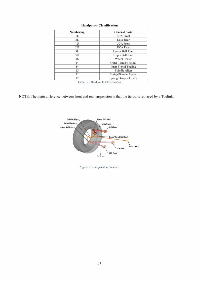
Hardpoints Classification

Numbering General Parts 1L LCA Front 2L LCA Rear 1U UCA Front 2U UCA Rear 5L Lower Ball Joint 5U Upper Ball Joint 16 Wheel Center 14 Outer Tierod/Toelink 44 Inner Tierod/Toelink 15 Spindle Align 11 Spring/Damper Upper 12 Spring/Damper Lower

Table 12 - Hardpoints Classification

NOTE: The main difference between front and rear suspension is that the tierod is replaced by a Toelink.

Figure 25 - Suspension Elements

52

4.2.1 Results

The kinematic performances were evaluated by means of the following quasi-static analyses: Static Ride Analysis, Static Roll Analysis and Steering analysis.

4.2.1.1 Static ride analysis The Static Ride Analysis allows to simulate the symmetrical shaking motion of the wheels of the same axle, evaluating the entire excursion guaranteed by the kinematic mechanism provided by the suspension system.

Simulation Parameters

Vehicle end Type of suspension

Tire static loaded radius [mm]

Tire vertical spring rate

[N/mm]

Jounce travel

[mm]

Rebound travel

[mm] Front Independent 343 200 60 50 Rear Independent 343 200 60 50

Table 13 - Static Ride Analysis Input

Figure 26 - Camber Angle vs Wheel Center Vertical Displacement

53

Figure 27 - Toe Angle vs Wheel Center Vertical Displacement

Figure 28 - Track Width vs Wheel Center Vertical Displacement

54

Figure 29 - SVSA Vertical Location vs Wheel Center Vertical Displacement

Figure 30 - Anti-Dive Percentage vs Wheel Center Vertical Displacement

55

Figure 31 - Anti-Squat Percentage vs Wheel Center Vertical Displacement

Figure 32 - Motion Ratio vs Wheel Center Vertical Displacement

56

Figure 33 - Scrub Radius vs Wheel Center Vertical Displacement

Figure 34 - Caster Trail vs Wheel Center Vertical Displacement

57

It is worth noting that Toe angle is always less than 1° and positive, which allows to improve the understeering gradient. The maximum track width is 20 mm. A negative scrub radius was obtained over the entire stroke in order to reach a stabilizing effect as previously discussed, while the Caster Trail has a variation of 5 mm in both compression and extension stroke.

4.2.1.2 Static roll analysis The Static Roll Analysis allows to simulate the asymmetrical shaking motion of the wheels of the same axle and it provides a series of useful indications for the evaluation of the kinematics and the roll dynamics.


Vehicle end Type of Suspension Tire Static loaded Radius

[mm]

Tire Vertical Spring Rate

[N/mm]

Roll Angle

[deg] Front Independent 343 200 2.5 Rear Independent 343 200 2.5

Table 14 - Static Roll Analysis Input

The results in terms of Camber and Roll Center Height are shown below:

Figure 35 - Camber Angle vs Roll Angle

58

Figure 36 - Roll Center Height vs Roll Angle

It is possible to see that the roll axis location is stable, moreover it is swooping. The latter datum results in a higher understeer gradient.

The recovery of camber during roll motions is partial. A camber of 1.5 deg of the external wheel is obtained at a 2 deg roll, which is not that negative. This is the result of a good compromise with the minimization of track variations, because the latter is in contrast with the camber recovery.

4.2.1.3 Steering analysis A Steering Analysis was conducted to verify that the specifications mentioned before are satisfied. This analysis consists in applying steering angles between a minimum and a maximum value in order to evaluate the performance output of the Camber, Caster Trail and the Ackermann deviation.


Vehicle end

Type of Suspension

Tire Static Loaded Radius [mm]

Tire Vertical Spring Rate [N/mm]

Maximum Steering Angle [deg]

Front Independent 343 200 320 Table 15 - Steering Analysis Input

59

Figure 37 - Camber Angle vs Steering Wheel Angle

Figure 38 - Caster Trail vs Steering Angle

60

Figure 39 - Ackermann Error vs Steering Wheel Angle

The internal Camber angle is positive and the external is negative, and as a consequence the Camber recovery increases when the car rolls during a cornering and the caster trail remains always positive.

The following table shows the output parameter related to the steering system, obtained by Multibody solver.

Output Parameters

Crub to Crub Diameter [m] Ackermann percentage [%] 11 90

Table 16 - Steering Analysis Results

61

4.3 Elastic elements

The aim of this section is to design the elastic elements, such as springs and roll bars, whose reference design criteria will be discussed later. The focus is on the vertical, roll and pitch dynamics.

The input data required are reported below:

Input Data

NOTE: The model includes the driver and passenger masses both of 75 Kg.

4.3.1 Ride motion

As mentioned before, the model used is the Quarter Car Model (3) at two degree of freedom. It is a simplified model at lumped parameters with the assumptions of rigid body and linear system.

Figure 40 - Quarter Car Model 2 DOF. (QCM, obtained from https://www.researchgate.net/figure/A-quarter-Car-Model_fig1_281595248 )

The stiffnesses of the springs were obtained considering the following criteria:

• Ride natural frequencies between 1-1.3 Hz; • Maximum static deformation of 15 mm at full load; • Rear ride frequencies higher than 15% compared to the front.

The latter improves the ride comfort when the car crosses the speed bumps because the stiffer rear axle minimizes the pitching motions.

Sprung Mass

[Kg]

Unsprung Mass

[Kg]

Tire Stiffness

[N/mm]

Center Mass Height

[mm]

Wheelbase

[mm]

a

[mm]

b

[mm] 157 18 200 350 2350 1175 1175

Table 17 - Elastic Elements Input Data

https://www.researchgate.net/figure/A-quarter-Car-Model_fig1_281595248

https://www.researchgate.net/figure/A-quarter-Car-Model_fig1_281595248

62

It can be shown that the second criterion is more restrictive than the first, hence the latter is not considered. Consequently, the frequencies in ride will be higher than the maximum imposed but this is not a relevant problem since the project concerns a mini sport car.

The static deformation is calculated at full loaded vehicle (with one additional passenger) as follows:

𝑓𝑠𝑡𝑎𝑡𝑖𝑐 =

∆𝑚𝑔

𝐾𝑤ℎ𝑒𝑒𝑙

(7)

∆𝑚 is the mass variation due to the load and 𝐾𝑤ℎ𝑒𝑒𝑙 is the wheel rate, which is the stiffness of an equivalent spring applied to the wheel center. This formula results from the starting assumption that the springs are preloaded to have zero static deformation of the vehicle with the driver alone.

By the stiffnesses 𝐾𝑤ℎ𝑒𝑒𝑙 it is possible to calculate the Ride Rate, which is the combination of tire stiffness and wheel rate.

𝐾𝑟𝑖𝑑𝑒 =

𝐾𝑤ℎ𝑒𝑒𝑙𝐾𝑡𝑖𝑟𝑒

𝐾𝑡𝑖𝑟𝑒 + 𝐾𝑟𝑖𝑑𝑒

(8)

Where 𝐾𝑡𝑖𝑟𝑒 is the vertical stiffness of the tire that is estimated by the following empirical relation [24]:

𝐾𝑡𝑖𝑟𝑒 = 0.00028𝑃√(−0.004𝐴𝑅 + 1.03) × 𝑆𝑁 × (

𝑆𝑁 × 𝐴𝑅

50+ 𝐷𝑅) + 3.45

(9)

where:

P = Pressure - kPa

AR = Aspect Ratio

SN = Nominal Section Width - mm

DR = Rim Diameter Code – mm

Ktire= Tire Vertical Stiffness – Kg/mm

An inflation pressure of 250 kPa was assumed, while other parameters are known by the tire size, which in this case study is 155/60R20. The result is a stiffness of 200 N/mm.

Finally, the spring stiffness is expressed by the following formula:

𝐾𝑠𝑝𝑟𝑖𝑛𝑔 =𝐾𝑤ℎ𝑒𝑒𝑙 −

𝜕𝑀𝑅𝜕𝑧𝑤

𝑃𝐿

𝑀𝑅2− 𝐾𝑏𝑢𝑠ℎ

(10)

Where 𝑃𝐿 is the spring preload, 𝐾𝑏𝑢𝑠ℎ is the stiffness contribution due to bushing and 𝑀𝑅 is the motion ratio, defined as the ratio between the deformation of the spring and the wheel ride.

63

Output Results

Parameters

Unit of Measure Front Axle Rear Axle

𝐾𝑟𝑖𝑑𝑒

[N/mm] 12.61 16.99

𝐾𝑡𝑖𝑟𝑒

[N/mm] 200 200

𝐾𝑤ℎ𝑒𝑒𝑙

[N/mm] 13.46 18.57

𝑀𝑅

[-] 0.540 0.639

𝑃𝐿

[N] 2511 2122

𝜕𝑀𝑅

𝜕𝑧𝑤

[1/mm] 1.3×10-4 6.5×10-4

𝐾𝑠𝑝𝑟𝑖𝑛𝑔

[N/mm] 32.83 22.65

𝐾𝑏𝑢𝑠ℎ𝑖𝑛𝑔

[N/mm] 12.16 19.31

𝑓𝑟𝑖𝑑𝑒

[Hz] 1.38 1.59

𝑓𝑠𝑡𝑎𝑡𝑖𝑐

[mm] 13.7 9.9

Table 18 - Vertical Stiffness Results

4.3.2 Pitch motion A further goal of the project is to obtain a pitch gradient PG less than 3 deg/g, that is calculated considering the ideal braking condition at laden vehicle, that is the most critical load case with maximum acceleration of 𝜇𝑔. As a starting hypothesis, the favorable anti-dive effects due to suspension linkages are neglected in order to be more cautious.

By using the simplified braking model (4), the longitudinal load transfer is:

∆𝐹𝑧 = 𝑚𝜇𝑔

ℎ

𝐿

(11)

Hence, the pitch gradient is calculated as follows:

∆𝑧𝐹 =

∆𝐹𝑧

𝑘𝑅𝑖𝑑𝑒,𝐹, ∆𝑧𝑅 =

∆𝐹𝑧

𝑘𝑅𝑖𝑑𝑒,𝑅

(12)

𝑃𝐺 = atan (

∆𝑧𝐹 + ∆𝑧𝑅

𝜇)

(13)

The obtained result is a pitch gradient of 1.78 deg/g; therefore, it was not necessary to improve the anti-dive characteristic. For this reason, the longitudinal rotation center of the front suspension is located below the wheel center in order to improve comfort when the car crosses speed bumps; while for the rear suspension the vice versa is valid, i.e. the rotation center must be above the wheel center while it is still maintaining high anti-squat and anti-dive percentages.

64

4.3.3 Roll motion

As a project target, a maximum roll gradient of 3 deg/g has been imposed, since at higher value the camber recovery is not enough to keep the outer wheel almost orthogonal.

The maximum lateral acceleration calculated is 0.9 g, which is due to the maximum grip.

At this point, it is necessary to calculate the roll stiffness 𝐾𝑟𝑜𝑙𝑙 request to satisfy the target mentioned above. For this purpose, the simplified lateral dynamic model (5) was used:

𝐾𝑟𝑜𝑙𝑙 = 𝐾𝑟𝑖𝑑𝑒

𝑡2

2+ 𝐾𝑏

(14)

𝐾𝑟𝑜𝑙𝑙 =

𝑚𝑎𝑦(ℎ − 𝑞) cos 𝜑 + 𝑚𝑔(ℎ − 𝑞) sin 𝜑

𝜑

(15)

where q is the roll center, 𝐾𝑏 is the stiffness of the anti-roll bar and the numerator represents the roll moment due to the centrifugal and weight force while the denominator is the roll angle.

Output Results

Parameters

Unit of Measure Front Axle Rear Axle

𝐾𝑟𝑖𝑑𝑒

𝑡2

2

[Nm/deg] 198 273

𝐾𝑏

[Nm/deg] 75 0

𝐾𝑟𝑜𝑙𝑙

[Nm/deg] 273 273

Table 19 - Roll Stiffness Results

The stabilizer bar is set to balance the stiffnesses of the front and rear axle.

65

4.4 Shock absorber

The main cause of the vehicle vibrations is due to road irregularities, which cannot be reproduced by deterministic signals, given the high randomness of the process. For this purpose, road excitations were evaluated using an approach that refers to the theory of statistical signals. Reference is made to the function of Power Spectral Density with the hypothesis of the stationary and ergodic process.

The determination of the damping coefficient and of the workingspace of the suspension will be discussed in this paragraph with the aim of optimizing comfort and at the same time to ensure good vehicle handling.

The model used for these analyses remains the same as before, whose inputs are reported below.

Input Data

Vehicle End

𝒄𝒓

[m2/cycle]

n

[-]

Vehicle Speed

[km/h]

Frequencies range 𝒇𝒓𝒂𝒏𝒈𝒆 [Hz]

Damping range

[Nmm/s]

Wheel Rate

[N/mm]

Sprung Mass

[Kg]

Unsprung Mass

[Kg]

Front 1.024×10-5 2 90 0÷25 copt×(0.8÷1.2) 13.46 157 18 Rear 1.024×10-5 2 90 0÷25 copt×(0.8÷1.2) 18.57 157 18

Table 20 - Damper Elements Input

4.4.1 Damping coefficient

The FRF (6) of the acceleration and vertical force and their Root Mean Square value were computed for different damping coefficient of the shock absorber. The last function allows to evaluate the effect of damping on acceleration and force in order to choose an appropriate value.

The formulation of PSD used to perform the analysis (measured in 𝑚2/𝐻𝑧) is the following:

𝑆 = 𝑐𝑟𝑉𝑛−1𝜔−𝑛

(16)

Where 𝑐𝑟 (𝑚3𝑐𝑦𝑐𝑙𝑒 𝑚⁄ ) is the empirical coefficient dependent on the road profile, n is a nondimensional constant equal to 2, 𝑉 (𝑚 𝑠⁄ ) is the vehicle speed and finally 𝜔 (𝐻𝑧) is the frequency of excitation. The first parameter is available by the standard ISO 8606:1995 that subdivides road profiles into eight classes, indicated by letters from A to H. In this case the class D was considered, which represents the worst condition of a hard-surfaced road [21].

The rms functions of vertical acceleration and dynamic forces are:

𝑎𝑟𝑚𝑠 = √∫ 𝜔4𝐻2𝑆𝑑𝜔

𝜔2

𝜔1

(17)

𝐹𝑟𝑚𝑠 = √∫ 𝜔4𝐻𝐹

2𝑆𝑑𝜔𝜔2

𝜔1

(18)

where 𝐻 and 𝐻𝐹 are respectively the frequency gain related to the vertical displacement and vertical forces obtained by the FRF analysis.

66

The optimal wheel damping 𝐶𝑤ℎ𝑒𝑒𝑙,𝑜𝑝𝑡 that minimizes the maximum acceleration is the following:

𝐶𝑤ℎ𝑒𝑒𝑙,𝑜𝑝𝑡 = √

𝐾𝑤ℎ𝑒𝑒𝑙𝑚𝑠𝑝𝑟𝑢𝑛𝑔

2× √

2𝐾𝑤ℎ𝑒𝑒𝑙 + 𝐾𝑡𝑖𝑟𝑒

𝐾𝑡𝑖𝑟𝑒

(19)

The correlation between wheel damping and damping coefficient of the shock absorber is:

𝐶𝑠ℎ𝑘 𝑎𝑏𝑠 =

𝐶𝑤ℎ𝑒𝑒𝑙

𝑀𝑅2

(20)

4.4.2 Workingspace

Workingspace of the suspension was obtained as the maximum value between these conditions:

• The base formula used to compute the working space is the following:

𝑤𝑠 =

∆𝑚

𝑚𝑣

𝑔

(2𝜋𝑓𝑟𝑖𝑑𝑒)2+ 3𝑟𝑚𝑠𝑠,𝑙 + 3𝑟𝑚𝑠𝑠,𝑢

(21)

the first term represents the mass variation due to load with respect to unladen mass, while the second and

third are respectively the root mean square of the displacements at laden and unladen vehicle

• The suspension travel, excluding the end of the stroke, must be equal at least to the maximum

deformation in worst load condition that is referred to vehicle in the ideal braking condition. The minimum suspension travel is calculated as: 𝑆𝑇𝑐𝑜𝑚𝑝,𝑚𝑖𝑛 = ∆𝑧𝑐,𝑙 + 𝛿, 𝑆𝑇𝑒𝑥𝑡,𝑚𝑖𝑛 = ∆𝑧𝑒,𝑢 + 𝛿,

(22)

𝑆𝑇𝑚𝑖𝑛 = 𝑆𝑇𝑐𝑜𝑚𝑝,𝑚𝑖𝑛 + 𝑆𝑇𝑒𝑥𝑡,𝑚𝑖𝑛 (23)

where 𝛿 = 15 𝑚𝑚 is the end of the stroke assumed, while ∆𝑧𝑐,𝑙 and ∆𝑧𝑒,𝑢 are respectively the compression and extension of the suspension at laden and unladen vehicle. These values are valid for both axles since the same suspension travel is required.

67

4.4.3 Results

The aim of this paragraph is to present and discuss the results concerning the diagrams of rms functions, and the choice of damping coefficient and suspension’s workingspace.

Figure 41 - Vertical Acceleration RMS vs Vertical Force RMS, Front Suspension

Figure 42 - Vertical Acceleration RMS vs Vertical Force RMS, Rear Suspension

68

The wheel damping coefficients used are 820 and 1076 (Ns/m) for the front and the rear suspension, respectively. They correspond to the minimum rms acceleration in the diagrams above. This is intended to improve comfort, which has been previously neglected by adopting springs with higher stiffness compared to the stiffness considered for standard target. The latter has already been discussed above.

Moreover, it has been verified that the three times of root mean square of the force is less than the static load, which will avoid the risk of lifting of the vehicle.

Output Results

Vehicle End

Minimum Workingspace 𝒘𝒔

[mm]

Minimum Suspension Travel

𝑺𝑻𝒎𝒊𝒏

[mm]

Effective Suspension Travel 𝑺𝑻𝐞𝐟𝐟

[mm]

𝑪𝒘𝒉𝒆𝒆𝒍

[Ns/mm]

𝑪𝒔𝒉𝒌 𝒂𝒃𝒔

[Ns/mm] Front 67.32 98 110 0.82 2.81 Rear 67.26 98 110 1.08 2.64

Table 21 - Damping Analysis Results

The minimum suspension travel in compression is 60 mm and in extension is 38 mm. The final travel is subdivided as 60 mm in jounce and 50 in rebound.

69

4.5 Bushing

Since the choice of the bushing can affect the drivability aspects, which is one of the concerns of this project, it is necessary to minimize the variation of the suspensions' static parameters following the application of the operating loads. To reach this aim, the force tests and their corresponding targets are the following:

1) Lateral Force test:

• Maximum Toe Angle for 1 kN of lateral force equal to 0.2 deg/kN; • Maximum Camber Angle for 1 kN of lateral force equal to 0.2 deg/kN; • Maximum Lateral Displacement of wheel center for 1 kN of lateral force equal to 2 mm/kN.

2) Braking Force test:

• Maximum Toe Angle for 1 kN of longitudinal force equal to 0.14 deg/kN; • Maximum Caster Angle variation for 1 kN of longitudinal force equal to 1 deg/kN.

3) Driving Force test:

• Maximum wheel center displacement of 10 mm.

The supplier for the bushings is FIBET and the product specifications of the chosen bushing connections are the following:

Figure 43 - FIBET Bushing. [25]

Product Code

d

[mm]

D

[mm]

I

[mm]

L

[mm]

Radial Stiffness [N/mm]

Axial Stiffness [N/mm]

Torsional Stiffness [Nm/deg]

Conical Stiffness [Nm/deg]

Weight

[g] FBNA

1025.3541

10

25

25

41

14830

104

1.75

13.76

75 Table 22 - Bushing Characteristics

70

The FBNA range of bushes are designed to eliminate high frequencies whilst support high loads during operation. This is achieved through elastic deformation of the rubber under the effect of the external force being applied to the metal tubes [25]. This allows to improve comfort.

This choice is to be considered preliminary as it should be proven by means of a detailed NHV analysis which in turn removes the hypothesis of rigid suspension linkages.

The parameters required by the simulations are displayed in the table below, and they are to be considered indicative since the main interest is obtaining the above-mentioned gradients.

Input Parameters

Vehicle End Maximum Lateral Force

[N]

Maximum Braking Force

[N]

Maximum Driving Force

[N] Front 2500 2500 0 Rear 2500 2500 2500

Table 23 - Compliance Test Input

4.5.1 Results

The results related to the force tests, mentioned above, are reported as follows.

4.5.1.1 Lateral force test

Figure 44 - Toe Angle vs Lateral Force

71

Figure 45 - Camber Angle vs Lateral Force

Figure 46 - Wheel Center Lateral Displacement vs Lateral Force

72

4.5.1.2 Braking force test

Figure 47 - Toe Angle vs Braking Force

Figure 48 - Caster Angle vs Braking Force

73

4.5.1.3 Driving test

Figure 49 - Wheel Center Longitudinal Displacement vs Driving Force

74

4.6 Bump stops

The internal bumpers of the suspension are used not only to limit the travel of the suspension, but also to absorb the impacts that come from strong road irregularities. They are normally housed along the shock rod or even on the suspension arm or on the frame and they provide additional resistance during the last compression and extension phases of the suspension.

It was chosen to install them coaxially with respect to the shock absorber stem so that they act 15 mm before the end of the stroke.

The bumpers were set so that they can absorb in maximum compression a load equal to three or four times the static one, and in maximum extension they will give a null force.

Figure 50 - Vertical Force vs Wheel Center Vertical Displacement

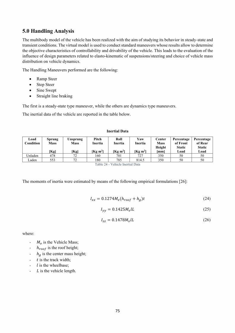
75

5.0 Handling Analysis The multibody model of the vehicle has been realized with the aim of studying its behavior in steady-state and transient conditions. The virtual model is used to conduct standard maneuvers whose results allow to determine the objective characteristics of controllability and drivability of the vehicle. This leads to the evaluation of the influence of design parameters related to elasto-kinematic of suspensions/steering and choice of vehicle mass distribution on vehicle dynamics.

The Handling Maneuvers performed are the following:

• Ramp Steer • Step Steer • Sine Swept • Straight line braking

The first is a steady-state type maneuver, while the others are dynamics type maneuvers.

The inertial data of the vehicle are reported in the table below.

Inertial Data

Load Condition

Sprung Mass

[Kg]

Unsprung Mass

[Kg]

Pitch Inertia

[Kg m2]

Roll Inertia

[Kg m2]

Yaw Inertia

[Kg m2]

Center Mass

Height [mm]

Percentage of Front

Static Load

Percentage of Rear Static Load

Unladen 478 72 160 701 727 350 50 50 Laden 553 72 180 785 814.5 350 50 50

Table 24 - Vehicle Inertial Data

The moments of inertia were estimated by means of the following empirical formulations [26]:

𝐼𝑥𝑥 = 0.1274𝑀𝑣(ℎ𝑟𝑜𝑜𝑓 + ℎ𝑔)𝑡

(24)

𝐼𝑦𝑦 = 0.1425𝑀𝑣𝑙𝐿

(25)

𝐼𝑧𝑧 = 0.1478𝑀𝑣𝑙𝐿 (26)

where:

- 𝑀𝑣 is the Vehicle Mass; - ℎ𝑟𝑜𝑜𝑓 is the roof height; - ℎ𝑔 is the center mass height; - 𝑡 is the track width; - 𝑙 is the wheelbase; - 𝐿 is the vehicle length.

76

Figure 51 shows the vehicle model.

Figure 51 - Vehicle Model

77

5.1 Ramp Steer

A Ramp Steer event simulates a ramped steer input into a vehicle driving at a steady speed and it is typically used to predict the steady state dynamic response of the vehicle. A drive torque controller is added to maintain constant speed during the event to drive the vehicle forward [27].

Input Data

Initial Steer [deg]

Steer Ramp Rate [deg/s]

Maximum Steer [deg]

Velocity [Km/h]

0 10 100 80 Table 25 - Ramp Steer Input Data

5.1.1 Results

Figure 52 - Steer Angle vs Lateral Acceleration

78

Figure 53 - Side Slip Angle vs Lateral Acceleration

Figure 54 - Average Slip Angle vs Lateral Acceleration

79

Figure 55 - Roll Angle vs Lateral Acceleration

Figure 56 - Yaw Rate vs Lateral Acceleration

80

Figure 57 - Vertical Force vs Lateral Acceleration, Unladen Vehicle

Figure 58 - Vertical Force vs Lateral Acceleration, Laden Vehicle

81

Output Results

Gradients respect to Lateral Acceleration Unit of Measure

Values at Unladen Vehicle

Values at Laden Vehicle

Understeer [deg/m/s2] 0.2 0.2 Side Slip Angle [deg/m/s2] 0.20 0.19

Yaw Rate [deg/s/m/s2] 2.66 2.66 Roll [deg/m/s2] 0.26 0.29

Gain respect to Steer Angle Lateral Acceleration [m/s2/deg] 0.14 0.14

Yaw Rate [s-1] 0.32 0.32 Side Slip Angle [-] 0.02 0.02

Table 26 - Ramp Steer Results

The understeer gradient is approximately equal to 2 deg/g, a common value for normal cars. It is known that the low weight of the vehicle reduces the understeer gradient; hence it is needed to mount different tires on the front and rear axle to obtain an acceptable value.

The Front Total Lateral Load Transfer Distribution (FTLLTD) is 0.49, almost equal to the expected value of 0.5. The load transfer is not symmetric because the springs are not perfectly linear. The springs are stiffer in compression than in extension because of the variation of the motion ratio, even if it is slight. This is less in the front than in the rear axle. Hence, in the latter there is a greater asymmetry, however slight. In particular, the load of the rear left wheel is higher than the load on the front left wheel, which is the expected load value. However, this is not a serious problem: the variation of the motion ratio can be reduced by intervening on the position of the springs.

It is worth noticing that the maximum lateral acceleration is equal to the grip limit, which is 0.88 g. This means that the Camber Recovery is enough to maintain the outer wheel orthogonal. In the previous Roll Analysis of the suspensions this result was not visible because it is only an asymmetrical shaking motion of the wheels that does not include the roll motion of the body.

The maximum Roll Angle is 2.25 and 2.55 deg respectively at the unladen and laden condition. They are approximately equal to the expected values.

82

5.2 Step Steer

A Step Steer event simulates the vehicle response to a sudden step input to the steering wheel. A drive torque controller is added to maintain speed constant during the event to drive the vehicle forward [28]. The characteristic values and functions in time domain necessary to characterize the vehicle transient response are [29]:

- Time response of lateral acceleration, yaw rate and roll angle; - Time lags between steering-wheel angle, roll angle and yaw rate; - Overshoot value of roll angle, yaw rate and lateral acceleration.

Input Data

Time of step [s]

Function Type Maximum Steer [deg]

Steer Ramp Rate [deg/s]

Velocity [Km/h]

1 Ramp 27 200 80 Table 27 - Step Steer Input Data

5.2.1 Results A maximum Steer Angle of 27 deg was imposed to reach the lateral acceleration of 0.4 g.

Figure 59 - Steer Angle vs Time

83

Figure 60 - Lateral Acceleration vs Time

Figure 61 - Side Slip Angle vs Time

84

Figure 62 - Roll Angle vs Time

Figure 63 - Yaw Rate vs Time

85

Output Results

Time Response Unit Values at Unladen Vehicle

Values at Laden Vehicle

Roll Angle [s] 0.34 0.32 Yaw Rate [s] 0.16 0.15 Overshoot

Lateral Acceleration [%] 2.4 2.5 Yaw Rate [%] 8.2 8.6

Time of Maximum Amplitude Yaw Rate [s] 1.4 1.39

Lateral Acceleration [s] 1.68 1.62 TB Factor [deg s] 0.3 0.26

Table 28 - Step Steer Results

The time response is the difference between the time at 90% of the steady state response and the time at 50% of the ramp. This parameter is used to evaluate the delay between input and output. The maximum recommended values are 0.45 s and 0.35 s respectively for the Roll Angle and Yaw Rate.

Overshoot is the percentage increment between the peak value of the response and the steady-state value. In this case they are very low.

Finally, the TB Factor is the product of the steady-state side slip angle and the time of maximum amplitude of the yaw-rate. This parameter should be as low as possible and 0.5 (deg s) is the maximum acceptable value for the vehicle to respond quickly.

86

5.3 Swept Sine

A Swept Sine event simulates a vehicle driving at a constant speed with a sinusoidal steering input of constant magnitude but increasing frequency applied. A Drive torque controller is used maintain the constant velocity of the vehicle [30].

This test is used to obtain the frequency response of lateral acceleration, yaw rate, side slip angle and roll angle to evaluate the capability of the vehicle to respond at high frequency.

Input Data

Start Time

[s]

End Time

[s]

Maximum Steer

[deg]

Frequency Rate

[Hz/s]

Frequency Range [Hz]

Velocity

[Km/h] 2 12 21 0.275 0.2÷3 80

Table 29 - Swept Sine Input Data

5.3.1 Results Steering wheel angle (SWA) amplitude is fixed at value of 21 deg to reach a lateral acceleration of 0.3 g. SWA is imposed with sinusoidal law at increasing frequency.

Figure 64 - Steer Angle vs Time

87

Figure 65 - FRF Yaw Rate Gain

Figure 66 - FRF Lateral Acceleration Gain

88

Figure 67 - FRF Roll Gradient

Output Results

Metric Unit Value at Unladen Vehicle

Value at Laden Vehicle

Steady-state Lateral Acceleration Gain [g/deg] 0.015 0.014 Minimum Lateral Acceleration Gain [g/deg] 0.003 0.003

Frequency at Maximum Lateral Acceleration Gain [Hz] 0.30 0.29 Maximum Yaw Rate Gain [1/s] 0.42 0.40

Steady-state Yaw Rate Gain [1/s] 0.40 0.38 Frequency at Maximum Yaw Rate Gain [Hz] 0.85 1.00

Yaw Rate Amplification Ratio [-] 1.05 1.05 Steady-state Roll Gradient [deg/g] 2.55 2.84 Maximum Roll Gradient [deg/g] 10 11

Frequency at Maximum Roll Gradient [Hz] 2.2 2.2 Roll Gradient Amplification Ratio [-] 3.92 3.87 Lateral Acceleration Delay @1 Hz [ms] 14 13

Yaw Rate Delay @0.2 Hz [ms] 69 65 Yaw Rate Delay @1 Hz [ms] 87 83 Roll Angle Delay @1 Hz [ms] -50 -50

Table 30 - Swept Sine Results

89

One of the common methods to study the vehicle dynamics characteristics is to observe its response to periodic steering. In particular, the driver is sensitive to the yaw rate changes in relation to the steering angle.

For this purpose, the ratio between the peak gain value and the gain value at low frequency (f =0.2 Hz) is used to represent the vehicle controllability. In this case, Yaw Rate gain is almost constant until 1.5 Hz, while at higher frequencies it decreases in according with the reduction of the grip. The Yaw Rate Gain peak value is almost equal to the static one, which means greater controllability of the vehicle. The peak and the static value are respectively equal to 0.42 and 0.40 (1/s). They are slightly greater than the typical value of the normal passenger car because mini cars have a smaller wheelbase. This is a limit for this vehicle, which increases the Yaw Rate Gain. However, given the low velocity involved for this vehicle, this is not a problem.

The delay of the Yaw Rate, with respect to the instant of application of the steering input, is less than 100 ms as the frequency changes. This guarantees the possibility of making sudden changes of direction.

Lateral acceleration gain is almost constant until 0.5 Hz, while at a higher frequency it decreases first and then stabilizes. This result is acceptable. The ideal situation is to have constant gain at least at 1 Hz, but it is not possible, given the limited weight of the car that reduces the maximum friction forces transmittable.

Roll gradient is almost constant until 1.2 Hz and then there is a resonance peak with a maximum value of 10 deg/g at 2.2 Hz. Fortunately, the resonance frequency is higher than the frequency rage in normal driving condition.

Figure 68 - Driver Sensitive. (Vehicle Handling Dynamics: Theory and application. Page 278)

90

5.4 Straight line braking

This test allows to simulate the braking maneuver during which the car, starting from an initial forward speed, slows down at constant deceleration until it stops on the straight. The steering wheel is normally held fixed and a braking torque controller applies torque at the wheels to slow the vehicle [31].

The multibody simulation software requires as inputs the initial vehicle speed, the desired deceleration level, and the Braking Torque Distribution (Braking Bias). The first is imposed at 90 km/h and the deceleration level at 1g, which are respectively the maximum speed and the grip limit with friction coefficient µ equal to 1. The Braking Bias was calculated by evaluating the ideal braking parabola which provides the combination of braking forces on the two axles for each acceleration condition, to guarantee the same friction coefficient (with the hypothesis of a flat road):

(𝐹𝑥,𝐹 + 𝐹𝑥,𝑅)

2− 𝑚𝑔 (𝐹𝑥,𝐹

𝑎

ℎ− 𝐹𝑥,𝑅

𝑏

ℎ) = 0

(27)

Therefore, the ideal distribution of braking torque between the two axles has been identified, in order to ensure overall application of a braking force equal to 65% of the total braking force at the front end, intersecting the ideal braking parabola with the constant straight line deceleration expressed by the relation:

𝐹𝑥,𝐹 + 𝐹𝑥,𝑅 = 𝑚𝑔

(28)

Finally, the following diagram was obtained considering an unloaded vehicle.

Figure 69 - Braking Force Distribution

91

This analysis is very qualitative, because the brakes are of regenerative type in electric cars with the integration of hydraulic brakes for emergency cases. Therefore, the braking torque distribution is not fixed but can vary according to the control logic of the system. This analysis is useful not only to evaluate the handling behavior, but also to estimate the braking torque in order to give these data to the supplier who will provide an adequate solution, as well as the physical product. Hence, given the qualitative information of this test, the simulation was conducted only at unladen vehicle.

Input Data

Load Condition Velocity [Km/h] Deceleration [g] Braking Bias Unladen 90 1 1.84

Table 31 - Braking Analysis Input Data

5.4.1 Results

Figure 70 - Wheel Torque vs Time

92

Figure 71 - Velocity vs Longitudinal Displacement

Figure 72 - Longitudinal Slip vs Time

≅ 37m

93

Figure 73 - Vertical Displacement vs Deceleration

Figure 74 - Pitch Angle vs Deceleration

94

The steady-state torque will be useful to design the braking system. The braking torque applied is 780 and 420 Nm on the front and rear wheels, respectively. The braking distance is approximately 37 m at the initial speed of 90 km/h.

The longitudinal steady-state slip angle is lower than the maximum value, which is 10%, after which instability will be experienced.

The pitch gradient is very low, as expected on the basis of the previous calculations. This is due to the considerable stiffness of the springs and the anti-dive contributions provided by the linkages. Furthermore, the suspensions never collide with the internal bumpers.

95

5.5 Double lane change

A Double Lane Change event drives the vehicle through a lane change and a return to lane maneuver, attempting to follow the centerline of the defined lane. You can define the speed of the lane change, along with the lane dimensions. A steer controller is used to follow the path and a drive torque controller is used to maintain speed throughout the event. The event supports right and left lane changes.

The event is designed to simulate a sudden turn in one direction, a short recovery period, and a return to the original lane of travel. The event simulates obstacle avoidance transient vehicle dynamics. The vehicle path is defined in the full vehicle dataset in the Double Lane Change analysis. A driver model attempts to make the CG of the body follow the defined path.

Figure 75 - Vehicle Path DLC. [32]

The Double Lane Change event path is shown in the diagram above. Lane dimensions are entered in meters and are translated to millimeters in the various locations they are used (point parametric definitions, solver arrays, and so on). The lane graphics are defined from the path dimensions and are used to illustrate the path. The road surface used by the tire is defined by the .rdf file in the tire system and is independent from the graphics.

The event is like the ISO event 3888-2 “Passenger Cars-Test track for a severe lane change maneuver-Part 2: Obstacle avoidance”. The ISO event defines a test track setup of lanes and cones. The lane width is a function of the vehicle width and any path is permitted if the cones are not disturbed [32].

Input Data

Velocity [km/h] 65 Lane Change Direction Left Length - Section 1 [m] 15 Length - Section 2 [m] 30 Length - Section 3 [m] 25 Length - Section 4 [m] 25 Length - Section 5 [m] 15

Lateral Offset [m] 3.5 Table 32 - DLC Input Data

96

5.5.1 Results

The maximum achievable vehicle speed in this test is 65 km/h.

Figure 76 - Vehicle CG Displacement, Unladen Vehicle

Figure 77 - Vehicle CG Displacement, Laden Vehicle

97

Figure 78 - Lateral Acceleration vs Distance

Figure 79 - Yaw Rate vs Distance

98

Figure 80 - SWA vs Distance

Figure 81 - Roll Angle vs Distance

99

As can be seen, there are significant oscillations of the Yaw Rate. This is due to the high values of the Yaw Rate Gain, as shown before. However, the Yaw-Damping helps to quickly reduce these oscillations. In the experimental tests, the vehicle speed is not constant because in the second lane change the throttle is released. This is favorable to the vehicle control because it allows to reduce the oscillations. Moreover, the steering angle fluctuations aim to keep the vehicle in the lane as much as possible. These are due to the steering controller which simulates the driver.

100

6.0 Braking System In a battery-powered electric vehicle regenerative braking is the conversion of the vehicle’s kinetic energy

into chemical energy stored in the battery, where it can be used later to drive the vehicle. It is braking because it also serves to slow the vehicle [33]. Furthermore, the ability to brake the vehicle is interrupted at low speeds, which is why the regenerative brake cannot be considered a substitute but an assistant to the traditional braking system. At low speeds, the rotor (present inside the electric motor) has an insufficient angular speed to generate the potential necessary to obtain a correct braking effect. The efficiency of the generator is significantly reduced with the reduction of the angular speed of the rotor. This results in a drastic drop in braking force. For the complete stop of the vehicle, therefore, a traditional braking system that exploits friction is also necessary [34]. Another limitation is that the regenerative braking is necessarily limited when the batteries are fully charged. Because the additional charge from regenerative braking would cause the voltage of a full battery to rise above a safe level, our motor controller will limit regenerative torque in this case and the hydraulic traditional system supplies the integration of braking torque needed [33]. For effective braking and optimal regeneration, it is important to estimate the maximum braking force that could be applied without leading to a wheel lock situation [35].

The following figure shows an example of regenerative braking.

Figure 82 - Regenerative Brakes. [33]

101

In a hydraulic braking system, when the brake pedal is pressed, a pushrod exerts force on the piston in the master cylinder, causing fluid from the brake fluid reservoir to flow into a pressure chamber through a compensating port. This results in an increase in the pressure of the entire hydraulic system, forcing fluid through the hydraulic lines toward one or more calipers where it acts upon one or more caliper pistons sealed by one or more seated O-rings (which prevent leakage of the fluid). A brake booster is used to help the driver by decreasing the braking effort.

The brake caliper pistons then apply force to the brake pads, pushing them against the spinning rotor, and the friction between the pads and the rotor causes a braking torque to be generated, slowing the vehicle [36].

The ABS system manages the braking to avoid the wheels locking and guarantee the vehicle stability.

Figure 83 shows an example of an electro-hydraulic braking system layout.

Figure 83 - Hydraulic Braking System. (Highly Automated Vehicle System, https://www.researchgate.net/figure/Layout-of-an-Electro-Hydraulic-Braking-System-Source-Prof-von-Glasner_fig88_321527129)

https://www.researchgate.net/figure/Layout-of-an-Electro-Hydraulic-Braking-System-Source-Prof-von-Glasner_fig88_321527129

https://www.researchgate.net/figure/Layout-of-an-Electro-Hydraulic-Braking-System-Source-Prof-von-Glasner_fig88_321527129

102

6.1 Preliminary solution

For this vehicle, a regenerative brakes system was chosen with the integration of a standard hydraulic one. It was decided to buy both the product and the solution by a supplier that will be defined later.

However, a rough estimate of the diameter of the master cylinder and the maximum oil pressure was made, considering only a friction braking. For this purpose, the braking torque acting on the disc is given by the relation (29):

𝑇𝑏 = 𝑛µ𝑏𝑝𝑜𝐴𝑏𝑟𝑒

(29)

where:

- 𝑛: number of pads

- µ𝑏: friction coefficient

- 𝑟𝑒: mean radius of the disc

- 𝐴𝑏: area of the braking piston

- 𝑝𝑜: oil pressure

The steady-state torque is previously obtained by the braking test, whose values are approximately 800 Nm on the front wheels and 400 Nm on the rear ones at a maximum deceleration of 1 g. In the case of maximum torque, assuming a friction coefficient of 0.3, 𝐴𝑏 of 9.62×10-4 m2 and 𝑟𝑒 of 119 mm, the oil pressure is 57 bar with two pads and two pistons on the front brakes. On the rear axle, only one braking piston is applied to obtain a braking torque of 400 Nm.

The force acting on the Master Cylinder (MC) is calculated by the equation (30):

𝐹𝑚𝑐 = 𝑝𝑜

𝜋𝐷𝑖𝑛𝑡,𝑐𝑦𝑙2

4

(30)

If the system does not have the brake booster and the pedal force is 450 N with a leverage ratio of 4, the force on MC is 1800 N. Hence, the internal diameter obtained is 20 mm.

It is worth calculating the volume of fluid transported in the pistons and compare it with the one moved by the

master cylinder. As first estimate, the volume computed on the braking pistons is:

∆𝑉𝑝 = 2 × 𝑐 × 𝐴𝑏 × 𝑛𝑝 (31)

where c is the travel of the caliper, 𝑛𝑝 is the number of the braking pistons and the factor 2 is due to the two

wheels on the axle. The whole volume obtained, with the assumption of c equal to 0.7 mm, is 4×10-6 m3. This

volume must be less than the fluid volume moved in the master cylinder, calculated as follows:

∆𝑉𝑚𝑐 =

𝐶𝑝

𝜏×

𝜋𝐷𝑖𝑛𝑡,𝑐𝑦𝑙2

4≥ ∆𝑉𝑝

(32)

where 𝐶𝑝 is the maximum travel of the pedal, which is imposed equal to 100 mm, and 𝜏 is the leverage ratio. The volume ∆𝑉𝑚𝑐 is 7.9×10-6 m3, higher than ∆𝑉𝑝.

103

Finally, the characteristic of the pressure as function of the deceleration is computed by the correlation between braking torque and deceleration, assuming a linear law of the torque.

Figure 84 - Pressure vs Deceleration

These calculations are highly indicative but are useful to the supplier as a first basis for choosing the appropriate braking system.

104

7.0 Conclusions and future perspectives

In this thesis, the vehicle dynamics development of an electric quadricycle was presented. The study is focused on the vehicle dynamics aspects such as powertrain, braking system, steering and suspension design.

For future development, first, it will be necessary to use correct tire models and improve the design solutions.

Second, a detailed NVH analysis should be carried on to analyze the comfort and durability of the components because comfort has been analyzed using only simplified models. This new analysis should include the contributions of the bushings, non-linear damping, and the deformability of the suspension’s linkages. All this should be considered together with the mechanical design and setting of the battery layout, as well as the cells configuration.

Other fundamental check is the technic and economic feasibility of the solutions. The project has to be conducted respecting an established budget.

Finally, after a first realization, an experimental test phase will begin for the empirical characterization of the vehicle. Then, an experimental-numerical correlation will be necessary for the validation of the virtual model. The validation of the model will be assessed on the basis of both drivability and comfort.

Another future goal is the design of the same vehicle but in the race car version. This is because the vehicle was originally conceived as both a passenger and sport car.

105

References

[1] Zhanglin Cai, Stephen Chan, Xiaofeng Tang and Jiang Xin, The Process of Vehicle Dynamics Development, Papers.

[2] Thomas D. Gillespie, Fundamentals of Vehicle Dynamics, SAE International, 1992.

[3] Giancarlo Genta, Lorenzo Morello, L’AUTOTELAIO VOL. 1, PROGETTO DEI COMPONENTI, Levrotto & Bella, 2007.

[4] Vincenzo Domenico Vurro, Impostazione elastocinematica delle sospensioni di una vettura monoposto da competizione e analisi della dinamica veicolo, Tesi.

[5] Altair Connect, MotionView Overview, Altair MotionView Help Home. https://altairhyperworks.com/hwhelp/Altair/2019/help/mv/topics/motionview/motionview_overview_r.htm

[6] Altair Connect, Using MotionView, Altair MotionView Help Home. https://altairhyperworks.com/hwhelp/Altair/2019/help/mv/topics/motionview/motionview_using_r.htm

[7] Altair Connect, End User Workflow, Altair MotionView Help Home. https://altairhyperworks.com/hwhelp/Altair/2019/help/mv/topics/motionview/end_user_workflow_r.htm

[8] Altair Connect, Construct Models, Altair MotionView Help Home. https://altairhyperworks.com/hwhelp/Altair/2019/help/mv/topics/motionview/constructing_models_r.htm

[9] Altair Connect, Execute Solvers, Altair MotionView Help Home.

https://altairhyperworks.com/hwhelp/Altair/2019/help/mv/topics/motionview/solvers_execute_r.htm

[10] Altair Connect, Container Entities, Altair MotionView Help Home.

https://altairhyperworks.com/hwhelp/Altair/2019/help/mv/topics/motionview/container_entities_r.htm

[11] Altair Connect, Post-Processing, Altair MotionView Help Home.

https://altairhyperworks.com/hwhelp/Altair/2019/help/mv/topics/motionview/post_processing_r.htm#post_processing_r

[12] Altair Connect, MotionSolve User Guide, Altair MotionSolve Help Home. https://altairhyperworks.com/hwhelp/Altair/2019/help/ms/topics/getting_started/motionsolve_main_overview.htm

[13] Altair Connect, Modeling in MotionSolve, Altair MotionSolve Help Home.

https://altairhyperworks.com/hwhelp/Altair/2019/help/ms/topics/solvers/ms/modeling_in_motionsolve.htm

[14] Altair Connect, Analysis in MotionSolve, Altair MotionSolve Help Home. https://altairhyperworks.com/hwhelp/Altair/2019/help/ms/topics/solvers/ms/analysis_in_motionsolve.htm

[15] Altair Connect, Typical Outputs, Altair MotionSolve Help Home. https://altairhyperworks.com/hwhelp/Altair/2019/help/ms/topics/solvers/ms/typical_outputs.htm

[16] Altair Connect, Welcome to the Professional Edition of Altair Activate 2019.4, Altair Activate Help Home. https://solidthinking.com/help/2019.4/activate/professional/en_us/topics/getting_started/intro_activate_c.htm

[17] Altair Connect, Model Components, Altair Activate Help Home. https://solidthinking.com/help/2019.4/activate/professional/en_us/topics/math_solutions/model_creation_c.htm

https://altairhyperworks.com/hwhelp/Altair/2019/help/mv/topics/motionview/motionview_overview_r.htm

https://altairhyperworks.com/hwhelp/Altair/2019/help/mv/topics/motionview/motionview_using_r.htm

https://altairhyperworks.com/hwhelp/Altair/2019/help/mv/topics/motionview/end_user_workflow_r.htm

https://altairhyperworks.com/hwhelp/Altair/2019/help/mv/topics/motionview/constructing_models_r.htm

https://altairhyperworks.com/hwhelp/Altair/2019/help/mv/topics/motionview/solvers_execute_r.htm

https://altairhyperworks.com/hwhelp/Altair/2019/help/mv/topics/motionview/container_entities_r.htm



https://altairhyperworks.com/hwhelp/Altair/2019/help/ms/topics/getting_started/motionsolve_main_overview.htm

https://altairhyperworks.com/hwhelp/Altair/2019/help/ms/topics/getting_started/motionsolve_main_overview.htm

https://altairhyperworks.com/hwhelp/Altair/2019/help/ms/topics/solvers/ms/modeling_in_motionsolve.htm

https://altairhyperworks.com/hwhelp/Altair/2019/help/ms/topics/solvers/ms/analysis_in_motionsolve.htm

https://altairhyperworks.com/hwhelp/Altair/2019/help/ms/topics/solvers/ms/typical_outputs.htm

https://solidthinking.com/help/2019.4/activate/professional/en_us/topics/getting_started/intro_activate_c.htm

https://solidthinking.com/help/2019.4/activate/professional/en_us/topics/math_solutions/model_creation_c.htm

https://solidthinking.com/help/2019.4/activate/professional/en_us/topics/math_solutions/model_creation_c.htm

106

[18] Wikipedia, Powertrain.

https://en.wikipedia.org/wiki/Powertrain

[19] MAGELEC PROPULSION, Official Web Site.

http://www.magelecpropulsion.com/about.html

[20] Redazione, Come sono le gomme per le auto elettriche, Motor1.com, 2018.

https://it.motor1.com/features/268910/come-sono-le-gomme-per-le-auto-elettriche/

[21] Giancarlo Genta, Alessandro Genta, Road Vehicle Dynamics: Fundamental of Modeling and Simulation, World Scientific.

[22] Wikipedia, Worldwide Harmonised Light Vehicles Test Procedure.

https://en.wikipedia.org/wiki/Worldwide_Harmonised_Light_Vehicles_Test_Procedure

[23] Wikipedia, Car suspension.

https://en.wikipedia.org/wiki/Car_suspension

[24] Alan N. Gent, Joseph D. Walter, United States. National Highway Traffic Safety Administration, University of Akron, The Pneumatic Tire, National government publication.

[25] FIBET Group, Official Web Site.

https://www.fibet.it/wp-content/uploads/2019/12/Type-FBNA.pdf

[26] Pim van der Jagt, The road to virtual vehicle prototyping; new CAE-models for accelerated vehicle dynamics development, Proefschrift.

[27] Altair Connect, Swept Steer, Altair MotionView Help Home.

https://altairhyperworks.com/hwhelp/Altair/2019/help/mv/topics/motionview/event_swept_steer_r.htm?zoom_highlightsub=swept+steer

[28] Altair Connect, Step Steer, Altair MotionView Help Home.

https://altairhyperworks.com/hwhelp/Altair/2019/help/mv/topics/motionview/event_step_steer_r.htm?zoom_highlightsub=step+steer

[29] Road vehicles – Lateral transient response test methods – Open-loop test methods, INTERNATIONAL STANDARD ISO, Third Edition 2011.

[30] Altair Connect, Swept Sine, Altair MotionView Help Home.

https://altairhyperworks.com/hwhelp/Altair/2019/help/mv/topics/motionview/event_swept_sine_r.htm?zoom_highlightsub=swept+sine

[31] Altair Connect, Straight Line Braking, Altair MotionView Help Home.

https://altairhyperworks.com/hwhelp/Altair/2019/help/mv/topics/motionview/event_straight_line_braking_r.htm?zoom_highlightsub=straight+line+braking

https://en.wikipedia.org/wiki/Powertrain

http://www.magelecpropulsion.com/about.html

https://it.motor1.com/features/268910/come-sono-le-gomme-per-le-auto-elettriche/

https://en.wikipedia.org/wiki/Worldwide_Harmonised_Light_Vehicles_Test_Procedure

https://en.wikipedia.org/wiki/Car_suspension

https://www.worldcat.org/search?q=au%3AGent%2C+Alan+N.&qt=hot_author

https://www.worldcat.org/search?q=au%3AWalter%2C+Joseph+D.&qt=hot_author

https://www.fibet.it/wp-content/uploads/2019/12/Type-FBNA.pdf









107

[32] Altair Connect, Double Lane Change, Altair MotionView Help Home.

https://altairhyperworks.com/hwhelp/Altair/2019/help/mv/topics/motionview/double_lane_change_r.htm?zoom_highlightsub=Double+Lane+Change

[33] Greg Solberg, The Magic of Tesla Roadster Regenerative Braking, Tesla Official Web Site, 2007.

https://www.tesla.com/it_IT/blog/magic-tesla-roadster-regenerative-braking

[34] Raffaele Berardi, Che cos’è un freno rigenerativo?, RALPH DTE, 2011.

https://www.ralph-dte.eu/2011/05/10/che-cose-un-freno-rigenerativo/

[35] B. J. Varocky, Benchmarking of Regenerative Braking for a Fully Electric Car, Report No. D&C 2011.002, 2011.

http://www.mate.tue.nl/mate/pdfs/12673.pdf

[36] Wikipedia, Hydraulic brake.

https://en.wikipedia.org/wiki/Hydraulic_brake



https://www.tesla.com/it_IT/blog/magic-tesla-roadster-regenerative-braking

https://www.ralph-dte.eu/2011/05/10/che-cose-un-freno-rigenerativo/

http://www.mate.tue.nl/mate/pdfs/12673.pdf

https://en.wikipedia.org/wiki/Hydraulic_brake

108

Appendix For the understanding of some basic theoretical notions, it is recommended to view the books indicated below with the corresponding chapters and pages.

(1) Steady-state Longitudinal dynamics model: Giancarlo Genta, Alessandro Genta, Road Vehicle Dynamics: Fundamentals of Modeling and Simulation, World Scientific, Chapter 5, page 211.

(2) Transient Longitudinal dynamics model: Giancarlo Genta, Alessandro Genta, Road Vehicle Dynamics: Fundamentals of Modeling and Simulation, World Scientific, Chapter 6, page 271.

(3) Quarter Car Model: Transient Longitudinal dynamics model: Giancarlo Genta, Alessandro Genta, Road Vehicle Dynamics: Fundamentals of Modeling and Simulation, World Scientific, Chapter 13, page 633.

(4) Simplified braking model: Giancarlo Genta, Alessandro Genta, Road Vehicle Dynamics: Fundamentals of Modeling and Simulation, World Scientific, Chapter 7, page 355.

(5) Simplified latera dynamics model: Giancarlo Genta, Alessandro Genta, Road Vehicle Dynamics: Fundamentals of Modeling and Simulation, World Scientific, Chapter 13, page 707.

(6) FRF Analysis: Massimo Guiggiani, Dinamica del veicolo, CittàStudi, 2017, Chapter 8, page 334.

109

Ringraziamenti Termina una parte importante della vita di ogni studente universitario, specie per chi ha dato il meglio di sé. Come ogni cosa, vi è un inizio tanto quanto una fine. Non si tratta di una semplice “fine”, ma di qualcosa che ha contributo fortemente alla crescita personale e culturale, che sono parte fondamentale di una vita dignitosa. Non bastano poche righe a descrivere un’emozione così forte, che lascia un profondo segno mai cancellabile.

In primo luogo, sento il dovere di ringraziare me stesso per aver dato il massimo, senza mai mollare, in questi cinque anni. La tenacità è stata la chiave fondamentale di questo traguardo.

Nella società, qualsiasi cosa deriva da interazioni con altre persone al di fuori del semplice “io”. Pertanto, sentiti ringraziamenti vanno alla mia famiglia per aver creduto in me e avermi sostenuto nell’intero percorso.

Un particolare ringraziamento va al relatore accademico, prof.ssa Cristiana Delprete, che ha dato me questa grande opportunità e nonché il supporto didattico necessario. Allo stesso modo ringrazio i tutor Aziendali, Ing. Alessandro Genta e Ing. Nicolò Indovina, che hanno fornito me gli strumenti e il supporto necessario al completamento del progetto, nonostante l’attuale periodo critico di pandemia da covid 19.

Vorrei ringraziare anche gli amici storici, con cui ho condiviso tanti anni della mia vita e spero di condividerne altrettanti per lungo.

Ultimi ringraziamenti, ma non per importanza, vanno al Politecnico di Torino e a tutti i professori con cui ho sostenuto esami. Il Politecnico, come istituzione, è oggettivamente un ateneo di elevata qualità sia al livello didattico che organizzativo e offre ad ogni studente grandi opportunità. Infine, sono fortemente soddisfatto della qualità didattica e di tutti gli insegnamenti durante i corsi. Il merito va senz’altro ai professori e all’intero

collegio didattico.

È giunto il momento di chiudere un capitolo e prosperare per un futuro di altrettante soddisfazioni, continuando a dare il meglio.