VEHICLE CHOICE BEHAVIOR AND THE DECLINING MARKET SHARE …train/trainwinston.pdf · international economic review vol. 48, no. 4, november 2007 vehicle choice behavior and the declining

INTERNATIONAL ECONOMIC REVIEWVol. 48, No. 4, November 2007

VEHICLE CHOICE BEHAVIOR AND THE DECLINING MARKETSHARE OF U.S. AUTOMAKERS∗

BY KENNETH E. TRAIN AND CLIFFORD WINSTON1

University of California, Berkeley,U.S.A.; Brookings Institution, U.S.A.

We develop a consumer-level model of vehicle choice to shed light on the ero-sion of the U.S. automobile manufacturers’ market share during the past decade.We examine the influence of vehicle attributes, brand loyalty, product line char-acteristics, and dealerships. We find that nearly all of the loss in market sharefor U.S. manufacturers can be explained by changes in basic vehicle attributes,namely: price, size, power, operating cost, transmission type, reliability, and bodytype. U.S. manufacturers have improved their vehicles’ attributes but not as muchas Japanese and European manufacturers have improved the attributes of theirvehicles.

1. INTRODUCTION

Until the energy shocks of the 1970s opened the U.S. market to foreign automak-ers by spurring consumer interest in small fuel-efficient cars, General Motors, Ford,and Chrysler sold nearly 9 out of every 10 new vehicles on the American road.After gaining a toehold in the U.S. market, Japanese automakers, in particular,have taken significant share from what was once justifiably called the Big Three(Table 1). Today, about 40% of the nation’s new cars and 70% of its light trucksare sold by U.S. producers.2 And new competitive pressures portend additionallosses in share, especially in the light truck market—a traditional stronghold forU.S. firms partly because of a 25% tariff on light trucks built outside of NorthAmerica and the historical absence of European automakers from this market.Japanese automakers are building light trucks in the United States to avoid the tar-iff and introducing new minivans, SUVs, and pickups, and European automakersare starting to offer SUVs.

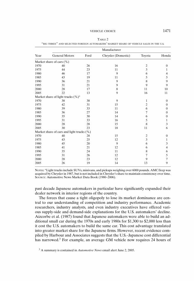
The domestic industry’s loss in market share is not attributable to the problemsexperienced by any one automaker (Table 2). Indeed, GM, Ford, and Chrysler areall losing market share at the same time. Toyota has recently surpassed Ford as

∗ Manuscript received July 2005; revised February 2006.1 We are grateful to S. Berry, F. Mannering, C. Manski, D. McFadden, A. Pakes, P. Reiss, J. Rust, M.

Trajtenberg, F. Wolak, and seminar participants at Berkeley, Maryland, Stanford, UC Irvine, and Yalefor helpful comments. A. Langer provided valuable research assistance. Please address correspondenceto: Kenneth E. Train, Department of Economics, 549 Evans Hall #3880, University of California, Berke-ley, CA 94720-3880, U.S.A. Phone: 415-291-1023. Fax: 415-291-1020. E-mail: [email protected].

2 Ford and General Motors have partial ownership of some foreign automakers. However, theindustry and manufacturer shares reported here would not be affected very much if Ford’s and GM’ssales included, on the basis of their ownership shares, the sales of these automakers.

1469

1470 TRAIN AND WINSTON

TABLE 1U.S. AND FOREIGN AUTOMAKERS’ MARKET SHARE OF VEHICLE SALES IN THE UNITED STATES∗

Manufacturer by Geographic Origin

Year U.S. Japan Europe

Market share of cars (%)1970 86 3 81975 82 9 71980 74 20 61985 75 20 51990 67 30 51995 61 31 52000 53 32 112005 42 40 11Market share of light trucks (%)∗∗1970 91 4 41975 93 6 11980 87 11 21985 81 18 01990 84 16 01995 87 13 02000 77 19 12005 70 25 3Market share of cars and light trucks (%)1970 87 4 71975 85 8 61980 77 18 61985 77 19 41990 72 24 31995 72 23 32000 66 26 62005 57 32 7

NOTES: ∗Shares generally do not sum to 100 because of rounding, the omission of Korean manufacturers,and imports that Automotive News does not assign to any manufacturer or country of origin.∗∗Light trucks include SUVs, minivans, and pickups weighing over 6000 pounds.SOURCE: Automotive News Market Data Book (1980–2006).

the second largest seller of new cars in the United States and Honda has surpassedChrysler (notwithstanding Chrysler’s merger with Daimler-Benz in 1998) and iswithin reach of Ford. Both companies as well as Nissan (not shown) are also likelyto increase their share of the light truck market as their new offerings becomeavailable. On the other hand, General Motors’ share of new car and light trucksales has not been so low since the 1920s.

It may be believed that the industry’s losses in share are confined to certaingeographical regions of the country such as parts of the East and West Coastsand some affluent areas in the Southwest. However, Japanese and European au-tomakers have built manufacturing plants and research and development facilitiesin the mid-West and mid-South that have spurred local employment and helpedincrease market share in these areas because American consumers no longer viewauto “imports” as costing themselves or their friends a job. In addition, during the

VEHICLE CHOICE 1471

TABLE 2“BIG THREE” AND SELECTED FOREIGN AUTOMAKERS’ MARKET SHARE OF VEHICLE SALES IN THE U.S.

Manufacturer

Year General Motors Ford Chrysler (Domestic) Toyota Honda

Market share of cars (%)1970 40 26 16 2 01975 44 23 11 3 11980 46 17 9 6 41985 43 19 11 5 51990 36 21 9 8 91995 31 21 9 9 92000 28 17 8 11 102005 22 13 9 16 11Market share of light trucks (%)∗1970 38 38 9 1 01975 42 31 15 2 01980 39 33 11 6 01985 36 27 14 7 01990 35 30 14 6 01995 31 33 16 5 12000 28 28 15 8 32005 30 23 18 11 6Market share of cars and light trucks (%)1970 40 28 15 2 01975 43 25 12 3 11980 45 20 9 6 31985 41 21 12 6 41990 35 24 11 8 61995 31 26 12 7 52000 28 23 12 9 72005 26 19 14 13 9

NOTES: ∗Light trucks include SUVs, minivans, and pickups weighing over 6000 pounds. AMC/Jeep wasacquired by Chrysler in 1987, but is not included in Chrysler’s share to maintain consistency over time.SOURCE: Automotive News Market Data Book (1980–2006).

past decade Japanese automakers in particular have significantly expanded theirdealer network in interior regions of the country.

The forces that cause a tight oligopoly to lose its market dominance are cen-tral to our understanding of competition and industry performance. Academicresearchers, industry analysts, and even industry executives have offered vari-ous supply-side and demand-side explanations for the U.S. automakers’ decline.Aizcorbe et al. (1987) found that Japanese automakers were able to build an ad-ditional small car during the 1970s and early 1980s for $1,300 to $2,000 less thanit cost the U.S. automakers to build the same car. This cost advantage translatedinto greater market share for the Japanese firms. However, recent evidence com-piled by Harbour and Associates suggests that the U.S.–Japanese cost differentialhas narrowed.3 For example, an average GM vehicle now requires 24 hours of

3 A summary is contained in Automotive News email alert June 2, 2005.


assembly time whereas an average Honda North American vehicle requires 22.3hours. Compared with Japanese transplants, American plants have also signifi-cantly reduced the labor that they require to build a car.

Recently, industry executives such as Bill Ford of Ford and Rick Wagoner ofGeneral Motors have argued that their competitive position has been eroded byrising health care and pension costs and an undervalued yen. They have calledon the federal government to provide the industry with various subsidies and taxbreaks and to pressure Japan to raise the value of its currency. However, the U.S.industry’s market share was declining long before it began to incur the costs of anaging workforce and has continued to decline during times when the dollar/yenexchange rate was quite favorable for U.S. automakers.

From a consumer’s perspective, Japanese automakers have developed a reputa-tion for building high-quality products that suggests that their technology in carsrepresents better value than American technology in cars. Indeed, using variousmeasures of quality and reliability, widely cited publications such as ConsumerReports and the J.D. Power Report have generally given their highest ratings inthe past few decades to cars made by Japanese and European manufacturers in-stead of American manufacturers. Changes in market share since the 1970s couldtherefore be explained by the relative value of the technology in domestic andforeign producers’ vehicles as captured in basic vehicle attributes such as price,fuel economy, power, and so on.

Consumers’ preferences may also be affected by more subtle attributes of avehicle such as the feel of a stereo knob and the shine of plastics used in interiors.Robert Lutz, General Motors’ vice chairman for product development, claimsthat attention to these subtle attributes sends a powerful message to consumersthat an automaker cares about its products.4 An even more subtle considerationis consumers’ unobserved tastes that are expressed, as John DeLorean colorfullyput it, in whether their eyes light up when they walk through an automaker’sshowroom and whether they buy a car that they are in love with.5 U.S. automakersmay have lost market share because of the poor workmanship of their productsor factors that although difficult to quantify have adversely influenced consumers’tastes toward domestic vehicles.

Brand loyalty is inextricably related to developing, maintaining, and protectingmarket share. Mannering and Winston (1991) found that a significant fraction ofGM’s loss in market share during the 1980s could be explained by the strongerbrand loyalty that American consumers developed toward Japanese producers’vehicles compared with the loyalty that they had for American producers’ vehi-cles. Ford and Chrysler were able to retain their share during that period, butthe American firms’ subsequent losses in share may be partly attributable to theintensity of consumer loyalty toward Japanese and European automakers.

Economic theory suggests that product line rivalry may be an important featureof competition in the passenger-vehicle market because consumers have strongly

4 Danny Hakim, “G.M. Executive Preaches: Sweat the Smallest Details,” New York Times, January5, 2004.

5 Danny Hakim, “Detroit’s New Crisis Could Be its Worst,” New York Times, March 27, 2005.

VEHICLE CHOICE 1473

varying preferences. Industry analysts stress that it is important for automakers todevelop attractive product lines that anticipate and respond quickly to changes inconsumer preferences. General Motors, for example, has offered an assortmentof vehicles that missed major trends such as the growth in the small-car market inthe late 1970s and early 1980s, the interest in more aerodynamic midsize cars inthe late 1980s, and the rise of sport utility vehicles based on pickup truck designsin the 1990s. Two key features of an automaker’s product line are the range ofvehicles that are offered and whether any particular vehicle generates “buzz”that spurs sales of all of the automaker’s vehicles. Finally, the competitiveness ofa product line is also affected by an automaker’s network of dealers. Changesin market share since the 1970s could therefore reflect the relative strengths ofdomestic and foreign manufacturers’ product lines and distribution systems.

Given the myriad of hypotheses that have been offered, it is useful to empiri-cally assess as many of them as possible. This article develops a model of consumervehicle choice to investigate the major potential causes of the domestic industry’sshrinking market share. A long line of research beginning with Lave and Train(1979), Manski and Sherman (1980), Mannering and Winston (1985), and Train(1986) indicates that such models are a natural way to quantify a variety of influ-ences on consumers’ behavior, some of which may prove useful for understandingthe industry’s decline. However, these models have accumulated several specifica-tion and estimation concerns including the independence of irrelevant alternatives(IIA) assumption maintained by the multinomial logit model that is often usedto analyze choices, the possibility that vehicle price is endogenous because it isrelated to unobserved vehicle attributes, the importance of accounting for het-erogeneity among vehicle consumers, and the appropriate treatment of dynamicinfluences on choice such as brand loyalty.

We explore these concerns in the process of estimating the choices of U.S. con-sumers who acquired new vehicles in 2000. Although we do not claim to providedefinitive solutions to all of the methodological issues that we confront, we do ob-tain plausible evidence that choices are strongly influenced by vehicle attributes,brand loyalty, and automobile dealerships but surprisingly they are not affectedby product line characteristics. We use the choice model to simulate market sharesunder alternative scenarios to explore the reasons for the loss in market share byU.S. manufacturers.

We find that the U.S. industry’s loss in share during the past decade can beexplained almost entirely by relative changes in the most basic attributes of newvehicles, namely, price, size, power, operating cost, transmission type, reliability,and body type. The result is surprising in its simplicity, implying that it is notnecessary to resort to the plethora of explanations just described. Argumentsbased on subtle attributes such as the design of interior features, unobservedresponses by consumers to vehicle offerings, or even measurable attributes beyondthose listed above do not play a measurable role in the industry’s competitiveproblems. Similarly, changes in loyalty patterns, whether an automaker’s productline is broad or narrow or includes a hot car, and changes in dealership networksdo not contribute much to the industry’s decline. Our finding suggests that U.S.automobile executives should focus more attention on understanding why their


companies seem unable to improve the basic attributes of their vehicles as rapidlyas their foreign competitors are able to improve their vehicles’ basic attributes,and try to remedy the situation.

2. CHOICE OF MODEL AND ITS FORMULATION

Our objective is to investigate the most likely determinants of market sharechanges in the new vehicle market during the past decade. The approach we takeis to estimate the conditional choice of buying a new car. In a complete vehiclechoice model, consumers can choose to buy a new car, buy any used car, continueusing their current vehicles, or not own any vehicle and presumably rely on pubictransportation. Our model, which accounts for unobserved taste variation and isconditional on a subset of the vehicle choice alternatives (i.e., new car purchases),could yield inconsistent estimates if tastes that affect which new car the consumerchooses also affect whether the consumer chooses one of these cars instead ofanother alternative. It is thus useful to discuss the advantages and drawbacksof different approaches to analyzing new vehicle choices before formulating ourmodel.

2.1. Controlling for Related Choices. One approach to the problem of relatedchoices that is taken, for example, by Berry et al. (2004), is to aggregate all theother alternatives into one alternative—which is often called an outside good. Theweakness of this approach is that it is difficult to specify attributes that meaning-fully represent this alternative. Thus, including an outside good is still likely toyield inconsistent estimates because unobserved tastes that affect a consumer’sassessment of new cars can also affect a consumer’s assessment of other alter-natives through the attributes of those alternatives. For example, the value thatconsumers place on vehicle price affects their evaluation of each used car basedon a used car’s price, not just on the existence of an unspecified outside good.6

A further difficulty with using an outside good is that the sample of new carbuyers needs to be weighted to be consistent with the general population. Theseweights differ greatly over observations, because the subpopulation of new carbuyers is quite different from the general population. Thus, the density of tastesamong the subpopulation of new vehicle buyers is derived as being proportionalto the population density times the probability of a buying a new car. But thisprobability is influenced by the attributes of other alternatives including but notlimited to all used and currently owned vehicles. However, as noted, an outsidegood does not control for these attributes; hence, the conditional density is likelyto be incorrectly inferred from the population density.

In our view, the distribution of preferences among new car buyers can be es-timated more accurately by estimating it directly on a sample of new car buyers

6 The utility of the outside good is usually specified as a function of demographic characteristicsand random terms. Although these elements tend to have significant effects, indicating that they arecapturing differences between people who buy the good and those who do not, the utility of the outsidegood is not structural because it does not relate to the attributes of the alternatives that are subsumedinto the aggregate “outside good.”

VEHICLE CHOICE 1475

and by conducting extensive tests of error components that capture vehicle at-tributes and socioeconomic variables that are likely to affect consumers’ newvehicle choices as well as their related choices. Our approach also has the prac-tical advantage that it can include explanatory variables whose distributions arenot known for the general population. In contrast, the outside good approach re-stricts the set of explanatory variables to those whose distributions in the U.S.population are known, because the population distribution is used to weightthe sample. Thus, we would be precluded from exploring, among other influ-ences, the impact of brand loyalty and an automaker’s network on vehicle choicebecause measures of these effects are very difficult to obtain for the generalpopulation.7

Of course, the issues raised here could potentially be avoided by analyzing acomplete model of vehicle ownership. The problems posed by this approach arecost and empirical tractability. As noted later, we must conduct a customizedsurvey of households to collect information on such variables as past vehicle pur-chases, vehicles seriously considered when selecting a new vehicle, and so on.This information is not included in publicly available surveys. Customized surveysare expensive—in our case, the cost was roughly $50 per household. Householdsthat actually acquire a new vehicle represent roughly 12% of the general pop-ulation of households. Thus, the cost of assembling a sample of all householdsin the population, which would be necessary to analyze the choice of whether aconsumer decides to acquire a vehicle, would run into the hundreds of thousandsof dollars. For those households who actually purchase a vehicle, we would haveto analyze whether they selected a new or used vehicle, which would result inan enormous choice set that could not be reduced because our model does notinvoke the IIA assumption. Finally, even a complete model of vehicle ownershipis open to the criticism that it is conditional on other related decisions such asmode choice to work and residential location. Using our approach as a start-ing point, future research can consider the trade-off between additional modelingand costly data collection and possible improvements in the accuracy of parameterestimates.

2.2. Model Formulation. Our analysis is based on a random utility functionthat characterizes consumers’ choices of new vehicles by make (e.g., Toyota)and model (e.g., Camry). A mixed logit model relates this choice to the averageutility of each make and model (i.e., average over consumers), the variation in util-ity that relates to consumers’ observed characteristics, and the variation in utilitythat is purely random and does not relate to observed consumer characteristics.In an auxiliary regression equation, the average utility of each make and modelis related to the observed attributes of the vehicle, using an estimation procedurethat accounts for the possible endogeneity of vehicle prices.

7 By conditioning choices on the purchase of a new vehicle, we are precluded from analyzing orforecasting changes in market size. However, we are interested in decomposing potential influenceson changes in market shares, especially the decline in the U.S. manufacturers’ share. We can conductthis analysis without having to control for changes in market size.


We index consumers by n = 1, . . . , N, and the available makes and models ofnew vehicles by j = 1, . . . , J. The utility, Unj, that consumer n derives from vehiclej is given by

Unj = δ j + β ′xnj + µ′nwnj + εnj ,(1)

where δ j is “average” utility (or, more precisely, the portion of utility that is thesame for all consumers8), xnj is a vector of consumer characteristics interactedwith vehicle attributes, product line and distribution variables, and brand loyalties(capturing observed heterogeneity); β represents the mean coefficient for each ofthese variables in the population; wnj is a vector of vehicle attributes that may beinteracted with consumer characteristics (capturing unobserved heterogeneity);µn is a vector of random terms with zero mean that corresponds to vector elementsin wnj; and εnj is a random scalar that captures all remaining elements of utilityprovided by vehicle j to consumer n.

Brownstone and Train (1999) point out that the terms µ′nwnj represent ran-

dom coefficients and/or error components. Each term in µ′nwnj is an unobserved

component of utility that induces correlation and nonproportional substitutionbetween vehicles, thus overcoming the IIA restriction imposed by the standardlogit model. Note that elements of wnj can correspond to an element of xnj, inwhich case the corresponding element of β represents the average coefficient andthe corresponding element of µn captures random variation around this average.Elements of wnj that do not correspond to elements of xnj can be interpreted ascapturing a random coefficient with zero mean.

Denote the density of µn as f (µ | σ ), which depends on parameters σ thatrepresent, for example, the covariance of µn. Note that f is the density conditionalon a new vehicle purchase and may therefore depend on observed variables in themodel that arise from a consumer’s optimizing behavior that leads to a new vehiclepurchase. We explore the empirical form of f and its dependence on observedvariables as part of our estimation.

We assume that εnj is i.i.d. extreme value. Note that the average utility associatedwith omitted attributes, which varies over vehicles, is absorbed into δ j . Giventhe distributional assumption on εnj , the probability that consumer n choosesalternative i is given by the mixed logit model (see, e.g., Revelt and Train, 1998;McFadden and Train, 2000): 9

Pni =∫

eδi +β ′xni +µ′wni∑j eδ j +β ′xnj +µ′wnj

f (µ | σ ) dµ.(2)

8 The explanatory variables xnj have nonzero mean in general, thus average utility is actually δ j

plus the mean of β ′xnj. We use the term “average utility” to refer to δj because other terms, such as“common utility” or “fixed portion of utility,” seem less intuitive. The main point is that δ j does notvary over consumers whereas the other portions of utility do.

9 These references are for mixed logits on consumer-level choice data. Mixed logits on marketshare data have been estimated by Boyd and Mellman (1980), Cardell et al. (1980), and more recentlyrevived by Berry et al. (1995).

VEHICLE CHOICE 1477

McFadden and Train (2000) demonstrate that by making an appropriate choiceof variables and mixing distribution, a model taking this form can approximateany random utility model—and pattern of vehicle substitution—to any level ofaccuracy.

Market (or aggregate) demand is the sum of individual consumers’ demand. Thetrue (observed) share of consumers buying vehicle i is Si. As in Berry et al. (2004)and Goolsbee and Petrin (2004), we use market shares instead of sample sharesto avoid the sampling variance associated with the latter shares. The predictedshare, denoted Si (θ, δ), is obtained by calculating Pni with parameters θ = {β,σ}and δ = {δ1, . . . , δJ } and averaging Pni over the N consumers in the sample. Berry(1994) has shown that for any value of θ , a unique δ exists such that the predictedmarket shares equal the actual market shares. This fact allows δ to be expressedas a function of θ , thereby reducing the number of parameters that enter thelikelihood function. We denote δ(θ ,S), where S = {S1, . . . , SJ }, as satisfying therelation

Si =Si (θ, δ(θ, S)) =∑

n

Pni (θ, δ(θ, S))/N i = 1, . . . , J.(3)

The parameters of the choice model θ are estimated by maximum likelihoodprocedures described below, and δ is calculated such that predicted market sharesmatch observed market shares at θ .

The alternative-specific constant for each vehicle, δ j (θ , S), captures the averageutility associated with observed as well as unobserved attributes, whereas thevariables that enter the random utility model capture the variation of utility amongconsumers. To complete the model, we specify average utility as a function ofvehicle attributes, z, with parameters, α, that do not vary over consumers:

δ j (θ, S) = α′zj + ξ j ,(4)

where ξ j captures the average utility associated with omitted vehicle attributes.Note that elements of wnj in the random utility function given in Equation (1) cancorrespond to an element of zj.

Vehicle price, an element of zj, is likely to be affected by unobserved attributes,so that ξ j does not have a zero mean conditional on zj. To address this problem, letyj be a vector of instruments that includes the nonprice elements of zj plus otherexogenous variables that we discuss below. The assumption that E(ξ j | yj ) = 0 forall j is sufficient for the instrumental variables estimator of α to be consistent andasymptotically normal, given θ .

3. ESTIMATION PROCEDURES

Estimation of the random utility function presented here is complicated by ourefforts to capture preference heterogeneity (i.e., σ ), the average utility for eachmake and model (i.e., δ), and the effect of brand loyalty on vehicle choice. Wediscuss each of these issues in turn.


3.1. Preference Heterogeneity and Vehicles Considered. The set of vehiclesthat consumers consider before making a purchase provides additional informa-tion on their tastes that may be useful in identifying preference heterogeneity.We therefore asked consumers in our sample to list the vehicles that they seri-ously considered in addition to the vehicle that they purchased. Most consumersindicated that they considered only one vehicle besides their chosen vehicle; noconsumer listed more than five vehicles.

We included this information in estimating the choice model by treating thechosen vehicle and the vehicles that were seriously considered as constitutinga ranking. Consumers who indicated only one “considered” vehicle generated autility ranking of Uni > Unh > Unj for all j = i , h for chosen vehicle i and consideredvehicle h. Consumers who indicated more than one considered vehicle generateda utility ranking in the order that they listed the vehicles.

Luce and Suppes (1965) demonstrated that when the unobserved componentof utility is i.i.d. extreme value, the probability of a utility ranking, starting withthe first-ranked alternative, is a product of logit formulas. Therefore, conditionalon µn, the probability,L n(µn), that a consumer buys vehicle i and also consideredvehicle h is

Ln(µn) =(

eδi (θ,S)+β ′xni +µ′nwni∑J

j=1 eδ j (θ,S)+β ′xnj +µ′nwnj

) (eδh(θ,S)+β ′xnh+µ′

nwnh∑Jj=1, j =i eδ j (θ,S)+β ′xnj +µ′

nwnj

),(5)

where the sum in the second logit formula is over all vehicles except i. The prob-ability of the consumer’s ranking conditional on µn is defined analogously forconsumers who listed more than one considered vehicle. The unconditional prob-ability of the consumer’s ranking is then

Rn =∫

Ln (µ) f (µ | σ ) dµ.(6)

We found in preliminary estimations that it was essential to include the vehiclesthat consumers considered to estimate the distribution of their tastes. When weincluded only the choice of the vehicle that consumers purchased, the parametersof the systematic part of the model were hardly affected but we were unableto obtain any statistically significant error components. In contrast, the standarddeviations for several elements ofµn were found to be significant when we includedthe vehicles that consumers seriously considered. Berry et al. (2004) also reportedthat they were unable to estimate unobserved taste variation without includingconsumers’ rankings.

3.2. Average Preferences. We included dummy variables for all the makes andmodels in our sample to estimate consumers’ average value of utility from eachvehicle. In the numerical search for the maximum of the likelihood function (seebelow), δ is calculated for each trial value of θ . We use the contraction proceduredeveloped by Berry et al. (1995) where at any given value of θ , the following

VEHICLE CHOICE 1479

formula is applied iteratively until predicted shares equal observed market shares(within a given tolerance):

δtj (θ, S) = δt−1

j (θ, S) + ln(Sj ) − ln(S j (θ, δt−1(θ, S))) j = 1, . . . , J.(7)

As in previous applications of this procedure, we found that the algorithm attainsconvergence quickly.

3.3. Brand Loyalty. Brand loyalty has been a crucial consideration in au-tomobile demand analysis beginning with Manski and Sherman (1980), who in-cluded a transactions dummy variable in their vehicle choice model, Manneringand Winston (1985), who included lagged utilization variables, and Mannering andWinston (1991), who included “brand loyalty” variables defined as the number ofprevious consecutive purchases from the same manufacturer. We use the last mea-sure of brand loyalty here. The notion of brand loyalty suggests that householdsmay behave myopically with respect to their vehicle ownership decisions—thatis, they do not take full account of the impact of their present consumption ofautomobiles on future tastes. Indeed, households do appear to behave myopicallyas indicated by high implicit discount rates based on vehicle purchase decisions(Mannering and Winston, 1985) and by frequent breaks in loyalty. Accordingly,researchers have not modeled consumers’ vehicle choices as arising from the max-imization of an intertemporal utility function subject to an intertemporal budgetconstraint.

We specify separate brand loyalty variables in our model for GM, Ford, Chrysler,Japanese manufacturers as a group, European manufacturers as a group, and Ko-rean manufacturers as a group. However, care must be taken when interpretingthese coefficients (Mannering and Winston, 1991). One interpretation, which isbased on the idea of state dependence that we are attempting to capture, positsthat a consumer’s ownership experience with a manufacturer’s products buildsconfidence in that manufacturer (e.g., reduces perceived risk) thereby producinga greater likelihood that a consumer will buy the manufacturer’s products in the fu-ture. Consumers’ actual experiences with a manufacturer’s vehicles determine theintensity of their loyalty—positive experiences are reflected in a large coefficientfor the manufacturer’s loyalty variable. An alternative interpretation is that theloyalty variable captures unobserved taste heterogeneity among consumers that isnot controlled for elsewhere in the model: Previous purchases reflect consumers’tastes that influence their current purchase.

As Heckman (1991) pointed out, state dependence and consumer heterogeneityare fundamentally indistinguishable unless one imposes some structure on the wayobserved and unobserved variables interact. In our case, we contend that it is morelikely that brand loyalty is capturing state dependence instead of heterogeneitybecause it is defined for manufacturers that produce a wide range of vehicles,especially when Japanese and European vehicles are each considered as a group.Unobserved heterogeneity is more likely to be associated with makes and modelsthan with manufacturers. For example, if a middle-aged male bought a Honda


S2000 in the past because it best matched his tastes, then, based on his revealedtastes, it is reasonable to expect that he would be more likely to buy a PorscheBoxer or a Mercedes SLK in his current choice than to buy a Honda Accord orToyota Camry.

Our brand loyalty variables could nevertheless be subject to endogeneity biasto the extent that they relate to unobserved tastes for vehicle attributes; that is,the distribution of random terms in the choice model may be different condi-tional on different values of the brand loyalty variables. Heckman (1981a, 1981b)pioneered the development of dynamic discrete choice models with lagged depen-dent variables and serially correlated errors, recognizing the critical role of initialconditions. However, applying his methods to address the possible bias of brandloyalty coefficients is thwarted by formidable data and computational require-ments. First, we would have to obtain data for all sampled consumers indicatingtheir vehicle choices and the attributes of the vehicles that were available at thetime of each previous purchase beginning with the first vehicle that they ever pur-chased. Second, we would have to simultaneously estimate previous and currentvehicle choice probabilities incorporating these data and a plausible specificationof how consumers’ tastes are likely to change over time.

We therefore take a simpler and more tractable approach that, although notnecessarily leading to a consistent stochastic structure, can be expected to capturethe primary differences in the error distribution of the random utility functionconditional on our brand loyalty variables. As reported later, we also estimatethe model without any loyalty variables and find that the estimates for all otherparameters are nearly the same with and without the loyalty variables. Hence,any inconsistency that is induced by the loyalty variables and our treatment ofthe conditional error distribution is confined to the loyalty parameters themselvesand does not affect other parameters.

We represent the information contained in the loyalty variables about con-sumers’ preferences across manufacturers by denoting each consumer’s man-ufacturer preference as ηnm, with m = 1, . . . , 6 indexing the six manufacturergroups (GM, Ford, Chrysler, Japanese, European, and Korean.) These prefer-ences result from the manufacturers’ offerings and consumers’ tastes for thevehicles’ attributes. In the past, consumer n chose the manufacturer with the high-est value of ηnm. The unconditional distribution of ηn = {ηn1, . . . , ηn6} is g(ηn).The distribution of ηn conditional on the consumer having chosen manufacturerm is

h(ηn | ηnm > ηns∀s = m) = I(ηnm > ηns∀s = m)g(ηn)∫I(ηnm > ηns∀s = m)g(ηn)dηn

,(8)

where I(·) is a 0–1 indicator of whether the statement in parentheses is true.For the current choice, the utility of vehicle j, which is produced by manufac-

turer s(j), is as previously specified plus a term ληns , where λ is the coefficientof the additional element of utility. Conditional on the past choice of manufac-turer, the choice probability is then the logit formula with this term added to itsargument, integrated over the conditional density of ηn. Formally, the probability

VEHICLE CHOICE 1481

that consumer n chooses vehicle i produced by manufacturer s(i), given that theconsumer chose a vehicle by manufacturer m in the past (where m may equal s(i))is:

Pni =∫∫

eδi +β ′xni +µ′nwni +ληns(i)∑J

j=1 eδ j +β ′xnj +µ′nwnj +ληns( j)

× f (µ | σ )h(ηn | ηnm > ηns∀s = m) dµdηn.(9)

This choice probability is a mixed logit with an extra error component whosedistribution is conditioned on the consumer’s past choice of manufacturer. Sim-ilarly, the probability for the observed choices of consumer n, who for instancebought vehicle i and ranked vehicle h as second, is the same as Equation (5) butexpanded to include the extra error component

Rn =∫∫

eδi +β ′xni +µ′nwni +ληns(i)∑J

j=1 eδ j +β ′xnj +µ′wnj +ληns( j)

× eδh+β ′xnh+µ′nwnh+ληns(h)∑J

j =i, j=1 eδ j +β ′xnj +µ′wnj +ληns( j)f (µ | σ )h(ηn | ηnm > ηns∀s = m) dµdηn.

(10)

Note we also account for additional ranked choices as appropriate.

3.4. Estimators. The choice probabilities,Pni, in Equation (9) and the rankingprobabilities, Rn, in Equation (10), are integrals with no closed form solution. Weuse simulation to approximate the integrals. The simulated choice probability is

Pni = 1D

D∑d=1

eδi (θ,S)+β ′xni +µ′dwni +ληrdns(i)∑

j eδ j (θ,S)+β ′xnj +µ′dwnj +ληrdns( j)

,(11)

for draws µd, d = 1, . . . , D from density f (µ | σ ) and draws from the conditionaldistribution h. The probability of consumer n’s purchased and ranked vehicles aresimulated similarly, giving Rn.

The simulated log-likelihood function for the observed first and ranked choicesin the sample is LL = ∑

n lnRn, which is maximized with respect to parametersθ = {β,σ} and λ. As described above, estimates of δ = {δ1, . . . , δJ } are obtainedusing the iteration formula in Equation (7) to ensure that predicted shares equalobserved market shares.10 Goolsbee and Petrin (2004) also use maximum likeli-hood procedures to estimate choice probabilities. Petrin (2002) and Berry et al.

10 Our sample size is small relative to the number of available makes and models, and thus relativeto the number of elements in δ. However, this is not problematic because observed market sharesrather than sample shares are used to determine δ. Note that the sample of new vehicle buyers is largerelative to the number of elements in θ that reflect differences in preferences among households, andit is this sample that is used to estimate θ .


(2004) used a generalized method of moments estimator with moments based onconsumer-level choices.

We use 200 Halton draws for simulation.11 Halton draws are a type of low-discrepancy sequence that, as R rises, has coverage properties that are superiorto pseudo-random draws. For example, Bhat (2001) and Train (2000) found that100 Halton draws achieved greater accuracy in mixed logit estimations than 1,000pseudo-random draws.12 To estimate the impact of different numbers of draws onparameter estimates, we estimated the model using 100, 150, and 200 draws. Theestimates differed an average of 8% when we increased the number of draws from100 to 150 and differed an average of 4% when we increased the number of drawsfrom 150 to 200. The differences are well within the confidence intervals for theparameters and indicate that simulation noise and bias are sufficiently small to notwarrant further increases in the number of draws. In addition, we evaluated thelog-likelihood function, gradient, and Hessian using 400 draws at the parameterestimates obtained with 200 draws. The average log-likehood changed only veryslightly, from –6.5163 to –6.5141. The test statistic g′H−1g, where g is the gradientvector and H is the Hessian, took the value 0.00351. Under the null hypothesisthat the gradient is zero, this test statistic is distributed chi-squared with degreesof freedom equal to the number of parameters. The extremely low value indicatesthat we cannot reject the hypothesis that the gradient using 400 draws is zero at theestimates using 200 draws at any meaningful level of significance. For these reasons,we concluded that using 200 Halton draws for simulation was sufficient. We reportrobust standard errors that take into account simulation noise, as suggested byMcFadden and Train (2000).

After estimating the ranked choice probabilities, we estimate the regressiongiven by Equation (4), which relates the alternative-specific constants that captureaverage utilities to vehicle attributes. As noted, we use instrumental variablesbecause price is likely to be correlated with omitted attributes. Nash equilibriumin prices implies that the price of each vehicle depends on the attributes of all theother vehicles, which indicates that appropriate instruments can be constructedfrom these attributes because they are unlikely to be correlated with a givenvehicle’s omitted attributes. Letting dji be the difference in an attribute, say fueleconomy, between vehicle j and i, we calculate four instruments for vehicle i foreach attribute: the sum of dji over all j made by the same manufacturer, the sum of

11 Draws from the conditional distribution h were obtained by an accept/reject procedure: drawvalues of ηn from g(ηn) and retain those for which ηnm > ηns for all s = m. We assume g(ηn) is aproduct of standard normal variables and use 200 accepted draws in the simulation of the integral overηn.

12 Other forms of quasi-random draws have been investigated for use in maximum simulated likeli-hood estimation of choice models. Sandor and Train (2004) explore (t,m,s)-nets, which include Sobol,Faure, Niederreiter, and other sequences. They find that Halton draws performed marginally betterthan two types of nets and marginally worse than two others, and that all the quasi-random methodsvastly outperformed pseudo-random draws. In high dimensions, when Halton draws tend to be highlycorrelated over dimensions, Bhat (2003) has investigated the use of scrambled Halton draws, and Hesset al. (2006) propose modified Latin hypercube sampling procedures. The dimension of integration inour model is not sufficiently high to require these procedures.

VEHICLE CHOICE 1483

dji over all j made by competing manufacturers, the sum of d2j i over all j made by

the same manufacturer, and the sum of d2j i over all j by competing manufacturers.

The four measures are the instruments obtained from the exchangeable basisdeveloped by Pakes (1994). The first two have been used by Berry et al. (1995)and Petrin (2002). The latter two measures, which have not been used before,capture the extent to which other vehicles’ nonprice attributes differ from vehiclei’s nonprice attributes. We found them to be quite useful in our estimations be-cause without them parameter estimates tended to be less stable across alternativespecifications.

Estimation of the first stage regressions for price and retained value (the two en-dogenous variables described further below) obtained R2 of 0.82 and 0.83, respec-tively. Based on F-tests, the hypotheses that all instruments have zero coefficientsand that the extra instruments that do not also enter as explanatory variables inthe second stage have zero coefficients, can be rejected at the 99% confidencelevel. We should point out, however, that use of the instruments assumes thatunobserved attributes, although correlated with price, are independent of the ob-served nonprice attributes of vehicles. This assumption, previously maintained byBerry et al. (1995, 2004) and Petrin (2002), is justified to some extent by pragmaticconsiderations. In future work, it would be useful to explore the possibility of andremedies to any endogeneity in observed nonprice attributes.

4. MODEL SPECIFICATION, DATA, AND ESTIMATION RESULTS

The random utility function in Equation (1) posits that consumers’ vehiclechoices and their ranking of vehicles that they seriously considered are deter-mined by vehicle attributes, their socioeconomic characteristics and brand loyalty,and an automaker’s product line and distribution network. The regression modelspecifies the average utility of a given make and model as a function of vehicleattributes.

In addition to a vehicle’s purchase price, the attributes that we include in themodels are fuel economy, horsepower, curb weight, length, wheelbase, reliability,transmission type, and size classifications. These attributes encompass those usedin previous research. Other safety-related variables such as airbags and antilockbrakes were not included because most vehicles in our sample were equipped withthem. Because automobiles are a capital good, consumers’ choices may also beinfluenced by their expectations of how much a vehicle’s value will depreciate. Wetherefore include as a separate variable the percentage of a vehicle’s purchase pricein 2000 (consistent with the sample discussed below) that it is expected to retainafter two years of ownership. Calculating the retained value based on three years ofownership produced a slightly worse fit than using two years of ownership, whereascalculating the value based on four years of ownership produced a noticeablyworse fit. We expect that consumers are more likely to select a vehicle that retainsits value (i.e., the coefficient should have a positive sign) because it could be soldor traded in for a higher price than a vehicle that retains little of its value. Asnoted, we measure brand loyalty by a consumer’s consecutive purchases of the


same brand of vehicle. The socioeconomic characteristics that we include are sex,age, income, residential location, and family size.

Our specification extends previous vehicle demand models by exploring the ef-fect of automakers’ product line and distribution network on choice. Researchershave typically used brand preference dummy variables to capture these influences.Economic theory suggests that broad product lines can create first mover advan-tages to a firm and overcome limited information in a market; thus, we specify thenumber of distinct models (i.e., nameplates) offered by an automaker to capturethese possible effects. During the past decade, GM in particular has been criticizedfor offering too many models that are essentially the same vehicle, suggesting thatthe sign of this variable may vary by automaker. Industry analysts stress that au-tomakers benefit from having a “hot car” in their product line because it may drawattention to other vehicles that they produce. For many decades, a well-known ax-iom among the Big Three was: “bring them into the showroom with a convertible,and sell them a station wagon.” Recently, GM tried to get buzz for the PontiacG6 sedan that it hoped would spillover to its other products by giving away 276of these vehicles on Oprah Winfrey’s television show. We constructed a dummyvariable that indicated whether a manufacturer produced a hot car, where a hotcar was defined as having sales equal to the mean sales of its subclass plus twice thestandard deviation of sales. (We also explored other definitions.) An automaker’snetwork of dealers distributes its products to potential customers; thus, we alsoinclude the number of each manufacturing division’s dealerships.

We performed estimations based on a random sample of 458 consumers whoacquired—that is, paid cash, financed, or leased—a new 2000 model year vehicle.13

Although these consumers differed in how they financed a vehicle, we found thattheir choice model parameters were not statistically different and thus combinedthem to estimate a single model. The sample was drawn from a panel of 250,000nationally representative U.S. households that is aligned with demographic datafrom the Current Population Survey of the U.S. Bureau of the Census. The panel isadministered by National Family Opinion, Inc., and managed by Allison-Fisher,Inc. The response rate for our sample exceeded 70%. The data consist of con-sumers’ new vehicle choices by make and model, their ranking of the vehiclesthey seriously considered acquiring, vehicle ownership histories, which are usedto construct the brand loyalty variables, and socioeconomic characteristics. Ve-hicle attributes and product line variables are from issues of Consumer Reports,the Market Data Book published by Automotive News, and Wards’ AutomotiveYearbook. We follow previous research and use the manufacturer suggested re-tail price, MSRP, for the purchase price. Although manufacturers discount theseprices with various incentives, such as cash rebates and interest free loans, dur-ing our sample period the difference between the incentives offered by American,Japanese, and European manufacturers as a percentage of the retail prices of their

13 The sample size is limited by our requiring data for each consumer on the number of dealers within50 miles that sell each make/model of vehicle and consumers’ vehicle ownership histories and rankingsof vehicles they considered in their 2000 choice. This information is not available from standard surveyssuch as the CES. Our survey enabled us to obtain the information, but at a high cost per respondent.

VEHICLE CHOICE 1485

TABLE 3DESCRIPTION OF THE SAMPLE (CONSUMERS WHO ACQUIRED A NEW VEHICLE IN THE YEAR 2000)

Socioeconomic CharacteristicsVariable Sample Value

Average household income $67,767Average age 54.2Percent male 54Percent with child aged 1–16 19Percent who live in rural location∗ 45

Market Share of Cars and Light Trucks by Manufacturer’s Geographic Origin:Manufacturer Share (percent)

U.S. 64Japanese 28European 5Other 3

NOTE: ∗A rural location is defined as being outside of an MSA of 1 million people or more.

vehicles was quite small. Vehicles’ expected retained values were obtained fromthe Kelley Blue Book: Residual Value Guide. The number of division dealershipswithin 50 miles of a respondent’s zip code was obtained from the automakers’websites. A 50-mile radius seems appropriate for our analysis because CNW Mar-keting Research found that consumers travel 22 miles, on average, to acquire anew vehicle. In addition, some automakers’ web pages only display dealershipswithin 50 miles of the inputted zip code.

Table 3 provides some descriptive information about the sample. It is difficult toobtain population data to assess the sample because it is conditional on a consumeracquiring a new 2000 model year vehicle. However, as noted, the sample is derivedfrom a panel of U.S. households whose demographics are consistent with nationalfigures; accordingly, the sample values of the socioeconomic characteristics appearto be representative. Moreover, the sample market shares of the manufacturersby geographic origin are well aligned with the national market shares reported inTable 1.

Each consumer’s choice set consisted of the 200 makes and models of new 2000vehicles. We treated a number of manufacturers that merged in the late 1990s,for example, Daimler-Benz and Chrysler, as offering distinct makes because itwas likely that consumers had not yet perceived that their vehicles were madeby the same manufacturer. Indeed, we obtained more satisfactory statistical fitsunder this assumption than using the merged entity as a unit of analysis. Given thischoice set, we estimated a mixed logit model that included brand loyalty, productline and distribution variables, and vehicle attributes interacted with consumercharacteristics, error components, and an alternative specific constant for eachvehicle make and model. The estimated constants, which capture average utility,were then regressed against vehicle attributes using instrumental variables.

Table 4 presents estimation results for all parts of the model because eachpart contributes to consumers’ utility. The first panel gives coefficients for two


TABLE 4VEHICLE DEMAND MODEL PARAMETER ESTIMATES∗

Average Utility: Elements of α′zj Coefficient (Standard Error)

Constant −7.0318 −6.8520(1.4884) (1.5274)

Manufacturer’s suggested retail price (in thousands of 2000 dollars) −0.0733 −0.1063(0.0192) (0.0635)

Expected retained value after 2 years (in thousands of 2000 dollars) – 0.0550(0.1011)

Horsepower divided by weight (in tons) 0.0328 0.0312(0.0117) (0.0120)

Automatic transmission dummy (1 if automatic transmission is 0.6523 0.6787standard equipment; 0 otherwise) (0.2807) (0.2853)

Wheelbase (inches) 0.0516 0.0509(0.0127) (0.0128)

Length minus wheelbase (inches) 0.0278 0.0279(0.0069) (0.0069)

Fuel consumption (in gallons per mile) −0.0032 −0.0032(0.0023) (0.0023)

Luxury or sports car dummy (1 if vehicle is a luxury or sports car, 0 −0.0686 −0.0558otherwise) (0.2711) (0.2726)

SUV or station wagon dummy (1 if vehicle is a SUV or wagon, 0 0.7535 0.7231otherwise) (0.4253) (0.4298)

Minivan and full-sized van dummy (1 if vehicle is a minivan −1.1230 −1.1288or full-sized van, 0 otherwise) (0.3748) (0.3757)

Pickup truck dummy (1 if the vehicle is a pickup truck, 0 otherwise) 0.0747 0.0661(0.4745) (0.4756)

Chrysler manufacturer dummy 0.0228 0.0654(0.2794) (0.2906)

Ford manufacturer dummy 0.1941 0.2696(0.2808) (0.3060)

General Motors manufacturer dummy 0.3169 0.3715(0.2292) (0.2507)

European manufacturer dummy 2.4643 2.4008(0.3424) (0.3624)

Korean manufacturer dummy 0.7340 0.8017(0.3910) (0.4111)

Utility that Varies over Consumers Related to Observed Characteristics: CoefficientElements of β ′xnj (Standard Error)

Manufacturers’ suggested retail price divided by respondent’s income −1.6025(0.4260)

Vehicle reliability based on the Consumer Reports’ repair index for 0.3949women aged 30 or over (0 otherwise)a (0.0588)

Luxury or sports car dummy for lessors (1 if the vehicle is a luxury or 0.6778sports car and the respondent leased, 0 otherwise) (0.4803)

Minivan and full-sized van dummy for households with an adolescent (1 ifthe vehicle is a van and the respondent’s household has children aged 7 to16, 0 otherwise)

3.2337(0.5018)

SUV or station wagon dummy for households with an adolescent (1 ifvehicle is a SUV or Wagon and the respondent’s household includes achild aged 7 to 16, 0 otherwise)

2.0420(0.4765)

(Continued)

VEHICLE CHOICE 1487

TABLE 5CONTINUED

ln(1+Number of dealerships within 50 miles of the center of a respondent’s zipcode)b

1.4307(0.2714)

Number of previous consecutive GM purchases 0.3724(0.1471)

Number of previous consecutive GM purchases for respondents who live in arural locationc

0.3304(0.2221)

Number of previous consecutive Ford purchases 1.1822(0.1498)

Number of previous consecutive Chrysler purchases 0.9652(0.2010)

Number of previous consecutive Japanese manufacturer purchases 0.7560(0.2255)

Number of previous consecutive European manufacturer purchases 1.7252(0.4657)

Utility that Varies over Consumers Unrelated to Observed Coefficient

Characteristics (Error Components): Elements of µ′nwnj + ληns (Standard Error)

Manufacturer’s suggested retail price divided by respondent’s income times arandom standard normal

0.8602(0.4143)

Horsepower times a random standard normal 45.06(72.34)

Fuel consumption (gallons of gasoline per mile) times a random standard normal −0.0102(0.0020)

Light truck, van, or pickup dummy (1 if vehicle is a light truck, van, or pickuptruck; 0 otherwise) times a random standard normal

6.8505(2.5572)

Manufacturer loyalty: conditional standard normal as described in text. 0.3453(0.1712)

NOTES: ∗Estimated coefficients for vehicle make and model dummies not shown.Number of observations: 458.Log-likelihood at convergence for choice model: −1994.93.R2 for regression model: 0.394 without retained value, 0.395 with retained value.aThe Consumer Reports’ repair index is a measure of reliability that uses integer values from 1 to 5.A measure of 1 indicates the vehicle has a “much below average” repair record, 3 is “average,” and 5represents “much better than average” reliability.bA dealership is defined as a retail location capable of selling a vehicle produced by a given division. Thedealership variable is equal to 0, 1, 2, or 3 (with 3 representing areas with 3 or more dealerships withina 50-mile radius of the center of the respondent’s zip code). This variable is defined for divisions (notmanufacturers), because a Chevrolet dealership might sell Chevrolet vehicles without selling Saturnvehicles (GM manufactures both Chevrolet and Saturn).cA respondent is classified as living in a rural location if he or she does not live in a MetropolitanStatistical Area or lives in a Metropolitan Statistical Area with less than 1 million people.

specifications of average utility; for reasons explained below, one specificationdoes not include the retained value and the other does. The second panel containsthe estimated coefficients for the variation in utility that relates to consumers’observed characteristics; and the third, coefficients for the error components, as-sumed to be normally distributed, that capture variation in utility that is not relatedto observed characteristics. Alternative distributions for the error componentssuch as the lognormal did not produce fits as satisfactory as the normal.


TABLE 5ESTIMATED PRICE COEFFICIENTS AND ELASTICITIES FOR MODELS WITH AND WITHOUT THE RETAINED VALUE

Model without Retained Value Model with Retained Value

OLS IV OLS IV

Purchase price −0.043 −0.073 −0.122 −0.106(0.0094) (0.0192) (0.0362) (0.0635)

Retained value – – 0.130 0.055(0.0577) (0.1011)

Average price elasticity −1.7 −2.3 −3.2 −2.9

4.1. Price Coefficients. Consumers’ response to a change in the price of agiven vehicle is captured by an average effect, an effect that varies with income,and an effect that varies over consumers with the same income. That is, for themodel without retained value, the estimate of the derivative of utility with respectto price is

−0.073 − 1.60/consumer income + 0.86η/consumer income,

where η is distributed standard normal. As previously indicated, the first term isestimated using instrumental variables (IV); when ordinary least squares (OLS) isused the coefficient falls to –0.043 indicating that omitted attributes are correlatedwith price and that it is important to correct for endogeneity in estimation. Basedon these coefficients, the average price elasticity for all vehicles is –2.32, which isconsistent with estimates obtained by Berry et al. (2004).14

When a vehicle’s expected retained value is specified as an additional explana-tory variable, it appears to play an important role in controlling for the endogene-ity of price. We isolate this effect in Table 5, which reports the coefficients for thepurchase price and the retained value estimated by OLS and IV. Given that theretained value is derived from the purchase price, it is likely to be correlated withunobserved attributes of the vehicle and should therefore be estimated by IV. Asnoted, when we include price but not the retained value in the specification, thedifference between the OLS and IV estimates indicated a considerable degree ofendogeneity. But when we also include the retained value, it appears to absorbmost of the endogeneity bias whereas the OLS and IV estimates of the purchaseprice are very similar. This finding suggests that unobserved attributes are corre-lated with a vehicle’s retained value but not with the difference between its priceand retained value (i.e., expected vehicle depreciation).

Note that the retained value represents about 60%, on average, of the purchaseprice (as measured by the MSRP) of a vehicle; thus, the combined effect, regard-less of whether it is estimated by OLS or IV, of the retained value and price on

14 The elasticities are calculated as the percent change in predicted market share that results froma 1% change in price, where predicted market shares are obtained by integrating over both observedand unobserved consumer attributes. A separate elasticity is calculated for each make and model ofvehicle. The average given in the text is over all makes and models.

VEHICLE CHOICE 1489

average utility is roughly the same as the effect of price when it is entered by itself.This relationship suggests that the model with the retained value effectively de-composes the two components of price to which a consumer responds. Moreover,holding retained value constant, Table 5 shows that consumers’ response to price(i.e., the average price elasticity) is clearly higher than when the retained value isallowed to vary. The reason is that the retained value is determined by competitiveused-vehicle markets; hence, if a manufacturer raises the price of a new vehiclewithout improving its attributes, the retained value will not rise proportionatelyand may not rise at all.

As expected, the separate price effects are estimated with less precision thanthe combined effect. Indeed, the estimated coefficient of retained value obtainsa t-statistic of only 0.5, which suggests that the hypothesis that consumers do notdifferentiate between the two components of price cannot be rejected. Nonethe-less, the pattern of estimates is consistent with rational behavior and a plausibleform of endogeneity, and may have important implications for estimating the priceelasticity that is actually relevant to firms’ behavior. It therefore seems reasonableto maintain the concept of retained value as a potential influence among the set ofvehicle attributes affecting consumer choice and subject it to further explorationin future research.15

4.2. Other Coefficients. The nonprice vehicle attributes in Table 4 enter utilitywith plausible signs and are nearly always statistically significant. Vehicle relia-bility, horsepower divided by curb weight, automatic transmission included asstandard equipment, wheelbase, and vehicle length beyond the wheelbase have apositive effect on the likelihood of choosing a given vehicle, while fuel consump-tion per mile (the inverse of miles per gallon) has a negative effect. Note thatwheelbase tends to reflect the size of the passenger compartment and therefore,as expected, has a larger coefficient than vehicle length beyond the wheelbase.Other measures of vehicle size, such as width and a proxy for interior volume,did not have statistically significant effects. We also performed estimations thatincluded engine size (in liters), but it had a statistically insignificant effect.

Our findings that the (dis)utility of price is inversely related to income and thatreliability has a positive and statistically significant effect on utility for womenover 30 years of age but has an insignificant effect for men and for women under30 exemplify observed heterogeneity in consumer preferences. Other examples

15 The inclusion of retained value may alternatively be interpreted as an application of Matzkin’s(2004) method of correcting for endogeneity. Retained value would qualify as the extra variableneeded for Matzkin’s approach if it is related to the price only through exogenous perturbations, but iscorrelated with the unobserved attributes of a vehicle. Under these conditions, the original error termmay be expressed as a function of the retained value and a new error term that is independent of allexplanatory variables including price, which would permit OLS estimation of the regression to yieldconsistent parameter estimates. As expected from an endogeneity correction, the OLS estimate of theprice coefficient rises when the retained value is included in the model (compare the OLS estimatein the third column of Table 5 with the OLS estimate in the first column) and is similar to the IVestimate of the price coefficient (in the second column). We also estimated the function of retainedvalue nonparametrically and obtained essentially the same results as when we specified retained valuelinearly.


are that consumers who lease a vehicle are more likely to engage in upgrade be-havior by choosing a luxury or sports car than consumers who purchase a vehicle(Mannering et al., 2002, discuss this phenomenon), and that households with ado-lescents are more likely than other households to choose a van or SUV presumablyto use for work and nonwork trips.

Unobserved preference heterogeneity is captured in error components relatedto vehicle price, horsepower, fuel consumption, and consumers’ preferences forcars versus trucks (including light trucks, vans, and SUVs).16 The last coefficientreflects greater substitution among cars and among trucks than across these cat-egories, which is confirmed by our estimates of vehicle cross-elasticities. For ex-ample, we find that the cross-elasticity of demand with respect to the price of agiven make and model of a van is, on average, 0.038 for other makes and models ofvans, 0.026 for makes and models of SUVs, 0.018 for makes and models of pickuptrucks, 0.0025 for makes and models of regular cars, and 0.0021 for makes andmodels of sports and luxury vehicles.17 As expected, cross-elasticities are higherfor more similar types of vehicles. We also found reasonable cross-elasticity pat-terns for the prices of other vehicle types. In contrast, a model that maintainedthe IIA property would restrict the cross-elasticity of demand with respect to agiven vehicle’s price to be the same for all vehicles; that is, IIA implies that theelasticity of vehicle j’s demand with respect to a change in vehicle i’s price is thesame for all j = i .

Surprisingly, we found that, all else constant, consumers were not more likelyto purchase a vehicle from automakers that offered a large (or small) number ofmodels or that produced a “hot car.” We explored various definitions of a hotcar to construct its dummy variable, based on deviations from mean sales andsales growth, but they were all statistically insignificant. We also specified hotcar dummies based on vehicle size classifications but they were also statisticallyinsignificant. Although automakers cannot rely on product line “externalities” toimprove their sales, we found that their dealer network does have a statisticallysignificant effect on choice. We constructed the dealership variable by divisionas the natural log of one plus the actual number of dealers within 50 miles ofthe consumer up to a maximum of three. Thus, the variable takes on a value ofzero if no dealers within the circumscribed area sell the vehicle. In addition, thefunctional form assumes that the impact of having one dealer instead of none isgreater than the extra impact of having a second dealer instead of one, and so on,with the impact of additional dealers negligible beyond three. This specification

16 These components were determined after extensive testing of a variety of specifications, includingmodels that allowed the densities to depend on income and other variables. We were not able toidentify any other statistically significant influences on the components beyond those captured in thefixed portion of utility (i.e., the mean of the error components). Recall that we could not identifysignificant error components without including data on considered vehicles, which suggests that thedata contain limited information on the distribution of unobserved taste variation.

17 To put the magnitude of the cross-elasticities in perspective, if a vehicle had a market share of0.005 (i.e., the average share because there are 200 makes and models of vehicles) and had an own-price elasticity of –3.0, then the cross-price elasticity for each other vehicle, assuming it did not vary,would be 0.0151.

VEHICLE CHOICE 1491

fit the data better than a linear specification, indicating that it is important forautomakers to have a dealer within reasonable proximity to potential customersbut that additional dealers will have a diminishing impact on sales.

Finally, we included separate brand loyalty variables for GM, Ford, and Chrysleras well as for the Japanese and European automakers as distinct groups. Prelim-inary estimations indicated that it was statistically justifiable to aggregate theJapanese and European automakers into single loyalty variables. We could notestimate a brand loyalty parameter for Korean automakers because only oneconsumer in the sample chose a Korean vehicle in his or her most recent previ-ous purchase. The estimated coefficients are positive, statistically significant, andfairly large and the error component for brand (manufacturer) loyalty is statisti-cally significant. We found that the likelihood function increased when we usedthe conditional distribution of ηn instead of its unconditional distribution, whichindicates that conditioning provides useful information about consumers’ choices.

When our estimates are assessed in the context of previous findings that usethe same measure of brand loyalty as used here, it becomes clear that loyaltieshave undergone considerable shifts as consumers have gained experience withand adjusted to new information about automakers’ products. Mannering andWinston (1991) found that during the 1970s, American consumers had the greatestbrand loyalty toward Chrysler, had comparable loyalty toward GM and Japaneseautomakers, and the least loyalty for Ford. During the 1980s, after Americanconsumers developed greater experience with Japanese vehicles, Mannering andWinston found that loyalty toward Japanese automakers exceeded loyalty towardany American automaker. But during the mid-1990s, as American consumersgained experience with certain automakers by leasing their vehicles and purchas-ing a greater share of light trucks, Mannering et al. (2002) found that Americanconsumers developed strong brand loyalty toward European automakers and re-vived some of their loyalty toward American firms.

Our brand loyalty estimates indicate that this recent shift is intact becauseconsumers have the strongest loyalty toward European automakers and loyalty forFord and Chrysler now exceeds loyalty toward Japanese automakers. Of course,Ford’s and Chrysler’s loyalty coefficients may indicate that as their market shareshave fallen, they have retained a smaller but more loyal group of customers. GMhas the least loyalty and, in contrast to Ford and Chrysler, appears to be retainingonly loyal rural customers as its share falls.

We stress that our interpretations should be qualified on theoretical groundsbecause the loyalty coefficients could also be capturing heterogeneity in tastes.We cannot resolve the theoretical debate, but we did explore additional empiricaltreatments of brand loyalty to shed light on the validity of our interpretation. Inparticular, if the phenomenon we are capturing were unobserved tastes for vehicletypes, then it is likely that such tastes would be correlated with at least some ofthe vehicle attributes in the model. But, as noted earlier, when we performedestimations without a manufacturer error component and without including thebrand loyalty variables, the other (nonbrand loyalty) parameters were nearly thesame as those presented in Table 4. Of course, this exploration does not rule outthe possibility that the loyalty variables themselves are subject to endogeneity bias;


but at a minimum it indicates that such bias does not affect the other parametersof the model, which is an important consideration when we assess the sources ofchanges in market shares.

5. ASSESSING THE U.S. AUTOMAKERS’ DECLINE

The main purpose of the vehicle choice model is to guide an exploratory as-sessment of the ongoing decline in U.S. automakers’ market share. As discussedin the introduction, several hypotheses that explain the decline could be derivedfrom the academic literature and the views of industry observers and participantsincluding changes in basic vehicle attributes, subtle vehicle attributes, unobservedtastes, brand loyalty, product line characteristics, and distribution outlets.

The findings obtained from the vehicle choice model narrow the range of pos-sible explanations to vehicle attributes and unobserved tastes. The statisticallyinsignificant parameter estimates for the product line variables and the apparentrelative improvement in brand loyalty for Ford and Chrysler suggest that thesefactors are unlikely to have been a major source of the industry’s loss in marketshare. Foreign automakers have improved their distribution networks over time,but U.S. automakers compete effectively in this dimension. Thus, we first focus onthe impact of changes in basic vehicle attributes during the past decade on U.S.automakers’ market shares and if necessary turn to less observable factors.

We use data on the vehicles offered in 1990 and their attributes to forecast thechange in U.S. automakers’ market share attributable to changes in vehicle at-tributes given consumers’ tastes in 2000. Data for vehicle offerings and attributesin 1990 were obtained from Consumer Reports, Automotive News’ Market DataBook, and Wards’ Automotive Yearbook. Prices for vehicles in 1990 were ex-pressed in 2000 dollars. By construction, forecasted shares equal actual sharesin 2000 when the forecasts are obtained with the choice probabilities Pni esti-mated in Table 4. These forecasts rely on δj for all j, including its unobservedcomponent ξ j. The values of the ξ j’s are not known for vehicles in any year otherthan that used in estimation. To forecast what market shares would have been in2000 given 1990 basic vehicle attributes and offerings, we adopted an approachthat is similar to that implemented by Berry et al. (2004). For any 1990 vehiclethat was still offered under the same model name in 2000, we used the estimatedvalue of ξ j for that vehicle in 2000. For 1990 vehicles that did not continue into2000, we used the average of ξ j over 2000 vehicles of the same type (i.e., SUV,van, pickup, sports, and other) by the same manufacturer (with Japanese, Euro-pean, and other manufacturers each grouped.)18 By utilizing this procedure for theξ j’s, our forecasts (and changes in shares) represent the impact of changes in theobserved basic attributes of vehicles between 1990 and 2000 but not changes in

18 We obtained an indication of the impact of this type of averaging of the ξ j’s by applying theprocedure in forecasts for 2000, using the estimated ξ j for 2000 vehicles that also existed in 1990 andusing the manufacturer/type averages for 2000 vehicles that did not also exist in 1990. The forecastedshare of U.S. manufacturers based on this procedure was 0.65625 compared with the actual share of0.65650, indicating that averaging has little impact on forecasts of U.S. manufacturers’ share.

VEHICLE CHOICE 1493

unobserved attributes. As noted below, we explored two other procedures fortreating the ξ j’s in our forecasts.

Market shares are forecasted for the 1990 vehicle offerings and attributes,thereby allowing us to compare consumers’ 2000 choices with a prediction ofwhat vehicles they would have purchased in 2000 had they been offered the ve-hicles (and attributes) that were available in 1990. A simple consumer surpluscalculation based on the familiar “log sum” expression for the logit model indi-cated that all of the automakers (by geographical origin) improved the attributesof their vehicles over the decade. Thus, the change in U.S. automakers’ marketshare predicted by the model reflects the relative improvement in their vehicles.

We find that the relative change in American manufacturers’ offerings andattributes was responsible for the industry losing 6.34 percentage points of marketshare, which accounts for almost all of the 6.80 percentage points of market sharethat the U.S. industry actually lost during the past decade.19 Our sample is not largeenough to provide reliable breakdowns by automaker and vehicle classification;however, we can report that virtually all segments of the American manufacturers’products experienced some loss in market share. This important but disturbingfinding suggests that although the American industry has received various kindsof trade protection for more than two decades ostensibly to help it “retool” andhas benefited from robust macroeconomic expansions during the 1980s and 1990s,it continues to lag behind foreign competitors when it comes to producing a vehiclewith desirable attributes. It is particularly noteworthy that the loss of the Americanindustry’s market share can be explained by changes in the basic attributes—price,fuel consumption, horsepower, and so on—that are included in our model, insteadof subtle attributes such as styling and various options or unobserved tastes.20

We performed a simulation to determine how much U.S. manufacturers wouldhave to reduce their prices in 2000 to attain the same market share in 2000 thatthey had in 1990 and found that prices would have to fall more than 50%. Thislarge price reduction is reasonable because U.S. manufacturers’ market share in2000 is roughly two-thirds and the price elasticity with respect to a simultaneouschange in all U.S. vehicle prices is small. (The price elasticities between –2.0 and–3.0 that we reported previously refer to the change in the price of an individualmake and model of a vehicle.) Although it would not be profit maximizing for U.S.

19 We also forecasted the changes in market shares using two other ways of handling the unobservedattributes of vehicles, ξ j. In one procedure, we integrated the choice probabilities over the empiricaldistribution of the unobserved attributes. That is, for each vehicle we randomly chose a value of ξ j

from the values estimated for the year 2000 vehicles; we repeated the forecasts numerous times andaveraged the results. The estimated change in market share for U.S. manufacturers was 6.71, which iseven closer to the 6.80 change that actually occurred. Second, following a suggestion of Steven Berry,we used a variant on this integration procedure in which the correlation between price and unobservedattributes is incorporated. The estimated change was essentially the same as in the first procedure.

20 We also forecast the impact of the changes in dealership networks that occurred from 1990 to2000 and found that the change in dealership networks resulted in a loss of 0.5 percentage pointsfor U.S. manufacturers. This predicted loss is very small, indicating that the relative improvement inforeign automakers’ networks is not an important factor in the decline of U.S. manufacturers’ share.However, combining this loss in share with the loss due to changes in basic vehicle attributes enablesus to account for the entire loss of 6.8 percentage points that actually occurred.


firms to contemplate such a strategy, they have recently attempted to retain andpossibly recover some of their market share by offering much larger incentivesthan foreign automakers offer. However, even this short-term fix has had littleeffect on their sales; as suggested by our simulation, the price reductions thatwould be needed to affect their share are considerably larger than those that havebeen offered. Indeed, despite offering incentives in 2005 that were as much as$3,000 per vehicle greater than the incentives offered by Japanese manufacturers,U.S. automakers’ market share of cars and light trucks in that year fell 2 percentagepoints from its share in the previous year.

In contrast to the U.S. automakers, European firms’ market share increasedsome 5 percentage points over the decade, partly because they intensified com-petitive pressure on the U.S. automakers by offering attractive entry-level lux-ury vehicles such as the restyled BMW 3-series. Indeed, European automakersachieved a net gain of 12 new vehicle models over the decade, whereas U.S. andJapanese automakers’ net change was negligible. Japanese automakers gainedroughly a percentage point of share as they expanded their presence in the higher(and more profitable) end of the market with various new offerings from Lexus,Infiniti, and Acura.

6. CONCLUSION

Concerns about the competitiveness of the U.S. automobile industry developedin the early 1980s when Chrysler needed a bailout from the federal governmentto avoid financial collapse and Ford and General Motors suffered large losses.Since then, the profitability of the domestic industry has fluctuated and its marketshare has steadily declined. Investors in the stock market, who are the most ex-perienced and credible soothsayers of an industry’s future, envision that difficulttimes lie ahead for Ford, General Motors, and Daimler-Chrysler as the sum oftheir current market capitalization is less than half the combined market capital-ization of Honda, Toyota, and Nissan and less than Toyota’s market capitalizationalone. Toyota’s consistent profitability has allowed it to invest in fuel-efficient hy-brid engine systems for compact and luxury cars, and to take risks, like starting ayouth-focused brand, Scion, thereby increasing pressure on other automakers.

We have attempted to shed light on the U.S. industry’s current predicament byapplying recent econometric advances to analyze the vehicle choices of Americanconsumers. Notwithstanding these advances, we have been confronted with someformidable methodological challenges that necessitated some compromises. Wehave identified the advantages and limitations of our approach while setting thestage for future research.

We have found that the U.S. automakers’ loss in market share during the pastdecade can be explained almost entirely by the difference in the basic attributesthat measure the quality and value of their vehicles. Recent efforts by U.S. firms tooffset this disadvantage by offering much larger incentives than foreign automak-ers offer have not met with much success. In contrast to the numerous hypothesesthat have been proffered to explain the industry’s problems, our findings leadto the conclusion that the only way for the U.S. industry to stop its decline is to

VEHICLE CHOICE 1495

improve the basic attributes of their vehicles as rapidly as foreign competitors havebeen able to improve the basic attributes of theirs. The failure of U.S. automo-bile firms to address this fundamental deficiency suggests that these organizationsmay be saddled with constraints that researchers and industry analysts have yetto identify.

REFERENCES

AIZCORBE, A., C. WINSTON, AND A. FRIEDLAENDER, “Cost Competitiveness of the U.S. Auto-mobile Industry,” in Clifford Winston and Associates, eds., Blind Intersection? Policyand the Automobile Industry (Washington, DC: Brookings, 1987).

BERRY, S., “Estimating Discrete-Choice Models of Product Differentiation,” RAND Jour-nal of Economics 25 (1994), 242–62.

——, J. LEVINSOHN, AND A. PAKES, “Automobile Prices in Equilibrium,” Econometrica 63(1995), 841–90.

——,——, AND ——, “Differentiated Products Demand Systems from a Combination ofMicro and Macro Data: The New Vehicle Market,” Journal of Political Economy 112(2004), 68–105.

BHAT, C., “Quasi-Random Maximum Simulated Likelihood Estimation of the Mixed Multi-nomial Logit Model,” Transportation Research Part B 35 (2001), 677–93.

——, “Simulation Estimation of Mixed Discrete Choice Models Using Randomized andScrambled Halton Sequences,” Transportation Research Part B 37 (2003), 837–55.

BOYD, J., AND R. MELLMAN, “The Effect of Fuel Economy Standards on the U.S. AutomotiveMarket: A Hedonic Demand Analysis,” Transportation Research Part A 14 (1980),367–78.

BROWNSTONE, D., AND K. TRAIN, “Forecasting New Product Penetration with Flexible Sub-stitution Patterns,” Journal of Econometrics 89 (1999), 109–29.

CARDELL, S., N. SCOTT, AND F. DUNBAR, Measuring the Societal Impacts of AutomobileDownsizing,” Transportation Research Part A 14 (1980), 423–34.

GOOLSBEE, A., AND A. PETRIN, “The Consumer Gains from Direct Broadcast Satellites andthe Competition with Cable TV,” Econometrica 72 (2004), 351–81.

HECKMAN, J., “Statistical Models for the Analysis of Discrete Panel Data,” in C. Manskiand D. McFadden, eds., Structural Analysis of Discrete Data (Cambridge, MA: MITPress, 1981a).

——, “The Incidental Parameters Problem and the Problem of Initial Conditions in Es-timating a Discrete Stochastic Process and Some Monte Carlo Evidence on TheirPractical Importance,” in C. Manski and D. McFadden, eds., Structural Analysis ofDiscrete Data (Cambridge, MA: MIT Press, 1981b).

——, “Identifying the Hand of the Past: Distinguishing State Dependence from Hetero-geneity,” American Economic Review 81 (1991), 75–9.

HESS, S., K. TRAIN, AND J. POLAK, “On the Use of a Modified Latin Hypercube Sampling(MLHS) Method in the Estimation of a Mixed Logit Model for Vehicle Choice,”Transportation Research Part B 40 (2006), 147–67.

LAVE, C., AND K. TRAIN, “A Disaggregate Model of Auto-Type Choice,” TransportationResearch Part A 13 (1979), 1–9.

LUCE, R., AND P. SUPPES, “Preference, Utility, and Subjective Probability,” in R. Luce, R.Bush, and E. Galanter, eds., Handbook of Mathematical Psychology, III (New York:Wiley, 1965).

MANNERING, F., AND C. WINSTON, “A Dynamic Empirical Analysis of Household VehicleOwnership and Utilization,” RAND Journal of Economics 16 (1985), 215–36.

——, AND ——, “Brand Loyalty and the Decline of American Automobile Firms,” Brook-ings Papers on Economic Activity: Microeconomics (1991), 67–114.


——, ——, AND W. STARKEY, “An Exploratory Analysis of Automobile Leasing by U.S.Households,” Journal of Urban Economics 52 (2002), 154–76.

MANSKI, C., AND L. SHERMAN, “An Empirical Analysis of Household Choice among MotorVehicles,” Transportation Research Part A 14 (1980), 349–66.

MATZKIN, R., “Unobservable Instruments,” Working Paper, Department of Economics,Northwestern University, 2004.

MCFADDEN, D., AND K. TRAIN, “Mixed MNL Models for Discrete Response,” Journal ofApplied Econometrics 15 (2000), 447–70.

PAKES, A., “Dynamic Structural Models, Problems and Prospects: Mixed Continu-ous/Discrete Controls and Market Interactions,” in J.-J. Laffont and C. Sims, eds.,Advances in Econometrics: The Sixth World Congress of the Econometric Society Vol-ume II (New York: Cambridge University Press, 1994).

PETRIN, A., “Quantifying the Benefits of New Products: The Case of the Minivan,” Journalof Political Economy 110 (2002), 705–29.

REVELT, D., AND K. TRAIN, “Mixed Logit with Repeated Choices: Households’ Choice ofAppliance Efficiency Level,” Review of Economics and Statistics 80 (1998), 647–57.

SANDOR, Z., AND K. TRAIN, “Quasi-random Simulation of Discrete Choice Models,” Trans-portation Research Part B 38 (2004), 313–27.

TRAIN, K., Qualitative Choice Analysis: Theory, Econometrics, and an Application to Auto-mobile Demand (Cambridge, MA: MIT Press, 1986).

——, “Halton Sequences for Mixed Logit,” Working Paper, Department of Economics,University of California, Berkeley, 2000.

Documents

VEHICLE CHOICE BEHAVIOR AND THE DECLINING MARKET SHARE …train/trainwinston.pdf · international economic review vol. 48, no. 4, november 2007 vehicle choice behavior and the declining