Embed Size (px)
Citation preview
Vegetation Resources Inventory
Photo Interpretation Procedures
Prepared by Ministry of Forests, Lands, Natural Resource Operations and Rural Development
Forest Analysis and Inventory Branch
June 2021
Version 3.7


Photo Interpretation Procedures
iv June 2021
For questions concerning the content of this publication, please contact the:
Manager, Forest Inventory
Forest Analysis and Inventory Branch
PO Box 9512, Stn Prov Gov’t
Victoria, BC V8W 9C2
Phone: (778) 974-5612 Fax: (250) 387-5999
Digital Copies are available on the Internet at:
https://www2.gov.bc.ca/gov/content/industry/forestry/managing-our-forest-
resources/forest-inventory

Photo Interpretation Procedures
June 2021 v

Photo Interpretation Procedures
vi June 2021
Major Changes to Photo Interpretation Procedures
1. Added information and encouragement for consistentant imagery settings between photo
interpreters (Section 1.1.2, pg. 1)
2. Clarified the definition of PN (Perennial Snow) and included photo interpretation guidance
(Section 2.6.4, pg. 11; Section 5.2.3, Table 5-1, pg. 40; Section 11.2.3, Table 11-1, pg. 79)
3. Added minimum polygon sizes for delineating polygons with an Alpine Designation of ‘A’
(Section 3.1.3, Table 3-2, pg. 17)
4. Clarified the minimum permissible sizes for RESULTS polygon delineation (Section 3.1.3, Table
3-2, pg. 17)
5. Amended text for delineation of dead tree polygons (Section 3.1.3.2, pg. 19)
6. Added clarification for Data Source Code 7 use (Section 4.4.3, Table 4-1, pg. 28)
7. Added requirements for capturing air call coordinates during historical data source transfer
(Section 4.4.4, pg. 31)
8. Removed the reference to indirect comparison to field-verified stereograms (Section 7.9.3;
Section 7.11.3)
9. Added illustrations to clarify RESULTS polygon attribution requirements (Section 13.3.1.1, pg.
90; Section 13.3.1.2, pg. 91; Section 13.3.1.3, pg. 96)
10. Added additional direction around delineating and attributing RESULTS polygons (Section 13.2,
pg. 85; Section 13.3, pg. 88)
11. Redefined Vegetated Treed as ≥ 5% of the polygon by crown cover by tree species of any size,
and Vegetated Non-Treed as < 5% of the polygon by crown cover by tree species of any size
(Section 2.5.3, pg. 9; Section 3.1.3, pg. 15; Glossary, pp. 100 & 101; Appendix D, Section 2.3,
pg. 112)
12. Added clarification on interpreting site index values (Section 13.3, Item 8, pg. 88)
13. Added a definition for Inventory Standard Code (Glossary, pg. 99)
14. Removed slope, aspect, and elevation from the list of VRI-derived attributes (Appendix D)

Photo Interpretation Procedures
June 2021 vii
Table of Contents 1 Introduction ........................................................................................................................ 1
1.1 Background ................................................................................................................ 1
1.1.1 Vegetation Resources Inventory Process ........................................................... 1
1.1.2 Principles of the Photo Interpretation Process ................................................... 1
1.2 How to Use this Procedures Document ..................................................................... 2
2 Land Cover Classification Scheme .................................................................................... 3
2.1 Introduction ................................................................................................................ 3
2.2 Level 1 Land Base ..................................................................................................... 6
2.2.1 Definition ........................................................................................................... 6
2.2.2 Purpose ............................................................................................................... 6
2.2.3 Procedure ........................................................................................................... 6
2.3 Level 2 Land Cover Type .......................................................................................... 6
2.3.1 Definition ........................................................................................................... 6
2.3.2 Purpose ............................................................................................................... 6
2.3.3 Procedure for Vegetated Polygons ..................................................................... 7
2.3.4 Procedure for Non-Vegetated Polygons............................................................. 7
2.4 Level 3 Landscape Position for Vegetated and Non-Vegetated Polygons ................. 7
2.4.1 Definition ........................................................................................................... 7
2.4.2 Purpose ............................................................................................................... 7
2.4.3 Procedure ........................................................................................................... 7
2.5 Level 4 Vegetation Types and Non-Vegetated Cover Types ..................................... 8
2.5.1 Definition ........................................................................................................... 8
2.5.2 Purpose ............................................................................................................... 8
2.5.3 Procedure for Vegetated Polygons ..................................................................... 8
2.5.4 Procedures for Non-Vegetated Polygons ......................................................... 10
2.6 Level 5 Vegetated Density Classes and Non-Vegetated Categories ........................ 11
2.6.1 Definition ......................................................................................................... 11
2.6.2 Purpose ............................................................................................................. 11
2.6.3 Procedure for Vegetated Polygons ................................................................... 11
2.6.4 Procedure for Non-Vegetated Polygons........................................................... 11
3 Polygon Delineation ......................................................................................................... 14
3.1 Introduction .............................................................................................................. 14
3.1.1 Definition ......................................................................................................... 14

Photo Interpretation Procedures
viii June 2021
3.1.2 Purpose ............................................................................................................. 14
3.1.3 Procedure ......................................................................................................... 14
4 General Attributes ............................................................................................................ 25
4.1 Introduction .............................................................................................................. 25
4.2 Polygon Number ...................................................................................................... 25
4.2.1 Definition ......................................................................................................... 25
4.2.2 Purpose ............................................................................................................. 25
4.2.3 Procedure ......................................................................................................... 25
4.3 Reference Year ......................................................................................................... 26
4.3.1 Definition ......................................................................................................... 26
4.3.2 Purpose ............................................................................................................. 26
4.3.3 Interpretation Procedure ................................................................................... 26
4.4 Data Source Code .................................................................................................... 27
4.4.1 Definition ......................................................................................................... 27
4.4.2 Purpose ............................................................................................................. 27
4.4.3 Procedures ........................................................................................................ 27
4.4.4 Historical Data Sources .................................................................................... 29
4.5 Data Capture Method Code...................................................................................... 31
4.6 Surface Expression ................................................................................................... 32
4.6.1 Definition ......................................................................................................... 32
4.6.2 Purpose ............................................................................................................. 32
4.6.3 Procedure ......................................................................................................... 32
4.7 Modifying Processes ................................................................................................ 33
4.7.1 Definition ......................................................................................................... 33
4.7.2 Purpose ............................................................................................................. 33
4.7.3 Procedure ......................................................................................................... 34
4.8 Site Position Meso ................................................................................................... 34
4.8.1 Definition ......................................................................................................... 34
4.8.2 Purpose ............................................................................................................. 34
4.8.3 Procedure ......................................................................................................... 35
4.9 Alpine Designation .................................................................................................. 36
4.9.1 Definition ......................................................................................................... 36
4.9.2 Purpose ............................................................................................................. 36
4.9.3 Procedure ......................................................................................................... 36
4.10 Soil Nutrient Regime ............................................................................................... 37

Photo Interpretation Procedures
June 2021 ix
4.10.1 Definition ......................................................................................................... 37
4.10.2 Purpose ............................................................................................................. 37
4.10.3 Procedure ......................................................................................................... 37
5 Land Cover Component Attributes .................................................................................. 39
5.1 Introduction .............................................................................................................. 39
5.2 Land Cover Components (LCC #1, #2, #3) ............................................................. 39
5.2.1 Definition ......................................................................................................... 39
5.2.2 Purpose ............................................................................................................. 39
5.2.3 Procedure ......................................................................................................... 39
5.3 Land Cover Component Percent (LCC #1, #2, #3) .................................................. 42
5.3.1 Definition ......................................................................................................... 42
5.3.2 Purpose ............................................................................................................. 42
5.3.3 Procedures ........................................................................................................ 43
5.4 Soil Moisture Regime (LCC#1, #2, #3) ................................................................... 43
5.4.1 Definition ......................................................................................................... 43
5.4.2 Purpose ............................................................................................................. 43
5.4.3 Procedure ......................................................................................................... 43
6 Site Index Attributes ........................................................................................................ 51
6.1 Introduction .............................................................................................................. 51
6.2 Estimated Site Index Species ................................................................................... 51
6.2.1 Definition ......................................................................................................... 51
6.2.2 Purpose ............................................................................................................. 51
6.2.3 Procedure ......................................................................................................... 51
6.3 Estimated Site Index ................................................................................................ 52
6.3.1 Definition ......................................................................................................... 52
6.3.2 Purpose ............................................................................................................. 52
6.3.3 Procedure ......................................................................................................... 52
6.4 Estimated Site Index Source .................................................................................... 53
6.4.1 Definition ......................................................................................................... 53
6.4.2 Purpose ............................................................................................................. 53
6.4.3 Procedure ......................................................................................................... 53
7 Tree Attributes ................................................................................................................. 55
7.1 Introduction .............................................................................................................. 55
7.2 Tree Cover Pattern ................................................................................................... 56
7.2.1 Definition ......................................................................................................... 56

Photo Interpretation Procedures
x June 2021
7.2.2 Purpose ............................................................................................................. 56
7.2.3 Procedure ......................................................................................................... 56
7.3 Tree Crown Closure ................................................................................................. 56
7.3.1 Definition ......................................................................................................... 56
7.3.2 Purpose ............................................................................................................. 56
7.3.3 Procedure ......................................................................................................... 57
7.4 Tree Layer ................................................................................................................ 57
7.4.1 Definition ......................................................................................................... 57
7.4.2 Purpose ............................................................................................................. 57
7.4.3 Procedure ......................................................................................................... 57
7.5 Vertical Complexity ................................................................................................. 58
7.5.1 Definition ......................................................................................................... 58
7.5.2 Purpose ............................................................................................................. 58
7.5.3 Procedure ......................................................................................................... 58
7.6 Species Composition ................................................................................................ 59
7.6.1 Definition ......................................................................................................... 59
7.6.2 Purpose ............................................................................................................. 60
7.6.3 Procedure ......................................................................................................... 60
7.7 Age of Leading Species - Age of Second Species ................................................... 64
7.7.1 Definition ......................................................................................................... 64
7.7.2 Purpose ............................................................................................................. 64
7.7.3 Procedure ......................................................................................................... 64
7.8 Height of Leading Species - Height of Second Species ........................................... 67
7.8.1 Definition ......................................................................................................... 67
7.8.2 Purpose ............................................................................................................. 68
7.8.3 Procedure ......................................................................................................... 68
7.9 Basal Area ................................................................................................................ 69
7.9.1 Definition ......................................................................................................... 69
7.9.2 Purpose ............................................................................................................. 69
7.9.3 Procedure ......................................................................................................... 69
7.10 Density ..................................................................................................................... 70
7.10.1 Definition ......................................................................................................... 70
7.10.2 Purpose ............................................................................................................. 70
7.10.3 Procedure ......................................................................................................... 70
7.11 Snag Frequency ........................................................................................................ 70

Photo Interpretation Procedures
June 2021 xi
7.11.1 Definition ......................................................................................................... 70
7.11.2 Purpose ............................................................................................................. 71
7.11.3 Procedure ......................................................................................................... 71
8 Shrub Attributes ............................................................................................................... 72
8.1 Introduction .............................................................................................................. 72
8.2 Shrub Height ............................................................................................................ 72
8.2.1 Definition ......................................................................................................... 72
8.2.2 Purpose ............................................................................................................. 72
8.2.3 Procedure ......................................................................................................... 72
8.3 Shrub Crown Closure ............................................................................................... 72
8.3.1 Definition ......................................................................................................... 72
8.3.2 Purpose ............................................................................................................. 73
8.3.3 Procedure ......................................................................................................... 73
8.4 Shrub Cover Pattern ................................................................................................. 73
8.4.1 Definition ......................................................................................................... 73
8.4.2 Purpose ............................................................................................................. 73
8.4.3 Procedure ......................................................................................................... 73
9 Herb Attributes ................................................................................................................. 75
9.1 Introduction .............................................................................................................. 75
9.2 Herb Cover Type ...................................................................................................... 75
9.2.1 Definition ......................................................................................................... 75
9.2.2 Purpose ............................................................................................................. 75
9.2.3 Procedure ......................................................................................................... 75
9.3 Herb Cover Percent .................................................................................................. 75
9.3.1 Definition ......................................................................................................... 75
9.3.2 Purpose ............................................................................................................. 75
9.3.3 Procedure ......................................................................................................... 76
9.4 Herb Cover Pattern .................................................................................................. 76
9.4.1 Definition ......................................................................................................... 76
9.4.2 Purpose ............................................................................................................. 76
9.4.3 Procedure ......................................................................................................... 76
10 Bryoid Attributes ......................................................................................................... 77
10.1 Introduction .............................................................................................................. 77
10.2 Bryoid Cover Percent ............................................................................................... 77
10.2.1 Definition ......................................................................................................... 77

Photo Interpretation Procedures
xii June 2021
10.2.2 Purpose ............................................................................................................. 77
10.2.3 Procedure ......................................................................................................... 77
11 Non-Vegetated Attributes ............................................................................................ 79
11.1 Introduction .............................................................................................................. 79
11.2 Non-Vegetated Cover Type(s) ................................................................................. 79
11.2.1 Definition ......................................................................................................... 79
11.2.2 Purpose ............................................................................................................. 79
11.2.3 Procedure ......................................................................................................... 79
11.3 Non-Vegetated Cover Percent ................................................................................. 81
11.3.1 Definition ......................................................................................................... 81
11.3.2 Purpose ............................................................................................................. 81
11.3.3 Procedure ......................................................................................................... 81
11.4 Non-Vegetated Cover Pattern .................................................................................. 82
11.4.1 Definition ......................................................................................................... 82
11.4.2 Purpose ............................................................................................................. 82
11.4.3 Procedure ......................................................................................................... 82
12 Disturbance Events Information .................................................................................. 83
12.1 Definition ................................................................................................................. 83
12.2 Purpose ..................................................................................................................... 83
12.3 Procedure ................................................................................................................. 83
13 RESULTS .................................................................................................................... 85
13.1 Definition ................................................................................................................. 85
13.2 RESULTS Openings and Polygon Delineation ....................................................... 85
13.2.1 External Opening Boundaries .......................................................................... 86
13.2.2 Internal Opening Boundaries ........................................................................... 86
13.3 RESULTS Openings and Polygon Attribution ........................................................ 88
13.3.1 Polygon Attribution.......................................................................................... 89
13.4 Data Capture Method Codes .................................................................................... 96
13.5 Attributes Entry Clarification for RESULTS Polygons ........................................... 96
Glossary ................................................................................................................................... 98
Appendix A ............................................................................................................................ 102
Appendix B ............................................................................................................................ 108
Appendix C ............................................................................................................................ 109
Appendix D ............................................................................................................................ 110
Photo Interpretation Procedures
June 2021 xiii
List of Figures Figure 2-1 Structure of the BC Land Cover Classification Scheme - Vegetated polygons .......................... 4
Figure 2-2 Structure of the BC Land Cover Classification Scheme- Non-Vegetated polygons ................... 5
Figure 3-1 FWA Lake delineation needing modification ........................................................................... 18
Figure 3-2 FWA River delineation needing modification .......................................................................... 18
Figure 3-3 Reservoir lake boundary ............................................................................................................ 19
Figure 3-4 Example of unacceptable delineation of a linear feature – road right-of-way with continuous
width under 40 m for more than 2 km. ....................................................................................................... 20
Figure 3-5 Example of acceptable delineation within 40 m of other delineation ....................................... 20
Figure 3-6 Puzzle Boundary example ......................................................................................................... 22
Figure 3-7 Internal Project Deliverable boundary example ........................................................................ 22
Figure 3-8 Deliverable matching example .................................................................................................. 23
Figure 4-1 One method of polygon numbering layout................................................................................ 26
Figure 4-2: Historical data source within old and new delineation............................................................. 30
Figure 4-3 Schematic of site position meso interpretation.......................................................................... 35
Figure 5-1 Key to photo-interpretation of soil moisture regime ................................................................. 46
Figure 5-2 Examples of land cover components ......................................................................................... 47
Figure 5-3 Land cover components - Example #1 ...................................................................................... 48
Figure 5-4 Land cover components - Example #2 ...................................................................................... 49
Figure 5-5 Land cover components - Example #3 ...................................................................................... 49
Figure 5-6 Land cover components - Example #4 ...................................................................................... 50
Figure 6-1 Site productivity for pine stands in the Upper Elk Valley near Fernie ..................................... 53
Figure 7-1 Selection of appropriate sample trees for age and height estimations ....................................... 66
Figure 7-2 The use of historical information for age determination ........................................................... 67
Figure 7-3 Resolution of tree crowns .......................................................................................................... 68
Figure 11-1 Example of Non-Vegetated Cover Percent ............................................................................. 82
Figure 13-1 Example of a Ministry-prepared RESULTS spatial layer with multiple openings ................. 86
Figure 13-2 Example of Non-Free Growing openings displaying Free Growing characteristics ............... 87
Figure 13-3 Free Growing opening attribute estimation procedure ............................................................ 90
Figure 13-4 Non-Free Growing opening attribute estimation procedure .................................................... 91
Figure 13-5 Example of “I” standard polygon attributes ............................................................................ 93
Figure 13-6 Example of openings with Free Growing characteristics and no supplied attributes .............. 94
Figure 13-7 Example of a newer opening with a residual layer of mature timber ...................................... 95
Figure 13-8 Procedure for attribution of harvested openings with no RESULTS data .............................. 96

Photo Interpretation Procedures
xiv June 2021
List of Tables Table 3-1 Delineation guidelines for Treed polygons ................................................................................. 16
Table 3-2 Summary of Minimum Delineated Polygon Guidelines............................................................. 17
Table 4-1 Data source codes ....................................................................................................................... 28
Table 4-2 Reliability of various VRI and pre-VRI data source types by attribute ...................................... 30
Table 4-3 Data capture method codes ......................................................................................................... 32
Table 4-4 Description of surface expression ............................................................................................... 32
Table 4-5 Description of modifying processes ........................................................................................... 34
Table 4-6 Description of site position meso ............................................................................................... 35
Table 4-7 Description of alpine designation ............................................................................................... 36
Table 4-8 Soil Nutrient Regime classes ...................................................................................................... 37
Table 4-9 A selection of attributes to assist estimation of SNR through photo interpretation.................... 38
Table 5-1 Land cover component codes ..................................................................................................... 40
Table 5-2 Soil moisture regime classes ....................................................................................................... 43
Table 5-3 Relative and generalized SMR and SNR Guide ......................................................................... 45
Table 5-4 Land cover components summary .............................................................................................. 48
Table 6-1 Estimated site index source codes .............................................................................................. 54
Table 7-1 Coding for vertical complexity ................................................................................................... 59
Table 7-2 Acceptable tree genus and species codes and common names ................................................... 61
Table 7-3 Aids to photo interpretation of age ............................................................................................. 67
Table 9-1 Coding for herb cover type ......................................................................................................... 75
Table 11-1 Codes for non-vegetated cover ................................................................................................. 79
Table 13-1 Attribute estimation requirements for “I” standard opening polygons ..................................... 92
Table 13-2 Attribute entry clarification for RESULTS polygons ............................................................... 97
Photo Interpretation Procedures
June 2021 1
1 Introduction
1.1 Background
The Forest Resources Commission recommended a review of the provincial resource inventory process in
its report The Future of our Forests. The Resources Inventory Committee (RIC) was established with the
objective of achieving common standards and procedures, and it, in turn, established several task forces.
One of these task forces, the Terrestrial Ecosystems Task Force, set up the Vegetation Inventory Working
Group and charged the members with:
"making recommendations pertaining to the vegetation inventory...[and]... designing and
recommending standards and procedures for an accurate, flexible...inventory process."
The Vegetation Inventory Working Group recommended a photo-based, two-phased vegetation inventory
program:
• Photo Interpretation
• Ground Sampling
Two tasks were identified to ensure that the desired outcomes were achieved:
1. Design a vegetation-based land classification scheme
2. Identify vegetation inventory attributes to describe the polygons identified through the land
classification scheme
The Ministry of Forests, assisted by the Ministry of Environment, Lands and Parks, is implementing these
recommendations in the Vegetation Resources Inventory (VRI).
1.1.1 Vegetation Resources Inventory Process
The VRI is carried out in two phases. The Photo Interpretation phase involves estimating vegetation
polygon characteristics from aerial imagery. The Ground Sampling phase provides the information
necessary to determine how much of a given attribute is within the inventory area and to verify the
accuracy of the photo estimates.
1.1.2 Principles of the Photo Interpretation Process
The VRI photo interpretation process is guided by several principles:
• The VRI will cover the entire land base of British Columbia, irrespective of ownership or
vegetation values.
• The vegetated land base will be delineated into polygons based on similar vegetation
characteristics visible on aerial imagery. Imagery specifications may differ between projects.
Interpreters are encouraged to use similar imagery settings within a project for consistency.
• Areas of non-vegetated lands will be delineated into similar polygons, and basic attributes will be
assigned at the level achievable by photo interpreters with minimal additional training. Such
polygons may be further described by experts in a separate process if desired.
• Vegetated and non-vegetated attributes that are not visible on the project aerial imagery, at the
attribution scale given for the project, due to the overtopping vegetation and shadows of the
surrounding vegetation are not to be incorporated into the description of the delineated polygon.
Photo Interpretation Procedures
2 June 2021
This principle does not apply to the RESULTS non-free growing blocks. Any other deviation
from this photo interpretation principle must be endorsed in the inventory project plan.
• The inventory design does not allow polygon boundaries to be changed by the sampling process.
• The estimate for a polygon will describe land cover types according to the British Columbia Land
Cover Classification Scheme.
• The estimation of polygon attributes may indicate that several cover types exist within a polygon
boundary. Several land cover types may be described as additional information for resource users.
• All continuous variables will be estimated to the finest level of resolution practical; class-based
summaries can be compiled as desired from the detailed data.
• Ancillary data will be used, as available, to provide accurate and consistent estimates of polygon
attributes.
• The photo interpretation process strives towards consistency of estimates by one interpreter,
between interpreters, and over time.
1.2 How to Use this Procedures Document
This document deals with the Photo Interpretation component of the Vegetation Resources Inventory. It
describes procedures required to delineate polygons using the BC Land Cover Classification Scheme and
to estimate vegetation inventory attributes within polygons.
A brief background is provided to explain the rationale behind the procedures. The remainder of this
procedure document follows the process that is required when delineating polygons and estimating
attributes. Section 2 explains the BC Land Cover Classification Scheme. Section 3 describes the
procedures required to delineate polygons. Section 4 explains the identification of polygons and the
estimation of general and ecological attributes. Sections 5 and 6 describe estimating land cover and site
indices, and Section 7, 8, 9, and 10 explain estimation of the attributes related to vegetated portions of
polygons. Section 11 describes procedures required to classify the non-vegetated portions of polygons.
Section 12 outlines procedures for describing human-caused and natural disturbance events that have
impacted the land base and are represented within polygons.
Appendix D: Derived Polygon Attributes identifies and explains the attributes that are derived after the
Photo Interpretation and Ground Sampling are complete. Although derived attributes are not the
responsibility of the photo interpreter, an understanding of the attributes that will be derived should
improve the consistency and quality of estimation overall.
Each of these main sections contains a definition, statement of purpose, and detailed procedures. Where
it's applicable, examples and tips are provided.
A glossary of terms and a detailed index are included to ensure the usability of this document as a
reference tool.

Photo Interpretation Procedures
June 2021 3
2 Land Cover Classification Scheme1
2.1 Introduction
The Vegetation Inventory Working Group, a component of the Resources Inventory Committee (RIC),
was given the task of creating a land cover classification scheme to meet the needs of British Columbia’s
resource managers today and in the future. Present inventory systems were found to be inadequate when
used to assess integrated resource management options. It was from this perspective, along with growing
worldwide demand for an accurate assessment of land cover, that this classification was created.
The BC Land Cover Classification Scheme was designed to meet present provincial and national needs
and to be capable of providing data for global vegetation accounting. Numerous classifications were
considered in the development of the scheme.
The BC Land Cover Classification Scheme is based on the current cover. Cover can be Vegetated, Non-
Vegetated or Unreported. Vegetated cover is either Treed or Non-Treed; Non-Vegetated cover is either
Land or Water. In most cases, uniform areas (polygons) are delineated on aerial imagery. Vegetation
types and non-vegetated cover categories can exist as components within larger polygons. Unreported
areas may be Vegetated or Non-Vegetated, but their attributes are unknown (as in the case of parks), or
they are outside of the area being reported (as in the case of Tree Farm Licenses or Tree Farms).
The purpose of the BC Land Cover Classification Scheme is twofold. First, the land classification can be
derived for each polygon (or portion thereof) based on the photo interpreter's attribute estimates. The land
classification of each polygon is summarized as a seven-letter code (see Levels 1 to 5 following) to
facilitate broad land classification reporting and also to provide a link for comparing land classification
accuracy with Ground Sampling data. Second, the BC Land Cover Classification Scheme provides the
criteria for distinguishing cover types within the polygon. These criteria are critical for assessing specific
tree, shrub, herbaceous, bryoid, and non-vegetated communities within polygon boundaries (referred to as
land cover components).
The land classification (seven-letter) code for the polygon is not directly assigned by the photo
interpreter; it is derived after the photo-interpreted data has been delivered. It is important that photo
interpreters be familiar with the derivation process to improve the consistency of photo-interpreted data.
Figure 2.1 and Figure 2.2 illustrate the structure of the land classification scheme for Vegetated and Non-
Vegetated polygons.
1 Note: Section 2 is adapted from the Vegetation Resources Inventory BC Land Cover Classification Scheme
Document, March, 1999. Contact the Resources Inventory Committee for a copy of this document.
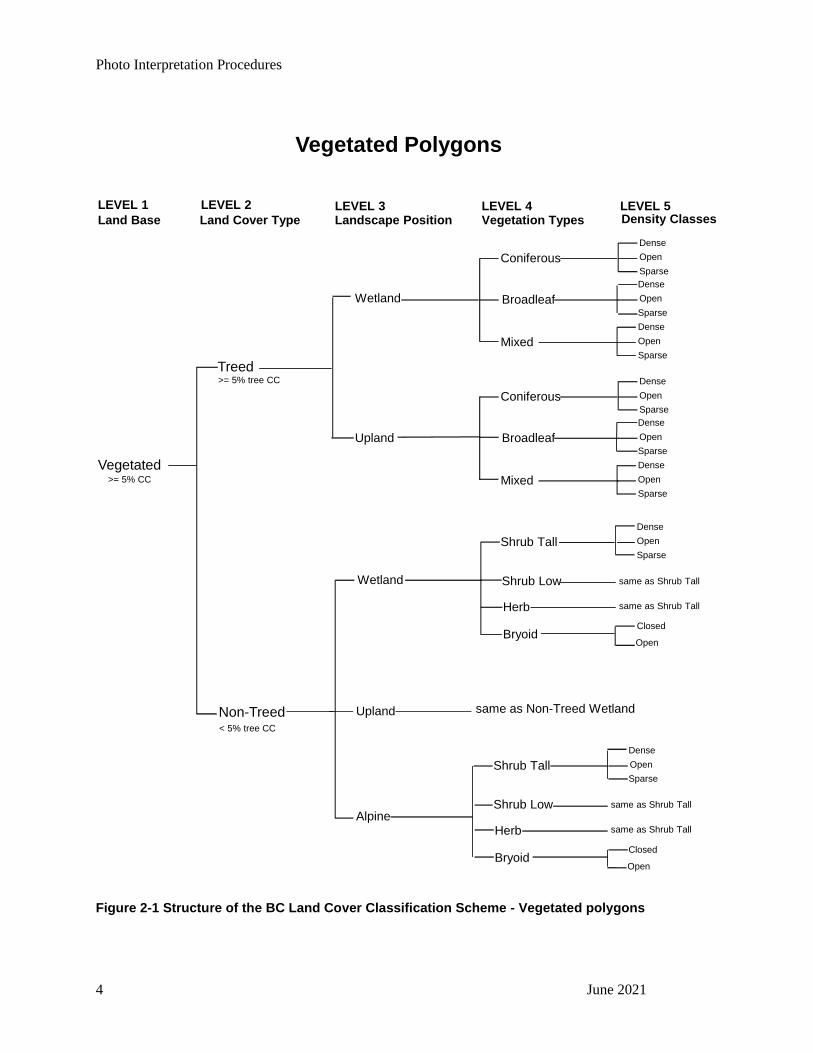
Photo Interpretation Procedures
4 June 2021
Figure 2-1 Structure of the BC Land Cover Classification Scheme - Vegetated polygons
Vegetated
Treed
Non-Treed
Wetland
Upland
Broadleaf
Mixed
LEVEL 1
Land Base
LEVEL 2
Land Cover TypeLEVEL 3Landscape Position
LEVEL 4Vegetation Types
LEVEL 5Density Classes
Vegetated Polygons
Coniferous Open
Sparse
Dense
Open
Sparse
Dense
Open
Sparse
Dense
Broadleaf
Mixed
Coniferous Open
Sparse
Dense
Open
Sparse
Dense
Open
Sparse
Dense
Shrub Tall
Shrub Low
Herb
Bryoid
Open
Sparse
Dense
same as Shrub Tall
same as Shrub Tall
Open
Closed
Wetland
Upland same as Non-Treed Wetland
Alpine
Shrub Tall
Shrub Low
Herb
Bryoid
Open
Sparse
Dense
same as Shrub Tall
same as Shrub Tall
Open
Closed
>= 5% tree CC
< 5% tree CC
>= 5% CC

Photo Interpretation Procedures
June 2021 5
Figure 2-2 Structure of the BC Land Cover Classification Scheme- Non-Vegetated polygons
Wetland
Upland
LEVEL 1
Land Base
LEVEL 2
Land Cover TypeLEVEL 3Landscape Position
LEVEL 4Non-Vegetated Cover Types
LEVEL 5Non-VegetatedCategories
Non-Vegetated Polygons
Non-Vegetated
Land
Alpine
Snow / Ice
Exposed Land
Detailed description
Detailed description
Rock / Rubble
Exposed Land
Detailed description
Detailed description
Snow / Ice
Detailed description
Wetland
Upland
Alpine
Detailed description
Detailed description
Detailed description
Water
Rock / Rubble Detailed description
Rock / Rubble
Exposed Land
Detailed description
Detailed description
Snow / Ice Detailed description
< 5% CC
Photo Interpretation Procedures
6 June 2021
The remainder of this section explains the land classification scheme in detail. For a discussion of the
derivation of land classification codes based on photo-interpreted estimates, see Section 13 Derived
Polygon Attributes.
2.2 Level 1 Land Base
2.2.1 Definition
The first level of the BC Land Cover Classification Scheme classifies the presence or absence of
vegetation within the boundaries of the polygon. Presence or absence is recognized by the vertical
projection of vegetation upon the land base within the polygon.
2.2.2 Purpose
Assessing the presence or absence of vegetation within the polygon provides the first level of
classification of the BC Land Cover Classification Scheme and the first level of reporting ability.
2.2.3 Procedure
V = Vegetated
A polygon is considered Vegetated when the total cover of trees, shrubs, herbs, and bryoids
(other than crustose lichens) covers at least 5% of the total surface area of the polygon.
N = Non-Vegetated
A polygon is considered Non-Vegetated when the total cover of trees, shrubs, herbs, and
bryoids (other than crustose lichens) covers less than 5% of the total surface area of the
polygon. Bodies of water are to be classified as Non-Vegetated.
U = Unreported
A polygon is classified as Unreported if it is within the mapsheet being reported on but is
outside the inventory unit of interest. The Unreported designation is restricted to areas where
inventory information is not currently available. Examples include National Parks, Provincial
Parks (where information is not available), Tree Farm Licenses and Tree Farms that are not in
the existing vegetation cover databases, and areas outside of the Province of British Columbia.
Note: Bodies of water may have vegetation on or under their surface; they are the responsibility of
others to evaluate.
2.3 Level 2 Land Cover Type
2.3.1 Definition
The second level of the BC Land Cover Classification Scheme classifies the polygon as to the land cover
type: treed or non-treed for vegetated polygons; land or water for non-vegetated polygons.
2.3.2 Purpose
Land cover type provides the second level of delineation within the BC Land Cover Classification
Scheme and provides the second level of reporting ability.
Photo Interpretation Procedures
June 2021 7
2.3.3 Procedure for Vegetated Polygons
An interpretation is made of the coverage of tree crowns as measured by their vertical projection upon the
land base, estimated to the nearest percentage crown closure.
T = Treed
A polygon is considered Treed if at least 5% of the polygon area, by live crown cover, consists
of tree species of any size.
N = Non-treed
A polygon is considered Non-Treed if less than 5% of the polygon area, by live crown cover,
consists of tree species of any size.
Note: The classification scheme applies to the entire land base, and equal care should be given to treed
and non-treed areas. Non-treed sites are an important part of the landscape as they often contain
many diverse and unique species and provide valuable habitats. Without a better appreciation for
the types of non-treed sites and their distribution, it will be more difficult to assemble new
information. Management interpretations and decisions at the large landscape level will be
enhanced with the addition of information on non-treed ecosystems.
2.3.4 Procedure for Non-Vegetated Polygons
The polygon is interpreted as the percentage area occupied by land or water. The cover type occupying
greater than 50% of the polygon area is the cover type to be assigned.
L = Land
The portion of the landscape not covered by water (as defined below), based on the percentage
area coverage.
W = Water
A naturally occurring, static body of water, or a watercourse formed when water flows between
continuous, definable banks. These flows may be intermittent or perennial but do not include
ephemeral flows where a channel with no definable banks is present. Islands within streams
that have definable banks are not part of the stream; gravel bars are part of the stream.
Interpretation is based on the percentage area coverage.
2.4 Level 3 Landscape Position for Vegetated and Non-Vegetated Polygons
2.4.1 Definition
The third level of the BC Land Cover Classification Scheme is the location of the polygon relative to
elevation and drainage and is described as either alpine, wetland, or upland. In rare cases, the polygon
may be an alpine wetland.
2.4.2 Purpose
The landscape position provides the framework for delineation of ecosystems and habitat and the third
level of reporting ability.
2.4.3 Procedure
The polygon is interpreted to see if it has one or more landscape positions. The polygon classification is
determined by the landscape position with the majority coverage by area.

Photo Interpretation Procedures
8 June 2021
W = Wetland
Land having the water table near, at, or above the soil surface, or which is saturated for a long
enough period to promote wetland or aquatic processes as indicated by poorly drained soils,
specialized vegetation, and various kinds of biological activity which are adapted to the wet
environment.
In the Canadian wetland classification, wetland classes include bogs, fens, marshes, swamps,
hot springs, hot pools, and shallow water. In British Columbia, Wetlands include forested or
non-forested sub-hydric (SMR 7) sites in addition to non-forested hydric (SMR 8) ecosystems
(see the BC Land Cover Classification document for a detailed description).
U = Upland
A broad class that includes all non-wetland ecosystems below Alpine that range from very
xeric, moss- and lichen-covered rock outcrops to highly productive forest ecosystems on hygric
(SMR 6) soils.
A = Alpine
Treeless by definition (for practical purposes, 1% tree cover or less can be included within the
alpine area) with vegetation dominated by shrubs, herbs, graminoids, bryoids, and lichens.
Much of the Alpine is non-vegetated, covered primarily by rock, ice, and snow.
The boundary between Alpine and Upland is drawn using the upper elevation of the discontinuous treed
area. The Alpine area will not typically include parkland and krummholz forest types. Generalization of
the boundary at a consistent elevation (varying with aspect) is necessary as cliffs, rock outcrops, and
avalanche chutes often dissect the Alpine/Upland transition. Alpine is a classification level of Non-Treed
areas above the tree line only.
Note: Alpine is the land area above the maximum elevation for tree species.
Parkland is a landscape characterized by strong clumping of trees due to environmental factors
(from Ecosystems of British Columbia, MoF, 1991).
Krummholz is the scrubby, stunted growth form of trees, often forming a characteristic zone at
the limit of tree growth at high elevations (from Forest Ecology Terms in Canada, Canadian
Forest Service, 1994).
2.5 Level 4 Vegetation Types and Non-Vegetated Cover Types
2.5.1 Definition
The fourth level of the BC Land Cover Classification Scheme classifies the vegetation types and Non-
Vegetated cover types (as described by the presence of distinct types upon the land base within the
polygon).
2.5.2 Purpose
Vegetation types and Non-Vegetated cover types provide the fourth level of delineation within the BC
Land Cover Classification Scheme and the fourth level of reporting ability.
2.5.3 Procedure for Vegetated Polygons
Vegetated polygons delineated and described in levels 1 to 3 in the land classification scheme are further
classified by the vegetation types as listed below. An interpretation is made of the coverage of vegetation

Photo Interpretation Procedures
June 2021 9
crown closure as measured by their vertical projection upon the land base, estimated to the nearest
percentage crown closure.
Treed Units
Treed units are split into three groups: Coniferous, Broadleaf, and Mixed.
TC = Treed - Coniferous
Defined as those trees found in BC within the order Coniferae. These trees are commonly
referred to as conifer or softwoods. The polygon is classified as Coniferous when the total basal
area (expressed as percentage species composition) of coniferous trees is 75% or more of the
total polygon tree basal area, and trees cover 5% or more of the total polygon area by crown
cover.
TB = Treed - Broadleaf
Defined as those trees classified botanically as Angiospermae in the subclass Dicotyledoneae.
These species are commonly referred to as deciduous or hardwoods. The polygon is classified
as Broadleaf when the total basal area (expressed as percentage species composition) of
broadleaf trees is 75% or more of the total polygon tree basal area, and trees cover a minimum
of 5% of the total polygon area by crown cover.
TM = Treed - Mixed
The polygon is classified as Mixed when neither coniferous nor broadleaf trees account for
75% or more of the total polygon tree basal area, and trees cover a minimum of 5% of the total
polygon area by crown cover.
Non-Treed Units
Non-Treed units are broken into Shrubs, Herbs, and Bryoids.
Shrubs are defined as multi-stemmed woody perennial plants, both evergreen and deciduous. A reporting
break is made between Tall (i.e. ≥ 2.0 m in height) and Low (i.e. < 2.0 m in height) for wildlife
management interpretation purposes. Other breaks may be reported by the user as height data are
estimated and stored as a continuous variable.
For a polygon to be classified as Non-Treed Shrub, it must have more than 5% total vegetation cover,
have less than 5% crown cover of trees, and have a minimum of 20% ground cover of shrubs, or shrubs
must constitute more than 1/3 of the total vegetation cover.
ST = Shrub Tall
A Shrub polygon with an average shrub height greater than or equal to 2.0 m. Shrub tall
includes species that are known to achieve heights of greater than 10 m but are specifically
excluded from the "tree" category in BC VRI Photo interpretation. These include willow (Salix
spp.) and alder species other than Red Alder (Alnus rubra).
SL = Shrub Low
A Shrub polygon with an average shrub height of less than 2.0 m.
Herbs are defined, for this system, as vascular plants without a woody stem, including ferns, fern allies,
some dwarf woody plants, grasses, and grass-like plants. The Herb class has two further subdivisions
based on the proportion of graminoids and forbs present:
Graminoids are defined as herbaceous plants with long, narrow leaves characterized by linear venation,
including grasses, sedges, rushes, and other related species.
Forbs are defined as herbaceous plants other than graminoids.
Photo Interpretation Procedures
10 June 2021
For a polygon to be classed as Non-Treed Herb it must have more than 5% total vegetation cover, have
less than 5% crown cover of trees, and have 20% or more ground cover of herbs, or herbs must constitute
more than 1/3 of the total vegetation cover, and the polygon must have less than 20% shrub cover.
HE = Herb
A Herb polygon with no distinction between forbs and graminoids.
HF = Herb - Forbs
A Herb polygon with forbs greater than 50% of the herb cover.
HG = Herb - Graminoids
A Herb polygon with graminoids greater than 50% of the herb cover.
Bryoids are defined as bryophytes (mosses, liverworts, and hornworts) and lichens (foliose or fruticose,
not crustose).
For a polygon to be classed as Non-Treed Bryoid, it must have more than 5% total vegetation cover, have
less than 5% crown cover of trees, and have greater than 50% of the vegetation cover in bryoids, and herb
and shrub cover must each be less than 20% crown cover.
BY = Bryoid
A Bryoid polygon with no distinction between mosses and lichens.
BM = Bryoid - Moss
A Bryoid polygon with mosses, liverworts, and hornworts greater than 50% of the bryoid
cover.
BL = Bryoid - Lichens
A Bryoid polygon with lichens (foliose or fruticose; not crustose) greater than 50% of the
bryoid cover.
2.5.4 Procedures for Non-Vegetated Polygons
Non-Vegetated polygons, delineated and described in levels 1 to 3 of the land classification scheme, are
further classified by the Non-Vegetated cover types listed below. An estimation is made of the class that
has the greatest percentage coverage by area.
Non-vegetated polygons (within the land cover type) are separated into three groups: Snow/Ice,
Rock/Rubble, and Exposed Land.
SI = Snow / Ice
Defined as either glacier, which is considered a mass of perennial snow and ice with definite
lateral limits, typically flowing in a particular direction, or other ice and snow cover that is not
part of a glacier.
RO = Rock / Rubble
Defined as bedrock or fragmented rock broken away from bedrock surfaces and moved into its
present position by gravity or ice. Extensive deposits are found in and adjacent to alpine areas
and are associated with steep rock walls and exposed ridges; canyons and cliff areas also
contain these deposits.
EL = Exposed Land
Contains all other forms of exposed land identified by a range of subclasses.
Note: The Water cover type (level 2) does not have any classes at this level of the land classification
scheme.
Photo Interpretation Procedures
June 2021 11
2.6 Level 5 Vegetated Density Classes and Non-Vegetated Categories
2.6.1 Definition
The fifth level of the BC Land Cover Classification Scheme classifies the vegetation density classes and
Non-Vegetated categories.
2.6.2 Purpose
Vegetated density classes and Non-Vegetated categories provide the fifth level of delineation within the
BC Land Cover Classification Scheme and the fifth level of reporting ability.
2.6.3 Procedure for Vegetated Polygons
The Vegetated polygons delineated and described in levels 1 to 4 in the land classification scheme are
further classified into density classes as listed below. Note that these are reporting breaks only, and
interpreters estimate density as a continuous variable.
The density classes for Treed, Shrub and Herb cover are as follows:
DE = Dense
Tree, shrub, or herb cover is between 61% and 100% for the polygon.
OP = Open
Tree, shrub, or herb cover is between 26% and 60% for the polygon.
SP = Sparse
Cover is between 5% and 25% for treed polygons, or cover is between 20% and 25% for shrub
or herb polygons.
The density classes for Bryoids are as follows:
CL = Closed
Cover of bryoids is greater than 50% of the polygon.
OP = Open
Cover of bryoids is less than or equal to 50% of the polygon.
2.6.4 Procedure for Non-Vegetated Polygons
Non-Vegetated polygons delineated and described in levels 1 to 3 in the land classification scheme are
further classified into categories as listed below.
Snow/Ice has two subclasses:
GL = Glacier
A mass of perennial snow and ice with definite lateral limits, typically flowing in a particular
direction.
PN = Snow Cover
Snow or ice that is not part of a glacier but is found during the summer months on the
landscape. (Care should be taken to determine if the snow on the imagery is a result of the photo
acquisition date. In such cases, the delineation or attribution procedure should be discussed with
the Ministry).
Rock/Rubble has five subclasses:
BR = Bedrock
Unfragmented, consolidated rock contiguous with the underlying material.

Photo Interpretation Procedures
12 June 2021
TA = Talus
Rock fragments of any size accumulated on or at the foot of slopes as a result of successive
rock falls. This is a type of colluvium.
BI = Blockfield
Blocks of rock derived from the underlying bedrock by weathering and/or frost heaving. These
have not undergone any significant down slope movement as they occur on level or gently
sloping areas.
MZ = Rubbly Mine Spoils
Discarded overburden or waste rock, moved to extract ore during mining.
LB = Lava Bed
An area where molten rock has flowed from a volcano or fissure and cooled and solidified to
form rock.
Exposed Land has nineteen subclasses:
RS = River Sediments
Silt, gravel, and sand bars associated with former river channels and present river edges.
ES = Exposed Soil
Any exposed soil not covered by the other categories, such as areas of recent disturbance that
include mud slides, debris torrents, avalanches, or disturbances such as pipeline rights-of-way
where vegetation cover is less than 5%. Exposed soil resulting from harvesting operations is
recognized in this category; however, harvested polygons must maintain a vegetated status.
LS = Pond or Lake Sediments
Exposed sediments related to dried lakes or ponds.
RM = Reservoir Margin
Land exposed by a drained or fluctuating reservoir. It is found above "normal" water levels and
may consist of a range of substrates, including gravel, cobbles, fine sediments, or bedrock.
BE = Beach
An area with sorted sediments reworked in recent time by wave action, which may be formed at
the edge of fresh or salt water bodies.
LL = Landing
A compacted area adjacent to a road used for sorting and loading logs.
BU = Burned Area
Land showing evidence of recent burning, either natural or prescribed. Vegetation with less
than 5% crown cover is present at the time of polygon description.
RZ = Road Surface
An area cleared and compacted for transporting goods and services by vehicles. Older roads
that are used infrequently or not at all may cease to be classed as Non-Vegetated.
MU = Mudflat
Flat plane-like areas that are associated with lakes, ponds, rivers, or streams and dominated by
fine-textured sediments. They can be associated with freshwater or estuarine sources.
CB = Cutbank
Part of a road corridor created upslope of the road surface, created by excavation into the
hillside.
MN = Moraine
An area of debris transported and deposited by a glacier.

Photo Interpretation Procedures
June 2021 13
GP = Gravel Pit
An area exposed through the removal of sand and gravel.
TZ = Tailings
An area containing the solid waste material produced in the mining and milling of ore.
RN = Railway Surface
A roadbed with fixed rails, which may contain single or multiple rail lines.
UR = Urban
Buildings and associated developments such as roads and parking areas which form an almost
continuous coverage of the landscape.
AP = Airport
A permanent, paved or gravel area, and associated buildings and parking used by airplanes.
MI = Open Pit Mine
An exposed area used to extract ore during a mining operation. This may contain associated
buildings and any tailing produced by the mining and milling process.
OT = Other
A Non-Vegetated polygon where none of the above categories can be reliably chosen.
DW = Downed wood
Consolidated coarse woody debris, blowdown, log decks, burn pile, or area of downed trees.
Water Cover (Level 2) has four subclasses:
LA = Lake
A naturally occurring static body of water. The boundary for the lake is the natural high-water
mark taken from Fresh Water Atlas if the feature is present. A dried-out lake bed should be
described as observed during photo interpretation and attributed according to the VRI standard.
RE = Reservoir
An artificial basin affected by impoundment behind a man-made structure such as a dam, berm,
dyke, or wall.
RI = River/Stream
A water course formed when water flows between continuous, definable banks. Flow may be
intermittent or perennial but does not include ephemeral flow where a channel with no definable
banks is present. Gravel bars are part of a stream, while islands within a stream that has
definable banks are not.
OC = Ocean
A naturally occurring body of water containing salt or generally considered to be salty.
Photo Interpretation Procedures
14 June 2021
3 Polygon Delineation
3.1 Introduction
Polygon delineation is based on the BC Land Cover Classification Scheme. This land classification
scheme includes both vegetated and non-vegetated cover classes over the entire provincial landscape.
Polygons identified by the land classification scheme are further divided into similar vegetated or non-
vegetated polygons. Detailed polygon attributes are assigned to each polygon, providing an estimated
base from which future Phase II Ground Sampling locations are selected.
3.1.1 Definition
Polygon delineation is the process used to divide the landscape into uniform polygons according to
defined criteria. Polygon delineation is based on observable differences in vegetated or non-vegetated
covers using aerial imagery.
3.1.2 Purpose
Delineating polygons provide boundaries for similar or "like" vegetated or non-vegetated land covers.
Accurate delineation provides logical units for the estimation of attributes.
3.1.3 Procedure
The photo interpreter normally proceeds from the general to the specific during the delineation process.
The order in which delineation is accomplished will vary from individual to individual, so the following
steps are provided as an example that may be modified as required. The photo interpreter will use the land
classification scheme to guide the process of delineating polygons. The primary types of attributes that
drive the delineation process are:
• Land classification scheme criteria
• Vegetation attributes
• Mensuration attribute
• Ecological attributes (where appropriate)
The objective of delineation is to identify distinctly recognizable vegetated or non-vegetated polygons
which are uniform or similar. In many cases, the polygon will be a complex of vegetated and/or non-
vegetated areas. In these cases, it may still be necessary to delineate the cover as one polygon due to the
limitations of minimum polygon size.
Example:
These steps may be taken to delineate a treed landscape on a mountain slope.
1. Delineate the alpine from the upland
2. Delineate areas of wetland
3. Delineate vegetated from non-vegetated
(A Vegetated polygon must have vegetation crown cover of 5% or greater.)
When the polygon is Vegetated, then:
Photo Interpretation Procedures
June 2021 15
1. Delineate Treed versus Non-Treed.
(A Treed polygon must have 5% or greater tree crown cover.)
Treed areas:
• Delineate Coniferous versus Broadleaf composition based on crown closure
• Further delineation will be done as appropriate for a combination of attributes such as species,
age, height, crown closure, or a combination of others
Non-Treed areas:
• Delineate by Shrub versus Herb versus Bryoid
• Further delineation will be done as appropriate for a combination of attributes such as shrub
height, herb cover type, vegetation density, and others
When a polygon is Non-Vegetated, then:
2. Delineate by category of Non-Vegetated cover type.
Guidelines
The delineation of polygons can be achieved with various differentiations that may be appropriate. In
order to achieve some consistency by each interpreter and between interpreters, the following guidelines
are suggested. These guidelines may vary depending on each user's needs and the complexity of the
project area. In many cases, information is available from silviculture on various stand conditions.
For normal aerial imagery, it is expected that delineation quality assurance will be performed at an
approximate ground scale of 1:5,000 in order to maintain consistency between interpreters and for Quality
Assurance purposes. This may be modified on a project-specific basis. In general:
• Polygon delineation must appear "smooth" and follow natural polygon boundaries and not have
sharp non-natural edges.
• All polygons must close.
• Polygon size must be consistent with the delineation guidelines set in the Photo Interpretation
Procedures.
• The interpreter should try to avoid significant areas where the delineation is within 40 m of other
delineation, with exceptions as noted elsewhere in the Photo Interpretation Procedures.
• General specifications for silviculture blocks are outlined in Section 13: RESULTS.
• Projects that are not using “puzzle” boundaries (see “Puzzle Boundaries” in section 3.1.3.4) for
project deliverables must be checked by the interpreter to ensure that polygons edge tie to
adjacent maps inside the project and outside the project as determined in the VPIP or contract
specifications.
• It is acceptable to use the project boundary as a polygon boundary.
• The interpreter is expected to review and correct any items identified in the random sample of
work evaluated by the quality assurance personnel, as requested by the Ministry.
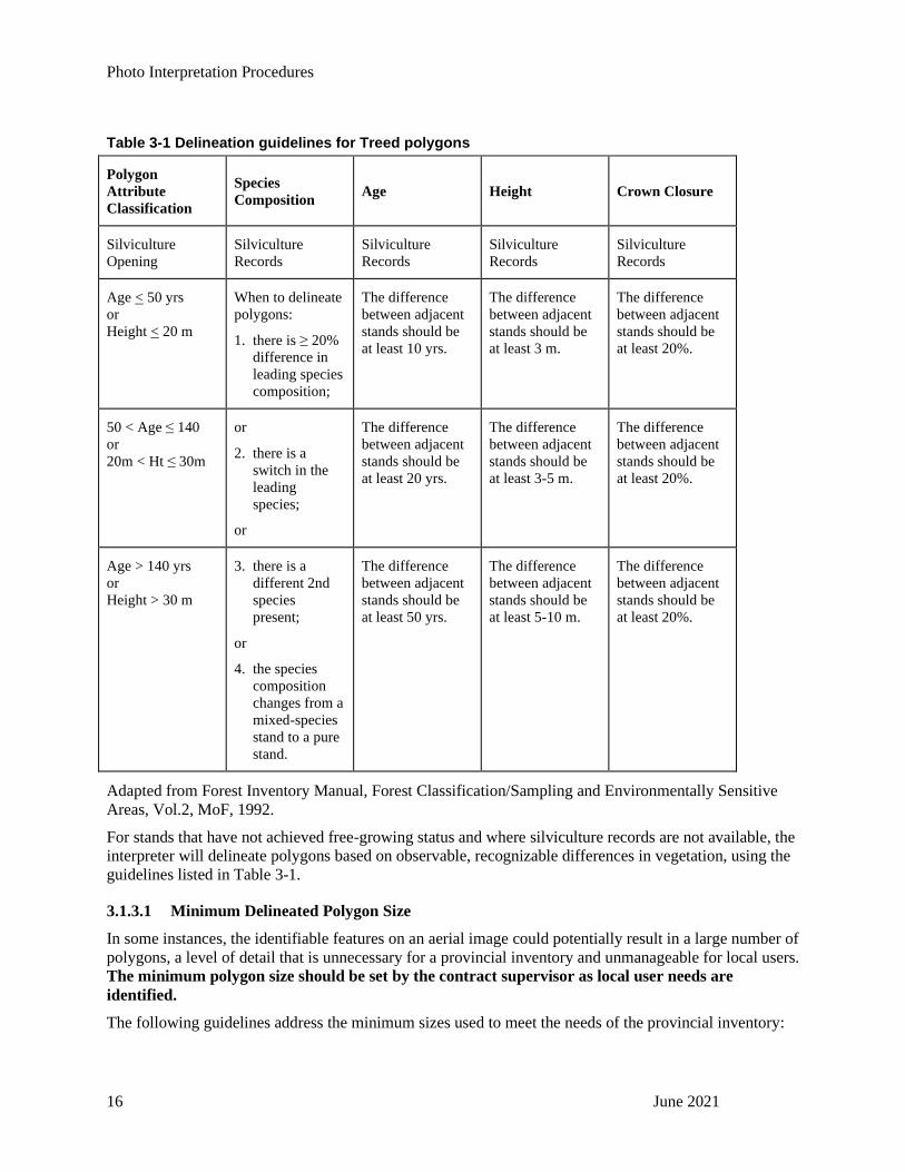
Photo Interpretation Procedures
16 June 2021
Table 3-1 Delineation guidelines for Treed polygons
Polygon
Attribute
Classification
Species
Composition Age Height Crown Closure
Silviculture
Opening
Silviculture
Records
Silviculture
Records
Silviculture
Records
Silviculture
Records
Age < 50 yrs
or
Height < 20 m
When to delineate
polygons:
1. there is ≥ 20%
difference in
leading species
composition;
The difference
between adjacent
stands should be
at least 10 yrs.
The difference
between adjacent
stands should be
at least 3 m.
The difference
between adjacent
stands should be
at least 20%.
50 < Age ≤ 140
or
20m < Ht ≤ 30m
or
2. there is a
switch in the
leading
species;
or
The difference
between adjacent
stands should be
at least 20 yrs.
The difference
between adjacent
stands should be
at least 3-5 m.
The difference
between adjacent
stands should be
at least 20%.
Age > 140 yrs
or
Height > 30 m
3. there is a
different 2nd
species
present;
or
4. the species
composition
changes from a
mixed-species
stand to a pure
stand.
The difference
between adjacent
stands should be
at least 50 yrs.
The difference
between adjacent
stands should be
at least 5-10 m.
The difference
between adjacent
stands should be
at least 20%.
Adapted from Forest Inventory Manual, Forest Classification/Sampling and Environmentally Sensitive
Areas, Vol.2, MoF, 1992.
For stands that have not achieved free-growing status and where silviculture records are not available, the
interpreter will delineate polygons based on observable, recognizable differences in vegetation, using the
guidelines listed in Table 3-1.
3.1.3.1 Minimum Delineated Polygon Size
In some instances, the identifiable features on an aerial image could potentially result in a large number of
polygons, a level of detail that is unnecessary for a provincial inventory and unmanageable for local users.
The minimum polygon size should be set by the contract supervisor as local user needs are
identified.
The following guidelines address the minimum sizes used to meet the needs of the provincial inventory:

Photo Interpretation Procedures
June 2021 17
Table 3-2 Summary of Minimum Delineated Polygon Guidelines
Polygon Type Minimum Size
Ministry-Provided Delineation
RESULTS Non-Free Growing Silviculture Openings
including reserve polygons within an opening
As Ministry-supplied in accordance with
Section 13.2.2
RESULTS Free Growing Silviculture Openings
including reserve polygons within an opening
> 2 ha minimum
Fresh Water Atlas polygon water features (i.e. lakes and
rivers)
> 0.5 ha minimum
Interpreter Delineated Polygons
Polygons with distinct attribute differences that create
obvious boundaries on the imagery (e.g. trees versus
shrub complex)
> 2 ha minimum
Polygons with indistinct attributes/boundaries as seen on
the imagery (e.g. tree heights change from 30 m to 25 m)
> 5 ha minimum
Polygons with an Alpine Designation of ‘A’
Delineate individual cover types ≥ 5 ha
into separate polygons where possible.
Otherwise, combine adjacent cover types <
5 ha into polygons with multiple land
cover components.
The minimum sizes to meet the needs of the provincial inventory are:
1. Areas with distinct boundaries - minimum 2 ha.
Where polygon boundaries are readily recognizable and distinct on the imagery, a minimum polygon size
of 2 hectares is appropriate.
For example: Treed versus Shrub complex; Herb complex versus Rock Talus area; abrupt change from 10
m trees to 32 m trees.
2. Areas with indistinct boundaries - minimum 5 ha.
Where polygon boundaries are not readily recognizable on the imagery, a minimum polygon size of 5
hectares is appropriate.
For example: a Treed area with a gradual height difference graduating from 30 m to 35 m; a repetitious
complex area with ridge and swale vegetation complexes; high-elevation Treed areas with dispersed
patches of rock outcrops.
3. Ministry-Supplied Water features
Modification to the imported Fresh Water Atlas (FWA) map features is generally not desired. Minor
defects are normally ignored, and delineation should be directly copied from the FWA. Major defects

Photo Interpretation Procedures
18 June 2021
discovered in the FWA dataset should be discussed with Ministry Inventory staff prior to re-delineation or
incorporation into the inventory. Revised waterbody delineation may also be submitted to GeoBC.
Areas where major inaccuracies occur typically include flat lands with meandering rivers or reservoirs.
The high-water marks (usually considered the vegetation line) along rivers and lake edges should be
captured due to seasonal water fluctuations. See examples below of FWA Lakes and FWA Rivers.
Figure 3-1 FWA Lake delineation needing modification
Figure 3-2 FWA River delineation needing modification

Photo Interpretation Procedures
June 2021 19
Figure 3-3 Reservoir lake boundary
3.1.3.2 Delineation of Dead Polygons
The remaining live trees normally drive polygon delineation in Treed polygons. However, additional
delineation is required when the estimated mortality exceeds a snag frequency of 100 stems/ha.
In polygons with dead trees and the combined crown closure of all live trees is ≥ 5% (i.e. the polygons is
Vegetated Treed (VTU or VTW)), use normal VRI delineation principles to establish boundaries between
polygons, and record the snag frequency for the polygon.
In polygons with dead trees and the combined crown closure of all trees is <5% (i.e. the polygon is now
Vegetated Non-Treed (VNU or VNW) and was Vegetated Treed (VTU or VTW)) prior to disturbance
(e.g. wildfire, mountain pine beetle (MPB) attack), delineate polygons based on BCLCCS Level 5 and
snag frequency.
For example, delineate an MPB-killed now classified as VNU, but previously VTU, to BCLCCS Level 5
(i.e. HE. BY, ST, SL), with further delineation based on the snag frequency.
3.1.3.3 Delineation of Linear Features
Avoid continuous areas where the delineation is parallel to and within 40 m of other delineation.
This rule is to be applied as a guideline, and smaller distances are acceptable in exceptional circumstances
to an absolute minimum distance of 15 m for non-Fresh Water Atlas, Digital Road Atlas or National
Railway Network features.
Linear features may sometimes require other exemptions to the minimum width criteria of 40 m between
polygons. As linear features may cross many mapsheets and interpreters, consistency is of importance
• All double line rivers are copied from the Fresh Water Atlas, and they will form polygons
regardless of width.
• Delineate roads, railways, and other man-made features only when the majority of the width of
the polygon to be created is greater than 40 m. The polygon will consist of the actual feature itself
and the associated right of way. The interpreter should review the entire length of the polygon
before delineating to make the determination. When a linear feature appears to become less than

Photo Interpretation Procedures
20 June 2021
40 m in width for greater than 2 km, then the interpreter should close off the polygon and include
the linear feature into the surrounding polygons.
Roads that travel through settlements (i.e. cities and towns) will not generally be delineated separately
from those features.
Figure 3-4 Example of unacceptable delineation of a linear feature – road right-of-way with continuous width under 40 m for more than 2 km.
When necessary, the use of the “bridging” technique is acceptable where the delineation is within 40 m of
other delineation to connect similar undersize types to a polygon with similar attributes.
Figure 3-5 Example of acceptable delineation within 40 m of other delineation

Photo Interpretation Procedures
June 2021 21
These are guidelines, but consistency must be maintained throughout a project and, where tied to other
projects, maintained between projects as much as possible.
Tips:
• Avoid detailed delineation in Non-Vegetated land.
• Avoid complicated, irregular type lines in landscapes with indistinct polygon boundaries. In areas
with distinct features, these irregular polygon boundaries may be valuable aids in navigation, etc.
• The following natural boundaries are polygons on the base map and therefore do not require
further delineation:
o double line rivers
o lake shores
o saltwater shores.
• Strive for consistency in delineation by each photo interpreter and between interpreters. Some
useful aids may be to:
o review daily project sample photos
o frequently discuss estimates, issues, and problems with other interpreters
o review the previous day’s photos before beginning the current day's activities.
3.1.3.4 Polygon Boundaries Along Project Area Edge and Between Internal Project Deliverables
Two methods may be employed to ensure continuity of delineation along the edge of a project or between
deliverables within a project. The methods to employ for a project will be determined in contract
specifications and may include a combination of the following techniques.
Puzzle Boundary Method
“Puzzle” boundaries are the preferred method of project and within deliverable polygon boundaries.
External project boundary
The project boundary has been set to follow the exact boundaries of the existing delineation of a previous
inventory project. The interpreter, therefore, will be responsible for delineation and attribution exactly up
to the boundary of the Project (vertices delineated must be identical to the project boundary).
Below is an example of a project boundary that matches the existing VRI delineation in an adjacent
project. The area to be interpreted in the Project is shown hatched in yellow, and a BCGS map boundary
is shown in red.
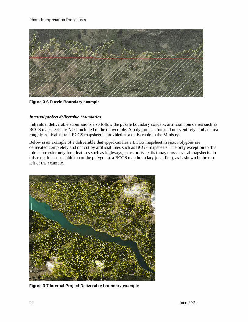
Photo Interpretation Procedures
22 June 2021
Figure 3-6 Puzzle Boundary example
Internal project deliverable boundaries
Individual deliverable submissions also follow the puzzle boundary concept; artificial boundaries such as
BCGS mapsheets are NOT included in the deliverable. A polygon is delineated in its entirety, and an area
roughly equivalent to a BCGS mapsheet is provided as a deliverable to the Ministry.
Below is an example of a deliverable that approximates a BCGS mapsheet in size. Polygons are
delineated completely and not cut by artificial lines such as BCGS mapsheets. The only exception to this
rule is for extremely long features such as highways, lakes or rivers that may cross several mapsheets. In
this case, it is acceptable to cut the polygon at a BCGS map boundary (neat line), as is shown in the top
left of the example.
Figure 3-7 Internal Project Deliverable boundary example

Photo Interpretation Procedures
June 2021 23
Final deliverables for surrounding mapsheets inside a project must match exactly (to the vertex) to
surrounding mapsheet deliverables as illustrated below.
Figure 3-8 Deliverable matching example
Edge Tie Method
The interpreter may be instructed to join delineated lines between currently ongoing projects or older
projects completed in previous years (edge ties). Typically, interpreters will only tie to inventories
completed to the current VRI standard, but decisions on whether to tie to adjacent projects will be
determined by the Ministry on a contract-specific basis.
When an interpreter is to edge tie delineation to another project, lines on both sides of the project must
join exactly (0 m tolerance), with a number of exceptions:
• The types stop at the project boundary – this may occur at cutblock edges that end at a TSA or
TFL boundary, where the line separating two adjacent polygons will stop at a cutblock boundary
that happens to be on the edge of the project.
• A boundary that follows along a project boundary within 20 m. When the polygon boundary
follows along the edge of the project, it is not necessary to create a separate polygon along the
boundary or offset the polygon boundary if it is within 20 m of the project boundary. The
interpreter does not need to jump back and forth between using a project boundary and using the
visual boundary if it varies inside and outside of 20 m along the polygon boundary. The intent is
to minimize very small sliver polygons along the edge of the project. The interpreter should send
screen captures to the project manager when in doubt.
• A significant change has occurred between the two projects. Examples include insect outbreaks or
wildfires that occurred after the adjacent inventory was completed and prior to the imagery being
taken in the current inventory.

Photo Interpretation Procedures
24 June 2021
• The delineation on the adjacent inventory is clearly incorrect. Minor differences will be tied to
exactly, but there may be cases where an obvious error was made in the adjacent inventory.
• New Silviculture opening information is available. The delineation will be updated to reflect new
RESULTS data even if it creates an edge tie mismatch.
Edge ties between individual submissions in a project should follow the same guidelines. Usually, the
edge of files delivered as a final product will follow mapsheet neatlines.
It is the interpreter’s responsibility to ensure that edge ties make sense as per the existing photos.

Photo Interpretation Procedures
June 2021 25
4 General Attributes
4.1 Introduction
Delineated polygons are assigned descriptions that are either estimates of polygon characteristics or
contain other information relating to the polygon. This section describes general attributes that include
information about the polygon and descriptions of ecological characteristics.
Polygons and the accompanying attributes may have applications in areas such as determining the
distribution and coverage of ecosystems, landscape patterns, wildlife habitat values, biological diversity,
land sensitivities for forestry, forest and ecosystem productivity, silviculture and harvesting options, and
land use planning. Government, private companies, and educational institutions will be major users of
such information.
Attributes are polygon-based estimates. The polygon is uniquely identified, and subsequent qualitative
and quantitative measurements are made for all Vegetated and Non-Vegetated covers observed in the
polygon. Cover types within the polygon, which are too small to delineate, may be described as land
cover components.
This section describes the process of identifying the polygon and estimating general attributes and
includes:
• Polygon number
• Surface expression
• Site position meso
• Soil nutrient regime
• Data source
• Modifying processes
• Alpine designation
4.2 Polygon Number
4.2.1 Definition
A polygon number is a unique number (i.e. Forest Cover Object ID) assigned to each Vegetated or Non-
Vegetated polygon after it is delineated. The intent is to assign a unique polygon number to each polygon
in British Columbia. As the polygon boundary or attributes change, a "new" unique number will be
assigned, and the "old" unique number will be archived.
4.2.2 Purpose
The polygon number provides the link between the graphic and descriptive files.
4.2.3 Procedure
Assign unique polygon numbers sequentially and systematically, based on a square-edged map,
throughout the project area (e.g. BCGS map sheet).
• Administrative boundaries do not constitute polygon boundaries.
• Forest Inventory Zones (FIZ) that separate coastal from interior forest zones do not constitute
polygon boundaries.
Figure 4.1 indicates one of the methods of polygon numbering for a BCGS map sheet.

Photo Interpretation Procedures
26 June 2021
Figure 4-1 One method of polygon numbering layout
4.3 Reference Year
4.3.1 Definition
The reference year is the year of the aerial imagery used in the inventory project.
4.3.2 Purpose
Reference year serves as a base for continually projecting and updating forest type attributes in the
database.
4.3.3 Interpretation Procedure
The year of the aerial imagery is entered for each polygon in the inventory project. The interpreter is
responsible for projecting previous data sources to the year of imagery for all inventory projects.
The Ministry uses Variable Density Yield Prediction (VDYP) software to “grow” or “project” the age,
height, volume and other attributes of polygons over time. The “reference year” for each polygon that
data is related to must be recorded appropriately for old data sources to enable the prediction software to
provide the correct projected attributes in current and future years.
Old data sources are a valuable source of information for interpreters, but not all of the data may be
present. For example, an old call may have age and height information but not basal area and density.
VDYP will only project data from one date, so all data that is provided must be related to the same year.
A polygon cannot have attributes that are correct for 1979 (e.g. an age and height), as well as attributes
that are correct in 2010 (basal area and density). The attributes below must ALL relate to the same year.
This year is recorded as the “Reference Year” regardless of the year of imagery.
• Age (leading and second species)
• Height (leading and second species)
• Basal Area
• Density
Poly gon # 1
Poly gon # 999
Poly gon # 500

Photo Interpretation Procedures
June 2021 27
When all of the above data is available for a data source, then the data will be entered in as-is from the
original data source, and the “Reference Year” will be the date of collection of the original data source.
As this data represents a single calibration point within the polygon, slight modifications to the attributes
are allowed to accommodate the polygon variability. VDYP will perform the “projection” of age, height,
etc., to the current and future years.
When any of the above items are not present in the old data source, portions of the data source attributes
are not going to be used by the interpreter, or large modifications are made to the data source attributes,
then the data source information must be revised (projected) by the interpreter so that all data is provided
relative to the date of imagery. The date of imagery will be used as the “Reference Year.” For example,
the interpreter must increase the age and height in the ground call to represent what is visible in the
imagery, which will now match the density and basal area that is visible in the photo.
Similarly, if a data source is NEWER than the year of imagery, all of the attributes must be referenced to
the same year. In most cases, a newer call will be to the VRI standard, so the reference year will be
recorded as the date of the calibration point (more recent) rather than the date of imagery (older).
4.4 Data Source Code
4.4.1 Definition
Data source refers to the primary source of information used for the attribute or attributes being described.
4.4.2 Purpose
The data source will provide an indication of the reliability of attribute descriptions. The data source may
also be used to assess training issues, such as the reliability of estimates with various data sources.
4.4.3 Procedures
Data sources provide calibration points to aid in the determination of polygon attributes. The interpreter
may (not) have data sources available within a polygon to aid in the interpretation. The interpreter will
use available data sources (Table 4-1) and interpretive skills to make appropriate attribute estimations.
The interpreter will:
• Assign one data source code to each of the following attributes or set of attributes:
o Ecological information (primarily SMR and SNR)
o Species composition
o Age of the leading species
o Height of the leading species
o Tree basal area
o Tree density
• When two or more data sources occur within the same polygon for a specific attribute or set of
attributes, use the attribute descriptions from the most appropriate source that describes the
polygon estimate.
• When several data sources are available, reference only the source used in the polygon attribute
estimate.
• In multi-layered stands, assign a data source code for each tree layer.
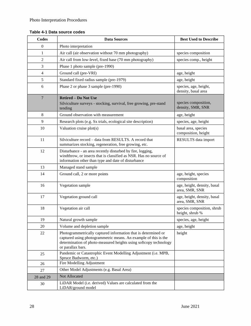
Photo Interpretation Procedures
28 June 2021
Table 4-1 Data source codes
Codes Data Sources Best Used to Describe
0 Photo interpretation
1 Air call (air observation without 70 mm photography) species composition
2 Air call from low-level, fixed base (70 mm photography) species comp., height
3 Phase 1 photo sample (pre-1990)
4 Ground call (pre-VRI) age, height
5 Standard fixed radius sample (pre-1979) age, height
6 Phase 2 or phase 3 sample (pre-1990) species, age, height,
density, basal area
7 Retired – Do Not Use
Silviculture surveys - stocking, survival, free growing, pre-stand
tending
species composition,
density, SMR, SNR
8 Ground observation with measurement age, height
9 Research plots (e.g. Sx trials, ecological site description) species, age, height
10 Valuation cruise plot(s) basal area, species
composition, height
11 Silviculture record – data from RESULTS. A record that
summarizes stocking, regeneration, free growing, etc.
RESULTS data import
12 Disturbance - an area recently disturbed by fire, logging,
windthrow, or insects that is classified as NSR. Has no source of
information other than type and date of disturbance
13 Managed stand sample
14 Ground call, 2 or more points age, height, species
composition
16 Vegetation sample age, height, density, basal
area, SMR, SNR
17 Vegetation ground call age, height, density, basal
area, SMR, SNR
18 Vegetation air call species composition, shrub
height, shrub %
19 Natural growth sample species, age, height
20 Volume and depletion sample age, height
22 Photogrammetrically captured information that is determined or
captured using photogrammetric means. An example of this is the
determination of photo-measured heights using softcopy technology
or parallax bars.
height
25 Pandemic or Catastrophic Event Modelling Adjustment (i.e. MPB,
Spruce Budworm, etc.)
26 Fire Modelling Adjustment
27 Other Model Adjustments (e.g. Basal Area)
28 and 29 Not Allocated
30 LiDAR Model (i.e. derived) Values are calculated from the
LiDAR/ground model

Photo Interpretation Procedures
June 2021 29
Codes Data Sources Best Used to Describe
31 LiDAR Canopy (calculated) Values are directly-measured from
LiDAR canopy data
32 to 39 Not Allocated
40 LVI derived values are calculated from the LVI models
41 LVI measured, values are from photo interpretation and/or
measured directly from a photo
42 to 49 Not Allocated
50 Medium Resolution interpreted satellite imagery (greater than 10 m
resolution)
51 High Resolution interpreted satellite imagery (less than 1o m
Resolution)
52 to 59 Not Allocated
60 Low Level, high res digital imagery interpreted (e.g. Digital
Camera System, DCS) values from high-resolution photo
interpretation
61 Low Level, high res digital imagery measured (i.e. Digital Camera
System, DCS) measured directly from high-resolution photography
4.4.4 Historical Data Sources
Historical Data Sources refer to data collected in previous inventory projects. These data sources could
include ground or air calls from previous VRI projects or older data collected to various standards in
place at the time of the project.
Interpreters must not use inventory classifications from the former forest cover inventory as a data source
unless data source points are not available. For example, a previous inventory polygon may have data
source code 4 (Ground Call 1 point). This label should NOT be used as a direct data source since the
previous interpreter may have modified the label for the polygon to account for differences between the
sample point and the rest of the polygon. New delineation will not match the historical polygon
boundaries, so the interpreted data from the previous inventory may not relate to the existing polygon.
The old interpretation could also be in error, and therefore ground or air measurements are preferable.
In Figure 4.2, a data source is shown in blue, old delineation from a previous inventory is shown in
yellow and new delineation from a current project is shown in red. The data source POINT is still usable
as a reference for red polygon A, but the polygon LABEL for the old forest cover as shown in yellow is
not appropriate as a direct label to use for polygons A or B, as the label reflects the old delineation which
covers portions of both new polygons.

Photo Interpretation Procedures
30 June 2021
Figure 4-2: Historical data source within old and new delineation
A data source code that represents the data source type (old ground or air call, etc.) will be recorded for
the polygon where the given attribute is used directly or is “grown” from the old data source and the old
data source falls within the polygon being interpreted. Extents of calls are not always available for old air
calls, and only a call centre point may be present. Air call labels should be used with caution when
applying to a new inventory. The call may have covered the entire polygon, and therefore may not
directly relate to the new delineation, similar to using the polygon label from the above example.
Not all data sources are of equal accuracy and reliability. Table 4-1 describes the relative reliability
associated with various data source types.
Table 4-2 Reliability of various VRI and pre-VRI data source types by attribute
Data Source
(Approximate Hierarchy of
Reliability)
Attribute Variation
Age Height Species
Composition
Even Multi-
Aged Even
Multi-
Height
Single
Species
Mixed
Species
VRI Data Sources
VRI Ground Call G G G G G G
VRI Air Call A A A A G G
Pre-VRI/ Historical Data Sources
Phase 2 or phase 3 samples (Pre-
VRI volume ground sampling)
G G G G G G
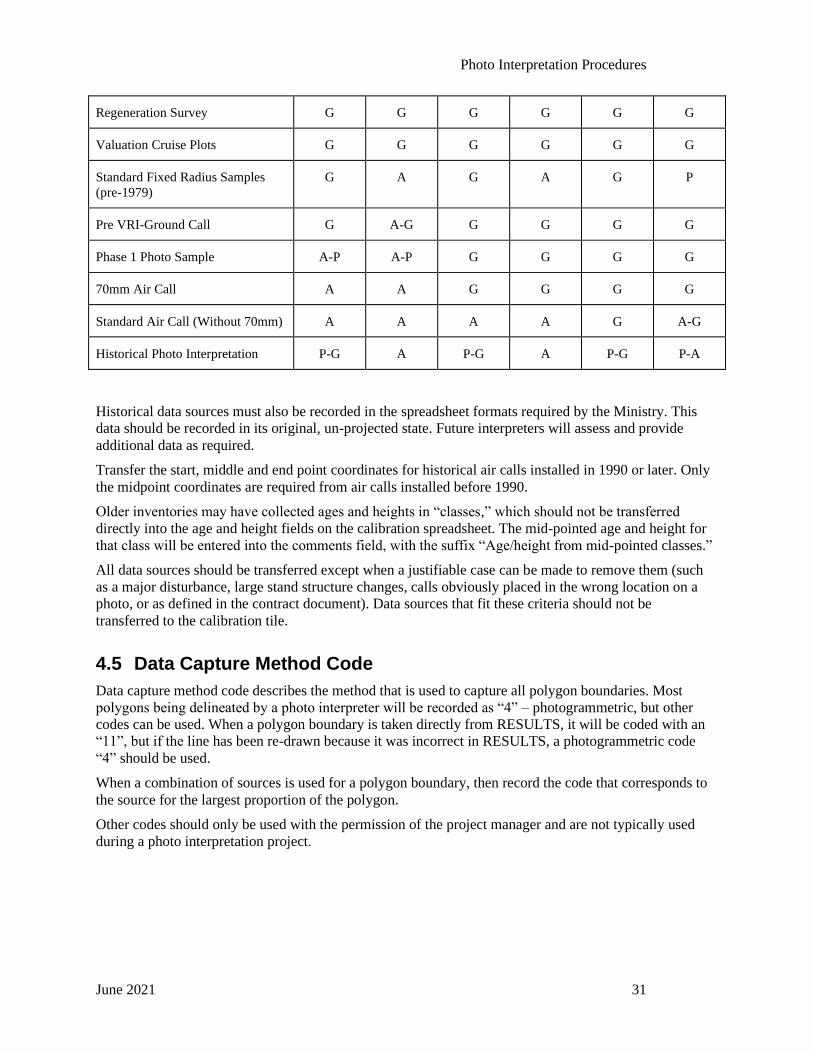
Photo Interpretation Procedures
June 2021 31
Regeneration Survey G G G G G G
Valuation Cruise Plots G G G G G G
Standard Fixed Radius Samples
(pre-1979)
G A G A G P
Pre VRI-Ground Call G A-G G G G G
Phase 1 Photo Sample A-P A-P G G G G
70mm Air Call A A G G G G
Standard Air Call (Without 70mm) A A A A G A-G
Historical Photo Interpretation P-G A P-G A P-G P-A
Historical data sources must also be recorded in the spreadsheet formats required by the Ministry. This
data should be recorded in its original, un-projected state. Future interpreters will assess and provide
additional data as required.
Transfer the start, middle and end point coordinates for historical air calls installed in 1990 or later. Only
the midpoint coordinates are required from air calls installed before 1990.
Older inventories may have collected ages and heights in “classes,” which should not be transferred
directly into the age and height fields on the calibration spreadsheet. The mid-pointed age and height for
that class will be entered into the comments field, with the suffix “Age/height from mid-pointed classes.”
All data sources should be transferred except when a justifiable case can be made to remove them (such
as a major disturbance, large stand structure changes, calls obviously placed in the wrong location on a
photo, or as defined in the contract document). Data sources that fit these criteria should not be
transferred to the calibration tile.
4.5 Data Capture Method Code
Data capture method code describes the method that is used to capture all polygon boundaries. Most
polygons being delineated by a photo interpreter will be recorded as “4” – photogrammetric, but other
codes can be used. When a polygon boundary is taken directly from RESULTS, it will be coded with an
“11”, but if the line has been re-drawn because it was incorrect in RESULTS, a photogrammetric code
“4” should be used.
When a combination of sources is used for a polygon boundary, then record the code that corresponds to
the source for the largest proportion of the polygon.
Other codes should only be used with the permission of the project manager and are not typically used
during a photo interpretation project.

Photo Interpretation Procedures
32 June 2021
Table 4-3 Data capture method codes
Codes Description Possible
Applications
4 Photogrammetric Most photo interpreted polygons and
imported water features lines from
(TRIM/FWA)
7 Digitizing Digitized directly from hard-copy
sources
8 Scanning
11 RESULTS Lines incorporated directly from
RESULTS
12 Other
14 Medium Resolution Satellite Imagery (> 10 m resolution)
15 Low-Resolution Satellite Imagery (< 10 m resolution)
16 LiDAR Imagery (Light Detection and Ranging)
4.6 Surface Expression
4.6.1 Definition
Surface expression refers to the form and patterns of form of the surficial material within the polygon. For
more detailed definitions and diagrams, refer to Terrain Classification System for British Columbia, D.
Howes and E. Kenk, MOE Manual 10, Version 2, 1997).
4.6.2 Purpose
Given the specialized nature of comprehensive terrain classification and the fact that the ground surface is
often blanketed by a canopy of trees, a simple classification attribute was selected. Surface expression is
relatively easy to photo interpret, and together with the attributes "modifying processes" and "site position
meso" will provide clues to soil parent material and useful site classification data.
4.6.3 Procedure
Assign the appropriate letter code (from Table 4-4) to each polygon. In polygons that have multiple
components, record the prevalent surface expression of the polygon on the basis of greatest percent area
coverage.
Table 4-4 Description of surface expression
Codes Description
C Cone
A cone, or segment of a cone, with a relatively smooth slope gradient greater than 15 degrees
(>25%).
D Depression
Circular or irregular area of lower elevation (such as a hollow) than the surrounding terrain;
depressions are greater than two metres deep. Examples are kettle holes and karst depressions
F Fan
A smooth segment of a cone with a slope gradient of up to 15 degrees (25%). Typically applied
to fluvial or alluvial fans.
Photo Interpretation Procedures
June 2021 33
Codes Description
H Hummock(s)
Steep-sided hillocks and hollows with slopes of 15 to 35 degrees (25 to 70%) predominant on
unconsolidated materials, and slopes of 15 to 90 degrees (25% to vertical) predominant on
bedrock. Slopes are non-linear (not parallel) but, generally, chaotic or dissected and rounded or
irregular in profile. Local relief is greater than one metre. Differentiated from undulating on the
basis of slope angle.
M Rolling
Elongated hillock(s) with slopes dominantly between 3 and 15 degrees (5 to 25%) with local
relief greater than one metre. Slopes are an assemblage of parallel or sub-parallel linear forms
with subdued relief and may occur in level or sloping meso slope positions.
N None of these descriptions apply as no apparent surface expression features are present.
P Plain
A level or gently sloping unidirectional surface with gradients of up to three degrees (5%). Local
surface irregularities generally have a relief of less than one metre. Commonly applied to
floodplains, organic deposits, lacustrine and marine plains, and the level portions of terraces and
deltas.
R Ridge(s)
Elongated or linear, parallel or sub-parallel hillock(s) or ridges with slopes predominantly
between 15 and 35 degrees (25 to 70%) on unconsolidated materials and between 15 and 90
degrees (25% to vertical) on bedrock. Local relief is greater than one metre. Differentiated from
rolling on the basis of slope angle. Possible locations include drumlinized till plains, eskers and
ridged bedrock. These may be created through the erosional effects of water.
T Terrace(s)
Step-like topography where each step-like form consists of both a scarp face and a horizontal or
gently inclined surface above it. The terrace description is applied to both the scarp and the flat
surface.
U Undulating
Gently sloping hillock(s) and hollow(s) with slopes of up to 15 degrees (25%). Local relief is
greater than one metre. Slopes are non-linear (not parallel), chaotic forms that are rounded or
irregular in profile.
4.7 Modifying Processes
4.7.1 Definition
Modifying processes are natural mechanisms of weathering, erosion and deposition that result in the
modification of surficial materials and land forms at the earth's surface (see p.39, Terrain Classification
System for British Columbia, D. Howes and E. Kenk, MOE Manual 10, Dec. 1988). Only active
modifying processes are to be assigned.
4.7.2 Purpose
Modifying processes are used for terrain classification. These processes provide information for site
classification, soil conditions, and identify potential hazards such as avalanches, slope instability, and
flooding.
Photo Interpretation Procedures
34 June 2021
4.7.3 Procedure
Assign the appropriate code (from Table 4-5) to each polygon. The code is recorded for the most
predominant modifying process within the polygon on the basis of percent area coverage. When a
modifying process is not observed in the polygon, “N” (None) should be entered in the column for this
attribute. A process is considered active if there is evidence of a current or recent occurrence or likely
future occurrence. This is not defined in quantitative terms (such as every 25 years) as the quantitative
assessment of frequency is often very difficult.
Table 4-5 Description of modifying processes
Codes Description
A Avalanching
Slopes modified by the rapid downslope movement of snow and ice and by the deposition of rock
debris, surficial material and vegetation debris transported by snow avalanches. Sites usually
contain avalanche chutes and run-out zones but may also be affected by ice falling from glaciers.
B River channelling
Erosion and channel formation by the flow of water within clearly defined banks.
F Mass movements
Down slope movement of cohesive or non-cohesive surficial material and/or bedrock by creeping,
sliding, flowing or falling. This includes rock and debris slides, soil slumps and talus slopes.
N None of these descriptions apply; no modifying processes are observed in the polygon.
U Flooding
Areas subject to periodic (possibly seasonal) inundation with subsequent deposition of soil
particles. Commonly applied to ephemeral lakes.
V Gully erosion
Modification of unconsolidated or consolidated surfaces by processes such as running water and
snow avalanching that result in the formation of parallel or sub-parallel long, narrow ravines.
Singular gullies are not generally included in this class.
4.8 Site Position Meso
4.8.1 Definition
Site position meso is the relative position of the polygon within a catchment area which often falls within
one of the major slope segments of site position macro. Site position macro applies to the scale
perspective from mountain top to main valley floor, with vertical distance in excess of 300 metres in most
mountain regions. The scale of vertical distance for site position meso is usually between 3 m and 300 m.
Ideally, site position meso applies to the scale of topography affecting surface water flow. In some simple
landscapes, site position meso and macro are the same (see p.31, Describing Ecosystems in the Field, H.
Luttmerding et al., MOE Manual 11, Dec. 1990).
4.8.2 Purpose
Site position meso is one of the key attributes for site series identification. Identification of soil moisture
regime, using environmental properties, is done with reference to categories of site position meso.
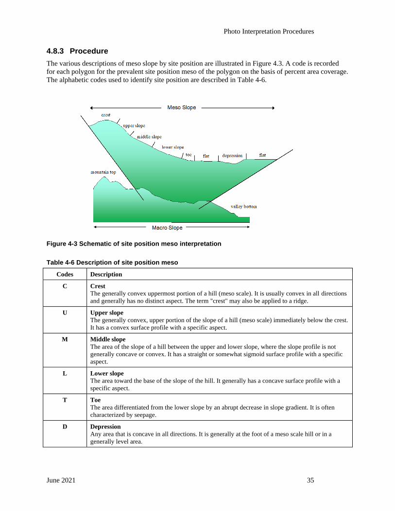
Photo Interpretation Procedures
June 2021 35
4.8.3 Procedure
The various descriptions of meso slope by site position are illustrated in Figure 4.3. A code is recorded
for each polygon for the prevalent site position meso of the polygon on the basis of percent area coverage.
The alphabetic codes used to identify site position are described in Table 4-6.
Figure 4-3 Schematic of site position meso interpretation
Table 4-6 Description of site position meso
Codes Description
C Crest
The generally convex uppermost portion of a hill (meso scale). It is usually convex in all directions
and generally has no distinct aspect. The term "crest" may also be applied to a ridge.
U Upper slope
The generally convex, upper portion of the slope of a hill (meso scale) immediately below the crest.
It has a convex surface profile with a specific aspect.
M Middle slope
The area of the slope of a hill between the upper and lower slope, where the slope profile is not
generally concave or convex. It has a straight or somewhat sigmoid surface profile with a specific
aspect.
L Lower slope
The area toward the base of the slope of the hill. It generally has a concave surface profile with a
specific aspect.
T Toe
The area differentiated from the lower slope by an abrupt decrease in slope gradient. It is often
characterized by seepage.
D Depression
Any area that is concave in all directions. It is generally at the foot of a meso scale hill or in a
generally level area.
Photo Interpretation Procedures
36 June 2021
Codes Description
F Flat (Level)
Any level area not immediately adjacent to a meso scale hill (or toe). The surface profile is
generally horizontal with no significant aspect.
4.9 Alpine Designation
4.9.1 Definition
Alpine designation pertains to one category of landscape position (the third level of the BC Land Cover
Classification Scheme). It describes the location of the polygon relative to elevation by assigning a
classification: Alpine or Not Alpine. Subsequent information on the relative soil moisture regime (SMR)
will identify Wetlands.
4.9.2 Purpose
Alpine designation contributes to the framework for delineation of ecosystems and habitat and the third
level of reporting ability.
4.9.3 Procedure
The polygon is interpreted to see if it is above or below the tree line. The boundary between Upland and
Alpine is drawn using the upper elevation of the discontinuous treed area. The alpine areas will not
typically include parkland and krummholz forest types.
Note: Alpine is the land area above the maximum elevation for trees.
Parkland is a landscape characterized by strong clumping of trees due to environmental factors
(from Ecosystems of British Columbia, MoF, 1991).
Krummholz is the scrubby, stunted growth form of trees, often forming a characteristic zone at
the limit of tree growth at high elevations (from Forest Ecology Terms in Canada, Canadian
Forest Service, 1994).
Generalization of the Alpine boundary at a consistent elevation (varying with aspect) is necessary as
cliffs, rock outcrops, and avalanche chutes often dissect the Alpine/Upland transition.
Assign the appropriate code to each polygon (see Table 4-7).
Table 4-7 Description of alpine designation
Codes Description
A Alpine
Alpine is the land area above the maximum elevation for tree species, dominated in vegetated
areas by shrubs, herbs, bryoids and lichens. Much of the Alpine is non-vegetated, covered
primarily by rock, ice and snow. The Alpine is treeless by definition; however, there may be a
few rare trees (<1% crown closure).
N Not Alpine
Areas not included in Alpine areas, as defined above.
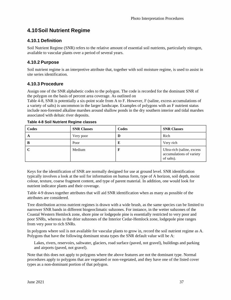
Photo Interpretation Procedures
June 2021 37
4.10 Soil Nutrient Regime
4.10.1 Definition
Soil Nutrient Regime (SNR) refers to the relative amount of essential soil nutrients, particularly nitrogen,
available to vascular plants over a period of several years.
4.10.2 Purpose
Soil nutrient regime is an interpretive attribute that, together with soil moisture regime, is used to assist in
site series identification.
4.10.3 Procedure
Assign one of the SNR alphabetic codes to the polygon. The code is recorded for the dominant SNR of
the polygon on the basis of percent area coverage. As outlined on
Table 4-8, SNR is potentially a six-point scale from A to F. However, F (saline, excess accumulations of
a variety of salts) is uncommon in the larger landscape. Examples of polygons with an F nutrient status
include non-forested alkaline marshes around shallow ponds in the dry southern interior and tidal marshes
associated with deltaic river deposits.
Table 4-8 Soil Nutrient Regime classes
Codes SNR Classes Codes SNR Classes
A Very poor D Rich
B Poor E Very rich
C Medium F Ultra-rich (saline, excess
accumulations of variety
of salts).
Keys for the identification of SNR are normally designed for use at ground level. SNR identification
typically involves a look at the soil for information on humus form, type of A horizon, soil depth, moist
colour, texture, coarse fragment content, and type of parent material. In addition, one would look for
nutrient indicator plants and their coverage.
Table 4-9 draws together attributes that will aid SNR identification when as many as possible of the
attributes are considered.
Tree distribution across nutrient regimes is drawn with a wide brush, as the same species can be limited to
narrower SNR bands in different biogeoclimatic subzones. For instance, in the wetter subzones of the
Coastal Western Hemlock zone, shore pine or lodgepole pine is essentially restricted to very poor and
poor SNRs, whereas in the drier subzones of the Interior Cedar-Hemlock zone, lodgepole pine ranges
from very poor to rich SNRs.
In polygons where soil is not available for vascular plants to grow in, record the soil nutrient regime as A.
Polygons that have the following dominant strata types the SNR default value will be A:
Lakes, rivers, reservoirs, saltwater, glaciers, road surface (paved, not gravel), buildings and parking
and airports (paved, not gravel).
Note that this does not apply to polygons where the above features are not the dominant type. Normal
procedures apply to polygons that are vegetated or non-vegetated, and they have one of the listed cover
types as a non-dominant portion of that polygon.

Photo Interpretation Procedures
38 June 2021
For water bodies, note that the standard code for the ecology features is:
Surface expression = D (depression)
Modifying processes = N (none)
Site position meso = D (depression)
Alpine designation = A or N, dependent on landscape location
Soil nutrient regime = A (very poor)
Table 4-9 A selection of attributes to assist estimation of SNR through photo interpretation
Generalized SNR Poor Medium Rich
Soil
Nutrient
Regime
A B
very poor
poor
C
medium
D E
rich very
rich
Site Position Meso upper middle lower
Mineral Soil Matrix coarse medium fine
Cover Of Rock Outcrops high (>50%) medium (15-50%) low (<15%)
Rock Type
conglomerate
quartzite
sandstone
other rock types
dolomite
limestone
Relative Productivity Low Medium High
Proposed SNR Relations For Selected Tree Species In Their Main Climatic Distributional Range:
Douglas-fir <------------------------------------------Fd---------------------------------------->
Yellow-cedar <------------------------------------------Yc---------------------------------------->
Western red cedar <------------------------------------------Cw---------------------------------------->
Black spruce <----------------------Sb-------------------->
Shore and lodgepole pine <----------------------Pl-------------------------------->
Arbutus <-------------------Ra-------------->
Western hemlock <-------------------------Hw------------------->
Mountain hemlock <-------------------------Hm------------------->
Trembling aspen <-------------------------------------------At-------------------------------->
Paper birch <--------------------------Ep--------------------------->
Red alder <--------------------------Dr------------------------------------>
Engelmann spruce <---------------------Se-------------------------->
White spruce <---------------------Sw------------------------->
Whitebark pine <-----------------Pa------------------------->
Western larch <-----------------Lw------------------------>
Alpine larch <--------------------------La--------------------------->
Grand fir <-------------------Bg------------->
Amabilis fir <-------------------Ba------------->
Subalpine fir <-------------------Bl------------->
Yellow (ponderosa) pine <--------------------------Py------------------------>
Garry oak <--------------------------Qg----------------------->
Sitka spruce <-----------------------Ss------------------->
Bigleaf maple <---------------Mb------------------->
Tamarack <----------------Lt-------------------->
Balsam poplar <---------Acb------------------>
Black cottonwood <---Act------------------->
Note: These are only guidelines and not intended to substitute regular field truth checks and practical knowledge of
site classification as presented in the Ministry of Forests “Field Guide for Site Identification and Interpretation ...”
for the forest region in question. The tree nutritional relations interpretations have been adapted from Karjina, V.J.,
K. Klinka and J. Worrall. 1982. Distribution and ecological characteristics of trees and shrubs of British Columbia.
UBC Faculty of Forestry. 131 pp. T. Lewis has provided valuable suggestions and ideas for this key.

Photo Interpretation Procedures
June 2021 39
5 Land Cover Component Attributes
5.1 Introduction
Land cover types within the polygon that contribute to the overall polygon description but are too small
to be delineated using current guidelines may be described by land cover components. The intent is to
determine the ecological function of the polygon. For each land cover component identified within a
polygon, percent area coverage and a soil moisture regime will be recorded. For information on deriving
land cover class and soil moisture regime at the polygon level, refer to Section 13 Derived Attributes.
The process of determining Land Cover Components is independent of the derived BC Land Cover
Classification Scheme. For example, 8% vegetated cover on a talus slope; the Land Cover Component for
this polygon would still be TA100.
5.2 Land Cover Components (LCC #1, #2, #3)
5.2.1 Definition
Land cover component identifies the ecological function of the polygon or portions of the polygon.
5.2.2 Purpose
The land cover component identifies the entire polygon or a portion of the total polygon area that would
be uniquely described if finer delineation criteria were applied. This information will provide a further
spatial description of each land cover component for forest management purposes and will also be used in
the interpretation of wildlife habitat.
5.2.3 Procedure
Enter the appropriate two-letter code (see Table 5-1) for any polygon component that:
• Consists of continuous area(s) that are individually greater than or equal to 10% of the polygon
area
• Would otherwise be delineated and classified at approximately twice the map scale.
Describe up to three land cover components (in decreasing size, by area).
Enter the appropriate code under Land Cover Component #1, Land Cover Component #2 and Land Cover
Component #3.
When more than three components exist, the remaining percent cover is recorded under "Other Land
Cover Component Percent Coverage."

Photo Interpretation Procedures
40 June 2021
Table 5-1 Land cover component codes
Codes Description
TB Treed Broadleaf
A Treed polygon where 75% or more of the live tree basal area, expressed as percentage species
composition, consists of broadleaf cover.
TC Treed Coniferous
A Treed polygon where 75% or more of the live tree basal area, expressed as percentage species
composition, consists of coniferous cover.
TM Treed Mixed
A Treed polygon where neither coniferous nor broadleaf cover individually constitutes at least 75%
of the live tree basal area, expressed as percentage species composition.
ST Shrub Tall
A Shrub polygon with shrub height of two metres or more.
SL Shrub Low
A Shrub polygon with shrub height less than two metres.
HE Herb
A Herb polygon with no distinction between forbs and graminoids.
HF Herb - Forbs
A Herb polygon with forbs greater than 50% of the herb cover.
HG Herb - Graminoids
A Herb polygon with graminoids greater than 50% of the herb cover.
BY Bryoid
A Bryoid polygon with no distinction between mosses and lichens.
BM Bryoid - Moss (bryophytes)
A Bryoid polygon with bryophytes greater than 50% of the bryoid cover.
BL Bryoid - Lichens
A Bryoid polygon with lichens greater than 50% of the bryoid cover.
SI Snow / Ice
Either glacier (which is considered a mass of perennial snow and ice with definite lateral limits,
typically flowing in a particular direction) or other ice and snow cover that is not part of a glacier.
GL Glacier
A mass of perennial snow and ice with definite lateral limits, typically flowing in a particular
direction.
PN Snow Cover
Snow or ice that is not part of a glacier but is found during the summer months on the landscape.
(Care should be taken to determine if the snow on the imagery is a result of the photo acquisition
date. In such cases, the delineation or attribution procedure should be discussed with the Ministry).
RO Rock / Rubble
Bedrock or fragmented rock broken away from bedrock surfaces and moved into its present position
by gravity or ice. Extensive deposits are found in and adjacent to alpine areas and are associated with
steep rock walls and exposed ridges; canyons and cliff areas also contain these deposits.
BR Bedrock
Unfragmented, consolidated rock contiguous with underlying material.
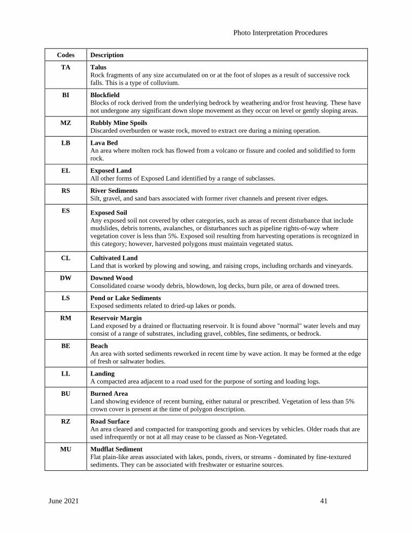
Photo Interpretation Procedures
June 2021 41
Codes Description
TA Talus
Rock fragments of any size accumulated on or at the foot of slopes as a result of successive rock
falls. This is a type of colluvium.
BI Blockfield
Blocks of rock derived from the underlying bedrock by weathering and/or frost heaving. These have
not undergone any significant down slope movement as they occur on level or gently sloping areas.
MZ Rubbly Mine Spoils
Discarded overburden or waste rock, moved to extract ore during a mining operation.
LB Lava Bed
An area where molten rock has flowed from a volcano or fissure and cooled and solidified to form
rock.
EL Exposed Land
All other forms of Exposed Land identified by a range of subclasses.
RS River Sediments
Silt, gravel, and sand bars associated with former river channels and present river edges.
ES Exposed Soil
Any exposed soil not covered by other categories, such as areas of recent disturbance that include
mudslides, debris torrents, avalanches, or disturbances such as pipeline rights-of-way where
vegetation cover is less than 5%. Exposed soil resulting from harvesting operations is recognized in
this category; however, harvested polygons must maintain vegetated status.
CL Cultivated Land
Land that is worked by plowing and sowing, and raising crops, including orchards and vineyards.
DW Downed Wood
Consolidated coarse woody debris, blowdown, log decks, burn pile, or area of downed trees.
LS Pond or Lake Sediments
Exposed sediments related to dried-up lakes or ponds.
RM Reservoir Margin
Land exposed by a drained or fluctuating reservoir. It is found above "normal" water levels and may
consist of a range of substrates, including gravel, cobbles, fine sediments, or bedrock.
BE Beach
An area with sorted sediments reworked in recent time by wave action. It may be formed at the edge
of fresh or saltwater bodies.
LL Landing
A compacted area adjacent to a road used for the purpose of sorting and loading logs.
BU Burned Area
Land showing evidence of recent burning, either natural or prescribed. Vegetation of less than 5%
crown cover is present at the time of polygon description.
RZ Road Surface
An area cleared and compacted for transporting goods and services by vehicles. Older roads that are
used infrequently or not at all may cease to be classed as Non-Vegetated.
MU Mudflat Sediment
Flat plain-like areas associated with lakes, ponds, rivers, or streams - dominated by fine-textured
sediments. They can be associated with freshwater or estuarine sources.
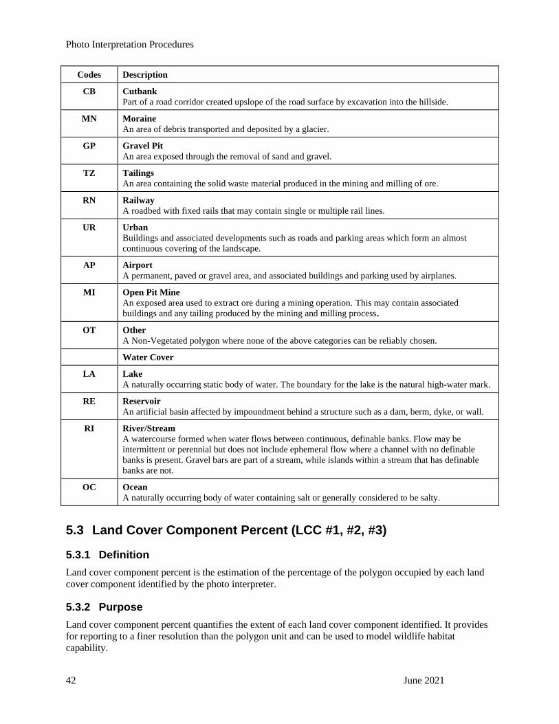
Photo Interpretation Procedures
42 June 2021
Codes Description
CB Cutbank
Part of a road corridor created upslope of the road surface by excavation into the hillside.
MN Moraine
An area of debris transported and deposited by a glacier.
GP Gravel Pit
An area exposed through the removal of sand and gravel.
TZ Tailings
An area containing the solid waste material produced in the mining and milling of ore.
RN Railway
A roadbed with fixed rails that may contain single or multiple rail lines.
UR Urban
Buildings and associated developments such as roads and parking areas which form an almost
continuous covering of the landscape.
AP Airport
A permanent, paved or gravel area, and associated buildings and parking used by airplanes.
MI Open Pit Mine
An exposed area used to extract ore during a mining operation. This may contain associated
buildings and any tailing produced by the mining and milling process.
OT Other
A Non-Vegetated polygon where none of the above categories can be reliably chosen.
Water Cover
LA Lake
A naturally occurring static body of water. The boundary for the lake is the natural high-water mark.
RE Reservoir
An artificial basin affected by impoundment behind a structure such as a dam, berm, dyke, or wall.
RI River/Stream
A watercourse formed when water flows between continuous, definable banks. Flow may be
intermittent or perennial but does not include ephemeral flow where a channel with no definable
banks is present. Gravel bars are part of a stream, while islands within a stream that has definable
banks are not.
OC Ocean
A naturally occurring body of water containing salt or generally considered to be salty.
5.3 Land Cover Component Percent (LCC #1, #2, #3)
5.3.1 Definition
Land cover component percent is the estimation of the percentage of the polygon occupied by each land
cover component identified by the photo interpreter.
5.3.2 Purpose
Land cover component percent quantifies the extent of each land cover component identified. It provides
for reporting to a finer resolution than the polygon unit and can be used to model wildlife habitat
capability.
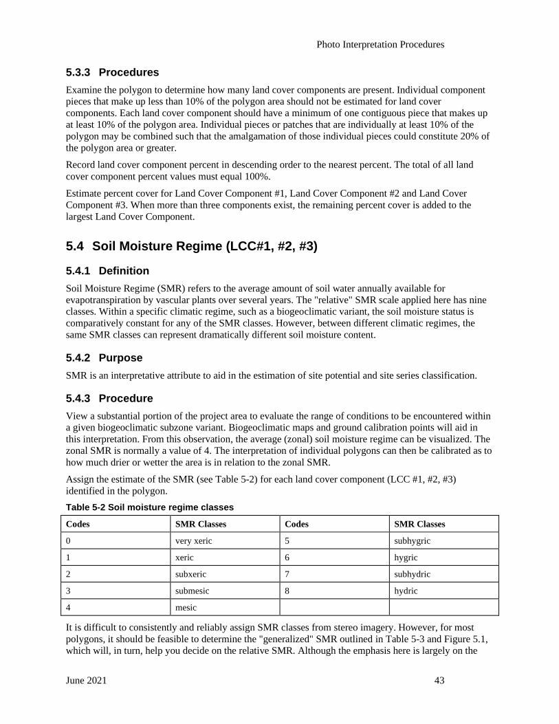
Photo Interpretation Procedures
June 2021 43
5.3.3 Procedures
Examine the polygon to determine how many land cover components are present. Individual component
pieces that make up less than 10% of the polygon area should not be estimated for land cover
components. Each land cover component should have a minimum of one contiguous piece that makes up
at least 10% of the polygon area. Individual pieces or patches that are individually at least 10% of the
polygon may be combined such that the amalgamation of those individual pieces could constitute 20% of
the polygon area or greater.
Record land cover component percent in descending order to the nearest percent. The total of all land
cover component percent values must equal 100%.
Estimate percent cover for Land Cover Component #1, Land Cover Component #2 and Land Cover
Component #3. When more than three components exist, the remaining percent cover is added to the
largest Land Cover Component.
5.4 Soil Moisture Regime (LCC#1, #2, #3)
5.4.1 Definition
Soil Moisture Regime (SMR) refers to the average amount of soil water annually available for
evapotranspiration by vascular plants over several years. The "relative" SMR scale applied here has nine
classes. Within a specific climatic regime, such as a biogeoclimatic variant, the soil moisture status is
comparatively constant for any of the SMR classes. However, between different climatic regimes, the
same SMR classes can represent dramatically different soil moisture content.
5.4.2 Purpose
SMR is an interpretative attribute to aid in the estimation of site potential and site series classification.
5.4.3 Procedure
View a substantial portion of the project area to evaluate the range of conditions to be encountered within
a given biogeoclimatic subzone variant. Biogeoclimatic maps and ground calibration points will aid in
this interpretation. From this observation, the average (zonal) soil moisture regime can be visualized. The
zonal SMR is normally a value of 4. The interpretation of individual polygons can then be calibrated as to
how much drier or wetter the area is in relation to the zonal SMR.
Assign the estimate of the SMR (see Table 5-2) for each land cover component (LCC #1, #2, #3)
identified in the polygon.
Table 5-2 Soil moisture regime classes
Codes SMR Classes Codes SMR Classes
0 very xeric 5 subhygric
1 xeric 6 hygric
2 subxeric 7 subhydric
3 submesic 8 hydric
4 mesic
It is difficult to consistently and reliably assign SMR classes from stereo imagery. However, for most
polygons, it should be feasible to determine the "generalized" SMR outlined in Table 5-3 and Figure 5.1,
which will, in turn, help you decide on the relative SMR. Although the emphasis here is largely on the

Photo Interpretation Procedures
44 June 2021
physical features of the landscape, vegetation species composition and vigour obviously play an important
role in the SMR decision. Furthermore, the Ministry of Forests' biogeoclimatic subzone and variant maps
for the different forest regions in the province, in combination with the accompanying field guides for site
identification, will provide practical reference information.
For land cover components where soil is not available for vascular plants to establish and grow in, the soil
moisture regime field should be recorded as zero (0).
As each land cover component is given a unique SMR value, it is possible that a particular polygon may
have both an LCC with an SMR value and an LCC without an SMR value.
The following cover types should have a zero (0) attribute in the SMR field:
Road surface, buildings, parking and airports.
Soil moisture attribute should be recorded as a blank for lakes, rivers, reservoirs, saltwater and glaciers.
Guidelines
The following guidelines can be used to aid estimation of SMR:
• SMR can be inferred from selected physiographic and soil features
• SMR classes, particularly 0 to 5, do not reflect the actual amount of available water as this is a
function of climate
• SMR is based on annual water balance and water table depth
• Very dry and dry classes represent growing season water deficits
• Circum-mesic classes represent regimes with neither deficits nor surpluses during the growing
season
• Seepage, wet, and aqueous classes indicate growing season water surpluses, often with shallow
water tables
• Wet and aqueous classes are, by definition, "wetlands"
• SMR can be indirectly inferred using indicator plants
Table 5-3 and Figure 5.1 will assist in the photo interpretation of SMR. Table 5-3 indicates the
relationship between SMR and soil nutrient regime (SNR). It also provides assistance to the photo
interpreter in determining generalized SMR.

Photo Interpretation Procedures
June 2021 45
Table 5-3 Relative and generalized SMR and SNR Guide
GENERALIZED SOIL NUTRIENT REGIME
P M R GENERALIZED
SOIL PRIMARY poor medium rich SOIL
MOISTURE WATER RELATIVE SOIL NUTRIENT REGIME MOISTURE
REGIME SOURCE A
very
poor
B
poor
C
medium
D
rich
E
very
rich
F
ultra-
rich,
saline
REGIME
VERY
XERIC
0
precipitation VERY DRY
(V)
XERIC
1
precipitation
SUBXERIC
2
precipitation DRY
(D)
SUBMESIC
3
precipitation
MESIC
4
precipitation
in moderately
fine-textured
soils & limited
seepage in
coarse-textured
soils
CIRCUM-MESIC
(CM)
SUBHYGRIC
5
precipitation
and seepage
HYGRIC
6
seepage SEEPAGE
(S)
SUBHYDRIC
7
seepage of
permanent
water table
WET
(WT)
HYDRIC
8
permanent
water table
AQUEOUS
(AQ)
Adapted from A Field Guide for Site Identification and
Interpretation for the Vancouver Forest Region, LMH 28, 1994

Photo Interpretation Procedures
46 June 2021
Figure 5-1 Key to photo-interpretation of soil moisture regime
Site Position Meso
middle slopeslope
> 35%
coarse soil
coarse soil
soil < 1 m
or S aspect
soil < 1 m
or S aspect
soil < 1 m
or S aspect
soil < 1 m
or S aspect
frequent bedrock
slope > 35% or
southerly aspect
lower slopes
and toe
water table or
seepage productive
coarse soil
Water table near
surface low prod.
level floodplain
fine soil
coarse soil
water table present
productive
low productivity
productive
water table presentproductive
water table present
water table present
productive
water table presentdepression
level and/or
depression
water table at or above soil surface.
non-forested
ridge crests
upper slopes
soil very
shallow (< 0.5m)
N
Y
NY
N
Y
NY
N
Y
Y
N
N
Y
Y
N
N
N
Y
Y
low productivity
NY
NY
N
Y NY
low productivity
N
Y NY
N
Y
N
Y
N
Y
YY
N
Y
N
Y
N
Y
VD
D
CM or S
D (1-2)
D or CM (2-3)
(2-3)
CM (3-4)
D
CM
CM (2-4)b
CM (4)
S (5-6)WT (7)
CM (3-5)
S (5-6)
S (5-6)
WT (7)
S (5)
S (5-6)D or CM (2-3)
WT (7)S (6)
CM (4(-5))
S (5-6)CM (4)
WT (7)S (6)S (5(-6))
AQ (8)
D or CM
D
(0)(1-2)
(1-(2))
((4-)5)
((1)-2)
N (2-4)b(1-2)b
a
a
Generalized SMRSite Position Meso
a Generally moister if aspect is N or NE
b Generally drier if aspect is S or SW
middle slopeslope
> 35%
coarse soil
coarse soil
soil < 1 m
or S aspect
soil < 1 m
or S aspect
soil < 1 m
or S aspect
soil < 1 m
or S aspect
frequent bedrock
slope > 35% or
southerly aspect
water table
or seepage
productive
lower slopes
and toe
water table or
seepage productive
coarse soil
Water table near
surface low prod.
level floodplain
fine soil
coarse soil
water table present
productive
low productivity
productive
water table presentproductive
water table present
water table present
productive
water table presentdepression
level and/or
depression
water table at or above soil surface.
non-forested
ridge crests
upper slopes
soil very
shallow (< 0.5m)
N
Y
NY
N
Y
NY
N
Y
Y
N
N
Y
Y
N
N
Y
Y
low productivity
NY
NY
N
Y NY
low productivity
N
Y NY
Y
N
Y
N
CM or S
(1-2)
(2-3)
(2-3)
(3-4)
(2-4)b
(4)
S (5-6)WT (7)
CM (3-5)
S (5-6)
S (5-6)
WT (7)
S (5)
S (5-6)D or CM (2-3)
WT (7)S (6)
CM (4(-5))
S (5-6)CM (4)
(7)S (6)S (5(-6))
AQ (8)
(0)(1-2)
(1-(2))
((4-)5)
((1)-2)
(2-4)b(1-2)b
a
a
Generalized SMR
a Generally moister if aspect is N or NE
b Generally drier if aspect is S or SW
Adapted from A Field Guide to Site Identification and Interpretation for the Prince Rupert
Forest Region, 1993.
Y

Photo Interpretation Procedures
June 2021 47
Examples of Land Cover Components
Criteria for the delineation of land cover polygons are presented in Section 3 of this manual. Under ideal
conditions, land cover can be delineated into uniform or “like” land cover communities (referred to as
polygons), providing a means of attaching polygon descriptions (attributes) as well as the spatial data
necessary for mapping operation. However, ideal conditions do not always occur, and it is necessary to
group areas of varying land cover together as a single polygon. Delineating small polygons is sometimes
impractical, so these distinct communities of land cover cannot be delineated as separate polygons. They
can, however, be identified as separate land cover components within one polygon.
Figure 5.2 summarizes the various possibilities of classification using land cover component
identification.
Figure 5-2 Examples of land cover components
Table 5-4 lists the criteria used to classify each polygon example.

Photo Interpretation Procedures
48 June 2021
Table 5-4 Land cover components summary
Example LCC1
Code
LCC1
%
LCC1
SMR
LCC2
Code
LCC2
%
LCC2
SMR
LCC3
Code
LCC3
%
LCC3
SMR
Other
LCCs
1 TC 100% 5 - - - - - - -
2 TC 50% 5 TB 50% 6 - - - -
3 TC 50% 5 TB 40% 6 LA 10% - -
4(a) TC 50% 5 TB 30% 6 LA 10% - 10%
4(b) TC 50% 5 TB 30% 6 GP 10% 0 10%
Figure 5.3 illustrates a uniform polygon of both coniferous and broadleaf tree cover. There may be a
variety of land cover, such as shrubs, herbs, etc., visible between the trees, but since the primary
ecological function of the polygon is treed base, any land cover components identified must be treed.
Since coniferous coverage (by basal area) is greater than 75% in all parts of the polygon (see Section 1
Land Cover Classification Scheme), it is “Treed Coniferous - TC” throughout. There is no portion of the
polygon that is 10% or more by area that represents another land cover type.
Figure 5-3 Land cover components - Example #1
This is a simple example that is typically observed in treed areas. Remember that land cover components
can be identified on the basis of distinct differences in soil moisture regime within the polygon, although
tree, shrub, herb, etc., cover entirely dominates the polygon. In this respect, it is possible to identify
separate land cover components. As an example, assume that in Figure 5.3, two or more distinct soil
moisture regimes are evident. Each component would be TC but with different soil moisture regimes. For
instance, if the upper end of the polygon is dominated by upper slope Douglas-fir and the lower part of
the polygon by lower slope white spruce, there may be two land cover components identified:
1. TC 50% SMR = 5
2. TC 50% SMR = 7
The vegetation observed in the polygon should clearly reflect the presence of multiple soil moisture
regimes.
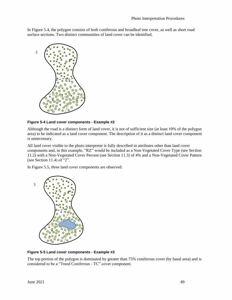
Photo Interpretation Procedures
June 2021 49
In Figure 5.4, the polygon consists of both coniferous and broadleaf tree cover, as well as short road
surface sections. Two distinct communities of land cover can be identified.
Figure 5-4 Land cover components - Example #2
Although the road is a distinct form of land cover, it is not of sufficient size (at least 10% of the polygon
area) to be indicated as a land cover component. The description of it as a distinct land cover component
is unnecessary.
All land cover visible to the photo interpreter is fully described in attributes other than land cover
components and, in this example, “RZ” would be included as a Non-Vegetated Cover Type (see Section
11.2) with a Non-Vegetated Cover Percent (see Section 11.3) of 4% and a Non-Vegetated Cover Pattern
(see Section 11.4) of “2”.
In Figure 5.5, three land cover components are observed.
Figure 5-5 Land cover components - Example #3
The top portion of the polygon is dominated by greater than 75% coniferous cover (by basal area) and is
considered to be a “Treed Coniferous - TC” cover component.
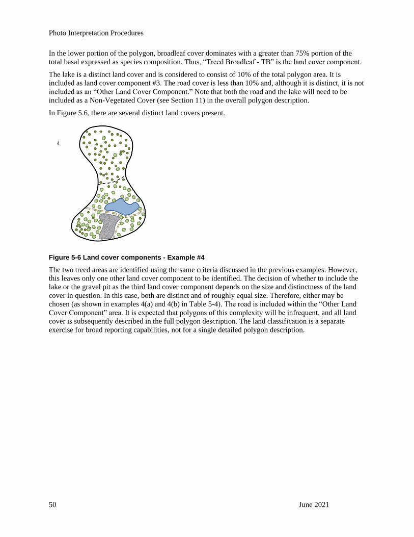
Photo Interpretation Procedures
50 June 2021
In the lower portion of the polygon, broadleaf cover dominates with a greater than 75% portion of the
total basal expressed as species composition. Thus, “Treed Broadleaf - TB” is the land cover component.
The lake is a distinct land cover and is considered to consist of 10% of the total polygon area. It is
included as land cover component #3. The road cover is less than 10% and, although it is distinct, it is not
included as an “Other Land Cover Component.” Note that both the road and the lake will need to be
included as a Non-Vegetated Cover (see Section 11) in the overall polygon description.
In Figure 5.6, there are several distinct land covers present.
Figure 5-6 Land cover components - Example #4
The two treed areas are identified using the same criteria discussed in the previous examples. However,
this leaves only one other land cover component to be identified. The decision of whether to include the
lake or the gravel pit as the third land cover component depends on the size and distinctness of the land
cover in question. In this case, both are distinct and of roughly equal size. Therefore, either may be
chosen (as shown in examples 4(a) and 4(b) in Table 5-4). The road is included within the “Other Land
Cover Component” area. It is expected that polygons of this complexity will be infrequent, and all land
cover is subsequently described in the full polygon description. The land classification is a separate
exercise for broad reporting capabilities, not for a single detailed polygon description.
Photo Interpretation Procedures
June 2021 51
6 Site Index Attributes
6.1 Introduction
All polygons with trees and polygons that are potentially capable of producing trees are to be assigned
site index values. Values are entered for the following attributes.
Estimated Site Index Species: species upon which the site index is based.
Estimated Site Index: site index in metres at base age 50 at DBH.
Estimated Site Index Source: the source of information for site index determination.
Photo interpreters will NOT be responsible for estimating values in the following situations:
• Polygons with trees 30 years old or greater (the site index for these stands will be derived from
the tree attributes)
• Regenerated stands located in silviculture openings, where the site index is present, attributes will
be obtained from silviculture field surveys unless declared free growing, and the interpreter
determines that the trees are suppressed and do not reflect the potential site productivity.
Photo interpreters will be responsible for estimating values in the following situations:
• Polygons with trees less than 30 years old (total age). Layers consisting of live or dead trees less
than 30 years require an estimated site index
• Polygons not in silviculture openings, with no tree cover at present, but estimated to be
potentially capable of producing trees if converted to a tree crop
• Polygons occupied by trees planted outside their normal ecological range or are occupied by
suppressed trees that do not reflect the potential site productivity of the polygon
The following sections describe the process of estimating site index values. For more information on site
index derivation, see Section 12 Derived Attributes.
6.2 Estimated Site Index Species
6.2.1 Definition
The estimated site index species are the tree species from which the site index for the polygon is derived.
6.2.2 Purpose
The estimate of site index species provides a link between the site index and particular tree species site
productivity (i.e., age/height curve).
6.2.3 Procedure
The interpreter will enter the site index species for:
• Polygons with trees less than 30 years (total age)
• Polygons currently non-treed but capable of producing trees (including completely dead stands)
• Polygons occupied by trees that have been planted outside their normal ecological range or
occupied by suppressed trees that do not reflect the potential site productivity of the polygon

Photo Interpretation Procedures
52 June 2021
The interpreter will view the polygon and select the tree species providing the best description of site
productivity:
• From the existing tree species
• From adjacent, similar stands
• From an assessment of ecological factors
• From ground information calibration points
6.3 Estimated Site Index
6.3.1 Definition
Estimated site index is an estimate of site productivity for tree growth (height in metres at breast height
age of 50 years).
6.3.2 Purpose
The estimated site index provides an estimate of the site productivity for tree species growth.
6.3.3 Procedure
Estimated site index may be based on the direct application of conventional site index curves, or it may be
estimated from other data sources. The direct site index value may be determined from the dominant and
codominant trees.
Note: Dominant trees have crowns receiving full light from above and full to partial light from the side.
Codominant trees have crowns receiving full light from above and comparatively little direct light
from the sides.
Alternative data sources may be used when assigning an estimated site index to:
• Young stands less than 30 years (total age)
• Polygons that are occupied by trees that have been planted outside of their normal ecological
range or occupied by suppressed stands that do not reflect their potential site productivity
• Non-treed areas with or without shrub or tree cover upon which it is estimated that a tree crop
could be produced.
For each category listed above, determine the most appropriate method for deriving site index.
Estimated site index is recorded to the nearest one metre.
Example:
Burned lodgepole pine area with no current tree coverage (interior stand).
Delineate denuded area (e.g., burn) into areas of similar productivity.
The estimated site index source code (for this example) is "E" Ecological Correlations (see following
Estimated Site Index Source).
Using Figure 6.1, establish the polygon's relevant slope position from which the site index can be
interpreted. When the polygon is in the receiving zone, the site index value is interpreted as 15 m.
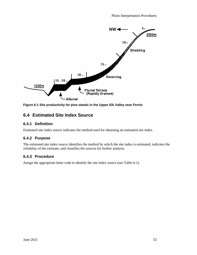
Photo Interpretation Procedures
June 2021 53
Figure 6-1 Site productivity for pine stands in the Upper Elk Valley near Fernie
6.4 Estimated Site Index Source
6.4.1 Definition
Estimated site index source indicates the method used for obtaining an estimated site index.
6.4.2 Purpose
The estimated site index source identifies the method by which the site index is estimated, indicates the
reliability of the estimate, and classifies the sources for further analysis.
6.4.3 Procedure
Assign the appropriate letter code to identify the site index source (see Table 6-1).
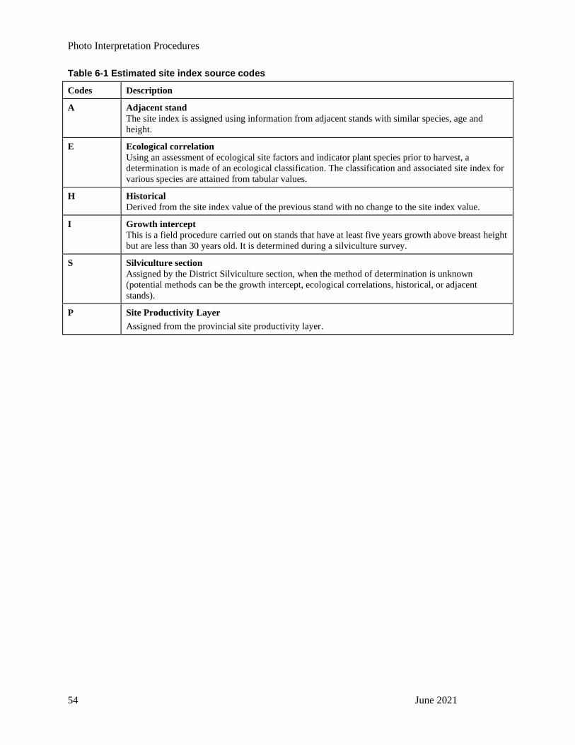
Photo Interpretation Procedures
54 June 2021
Table 6-1 Estimated site index source codes
Codes Description
A Adjacent stand
The site index is assigned using information from adjacent stands with similar species, age and
height.
E Ecological correlation
Using an assessment of ecological site factors and indicator plant species prior to harvest, a
determination is made of an ecological classification. The classification and associated site index for
various species are attained from tabular values.
H Historical
Derived from the site index value of the previous stand with no change to the site index value.
I Growth intercept
This is a field procedure carried out on stands that have at least five years growth above breast height
but are less than 30 years old. It is determined during a silviculture survey.
S Silviculture section
Assigned by the District Silviculture section, when the method of determination is unknown
(potential methods can be the growth intercept, ecological correlations, historical, or adjacent
stands).
P Site Productivity Layer
Assigned from the provincial site productivity layer.

Photo Interpretation Procedures
June 2021 55
7 Tree Attributes
7.1 Introduction
Tree attributes are layer-specific polygon estimates. The polygon is uniquely identified, and subsequent
qualitative and quantitative measurements are made for the tree cover in each layer of the polygon.
For normal aerial imagery, it is expected that estimation quality assurance of tree attributes would be
performed at the largest ground scale of approximately 1:3,000 in order to maintain consistency between
interpreters and for Quality Assurance purposes. This may be modified on a project-specific basis.
In cases where there is a discrepancy in photo estimation between the photo interpreter and Quality
Assurance personnel, the Quality Assurance personnel will adjust the viewing to a larger scale in order to
better assess the original estimate.
This section describes the process for developing estimates for polygon attributes related to tree cover.
These attributes are:
• Tree cover pattern
• Tree crown closure
• Tree layer
• Vertical complexity
• Species composition
• Age (leading and second species)
• Height (leading and second species)
• Update year
• Basal area
• Density
• Snag frequency
Attribution procedures for edge tying attributes
The interpreter may be instructed to join attributes between currently ongoing projects or older projects
completed in previous years (edge ties). Typically, interpreters will only tie to inventories completed to
the current VRI standard, but decisions on whether to tie to adjacent projects will be determined by the
Ministry on a contract-specific basis.
Attributes from adjacent projects should be carried over unless otherwise stated in the contract; however,
it is the interpreter’s responsibility to ensure attributes meet VRI standards.
When an interpreter is to edge tie attributes to another project, all attributes must match exactly, with a
number of exceptions:
• The types stop at the project boundary – this may occur at cutblock edges that end at a TSA or
TFL boundary, where the line separating two adjacent polygons will stop at a cutblock boundary
that happens to be on the edge of the project.
Photo Interpretation Procedures
56 June 2021
• A significant change has occurred between the two projects. Examples include insect outbreaks or
wildfires that occurred after the adjacent inventory was completed and prior to the imagery being
taken in the current inventory.
• The attributes on the adjacent inventory are clearly incorrect. Minor differences should still be
tied as is.
• New Silviculture opening information is available. The attributes will be updated to reflect new
RESULTS data even if it creates an edge tie mismatch.
Edge ties between individual submissions in a project should follow the same guidelines, but where the
difference is because one side is “clearly incorrect” polygons must be corrected on both sides of the edge
tie.
Usually, the edge of files delivered as a final product will follow mapsheet neatlines.
It is the interpreter’s responsibility to ensure that edge ties make sense as per the existing photos and data
supplied to support the contract.
7.2 Tree Cover Pattern
7.2.1 Definition
Tree cover pattern describes the spatial distribution of the tree cover within each tree layer in the polygon.
7.2.2 Purpose
Tree cover pattern is used to describe the tree layer spatial distribution. Examples include treed islands in
the subalpine parkland, clumps of trees on rocky outcrops, scattered groves or individual trees in an
otherwise shrubby flood plain or solid, continuous tree cover. Tree cover pattern provides information on
the amount of "edge" and "interior" habitat within the polygon.
7.2.3 Procedure
Enter the cover pattern code (1-9), from Appendix B, for the tree cover observed within the polygon.
Cover pattern is based on the majority area coverage.
Cover pattern is estimated for each tree layer in the polygon. It may help to visualize all the trees without
the aid of a stereoscope and interpret the cover pattern in this manner.
7.3 Tree Crown Closure
7.3.1 Definition
Tree crown closure is the percentage of ground area covered by the vertically projected crowns of the tree
cover for each tree layer within the polygon.
7.3.2 Purpose
Tree crown closure provides an essential estimate of the vertical projection of tree crowns upon the
ground. Since tree crown closure is very difficult to measure on the ground, this estimation by the
interpreter is important.

Photo Interpretation Procedures
June 2021 57
7.3.3 Procedure
Record crown closure to the nearest percent for the polygon. Where vegetation is overlapping (such as a
two-layer stand), only the visible portion of each layer is estimated for crown closure.
Crown closure is estimated for each tree layer in the polygon.
Crown closure estimation can be aided by:
• Cover comparison charts
Using a stereoscope to view the imagery, select a representative part of the polygon. Compare the
relative crown densities of the comparison chart (see Appendix C) against the representative crown
closure of the polygon. Select a relative crown density that most closely matches the polygon. Read
and enter the crown closure percent from the comparison chart.
• Black and White Stereogram Handbook and Colour Stereogram Handbook
These handbooks have photo examples with measured crown closure values. They include 70 mm
photo samples and measured photo samples that can be used as calibration values.
7.4 Tree Layer
7.4.1 Definition
Tree layer is a number that identifies the tree layer being described in a multi-layered stand.
7.4.2 Purpose
The tree layer identification creates a link between each polygon attribute and the corresponding tree
layer.
7.4.3 Procedure
Tree layers are distinguished according to recognized height differences which are, in many cases,
associated with distinct age differences. Identification guidelines may vary, depending on each user's
needs and the complexity of the project area. For example, trees from the former stand may be identified
as a layer with less than 5% crown closure. An example of this is a regenerated lodgepole pine stand
growing under an older Douglas-fir layer after a fire.
Enter a number to identify the tree layer being described. The layer of greatest height is indicated by "1",
and each subsequent height layer is identified with a larger number (e.g. the next greatest height would be
"2", the next greatest would be "3", etc.).
To be classified as multi-layered, a stand should meet the following criteria:
• Each layer must be distinct throughout the type
• Each layer should consist of different tree species except when the layer separation is distinct
• Differences in age and height between layers should be identifiable on the imagery and on the
ground
• Layers should differ by 40 years in age and 10 m in height. (Note: Silviculture layers that are
provided from RESULTS may not follow this convention. This is acceptable.)
• The bottom layer is usually established following a major disturbance such as fire or logging
Examples of multi-layered stands are shown in Appendix A.

Photo Interpretation Procedures
58 June 2021
Any stand that has more than an estimated 100 sph mortality would have a dead layer interpreted and is
identified with the layer code of “D.” Only one dead layer (D layer) is to be collected for each stand,
incorporating the dead even if they would have been collected as separate layers if they were alive. A tree
is considered “dead” for the purposes of the VRI if it has no foliage (seasonally dependent for deciduous
and Larch) or if all the foliage has the visible colour that is appropriate for a dead tree of that species.
The only attributes to be collected for a dead layer include the species composition, age of the leading
species, the height of the leading species, basal area, stems/ha and a data source code for each.
Requirements for the recording of each attribute are located in the sections below. An appropriate
disturbance code should also be collected where observed.
Site index attributes must be entered for all polygons with only a dead layer. Since these polygons are
non-treed but capable of producing trees, estimated site index is required as per Section 6.2.3 – Site Index
Attributes. (This may need a layer 1 for site index accessibility)
7.5 Vertical Complexity
7.5.1 Definition
Vertical complexity is a subjective classification that describes the form of each tree layer as indicated by
the relative uniformity of the forest canopy as it appears on aerial imagery. Vertical complexity is
influenced by stand age, species (succession as it relates to shade tolerance), and degree and age of past
disturbance. The tree height range is calculated as the total difference in height between the tallest and
shortest visible dominant, codominant, and high intermediate trees. To most adequately represent the tree
layer of interest, occasional occurrences of either very tall or very short trees should be ignored so that the
vertical complexity indicated is for the majority of stems in the dominant, codominant, and high
intermediate portion of each tree layer.
7.5.2 Purpose
Vertical complexity is used to identify and describe even-aged and uneven-aged stands for further
analysis in forest stand management and wildlife habitat assessment.
7.5.3 Procedure
Select the most appropriate code from Table 7-1 to best describe the vertical complexity for each tree
layer in the polygon.
Example Calculation:
The following is an example of the calculation to determine the percent difference in tree height for the
assignment of the Tree Vertical Complexity code. The Leading Species Height (dominant, codominant,
and high intermediate trees) is 23 m, and the tree heights range from 20 m to 26 m (all species in the
dominant, codominant, and high intermediate crown positions) for a total tree height range of 6 m:
Percent difference = Tree height range ÷ Height of leading species × 100 = 6 ÷ 23 × 100 = 26%
A difference of 26% correlates to a vertical complexity code 3 for the tree layer.
Notwithstanding the calculations above, plantations and young, immature stands less than 30 years of age
must be recorded with a vertical complexity code of 1.

Photo Interpretation Procedures
June 2021 59
Table 7-1 Coding for vertical complexity
Codes Description
1 Very uniform
A very uniform canopy with less than 11% difference between the height of the leading species and
the average tree layer height. Holes (or canopy gaps) are generally not visible in the canopy, and
there is usually no evidence on the imagery of recent disturbances affecting the form of the stand.
Examples include plantations and young, immature stands of shade-intolerant species.
2 Uniform
A uniform canopy with 11% - 20% difference between the height of the leading species and the
average tree layer height. A few holes (or canopy gaps) may be visible in the canopy, and there is
usually little or no evidence on the imagery of recent disturbance affecting the form of the stand.
3 Moderately uniform
A moderately uniform canopy with 21% - 30% difference between the height of the leading species
and the average tree layer height. Some holes (or canopy gaps) may be visible in the canopy, and
there may be evidence of past disturbance affecting the form of the stand. Stocking may be
somewhat patchy or irregular. Examples include older spruce-balsam stands.
4 Non-uniform
A relatively non-uniform canopy with 31% - 40% difference between the height of the leading
species and the average tree layer height. Holes (or canopy gaps) are often visible in the canopy (due
to past disturbance), and stocking is typically patchy or irregular.
5 Very non-uniform
A very non-uniform canopy with more than a 40% difference between the height of the leading
species and the average tree layer height. Stocking is typically very patchy or irregular. Examples
include disturbed dry belt Douglas-fir stands and decadent, coastal over-mature stands.
Example:
Average Tree Tree Height Range (m) by Vertical Complexity Code
Layer Height (m) 1 2 3 4 5
10 0 - 1.0 1.1 - 2.0 2.1 - 3.0 3.1 - 4.0 > 4.0
20 0 - 2.0 2.1 - 4.0 4.1 - 6.0 6.1 - 8.0 > 8.0
30 0 - 3.0 3.1 - 6.0 6.1 - 9.0 9.1 - 12.0 > 12.0
40 0 - 4.0 4.1 - 8.0 8.1 - 12.0 12.1 - 16.0 > 16.0
50 0 - 5.0 5.1 - 10.0 10.1 - 15.0 15.1 - 20.0 > 20.0
7.6 Species Composition
7.6.1 Definition
Species composition describes the tree species present and provides an estimate of the percentage of each
species within the polygon. Species percent is an estimate of the percentage of live tree species occupying
the polygon, based on the proportion of basal area or density (stands less than 2 metres).

Photo Interpretation Procedures
60 June 2021
7.6.2 Purpose
Species composition describes the various species of live trees that may be present in the polygon and
provides an estimate of the percentage of each species to the nearest percent. Species composition can be
used for volume derivation.
7.6.3 Procedure
Identify the tree species present in the polygon and list them in descending order. Up to six different
species may be identified. Estimate species composition for each tree layer in the polygon.
For each species identified, estimate the species composition to the nearest one percent for all living trees
of that species in the polygon based on density or basal area occupancy.
• When the height of the dominant, codominant and high intermediate trees is greater than or equal
to two metres, the estimate is based on basal area occupancy (square metres per hectare).
• When the height of the dominant, codominant and high intermediate trees is less than two metres,
the estimate is based on density (stems per hectare).
Note: Dominant trees have well-developed crowns that extend above the general level of the trees
around them. Codominant trees have crowns forming the general level of trees around them. High
intermediate trees have smaller crowns slightly below but extending into the general level of trees
around them.
The interpreter normally estimates the overall stand basal area first. Then this value is split into individual
estimates for each species. Species composition based on basal area is strongly correlated with species
composition based on volume. Studies have shown that volume and basal area correspond quite well,
except for some species. Cedar has a larger basal area in proportion to its volume, and spruce has a
smaller basal area in proportion to its volume.
The tools used to make these interpretations are stereograms, ground calibration points, ecological site
descriptions, and local knowledge. These interpretations are tempered by the knowledge of species
heights, crown shapes, and other factors.
Species composition must add up to 100%.
Species composition for dead layers may be difficult to estimate. The interpreter will use clues such as
existing known outbreaks of insects (species-specific), surrounding stands, BEC zones, historical
inventory data and other information to help determine species of dead stands.
It is important to establish the correct percentages for the leading species, as the stand age, height, and
site index are usually determined from the leading species.
In some instances, the interpreter will be able to identify the genera (e.g. Abies) but not be able to identify
the specific species (e.g. Abies amabalis or Abies grandis). In these instances, only the genera should be
identified. The level of identification may vary depending on the user's needs and the complexity of the
project area. The objective of the inventory is to identify the species accurately, wherever possible.
Acceptable genus and species codes are listed in Table 7-2 as summarized in version 4.5 of the 2009 BC
Ministry of Forests and Range Tree Code List.
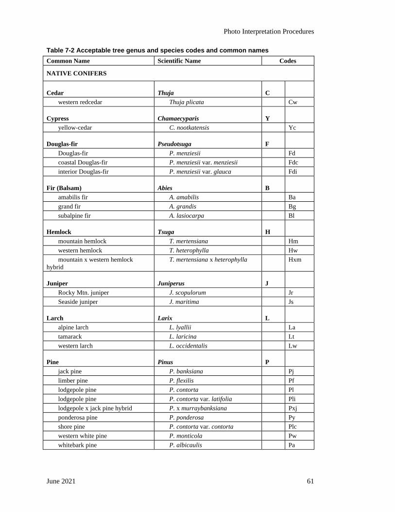
Photo Interpretation Procedures
June 2021 61
Table 7-2 Acceptable tree genus and species codes and common names
Common Name Scientific Name Codes
NATIVE CONIFERS
Cedar Thuja C
western redcedar Thuja plicata Cw
Cypress Chamaecyparis Y
yellow-cedar C. nootkatensis Yc
Douglas-fir Pseudotsuga F
Douglas-fir P. menziesii Fd
coastal Douglas-fir P. menziesii var. menziesii Fdc
interior Douglas-fir P. menziesii var. glauca Fdi
Fir (Balsam) Abies B
amabilis fir A. amabilis Ba
grand fir A. grandis Bg
subalpine fir A. lasiocarpa Bl
Hemlock Tsuga H
mountain hemlock T. mertensiana Hm
western hemlock T. heterophylla Hw
mountain x western hemlock
hybrid
T. mertensiana x heterophylla Hxm
Juniper Juniperus J
Rocky Mtn. juniper J. scopulorum Jr
Seaside juniper J. maritima Js
Larch Larix L
alpine larch L. lyallii La
tamarack L. laricina Lt
western larch L. occidentalis Lw
Pine Pinus P
jack pine P. banksiana Pj
limber pine P. flexilis Pf
lodgepole pine P. contorta Pl
lodgepole pine P. contorta var. latifolia Pli
lodgepole x jack pine hybrid P. x murraybanksiana Pxj
ponderosa pine P. ponderosa Py
shore pine P. contorta var. contorta Plc
western white pine P. monticola Pw
whitebark pine P. albicaulis Pa
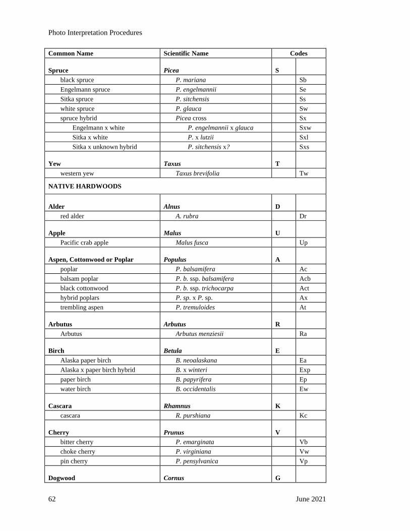
Photo Interpretation Procedures
62 June 2021
Common Name Scientific Name Codes
Spruce Picea S
black spruce P. mariana Sb
Engelmann spruce P. engelmannii Se
Sitka spruce P. sitchensis Ss
white spruce P. glauca Sw
spruce hybrid Picea cross Sx
Engelmann x white P. engelmannii x glauca Sxw
Sitka x white P. x lutzii Sxl
Sitka x unknown hybrid P. sitchensis x? Sxs
Yew Taxus T
western yew Taxus brevifolia Tw
NATIVE HARDWOODS
Alder Alnus D
red alder A. rubra Dr
Apple Malus U
Pacific crab apple Malus fusca Up
Aspen, Cottonwood or Poplar Populus A
poplar P. balsamifera Ac
balsam poplar P. b. ssp. balsamifera Acb
black cottonwood P. b. ssp. trichocarpa Act
hybrid poplars P. sp. x P. sp. Ax
trembling aspen P. tremuloides At
Arbutus Arbutus R
Arbutus Arbutus menziesii Ra
Birch Betula E
Alaska paper birch B. neoalaskana Ea
Alaska x paper birch hybrid B. x winteri Exp
paper birch B. papyrifera Ep
water birch B. occidentalis Ew
Cascara Rhamnus K
cascara R. purshiana Kc
Cherry Prunus V
bitter cherry P. emarginata Vb
choke cherry P. virginiana Vw
pin cherry P. pensylvanica Vp
Dogwood Cornus G

Photo Interpretation Procedures
June 2021 63
Common Name Scientific Name Codes
Pacific dogwood Cornus nuttallii Gp
Maple Acer M
bigleaf maple A. macrophyllum Mb
vine maple A. circinatum Mv
Oak Quercus Q
Garry oak Q. garryana Qg
UNKNOWNS
Unknown X
Unknown conifer Xc
Unknown hardwood Xh
EXOTICS
Apple Malus U
apple Malus pumila Ua
Aspen, Cottonwood or Poplar Populus A
*southern cottonwood P. deltoides Ad
Birch Betula E
European birch B. pendula Ee
silver birch B. pubescens Es
*yellow birch B. alleghaniensis Ey
Cherry Prunus V
sweet cherry P. avium Vs
Cypress Chamaecyparis Y
*Port Orford-cedar C. lawsoniana Yp
Fir (Balsam) Abies B
*balsam fir A. balsamea Bb
noble fir A. procera Bp
*Shasta red fir A. magnifica var. shastensis Bm
*white fir A. concolor Bc
Larch Larix L
*Dahurian larch L. gmelinii Ld
*Siberian larch L. siberica Ls
Maple Acer M
box elder A. negundo Me
*Norway maple A. platanoides Mn
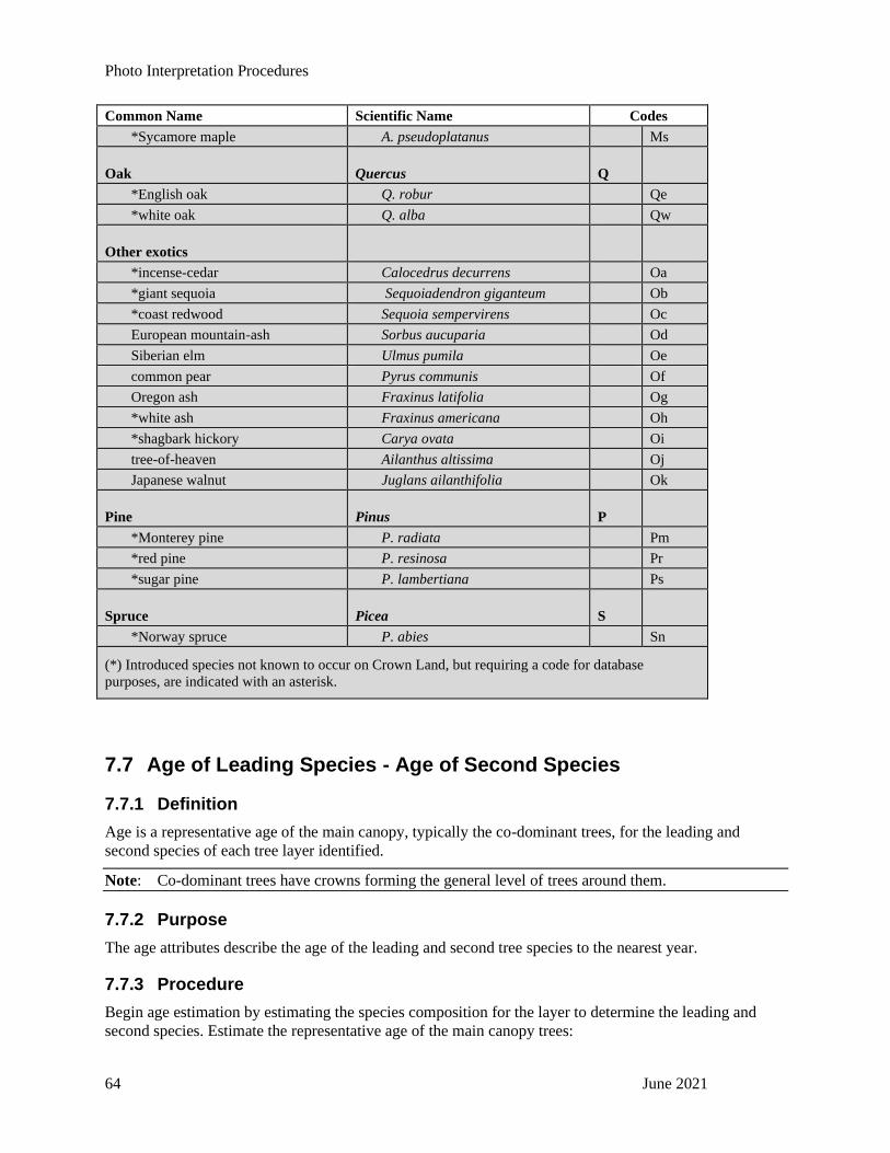
Photo Interpretation Procedures
64 June 2021
Common Name Scientific Name Codes
*Sycamore maple A. pseudoplatanus Ms
Oak Quercus Q
*English oak Q. robur Qe
*white oak Q. alba Qw
Other exotics
*incense-cedar Calocedrus decurrens Oa
*giant sequoia Sequoiadendron giganteum Ob
*coast redwood Sequoia sempervirens Oc
European mountain-ash Sorbus aucuparia Od
Siberian elm Ulmus pumila Oe
common pear Pyrus communis Of
Oregon ash Fraxinus latifolia Og
*white ash Fraxinus americana Oh
*shagbark hickory Carya ovata Oi
tree-of-heaven Ailanthus altissima Oj
Japanese walnut Juglans ailanthifolia Ok
Pine Pinus P
*Monterey pine P. radiata Pm
*red pine P. resinosa Pr
*sugar pine P. lambertiana Ps
Spruce Picea S
*Norway spruce P. abies Sn
(*) Introduced species not known to occur on Crown Land, but requiring a code for database
purposes, are indicated with an asterisk.
7.7 Age of Leading Species - Age of Second Species
7.7.1 Definition
Age is a representative age of the main canopy, typically the co-dominant trees, for the leading and
second species of each tree layer identified.
Note: Co-dominant trees have crowns forming the general level of trees around them.
7.7.2 Purpose
The age attributes describe the age of the leading and second tree species to the nearest year.
7.7.3 Procedure
Begin age estimation by estimating the species composition for the layer to determine the leading and
second species. Estimate the representative age of the main canopy trees:

Photo Interpretation Procedures
June 2021 65
• For the leading species, in each tree layer identified
• For the second species, in each tree layer identified
Recall that species composition is determined on the basis of basal area or density (see Section 7.6).
Figure 7.1 illustrates the selection of appropriate sample trees for age and height estimations.
Table 7-3 Crown class codes
Codes Description
D Dominant
Trees with crowns that extend above the general level of the trees immediately around the
measured trees. They are somewhat taller than the co-dominant trees and have well-
developed crowns, which may be somewhat crowded on the sides, receiving full light from
above and partly from the side.
C Co-dominant
Trees with crowns forming the general level of the trees immediately around the measured
trees. The crown is generally smaller than those of the dominant trees and is usually more
crowded on the sides, receiving full light from above and little from the sides.
I Intermediate
Trees with crowns below, but extending into, the general level of the trees immediately
around the measured trees. The crowns are usually small and quite crowded on the sides,
receiving little direct light from above but none from the sides.
S Suppressed
Trees with crowns entirely below the general level of the trees around the measured trees,
receiving no direct light either from above or from the sides.

Photo Interpretation Procedures
66 June 2021
Figure 7-1 Selection of appropriate sample trees for age and height estimations
Note: Third figure is a selectively logged interior dry belt stand. Arrows indicate trees included for age (and height) estimation.
The following data can be collected and used to aid in the photo-interpretation of tree age within a
polygon:
• History of origin (previous surveys, silviculture)
• Field measurements (for calibration, verification)
• Age-height-site relationships
• Age patterns
Any dead layer contained in the polygon will only require the age of the leading species to be recorded.
This age will be the representative age of ALL dead trees visible in the stand. As the aids listed in table
7.3 may not all be visible to the interpreter for a dead layer, the interpreter may need to use the

Photo Interpretation Procedures
June 2021 67
surrounding or remnant stand as a surrogate for age for the dead layer, keeping in mind obvious
differences in heights for much older “veterans.” Other aids are shown in Table 7-3 below.
Table 7-3 Aids to photo interpretation of age
Photo Characteristics Immature Mature
Stand texture Even Coarse (often crown openings are present)
Crown size on species Narrow Wide (varies dependent on species)
Height (height variation) Minor Variable
Height (size) Less than maximum Equals maximum per site
Snag frequency Few Increasing
Presence and height of
successional species
None Common, one example is spruce under aspen
Presence of short-lived
pioneer species
Present Reduced occurrence around 120 years.
Examples:
History of origin: A large wildfire in 1938. The ages of successional stands should be consistent
throughout the burn.
Figure 7-2 The use of historical information for age determination
7.8 Height of Leading Species - Height of Second Species
7.8.1 Definition
Height is a representative age of the main canopy, typically the co-dominant trees, for the leading and
second species of each tree layer identified.
Note: Codominant trees have crowns forming the general level of trees around them.

Photo Interpretation Procedures
68 June 2021
7.8.2 Purpose
An estimate of height is used to describe the height of the leading and second tree species to the nearest
tenth of a metre.
7.8.3 Procedure
Begin by estimating species composition for the tree layer to determine the leading and second species.
Estimate the representative height, to the nearest tenth of a metre, of the main canopy trees:
• For the leading species, in each tree layer identified
• For the second species, in each tree layer identified
Recall that species composition is determined on the basis of basal area or density (see Section 7.6).
Height adjustments
Consider making height adjustments for the following situations:
For species with narrow crowns as the crowns do not resolve on the imagery where the crown width is
less than one metre (e.g., narrow crowned alpine fir or rapidly growing coniferous). Heights may need to
be adjusted upward by 1 to 4 metres, depending on species and imagery resolution.
Figure 7-3 Resolution of tree crowns
For high-elevation stands, trees appear taller in imagery than they actually are because they are closer to
the aircraft camera. This may result in photo-interpreted heights being overestimated. When estimating
height, it is important to consider the effect of elevation changes and ecological factors on stand growth.
For example, trees growing in colder, drier conditions in the subalpine are generally shorter than trees
growing in a richer, wetter site in a valley bottom.
Any dead layer contained in the polygon will only require the height of the leading species to be
recorded. This height will be the average dominant, co-dominant and high intermediate height of ALL
dead trees visible in the stand. Resolution of the tops of dead trees will be especially difficult due to the
lack of foliage. The interpreter will usually need to adjust the dead tree height upwards to account for this
lack of resolution and use surrounding live trees/stands as an additional aid to interpretation.
AlpineFir
Spruce Aspen
Does not resolve
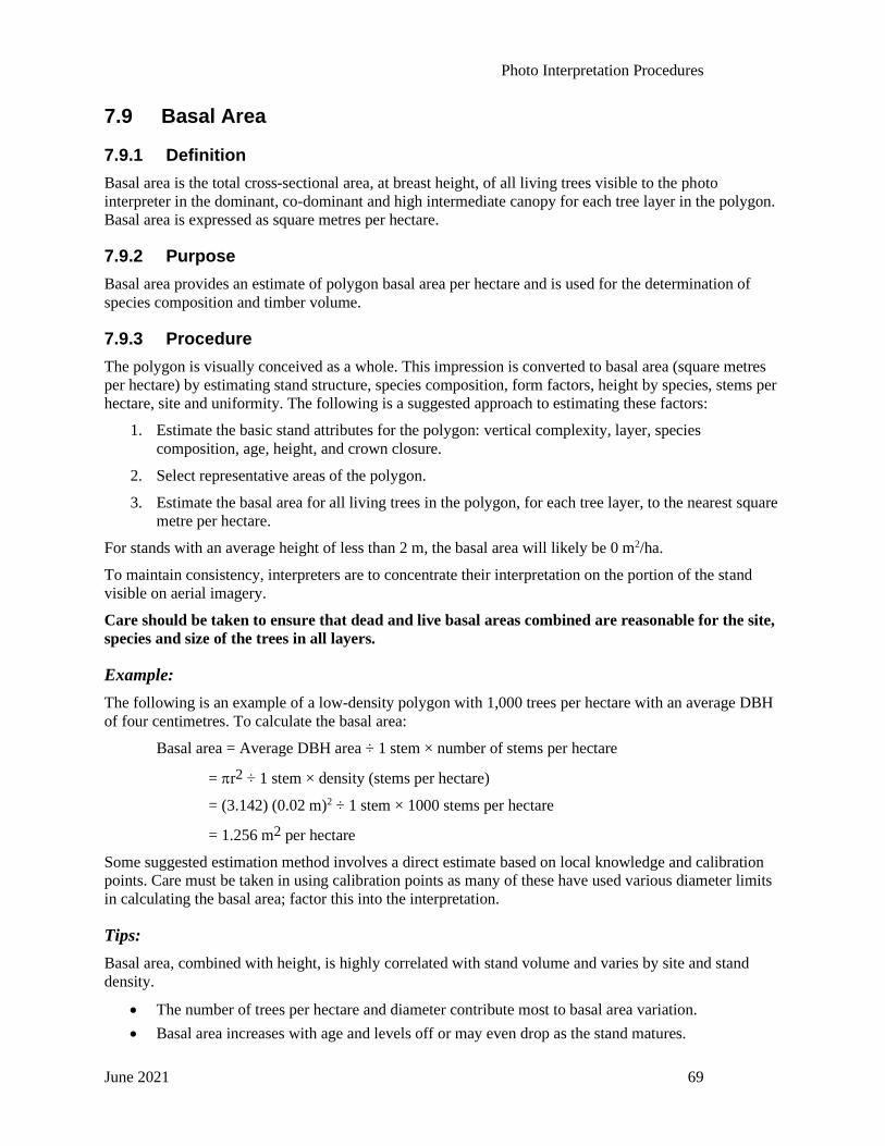
Photo Interpretation Procedures
June 2021 69
7.9 Basal Area
7.9.1 Definition
Basal area is the total cross-sectional area, at breast height, of all living trees visible to the photo
interpreter in the dominant, co-dominant and high intermediate canopy for each tree layer in the polygon.
Basal area is expressed as square metres per hectare.
7.9.2 Purpose
Basal area provides an estimate of polygon basal area per hectare and is used for the determination of
species composition and timber volume.
7.9.3 Procedure
The polygon is visually conceived as a whole. This impression is converted to basal area (square metres
per hectare) by estimating stand structure, species composition, form factors, height by species, stems per
hectare, site and uniformity. The following is a suggested approach to estimating these factors:
1. Estimate the basic stand attributes for the polygon: vertical complexity, layer, species
composition, age, height, and crown closure.
2. Select representative areas of the polygon.
3. Estimate the basal area for all living trees in the polygon, for each tree layer, to the nearest square
metre per hectare.
For stands with an average height of less than 2 m, the basal area will likely be 0 m2/ha.
To maintain consistency, interpreters are to concentrate their interpretation on the portion of the stand
visible on aerial imagery.
Care should be taken to ensure that dead and live basal areas combined are reasonable for the site,
species and size of the trees in all layers.
Example:
The following is an example of a low-density polygon with 1,000 trees per hectare with an average DBH
of four centimetres. To calculate the basal area:
Basal area = Average DBH area ÷ 1 stem × number of stems per hectare
= r2 ÷ 1 stem × density (stems per hectare)
= (3.142) (0.02 m)2 ÷ 1 stem × 1000 stems per hectare
= 1.256 m2 per hectare
Some suggested estimation method involves a direct estimate based on local knowledge and calibration
points. Care must be taken in using calibration points as many of these have used various diameter limits
in calculating the basal area; factor this into the interpretation.
Tips:
Basal area, combined with height, is highly correlated with stand volume and varies by site and stand
density.
• The number of trees per hectare and diameter contribute most to basal area variation.
• Basal area increases with age and levels off or may even drop as the stand matures.

Photo Interpretation Procedures
70 June 2021
7.10 Density
7.10.1 Definition
Density is the average number of living trees visible to the photo interpreter in the dominant, co-dominant
and high intermediate canopy for each tree layer in the polygon. Density is expressed as stems per
hectare.
7.10.2 Purpose
Density provides a direct estimate of tree stems per hectare.
7.10.3 Procedure
The following is a suggested approach to estimating density:
1. Estimate the basic stand attributes for the polygon: vertical complexity, layer, species
composition, age, height and crown closure.
2. Select representative areas of the polygon.
3. Estimate the density of trees in the polygon for each tree layer to the nearest stem per hectare
when practical.
The dead layer density must equal the VRI Snags Frequency for the entire polygon where a dead layer has
been recorded.
Some suggested methods of estimation are:
• Direct estimate: based on local field experience and photo calibration points. Care must be taken
in using calibration points as many of these have used various diameter limits in calculating tree
density; factor this into the interpretation.
• Indirect estimate: based on a comparison of the target area against a Ministry-verified
stereogram from the Black and White Stereogram Handbook or Colour Stereogram Handbook
that represents similar stand characteristics. Adjust the stereogram density to account for local
variations.
• Variable Density Yield Prediction (VDYP): for baseline estimates, compare the target area
against a VDYP predicted density for the species composition, age, site and crown closure.
Adjust the VDYP predicted density to account for local variations.
Note: Variable Density Yield Prediction is a method, based on empirical data, of calculating
mensurational data (primarily stand volume and tree diameter) from photo interpreted data (such
as species composition, basal area, age, height, crown closure).
7.11 Snag Frequency
7.11.1 Definition
Snag frequency is defined as the number of standing dead trees visible to the photo interpreter in the
dominant, co-dominant and high intermediate canopy for each tree layer. Snag frequency is expressed as
stems per hectare for each tree layer.

Photo Interpretation Procedures
June 2021 71
7.11.2 Purpose
The snag frequency provides a direct estimate of snags per hectare that can be used for wildlife and fire
management and provides information for danger tree assessment.
7.11.3 Procedure
The following is a suggested approach to estimating snag frequency:
1. Select representative areas of the polygon.
2. Estimate the number of snags per hectare for each tree layer in the polygon.
The Snag Frequency must equal the dead layer density for the entire polygon where a dead layer has been
recorded.
Note: Old-growth stands, particularly with cedar or cypress stems, may show numerous dead (whitish)
tops that will appear as snags but are actually living trees.
Photo Interpretation Procedures
72 June 2021
8 Shrub Attributes
8.1 Introduction
This set of attributes describes the portion of shrub cover within the polygon that is not obscured under
the vertical projection of tree crown cover. Shrubs are generally multi-stemmed or non-erect woody plant
species. Shrubs do not include species previously identified as trees or those low woody plants and
intermediate life forms referred to in Table 4.1 of Describing Ecosystems in the Field, H. Luttmerding et
al., MOE Manual 11, Dec. 1990.
8.2 Shrub Height
8.2.1 Definition
Shrub height is the average height, in tenths of a metre, of all shrubs within the polygon.
8.2.2 Purpose
Shrub height describes the average height of shrub species to the nearest tenth of a metre. When
multiplied by shrub cover, an index of shrub volume is obtained that indicates available browse.
8.2.3 Procedure
Estimate the average height in metres (weighted by crown closure) of all shrubs within the polygon that
are not obscured by tree crown cover.
Example:
Where you have two distinct shrub species, of two distinct heights, within one polygon:
Shrub Species Height Crown Closure
A 1.0 m 30%
B 5.0 m 20%
A, B weighted
average = 2.6 m 50%
Note: The height of shrubs less than 2.0 m is particularly important to wildlife and range managers as
this represents the critical threshold for the availability of browse.
8.3 Shrub Crown Closure
8.3.1 Definition
Shrub crown closure is the percentage of ground area covered by the vertically projected crowns of the
shrub cover visible to the photo interpreter. Shrub crown closure is expressed as a percentage of the entire
polygon.
Photo Interpretation Procedures
June 2021 73
8.3.2 Purpose
Shrub crown closure provides a direct photo estimate of crown cover.
8.3.3 Procedure
Estimate crown closure for all shrub species based on the percentage of ground area covered by the
vertically projected crowns of shrubs. Only those shrubs not otherwise obscured by tree crown cover are
recorded. Record the crown closure to the nearest percent. No overlap of vegetation is considered for
crown closure estimation.
Where different cover types occur, the following procedures may be used:
• Weight the crown closure estimate by the specific cover types. For example:
o Shrub land cover component (60% of area) has crown closure (CC) of 80% for shrubs
o Herb land cover component (40% of area) has crown closure of 10% for shrubs
• Therefore: (60% × 80% CC) + (40% × 10% CC) = 52% shrub crown closure for the polygon
The following methodology will assist in the estimation of shrub crown closure:
• Under stereoscopic viewing, select a representative part of the polygon
• Compare the relative crown densities of the cover comparison chart (see Appendix C) against
the representative crown closure of the polygon
• Select a relative crown density that most closely matches the polygon; enter the crown closure
percent from the comparison chart
8.4 Shrub Cover Pattern
8.4.1 Definition
Shrub cover pattern is a code that describes the spatial distribution of the shrubs within the polygon.
8.4.2 Purpose
Shrub cover pattern is used to describe the shrub layer spatial distribution. Examples include clumps of
shrubs on rocky outcrops, scattered patches or individual shrubs or solid, continuous shrub cover.
8.4.3 Procedure
Enter the cover pattern code (1-9) for shrub cover within the polygon from Appendix B. Shrub cover
pattern is based on the majority area coverage.


Photo Interpretation Procedures
June 2021 75
9 Herb Attributes
9.1 Introduction
This set of attributes describes the portion of herb cover that is not obscured by the vertical projection of
the crowns of either trees or shrubs.
Herbs are defined as non-woody (vascular) plants, including graminoids (sedges, rushes, grasses), forbs
(ferns, club mosses, and horsetails) and some low, woody species and intermediate life forms identified in
Table 4.1 of Describing Ecosystems in the Field, H. Luttmerding et al., MOE Manual 11, Dec. 1990.
9.2 Herb Cover Type
9.2.1 Definition
Herb cover types are the designations for herb-dominated areas as listed in the BC Land Cover
Classification Scheme.
9.2.2 Purpose
Herb cover types will provide detailed reporting for herbaceous land cover.
9.2.3 Procedure
Enter the appropriate code from Table 9-1 to the level of resolution that can be photo interpreted for all
herbaceous cover types observable in the polygon.
Table 9-1 Coding for herb cover type
Codes Description
HE Herb
A Herb polygon with no distinction between forbs and graminoids
HF Herb - Forbs
A Herb polygon with forbs greater than 50% of the herb cover.
HG Herb - Graminoids
A Herb polygon with graminoids greater than 50% of the herb cover.
9.3 Herb Cover Percent
9.3.1 Definition
Herb cover percent is the percentage of ground area covered by herbaceous cover visible to the photo
interpreter. Herb cover percent is analogous to tree and shrub crown closures and is expressed as a
percentage of the entire polygon.
9.3.2 Purpose
Herb cover percent provides a direct estimate of herbaceous cover.

Photo Interpretation Procedures
76 June 2021
9.3.3 Procedure
Estimate herbaceous cover based on the percentage of ground area covered by the herbs (see Appendix
C). Record herbaceous cover to the nearest percent.
9.4 Herb Cover Pattern
9.4.1 Definition
Herb cover pattern is a code that describes the spatial distribution of the herbaceous cover within a
polygon.
9.4.2 Purpose
Herb cover pattern is used to describe the herb layer spatial distribution. Examples include herbaceous
cover on rocky outcrops or patches of herbaceous cover within shrub-dominated polygons.
9.4.3 Procedure
Enter the cover pattern code (1-9) for herbaceous cover within the polygon, from Appendix B. Herb cover
pattern is based on the majority area coverage.

Photo Interpretation Procedures
June 2021 77
10 Bryoid Attributes
10.1 Introduction
This set of attributes describes the portion of bryoid cover that is not obscured by the vertical projection
of the crowns of trees, shrubs, or herbs.
Bryoids include mosses, liverworts, hornworts, and non-crustose lichens.
10.2 Bryoid Cover Percent
10.2.1 Definition
Bryoid cover percent is the percentage of ground area covered by bryoids visible to the photo interpreter.
Bryoid cover percent is expressed as a percentage of the entire polygon.
10.2.2 Purpose
Bryoid cover percent provides a direct estimate of bryoid cover.
10.2.3 Procedure
Estimate bryoid cover based on the percentage of ground area covered by bryoids that are not obscured by
taller life forms (see Appendix C). Record bryoid cover to the nearest percent.
Bryoids are typically found in abundance and/or dominating certain broad ecosystem units – i.e. high
elevation, rockier alpine areas, and wetlands with water-saturated soils. As such, bryoids will be more
abundant and identifiable in imagery for sparsely vegetated sites that tend to be drier or wetter – i.e. sites
with a soil moisture regime 0, 1, 2, 7 or 8.
Interpreters are expected to identify bryoids only if they can be viewed and identified in the imagery.


Photo Interpretation Procedures
June 2021 79
11 Non-Vegetated Attributes
11.1 Introduction
This set of attributes describes the portion of the polygon that is non-vegetated (vegetation cover is less
than 5% of the total surface area of the polygon) and is not obscured by vegetation or shadows.
11.2 Non-Vegetated Cover Type(s)
11.2.1 Definition
Non-vegetated cover types are the designations (from level 5 of the BC Land Cover Classification
Scheme) for all observable non-vegetated land cover within the polygon.
11.2.2 Purpose
Non-vegetated cover types provide detailed reporting for non-vegetated land cover.
11.2.3 Procedure
Enter the appropriate code (see Table 11-1) to the level of resolution that can be photo interpreted for all
non-vegetated cover types observable within the polygon. When more than one non-vegetated cover type
is identified, use additional rows on the attribute form or in the database, as required.
A maximum of five (5) non-vegetated attributes is acceptable per polygon.
BCLCCS Level 4 non-vegetated cover type codes SI (Snow/Ice), RO (Rock/Rubble), CL (Cultivated
Land) and EL (Exposed Land) are non-available descriptions for this attribute.
Table 11-1 Codes for non-vegetated cover
Codes Description
Land Cover
GL Glacier
A mass of perennial snow and ice with definite lateral limits, typically flowing in a particular
direction.
PN Snow Cover
Snow or ice that is not part of a glacier but is found during the summer months on the landscape.
(Care should be taken to determine if the snow on the imagery is a result of the photo acquisition
date. In such cases, the delineation or attribution procedure should be discussed with the Ministry).
BR Bedrock
Unfragmented consolidated rock, contiguous with underlying material.
TA Talus
Rock fragments of any size accumulated on or at the foot of slopes as a result of successive rock
falls. This is a type of colluvium.
BI Blockfield
Blocks of rock derived from the underlying bedrock by weathering and/or frost heaving. These have
not undergone any significant down slope movement as they occur on level or gently sloping areas.

Photo Interpretation Procedures
80 June 2021
Codes Description
MZ Rubbly Mine Spoils
Discarded overburden or waste rock, moved to extract ore during mining.
LB Lava Bed
An area where molten rock has flowed from a volcano or fissure and cooled and solidified to form
rock.
RS River Sediments
Silt, gravel and sand bars associated with former river channels and present river edges.
DW Downed Wood
Consolidated Coarse Woody Debris, Blowdown, Log Decks, Burn pile, or any area of downed trees.
ES Exposed Soil
Any exposed soil not covered by other categories such as areas of recent disturbance that include
mud slides, debris torrents, avalanches, or disturbances such as pipeline rights-of-way where
vegetation cover is less than five percent. Exposed soil resulting from harvesting operations is
recognized in this category; however, harvested polygons must maintain vegetated status.
LS Pond or Lake Sediments
Exposed sediments related to dried lakes or ponds.
RM Reservoir Margin
Land exposed by a drained or fluctuating reservoir. This is found above "normal" water levels and
may consist of a range of substrates, including gravel, cobbles, fine sediments, or bedrock.
BE Beach
An area with sorted sediments reworked in recent time by wave action which may be formed at the
edge of fresh or saltwater bodies
LL Landing
A compacted area adjacent to a road used for the purpose of sorting and loading logs.
BU Burned Area
Land showing evidence of recent burning, either natural or prescribed. Vegetation of less than 5%
crown cover is present at the time of polygon description.
RZ Road Surface
An area cleared and compacted for transporting goods and services by vehicles. Older roads that
appear vegetated and are used infrequently or not at all may cease to be considered a road surface.
MU Mudflat Sediment
Flat plain-like areas associated with lakes, ponds, rivers or streams - dominated by fine-textured
sediments. They can be associated with freshwater or estuarine sources.
CB Cutbank
Part of a road corridor created upslope of the road surface created by excavation into the hillside.
MN Moraine
An area of debris transported and deposited by a glacier.
GP Gravel Pit
An area exposed through the removal of sand and gravel.
TZ Tailings
An area containing the solid waste material produced in the mining and milling of ore.
RN Railway
A roadbed with fixed rails that may contain single or multiple rail lines.

Photo Interpretation Procedures
June 2021 81
Codes Description
UR Urban
Buildings and associated developments such as roads and parking areas which form an almost
continuous covering of the landscape.
AP Airport
A permanent, paved or gravel area, and associated buildings and parking used by airplanes.
MI Open Pit Mine
An exposed area used to extract ore during a mining operation. This may contain associated
buildings and any tailing produced by the mining and milling process.
OT Other
A non-vegetated polygon where none of the above categories can be reliably chosen. This code is
used very rarely.
Water Cover
LA Lake
A naturally occurring static body of water. The boundary for the lake is the natural high-water mark.
RE Reservoir
An artificial basin affected by impoundment behind a man-made structure such as a dam, berm,
dyke, or wall.
RI River/Stream
A watercourse formed when water flows between continuous, definable banks. Flow may be
intermittent or perennial but does not include ephemeral flow where a channel with no definable
banks is present. Gravel bars are part of a stream, while islands within a stream that has definable
banks are not.
OC Ocean
A naturally occurring body of water containing salt or generally considered to be salty.
11.3 Non-Vegetated Cover Percent
11.3.1 Definition
The non-vegetated cover percent indicates the percentage of polygon area occupied by a non-vegetated
cover.
11.3.2 Purpose
Non-vegetated cover percent provides a direct estimate of non-vegetated cover, which is not adjusted.
11.3.3 Procedure
Estimate non-vegetated cover percent, based on the percentage of the ground area of the polygon covered
by the non-vegetated cover type (see Appendix C). Enter the cover percent estimate on the same line of
the attribute form as the cover type.
Enter the non-vegetated cover percent for each non-vegetated cover type identified in the polygon. There
are no constraints to the number of non-vegetated cover types that can be identified.
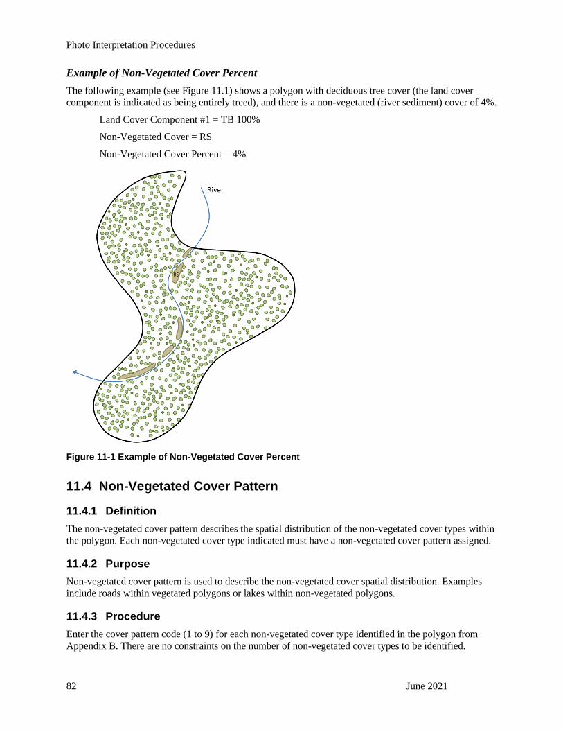
Photo Interpretation Procedures
82 June 2021
Example of Non-Vegetated Cover Percent
The following example (see Figure 11.1) shows a polygon with deciduous tree cover (the land cover
component is indicated as being entirely treed), and there is a non-vegetated (river sediment) cover of 4%.
Land Cover Component #1 = TB 100%
Non-Vegetated Cover = RS
Non-Vegetated Cover Percent = 4%
Figure 11-1 Example of Non-Vegetated Cover Percent
11.4 Non-Vegetated Cover Pattern
11.4.1 Definition
The non-vegetated cover pattern describes the spatial distribution of the non-vegetated cover types within
the polygon. Each non-vegetated cover type indicated must have a non-vegetated cover pattern assigned.
11.4.2 Purpose
Non-vegetated cover pattern is used to describe the non-vegetated cover spatial distribution. Examples
include roads within vegetated polygons or lakes within non-vegetated polygons.
11.4.3 Procedure
Enter the cover pattern code (1 to 9) for each non-vegetated cover type identified in the polygon from
Appendix B. There are no constraints on the number of non-vegetated cover types to be identified.

Photo Interpretation Procedures
June 2021 83
12 Disturbance Events Information
12.1 Definition
The Disturbance Events Information section describes any natural or human-caused event that has
impacted the land base and is represented in the polygon.
12.2 Purpose
Disturbance Event codes provide a detailed description of any event that has impacted the land base.
Some events can impact forests at the landscape level, such as a bark beetle epidemic and wildfires, while
other events are limited in extent, such as logging or flooding.
12.3 Procedure
A disturbance code must be assigned where an event is present on the land base. The most common
human-caused disturbance likely to be encountered within a VRI project area is logging. Disturbance
information may be found in the RESULTS data, the previous inventory and other data sources. The
interpreter will identify the disturbance code as Logging (L) but will also be expected to enter any
Disturbance Start and Disturbance End date provided in RESULTS. Start and End dates must consist of
Month/Day/Year. Refer also to Section 13 for further information on RESULTS coding.
Disturbance codes consist of a dichotomous hierarchy. When the interpreter has been provided
supplemental information or has conducted any ground-truthing, they must use a more descriptive sub-
category code to identify the specific forest damage agent. The first letter of each code is a general
description of a disturbance type, and subsequent letters in the code further describe the damage agent.
For example, the code for mountain pine beetle is IBM.
All disturbance types on the land base and their assigned codes can be found in the VRIMS Personal
Geodatabase Structure and Use manual.
In the case of natural disturbances, it may not be possible to determine a Start and End date, and those
fields should be left blank. Any supplemental information provided by the Ministry that has a start year
must be recorded, for example, Burn Years.
An interpreter may have to interpret polygons that have multiple types of disturbances. In these cases, it
will be up to the interpreter to determine which disturbance had the greater stand volume impact on the
land base and record the appropriate code.

Photo Interpretation Procedures
June 2021 85
13 RESULTS
13.1 Definition
The Reporting Silviculture Updates and Land Status Tracking System (RESULTS) tracks silviculture
information by managing the submission of openings, disturbances, silviculture activities and obligation
declarations as required by the Forest and Range Practices Act.
RESULTS data is collected by Resource Practices Branch and contains spatial and attribute data used for
tracking depletion (harvest), regeneration, silviculture reserves and free growing (FG). This and other data
sources are summarized by Forest Analysis and Inventory Branch for incorporation into new VRIs and
provided to interpreters in the ArcMap Personal Geodatabase (PGDB) format. In this document, the term
“RESULTS” refers to the Forest Analysis and Inventory Branch summarized version of this silviculture
data and other data sources.
The Ministry will supply a prepared RESULTS data package. This package consists of a single spatial
and attribute data file in a Vegetation Resources Inventory Management System (VRIMS) format, as well
as a point file containing the same attributes for integration into new inventories. The package reduces the
need for the interpreter to adjust opening boundaries and determine attributes from multiple sources.
The Ministry recommends the use of automated transfer techniques to import RESULTS spatial and
attribute data into the Contractor’s data set, followed by a thorough review of the transferred data.
13.2 RESULTS Openings and Polygon Delineation
The interpreter must consider a few guiding principles when integrating RESULTS data into a new VRI
photo interpretation project.
1. Provide reliable polygon forest cover descriptions based on the photo estimated vegetation
attributes and the supporting RESULTS information. The intent is not to make minor changes in
attributes from RESULTS; the intent is to correct for apparent errors that exist in the RESULTS
data when compared to what is observed on the imagery.
2. Review every opening to ensure that the final VRI polygon description is consistent with the
principles described in the VRI Photo Interpretation Procedures. The interpreter will discuss
proposed modifications of RESULTS data with the Ministry Representative before incorporation.
3. The Ministry has supplied the “SPATIAL_SOURCE” field in the RESULTS database, which
identifies the source of the spatial data for a particular opening. In general, openings with spatial
data identified as “FTEN_POLY” and “RESULTS_OPENING” will have lower qualities of
delineation and attribution data. These openings will likely require additional review and editing
than openings with a “RESULTS_FOREST_COVER” spatial data source.
4. Re-delineate RESULTS boundaries only when the Ministry-supplied delineation is greater than
20 m of the correct location viewed in the image. Thus, do not re-delineate if the interpreted
delineation based on what is observed on the imagery is less than 20 m of the Ministry-supplied
RESULTS delineation.
5. Maintain the opening boundaries and Opening IDs as supplied for openings created by single-tree
selection, salvage logging, multiple entry harvesting, or similar.

Photo Interpretation Procedures
86 June 2021
13.2.1 External Opening Boundaries
There are two types of boundaries of concern when incorporating RESULTS boundaries: external
boundaries, which form the outside edge of a cut block as determined by a unique Opening ID, and
internal boundaries, which differentiate between the different stand types.
The Ministry-supplied RESULTS layers have been reviewed for the spatial correctness of each opening
and include the removal of road tubes, overlaps and slivers. There will be situations where openings are
visible on the imagery, but the associated opening delineation and data may not be present in the
Ministry-supplied RESULTS dataset. Standard delineation procedures will apply for these openings.
Furthermore, there will be situations where harvesting occurred after imagery acquisition; that is, the
opening is not visible on the imagery. Where delineation and data exist in the Ministry-supplied
RESULTS dataset for an opening harvested after imagery acquisition (i.e. RESULTS Reference Year ≥
imagery acquisition date), use the RESULTS delineation and data for the opening as supplied with no
alteration.
There will be situations where what appears to be a single large opening is comprised of several unique
openings directly adjacent to each other, each with its disturbance or silviculture history. Figure 13-1 is an
example of this situation. Each opening is identified by a unique Opening ID number in the Ministry-
supplied RESULTS data. Ensure that each opening is assigned the correct RESULTS data.
Figure 13-1 Example of a Ministry-prepared RESULTS spatial layer with multiple openings
13.2.2 Internal Opening Boundaries
Internal polygon delineation requirements differ between openings that are declared Free Growing and
openings that are not declared Free Growing.
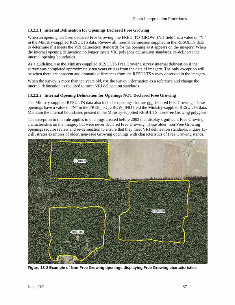
Photo Interpretation Procedures
June 2021 87
13.2.2.1 Internal Delineation for Openings Declared Free Growing
When an opening has been declared Free Growing, the FREE_TO_GROW_IND field has a value of “Y”
in the Ministry-supplied RESULTS data. Review all internal delineation supplied in the RESULTS data
to determine if it meets the VRI delineation standards for the opening as it appears on the imagery. When
the internal opening delineation no longer meets VRI polygons delineation standards, re-delineate the
internal opening boundaries.
As a guideline, use the Ministry-supplied RESULTS Free Growing survey internal delineation if the
survey was completed approximately ten years or less from the date of imagery. The only exception will
be when there are apparent and dramatic differences from the RESULTS survey observed in the imagery.
When the survey is more than ten years old, use the survey information as a reference and change the
internal delineation as required to meet VRI delineation standards.
13.2.2.2 Internal Opening Delineation for Openings NOT Declared Free Growing
The Ministry-supplied RESULTS data also includes openings that are not declared Free Growing. These
openings have a value of “N” in the FREE_TO_GROW_IND field the Ministry-supplied RESULTS data.
Maintain the internal boundaries present in the Ministry-supplied RESULTS non-Free Growing polygons.
The exception to this rule applies to openings created before 2003 that display significant Free Growing
characteristics on the imagery but were never declared Free Growing. These older, non-Free Growing
openings require review and re-delineation to ensure that they meet VRI delineation standards. Figure 13-
2 illustrates examples of older, non-Free Growing openings with characteristics of Free Growing stands.
Figure 13-2 Example of Non-Free Growing openings displaying Free Growing characteristics

Photo Interpretation Procedures
88 June 2021
13.3 RESULTS Openings and Polygon Attribution
The procedures for integrating RESULTS attribute data into a VRI photo interpretation project are:
1. Ministry-supplied RESULTS data has two layers of information for each opening polygon:
a. A point (centroid) layer set to an “I” (Incomplete) standard in the VRIMS
“INVENTORY_STANDARD_CODE” field; and
b. A polygon layer called the “FOREST_COVER_OBJECT” and associated VRIMS
attribute tables also set to the “I” standard for each RESULTS polygon
2. Each RESULTS opening is supplied with an attribute set that may or may not have a complete set
of RESULTS survey data. In general, openings identified as “FTEN_POLY” and
“RESULTS_OPENING” in the “SPATIAL_SOURCE” field of the Ministry-supplied RESULTS
data typically contain minimal attribute data and is often limited to an opening ID and logging
history date. More recent Free Growing openings typically have all the tree layer attributes from
the Free Growing survey, including species composition, age, height, density, site index, etc.
Review each opening to determine, using the VRI RESULTS standards and criteria, if the
opening requires attribution to the “I” or “V” standard. Details about the criteria used to
determine the attribution standard required are provided in the sections below.
3. Non-Free Growing openings may contain multiple layers in the Ministry-supplied RESULTS
data (i.e. RESULTS layers 1, 2, 3, 4, etc.). Incorporate all Ministry-supplied RESULTS layers
into any polygon identified as non-Free Growing. It is not acceptable to amalgamate multi-layer
RESULTS data into a reduced number of layers or exclude one or more RESULTS layers to
simplify the attribution. These layers may not meet the VRI layer definition as there may be only
slight differences between the age and height of the separate layers.
4. Free Growing openings may also contain multiple layers in the Ministry-supplied RESULTS
data. Using the RESULTS silviculture survey data as a guide, describe what is visible on the
imagery. This may modify the number of layers provided in the RESULTS data.
5. When trees are present in a polygon, describe each tree layer to VRI standards. Describe non-Free
Growing openings to the “I” standard and Free Growing openings to the “V” standard. Openings
identified as non-Free Growing in the Ministry-supplied RESULTS data that have significant
Free Growing characteristics (as with example Figure 13-2) are attributed to the “V” standard but
still retain an “N” value in the “FREE_TO_GROW_IND” field. Further details describing the
attribution requirements for “I” and “V” standards are provided in section 13.3.1.
6. Assign a crown closure to each layer in the polygon that will sum to a total of at least 11% for all
the tree layers combined to all openings where a tree layer is visible on the imagery or provided
by RESULTS, even when the opening appears on the imagery to have a crown closure less than
11%. Attribute openings with more than 11% crown closure, according to the crown closure
visible on the imagery.
7. The reference year is typically the year of the RESULTS data (i.e. survey year) when attributing
polygons with the Ministry-supplied RESULTS data. Use the year of imagery as the reference
year when a RESULTS opening is attributed to the “V” standard.
8. Use the site indices in the Ministry-supplied RESULTS data if they are a reasonable reflection of
what is observed on the imagery. When no site index is available, it is crucial to carefully use the
year of disturbance and reference year to derive the correct age together with a height
measurement or estimate to provide a true age/height relationship. Site index is an important
determinant of site productivity and informs future management options for that site or stand of
trees. Since predicting growth rates of young planted trees can be very difficult and site index
Photo Interpretation Procedures
June 2021 89
curves unreliable in the early stages of a stand, it is imperative that the age/height ratio is
estimated as accurately as possible to provide end-users with the best opportunity at predicting
site potential. This is particularly true of stands between 20 and 35 years that have been declared
Free Growing as they will have no further surveys completed.
9. Review each opening to ensure a correct Opening ID has been applied and review the
corresponding attributes for accuracy and completeness.
10. The existing forest cover inventory provided by the Ministry must be reviewed to obtain any
logging history or Opening IDs that are not present in the RESULTS data set provided. The
interpreter will delineate the boundary using VRI delineation standards and is responsible for
interpreting these openings to a “V” standard.
13.3.1 Polygon Attribution
Attribute estimation requirements differ between openings declared Free Growing and openings not
declared Free Growing.
13.3.1.1 Attribute Estimation for Openings Declared Free Growing
All Free Growing openings will require attribution to the full “V” record standard as per the VRI Photo
Interpretation Procedures.
For a Free Growing opening with RESULTS data and a reference (survey) year that is ten years or less
from the year of the imagery, the interpreter will use the RESULTS free growing attributes directly as
supplied. When the RESULTS data is used as supplied, the reference year of the survey data is
maintained.
The exception to using RESULTS data as supplied is for openings where there are obvious and dramatic
differences between the tree characteristics observed on the image and the Ministry-supplied RESULTS
data for that opening. An example of this situation:
A 2008 Free Growing survey data indicates the stand has a species composition of PLI SX BL
with 5,250 stems/ha. The stems/ha value accounts for all trees in silviculture layers. However, the
interpreter can only see the PLI as the main canopy on the 2018 image. The interpreter is
expected to only interpret what can be observed on the imagery (e.g. 2,200 stems/ha) and will
adjust the attributes to reflect the visible stand characteristics, including species composition, age,
height, basal area, and density. The reference year is changed to the year of the imagery (e.g.
2018) to reflect the adjusted attributes
For a Free Growing opening with RESULTS data and a reference (survey) year that is more than ten
years from the year of the imagery, the interpreter must review the data to determine if it is still relevant
and update the attribution to reflect the tree characteristics observed on the imagery. The survey
information may still be used as a reference to assist with attribution. The attribution must reflect the
guidelines described in Table 3-1 Delineation Guidelines for Treed Polygons and describe any differences
in species composition, age, height, and/or crown closure. When the RESULTS data includes internal
delineation of separate standard units, this delineation must be reviewed to determine if the internal
delineation requires updating or if differences between the units are insignificant and can be
amalgamated.
Figure 13-3 is provided to assist the interpreter with determining how to use Ministry-supplied RESULTS
data for Free Growing openings.

Photo Interpretation Procedures
90 June 2021
Figure 13-3 Free Growing opening attribute estimation procedure
The Ministry projects (i.e. age, volume and other attributes are grown) each polygon in the VRI on an
annual basis and the reference year assigned to each polygon is used to “grow” the tree attributes to the
current year. The survey date from RESULTS will generally be used as the reference year to apply to
RESULTS openings where survey data is maintained. The interpreter must ensure that any interpreted
attributes that are added to the survey information are reflected by the reference year used for that
opening.
For example, the basal area is missing from the survey for an opening. The year of imagery is 2010, and
the survey was completed in 2000. The basal area as viewed on the 2010 image will need to be adjusted
to reflect the year of the survey (2000, the reference year) so that all attributes reflect the same year.
Alternatively, all attributes can be interpreted and date referenced to the year of the image. This is only
desirable if the polygon is completely re-interpreted to ensure that the attributes reflect the reference year
of the imagery. All attributes provided for a polygon must be consistent with the reference year provided
by the interpreter.
Free Growing Opening Attribution Procedure
Yes
Attribute to the “V” standard to
reflect visible stand characteristics
on the imagery
Attribute to the “V” standard
Is the reference year in the RESULTS data
supplied for the opening less than 10 years from
the year of imagery?
Yes No
Are there significant differences
between the visible stand
characteristics on the imagery and the
supplied RESULTS data?
For openings with supplied RESULTS data
No
Attribute to the “V” standard using
supplied RESULTS survey data and
survey reference year

Photo Interpretation Procedures
June 2021 91
13.3.1.2 Attribute Estimation for Openings NOT Declared Free Growing
The “I” standard attribution applies to RESULTS polygons with the following criteria:
1. The opening is not free growing (i.e. FREE_TO_GROW_IND = ‘N’)
2. The opening has a reference year that is more recent than ten years from the year of imagery
3. The opening is NOT displaying significant free growing characteristics
4. The Ministry-supplied RESULTS data includes some tree information
Figure 13-4 is provided to assist the interpreter with determining whether a non-Free Growing opening is
to be attributed to an “I” standard or to a “V” standard.
Figure 13-4 Non-Free Growing opening attribute estimation procedure
Non-Free Growing Opening Attribution Procedure
Yes
Attribute to the “V” standard
No
NoYes
Yes No
Is the opening displaying
significant FG characteristics?
Does the opening have tree species
information?
Attribute the “V” standard according to
visible characteristics of the polygon
Attribute to the “I” standard
according to the “I” Standard
Openings Attribution Requirements
table
Is the reference year in the RESULTS data
supplied for the opening older than 10 years
from the year of imagery?
Attribute to the “V” standard
For openings with supplied RESULTS data

Photo Interpretation Procedures
92 June 2021
Table 13-1 describes the attribute estimation requirements for an “I” standard opening in more detail.
Table 13-1 Attribute estimation requirements for “I” standard opening polygons
Attribute Requirements
Forest Cover Object ID Mandatory, provided by the Interpreter
Opening ID Mandatory
Free Growing Indicator Mandatory
Project Name Mandatory, provided by the Interpreter
Interpreter Name Mandatory, provided by the Interpreter
Interpretation Date Mandatory, provided by the Interpreter
Reference Year Mandatory
Layer ID Mandatory
Crown Closure Mandatory, must be a minimum of 11% where tree attributes are provided or
interpreted
Estimated Site Index Mandatory if provided in RESULTS. Otherwise, interpret it when:
1. Openings have trees < 30 years old (as per Section 6); or
2. Openings have visible or supplied tree data but have the potential to
produce a stand of trees.
Estimated Site Index Species Mandatory if an Estimated Site Index has been provided/interpreted
Estimated Site Index Source
Code
Mandatory if an Estimated Site Index has been provided/interpreted
Species Composition Mandatory where provided in Ministry-supplied RESULTS data. Adjustments
to labels to ensure composition adds up to 100, address duplicate species or
typos are required.
Leading Species Age Mandatory. Interpreted adjustments to allow for validation are permitted
Leading Species Age Data
Source Code
Mandatory where age is supplied or interpreted
Leading Species Height Mandatory. Interpreted adjustments to allow for validation are permitted
Leading Species Height Data
Source Code
Mandatory where height is supplied or interpreted
Second Species Age Mandatory where available in the Ministry-supplied RESULTS data.
However, when a second species height has been supplied/interpreted, a
second species age must be provided/interpreted as well
Second Species Height Mandatory where provided in the Ministry-supplied RESULTS data.
However, when a second species age has been supplied/interpreted, a second
species height must be provided/interpreted
Density Mandatory as supplied in RESULTS data or interpreted when absent

Photo Interpretation Procedures
June 2021 93
Attribute Requirements
Data Source Density Mandatory as supplied in RESULTS data or interpreted when absent
Disturbance Type Mandatory as supplied in RESULTS data or interpreted when absent
Disturbance Start Date Mandatory where provided in the Ministry-supplied RESULTS data
Disturbance End Date Mandatory where provided in the Ministry-supplied RESULTS data
Figure 13-5 shows an example of how an opening with minimal Ministry-supplied RESULTS data is
attributed to the “I” standard. Fields bounded by red boxes are mandatory for all “I” standard polygons.
Fields bounded by blue boxes are mandatory when RESULTS tree layer and disturbance history is
supplied or to complete the attribute set as described in the chart above.
Figure 13-5 Example of “I” standard polygon attributes
For “I” standard RESULTS openings with supplied tree data, the interpreter is responsible for ensuring
that the polygon is attributed with a minimum crown closure of 11% to ensure that they meet the
BCLCCS definition of a treed polygon. A minimum of 11% crown closure is required where tree data is
supplied regardless of whether the tree layer is visible or not or if it appears that cover is less than 11%
crown closure.
An exception occurs when tree attributes are not supplied for a non-free growing opening in the
RESULTS data. In these instances, interpret what is visible in the opening. For example, an opening with
visible trees must have tree attributes interpreted. A non-treed opening would be attributed to describe
herb, shrub, etc., as per normal VRI (“V” standard) interpretation standards and coded as a “V” standard.

Photo Interpretation Procedures
94 June 2021
Figure 13-6 is an example where two openings are identified with an ‘N’ for FREE_TO_GROW_IND
and no tree attributes have been provided in the RESULTS data. However, it is clear from the image that
there is significant tree cover – these two openings must be interpreted to the “V” standard using VRI
photo interpretation standards; however, the opening must retain non-free growing opening status (“N”)
as provided in the FOREST_COVER_OBJECT table.
Figure 13-6 Example of openings with Free Growing characteristics and no supplied attributes
There will be occurrences where residual timber is present and distributed with sufficient cover to create a
separate layer in newer openings (i.e. openings with disturbance date approximately ten years or less from
the year of the imagery). The interpreter will be expected to use any Ministry-supplied RESULTS layer
information to describe the residual layer and the regenerated layer. Figure 13-7below is an example of
harvesting less than ten years from the year of imagery, with an overstory layer of residual mature timber.

Photo Interpretation Procedures
June 2021 95
Figure 13-7 Example of a newer opening with a residual layer of mature timber
When attributes for the observed layer are not described in the RESULTS data set, the interpreter may
choose to interpret these residuals as a separate layer. When the layer is less than 5% crown closure, the
attributes for that layer will not be subject to attribution QualityAssurance, other than identifying
systematic issues. When the layer is more than 5% CC, the layer attributes will be subject to normal
attribution Quality Assurance.
13.3.1.3 Attribute Estimation for Harvested Openings Not Captured in the RESULTS Data
When an opening is present in the imagery but is not included in the Ministry-supplied RESULTS data,
the boundary and attributes will be photo interpreted. The RESULTS database was created in 2003, and
the interpreter is to determine whether an opening was created prior to or after that date.
Harvesting disturbance not found in RESULTS and believed to be created after January 1, 2003, will be
given an Opening ID (OP_ID) of 0 (zero). Harvesting disturbance not found in RESULTS and believed to
be created on or before January 1, 2003, will be given an OPENING_ID of -99. This determination can be
made based on reviewing any historical information present in the current forest cover inventory or based
on the age of the stand as interpreted from the imagery. Differentiating between pre and post-2003 will
help the Ministry determine whether these are harvested polygons that should be included in RESULTS
or if they are pre-RESULTS legacy logging.
Prior to assigning a 0 or -99 Opening ID, the current forest cover inventory data provided by the Ministry
must be reviewed to determine if there is a logging history or an Opening ID that is not captured in the
Ministry-supplied RESULTS data. The interpreter will delineate the boundary using VRI delineation
standards and is responsible for attributing these openings to a “V”- standard.
Harvested areas on private land will not be assigned an Opening ID. The exception is where Ministry-
supplied RESULTS data may include information for legacy harvesting on former Crown land converted
to private ownership.

Photo Interpretation Procedures
96 June 2021
Figure 13-8 is provided to assist the interpreter with determining the Opening ID for attributing harvested
area with no RESULTS data.
Figure 13-8 Procedure for attribution of harvested openings with no RESULTS data
13.4 Data Capture Method Codes All opening boundaries must have a data capture method code. With the prepared RESULTS spatial
layers, the data source capture code will be populated with Code 11. However, if the interpreter has added
any openings from the imagery or has moved any opening boundaries to better fit the imagery, they will
then use Code 4.
• Code 11 for Ministry-supplied RESULTS data
• Code 4 for a photo interpreted opening boundary
13.5 Attributes Entry Clarification for RESULTS Polygons
Interpreters must follow these data entry conventions to facilitate accurate data searches and analysis after
the VRI is incorporated into the provincial database. The order of preference for data sources is listed in
brackets.
Is the logged area on Crown Land?
Attribute to the V Standard and
assign Opening ID = -99
Attribute to the V Standard,
do not add an Opening ID
Yes No
Openings with No RESULTS Data - Attribution Procedure
For logged areas visible on imagery but with no supplied linework or attributes
Does the opening appear to be
harvested on or prior to Jan 1, 2003?
Attribute to the V Standard and
assign Opening ID = 0
Yes No

Photo Interpretation Procedures
June 2021 97
Table 13-2 Attribute entry clarification for RESULTS polygons
Minimum Attributes Data Source Convention
Opening ID RESULTS Data When no Opening ID is available,
enter 0 (zero) or -99 as appropriate
Interpreter Contractor supplied
Interpreter’s first and last name in
ALL Capital letters
(i.e. FIRST_LASTNAME)
Interpretation Date Contractor supplied
Reference Year (1) RESULTS data
(2) Contractor supplied
Care must be taken to ensure that
all attributes apply to the same
reference year
Project Name Contractor supplied
Same as Contract Project
Description Name
(i.e. HORSEFLY_VRI)
Disturbance Code RESULTS data
Disturbance Start Year RESULTS data Year/Month/Day
Disturbance End Year RESULTS data
Year/Month/Day
Leave blank if the disturbance end
year is blank in RESULTS.
Disturbance Type Code RESULTS data Most significant impact for the
opening. See Section 12.
Estimated Site Index Species * RESULTS data or interpreted if not
in RESULTS
Mandatory for polygons under 30
years old
Estimated Site Index * RESULTS data or interpreted if not
in RESULTS
Mandatory for polygons under 30
years old
Estimated SI Source Code * RESULTS data or interpreted if not
in RESULTS
Mandatory for polygons under 30
years old
Free To Grow Ind RESULTS data “Y” for RESULTS Free Growing
blocks, “N” for all other openings
Photo Interpretation Procedures
98 June 2021
Glossary Age of leading and second species: a weighted (by basal area) average age of the dominant, codominant,
and high intermediate trees within each layer of the polygon for the leading and second tree species
identified.
Alpine: the land area above the maximum elevation for tree species. It is dominated in the vegetated areas
by shrubs, graminoids, forbs, bryoids or lichens. Much of the alpine is non-vegetated, covered primarily
by rock, ice, and snow. The alpine is treeless by definition. However, there may be a few rare trees (1%
crown closure or less).
Alpine designation: one category of landscape position in the third level of the BC Land Cover
Classification Scheme. It is dominated in the vegetated areas by shrubs, graminoids, herbs, bryoids and
lichens. Much of the alpine is non-vegetated, covered primarily by rock, ice and snow. The alpine is
treeless by definition. However, there may be a few rare trees (1% crown closure or less).
Aspect: the average oriented direction of the polygon measured in degrees azimuth.
Attributes: polygon-based estimates described by photo interpreters.
Basal area: the cross-sectional area (in square metres per hectare) of all living trees visible to the photo
interpreter in the dominant, codominant and high intermediate crown positions in each tree layer in the
polygon.
Bryoids: includes bryophytes (mosses, liverworts, hornworts) and non-crustose lichens.
Codominant trees: trees having crowns forming the general level of the trees around them.
Crown Closure/Crown Cover: the percentage of ground area covered by the vertically projected crowns
of the tree layer or vegetation cover in the polygon. Crown closure and crown cover are used
interchangeably throughout the VRI.
Data source: identifies the primary source of information used to determine the attribute or attributes
being described.
Dead (D) layer: a layer describing the dead tree component for any stand that has greater than or equal to
an estimated 100sph mortality. The dead layer is identified with the layer code of “D.”
Density: the average number of living trees in the polygon visible to the photo interpreter in the dominant,
codominant and high intermediate crown positions in each tree layer in the polygon. It is expressed as a
per hectare value.
Derived attributes: land cover descriptions that are generated from the estimates of other land cover
values.
Dominant trees: trees having well-developed crowns that extend above the general level of the trees
around them.
Elevation: the average height above mean sea level of the polygon, measured in metres.
Estimated site index: an estimate of site productivity for tree growth indicated as the height, in metres, at
breast height age 50 years.
Estimated site index source: source of information or method used for site index determination.
Estimated site index species: tree species upon which the site index is based.
Forbs: herbaceous plants other than graminoids, including ferns, clubmosses and horsetails.
Photo Interpretation Procedures
June 2021 99
General polygon attributes: includes assigned attributes and estimated attributes (polygon number, data
source, surface expression, modifying processes, site position meso, alpine designation and soil nutrient
regime).
Generalized SMR/SNR: a grouping of SMRs/SNRs into broader classes. The differentiation of
SMRs/SNRs between these classes is more critical than the differentiation of SMRs/SNRs within each
class.
Graminoids: herbaceous plants with long, narrow leaves characterized by linear venation, including
grasses, sedges, rushes and other related plants.
Height of leading and second species: the average height of the dominant, codominant and high
intermediate trees, weighted by basal area, for the leading and second tree species for each tree layer
identified.
Herbs: non-woody plants, including graminoids (sedges, rushes, grasses, and grass-like plants), vascular
cryptogams (ferns, fern allies, club mosses and horsetails) and some dwarf woody species and
intermediate life forms listed in Table 4-1 of Describing Ecosystems in the Field, MOE Manual 11
(Luttmerding et al. 1990).
Herb cover pattern: describes the spatial distribution of herbaceous cover within the polygon.
High intermediate trees: trees having smaller crowns, slightly below but extending into the general level
of the trees around them.
Inventory Standard Code: Code indicating under which inventory standard the data was collected:
"F" for Forest Inventory Planning (FIP), "I" for Incomplete (a full set of VRI attributes is not collected),
“L” for Landscape Vegetation Inventory (LVI), and "V" for Vegetation Resources Inventory (VRI).
Krummholz: the scrubby, stunted growth form of trees, often forming a characteristic zone at the limit of
tree growth at high elevations (from Forest Ecology Terms in Canada, Canadian Forest Service, 1994).
Land Base: the first level of the BC Land Cover Classification Scheme. This classifies the polygon as
Vegetated, Non-Vegetated or Unreported. The presence or absence of vegetation is recognized by the
vertical projection of vegetation upon the land base within the polygon.
Land Cover Classification Scheme: refers to the BC Land Cover Classification Scheme, which forms
Section 1 of this procedures document. It is derived from the original VRI document BC Land Cover
Classification Scheme, March 1999.
Land cover component: identifies a type of land cover under the BC Land Cover Classification Scheme
to the most detailed level possible. They consist of continuous areas within the polygon that are
individually 10% or more of the polygon area and would otherwise be delineated and classified at
approximately twice the map scale.
Land cover component percent: the area, as a percentage of the polygon, occupied by each land cover
component.
Land cover type: the second level of the BC Land Cover Classification Scheme. This classifies the
polygon as Treed or Non-Treed, or as Land or Water.
Landscape position: the third level of the BC Land Cover Classification Scheme. This classifies the
polygon as Alpine, Wetland or Upland.
Minimum polygon size: to be set by contract supervisor as local user needs are identified. Suggested
minimum sizes are 2 hectares for areas with distinct boundaries and 5 ha for an area with indistinct
boundaries. Refer to Section 3.1.3 for more information on minimum polygon sizes.
Photo Interpretation Procedures
100 June 2021
Modifying processes: natural mechanisms of weathering, erosion and deposition that result in the
modification of surficial materials and landforms at the earth's surface. It is described by letter codes that
include descriptions of avalanching, river channelling, mass movements, flooding, and gully erosion.
Multi-layered stand: a polygon that has more than one distinctly recognizable height layer and may be
considered the same as a site occupied by more than one distinct single-layered stand.
Non-Treed polygon: a polygon is considered Non-Treed if less than 5% by the crown cover of the
polygon area consists of tree species of any size.
Non-vegetated categories: the fifth level of the BC Land Cover Classification Scheme. This classifies the
polygon into one of a number of specific categories of Non-Vegetated cover.
Non-Vegetated cover types: the fourth level of the BC Land Cover Classification Scheme. This classifies
the polygon as Snow / Ice, Rock / Rubble or Exposed Land if Non-Vegetated. The Non-Vegetated cover
type is left blank for water features.
Non-Vegetated polygon: a polygon is considered Non-Vegetated when the total cover of trees, shrubs,
herbs, and bryoids (other than crustose lichens) covers less than 5% of the surface area of the polygon.
Bodies of water are included in this class.
Parkland: a landscape characterized by strong clumping of trees due to environmental factors (from
Ecosystems of British Columbia, MoF, 1991).
Phase I: refers to the Provincial VRI process involving photo estimation of detailed land cover attributes.
It is also referred to as Photo Interpretation.
Phase II: refers to the Provincial VRI process involving ground sampling of polygon attributes. Also
referred to as Ground Sampling.
Polygon: a portion of land area delineated on aerial imagery of "like" or uniform land cover appropriate
for applying land cover descriptions.
Polygon delineation: the process of dividing the landscape into uniform polygons according to defined
criteria.
Polygon number: a unique number assigned to each polygon after it has been delineated.
Shrubs: multi-stemmed or non-erect woody plant species that do not include species previously defined
as trees or those dwarf woody plants and intermediate life forms listed in Table 4-1 of Describing
Ecosystems in the Field, MOE Manual 11.
Shrub cover pattern: describes the spatial distribution of shrubs within the polygon.
Shrub crown closure: the percentage of ground area covered by the vertically projected crowns of shrubs;
expressed as a percentage of the entire polygon.
Shrub height: the average height, in tenths of a metre, of all shrubs within the polygon.
Site position meso: indicates the relative position of the polygon within a catchment area. An alphabetic
code indicates crest, upper slope, middle slope, lower slope, toe, depression or flat site position.
Slope: the average gradient of the polygon expressed as a percentage.
Snag frequency: the number of standing dead trees visible to the photo interpreter in the dominant,
codominant and high intermediate crown positions. It is expressed as a per hectare value for each tree
layer in the polygon.
Soil nutrient regime (SNR): refers to the number of essential soil nutrients, particularly nitrogen,
available to vascular plants over a period of several years. SNR classes include A (very poor), B (poor), C
(medium), D (rich), E (very rich) and F (ultra-rich, saline).

Photo Interpretation Procedures
June 2021 101
Soil moisture regime (SMR): refers to the average amount of soil water annually available for
evapotranspiration by vascular plants over several years. SMR classes include 0 (very xeric), 1 (xeric), 2
(subxeric), 3 (submesic), 4 (mesic), 5 (subhygric), 6 (hygric), 7 (subhydric) and 8 (hydric).
Species composition: identifies the tree species in the polygon and provides an estimate of the percentage
of each species present.
Stand structure: indicates the distribution and representation of different stand ages and stand size classes
within a polygon.
Surface expression: describes the form and patterns of form of the surficial material within the polygon.
It is described by letter codes that indicate the following forms: cone, depression, fan, hummock, rolling,
plain, ridge, terrace, undulating, or none of the above.
Top height: the height of a stand of trees as measured or estimated using "top height" procedures.
Currently, this is the height of the tree with the largest diameter at breast height within a 5.64 m fixed-
radius plot.
Tree cover pattern: describes the spatial distribution of the tree cover within each tree layer in the
polygon.
Tree layer: a number that identifies the tree layer being described in a multi-layered stand.
Treed polygon: a vegetated polygon is considered Treed if 5% or more of the polygon by crown cover
consists of tree species of any size.
Update year: the year, after the year of imagery, that an update or revision has occurred to the age or
height of the leading tree species layer in the polygon.
Upland designation: a broad class that includes all non-wetland ecosystems below the Alpine that range
from very xeric, moss- and lichen-covered rock outcrops to highly productive forest ecosystems on hygric
(SMR 6) soils.
Variable Density Yield Prediction (VDYP): a method, based on empirical data, of calculating
mensurational data (primarily stand volume and tree diameter) from photo-interpreted data (such as
species composition, age, height, crown closure).
Vegetated polygon: a polygon is considered Vegetated when the total cover of trees, shrubs, herbs, and
bryoids (other than crustose lichens) covers at least 5% of the total surface area of the polygon.
Vegetation cover types: the fourth level of the BC Land Cover Classification Scheme. This classifies the
polygon as Coniferous, Broadleaf or Mixed if treed; as Tall Shrub or Low Shrub if shrub cover;
undifferentiated Herbs, Forbs or Graminoids if herb cover; and undifferentiated Bryoids, Moss or Lichens
if the cover is bryoids.
Vegetated density classes: the fifth level of the BC Land Cover Classification Scheme. This classifies the
polygon as Dense, Open or Sparse for tree, shrub and herb covers; and classes the polygon as Closed or
Open for bryoid cover.
Vertical complexity: a subjective classification that describes the form of each tree layer as indicated by
the relative uniformity of the forest canopy as it appears on aerial imagery.
Volume: average gross stem volume of all living trees in the dominant, codominant and high intermediate
crown positions. It is expressed in cubic metres per hectare.
Wetland designation: land having the water table near, at, or above the soil surface or which is saturated
for a long enough period to promote wetland or aquatic processes. These processes are indicated by
poorly drained soils, specialized vegetation, and various kinds of biological activity, which are adapted to
the wet environment.

Photo Interpretation Procedures
102 June 2021
Appendix A Examples of multi-layered stands Non-silviculture polygons
Example 1: Lodgepole pine after fire disturbance growing under residual old-growth Douglas-fir.
Layer Species Age (yrs) Height (m) BA (m2) SPH CC (%) CP
1 Fdc100 180 26
2 Pli100 50 13

Photo Interpretation Procedures
June 2021 103
Example 2: Interior Douglas-fir with a Douglas-fir understory.
Layer Species Age (yrs) Height (m) BA (m2) SPH CC (%) CP
1 Fdc100 270 26
2 Fdi100 90 15

Photo Interpretation Procedures
104 June 2021
Example 3: Coastal old-growth Douglas-fir stand with hemlock understory.
Layer Species Age (yrs) Height (m) BA (m2) SPH CC (%) CP
1 Fdc90Cw10 350 47 32 35
2 Hw70 (Cw,Mb,Dr,Fdc) 70 22 30 700
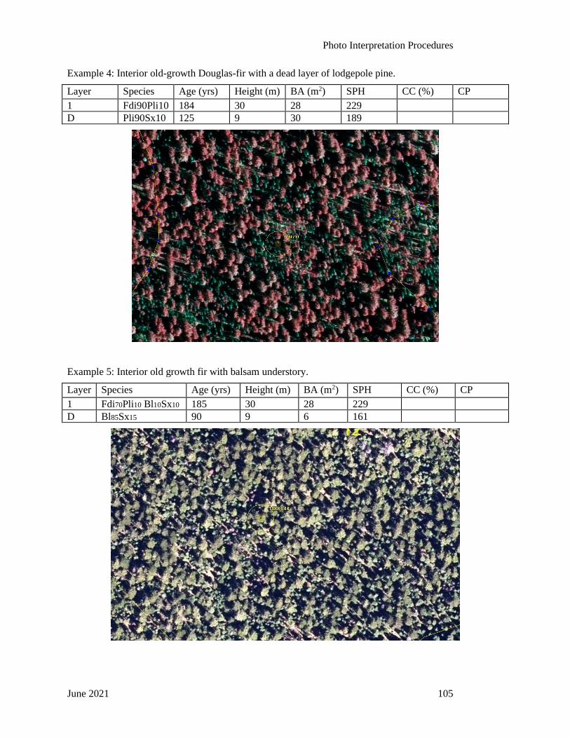
Photo Interpretation Procedures
June 2021 105
Example 4: Interior old-growth Douglas-fir with a dead layer of lodgepole pine.
Layer Species Age (yrs) Height (m) BA (m2) SPH CC (%) CP
1 Fdi90Pli10 184 30 28 229
D Pli90Sx10 125 9 30 189
Example 5: Interior old growth fir with balsam understory.
Layer Species Age (yrs) Height (m) BA (m2) SPH CC (%) CP
1 Fdi70Pli10 Bl10Sx10 185 30 28 229
D Bl85Sx15 90 9 6 161
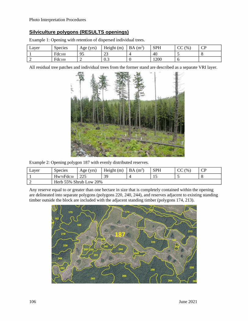
Photo Interpretation Procedures
106 June 2021
Silviculture polygons (RESULTS openings)
Example 1: Opening with retention of dispersed individual trees.
Layer Species Age (yrs) Height (m) BA (m2) SPH CC (%) CP
1 Fdc100 95 23 4 40 5 8
2 Fdc100 2 0.3 0 1200 6
All residual tree patches and individual trees from the former stand are described as a separate VRI layer.
Example 2: Opening polygon 187 with evenly distributed reserves.
Layer Species Age (yrs) Height (m) BA (m2) SPH CC (%) CP
1 Hw70Fdc30 225 39 4 15 5 8
2 Herb 55% Shrub Low 20%
Any reserve equal to or greater than one hectare in size that is completely contained within the opening
are delineated into separate polygons (polygons 220, 240, 244), and reserves adjacent to existing standing
timber outside the block are included with the adjacent standing timber (polygons 174, 213).

Photo Interpretation Procedures
June 2021 107
Example 3: Opening polygon 220 with unevenly distributed reserves each reserve below 1 ha.
Layer Species Age (yrs) Height (m) BA (m2) SPH CC (%) CP
1 Fdc100 55 33 4 35 5 3
2 Fdc90Dr10 8 3 0 435 10 8
Attribute as a two-layer stand with no further delineation.
Example 4: Opening polygon with two distinct layers and the same leading species.
Layer Species Age (yrs) Height (m) BA (m2) SPH CC (%) CP
1 Bl100 101 20 6 35 5 8
2 Bl100 35 7 1 1600 30 9

Photo Interpretation Procedures
108 June 2021
Appendix B Cover Patterns
1. Single to very few (<4) occurrences of limited extent, circular to
irregular shape.
2. Single to very few (<4) occurrences of limited extent, linear or
elongated shape.
3. Several (>3) sporadic occurrences of limited extent, circular to
irregular shape.
4. Several (>3) sporadic occurrences of limited extent, linear or
elongated shape.
5. Discontinuous but extensive occurrences, parallel to
sub-parallel, elongated in shape.
6. Intimately intermixed units, often with gradational transitions from
one to the other.
7. Limited continuous occurrence with few inclusions.
8. Continuous occurrence with several inclusions.
9. Continuous occurrence with very few inclusions.
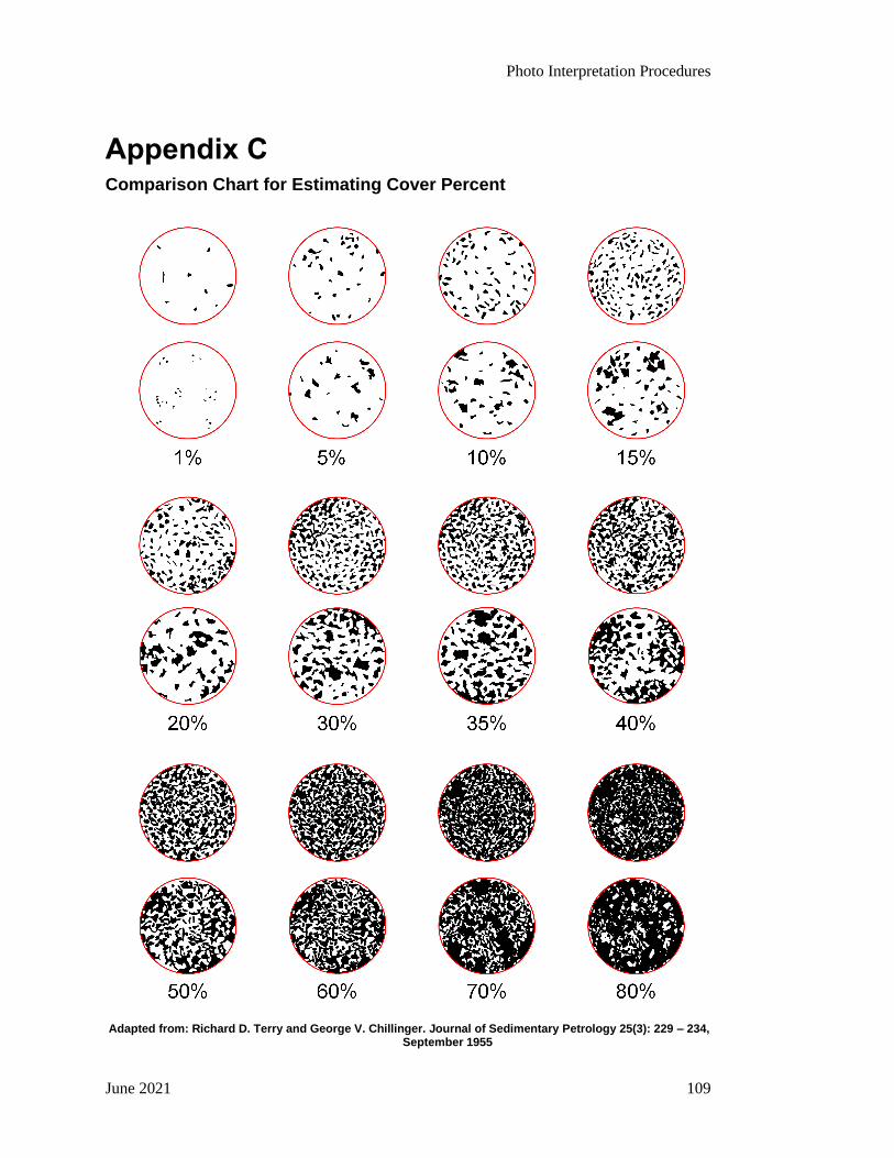
Photo Interpretation Procedures
June 2021 109
Appendix C Comparison Chart for Estimating Cover Percent
Adapted from: Richard D. Terry and George V. Chillinger. Journal of Sedimentary Petrology 25(3): 229 – 234,
September 1955

Photo Interpretation Procedures
110 June 2021
Appendix D Derived Polygon Attributes
1.0 Introduction
Photo interpreters delineate and assign many attributes to polygons on aerial imagery that describe the
land base and vegetation characteristics. A number of additional attributes can be derived, in a consistent
manner, from the estimated attributes. For example, the tree cover site index can be derived from the
estimates for species, age, and height. Similarly, the land cover class code can be derived from the
landscape position, vegetation type, and crown closure estimates.
This section presents a discussion of the additional attributes, referred to as "derived attributes,” that have
been identified as a product of the Photo Interpretation phase of the Vegetation Resources Inventory.
While the provision of these estimates is not the immediate task of the photo interpreter, it is important
that their derivations and the associations with the photo-interpreted attributes are understood.
In this respect, photo interpreters are encouraged to consider the extension of the Photo-interpreted
information being provided.
The following list presents the attributes identified for derivation from the photo-interpreted attributes that
may be subsequently adjusted with Ground Sampling data:
• Land cover class code
• Dominant polygon soil moisture regime (SMR)
• Tree diameter at breast height (DBH)
• Tree volume
• Tree site index
• Polygon descriptions for multi-layered stands
2.0 Land Cover Class Code
2.1 Definition
The land cover class code is the land cover designation of the polygon, consistent with the BC Land
Cover Classification Scheme.
2.2 Purpose
The land cover class code provides a categorization of the polygon to the most detailed land cover
description level of the BC Land Cover Classification Scheme. This information can be used for the
classification of individual polygons and can be summarized for national and international reporting.
2.3 Derivation Procedure
The BC Land Cover Classification Scheme's five levels are derived from the photo interpreter’s estimates
as follows. (See Section 2: BC Land Cover Classification Scheme for a detailed description of the levels.)

Photo Interpretation Procedures
June 2021 111
Vegetated
Level 1 Land base - Vegetated versus Non-Vegetated
Level 1 is derived from the sum of the vegetation crown closures.
Level 2 Land cover type (Treed versus Non-Treed)
Level 2 is derived from the tree crown closure estimate.
Level 3 Landscape Position (Wetland, Upland or Alpine)
The Alpine designation indicates polygons that fall in the alpine regions of the landscape. For
all other polygons, land cover component #1 soil moisture regime will determine whether that
polygon is considered to be Upland or Wetland. The BC Land Cover Classification Scheme
presents the designations "Wetland, Upland, and Alpine" as being mutually exclusive; however,
it is possible in some rare cases to have a wetland polygon in an alpine setting. The current
format of the scheme is maintained due to the infrequency of this occurrence.
Level 4 Vegetation Type
An iterative process following the rules of the BC Land Cover Classification Scheme is
followed using the hierarchy of the Scheme. When the polygon is Treed, the basal area of each
species (expressed as percent composition) is reviewed and amalgamated to determine which
vegetation type the polygon should be classified as. When the polygon is Non-Treed, the
hierarchy of the Scheme is implemented to determine which vegetation type should be derived.
Level 5 Density
Level 5 is derived from specific vegetation type crown closure (or cover percent for Herb and
Bryoid cover types).
Non - Vegetated
Level 1 Land base - Vegetated versus Non-Vegetated
Level 1 is derived from the sum of the vegetation crown closures.
Level 2 Land Cover Type
Level 2 is derived using the Level 5 information and working in reverse order. Each non-
vegetated category can be directly correlated with a specific land cover type.
Level 3 Landscape Position
The Alpine designation indicates polygons that fall in the alpine regions of the landscape. For
all other polygons, land cover component #1 soil moisture regime will determine whether that
polygon is considered to be Upland or Wetland. The BC Land Cover Classification Scheme
presents the designations "Wetland, Upland and Alpine" as being mutually exclusive; however,
it is possible in some rare cases to have a wetland polygon in an alpine setting. The current
format of the scheme is maintained due to the infrequency of this occurrence.
Level 4 Non-Vegetated Cover Type
Level 4 is derived using the level 5 information and working in reverse order. There is a direct
correlation between each Non-Vegetated category and a specific Non-Vegetated cover type. No
level 4 codes exist for water bodies; therefore, these fields are left blank for Water cover types.
Level 5 Non-Vegetated Categories
The codes from level 5 will be assigned directly by the photo interpreter as part of the attribute
estimation process.

Photo Interpretation Procedures
112 June 2021
Examples:
A typical derivation of a Vegetated Land Cover Class Code:
Level Estimated attribute criteria Code
1 Vegetated crown closure ≥ 5% V
2 Tree crown closure ≥ 5% T
3 Not Alpine and LCC #1 SMR = 4 U
4 Species composition = Pl80At20 TC
5 Tree crown closure = 80% DE
The Land Class Code for this polygon would be "VTUTCDE."
An example of a derivation of a Non-Vegetated Land Cover Class Code:
Level Estimated attribute criteria Code
1 Vegetated crown closure < 5% N
2 Level 5 = Rubble, Talus, Blockfield L
3 Alpine A
4 Level 5 = Rubble, Talus, Blockfield RO
5 Photo interpreted as Talus TA
The Land Class Code for this polygon would be "NLARORT."
3.0 Dominant Polygon Soil Moisture Regime
3.1 Definition
The dominant polygon soil moisture regime (SMR) is an estimate of the soil moisture for the polygon.
3.2 Purpose
Dominant polygon SMR provides soil moisture information at the polygon level, thus facilitating broad
reporting capabilities.
3.3 Derivation Procedure
Dominant polygon SMR is derived from the largest land cover component by area. When the first two or
more land cover components are equal in percent area, the first land cover component indicated will be
used to derive the dominant SMR.
4.0 Tree Diameter at Breast Height (DBH)

Photo Interpretation Procedures
June 2021 113
4.1 Definition
Diameter at breast height (DBH) is the average tree diameter at breast height for all live trees in the
dominant, co-dominant, and high intermediate crown positions in each tree layer in the polygon.
Note: Dominant trees have well-developed crowns that extend above the general level of the trees
around them. Co-dominant trees have crowns forming the general level of trees around them.
High intermediate trees have smaller crowns slightly below but extending into the general level of
trees around them.
4.2 Purpose
DBH provides an additional dimension of tree stand information that is useful for broad silviculture
planning (particularly for lower productivity, interior lodgepole pine stands), as well as change
management of some forest stands.
4.3 Derivation Procedure
DBH of the visible trees can be derived from the estimates provided for basal area per hectare and density
using the following method:
DBH = 2 * √Basal Area
(Density x π )
For example, if basal Area = 100 m2per ha and density = 400 stems per ha
DBH = 2 *14.3400
100 2
xhaperstems
haperm = 2 *
20796.0 m = 0.564 m
DBH = 56.4 cm
5.0 Tree Volume
5.1 Definition
Volume is the average gross stem volume of all living trees visible to the photo interpreter for the
polygon, expressed in cubic metres per hectare.
5.2 Purpose
The derivation of volume estimates for each polygon provides another method of assessing timber yields
and can be useful for long-term resource planning.
Derivation Procedure
5.3 Derivation Procedure
Volume can be derived from estimates provided for basal area, species composition, and height. Leading
species and the vegetation inventory project location (e.g., Forest Inventory Zone) determines which taper
equations and which decay, loss, and breakage factors are appropriate for volume derivation. Basal area
and height then provide the essential input parameters from which volume estimates can be derived.
A very simplified formula to calculate tree volume is:

Photo Interpretation Procedures
114 June 2021
Gross volume = 1/3 × height × basal area
For example, if basal area = 57 m2 per ha and height = 42 m
Gross volume = 1/3 × 42 m × 57 m2 per ha
Gross volume = 798 m3 per ha
This is a simplified approach for demonstration purposes only. The actual process and formula used to
derive the volume that will be stored in the database will incorporate many more factors than the formula
indicated above.
6.0 Tree Site Index
6.1 Definition
Site index is an estimate of site productivity for tree growth, expressed as a height (in metres) at breast
height age of 50 years for a particular tree species.
6.2 Purpose
Site index provides an estimate of the site productivity for tree species growth.
6.3 Derivation Procedure
Site index estimates are required on all treed polygons as well as polygons that are potentially capable of
producing trees. Stands that are 30 years or older will have the site index derived from species, age, and
height. The photo interpreter can still override the process if they:
• Have field data to provide site-specific values
• Have evidence to indicate abnormal site suppression exists
Leading species indicates which species height/age curves should be used. Age and height estimates then
indicate which of the available curves should be used for extrapolation (age less than 50 years) or
interpolation (age greater than 50 years) of site index.
7.0 Polygon Description for Multi-layered Stands
7.1 Definition
The polygon description for multi-layered stands is a summary of the attribute estimates for each
observable tree layer into one set of attribute estimates for the polygon.
7.2 Purpose
Ground sampling data does not differentiate trees from different layers within a stand. Therefore,
attributes from individual tree layers need to be amalgamated into a single polygon description to
facilitate inventory adjustments.
The adjustment is followed by a redistribution of the adjusted attribute values into the original individual
tree layer estimates.
7.3 Derivation Procedure
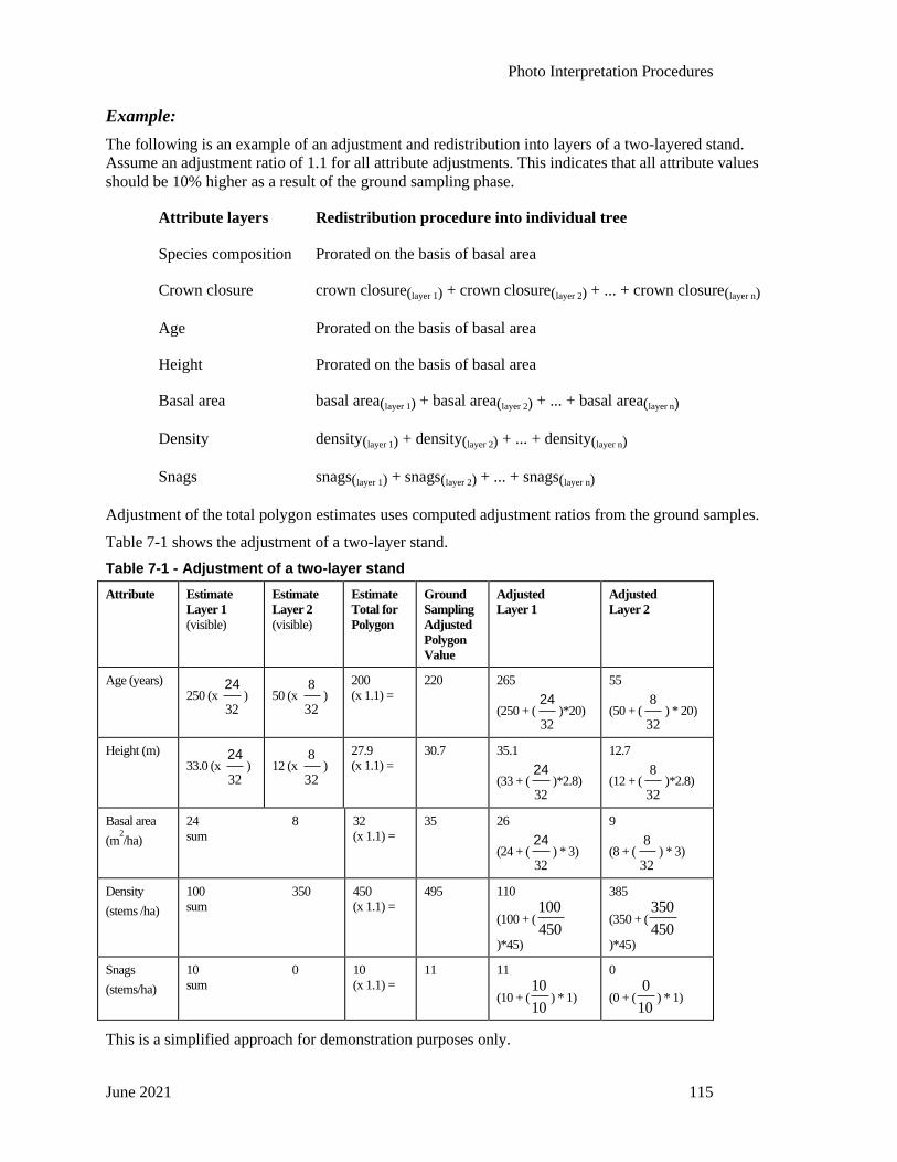
Photo Interpretation Procedures
June 2021 115
Example:
The following is an example of an adjustment and redistribution into layers of a two-layered stand.
Assume an adjustment ratio of 1.1 for all attribute adjustments. This indicates that all attribute values
should be 10% higher as a result of the ground sampling phase.
Attribute layers Redistribution procedure into individual tree
Species composition Prorated on the basis of basal area
Crown closure crown closure(layer 1) + crown closure(layer 2) + ... + crown closure(layer n)
Age Prorated on the basis of basal area
Height Prorated on the basis of basal area
Basal area basal area(layer 1) + basal area(layer 2) + ... + basal area(layer n)
Density density(layer 1) + density(layer 2) + ... + density(layer n)
Snags snags(layer 1) + snags(layer 2) + ... + snags(layer n)
Adjustment of the total polygon estimates uses computed adjustment ratios from the ground samples.
Table 7-1 shows the adjustment of a two-layer stand.
Table 7-1 - Adjustment of a two-layer stand
Attribute Estimate
Layer 1
(visible)
Estimate
Layer 2
(visible)
Estimate
Total for
Polygon
Ground
Sampling
Adjusted
Polygon
Value
Adjusted
Layer 1
Adjusted
Layer 2
Age (years)
250 (x 32
24) 50 (x
32
8)
200
(x 1.1) =
220 265
(250 + (32
24)*20)
55
(50 + (32
8) * 20)
Height (m)
33.0 (x 32
24) 12 (x
32
8)
27.9
(x 1.1) =
30.7 35.1
(33 + (32
24)*2.8)
12.7
(12 + (32
8)*2.8)
Basal area
(m2/ha)
24 8
sum
32
(x 1.1) =
35 26
(24 + (32
24) * 3)
9
(8 + (32
8) * 3)
Density
(stems /ha)
100 350
sum
450
(x 1.1) =
495 110
(100 + (100
450)*45)
385
(350 + (350
450)*45)
Snags
(stems/ha)
10 0
sum
10
(x 1.1) =
11 11
(10 + (10
10) * 1)
0
(0 + (0
10) * 1)
This is a simplified approach for demonstration purposes only.