SANDIA REPORTSAND96-2775 • UC-706Unlimited ReleasePrinted February 1998

VECTORSA Fortran 90 Module for 3-DimensionalVector and Dyadic Arithmetic

Billy C. Brock

Prepared by

Sandia National Laboratories

Albuquerque, New Mexico 87185 and Livermore, California 94550

Sandia is a muitiprogram laboratory operated by Sandia Corporation,

a Lockheed Martin Company, for the United States Department of

Energy under Contract DE-AC04-94AL85000.

Approved for public release; further dissemination unlimited.

“(i5!i)Sandia National laboratories

<-r- L,,, q .,q -~.L.. c.

Issued by San&a National Laboratories, operated for the United StatesDepartment of Energy by Sandia Corporation.NOTICE: This report was prepared as an account of work sponsored by anagency of the United States Government. Neither the United States Govern-ment nor any agency thereof, nor any of their employees, nor any of theircontractors, subcontractors, or their employees, makes any warranty,express or implied, or assumes any legal liability or responsibility for theaccuracy, completeness, or usefulness of any information, apparatus, prod-uct, or process disclosed, or represents that its use would not in fi-inge pri-vately owned rights. Reference herein to any specific commercial product,process, or service by trade name, trademark, manufacturer, or otherwise,does not necessarily constitute or imply its endorsement, recommendation,or favoring by the United States Government, any agency thereof, or any oftheir contractors or subcontractors. The views and opinions expressedherein do not necessarily state or reflect those of the United States Govern-ment, any agency thereof, or any of their contractors.

Printed in the United States of America. This report has been reproduceddirectly from the best available copy.

Available to DOE and DOE contractors fromOffice of Scientific and Technical InformationP.O. Box 62Oak Ridge, TN 37831

Prices available from (615) 576-8401, FTS 626-8401

Available to the public fromNational Technical Information ServiceU.S. Department of Commerce5285 port Royal RdSpringfield, VA 22161

NTIS price codesPrinted copy: A03Microfiche copy: AO1

SAND96-2775Unlimited Release

Printed February 1998

DistributionCategory UC-706

VECTORSA Fortran 90 Module for 3-Dimensional Vector and

Dyadic Arithmetic

Billy C. BrockRadar/Antenna Department

Sandia National LaboratoriesAlbuquerque, New Mexico 87185-0533

Abstract

A major advance contained in the new Fortran 90 language standard is theability to define new data types and the operators associated with them.Writing computer code to implement computations with real and complexthree-dimensional vectors and dyadics is greatly simplified if the equations canbe implemented directly, without the need to code the vector arithmeticexplicitly. The Fortran 90 module described here defines new data types forreal and complex 3-dimensional vectors and dyadics, along with the commonoperations needed to work with these objects. Routines to allow convenientinitialization and output of the new types are also included. In keeping withthe philosophy of data abstraction, the details of the implementation of the datatypes are maintained private, and the functions and operators are made genericto simplify the combining of real, complex, single- and double-precisionvectors and dyadics.

3

This Page Intentionally Blank

Introduction ................................................................................................................................7

Overview of the Vector and Dyadic-Tensor Arithmetic Module ............................................... 8Data ~pes ...............................................................................................................................8Operators ................................................................................................................................ 8

Fuctions ................................................................................................................................9Subroutines .............................................................................................................................9

Description of the Vector and Dyadic Operators and Procedures .............................................. 9

Operators ................................................................................................................................ 9Assignment (=) ...................................................................................................................9Multiplication and Dot Products (*) ................................................................................. 10Cross Products (.X.) .................i....................................................................................... 10Scalar Division (~ ............................................................................................................. 10Addition (+) ...................................................................................................................... 11Subtraction and Negation(-) ............................................................................................. 11Negation (neg.) ................................................................................................................ 11

Dyadic Product (.dyad.) .................................................................................................... 11Functions .............................................................................................................................. 11

vector(x. y. z) .................................................................................................................... 11

dyadic(X, Y, Z) ................................................................................................................. 12

abso .................................................................................................................................- 12red() .................................................................................................................................. 12aimag~ .............................................................................................................................. 12conjg() ............................................................................................................................... 12unit_vectoro ..................................................................................................................... 12det() ................................................................................................................................... 13invo .................................................................................................................................. 13

trms~ ...............................................................................................................................- 13trace() ................................................................................................................................ 13get(A, i) ............................................................................................................................. 13eigen.values(A) ................................................................................................................ 13eigen_vector(B) ................................................................................................................ 14

Subroutines ........................................................................................................................... 14

set(A.b.i) ........................................................................................................................... 14write([lun,] string, [edt,] A) ............................................................................................... 15

Summary of Vector and Dyadic &ithetic ............................................................................. 15Vectors .................................................................................................................................. 16

Dot Product Between Two Vectors .................................................................................. 16Cross Product Between Two Vectors ............................................................................... 17Associativity of Vector Dot and Cross Products .............................................................. 17

5

Dyads and Dyadics ............................................................................................................... 17Transpose of Dyadic ......................................................................................................... 18Trace of Dyadic ................................................................................................................ 18Vector Dot Product ........................................................................................................... 18

Cross Product Between a Dyadic and a Vector ................................................................ 19Associativity of Products of aDyadic and a Vector .........................................................2ODyadic Dot Product ..........................................................................................................2O

Eigen Values and Eigen Vectors .......................................................................................... 21

Appendix A: Solution of Cubic and Quartic Equations with Complex Coefficients ..............25Cubic Equation .....................................................................................................................25Qu~ic Equation ...................................................................................................................28References ............................................................................................................................3O

6

Introduction

A major advance contained in the new Fortran 90 language standard is the ability to definenew data types and the operators associated with them. Writing computer code to implementcomputations with real and complex 3-dimensional vectors and dyadics is greatly simplified ifthe equations can be implemented directly. In the past, it has been necessary to break theseinto separate equations for each of the individual components in order to code the vectorarithmetic explicitly. The Fortran 90 module described here defines new data types for realand complex 3-dimensional vectors and dyadics, along with the common operations needed towork with these objects. Routines to allow convenient initialization and output of the new

types are also included. In keeping with the philosophy of data abstraction, the details of theimplementation of the data types are maintained private, and the fhnctions and operators aremade generic to simpli~ the combining of real, complex, single- and double-precision vectorsand dyadics.

Module vectors has been used successfidly over the past year to simplifi and accelerate thedevelopment and maintenance of vector-intensive computational codes. Because these datatypes and associated operators are becoming embedded in numerous computer codes, some ofwhich may have an extended lifetime, it has become necessary to document the module. Bypublishing this documentation, I am not claiming that the implementation of this module is byany means optimal, but continued use of the module without appropriate documentation willcertainly be suboptimal. Other methods of implementation are certainly possible and valid. Ihave made choices in the design of this module that suited my personal programming taste,which continues to evolve.

In order to handle the many possible combinations of real, complex, single precision, double

precision, scalar, vector, and dyadic operands, the module has grown to a rather large size.The large size of the source code is a result of the necessity to include separate versions ofeach routine to handle the many different combinations of arguments. For example, a functionprocedure is included which takes three scalar arguments x, y, and z, and returns a vector oftype ( rea l_ve ct or ) with components x, y, and z along the principal axes. Thisfunction is necessary, because the default constructor is not available outside the module sincethe internal details of the new types are private. Naturally, a version exists where x, y, and zare all real, but in addition, versions exist where x is real but y and z are integers, and wherey is real but x and z are integers, and so on. Also similar functions exist for double precision,

complex, and double-precision complex vectors. All of these routines are mapped to onegeneric fimction vect or (x, y, z ) . With all of the possible combinations of arguments,there are 125 functions which are mapped to the same generic fimction, vect or (x, y,

z ) . All of these routines are essentially identical, except for type statements for thearguments and return variable, which must change from routine to routine. The necessity ofexplicitly defining routines for each case, rather than defining a template fimction as in C+,causes the source code to become very large. However, once the routines are written andtested, the module greatly simplifies the writing and maintenance of any programs which usevector and dyadic arithmetic.

Rather than include a listing of the source code, the source code is contained on the enclosed

high density 3.5” diskette in the MS-DOS format. The source code, vect ors. f 90, consists

of two modules, Vectors, and Roots, which is a module required by Vectors. This

source code has been compiled successfidly on an Intel Pentium-based computer with theLahey Fortran 90 compiler, version 2.Oli, with Microsoft PowerStation, version 4.0, and withDigital Visual Fortran, version 5.0. It has also been successfully compiled on a Sun Spare 20system with SunSoft Fortran 90, version 1.1. Although the code has been extensively usedand tested, it is not practical to test all possible circumstances, and no guarantee of accuracy orcorrectness of the code can be offered.

Overview of the Vector and Dyadic-Tensor Arithmetic Module

The Fortran 90 module Vectors contains type definitions and operators to facilitate three-

dimensional vector and dyadic-tensor arithmetic. The module (version 1.00) consists of 561function and 84 subroutine procedures. However, these procedures are maintained private,and are available to the user only through eight generic operators, fourteen generic functions,

and two generic subroutines.

Data typesThe module implements real and complex vectors in both single- and double-precisionnumerical kinds. The following eight new types are defined:

type (real_vector) -- single-precision real vector,

type (complex_vector) -- single-precision complex vector,

type (dbl_real_vector) -- double-precision real vector,

type (dbl_complex_vector) -- double-precision complex vector,

type ( real_dyadic ) -- single-precision real dyadic tensor,type (complex_dyadic) -- single-precision complex dyadic tensor,type (dbl_real_dyadic) -- double-precision real dyadic tensor,

type (dbl_complex_dyadic) -- double-precision complex dyadic tensor.

OperatorsAll procedures and operators are generic, accept any of the newly defined types, and return theappropriate result. The following generic operators are defined or extended to accept vectorand dyadic operands, as appropriate:

= assignment operator,* multiply vector or dyadic by scalar,

dot product between two vectors,dot product between a vector and a dyadic,dot product between two dyadics,

.x. cross product between two vectors,cross product between a vector and a dyadic,

/ divide a vector or a dyadic by a scalar,+ add two vectors or two dyadics,

subtract two vectors or two dyadics,negation of vector or dyadic

. neg. negation of vector or dyadic,

8

.dyad. dyadic vector product (product of two vectors without dot or crosssymbol, resulting in a dyad).

Operator precedence for the extended operators is the same as for the original Fortran 90operators, while the new operators (. x.,.ne g., . dyad. ) have the lowest precedence.

FunctionsThe following generic fimctions are supported:

vector (x, y, z) creates a vector from three scalar components,

dyadic (X, Y, Z) creates a dyadic from three vector components (the vectors X, Y, Z

are the left-hand factors of the dyads and form the columns whenthe dyadic is represented as a matrix; the dyadic created is

fi+l?j+fi),

abs ( ) returns the magnitude of a vector,

real ( ) returns the real part of a complex vector or dyadic,

aimag ( ) returns the imaginary part of a complex vector or dyadic,

conj g ( ) returns the complex conjugate of a complex vector or dyadic,

unit_vector ( ) creates a unit vector in the direction of the vector argument,

det ( ) returns the determinant of a dyadic,

inv ( ) returns the inverse of a dyadic,

trans ( ) returns the transpose a dyadic,

trace ( ) computes the trace of a dyadic (sum of diagonal elements)

get (A, i) returns the ith Cartesian element (i=l ,2,3) of a vector or a dyadic(returns a scalar when A is a vector and a vector when A is adyadic),

e i gen_va 1 ues (A) returns an array of 3 complex eigen values of the dyadic A,

eigen_vect or (B ) returns the eigen vector, 6, of dyadic B,such that B” $ = O.

SubroutinesThe following subroutines are included:

set(A, b, i.) sets element i of A to value of b, where b is a scalar when A is avector and a vector when A is a dyadic,

write ( [lun, ] string, [edt, ] A)writes a string followed by a vector or dyadic, A, to the defaultoutput device, or to the optional logical device (1 un, an integer).The optional edit descriptor (edt) is any valid edit descriptorstring for a Fortran 90 real type, for example ‘f6.2’.

Description of the Vector and Dyadic Operators and Procedures

Operators

Assignment (=)The assignment operator expects to find the name of a vector or dyadic on the left side,and a vector or dyadic expression on the right. The left-side variable is assigned the

9

value of the right-side expression. Type conversion between vector types or betweendyadic types is performed. However, the left and right operands must be either bothvectors or dyadics. When the right side is a complex or double-precision complex

vector or dyadic expression, and the left-hand variable is real or double precision, it isassigned the value of the real part of the right-hand side; the imaginary part is simply

lost. The complete functionality is implemented with 24 private subroutine proceduresinterfaced to the assignment operator, =.

Multiplication and Dot Products (*)The multiplication and dot product operator can return a dyadic, vector, or scalarresult, depending on the types of the operands. A vector or dyadic can be multipliedby a scalar, two vectors can be dot multiplied, a vector and a dyadic can be dotmultiplied, and two dyadics can be dot multiplied.

Scalar multiplication allows the scalar (which can be of any numerical type, includinginteger) to be on the left or the right side of the operator. The other operand can be any

of the four vector types or four dyadic types. The result will be a vector or a dyadic, asappropriate, of the highest numerical kind contained in the operands. For example,multiplying a real vector by a complex scalar will return a complex vector.

When neither operand is a scalar, the operator implements the dot product between the

operands. The dot product of two vectors returns a scalar of the highest numericalkind contained in the operands. The dot product between a vector (on the left or theright) and a dyadic is a vector. A dot product between two dyadics returns a dyadic ofthe highest numerical kind contained in the operands. The meaning of vector anddyadic dot products is described in the Summary of Vector and Dyadic Arithmetic,

below.

The complete fimctionality requires 144 private fimction procedures interfaced to themultiplication and dot product operator, *.

Cross Products (.X. )The cross-product operator, . X.,returns either a vector or a dyadic, depending on the

operands. If both operands are vectors, the result is a vector of the highest numericalkind contained in the operands. A cross product between a vector and a dyadic (withthe dyadic on either the left or the right side) produces a dyadic of the highestnumerical kind of the operands. The meaning of the cross product between a dyadicand a vector is discussed in the Summary of Vector and Dyadic Arithmetic, below.The cross product between two dyadics is not allowed, as it results in a tensor of rank3, and this type is not implemented in the module. The complete functionality of thecross-product operator, . X. requires an interface to 48 private fiction procedures.

Scalar Division (/)Scalar division is the only division operator defined. A vector or a dyadic can bedivided by a scalar of any numerical kind. The scalar must be on the right. If a vectoror dyadic appears immediately to the right of the division operator, an error occurssince no operation is defined for this case. The result of the scalar division is a vector

10

or dyadic, as appropriate, of the highest numerical kind appearing in the operands.The complete functionality requires interfacing the division operator, /, to 40 privatefunction procedures.

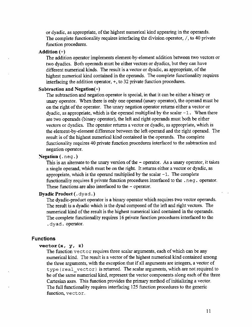
Addition (+)The addition operator implements element-by-element addition between two vectors ortwo dyadics. Both operands must be either vectors or dyadics, but they can havedifferent numerical kinds. The result is a vector or dyadic, as appropriate, of thehighest numerical kind contained in the operands. The complete fi.mctionality requiresinterfacing the addition operator, +, to 32 private fiction procedures.

Subtraction and Negation(-)The subtraction and negation operator is special, in that it can be either a binary orunary operator. When there is only one operand (unary operator), the operand must beon the right of the operator. The unary negation operator returns either a vector ordyadic, as appropriate, which is the operand multiplied by the scalar -1. When there

are two operands (binary operator), the left and right operands must both be eithervectors or dyadics. The operator returns a vector or dyadic, as appropriate, which isthe element-by-element difference between the left operand and the right operand. Theresult is of the highest numerical kind contained in the operands. The completefunctionality requires 40 private fimction procedures interfaced to the subtraction andnegation operator.

Negation (. neg. )This is an alternate to the unary version of the - operator. As a unary operator, it takesa single operand, which must be on the right. It returns either a vector or dyadic, asappropriate, which is the operand multiplied by the scalar – 1. The completefunctionality requires 8 private function procedures interfaced to the . ne g. operator,These fbnctions are also interfaced to the - operator.

Dyadic Product (. dyad. )The dyadic-product operator is a binary operator which requires two vector operands.The result is a dyadic which is the dyad composed of the lefi and right vectors. Thenumerical kind of the result is the highest numerical kind contained in the operands.The complete fimctionality requires 16 private fi.mction procedures interfaced to the. d yad. operator.

Functions

vector (x, y, z)The function vector requires three scalar arguments, each of which can be anynumerical kind. The result is a vector of the highest numerical kind contained amongthe three arguments, with the exception that if all arguments are integers, a vector oftype (rea l_vect or ) is returned. The scalar arguments, which are not required tobe of the same numerical kind, represent the vector components along each of the threeCartesian axes. This function provides the primary method of initializing a vector.The fill fimctionality requires interfacing 125 Iinction procedures to the generici%.nction, ve ct or.

11

dyadic(X, Y, Z)The function dyadi. c requires three vector arguments, and returns a dyadic of thehighest numerical kind contained in the three arguments. The arguments must bevectors, but are not required to be of the same numerical kind. The vectors X, Y, Z are

the left-hand factors of the dyads and form the columns when the dyadic is represented

as a matrix. The dyadic created is R + ~j + ~ii, where i, ~, and 2 are unit vectors

along the Cartesian axes. This fhnction provides the primary method of initializing adyadic. The till functionality requires interfacing of 64 private function procedures tothe generic fimction, dyadic.

absoThis fi.mction extends the intrinsic fi.mction of the same name, and returns themagnitude of a vector argument. The argument can be any of the four kinds of vector,and the numerical kind of the result is single or double precision, depending on thenumerical kind of the argument. The result is real and always greater than or equal tozero. The till fi.mctionality requires interfacing 4 private function procedures to thegeneric fimction, abs.

real ( )This fimction extends the intrinsic function of the same name, and returns the real partof a complex vector or dyadic argument. The argument can be eithertype (complex vector), type (dbl complex vector,type (complex~dyadic), or t ype (d~l_compl=x_dy adi-c), and thenumerical kind of the result is single or double precision, depending on the numericalkind of the argument. The full functionality requires interfacing 4 private fimctionprocedures to the generic fimction, rea 1.

aixnag ( )This fimction extends the intrinsic function of the same name, and returns theimaginary part of a complex vector or dyadic argument. The argument can be eithertype (complex_vector), type (dbl_complex_vector,type (complex_dyadic), or t ype (dbl_complex_dy adic ), and thenumerical kind of the result is single or double precision, depending on the numericalkind of the argument. The full functionality requires interfacing 4 private functionprocedures to the generic fi.mction, a imag.

conjg ( )This function extends the intrinsic function of the same name, and returns the complexconjugate of a complex vector or dyadic argument. The argument can be either

type (complex_vector ), type (dbl_complex_vector,type (complex_dyadic ), or t ype (dbl_complex_dyadic ), and the type ofthe result will match the type of the argument. The fill fimctionality requiresinterfacing 4 private function procedures to the generic function, con j g.

unit vector ( )~vs fhnction accepts a vector argument of any of the four kinds of vectors, and returnsa unit vector in the same direction. The unit vector is obtained by dividing theargument by its absolute value (magnitude). The result is a vector of the same type asthe argument, and is real if the argument is a real vector and complex if the argument

12

is a complex vector. The full functionality is obtained with 4 private fimctionprocedures interfaced to the generic function, unit_vect or.

det ( )This function accepts a dyadic argument, which can be any one of the four kinds ofdyadics, and returns the scalar value of the determinant of the argument. The result issingle or double precision, depending on the numerical kind of the argument, and willbe complex when the dyadic is a complex dyadic. The full fimctionality is obtainedwith 4 private function procedures interfaced to the generic fiction de t.

inv ( )This function accepts a dyadic argument, which can be any one of the four kinds ofdyadics, and returns the inverse dyadic, which, when dot multiplied with the argument,

will result in the unit dyadic. The result will have the same type as the argument. Thefull functionality is obtained with 4 private fimction procedures interfaced to thegeneric fimction inv.

trans ( )This fhnction accepts a dyadic argument, which can be any one of the four kinds ofdyadics, and returns the transpose of the dyadic. The result will have the same type as

the argument dyadic. The fill functionality is obtained with 4 private fimctionprocedures interfaced to the generic function trans.

trace ()This function accepts a dyadic argument, which can be any one of the four kinds ofdyadics, and returns the scalar value of the trace (sum of diagonal elements) of thedyadic. The result will have the same numerical kind as the argument dyadic. The fullfimctionality is obtained with 4 private function procedures interfaced to the genericfunction trace.

get(A, i)This fi.mction accepts two arguments. The first is a vector or dyadic, which can be any

one of the four kinds of vectors or dyadics, and the second is an integer between 1 and3. The integer indicates which Cartesian component to return. When the first

argument is a vector, the fiction returns the scalar which is the ifh Cartesiancomponent. When the first argument is a dyadic, the function returns the vector which

is the i’~ Cartesian vector component when the dyadic is written with the Cartesian

unit vectors on the right side. This is the i’h column when the dyadic is written as a

matrix. The value (scalar or vector) returned by get is identical to the value obtained

by taking the dot product of the argument with the i’h unit vector on the right side.

For example, get (A, 2 ) returns the scalar ~. ~ when A is a vector, and returns the

vector ~” ~ when A is a dyadic. The numerical kind of the result matches that of the

argument. The fill functionality is obtained with 8 private fimction proceduresinterfaced to get.

13

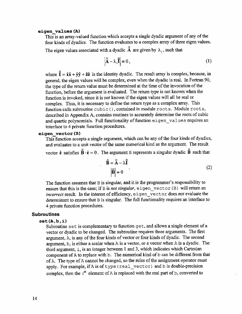
eigen values(A)Tl&is an array-valued function which accepts a single dyadic argument of any of thefour kinds of dyadics. The fi.mction evaluates to a complex array of three eigen values.

The eigen values associated with a dyadic ~ are given by Li, such that

(1)

where ~ = ii + ~ + % is the identity dyadic. The result array is complex, because, in

general, the eigen values will be complex, even when the dyadic is real. In Fortran 90,

the type of the return value must be determined at the time of the invocation of thefunction, before the argument is evaluated. The return type is not known when thefunction is invoked, since it is not known if the eigen values will all be real orcomplex. Thus, it is necessay to define the return type as a complex array. Thisfimction calls subroutine cubic (), contained in module roots. Module roots,described in Appendix A, contains routines to accurately determine the roots of cubicand quartic polynomials. Full fimctionality of function e i gen va 1 ues requires an—interface to 4 private fimction procedures.

eigen_vector (B)This fimction accepts a single argument, which can be any of the four kinds of dyadics,

and evaluates to a unit vector of the same numerical kind as the argument. The result

vector 6 satisfies B 06 = O. The argument B represents a singular dyadic B such that

B=i–?biB=o “

(2)

The function assumes that B issingular, and it is the programmer’s responsibility toensure that this is the case; if B isnotsingular, e i gen_ve ct or (B) will return anincorrect result. In the interest of efficiency, e igen_ve ct or does not evaluate thedeterminant to ensure that B issingular. The fill fimctionality requires an interface to4 private fiction procedures.

Subroutines

set(A, b,i)Subroutine set is complementary to function get, and allows a single element of avector or dyadic to be changed. The subroutine requires three arguments. The firstargument, A,is any of the four kinds of vector or four kinds of dyadic. The secondargument, b, is either a scalar when A isa vector, or a vector when A is a dyadic. Thethird argument, i, is an integer between 1 and 3, which indicates which Cartesiancomponent of A to replace with b. The numerical kind of b can be different from thatof A. Thetype of A cannot be changed, so the rules of the assignment operator mustapply. For example, if A isoft ype ( rea 1 vector) and b is double-precision—complex, then the i’h element of A isreplaced with the real part of b, converted to

14

single precision. The imaginary part is lost since A is a real type. Full fi.mctionality

requires 28 private subroutine procedures interfaced to the generic subroutine set.

write ( [lun, ] string, [edt, ] A)Subroutine writ e is the only output routine supplied by the module. It will accept up

to four arguments; the arguments enclosed between [ ] are optional. If the firstargument is an integer, then it refers to the logical unit to which the output is to bewritten. In this case, the logical unit must have been opened previously. If thisargument is omitted, then the output is written to the standard output device (usuallythe terminal). The second argument is required, and is a string used to label the output.The string can have any length, and can even bean empty string, ‘ ‘. The thirdargument is optional, and must be a valid Fortran 90 edit descriptor for a real number(forexample, ‘f10.4’, ‘lpg15.7’, ‘ lpe23. 15’, etc.). If this argument is

omitted, then the output is written using gl 3.7 for single precision quantities andg21. 15 for double precision quantities. The last argument, A, is required and is thequantity to be written. It can be any of the four kinds of vector or any of the four kindsof dyadic. The subroutine formats A into a form which is easy to read. For example,the code fragment

use Vectorstype (real_vector) :: u, vtype (real_dyadic) :: Au = vector( 1.0, 2.0, 3.0 )v = vector ( -3.0, 2.0, 1.0 )call write (‘vector u = ‘, u)call write (‘vector u = ‘, ‘f5.2’, u)A = dyadic (u, v .X. u, v)call write (‘dyadic A = ‘, A)call write (’dyadic A = ‘, ‘f6.2’, A)

will produce the following output on the default display:vector u = [ 1.000000

2.0000003.000000 1

vector u = [ 1.002.003.00 ]

dyadic A = [ 1.000000 4.0000002.000000 10.000003.000000 -8.000000

dyadic A = [ 1.00 4.00 -3.002.00 10.00 2.003.00 -8.00 1.00 ]

-3.0000002.0000001.000000 1

15

Summary of Vector and Dyadic Arithmetic

VectorsThe Cartesian coordinate system illustrated in Fig. 1 will be used to describe the vectors anddyadic tensors (usually referred to simply as dyadics). A vector ii is defined, as illustrated, byits components along each coordinate axis

ii=ax%i -ayf+azii. (3)

Dot Product Between Two Vectors

The dot product defined between two vectors, 5 and h, is called the scalar dot product, andyields a scalar given by

ii. k = axbx + ayby +azbz. (4)

It can be seen that the scalar dot product is commutative; that is, the commutator is zero

ii” b- b”ii=o. (5)

\\

\

~\

\

Fig. 1 Reference coordinate system used to describe the vectors and dyadics.

16

Cross Product Between Two VectorsThe cross product defined between two vectors satisfies the following conditions for theCartesian unit vectors

ixk=fxf=%xk=o,

ix f=–fxk=i,

fxi=–ixy=i,

and

ixi=–ixi=f.

The cross product between two vectors is not commutative

iixii-Gxii *o,

but it is anticommutative (the anticommutator is zero)

iixb+bxz=o.

Associativity of Vector Dot and Cross Products

(6)

(7)

(8)

(9)

(lo)

(11)

Note that the sc&r dot product and the cross product between two vectors do not form an

associative pair of operators. The operations in the expression ii. ~ x E can only be performed

in one order because (5” ~) x ii has no meaning; the operator x requires two vector operands,

not a scalar and a vector operand. Because of the precedence rules in Fortran 90, the operatorrepresenting the cross product, . X., has a lower precedence than the operator representing the

dot product, *. Thus the expression ii”hx~ must be coded a* (b. X. c) ,because a*b. X. c

will cause an error. Since, in keeping with the precedence rules, a *b is evaluated first in theexpression a *b. X. c, the left operand for the .X. operator is of the wrong type (scalar, not ‘ -vector).

Dyads and DyadicsA dyad is the product of two vectors, written without any symbol separating them,

P=fi. (12)

A dyad has, at most, six independent scalar components. A dyadic tensor (often shortened todyadic) is a sum of dyads,

Q = Q=i% + QZY@+ Q=% .

+QFf~ + QW~ + QVW. (13)

+Q@i + QzY2j+ Q.fi

A dyadic has nine scalar components, or three vector components. The dyadic Q can be

written

17

Q=%~+qyf+wwhere the component vectors are

% = Q3 + QJ + Q.~

~Y= Qv~+ QJ + QJ “q, = Q=?+ QJ + Q,Zi

This is the particular decomposition of a dyadic into vector components that is implemented inthe module. An alternate decomposition can also be used

Q=@x+fPy+~Pz> (16)

where the component vectors are

p, = QU%+ QJ + QZZ2

Fy = Qpi + QJ + Qpi . (17)

F, = Qz~+ QJ + Q..%

For a nonsymmetric dyadic, iji # ~i, while for a symmetric dyadic, ~i = ~i. The function

dyadi. c (qx, w, qz ) uses the representationin(14) to create the dyadic 6 where qx I

qy, qz are the vectors definedby(15). Note that, if the ~i are known instead, Q can be

created with trans (dyadic (px, py, pz ) ) , where trans ( ) is the transposeoperation.

Transpose of DyadicThe transpose of a dyadic exchanges the order of the vectors in the dyads, so that

Trace of DyadicThe trace of a dyadic

trace(Q) = ~ Qii ,i=x,y,z

and the trace of a dyad Zk is the scalar dot product between the two vectors,

trace(iib) = ii” G.

(14)

(15)

(18)

(19)

(20)

18

Vector Dot Product

The vector dot product is the dot product between a dyadic, Q, and a vector, 5, and is the

vector given by

Q.ii=ax~x + ay~y + a:~z. (21)

Another vector dot product also exists

~”Q=Qx + aypy+ O,. (22)

From the definition of the transpose (1 8), it is seen that

(23)

The vector dot product is not commutative, unless the dyadic is symmetric. Thus, in general,the commutator for the vector dot product is not zero

~. Q–Q. ~#o, (24)

but, when Q is symmetric,

~“Q3ymmetric-Q symmetric“5 =0. (25)

Note that the vector dot product is similar to the multiplication of a square matrix by a columnor row matrix, except that the column matrix must be transposed to a row matrix when movedfrom the right side of the square matrix to the left side. Here, the similarity ends, because notranspose operation is needed for vectors in the vector-dyadic arithmetic. In fact, no transposeexists for these vectors. However, a transpose does exist for the dyadic.

Cross Product Between a Dyadic and a VectorA cross product between a vector and a dyadic is defined

Qx5=i(px xz)+y(py x5)+i(pz xii)

=qx(ix=)+qy(j x=)+qz(ixa) 7

( ) )=qya=– Gzay ~ + (~zax–oz)~ +(lay–~yax ~

(26)

when the vector is on the right or

when the vector is on the left. In general, the cross product between a vector and a dyadic is

not commutative

Qxa-5x Q#o. (28)

19

If the dyadic is symmetric, the cross product is anticommutative

Q ~metnc x ii + 5 x Q ~me,tic = 0, (29)

while if the dyadic is antisyrnmetric ( ~i = –jii ), the cross product is commutative

Q..@ymm.,r(.x g -5 x Qantjsynm.trj.= 0- (30)

Note that the diagonal elements, Qii, must be zero if the dyadic is antisymmetric.

Associativity of Products of a Dyadic and a VectorThe vector dot product and the cross product between a vector and a dyadic form anassociative pair of operators. Consider

(31)

In this case, the precedence rules do not interilere with the proper evaluation of the codea* Q.X.b,since either order will be valid and will give the same result. Similarly,

2ix(Q. G)=(5x Q).ii. (32)

Dyadic Dot ProductGiven two dyadics,

(33)

If the alternate representation of ~ is used,

20

c=ii5,+fGy+iez,then @e dot product is written simply

Q.s =(qxi+qyj+qz2) .(i6x +j%, +26=)

= qx~x +qy~y + %~z

Since

s.Q=(3xi+Fyj+szi).(qxi+qyj+q,i)

=Ex[(qx“ qi + (q, .i)j +(q, .+

+%[(%“w+(q,“J)t+-(q.“f)q ‘+3=[(%“q~ + (q “+ + (%“ +

we see that the commutator is not zero,

Q&& Q#o.

Eigen Values and Eigen Vectors

The eigen values associated with a dyadic ~ are given by Ii, such that

A–Lii=o,

(34)

(35)

(36)

(37)

where ~ = H + H + ti is the identity dyadic. The eigen vectors are the unit vectors, &i, such

that

(~-@”~i==”@ (38)

The eigen value equation leads to a cubic equation for the eigen values, Li. The solutions can

be real or complex. Note that if ~ is a real dyadic, then at least one of the eigen values is

real. However, since A is not constrained to be real, all of the Li may be complex. A

method of obtaining the roots of the cubic equation with complex coefficients is described inAppendix A, which documents the module roots.

Consider

B= bxi+byy+tzi,

for which

B=o.

(39)

(40)

The eigen-vector equation is

21

where

(41)

(42)

We can expand the determinant as follows

P.r,x PX,y Px,z

== Py,x Py,y Py,z

Pz,x Pz,y P.,,

= PXJPY,YPZ,Z- Py,zl%,y)- PX,Y(PY,XPZ,Z-PY,ZPZ,X)+PX,Z(PYAP2,Y-PY,YPZ,J

=BX”(BYXFZ)

= -Py,$x,y%,z - PX,ZPZ,Y)+ PY,Y(PX,XPZ,Z- PX,ZP,,X)- PY,Z(PXJPZ,Y- &,yPz,x) . (43)

=-~y .(FX x~z)

= PZ,X(PX,YPY,Z– PX,=PY,Y)- PJPX,XPY,. -PX,ZPY,X)+PZ,Z(PXJPY,Y-PX,YPY,J

=Fz “(BX@)

Since B = O, we see immediately that the eigen vector can be represented with either

a=pxx~y, (44)

or

t@xxpz, (45)

or

z=pyx~z. (46)

Also, since B = O, the three vectors B; contained in B are not independent. In fact, one of

the vectors, P,, must be a linear combination of the other two

pi= A~j +Bpk, (47)

22

where i,j, and k, represent any ordering of x, y, and z. Thus, we see that the three crossproducts are all parallel

and

(48)

(49)

Any of the three cross products can be used for the eigen vector, provided, of course, that A or

B is not zero. This amounts to saying that none of the ~i are parallel to each other. If a pair

of the ~ i happen to be parallel, then a cross product containing the other ~ i must be used. If

all three of the ~ i are parallel, then any vector perpendicular to ~ i can be used for the eigen

vector. Note that since the ~ i are dependent, they must all lie in the same plane. Thus, since

a plane has only one normal direction (to within a constant factor), all of the cross productsproduce the single unique solution to (41), to within a constant factor.

23

This Page Intentionally Blank

24

Appendix A: Solution of Cubic and Quartic Equations with ComplexCoefficients

Module roots contains procedures which solve for the roots of cubic and quartic equationswith complex coefficients. These routines are implemented only with double precision

arithmetic, in order to preserve the most precision in the roots. Subroutine cubic (a, b,c, z ) computes the three complex roots of

z3+az2+bz+c =0,

while subroutine qua rt i c (a, b, c, d, z ) computes the four complex roots of

z4+az3+bz2+cz+d =0.

The routines assume that the coefficients are complex, so the coefficients (a, b, c, d)must be defined as double-precision complex variables. Both subroutines return the roots in adouble-precision complex array, z, which must have at least 3 elements for a call to

cub i c ( ) and at least 4 elements for a call to quart i c ( ) . Note that subroutinequart i c ( ) is not used by module vectors. The methods implemented by the routinesare described below.

Cubic EquationThe solution of the cubic equation of the form

x3+ax2+bx+c=0 (A-1)

when the coefficients a, b, c are real numbers has been known since the 16th century. The

solution is attributed to Geronimo Cardano who published the solution in 1545. However, thesolution did not originate with Cardano. He obtained it from Niccolo Tartaglia in 1539, butthe solution is thought to have been first achieved by Scipione del Ferro around 1500.However, since Cardano was the first to publish it, the solution is known as Cardano’s formula[1]. The solution is published in many references [2,3,4, 5,6], but is valid as published onlyfor real coefficients. Here, the solution is simply extended to accommodate complexcoefficients. The extension is simple and straightforward.

The solution proceeds as follows. Let y = x – a / 3 so that

y3+py+q=o,

where

(A-2)

p= b–$,

and

ab 2a3

‘=c–y+ 27.

25

Now, let y = u+ v so that

u3+v3+(u +v)(p+3uv)+q=o. (A-3)

Since there are now two unknowns, a second constraint is needed. We are free to choose theconstraint in any way to expedite the solution, with the understanding that spurious roots mayarise. Cardano’s formula is based on the following constraints

u3+v3+q=o, (A-4)

and

(p+3uv)=o. (A-5)

Eliminating v results in

3

u6+qu3–~=o.27

(A-6)

Elimination of u results in the same equation with u replaced by v. Equation (A-6) is

quadratic in U3,and can be solved easily. Whenp is very small ( p - O), loss of precision in

the computation of one of the roots of a quadratic can occur, unless care is taken. In order topreserve the most precision in the roots, we use [7]

.s=-;[q+sw(q,~~)> (A-7)

U,= 3L~k; k= 0,1,2, (A-8)

and

~ E%;k=0J2whens#0‘k=[~~ ~9–sgn(9) q +4% <,; k= 0,1,2 when. = O

where. <k = eJk2*’3are the three cube roots of 1, and

I

1; Izl= o

Sgn(z) =~; lzl#o’

Z*

(A-9)

(A-1O)

where { represents the principal square root.

26

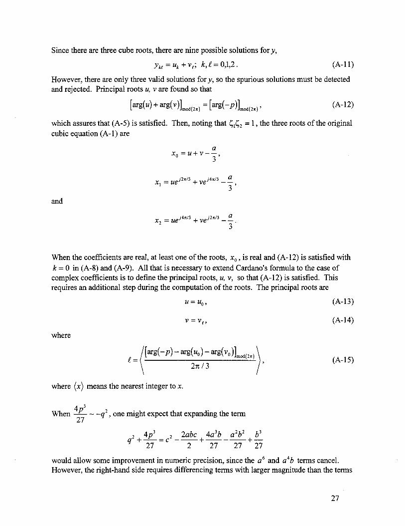
Since there are three cube roots, there are nine possible solutions for y,

)“k! = ‘k ‘Vt; ‘>~=0>1$2. (A-II)

However, there are only three valid solutions for y, so the spurious solutions must be detectedand rejected. Principal roots u, v are found so that

(A-12)

which assures that (A-5) is satisfied. Then, noting that <l~z = 1, the three roots of the original

cubic equation (A- 1) are

xo=u+v–~,3

x, = ue~zx’3+ veJ4’13– ~,3

and

X2 = ue-i4~13+ veJ2”i3 – ~.3

When the coefficients are real, at least one of the roots, XO,is real and (A-12) is satisfied with

k = O in (A-8) and (A-9). All that is necessary to extend Cardano’s formula to the case ofcomplex coefficients is to define the principal roots, u, v, so that (A-12) is satisfied. Thisrequires an additional step during the computation of the roots. The principal roots are

U=uo, (A-13)

‘=V[9 (A-14)

where

(~=[~g(-P)-~g(uo)- ~g(vo)lmd(2.)2n13

)

>

where (x) means the nearest integer to x.

When 4P3— - –q2, one might expect that expanding the term27

4p3 = ~2 2abc ~ 4a3b a=bz b3—— — ——‘2+ 27 2 27 27 ‘z

(A-15)

would allow some improvement in numeric precision, since the ab and a4b terms cancel.However, the right-hand side requires differencing terms with larger magnitude than the terms

27

on the left-hand side. Thus, precision will be lost if the expression on the right is used when

4p32. In this case, the simpler expression on the left is more accurate.

27 -‘q

Some increase in precision is obtained by refining the roots with one stage of Newton’smethod

c+xk,n(~+xk,n(~+xk,n))‘k,n+l = Xk,n –

b+ x,,n(2a +3xk,~) “(A-16)

Note that the polynomials are computed by factoring x from successive terms. This is done to

preserve numerical precision. Negligible improvement is obtained with a second stage ofrefinement.

Quartic EquationThe solution for the quartic equation,

x4+ax3+bx2+cx+d=o, (A-17)

was also obtained in the early part of the 16* century. It was found by L. Ferrari, a student of

Cardano, and subsequently published by Cardano [1]. The roots of (A-1 7) are

a R s(%)Xk=– —+a, —+ CZ2—

42 2’(A-18)

where

dR= $–b–y,

I~; ‘=0a,=il,

a2 =*1,

and y is any solution of the cubic equation [5]

y3–by2+ (ac–4d)y –a2d+4bd–c2 =0. (A-19)

Note that al and a2 are uncorrelated. Ths solution is valid when the coefficients me

complex.

28

Improved numerical precision is obtained with two stages of root refinement using Newton’smethod

d+ Xk,n(C + Xk,n(b+ Xky(a + Xk,n)))

‘k,n+l = Xk,n –c+ xk,n(2b +xk,n(3a+ 4xk,n)) -

(A-20)

29

References

[1]

[2]

[3]

[4]

[5]

[6]

[7]

W. Gellert, H. Kuster, M. Hellwich, H. K&stner, ed. The VNR Concise Encyclopediaof Mathematics, Van Nostrand Reinhold Company, New York, 1977.

M. Abrarnowitz, I. A. Stegun, Handbook of Mathematical Functions withFormulas, Graphs, and Mathematical Tables, Dover Publications, Inc., New York,

ninth printing, 1970.

G. A. Kom, T. M. Kom, Mathematical Handbook for Scientists and Engineers,2nd edition, McGraw-Hill Book Company, New York, 1968.

C. E. Pearson, Handbook of Applied Mathematics, 2nd edition, Van NostrandReinhold Company, New York, 1983.

W. H. Beyer, CRC Standard Math Tables, 25th edition, CRC Press, Inc., West PalmBeach, 1978

W. H. Beyer, CRC Handbook of Mathematical Sciences, 5th edition, CRC Press,

Inc., West Palm Beach, 1978.

W. H. Press, B. P. Flannery, S. A. Teukolsky, W. T. Vetterling, Numerical Recipes,

The Art of Scientific Computing, Cambridge University Press, New York, 1986.

30

Distribution:

1

1111111

1110111111111152

Gerardo AguirreTexas Instruments13532 N. Central ExpresswayP.O. BOX655012 MS477Dallas Texas 79265

MS 0529MS 0529MS-0529MS-0531MS-053 1MS 0531MS-053 1MS 0531MS 0533MS 0533MS 0533MS 0533MS 0533MS-0865MS-0865MS-1166MS-1166MS-1166MS-1328MS 9018MS 0899MS 0619

A. W. Doerry, 2345B.C. Walker, 2345M. B. Murphy, 2346D. L. Bickel, 2344R. M. Axline, 2344J. T. Cordaro, 2344W. H. Hensley, 2344D.A. Jelinek, 2344

S. E. Allen, 2343B.C. Brock, 2343W. E. Patitz, 2343W. H. Schaedla, 2343K. W. Sorensen, 2343W. A. Johnson, 9753L. K. Warne, 9753J. D. Kotulski, 9352D. J. Riley, 9352D. Turner, 9352G. K. Froehlich, 6849Central Technical Files, 8523-2Technical Library, 4414Review & Approval Desk, 12630For DOE/OSTI

31

This Page Intentionally Blank

Software License Information

Copyright 1998 Sandia Corporation.Under the terms of Contract DE-AC04-94AL85000, there is a non-exclusive licensefor use of this work by or on behalf of the U. S. Government.

NOTICE: The United States Government is granted for itself and others acting on itsbehalf a paid-up, nonexclusive, irrevocable worldwide license in this data toreproduce, prepare derivative works, and perform publicly and display publicly.Beginning five (5) years after February 2, 1998, the United States Government isgranted for itself and others acting on its behalf a paid-up, nonexclusive, irrevocableworldwide license in this data to reproduce, prepare derivative works, distribute copies

to the public, perform publicly and display publicly, and to permit others to do so.

NEITHER THE UNITED STATES GOVERNMENT, NOR THE UNITED STATESDEPARTMENT OF ENERGY, NOR SANDIA CORPORATION, NOR ANY OFTHEIR EMPLOYEES, MAKES ANY WARRANTY, EXPRESS OR IMPLIED, ORASSUMES ANY LEGAL LIABILITY OR RESPONSIBILITY FOR THEACCURACY, COMPLETENESS, OR USEFULNESS OF ANY INFORMATION,APPARATUS, PRODUCT OR PROCESS DISCLOSED, OR REPRESENTS THATITS USE WOULD NOT INFRINGE PRIVATELY OWNED RIGHTS.

To license this software for uses other than specified above, contact Sandia NationalLaboratories Patent And Licensing Center.

Export Control Classification Number: EAR99

33