Vector Graphics Animation with Time-Varying Topology

Boris Dalstein∗ Rémi Ronfard Michiel van de PanneUniversity of British Columbia Inria, Univ. Grenoble Alpes, LJK, France University of British Columbia

Space-time visualization Time-slices visualization

time space-time

visualization

time-slicesvisualization

11number

keyvertex

keyclosed edge

keyopen edge

keyface

inbetweenvertex

inbetweenclosed edge

inbetweenopen edge

inbetweenface

3 10 2 10 3 9 1

Legend

Figure 1: A space-time continuous 2D animation depicting a rotating torus, created without 3D tools. First, the animator draws key cells (inblue) using 2D vector graphics tools. Then, he specifies how to interpolate them using inbetween cells (in green). Our contribution is a noveldata structure, called Vector Animation Complex (VAC), which enables such interaction paradigm.

Abstract

We introduce the Vector Animation Complex (VAC), a novel datastructure for vector graphics animation, designed to support themodeling of time-continuous topological events. This allows fea-tures of a connected drawing to merge, split, appear, or disappear atdesired times via keyframes that introduce the desired topologicalchange. Because the resulting space-time complex directly capturesthe time-varying topological structure, features are readily edited inboth space and time in a way that reflects the intent of the drawing.A formal description of the data structure is provided, along withtopological and geometric invariants. We illustrate our modelingparadigm with experimental results on various examples.

CR Categories: I.3.5 [Computer Graphics]: ComputationalGeometry and Object Modeling—Curve, surface, solid, and ob-ject representations I.3.6 [Computer Graphics]: Methodology andTechniques—Graphics data structures and data types I.3.7 [Com-puter Graphics]: Three-Dimensional Graphics and Realism—Animation;

Keywords: vector graphics, 2D, animation, topology, space-time,cell complex, boundary-based representation

∗dalboris@cs.ubc.ca

1 Introduction

A fundamental difference between raster graphics and vector graph-ics is that the former is a discrete representation, while the latter is acontinuous representation. Instead of storing individual pixels thatour eyes readily interpret as curves, vector graphics stores curvesthat can be rendered at any resolution. As display devices spanninga wide range of resolutions proliferate, such resolution-independentrepresentations are increasing in importance.

Similarly, a fundamental difference between traditional hand-drawnanimation and 3D animation is that the former is discrete in time,while the latter is continuous in time. Instead of storing individualframes that our eyes interpret as motion, the use of animation curvesallows a scene to be rendered at any frame rate.

Space-time continuous representations, i.e., representations that areresolution-independent both in the spatial domain and the tempo-ral domain, are ubiquitous within computer graphics for their manyadvantages. They are typically based on the “model-then-animate”paradigm: a parameterized model is first developed and then ani-mated over time using animation curves that interpolate key valuesof the parameters at key times. A limitation of this paradigm isthe underlying assumption that the model can be parameterized bya fixed set of parameters that captures the desired intent. This isindeed possible for 3D animation and simple 2D animation, but itquickly becomes impractical in any 2D animation scenario wherethe number of strokes or how they intersect change over time. Inother words, the “model-then-animate” paradigm fails when thetopology of the model is time-dependent, which makes it challeng-ing to represent space-time continuous animated vector graphicsillustrations with time-varying topology.

In this paper, we address this problem by introducing the VectorAnimation Complex (VAC). It is a cell complex immersed in space-time, specifically tailored to meet the requirements of vector graph-ics animation with non-fixed topology. Any time-slice of the com-plex is a valid Vector Graphics Complex (VGC) which make itsrendering consistent with non-animated VGCs.

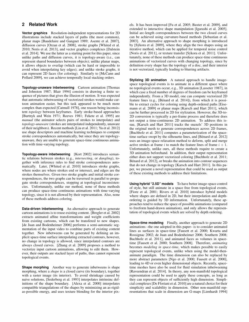
2 Related Work

Vector graphics Resolution-independent representations for 2Dillustrations include stacked layers of paths (the most common),planar maps [Baudelaire and Gangnet 1989; Asente et al. 2007],diffusion curves [Orzan et al. 2008], stroke graphs [Whited et al.2010; Noris et al. 2013], and vector graphics complexes [Dalsteinet al. 2014]. We use the latter as a starting point for this paper, sinceunlike paths and diffusion curves, it is topology-aware (i.e., canrepresent shared boundaries between objects); unlike planar maps,it allows objects to overlap (which can be hard or impossible toavoid when interpolating key edges); and unlike stroke graphs, itcan represent 2D faces (for coloring). Similarly to [McCann andPollard 2009], we can achieve temporally local stacking orders.

Topology-unaware inbetweening Cartoon animation [Thomasand Johnston 1987; Blair 1994] consists in drawing a finite se-quence of pictures that gives the illusion of motion. It was expectedthat automatic inbetweening of vectorized strokes would make car-toon animation easier, but this task appeared to be much morecomplex than expected [Catmull 1978], one reason being inconsis-tent topology between keyframes. Early stroke-based approaches[Burtnyk and Wein 1971; Reeves 1981; Fekete et al. 1995] aremanual (the animator selects pairs of strokes to interpolate) andtopology-unaware (strokes are interpolated independently, unawareof their neighbors). Recent methods [Liu et al. 2011; Yu et al. 2012]use shape descriptors and machine learning techniques to computestroke correspondences automatically, but since they are topology-unaware, they are unable to generate space-time continuous anima-tion with time-varying topology.

Topology-aware inbetweening [Kort 2002] introduces seman-tic relations between strokes (e.g., intersecting, or dangling), to-gether with inference rules to find stroke correspondences auto-matically. Later, [Whited et al. 2010] introduces stroke graphs,where nodes are where strokes end or intersect, and edges are thestrokes themselves. Given two stroke graphs and initial stroke cor-respondences, the two graphs can be traversed in parallel to propa-gate stroke correspondences, stopping at topological inconsisten-cies. Unfortunately, unlike our method, none of these methodscan produce space-time continuous animations with time-varyingtopology, since it is not allowed by their representation. Also, noneof these methods address coloring.

Data-driven inbetweening An alternative approach to generatecartoon animations is to reuse existing content. [Bregler et al. 2002]extracts animated affine transformations and weight coefficientsfrom existing cartoons, which can be transfered to new shapes.[de Juan and Bodenheimer 2006] performs a semi-automatic seg-mentation of the input video to combine parts of existing contenttogether. New inbetweens can be generated by defining an im-plicit space-time surface interpolating extracted contours, however,no change in topology is allowed, since interpolated contours arealways closed curves. [Zhang et al. 2009] proposes a method tovectorize input cartoon animations, allowing to edit them. How-ever, their outputs are stacked layer of paths, thus cannot representtopological events.

Shape morphing Another way to generate inbetweens is shapemorphing, where a shape is a closed curve (its boundary), togetherwith a raster image (its interior). To avoid shrinkage caused bynaive solutions, [Sederberg et al. 1993] interpolates intrinsinc def-initions of the shape boundary. [Alexa et al. 2000] interpolatescompatible triangulations of the shapes by minimizing an as-rigid-as-possible energy, and uses texture blending for the interior pix-

els. It has been improved [Fu et al. 2005; Baxter et al. 2009], andextended to interactive shape manipulation [Igarashi et al. 2005].Initial arc-length correspondences between the two closed curvescan be achieved using curvature-based methods [Sebastian et al.2003]. An alternative approach to shape morphing is introducedby [Sýkora et al. 2009], where they align the two shapes using aniterative method, which can be applied for temporal noise control[Noris et al. 2011], or texture transfer [Sýkora et al. 2011]. Unfor-tunately, none of these methods can produce space-time continuousanimations of vectorized curves with changing topology, since bydefinition every shape has the topology of a disc, and their interioris not vectorized, typically leading to blurring artifacts.

Stylizing 3D animation A natural approach to handle image-space topological events is to animate in a different space whereno topological events occur, e.g., 3D animation [Lasseter 1987], inwhich case a fixed number of degrees of freedom can be keyframedindependently. From a 3D model, one can compute vectorized 2Dfeature lines (e.g., [Bénard et al. 2014]), from which it is possi-ble to extract cycles for coloring using depth-ordered paths [Eise-mann et al. 2009] or planar maps [Karsch and Hart 2011], whichcan be further processed in 2D for stylization. However, the 3D-to-2D conversion is typically a per-frame process and therefore doesnot output a time-continuous 2D animation. To address this is-sue, [Karsch and Hart 2011] tracks the snaxels’ 3D positions inthe original mesh to generate correspondences across 2D frames,[Buchholz et al. 2011] computes a parameterization of the space-time surface swept by the silhouette lines, and [Bénard et al. 2012]uses an image-space relaxation method to deform, split and mergeactive strokes at frame i to match the feature lines of frame i + 1.Unfortunately, unlike ours, all these methods require to create a3D animation beforehand. In addition, their output representationeither does not support vectorized coloring [Buchholz et al. 2011;Bénard et al. 2012], or breaks the animation into contour sequencesthat do not change in topology [Karsch and Hart 2011]. In this pa-per, we present a novel representation that could be used as outputof these existing methods to address their limitations.

Using hybrid “2.5D” models To have better image-space controlof style, but still animate in a space free from topological events,[Fiore et al. 2001; Rivers et al. 2010] introduce hybrid modelswhere shapes are defined in 2D, but their interpolation and depth-ordering is guided by 3D information. Unfortunately, these ap-proaches tend to reduce the space of possible animations (comparedto freeform hand-drawn animation), and only allows the represen-tation of topological events which are solved by depth ordering.

Space-time modeling Finally, another approach to generate 2Danimations –the one adopted in this paper– is to consider animatedlines as surfaces in space-time [Fausett et al. 2000; Kwarta andRossignac 2002; de Juan and Bodenheimer 2006; Southern 2008;Buchholz et al. 2011], and animated faces as volumes in space-time [Fausett et al. 2000; Southern 2008]. Therefore, animatingbecomes modeling in space-time, which makes possible to easilyrepresent topological events, unlike when using the model-then-animate paradigm. The time dimension can also be replaced bymore abstract parameters [Ngo et al. 2000; Fausett et al. 2000],leading to 4D or even higher dimensional objects. Recently, space-time meshes have also be used for fluid simulation inbetweening[Raveendran et al. 2014]. In theory, any non-manifold topologicalrepresentation could be used to apply these concepts, as long asthey can represent objects of sufficiently high dimension. Simpli-cial complexes [De Floriani et al. 2010] are a natural choice for theirsimplicity and scalability in dimension. Other non-manifold rep-resentations that scale in dimension are G-maps [Lienhardt 1994]

Sequential keyframing Topological keyframing

value

time

value

time

[(t1, p1); (t2, p2); (t3, p3); (t4, p4)]

[(t′1, p′1); (t

′2, p

′2)]

[(t′′1 , p′′1 ); (t

′′2 , p

′′2 ); (t

′′3 , p

′′3 )]

{v1 = (t1, p1), . . . , v7 = (t7, p7)}

{v1 = (v1, v3), . . . ,v6 = (v2, v6)}

v1v2

v3

v4

v5

v6

v7

Figure 2: Left: The existing keyframing paradigm, defining an an-imation as ordered sequences of key values. Right: Our more gen-eral approach, where key values are unordered but labeled, andinbetween values specify which one to interpolate.

and the selective geometric complex [Rossignac and O’Connor1989]. If no more than three dimensions are needed, the radial-edge[Weiler 1985] or handle-cell [Pesco et al. 2004] structures could beappropriate choices as well. Unfortunately, none of these represen-tations are designed to represent space-time objects, and while theycan be very appropriate for algorithm processing, artistic space-time modeling using them is particularly non intuitive. What makesour representation unique is that it treats the time dimension sepa-rately from the space dimensions, enabling a keyframing paradigmsimilar to what animators are familiar with. For instance, insteadof a 1D entity called “edge”, we make the distinction between twotypes of 1D entities: a key edge (1D in space; 0D in time) representsan edge at a given time, and an inbetween vertex (0D in space; 1Din time) represents an interpolation between two key vertices. Eventhough they are both 1D in space-time, they are created, edited, andvisualized differently, reflecting a cleaner semantics.

3 Space-Time Topology

In this section, we provide an initial intuition behind the vector an-imation complex, which we formally define in Section 4.

3.1 Animating vertices

Suppose an animator wants to create a time-continuous animationof a single vertex v. This means that he needs to define its po-sition p(t) for every time t in the life-span of the vertex. Theexisting approach (Fig. 2, Left) is to define a sequence of keys[(t1, p1); (t2, p2); . . . ] which are interpolated in time. To animatethree vertices, the animator would define three sequences of keys.Let us call this paradigm sequential keyframing, since the repre-sentation is a set of sequences of keys: one sequence per animatedvertex, or more generally, one per animated degree of freedom.

But what if the animator wants the number of vertices –or degreesof freedom– to change over time, by splitting or merging? We canobserve (Fig. 2, Right) that the space-time topology of such ani-mation is not anymore disconnected sequences, but a more generalgraph. Therefore, sequential keyframing fails to represent such an-imation with time-varying topology, and we need a more generalapproach to keyframing that we call topological keyframing. Theanimator first defines a set of key vertices vi = (ti, pi), as in se-quential keyframing except that they are not ordered in sequences.Then, he defines a set of inbetween vertices vj = (vbefore, vafter)that reference to two key vertices to interpolate.

In theory, such paradigm can easily be applied to animate any kindof values, say, quaternions. However, in this paper, we use it toanimate the topology of vector graphics illustrations. This poses

time

space

edgegrowing

fromvertex

keyframe edgebeingcut

partialkeyframes

edgedisappearing

edgebeing

duplicated

Figure 3: Stroke graph animation with time-varying topology. Reddots are key vertices; (non-vertical) red curves are inbetween ver-tices; (vertical) blue curves are key edges; and light blue areas areinbetween edges. Each annotation describes either a topologicalevent introduced by key cells, or specifies that key cells are used asconventional “keyframes” (trajectory control, no change in topol-ogy). Note: key edges are represented as straight lines (becausespace is represented as 1D), but are in fact general 2D curves.

before

start animated vertex

end animated vertex

Inbetween open edge Inbetween closed edge

pathafterpath

beforecycle

aftercycle

Figure 4: Topology of inbetween edges. Note: a path or cycle canalso consist of a single key vertex (but an animated vertex cannot).A cycle can also consist of a single closed edge, possibly repeated.

additional challenges due to the fact that such topology is already agraph-like structure in the space dimension. Therefore, we have torepresent incidence relationships both in the temporal domain andthe spatial domain, resulting in a space-time complex.

3.2 Animating stroke graphs

Suppose now that we want to animate a stroke graph [Whited et al.2010], i.e. not only vertices but also (open) edges, which are 2Dcurves starting at a start vertex and ending at an end vertex. Aneasy way to achieve this is to define first a stroke graph, then usesequential keyframing to animate independently its degrees of free-dom (e.g., position of the vertices and Bézier control points of theedges). Unfortunately, with this approach, it is impossible to repre-sent animated stroke graphs with time-varying topology.

Our solution (Fig. 3) is to represent such animation as a space-timecomplex made of key vertices and inbetween vertices (as definedpreviously), but also key edges and inbetween edges. A key (open)edge ei is defined by a time ti and a 2D curve φi(s), starting at a keyvertex vstart = (ti, p1) and ending at a key vertex vend = (ti, p2).An inbetween (open) edge ej is defined by its temporal bound-ary and its spatial boundary (detailed in the next paragraph), fromwhich can be computed a time-parameterized 2D curve Φ(s, t) (i.e.,a surface in space-time) interpolating this boundary.

vstart

vend

e before

e after

Naively (Fig. opposite), one might define thetemporal boundary as a pair (ebefore, eafter)that references to two key edges to interpolate,and the spatial boundary as a pair (vstart,vend)that references to two inbetween vertices where

the time-parameterized curve Φ(s, t) should start and end (for tfixed). Unfortunately, this naive definition would only enable to

represent a very small subset of all possible topological events thatcan happen to a stroke graph, and therefore we need a more gen-eral definition (Fig. 4, Left). Indeed, to represent an edge beingcut in half by an appearing vertex (Fig. 3), or cut in more piecesby several vertices appearing simultaneously, we need the temporalboundary not to be two key edges, but two “sequences of connectedkey edges”, structure that we call path. To represent an edge grow-ing from a vertex, we need to allow paths to be reduced to a keyvertex. Finally, To allow partial keyframing (e.g., adding a key toan inbetween edge without adding a key to every incident edge, andrecursively to every connected edge), we need the spatial bound-ary not to be two inbetween vertices, but two “sequences of con-nected inbetween vertices”, structure that we call animated vertex(it is a chain key—inbetween—key—· · ·—key—inbetween—key,which can be interpreted as a vertex animated using conventionalkeyframing).

3.3 Animating vector graphics complexes

We extend these ideas further to represent an animated vectorgraphics complex [Dalstein et al. 2014] with time-varying topol-ogy. The same way that the VGC extends stroke graphs with closededges and faces, the VAC extends the representation introduced inthe previous section with key closed edges, inbetween closed edges,key faces, and inbetween faces.

A key closed edge ei is defined by a time ti and a 2D closed curveφi(s) (note that is does not have bounding vertices). An inbe-tween closed edge ej is defined by its temporal boundary, madeof two cycles (Fig. 4, Right), from which can be computed a time-parameterized 2D closed curve Φ(s, t) interpolating this boundary.Note that unlike inbetween open edges, inbetween closed edgeshave an empty spatial boundary, since closed edges do not havebounding vertices. To allow all sorts of topological events, cyclescan either be reduced to a single key vertex, or made of a single(possibly repeated) key closed edge, or made of connected key openedges.

A key face fi is defined by a time ti and a sequence of cycles,all sharing the same time ti. Given a winding rule (e.g., even-odd or non-zero), these cycles define a 2D region of the time-planet = ti. An inbetween face fj is defined by its temporal boundaryand its spatial boundary. Its temporal boundary is defined by twosequences of faces, the before faces and the after faces. Its spatialboundary is defined by a sequence of animated cycles, structurethat we introduce informally in the next three paragraphs.

Animated cycle We have seen that an animated vertex is a com-binatorial structure that stores references to existing inbetween ver-tices, which define a time-parameterized position p(t). Similarly,our goal is now to define a time-parameterized closed curve Φ(s, t),via a combinatorial structure storing references to existing cells (a“cylinder in space-time”, cf. Fig. 5, Top-left). A simple optionwould be to define this boundary as a set {c1, . . . , cn} of refer-ences to cells. However, for the same reasons that this approachfails to define the boundary of key faces (cf. [Dalstein et al. 2014]),this approach fails to define the boundary of inbetween faces too.More specifically, because overlapping of cells is allowed (i.e., thecomplex is only immersed in space-time, as opposed to embedded),then the set of boundary cells does not contain enough informationto unambiguously define the geometry of the face. Instead, it isnecessary to organize this set using an ordered structure, possiblyrefering to the same cell multiple times. This additional informa-tion explicitly defines a parameterization of the boundary. For keyfaces, this is achieved via the structure called cycle. For inbetweenfaces, this is achieved via the structure called animated cycle.

e1, β1next

previous

after before

e2, β2

e3, β3 e4, β4

e1 e2

e3e4

timet

curve parameter s

cell geometry and animated cycle•γ

incidence relationship

e1, β1 e2, β2

e3, β3 e4, β4

(naive data structure)

animated cycle•γ

(actual data structure)

Figure 5: Top: Intuitively, an animated cycle•γ is a two-

dimensional doubly linked list where every node holds a referenceto an inbetween edge and an orientation. The structure is circu-lar in the space dimension, and non-circular in the time dimen-sion. Unfortunately, this naive structure is not expressive enough tocapture all possible scenarios. Bottom: The actual data structureincludes additional nodes to explicitly hold a reference to sharedvertices, key edges, and inbetween vertices.

Intuitively (Fig. 5, Top-right), a naive structure to define such pa-rameterization would be a two-dimensional doubly linked list oforiented inbetween edges, where the first dimension correspondsto the curve parameter s, and the second dimension correspond tothe time t. This structure is circular in the s-dimension, but non-circular in the t-dimension. Like a doubly linked list, it is com-posed of nodes which store: 1) per-node data; and 2) references toadjacent nodes. But unlike a doubly linked list, each node storesfour references instead of two: previous and next to navigate in thes-dimension; and before and after to navigate in the t-dimension.The node data itself is a reference to an inbetween edge e, and aboolean β that orients e with respect to curve parameterization.

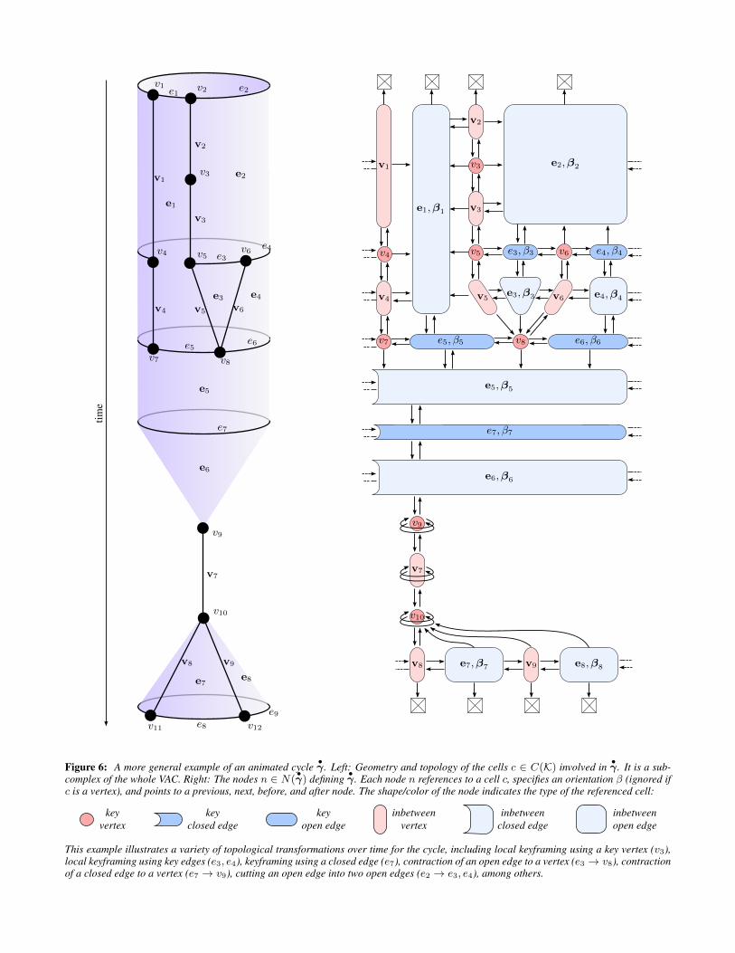
Unfortunately, this naive structure cannot handle inbetween edgesbounded by more than two key edges, more than two inbetweenvertices, or that shrink to a key vertex, and thus cannot representgeneral time-parameterized cycles (e.g., Fig. 6, Left). Our solu-tion is to include all the lower dimensional cells shared betweeninbetween edges as explicit nodes of the structure (Fig. 5, Bottom;Fig. 6, Right). It introduces a little redundancy to the structure, butmakes it significantly more expressive.

4 Formal Definition

A vector animation complex K is defined as a tuple

K = (C, dimT , dimS , . . . ) (1)

where C is a finite set of abstract symbols called cells (think ofthem as identifiers, or addresses), and dimT , dimS , . . . are func-tions defined onC or a subset ofC, assigning to relevant cells someattributes, that have to satisfy some invariants. These numerous at-tributes and invariants are detailed in the remainder of this section.In our C++ implementation, an element c ∈ C is a pointer to anobject inheriting the class Cell, and an attribute α(c) is typicallya data member c->m_alpha.

Cell attributes can be classified in two types: topological attributes,which are combinatorial objects defining incidence relationship be-tween cells; and geometrical attributes, which are continuous ob-jects immersing the cells in space-time. The two most importantattributes of any cell c ∈ C are topological:

• its temporal dimension dimT (c) ∈ {0, 1}• its spatial dimension dimS(c) ∈ {0, 1, 2}

Cells of temporal dimension 0 are called key cells, and cells of tem-poral dimension 1 are called inbetween cells. Orthogonally, cellsof spatial dimension 0 are called vertices, cells of spatial dimen-sion 1 are called edges, and cells of spatial dimension 2 are calledfaces. In addition, each edge e is assigned the topological attributeisClosed(e) ∈ {true, false}. Therefore, the cells in C can be par-titionned into eight finite sets which define their type:

dimT dimS isClosed Type Notation

0 0 n/a key vertex v ∈ V0 1 true key closed edge e ∈ E◦0 1 false key open edge e ∈ E|0 2 n/a key face f ∈ F

1 0 n/a inbetween vertex v ∈ V1 1 true inbetween closed edge e ∈ E◦1 1 false inbetween open edge e ∈ E|1 2 n/a inbetween face f ∈ F

For convenience, we define E = E| ∪ E◦ and E = E| ∪ E◦. InSection 4.1, we define all the remaining attributes and invariants foreach type of cells. For clarity, some of these attributes are expressedusing auxiliary structures (halfedges, paths, cycles, animated ver-tices, and animated cycles), which are defined in Section 4.2.

4.1 Cell attributes and invariants

Key vertex A key vertex v ∈ V represents a single point inspace-time:

topological attributes: ∅geometrical attributes: position p(v) ∈ R2

time t(v) ∈ Rinvariants: ∅

Key closed edge A key closed edge e ∈ E◦ represents a closedcurve contained in a time-plane:

topological attributes: ∅geometrical attributes: curve φ(e) : s ∈ [0, 1]→ R2

time t(e) ∈ Rinvariants: φ(e) continuous

φ(e)(0) = φ(e)(1)

Key open edge A key open edge e ∈ E| represents an opencurve contained in a time-plane, starting and ending at two key ver-tices (possibly equal):

topological attributes: start vertex vstart(e) ∈ Vend vertex vend(e) ∈ V

geometrical attributes: curve φ(e) : s ∈ [0, 1]→ R2

time t(e) ∈ Rinvariants: φ(e) continuous

φ(e)(0) = p(vstart(e))φ(e)(1) = p(vend(e))

t(vstart(e)) = t(e) = t(vend(e))

Key face A key face f ∈ E represents a region of a time-planedelimited by closed curves (possibly self-intersecting, including go-ing back and forth the same path or being reduced to a single point):

topological attr: cycles ∀i ∈ [1..k(f)], γi(f) ∈ Γ

where k(f) ≥ 0

geometrical attr: winding rule R(f) ⊆ Ntime t(f) ∈ R

invariants: ∀i ∈ [1..k(f)], t(f) = t(γi(f))

Inbetween vertex An inbetween vertex v ∈ V represents aninterpolation in time between two key vertices:

topological at.: before vertex vbefore(v) ∈ Vafter vertex vafter(v) ∈ V

geometrical at.: animated position p(v) : t ∈ [t1, t2]→ R2

where t1 = t(vbefore(v))t2 = t(vafter(v))

invariants: t1 < t2

p(v) continuousp(v)(t1) = p(vbefore(v))p(v)(t2) = p(vafter(v))

Inbetween closed edge An inbetween closed edge e ∈ E◦ rep-resents an interpolation in time between two cycles:

t. at.: before cycle γbefore(e) ∈ Γafter cycle γafter(e) ∈ Γ

g. at.: animated curve Φ(e) : (s, t) ∈ [0, 1]× [t1, t2]→ R2

where t1 = t(γbefore(e))t2 = t(γafter(e))

inv.: t1 < t2

Φ(e) continuous∀t ∈ [t1, t2],Φ(e)(0, t) = Φ(e)(1, t)

∀s ∈ [0, 1],Φ(e)(s, t1) = φ(γbefore(e))(s)∀s ∈ [0, 1],Φ(e)(s, t2) = φ(γafter(e))(s)

Inbetween open edge An inbetween open edge e ∈ E| repre-sents an interpolation in time between two paths, spatially boundedby two animated vertices:

t. at.: before path πbefore(e) ∈ Πafter path πafter(e) ∈ Π

start animated vertex•vstart(e) ∈

•V

end animated vertex•vend(e) ∈

•V

g. at.: animated curve Φ(e) : (s, t) ∈ [0, 1]× [t1, t2]→ R2

where t1 = t(πbefore(e))t2 = t(πafter(e))

inv.: vstart(πbefore(e)) = vbefore(•vstart(e))

vend(πbefore(e)) = vbefore(•vend(e))

vstart(πafter(e)) = vafter(•vstart(e))

vend(πafter(e)) = vafter(•vend(e))

t1 < t2

Φ(e) continuous∀t ∈ [t1, t2],Φ(e)(0, t) = p(

•vstart(e))(t)

∀t ∈ [t1, t2],Φ(e)(1, t) = p(•vend(e))(t)

∀s ∈ [0, 1],Φ(e)(s, t1) = φ(πbefore(e))(s)∀s ∈ [0, 1],Φ(e)(s, t2) = φ(πafter(e))(s)

Inbetween face An inbetween face f ∈ F represents an inter-polation in time between key faces, spatially bounded by animatedcycles:

top. at.: before time tbefore(f) ∈ Rbefore faces ∀i ∈ [1..kb(f)], fbefore,i(f) ∈ F

where kb(f) ≥ 0

after time tafter(f) ∈ Rafter faces ∀i ∈ [1..ka(f)], fafter,i(f) ∈ F

where ka(f) ≥ 0

animated cycles ∀i ∈ [1..k(f)],•γi(f) ∈

•Γ

where k(f) ≥ 0

geo. at.: winding rule R(f) ⊆ N

inv.: ∀i ∈ [1..kb(f)], tbefore(f) = t(fbefore,i(f))∀i ∈ [1..ka(f)], tafter(f) = t(fafter,i(f))

∀i ∈ [1..k(f)], tbefore(f) = tbefore(•γi(f))

∀i ∈ [1..k(f)], tafter(f) = tafter(•γi(f))

4.2 Auxiliary structures

Halfedge A halfedge is a pair h = (e, β) ∈ E × {>,⊥}. If e isclosed then it is a closed halfedge denoted h ∈ H◦, otherwise it isan open halfedge denoted h ∈ H|. If β = >, we define φ(h)(s) =φ(e)(s), otherwise we define φ(h)(s) = φ(e)(1− s). If h is openthen we define vstart(h) = vstart(e) and vend(h) = vend(e) (whenβ = >), or vstart(h) = vend(e) and vend(h) = vstart(e) (whenβ = ⊥). Finally, we define t(h) = t(e).

Path A path π is either:

1. a key vertex v ∈ V , or2. a list of N > 0 open halfedges h1, .., hN ∈ H| satisfying:

∀j ∈ [1..N − 1], vend(hj) = vstart(hj+1)

In the first case, we define vstart(π) = vend(π) = v, otherwisewe define vstart(π) = vstart(h1) and vend(π) = vend(hN ). Also,we define the curve φ(π) : s ∈ [0, 1] → R2 by concatenating anduniformly reparameterizing the φ(hj). In the special case π = v,then φ(π) is the constant function Φ(π)(s) = p(v). Finally, wedefine t(π) = t(v) (Case 1.), or t(π) = t(h1) (Case 2.). We denoteby Π the set of all possible paths on K.

Cycle A cycle γ is either:

1. a key vertex v ∈ V , or2. a closed halfedge h ∈ H◦ repeated N > 0 times, or

3. a circular list of N > 0 open halfedges hj ∈ H| satisfying:

∀j ∈ [1..N ], vend(hj) = vstart(hj+1)

In addition, a cycle stores a starting point s0 ∈ R. We definethe closed curve φ(γ) : s ∈ [0, 1] → R2 by concatenating anduniformly reparameterizing the φ(hj), then offsetting by s0. In thespecial case γ = v, then φ(γ) is the constant function Φ(γ)(s) =p(v). Finally, we define t(γ) = t(v) (Case 1.), or t(γ) = t(h)(Case 2.), or t(γ) = t(h1) (Case 3.). We denote by Γ the set of allpossible cycles on K.

Animated vertex An animated vertex•v is a list of N > 0 inbe-

tween vertices v1, ..,vN ∈ V satisfying:

∀j ∈ [1..N − 1], vafter(vj) = vbefore(vj+1)

We define vbefore(•v) = vbefore(v1) and vafter(

•v) = vafter(vN ).

Also, we define the time-parameterized position p(•v) : t ∈

[t(vbefore(•v)), t(vafter(

•v))] → R2 by concatenating the p(vj).

We denote by•V the set of all possible animated vertices on K.

Animated cycle An animated cycle is a tuple•γ = (N, c, β, nprevious, nnext, nbefore, nafter) (2)

where N is a non-empty set of symbols called nodes, and:

c : N → V ∪V ∪ E ∪E assigns a cell to every node

β : N → {>,⊥} assigns an orientation(ignored if c(n) ∈ V ∪V)

nprevious : N → N assigns a previous node

nnext : N → N assigns a next node

nbefore : N → N ∪ {null} assigns an optional before node

nafter : N → N ∪ {null} assigns an optional after node

In addition, an animated cycle stores a starting node n0 ∈ N .We define the timespan of a node n as being the trivial inter-val T (n) = {t(c(n))} if c(n) is a key cell, or the open intervalT (n) = (tbefore(c(n)), tafter(c(n))) if c(n) is an inbetween cell.Despite having a single next pointer, one can notice (Fig. 6) thatwhen c(n) is an inbetween open edge, then n may have severalnodes “next to it”, which are stacked in time. The next (resp. pre-vious) pointer points to the “first” of these, and the others can beaccessed by iterating after (resp. before). To easily traverse thedata-structure at t fixed, we define the two functions nnext(n, t)and nprevious(n, t) that return the two nodes “spatially adjacent ton at time t”.

nprevious(n ∈ N , t ∈ R)

Require: t ∈ T (n)n′ ← nprevious(n)while t 6∈ T (n′) do

n′ ← nbefore(n′)

return n′

nnext(n ∈ N , t ∈ R)

Require: t ∈ T (n)n′ ← nnext(n)while t 6∈ T (n′) do

n′ ← nafter(n′)

return n′

We define the time-parameterized closed curve Φ(•γ)(s, t) by find-

ing a node n such that t ∈ T (n) (iterating before/after from n0),then concatenating the φ(c(n)) while iterating nnext(n, t) (fol-

lowed by a normalization into [0, 1]). We denote by•Γ the set of

all valid animated cycles on K, which are the ones whose attributessatisfy the invariants that we provide in supplemental material, to-gether with the definition of tbefore(

•γ) and tafter(

•γ).

time

v1 v2

v3

v4 v5v6

v7 v8

v9

v10

v11 v12

e1 e2

e3e4

e5e6

e7

e8e9

v1

v2

v3

v4 v5 v6

v7

v8 v9

e1

e2

e3 e4

e5

e6

e7e8

v2

v3

v3

v5

v5

v8

e5,β5

e7, β7

v9

v7

v10

v8

v1

v4

v4

v7

e1,β1

v6e3,β3 e4,β4

e2,β2

v6e3, β3 e4, β4

e5, β5 e6, β6

e6,β6

v9e7,β7 e8,β8

Figure 6: A more general example of an animated cycle•γ. Left: Geometry and topology of the cells c ∈ C(K) involved in

•γ. It is a sub-

complex of the whole VAC. Right: The nodes n ∈ N(•γ) defining

•γ. Each node n references to a cell c, specifies an orientation β (ignored if

c is a vertex), and points to a previous, next, before, and after node. The shape/color of the node indicates the type of the referenced cell:

keyvertex

keyclosed edge

keyopen edge

inbetweenvertex

inbetweenclosed edge

inbetweenopen edge

This example illustrates a variety of topological transformations over time for the cycle, including local keyframing using a key vertex (v3),local keyframing using key edges (e3, e4), keyframing using a closed edge (e7), contraction of an open edge to a vertex (e3 → v8), contractionof a closed edge to a vertex (e7 → v9), cutting an open edge into two open edges (e2 → e3, e4), among others.

(a) (b) (d) (e)(c)

Figure 7: Interpolation scheme (time = horizontal axis). (a) Input:geometry of key cells and space-time topology. (b) Compute tan-gents at key vertices. (c) Compute geometry of inbetween vertices,satisfying tangents. (d) For each inbetween edge, compute linearinterpolation of bounding paths/cycles. (e) Output: warp to satisfyspatial boundary conditions.

5 Interpolation Scheme

The geometry of inbetween cells may be provided explicitly (or innon-photorealistic rendering applications, computed from an ani-mated 3D model), but in our case, it is computed by interpolatingthe geometry of key cells, as expected from a keyframing system.

First, for each key vertex vi, we define a tangent q(vi) as the av-erage of the slopes p(vj)−p(vi)

t(vj)−t(vi), for all key vertices vj connected

to vi by an inbetween vertex (Fig. 7b). Then, we define the ge-ometry of each inbetween vertex as the unique cubic curve inter-polating the positions p(vbefore) and p(vafter) with the desired tan-gents q(vbefore) and q(vafter) (Fig. 7c). All that is left to do isdefine the geometry of every inbetween open (resp. closed) edge,by interpolating its two bounding paths (resp. cycles). We recallfrom Section 4 that paths/cycles have an explicit parameterization[0, 1]→ R2, obtained by concatenating and uniformly reparameter-izing the key edges’ parameterizations (the starting point of cyclesis a user-controllable variable). First, we compute a linear interpola-tion between these two explicit parameterizations (Fig. 7d). Finally,in the case of inbetween open edges, for all t ∈ (t1, t2), we linearlywarp this interpolation Φ(s, t) such that Φ(0, t) and Φ(1, t) coin-cidate with the start and end animated vertices at t (Fig. 7e). Thereis no need to define an interpolation scheme for inbetween faces,since their geometry is entirely specified by the geometry of theirboundary. Indeed, for all t ∈ (t1, t2), a closed parameterized curve[0, 1]→ R2 can be extracted from each animated cycle, which, to-gether with the user-specified winding rule (e.g., even-odd), definean area of the 2D plane.

This interpolation scheme is robust and general but limited as it onlyguarantees C0 continuity. More aesthetically pleasing interpolationcan be achieved using logarithmic spirals [Whited et al. 2010] orCoons patches. This is left for future work.

6 User Interface

To create and manipulate VACs, we implemented various visualiza-tions and topological operators, which we present in this section.We refer to the accompanying video for a demonstration of thesetools.

2D view We provide a 2D view to render a specific frame of theanimation (i.e., a time-slice of the VAC), which can be selectedusing a timeline similar to any animation system. The 2D view canbe split into multiple 2D views to visualize simultaneously differentframes of the animation. The user can also toggle “onion skinning”to overlay several frames within a single 2D view, or render theanimation as an animation strip (Fig.1, bottom). The frames can berendered either in “normal” mode (showing the actual result), or in“topology” mode (using a color code to inform whether a cell is akey cell, or a time-slice of an inbetween cell).

3D view We also provide a 3D view to visualize the VAC inspace-time. However, we mostly use this view as a debugging tool,as it becomes quickly impractical when the number of cells grow.All interaction happens in the 2D views, and all examples presentedin this paper have been created without using the 3D view at all. Atthis stage, it is unclear whether it is relevant to expose such visual-ization to end users.

Creating key cells Key cells are created in the 2D view usingstandard VGC tools. They are assigned the time ti selected in thetimeline.

Motion-pasting The easiest way to create inbetween cells is toselect key cells at time t1, trigger the copy action, then move totime t2 and trigger the motion-paste action. It creates a copy of thekey cells, assigns them the time t2, and creates inbetween cells thatconnect in time the old key cells to the new ones. In other words, itcorresponds to sweeping key cells in time. Once motion-pasted, thenew cells can be edited to create the desired motion. Standard VGCtopological operators (extended to support incident inbetween cells)can also be used on the new key cells, which introduce topologicalevents as a result.

Inbetweening Another way to create inbetween cells is to selectexisting key cells at two different times t1 and t2 (e.g., using side-by-side 2D views), then trigger the inbetweening action. It createsinbetween cells that connect in time the selected key cells. Cur-rently, it works to create an inbetween vertex out of two key ver-tices; an inbetween edge out of two key edges; an inbetween edgeout of more than two key edges that can be organized into two pathsor two cycles; or an inbetween edge that grows or shrinks to a ver-tex. This tool does not yet support the creation of inbetween faces(we can still create them using motion-pasting or manually speci-fying their boundary), neither the simultaneous creation of multipleinbetween edges, which are both interesting challenges left as fu-ture work.

Inserting keys A fundamental topological operator on VACs isto cut an inbetween cell in half, in the time dimension, by inserting anew key cell. It is the equivalent of inserting a keyframe in conven-tional keyframing animation. Similarly to the “auto-key” feature ofmost animation systems, we automatically call this operator when-ever the user performs an action on (the rendered time-slice of) aninbetween cell. For instance, attempting to move an inbetween ver-tex automatically inserts a key vertex at the time ti selected in thetimeline, and the new key vertex is the cell actually moved. Notethat this insert key tool is local: it cuts the selected inbetween celland its spatial boundary, but does not propagate to any other cell.This allows for local trajectory or topology refininement possible,without keyframing the whole drawing.

Drag-and-drop Selected key cells can be drag-and-dropped inspace (using the 2D view), but also in time (using the timeline),within a time interval determined by its incident inbetween cells.This allows to easily refine the timing of a motion.

Depth-ordering We store a global ordering for all the cells ina complex using a doubly-linked list, and render the cells back-to-front using this ordering. As with VGCs, we provide tools toconveniently alter this ordering.

Figure 8: Double Torus.

A B C D C D C D E F G H G H G H I J

Figure 9: Animated ribbon decomposed into 6 key faces(A,B,E,F,I,J) and 4 inbetween faces (C,D,G,H), in order to depictlocal depth-ordering both in space and time.

7 Results

We create several illustrative examples of vector graphics anima-tions that involve topological changes over time. We briefly sum-marize them below, although they are best seen in the video thataccompanies this paper.

Torus The torus (Fig. 1) is an example use of the VAC to cre-ate a clean conceptual animated vector graphics illustration. It isdefined using a total of five keyframes (frames that contain at leastone key cell). As always required, the clip begins and ends withfull keyframes (frames containing key cells only), which specifythe shape of all the drawing elements that exist at those key times.The second keyframe captures the motion of the interior silhou-ette, marks the initial appearance of the hole with a single vertex,and also keyframes the shape of the outside silhouette. The thirdkeyframe properly introduces the now-visible hole, while the fourthkeyframe then ends the growth of the hole by merging the end ver-tices of the two lines. As seen in this example, keyframes are usedeither to introduce a change in shape, to introduce a change in topol-ogy, or both. Keyframes are typically local, i.e., key cells are onlyinserted where needed, without keyframing the entire drawing.

Double torus Once we have the VAC for the single torus, the an-imation of a double torus (Fig. 8) is easy to create. Indeed, all thatis needed is: 1) deforming the outside silhouette, 2) copy-pastingto a different space-time location the sub-complex representing theanimation of the hole, and 3) gluing the first key edge of this sub-complex to the deformed silhouette. We believe that this type oftemplate-based construction provides a practical way of simplifyingthe creation of VACs. Figure 8 shows a vector graphics animationof a simple torus which is morphed to a double torus, with the twohalves rotating asynchronously. Creating such animation would behard using conventional vector graphics tools, but would be equallyhard in 3D, since the genus of the depicted surface changes, requir-ing a topological event in 3D as well.

Animated ribbon In a given VAC, any cell is either completelyin front, or completely behind, any other cell. However, any cellcan be easily split spatially (cutting) or temporally (keyframing)into different cells, and the cells of this new cell-decomposition areassigned their own independent depth orders. This makes possible

Figure 10: Bird animation. Space-time view (top); output anima-tion (middle); VGC film strip (bottom).

to depict local depth-ordering, both in space and time, as illustratedin Figure 9. Using motion-pasting and basic editing, the space-timetopology and geometry of this animation can be created within afew seconds. Then, the user alters the depth-ordering to ensureA < B,C < D,G > H , and I > J , using the “raise” and “lower”actions, as with standard VGCs. Note that this example does notcontain topological events: keyframes are only used to introduce achange in geometry, as well as a change in depth-ordering.

Flapping bird We demonstrate Figure 10 the use of animatedfaces with depth layering in creating an example of a bird with aflapping wing, as inspired by a hand-drawn animation [Blair 1994,p. 122]. This example is created using 7 keyframes, all of whichare local except the ones at the start and end. A looping animationis easily created by copy-and-pasting a second copy of the full VACso that it sits immediately after the first copy. The ending elementsof the first animation are then topologically glued to the startingelements of the second animation.

Head turning We use a drawn animation sequence by JamesLopez (used with permission) as inspiration for a more complex ex-ample, shown in Figure 11. This involves many drawn elements anda significant number of topological changes, particularly involvingthe ear, goggles, eye, and mouth. Many topological changes neednot be modeled in great detail. The eye is a good example: the fea-tures of the eye are simply spawned from an initial vertex that isintroduced on the silhouette of the face. For this example, the 3Dspace-time view is largely unusable because of its complexity, andthus it proved to be a good test case for the capabilities of our userinterface.

Figure 11: Turning head animation. Output animation (top); VGCfilm strip (bottom).

8 Discussion

Creation Many aspects of working with the VAC are no differ-ent than that of creating a conventional keyframe animation. An-imation workflows are often classified as being straight ahead orpose-to-pose, and these working styles can each be reproduced us-ing the VAC. A straight ahead workflow is readily reproduced us-ing motion-pasting to create a new keyframe, followed by editingas necessary. A pose-to-pose workflow can be modeled by creatingindependent keyframes, followed by the creation of inbetween cellsinterpolating the key cells. For other potential applications, such asthe vectorization of existing animations or video clips, we expectthat the creation of the VAC may be automated.

Editing Creating the space-time topology of a complex animationmay take more time than via traditional animation but once created,the VAC offers significant benefits as it provides a compact repre-sentation that is continuous in space and time. The VAC can beeasily edited in ways that are not possible with traditional 2D or 3Danimation pipelines. The VAC also provides a compact and conve-nient representation for algorithms to operate on. For example, weenvision algorithms that can produce rich variations of an existinganimated drawing by adding stochastic perturbations in space andtime to some of the key elements.

Local keyframing Conventional keyframing animation allowsfor independent keyframing of the animation variables, i.e., thekeyframe times for an animated knee-joint motion can be differentfrom the keyframe times for the animated ankle motion within thesame animation. Similarly, the VAC allows for the asynchronousspecification of keyframes for portions of the vector graphics com-plex. Local keyframes provide better support for the semantics ofmany vector graphics drawings by allowing different portions of adrawing to be governed by different keyframes. It also allows formany topological changes to be conveniently modeled using instan-tiated templates.

Repurposing of exising 3D complexes It is tempting to be-lieve that modeling an animated 2D complex could be achievedusing existing approaches for 3D topological modeling, where thez-coordinate simply plays the role of time. Unfortunately, this doesnot reflect the unique semantics of the time axis, and this mani-fests itself in several ways. An “out of plane” rotation of a vec-tor graphics animation does not usually produce a valid anima-tion because the space is not Euclidean. For similar reasons, oth-

ers have proposed representing image spaces as a non-Euclidean,Cayley-Klein geometry with one isotropic dimension [Koenderinkand Doorn 2002]. Without a special designation for time, spe-cific strategies would be needed to model the changing depth-orderings that can be desired during the course of a vector graph-ics animation, and which, by contrast, are easily modeled usingthe VAC. More importantly, cells would not always admit a time-parameterization. By contrast, all cells in our complex have anexplicit time-parameterization, by design. This makes extractingtime-slices trivial and also guarantees that all topological events areconstrained to occur at key cells. This would not be the case if ourcells were allowed to do “switch-backs” in time. In addition, de-spite being both 1D in space-time, the distinction we make betweenkey edges and inbetween vertices is critical since their intersectionwith a time-plane is an object of different dimension. They mustthus be rendered differently and store different attributes. The sameis true for key faces and inbetween edges. Also, we allow zero-length edges but not zero-duration inbetween cells, i.e., we enforcet1 < t2. Similarly, paths are allowed to be reduced to a single keyvertex, while animated vertices are not.

Using a simplicial complex representation for vector graphics an-imation [Southern 2008] would necessitate the use of many cells,which could then be problematic for creation, editing, and vi-sualization, as well as being further removed from the standardkeyframing paradigm for animation. Given a simplicial complexthat completely reflects the geometry of an VAC, the VAC can beseen as inducing a partition of the simplicial complex, resulting inan output semantics similar to [Buchholz et al. 2011]. In general,geometric complexes allow for models and operations that we wishto forbid in order to reflect the unique nature of the time dimen-sion. Implementing the desired constraints necessitates additionalcomplexity while the VAC implements the desired constraints bydesign, i.e., as part of its desiderata. Also, we note that the inter-section of a 3D simplicial complex with a time-plane is not neces-sarily a 2D simplicial complex (as the intersection between a tetra-hedron and a plane can be a four-sided polygon). By contrast, theintersection of a VAC with a time-plane is guaranteed by designto be a VGC, which is trivial to compute due to the explicit time-parameterization.

Limitations While there are many benefits to a structure that pro-vides a sound, continuous-time model of the topological events invector graphics animations, it also comes with additional complex-ity. In particular, the modeling and editing of animated cycles, asrequired in order to animate faces in the vector graphics complex,embodies much of the complexity of the data structure and its im-plementation. The space-time topology is also likely to introduce asteep learning curve for artists coming from the world of SVG mod-els where changes in topology are approximated by other means.We currently leave the development of an improved user interfaceas future work, and as such we have not conducted a formal userstudy with regard to how end users can best work with the VAC.We believe that the use of topological-event templates may signifi-cantly simplify the workflow for modeling and editing. Finally, oursystem shares the same fundamental limitation of any 2D animationsystem: the loss of information between the depicted 3D world andthe 2D depiction [Catmull 1978]. In other words, the semantics ofa rotating 3D object will always be better captured by 3D represen-tations. We believe that the automatic computation of a VAC froman animated 3D model would alleviate this issue.

Future work The VAC opens up a number of exciting avenuesfor future work. Computing aesthetically pleasing interpolation be-tween key cells is a rich and interesting problem. In conventionalanimation systems, animation curves are defined for any animation

variable by keyframes that always have well-defined before and af-ter keyframes. This allows for well-defined tangent vectors to bespecified or inferred at keyframes (e.g., Catmull-Rom). However,the topological events allowed by the VAC means that a key cellcan have multiple before and after key cells, e.g., two or more ver-tices that join or split at a given time t, or an entire edge or facethat merges or spawns from a given vertex. Developing sound andpractical methods for position interpolation or user-based tangencyspecification is significantly more complex as a result.

Future work is needed to provide high-level manipulation of theVAC. For instance, a space-time paint bucket tool would be usefulfor creating inbetween faces. The automatic computation of inbe-tween cells from a general selection of key cells (i.e., automaticinbetweening) is a largely open problem, and extending [Whitedet al. 2010] to the VAC is an exciting direction to explore. Also, wehave developed a number of visualization tools in support of enduser understanding, but much more is possible.

The topological structures could be further extended to allow thecreation of motion graphs (equivalently, “move trees”), as is com-monly done within game engines for character animation. Thiswould require the ability to follow a given time-indexed “branch”of the VAC, and to rejoin existing branches. The ability to do thiswith local parts of a VGC would provide even further flexibility,although the resulting complexity might be difficult to develop anddebug. One could also imagine creating additional continuous di-mensions, such as that created by an aspect graph, i.e., creating amodel that is parameterized with respect to the viewing direction aswell as time.

An interesting direction is to develop VACs directly from video orrendering of a 3D model. VACs could be used to achieve continu-ous space-time tracking, as a logical extension of keyframe track-ing for rotoscoping applications [Agarwala et al. 2004]. Interestinginitial steps towards the vectorization of video have recently beenexplored [Patterson et al. 2012]. The data structure also has po-tential applications in non-photorealistic rendering, where there isa need for sound time-coherent models of the regions and strokesin an image sequence [Bénard et al. 2014]. Given the separation oftopological and geometrical information in the VGC and the VAC,it should also be possible to develop a limited class of 3D animationusing the VAC. Both of the above problems point to the need to de-velop good models for developing or otherwise modeling consistentparameterizations for edges and faces.

Some features supported by traditional vector graphics animationtools are not yet implemented, such as grouping, path-following,clipping, and masking. It is not yet clear how orthogonal this fea-ture set is to the topological modeling aspects that we have focusedon. Finally, there are interesting future directions to improve ren-dering and performance across the wide range of platforms that area driving force behind increasing popularity of vector graphics.

9 Conclusions

We have presented a new data structure for representing vectorgraphics animation: the vector animation complex (VAC). It pro-vides a compact, continuous-time continuous-space representationfor vector graphics that is designed to support topological events.We expect that such continuous representations will become in-creasingly important as content needs to be developed for an ever-wider range of display resolutions and frame rates. Comparedto conventional representations for vector graphics animation, theVAC captures more faithfully the semantics of many animations,therefore provides better support for manual editing or algorithmprocessing. Local keyframing is supported, i.e., keyframes needonly provide information about the topological or shape changes

for the subset of parts that require a given change. Topologicalchanges can be modeled where they are desired and can be avoidedwhere they are more simply modeled using other means, such asdepth layering.

We envision that the VAC may be used in a wide range of appli-cations, including the traditional domains for vector graphics ani-mations; traditional drawing-based 2D animation, and the image-processing pipelines that are part of video processing and non-photorealistic rendering applications.

10 Acknowledgements

Special thanks go to James Lopez for allowing us to use his workfrom Hullabaloo, and his feedback on our work. We also thank allthe reviewers for their helpful comments to improve the paper. Partof this work was supported by ERC Advanced Grant “Expressive”,by GRAND, and by NSERC.

References

AGARWALA, A., HERTZMANN, A., SALESIN, D. H., AND SEITZ,S. M. 2004. Keyframe-based tracking for rotoscoping and ani-mation. ACM Trans. Graph. 23, 3, 584–591.

ALEXA, M., COHEN-OR, D., AND LEVIN, D. 2000. As-rigid-as-possible shape interpolation. In Proceedings of SIGGRAPH2000, 157–164.

ASENTE, P., SCHUSTER, M., AND PETTIT, T. 2007. Dynamicplanar map illustration. ACM Trans. Graph. 26, 3, 30:1–30:10.

BAUDELAIRE, P., AND GANGNET, M. 1989. Planar maps: Aninteraction paradigm for graphic design. In Proceedings of CHI’89, 313–318.

BAXTER, W., BARLA, P., AND ANJYO, K.-I. 2009. Compatibleembedding for 2d shape animation. IEEE Trans. on Visualizationand Computer Graphics 15, 5, 867–879.

BÉNARD, P., LU, J., COLE, F., FINKELSTEIN, A., AND THOL-LOT, J. 2012. Active strokes: Coherent line stylization for ani-mated 3d models. In Proceedings of NPAR ’12, 37–46.

BÉNARD, P., HERTZMANN, A., AND KASS, M. 2014. Computingsmooth surface contours with accurate topology. ACM Trans.Graph. 33, 2, 19:1–19:21.

BLAIR, P. 1994. Cartoon animation. How to Draw and PaintSeries. W. Foster Pub.

BREGLER, C., LOEB, L., CHUANG, E., AND DESHPANDE, H.2002. Turning to the masters: Motion capturing cartoons. ACMTrans. Graph. 21, 3, 399–407.

BUCHHOLZ, B., FARAJ, N., PARIS, S., EISEMANN, E., ANDBOUBEKEUR, T. 2011. Spatio-temporal analysis for parame-terizing animated lines. In Proceedings of NPAR ’11, 85–92.

BURTNYK, N., AND WEIN, M. 1971. Computer-generated key-frame animation. Journal of the Society of Motion Picture &Television Engineers 80, 3, 149–153.

CATMULL, E. 1978. The problems of computer-assisted animation.SIGGRAPH Comput. Graph. 12, 3, 348–353.

DALSTEIN, B., RONFARD, R., AND VAN DE PANNE, M. 2014.Vector graphics complexes. ACM Trans. Graph. 33, 4, 133:1–133:12.

DE FLORIANI, L., HUI, A., PANOZZO, D., AND CANINO, D.2010. A dimension-independent data structure for simplicialcomplexes. In Proceedings of the 19th International MeshingRoundtable, 403–420.

DE JUAN, C. N., AND BODENHEIMER, B. 2006. Re-using tradi-tional animation: methods for semi-automatic segmentation andinbetweening. In Proceedings of SCA ’06, 223–232.

EISEMANN, E., PARIS, S., AND DURAND, F. 2009. A visibil-ity algorithm for converting 3D meshes into editable 2D vectorgraphics. ACM Trans. Graph. 28, 3, 83:1–83:8.

FAUSETT, E., PASKO, A., AND ADZHIEV, V. 2000. Space-timeand higher dimensional modeling for animation. In Proceedingsof Computer Animation 2000, 140–145.

FEKETE, J.-D., BIZOUARN, E., COURNARIE, E., GALAS, T.,AND TAILLEFER, F. 1995. TicTacToon: A paperless systemfor professional 2D animation. In Proceedings of SIGGRAPH95, 79–90.

FIORE, F. D., SCHAEKEN, P., ELENS, K., AND REETH, F. V.2001. Automatic in-betweening in computer assisted anima-tion by exploiting 2.5D modelling techniques. In Proceedingsof Computer Animation 2001, 192–200.

FU, H., TAI, C.-L., AND AU, O. K.-C. 2005. Morphing withlaplacian coordinates and spatial-temporal texture. In Proceed-ings of Pacific Graphics 2005, 100–102.

IGARASHI, T., MOSCOVICH, T., AND HUGHES, J. F. 2005. As-rigid-as-possible shape manipulation. ACM Trans. Graph. 24, 3,1134–1141.

KARSCH, K., AND HART, J. C. 2011. Snaxels on a plane. InProceedings of NPAR ’11, 35–42.

KOENDERINK, J. J., AND DOORN, A. J. V. 2002. Image process-ing done right. In Proceedings of the 7th European Conferenceon Computer Vision, 158–172.

KORT, A. 2002. Computer aided inbetweening. In Proceedings ofNPAR ’02, 125–132.

KWARTA, V., AND ROSSIGNAC, J. 2002. Space-time surface sim-plification and edgebreaker compression for 2D cel animations.International Journal of Shape Modeling 8, 2, 119–137.

LASSETER, J. 1987. Principles of traditional animation appliedto 3d computer animation. SIGGRAPH Comput. Graph. 21, 4,35–44.

LIENHARDT, P. 1994. N-dimensional generalized combinato-rial maps and cellular quasi-manifolds. International Journalof Computational Geometry & Applications 04, 03, 275–324.

LIU, D., CHEN, Q., YU, J., GU, H., TAO, D., AND SEAH, H. S.2011. Stroke correspondence construction using manifold learn-ing. Computer Graphics Forum 30, 8, 2194–2207.

MCCANN, J., AND POLLARD, N. 2009. Local layering. ACMTrans. Graph. 28, 3, 84:1–84:7.

NGO, T., CUTRELL, D., DANA, J., DONALD, B., LOEB, L., ANDZHU, S. 2000. Accessible animation and customizable graphicsvia simplicial configuration modeling. In Proceedings of SIG-GRAPH 2000, 403–410.

NORIS, G., SÝKORA, D., COROS, S., WHITED, B., SIMMONS,M., HORNUNG, A., GROSS, M., AND SUMNER, R. W. 2011.Temporal noise control for sketchy animation. In Proceedings ofNPAR ’11, 93–98.

NORIS, G., HORNUNG, A., SUMNER, R. W., SIMMONS, M.,AND GROSS, M. 2013. Topology-driven vectorization of cleanline drawings. ACM Trans. Graph. 32, 1, 4:1–4:11.

ORZAN, A., BOUSSEAU, A., WINNEMÖLLER, H., BARLA, P.,THOLLOT, J., AND SALESIN, D. 2008. Diffusion curves: Avector representation for smooth-shaded images. ACM Trans.Graph. 27, 3, 92:1–92:8.

PATTERSON, J. W., TAYLOR, C. D., AND WILLIS, P. J. 2012.Constructing and rendering vectorised photographic images. TheJournal of Virtual Reality and Broadcasting 9, 3.

PESCO, S., TAVARES, G., AND LOPES, H. 2004. A stratificationapproach for modeling two-dimensional cell complexes. Com-puters & Graphics 28, 2, 235–247.

RAVEENDRAN, K., WOJTAN, C., THUEREY, N., AND TURK, G.2014. Blending liquids. ACM Trans. Graph. 33, 4, 137:1–137:10.

REEVES, W. T. 1981. Inbetweening for computer animation utiliz-ing moving point constraints. SIGGRAPH Comput. Graph. 15,3, 263–269.

RIVERS, A., IGARASHI, T., AND DURAND, F. 2010. 2.5D cartoonmodels. ACM Trans. Graph. 29, 4, 59:1–59:7.

ROSSIGNAC, J., AND O’CONNOR, M. 1989. SGC: A Dimension-independent Model for Pointsets with Internal Structures and In-complete Boundaries. Research report. IBM T.J. Watson Re-search Center.

SEBASTIAN, T. B., KLEIN, P. N., AND KIMIA, B. B. 2003. Onaligning curves. IEEE Trans. on Pattern Analysis and MachineIntelligence 25, 1, 116–125.

SEDERBERG, T. W., GAO, P., WANG, G., AND MU, H. 1993. 2-Dshape blending: an intrinsic solution to the vertex path problem.In Proceedings of SIGGRAPH 93, 15–18.

SOUTHERN, R. 2008. Animation manifolds for representing topo-logical alteration. Tech. Rep. UCAM-CL-TR-723, University ofCambridge, Computer Laboratory.

SÝKORA, D., DINGLIANA, J., AND COLLINS, S. 2009. As-rigid-as-possible image registration for hand-drawn cartoon ani-mations. In Proceedings of NPAR ’09, 25–33.

SÝKORA, D., BEN-CHEN, M., CADÍK, M., WHITED, B., ANDSIMMONS, M. 2011. TexToons: practical texture mapping forhand-drawn cartoon animations. In Proceedings of NPAR ’11,75–84.

THOMAS, F., AND JOHNSTON, O. 1987. Disney Animation: TheIllusion of Life. Abbeville Press.

WEILER, K. 1985. Edge-based data structures for solid modelingin curved-surface environments. IEEE Computer Graphics andApplications 5, 1, 21–40.

WHITED, B., NORIS, G., SIMMONS, M., SUMNER, R., GROSS,M., AND ROSSIGNAC, J. 2010. BetweenIT: An interactive toolfor tight inbetweening. Computer Graphics Forum 29, 2, 605–614.

YU, J., BIAN, W., SONG, M., CHENG, J., AND TAO, D. 2012.Graph based transductive learning for cartoon correspondenceconstruction. Neurocomputing 79, 0, 105–114.

ZHANG, S.-H., CHEN, T., ZHANG, Y.-F., HU, S.-M., ANDMARTIN, R. R. 2009. Vectorizing cartoon animations. IEEETrans. on Visualization and Computer Graphics 15, 4, 618–629.