Vector Calculus marsden

Vector and Geom etric Calculus

A lan M acd o n a ld

Luther College, Decorah, IA 52101 USA [email protected]

faculty.luther.edu / "macdonal ©

Geometry without algebra is dumb! - Algebra without geometry is blind!

- David Hestenes

The principal argument for the adoption of geometric algebra is that it provides a single, simple mathematical framework which eliminates the plethora of diverse mathematical descriptions and techniques it would otherwise be necessary to learn.

- Allan McRobie and Joan Lasenbv

mailto:[email protected]

To. Ellen

( 'opyvi.dii (<;) 201 2

Ala,11 M acdonald

Contents

C o n te n ts

P re fa ce

To th e S tu d e n t •

I Prelim inaries

1 C u rv e a n d Surface R e p re se n ta tio n s1.1 Curve R epresentations................ .......................................................... '1.2 Surface Representations . : ....................■ ...........................................1.3 Polar, Cylindrical, Spherical C oordinates..........................................

2 L im its a n d C on tinu ity‘2.1 Open and Closed S e t s ...........................................................................

• ‘2.2 L im i t s ................... .................................................................................2.3 C ontinuity ..................................................................................................

II D erivatives

3 T h e D ifferen tia l3.1 The Partial D eriva tive ............................. ...................... ......................3.2 The Taylor E x p a n s io n ...........................................................................3.3 The Differential..........................................................................................3.4 The Chain R u le ...........................................................................3.5 The Directional Derivative............................................................. ..3.6 *Invers<? and Implicit Functions ...........................................................

4 T an g en t Spaces4.1 M an ifo ld s ................... ..............................................................................4.2 Tangent Spaces to C u rv e s ....................................................................4.3 Tangent Spaces to S u rfa c e s .................................................................

iii

v ii

x i

1

357

11

13131518

21

23232830343941

47474953

5 T h e .'Gradient 575.1 ' Fields . . . •................ ....................................................... ■ .....................• 575.2 The G ra d ie n t ............................................................................................ 585.3 Scalar and Vector F ie ld s .................'............................... ...................... 655.4 Curvilinear Coordinates ......................................................................... 695.5 The Vector Derivative ............. ' ............................................................ 75

6 E x t r e m a 776.1 Extrerna .................................................. . . . . ,..................... ... 776.2 Constrained E x trem a....................... ................................................ ... . ' 82

III Integrals . 85

7 In te g ra ls over C u rv es 877.1 The Scalar In te g ra l .............................. . . .......................................... 877.2 The Path Integral ...........................................................’ .................... 917.3 . The Line In te g ra l ..................................................................................... 95 .7.4 Conservative Vector F ie ld s ............. ' ..................................................... 99

8 M u lt ip le In teg ra ls 109'8.3 Multiple In tegrals..................................................................................... 109

8.2 Change of 'variables ...............................................................................115

9 In te g ra ls over S urfaces . 1199.1 The Surface I n t e g r a l ...............................................................................119

9.2 The Flux In teg ra l..................................................................................... 121

IV T h e Fundam ental T heorem of Calculus 125

10 T h e F u n d am en ta l T h eo rem o f C alcu lus 12710.1 The Fundamental Theorem of Calculus..............................................12710.2 Che Divergence Theorem ....................... ............................................. 13210.3 The Curl T h e o re m ..................................................................................13010.4 Analytic Funct i o n s .................................... .............................................141

Diii’eroidial GVohkT!*v 143

11 D iffe ren tia l G e o m e try in K'! 14511.1 C u rv es ......................................................................................................... 14!)

11-2 S u rfa c e s ......................................................................................................150i i(...■uj'vcrh m .'Hiriaccii......................................................................................<

iv

VI A p p e n d ice s 165

A R ev iew of G eo m e tric A lgeb ra 167

B . S oftw are 171

C F o rm u las 179

D Diffei-ential F o rm s 181

In d e x 183

Preface

This text, Vector and Geometric Calculus, is intended for the sophomore vector calculus course. It is a sequel to my text Linear and Geometric Algebra. T hat text is a prerequisite for this one.

. Linear algebra and vector calculus have provided the basic vocabulary of mathematics in. dimensions greater than one for the past one hundred years. Just as geometric algebra generalizes linear algebra in powerful ways, geometric calculus generalizes vector calculus iii powerful ways.

Traditional vector calculus topics are covered here, as they , must be, since readers will encounter them in other texts and out in the world.

There is a chapter on differential geometry, used today in many disciplines, including architecture, computer graphics, computer vision, econometrics, engineering, geology, image processing, and physics. '

Large parts of vector calculus are confined to R3 due to the extensive use of the cross product. Tensors and differential forms are two traditional formalisms used to extend to higher dimensions. Geometric calculus provides an at once simpler and more powerful way to break loose from R3.1 Appendix D provides a short comparison of differential forms and geometric calculus.

Even today it is unusual for a vector calculus text to have a linear algebra prerequisite. This has to do, I suppose, with publishers insisting that authors write to the largest possible audience. 1 use the linear algebra prerequisite to advantage. For example, I use the language of linear transformations, using matrices'only when appropriate. And since geometric algebra is at my disposal, linear transformations extend to outermorphisms. Another example: tangent spaces can be manipulated with geometric algebra operations.

Linear and geometric algebra and also differential vector and geometric calculus (Part II of this book) are excellent places to help students better understand and appreciate rigor. But for integral calculus (Part III) rigorous proofs a t the level of this book are mostly impossible. So I do not try:

Instead, I use the language of infinitesimals, while making if dear flint they d o noi e x i s r w i t h i n I he r eal n u m b e r s y s t e m . 1 i h i n k t ha ! flu.' hrs! a n d m o s t

■ *D. H es tencs and G. f c o t e y k have a rgued th e .superiority o f geo m etr ic ca lcu lus over d i f fe ren tia l fo rm s ( Clifford Algebra to GeomcLric Calculus, D . . l le ide l , D o rd re c h t H olland 1984, Section (j.-l)

important way to understand integrals is intuitively: they “add infinitely many infinitesimal pieces to give a whole”.

Others endorse this approach: “An approach based on [infinitesimals] closely reflects the way most scientists and engineers successfully use calculus.”2 And even Cauchy: “My main aim has been to reconcile the rigor which I have made

.a'law in my Cours d’Analyse, with the simplicity that comes from the direct consideration of infinitely small quantities”3 (Emphasis added.)

There are over 200 exercises interspersed with the text. They are designed to test understanding of and/or give simple practice with a concept just introduced. My intent is that students attem pt them while reading the text. That way they immediately confront the concept and get feedback.on their understanding. There are also more challenging problems at the end of most sec tio n sa lm o s t 200 in all.

The exercises replace the “worked examples” common in most mathematical texts, which serve as- “templates” for problems assigned to students. We teachers know tha t students often do not read the text. Instead, they solve assigned problems by looking for the closest template in the text, often without much understanding. My intent is th a t success with the exercises requires engaging the text.

Everyone has their own teaching style, so I would'ordinarily not make suggestions about this. However, I believe that the unusual structure of this text (exercises instead of worked examples), requires an unusual approach to teaching from it. I have placed some thoughts about this in the file “VAGC Instruc- tor.pdf” at the book’s web site. Take it for what it is worth.

The first part of the index Is a symbol index.

Some material which may be omitted is printed in a small font.

There are several appendices. Appendix A reviews some parts of Linear and Geometric Algebra used in this book. Appendix B explains how to use the computer algebra system SymPy to solve some of the exercises and problems in the text. SymPy is written in Python, a free nniltiplatform language. Appendix C provides a list of some geometric calculus formulas from the book. Appendix I) provides a short comparison of differential forms and geometric calculus.

Numbered references to theorems, figures, etc. preceded by “LAGA” are to Linear and Geometric Algebra. 1 am planning a second corrected printing of tha t book with a. few changes. I will try to retain the numbering of these references, but I cannot guarantee this.

There a,re several DHL’s in the text. To save; you typing. J have put them in a file “URLs.txt” at the book's web site.

“Tevian D ray a n d ( ’o n l in e iManoguo, Il.sitifi DtJfcTe.nt.ials to Mrid-ye the. Vccior ('alculus (!ap, T in ; College tVkUlieinaUcs .Journal 3-4 283-290 (2003).

:: K a : / ;.i: ! Mi! : ! ; . ; ; ! K. , : . ' . ■"iv. . ; . s ■!; ’ p !•_<-:

Also a t ar.Xiv: I 108.'12 0 1 v"2.

VIII

Please .send corrections, typos, or any other comments about the book to me. 1 will post them on the book’s web site as appropriate.

A cknow ledgem ents. I thank Dr. Eric Chisolm, Greg Grunberg, Professor. Philip Kuntz, James Murphy, and Professor Jolm Sinowiec for reading all/most of the text and providing and helpful comments and advice. Professor Mike Taylor answered several questions. I give special thanks to Greg Grunberg aiid James Murphy. Grunberg spotted many errors, made many valuable suggestions and is an eagle eyed proofreader. Murphy suggested major revisions in the ordering of my chapters.

I also thank the ever cooperative Alan Bromborsky for extending his GA module to make it more useful to the readers of this book.

Thanks again to.Professor Kate Martinson for help with the cover design.

In general the position as regards all such new calculi is this - That one cannot accomplish by them anything tha t could not be accomplished without them. However, the advantage is that, provided such a calculus corresponds to the inmost nature of frequent needs, anyone who masters it thoroughly is able - without the unconscious inspiration of genius which no one can command - to solve the respective problems, indeed to solve them mechanically in complicated cases in which, without such aid, even genius becomes powerless. Such is the case with the invention of general algebra, with the differential calculus, ... . Such conceptions unite, as it were, into an organic whole countless problems which otherwise would remain isolated and require for their separate solution more or less application of inventive genius'.

- C. F. Gauss

To the Student

Appendix A is a review of some items from Linear and Geometric Algebra used in this book. A quick read through might be in order before starting this book.

I repeat here my advice from Linear and Geometric Algebra.

Research shows clearly that actively engaging course material improves learning and retention. Here are some ways to actively engage the material in this book: ' .

• Read- Study the text. This may not be your habit, but many parts of this book require reading and rereading and rereading again later before you will understand.

• Instructors in your previous mathematics courses have probably urged you to try to understand, rather than simply memorize. This advice is especially appropriate for this text.

® Many statements in the text require some thinking on your part to understand. Take the time to do this instead of simply moving on. Sometimes this involves a small computation, so have paper and pencil on hand while you read.

« Definitions are important. Take the time to understand them. You cannot know a foreign language if you do not know the meaning of its words. So too with mathematics. You cannot know an area of mathematics if you do not, know the meaning of its defined concepts.

• Theorems are important. Take the time to understand them. If you do not understand what a theorem says, then you cannot understand its applications.

• Exercises are important. Attempt them a.s you encounter them in the text. They are designed to test your understanding of what you have just read. Do not expect to solve them all. Even if you cannot solve an exercise you have learned something: you have something to learn!

The exorcises require you to think about wliat you have just read, think more, perhaps, than you are used to when reading a mathematics text. This is part of my attem pt to help you start to acquire that “mathematical frame of mind” .

Write your solutions neatly in clear correct English.

Proofs are important, but perhaps less so than the above. On a first reading, don’t get bogged down in a difficult proof. On the other hand, one goal of this course is for you to learn to read and construct mathematical proofs better. So go back to those difficult proofs later and try to understand them.

Take the above points seriously!

Part I

Preliminaries

Chapter 1

Curve and Surface Representations

Elementary calculus studies scalar functions : scalar (real) valued functions of a scalar variable. The functions a.re often defined on an interval in R. Call this calculus scalar calculus. The fundamental ideas of scalar calculus are the derivative, the integral, and the fundamental theorem of calculus connecting

■them : f * F ' d x = F (jb )-F (a ) .■ Scalar calculus is very useful. But we live in three dimensions, so we need a

calculus for R3. And linear and geometric algebra show that dimensions greater than three are also of interest.

We will study the calculus of scalar, vector, and multivector valued functions defined on curves, surfaces, and solids in R3,

and their higher dimensional analogs.1

The fundamental ideas are derivatives - several of them (Part II of this book), integrals - several of them (Part III), and the Fundamental Theorem of Geometric Calculus, connecting a particular derivative and particular integral (Part IV).

Before starting on this we need to learn how to represent (describe) our objects of study mathematically. Section 1.1 describes the curve representations used, in this book. Section 1.2 describes the surface representations. Higher dimensional analogs will be discussed in Section 4.1.

1 “Gurve.s” inc ludes l in ts an d ‘'surfaces” inc ludes planes.

4 O h a I'TKK 1: OURVR a n d SlIRI’ACK R.KPRKSENTATIONS

N otation

We use the notation of Linear and Geometric Algebra (LAGA), except for the following.

In M3 .it is.common and often convenient to use coordinates (x ,y , z ) and write vectors as .-ri + y] -f zk, where {i, j , k} is an orthonormal basis, instead of Xiei + X2Q2 + ^ 3 6 3 as in LAGA. This conflicts with the use of i for the unit pseudoscalar of a plane (LAGA Definition 5.10). Context should make it clear which is meanti.

Unit vectors will often be denoted with a caret: n. This useful notation is not common in mathematics texts, but is in physics and engineering texts.

The notation [x] = ( x i , x 2, . . . , x„) was tised in LAGA, with the brackets denoting “take coordinates” of the vector x. In this book I will abuse this notation and use the standard x — ( x i , x 2, xn). I trust that you understand that coordinates depend on a basis, whereas x does not.

Starting in Section '3:3 we will use the summation convention, due to Einstein: an index which appears twice in a term is summed over, without a E. For example, is short for a ie i + a 2c 2 + • • ■ + anen. The range of the index i, here 1 to n; must be understood from context.' As with sums, the specific index used is irrelevant, e.g., a ^ = ajQj.

The notation considerably reduces clutter in equations, making them easier to read once you get used to the convention.

Here is an example, with n — 3:

(a,; H- bj'jej = ((ai + bi) e i) + ((0,2 + 62) e 2) + ((0-3 + ^3 ) ea)

= (fl-iej + G2G2 + tl3e 3) + {b]B\ -f l>2&2 + ^3e3) — aie i + îe i-

Thus (a, + bi)ei = aie^ + 6ie». This is true for arbitrary n. After a little experience, you will see this in your mind’s eye.

For another example expand vectors u and v with respect to an orthonormal basis: u = «je» and v = vjej. Then

u • v = me* -.VjCj = UiVjfei • c:j) =- mvi.

Step (3) uses the orthonormality of the basis: e* • e,- is 0 if i i- j and 1 if i = j . Different indices, i and j , were necessary because the two sums run independently.

Exorcise 1.1. Let ( ’ - AB be the product' oftu 'o matrices fl.AGA L<i. i'.l.l)). Then cLj - ajjb.^ (LAGA l:’.q. {'•>-'}))■ Express t.liis using summationnotation.

There are a few exceptions to the rule in specific occasions. I will either note them or hope that are evident from context.

S e c t i o n 1 .1: C u r v e R e p r e s e n t a t i o n s 5

1.1 C u rv e R e p re sen ta tio n s

We describe the three-ways to represent curves used in this book.

1. A function: y = f (x ) . The graph of y — f ( x ) consists of points ( x , f ( x ) ) 'in the xy-plane. As x varies, (x , f ( x ) ) varies over a curve, the graph of / . This is familiar to you. .

For example, the graph of f ( x ) = y/\ — x 2, —1 < x < 1 , is the upper half circle of radius 1 centered at the origin. The entire circle is not the graph of any function f ( x ) because for each x between —1 and 1, there are two points, (x, - v T — x 2) and (x, \ / l — x 2), on the circle. Which is to be f{x)7

2. implicitly: g{x,y) = c. If g(x, y) is a scalar valued function, then the set of points (x ,y) satisfying g(x,y) = c, where c is a constant, is sometimes a curve in the xy-plane. For example, if g(x ,y ) = x 2 + y2, then the points satisfying g{x,y) = 1 is the full circle of radius 1 centered at the origin.

Lemma 5.12 gives a condition under which g(x,y) = c implicitly defines a curve. • • •

3. A parameterization:, x(t). This will be our most important way to represent curves. You must understand curve parameterizations to understand this book.

A parameterization of a curve C in R3 is given by a function

' . . ■ x (t): A C R 1 C.C R3. (1.1)

Usually A is an interval [a, 6]. As t varies over A, the head of x(t) moves along a curve C in' R3. The scalar t is called a parameter, and x(t) parameterizes the curve. You might think of t as “time” . We can write

x(t) = x(t) i + y(t) j + z{t,)k, (1.2)

where t £ A and x ( t) ,y ( t) ,z ( t) are scalar functions. We usually require that x be one-to-one, i.e., that the curve does not intersect itself, except perhaps at the endpoints of an interval [o, b], as in the next example.

As an example in R2 rather than R3, let x : [0, 27r] —>■ R2 be given by

x($) = rco s0 i + rsintfj. (1-3)

Then x ( 6) parameterizes a circle, as shown by Figure 1.1. (We.denote the x »•parameter 0 rather than t because of ,______ ,its geometric meaning.) When 0 — 0, 0 0 2k x($) = ri, on the x-axis. As 6 increases a from 0 to 27r, the head of x moves counterclockwise around the circle. When p ;g_ Q jr c ]e: x (0) =0 = tt/2 . x(^) = ?-.j on <Ii<* y-axis. rcwOi i- rsinflj, O<0 <2n.

E x erc ise 1.2. The parameterizatioil of a curve is not unique. Describe in words why x : [0, lj —> R2 delined by x(i) = r cos(27rf3)i + rsin(27rt3)j, 0 < t < 1 is another parameterization of our circle.

6 C h a p t e r I: C u r v e a n d S u r f a c e R e p r e s e n t a t i o n s

E xercise 1.3. Show that x(t) = (ait + l>i)i + (a-it + 62)j + («3 + &3)k parameterizes the straight line through (i>i, 1 ^3 ) an(l parallel to a.\ i + <12] + 0.3 k.

•Exercise 1.4. Consider two line parameterizations:

x i(s) = (3s — l)i + (2s 2)j + (— s + l )k

X2 (t) = (t — 3)i + (—‘i t + 8 )j + (21 — 3)k.

Determine whether the lines intersect, and if so, where. We need different parameters for the two lines, as they might intersect with different values of s and t.

F ig . 1 .2: Spiral; x.(i)) F ig . 1.3: Helix: x(0)= 0 sin 0i + 6 cos 0j, = cos 0i+ s in 0j + 0 k ,O < 0 < IOtt. 0 < 0 < 6tt.

E xercise 1.5. a. The x($) of Figure 1.2 is modification of the x (8 ) of Figure 1.1. Explain qualitatively how the modification produces the spiral.

b. The x ( 6 ) of Figure 1.3 is a modification of the x ( 6) of Figure 1 .1 . Explain qualitatively how the modification produces the helix.

As a final example, Figure 1.4 shows that the line through points xj and X2 can be parameterized x(f) = x i + t ( x 2 — xj)', —00 < t < 0 0 . This can also be written x(t) — (1 — t ) x 1 + tx-2-

E x erc ise 1.6. Parameterize the line between (1,2,3) and (4,5,6) in terms of the ortlioiiormal basis {i, j , k}.

F ig . 1 .4: Line parameterization.

Problem s 1.1

1 . 1 .1 . Let x(/;) •■= a cos 61 + bshiOj, where 0 < 6 < 2n. parameterize a curve. Show tha t points 011 the curve are on the ellipse with equation x 2/a r + y 2/l;r = 1. This is a generalization of the circle parameterization of Eq. ( 1.3).

S e c t i o n 1 .2: S u r f a c e R e p r e s e n t a t i o n s 7

1.2 Surface R e p re se n ta tio n s

Surfaces are 2-dimensional,objects. They need not be curved. For example, a region of the a'y-plane is a surface in the sense of this book.

We describe the. three ways to represent surfaces used in this book. They are analogs of the three ways to represent curves in Section 1.1.

1. A function: z — f ( x , y ) . The graph of f ( x , y ) is a generalization of the graph of a function f ( x ) of one variable. It consists of points (x , y , z ) = (x ,y , f ( x , y ) ) in xyz-space. As (x , y ) varies, (x, y, f ( x , y)) varies over a surface in the space, the graph of f . Figure 1.5 shows the graph of f ( x , y ) = x 2 + 2y 2 above the square —15 < x < 15, —15 < y < 15. The lines on the surface correspond to constant x and y values.

E x erc ise 1.7. Compare the graphs of / ( z , y) and g(x, y) = .x2 '+ 2y2 + 1.

A curve defined implicitly by f ( x , y ) = c., c a constant, is called a level curve of / . For example, the level curves of f ( x , y) = x 2 + 2y2 are the ellipses x 2 + 2y 2 = c. Figure 1.6 shows these ellipses. Geometrically, they are formed by intersections of the graph in Figure 1.5 with the planes z = c.

F ig . 1.5: The graph of f ( x , y ) = F ig . 1.6: Level curves of f ( x , y ) =x 2 + 2y 2, x 2 + 2y 2 = c for c = 2 5 ,5 0 , . . . , 250.

E x erc ise 1.8. The level curves f ( x , y) = c in Figure 1.6 are for evenly spacedc. Yet they get closer together as c increases. W hat feature of the graph in Figure 1.5 accounts for this?

Level curves are not new to you: you have seen them on weather maps for temperature (called isotherms) and barometric pressure (called isobars).

2. Implicitly: g (x ,y ,z ) = c. If g (x ,y ,z ) is a scalar valued function, then the set of points (x, y, z) satisfying g(x, y, z) = c, a constant, is sometimes a surface in xyz space. The upper half of the unit sphere can be represented by the function f ( x , y ) = ^ / l — (x2 + y2) above the unit disc x 2 + y 2 < 1. The entire sphere is not the graph of any function f ( x ,y ) . However.'the points satisfying g(x. y, z) — 1, where g[:r. y. z) = :r1 + y 1 -j- ,~2, is the entire unit sphere.

Lemma 5.12 gives a condition that, g(.r. y ^ z ) -= e implicitly deliues a surkice.

E x erc ise 1.9. Write an equation expressing the fact that a parameterized curve x(t) = (x(t), y(t), z(t)) lies in the surface defined by f ( x , y , z ) — c.

8 OllAl'Tli lt 1: C'URVIJ AND SURFACR REPRESENTATIONS

3. A parameterization: x(u, v). This will be our most important way to represent surfaces. You must understand surface parameterizations to understand this book.

A parameterization of a surface S in M3 is given by a function

x : A C K2 —» S C K '\ where x (u ,v ) — x(u ,v) \ + y(u ,v) j + z (u ,v )k , ’ (1.4)

Often A is a rectangle. As the parameters (u, v) vary over A, the head, of x (u , v) varies over S. We usually require that x be one-to-one, i.e., tha t the surface.does

. not intersect itself, except perhaps on the boundary of A, as in the next example.

E xam ple . We parartieterize a sphere of radius p. Standard notation denotes the parameters ,<j> and 8 rather than it and v. The region A is the rectangle

0 < 0 < 7r, 0 < 8 < 2-k.

It is shown in Figure L7.J Define

x.(<j>,0) = p sin <j) cos 8 i + p sin d> sin 6 j + p cos <j> k. (1.5)

(See Page 4 for the i,j, k notation.) The parameterization is one-to-one, except that x(cb, 0) = x(0, 2tt). The vector x(c/>, 8 ) lies on the sphere of radius p:

|x(0,#)]2 = p2(sin20 (cos2 6 + sin20) + cos2</j) = (?.

For the geometric interpretation of <f> and 6, see the right triangle in the figure. Its hypotenuse has length |x| = p. Its height is pcos<f>, the k component of x. The base of the triangle has length psm<fi, so its right angle end is on the circle of radius r — /J.sin (f>. The circle is parameterized by

r cos 0i + r sin 0] — p sin <j> cos 8\ + p sin <f> sin 0j .

E xercise 1.10. a. Describe the points on the sphere with 6 = <j>q. a constant,b. Describe the points on the sphere with 6 — 0o, a constant.

E xercise 1.11. Explain why a surface represented by z = f ( .z:. y)-can be parameterized x (n .r ) — v\ •)- r j f f( 'it,v)k. We will do this ofton.

“T h e m eanings ol’ (j) an d 0 a re u sua l ly .switched in pliy.sics an d eng ineer ing lexis.

S e c t i o n 1 .2: S u r f a c e R e p r e s e n t a t i o n s 9

E x am p le . We parameterize the section of the lateral .surface of the cylinder shown in Figure -1.8. The region A is

0 < 0 < 2tt, 0 < z < h. h

A.parameterization is

x(0, z) = r(cos0 i + sin# j) -J-zk. (1.6) —

The “z ” on the left side is in the 0z-plane, Fig. 1.8: Cylinder parameteriza- while that on the right is in xyz-space. tion.

E x erc ise 1.12. a. Describe the points on the cylinder with 6 = 60, a constant, b. Describe the points on the cylinder with z — zo, a constant.

E x erc ise 1.13. a. Can the cylinder or. part of the cylinder be represented in the form z = f ( x , y ) ? If so, do go.

b. Can the cylinder or part of the cylinder be represented in the form y — f ( x , z )? If so, do so. '

c. Can the cylinder or part of the cylinder be represented in the form g (x ,y , z ) '= 0 ? If so, do so.

We. will work as much as possible with the parameterization vectors x(t) and x(u, v) as single entities, using their components only when necessary.

The different ways to represent surfaces lead to different ways to represent properties of surfaces. For example, consider a vector n orthogonal to a surface in M3. There are different formulas for n according as the surface is represented by z — f ( x , y ) (Exercise 4.12c), g(x1y , z ) = 0 (Theorem 5.13), or a parameterization x(w i,ii2) (Eq. (4.11)). It is easy to get overwhelmed by the details of the individual formulas. It helps to remember that there is a single geometric concept here, a vector orthogonal to a surface, and the formulas are just different ways to compute the vector using different representations of the surface.

10 C h a p t e r .1: C ur v e a n d S u r f a c e R e p r e s e n t a t i o n s

Pi'oblem s 1.2

1.2.1 (Parameterize a torus). Figure 1.9 shows the circle (x — R )2 + z2 = r2, where R = |R | and r = |r |. B.otate the circle around the z-axis to obtain a torus, taking R and r along for the ride. Show that the torus can be parameterized

x(V-),6) = {R + rcos<i!>)(cos#i -f s in#j) + rsim jik , • (1.7)

0 < ii> < 27T, 0 < 6 < 2tr. Hint'. Let x = R + r.

F ig . 1 .9 : Torus parameterization. F ig . 1 .10: Cone parameterization.

1.2.2. Parameterize the cone in Figure L.10.

1.2.3. Show tha t both x(s, t) = sti + .s(l — /;)j + s2(2t — l )k and x(u ,v ) = (u + v ) i + (u — u)j + 4m,vk parameterize part of the surface defined by z = x 2 — y2 (an hyperbolic paraboloid).

S e c t i o n 1 .3 : P o l a r , C y l i n d r i c a l , S p h e r i c a l C o o r d i n a t e s 1 1

1.3 P o la r , C ylindrical, Spherical C o o rd in a te s

You are familiar with cartesian coordinates in 2D, where a pair (x, y) of real numbers specifies a point, and cartesian coordinates in 3D, where a triple (x, y, z) of real numbers specifies a point. Useful as these coordinates are, they are not always the best choice of coordinates for a given problem. This section describes the most popular alternatives: polar coordinates for 2D, and cylindrical and spherical coordinates for 3D. There are many others. Such coordinates are called curvilinear. ■ -

We will not use curvilinear coordinates until Section 5.4. However, the parameterizations of the last two sections lead naturally to them, so I. present them here.

Polar Coordinates

Figure 1.1 shows a parameterization of a circle of rad iusr , where r is fixed and 6 varies. If we let r also vary, then (r, 8) specifies a point in the plane. They are the polar coordinates of the point. From Eq. (1.3),

- x = rcosd, y = r s m 8. , (1 -8 )

Problems in 2D with symmetry about a point are often most simply expressed in polar coordinates.

E x erc ise 1.14. Show tha t the conversion from cartesian to polar coordinatesfor x 7 0 is given by r = (x2 + 0 = arctan(y/x), — tt/ 2 < 0 < t t /2 .

Cylindrical C oordinates

Figure 1.8 shows a parameterization of a cylinder of radius r, where r is fixed and 8 and z vary. If we let r also vary, then (r, 8 ,z) specifies a 3D point. They are the cylindrical coordinates of the point. From Eq. (1.6),

x = rco s 8 , y = r s in 8 , z = z. (1-9)

Problems in 3D with symmetry about an axis are often most simply expressed in cylindrical coordinates.

Spherical Coordinates

Figure 1.7 shows a parameterization of a sphere of radius p , where p is fixed •and ij> and 8 vary. If we let p also vary, then (p, (j), 6) specifies a 3D point. They are the spherical coordinates of the point. From Eq. (1.5),

x — p s in 0 cos0 , y = psia.<j>siaO, z = pcos<j>. (1 .1 0 )

Problems in 3D with symmetry about a point are often most simply expressed in spherical coordinates.

1 2 C h a p t e r 1: C u r v e a n d S u r f a c i ; Re p r e s e n t a t i o n s

E xercise 1.15. Write the expression x 2 + y 2 — 2z2 in:a. Cylindrical coordinates. • b. Spherical coordinates.

E xercise 1.16. Consider the point with Cartesian coordinates (4,4,7).a. Find its cylindrical coordinates, b. Find its spherical coordinates.

E xerc ise 1.17. One form of the equation of a cone is z '2 = a (x2 + y 2), a > 0. Coiivert- the equation to spherical coordinates..

Here are the translations between spherical and cylindrical coordinates:

Spherical from cylindrical: p = (r2 + z2) ^ , <f> = arccos(z/r), 0 = 0;

Cylindrical from spherical: r '= psin<j>, 9 = 6 , z = rcos<f>.

P roblem s 1.3

1.3.1. Show that p — 2a sin <j> cos 0 is the equation of the sphere of radius |a] with center at (a, 0,0).

1.3.2. Show-that the distance d between two points with cylindrical coordinates (XuQuZx) and (r2 , 6 2 ,^ 2 ) is given by d2 = r j f+ r2 - 2 r i r 2 cos(0 i - 0 2 )' + (* i- z ^ f .

Chapter 2

Limits and Continuity

2.1 O p e n an d C losed Sets

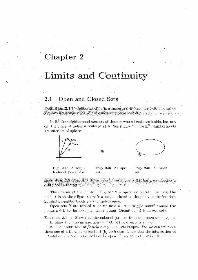
D efin itio n 2.1 (Neighborhood). Fix a vector a g R m and a S > 0. The set of x G IRm satisfying |x — a| < <5 is called a neighborhood of a. .

In R2 the neighborhood consists of those x whose heads are inside, but not on, the circle of radius S centered at a. See Figure 2.1. In R3 neighborhoods are interiors of spheres. .

Fig. 2.1: A neigh- Fig. 2.2: An open Fig.borhood: |x — a| < <5. set. set.

2.3: A closed

D efin itio n 2.2. A set U C R" is open if every point x £ U has a neighborhood contained in the set.

The interior of the ellipse in Figure 2.2 is open: no matter liovv close the point ® is to the ellipse, there is a neighborhood of the point in the interior. Similarly, neighborhoods are themselves open.

Open sets U are needed when we need a little “wiggle room” around th e points x G U to, for example, define a limit. Definition 3.1 is an example.

E x erc ise 2.1. a. Show that the union of (arbitrarily many) open sets is open.b. Show that the intersection n ()•> of I,wo open sets is open.c. The intersection of finitely many open sets is open. For we can intersect

them one a t a time, applying Part (b) each time. Show that the intersection of infinitely many open sets need not be open. There are examples in R.

14 ClIAPTBK 2: LIMITS AND CONTINUITY

Exercise 2.2. a. Let O be the set of x € R with a < x < b. Show that O is open in R. The set is called an open interval and denoted (a, b) , .

b. Let S be the set of (x , 0) e R2 with a < x < b. Show that S is not an open set in.R2.

D efin ition 2.3 (Complement). If A C B , then the complement B ~ A o i A m B consists; of those members of B not in A:

Definition 2.4. A set A C Rm is dosed if its complement in RTO is open.

The complement of the ellipse plus its interior in Figure 2.3 is open. Thus the ellipse plus its interior is closed. The ellipse itself is also closed.

E x e rc ise '2 .3. a. Let F j be the set of .t 6 R with a < x < b. Describe in words why Fi is a closed set in R. The set. is 'called a closed interval and denoted [a, b\ .

b. Let F 2 be the set of points in R2 with coordinates (.t,Q), a < x < b. Describe in words why F 2 is a closed set in R2..

E xercise 2.4. Is a single point in.R" open? Closed?

E xerc ise 2.5. Give an example of a set which is neither open nor closed.

Problem s 2.1

2.1.1. a. Is the empty set open? b. Is the empty set closed?

2.1.2. Let {Aq } be a family of sets, each A a being a subset of a set A. Denote the intersection of all A a by p)Q A a . This is similar to E notation for addition.

De Morgan’s laws state that ( f )a A a)' = Ua A!a ail(* ( U a -â)' = f l Q A!a , wheredenotes ‘‘complement in A ”. For example, ( j4a ) from the first law

consists of points not in all of the A a . And U A'tt consists of points not in at, least one of the A a . These sets are equal.

a. Show that the intersection of (arbitrarily many) closed sets Fa is closed.b. Show tha t the union Fi U F> of two closed sets is closed.c. P art (b) implies that tJie union of finitely many closed sets is closed.

Show that the union of infinitely many closed sets need not be closed. There are examples in R.

2.1.3. Show that every open set'. U in R" is a union of neighborhoods of pointsof U

S e c t i o n 2 .2 : L i m i t s 1 5

2.2 L im its

Limits are at the foundation of vector and geometric calculus, just as they are of scalar calculus. I will not give the technical definition of a limit. Instead, we will take as our starting point Theorem 2.6 below giving properties of limits.

We quickly review limits of scalar functions with two examples.

E x a m p le 1. The function f ( x ) = sh \x /x is not defined at x = 0 (the denominator is zero there). Figure 2.4 shows the graph of / . There is a “hole” in the graph at x = 0 which cannot be depicted. We see tha t even though. s in x / x is not defined at x = 0, if x approaches 0 (but is not equal to 0), then s in x / x approaches 1: iiinsinx/a; = 1.

F ig . 2 .4 : T he graph of s i n x / x . F ig . 2.5: A step function.There is no value at x = 0.

E x am p le 2. Figure 2.5 shows the graph of a step function:

f ( x ) =— 1, if x < 0;

1, if x > 0.

We see tha t as x approaches zero, f ( x ) does not get closer to a single value; lim/Or) does not exist. This is so whether or not / has a value a t 0, and if itI-i-0does, what the value is.

E x erc ise 2.6. a. Define f ( x ) = s in x /x for x ^ 0 and f i x ) = 2 for x = 0. Explain why limx_>o /(-t) exists.

b. Define f ( x ) = s in x /x for x < 0 and f ( x ) — 1 + x for x > 0. Does l im ^ o / ( 3;) exist? Explain.

sin (a;2 H- y~)E x erc ise 2.7. Docs lirn

(x,y)r>(0fi) • y-exist? Explain.

We can be a bit more precise-about the notion, of a limit. Let F: Rm —v Gn. Intuitively, lim /"’’(x) = L means that we can make jl'Xx) — L\ as small as we like,

X —> <1excep t . 0, if o n ly w e l a k e jx — aj s m a l l e n o u g h , hut n o t 0.

In particular, F (x ) must be delined if |x — a| is small enough, but perhaps not 0, i.e., i?(x) must be defined in some neighborhood of a, except perhaps at a. The value, or even the existence, of F(sl) is irrelevant to the existence of !imF(x).

16 C h a p t e r 2: L i mi t s a n d C o n t i n u i t y

Recall the norm of a multivector (LAGA Definition 6.10).

D efin ition 2.5 (Limit). Let F be defined on a neighborhood of a € Mm, exceptperhaps at a, and take values in Gn . Then lim F (x ) = L means that |F(rc) —L\

x—*acan be made as small as we want (except possibly 0) if |x — a| is small enough

' (but not 0).

The following theorem gives the fundamental properties of limits. There are many parts to the theorem. Parts (b)-(e) can be summarized by saying that limits behave well with respect to algebraic operations. Parts (a)-(g) generalize properties of limits of scalar functions.. We do not give proofs.

T h e o rem 2 S (Properties of limits).

a. Limits are unique: lim F(x) = L \ and lim F(x) = f,-2, then L\ L%.x - + a x —>a ■■■ '

Now let F, G : Km -> G". Then ' '

• b. lim (aF(x)) = a lim F (x ). • ■ ■x—j-a x—va

c. lim (F (x) + G(x)) = linrF(x) + lim G (x).Xj-J-a x—j-a x—>a

d. lim (F(x)G'(x)) ~ lim F (x ) lim Gfx).x—>a ■ x-->a . ■ x—>a

This also applies to the inner and outer products.

e. lim (F (x )/G (x )) = lim F (x )/l im G (x ).x—>a . x—>a : ■ ■ ■■x-*a- .

f. lim |F (x ) | = llim F (x)|.x~»a x—>a

g. If lim F ix ) exists, then |F (x ) | < M , a constant,x—

in some neighborhood of a, except perhaps a t a.

h. If f(x) e M'\ it has components which are also functions of x:

f(x) = ( / , (x), / 2(x), - •. , /«(x)).

Thenlim f(x) = ( lim f i ( x ) , lim / 2(x), . . . , lim / rt(x)).

X—>a • K -ii i -\ - - a ■ . . ■ x ->u •

Parts (b)-(f) are understood as follows. If the right side of the equation exists, then so does the left side, and the equality holds. In Part (e), we must also require that G(x) is invertible hi some neighborhood of a. If G(x) is vector valued, this .simply means that G(x) -r- 0 in some neighborhood of a.

Part (h ) asserts vliai the limit: on the left side exists if and only if all of those on the right do, and if the limits do exist, then equality holds.

E x erc ise 2.8. Suppose that limx_>a F (x ) = L and limx_>a G(x) = M . UseTheorem 2.0 to determine limx_ia(uF(x) + F(x)G (x)). State the parts of thei heorem i hat you u se .

S e c t i o n 2 .2 : L i m i t s 17

Problem s

2.2.1. The function sin(l/a;) .oscillates infinitely many times as x approaches 0.a. Describe in words why l im ^ o s in (l/x ) does not exist.b. Describe in words why l im ^ o £ sin(l/x') does exist.

2 2 •

2.2.2. Define / : R2 —> K by f ( x , y ) = ~ ( x , y ) ^ (0,0). Show th a tx y ■

Urn lira<. f ( x , y ) ± lira liin f (x ,y ) .x —>0 y— 0 y—>0 x-+0.

2.2.3. Define / : R2 —> R by f ( x , y ) = for (x,y) ^ (0,0). Show th a tx + y

lim f ( x , y ) does not. exist. Hint: Compute f { x ,y ) on the lines y = mx. >(o,o; • .

18 C h a p t e r 2: L i m i t s a n d C o n t i n u i t y

2.3 C o n tin u ity

D efin itio n 2.7 (Continuous function). Let F : U C Rm -» GM, where U is open. Then F is continuous a t si € U if lim F ix ) = F (a). And F is continuous

x —»a ,in U if it is continuous a t every a e U.

The existence of F (a) is irrelevant to the existence of lim F(x). But F(a)x—>a

must exist for F to be continuous at a.

The scalar function'sin(x)/a; is not defined a t ■ x = 0. Define a function

. ■ f t .\ _ f sm ( .x ) /x , . i f x ^ O ;^ ' 1 1 -I1 f\1 .1, it x — 0 .

Recall from Section 2,2 that lim s\n{x)/x ~ 1. Since /(0 ) = 1, / is continuousx—>0.

at x = 0. If instead we define /(0 ) = 0, then / is not continuous a t x = 0.There is no way to define the step function of Figure 2.5 at x = 0 so the

function becomes continuous there.

T h e o re m 2.8. Let F and G be defined on a neighborhood of a e Rm and take values in Gn. Let a be a scalar. Suppose that F and G are continuous at a. Then the functions in (a)-(e) are continuous at a.

a. aF.b. F + G.c. FG, F - G, F A G.d. F jG . Here G(x) must be invertible in some neighborhood of a.e. \F\.f. Let f : Rm —>■ Kn. Express f(x) in terms of components:

f(x ) = ( / i ( x ) , / 2( x ) , . . . , / n(x)).

Then f is continuous at a if and only if each /,■ is continuous at a.

Proof. All-parts of the theorem follow from properties of limits (Theorem 2.6). As an example, we prove Part (a):

lirn(aF)(x) = lim (aF(x)) = a lim F ix) = aF(a) = (aF)(a).x—7a x— x—

Steps (1) and (4) use the definition of aF. Step (2) uses Theorem 2.6b. Step (3) uses the continuity of F. □

E x erc ise 2.9. Prove Pari (b) of Theorem 2 . 8 .

Theorem 2> allows us to build continuous functions out of other continuous 1’uiictions.

E x erc ise 2.10. Suppose that functions F and G are continuous at x. Use Theorem 2.6 to show that aF + FG is continuous at x. State the parte of the

•theorem that you use.

S e c t i o n 2 . 3 : C o n t i n u i t y 19

T h e o r e m 2 . 9 (The composition of continuous functions is continuous). Let f be a continuous function at x e JR"1 with f(x) -- y e Rn. Let g be continuous a t y, Then g o f is cotitimious at x. V ■ '

We do not give a proof.

There is a second way to express continuity at a. It is a change of notation from our definition lim F(x) = F (a). Replace x with a + h in the definition.

X—»a - ,Then x —> a becomes a + h —> a, i.e., h —> 0. Thus F is continuous at a if and only if

lim F(a + h) = F (a). (2-1)h—>0 . •

T h e o re m 2.10. Linear transformations f are everywhere continuous.

Proof. We have lim f-(x + h) = lim (f(x) + f(h)) = f(x) + lim f(h).h—>0 h->0 h->0 .

We use the operator norm \f\o to finish (LAGA Problem 8,1.14). Since |f(h)| < |f|c>|h[,'Iimh->o |f(h) | = 0, so Eq. (2.1) is-satisfied. □

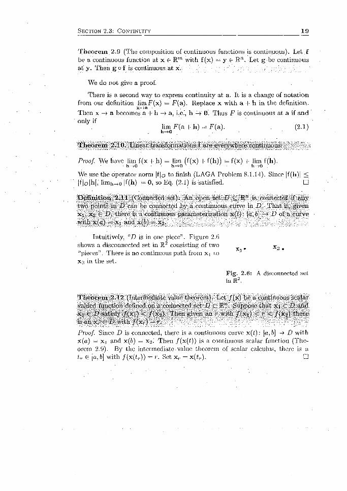
D e fin itio n 2.11 (Connected set). An open set, D C Rn is connected if any two points in D can be connectcd by a continuous curve in D. T hat is,.given x i, X2 6 D,. there is a continuous parameterization x(i): [a, 6] —» D of a .curve with x(a) = x i and x(6) = x 2.

Intuitively, “D is in one piece” . Figure 2.6 shows a disconnected set in K2 consisting of two X2“pieces” . There is no continuous path from x j to Xl x 2 in the set.

F ig . 2.6: A disconnected se t in R2.

T h e o re m 2.12 (Intermediate value theorem). Let / (x ) be a continuous scalar valued function defined on a connected set D c f i71. Suppose tha t xj £ D and xa € D satisfy / ( x t ) < / ( x 2). Then given an r with / ( x t ) < r < / ( x 2) there is an x r e D with / ( x r) = r.

Proof Since D is connected, there is a continuous curve x(/;): [a, b] D with x(a) = Xi and x(6) = x 2.' Then /(x ( i) ) is a continuous scalar function (Theorem 2.9). By the intermediate value theorem of scalar calculus, there is a t r G [a, b] with / ( x ( i r)) = r. Set x r = x ( tr ). □

2 0 C h a p t e r 2: L i mi t s a n d C o n t i n u i t y

Problem s 2.3

2.3.1. Prove Part (f) of Theorem 2.8.

2.3.2. Assume that polynomials and trigonometric functions are continuous. (They are.) Show that (x2y 3 + x 3y 2 4- s in x )/(x 2 + y 2 + 1) is continuous.

2.3.3. Find a value of c so that this function is continuous:

n \ i x + c> if x ^ 3; f ( x ) = 1 i e' , lx~, i f :c > 3 .

2.3.4. Let f : U C R"‘ -»• Rn, where V is an open.connected set, be continuous. Show that the range of f is connected.

Part II

Derivatives

Chapter 3

The Differential

The derivative f ' of scalar calculus plays two roles: it gives us tangent lines to the graph of / and rates of change of /.■ In higher dimensions the two roles are played by different derivatives. They are the topics of two chapters of P artII of this text. The diffei'ential (Section 3.3) gives us tangents. The gradient (Section 5.2) gives us rates of change. Both derivatives are fundamental.'

3.1 T h e P a r t ia l D eriva tive

D efin itio n 3.1 (Partial derivative). Let F: U C E m —)• Gn , where U is open.Let x € U have coordinates (a:i,£2 ,— , x m) with respect to an orthonormal basis {<•.]. e-2 , . . . ,e m}. Then the partial derivative of F with respect to is

S F(x) F (x -f heA - F (x)- „ — = hm • —---- , ----- — .

O X i h - t o h

We will often abbreviate this to dtF.

The partial derivatives also map U to Gn. In terms of coordinates,

d F (x ) _ F ( x i , x 2, X i + x m) - F ( x i , x 2, . . . , x i t . . . , x m)

dXi ~ h

We see that dF(x) /d x i is the ordinary derivative of F with respect to i;., with the other x ’s fixed. In other words, the other a;’s are treated as constants. Thus computing partial derivatives requires no new skills. For example, if / : -> K is defined by f ( x , y, z) = zexy, then d f / d z = exy and d f / d x = yzexy.

E x erc ise 3.1. Define f : R2 -7 R2.by f(.ri +. j/jj = x 2yH 4- xj. Compute d f / d xand d i /d y . (Since R" C O", a function mapping /•,’/•"' in ]Rn qualifies as an F in Definition 3.1.)

E x erc ise 3.2. Let f ( x , y) = -------.— — ----- Compute d f / d x with SymPy..7; sin (;y sin(.'r‘;osw ))

2 4 C h a p t e r 3: T h e D i f f e r e n t i a l

The words “partial derivative” are often abbreviated to “partial” , as in “the partial of- F with respect to .

T h e o re m 3.2 (Partial derivative properties). Let J -1 and exist at x. Then the right sides below exist at x and are equal to the left sides at x.

D(aF) 8 F

a- d x l ' ~ a dx.i

b ^ (F + G) OF 8 Gdxi ■ dxi "I" dxi

d ( F G ) _ dG . OF c- — <\ — r ^-----r ■ Cr-

OXi OXi OXid l F - G ) d (F A G)

Similar rules apply to -— ..... .. a n d ---- - — ..• “ OXi • (>x.i

Be careful of the order-here, as; multivectors do not in general commute.

Proof. The partial derivative is performed component by component on the scalar coefficients of F. The.partial derivative of each scalar coefficient is performed witli the variables other than Xi held constant. Thus satisfies the analogous rules from scalar calculus. □

When / is given explicitly as a function of scalar variables, e.g., f ( x , y ), then we often write, e.g., d f / d x = f x .

E x erc ise 3.3. Let f { x , y ) = for (x ,y) ^ (0,0) and let /(0,Q ) = 0 . -a. Show tha t f x(0,0) and f y (0,0) exist. Since /(0 ,0 ) is defined specially,

SyrnPy cannot compute f x (0,0). You must compute it from its definition.b. Show th a t f is discontinuous at (0,0). Hint: Approach (0,0) along the

line y = x.

The exercise shows tha t the existence of all partial derivatives of a function is a rather weak condition. This is no surprise: the existence of partial derivatives tells us nothing about the function off of the coordinate axes. In Section 3.3 we will meet the stronger condition of differentiability of a function.

S e c t i o n 3 .1 : T he P a r t i a l D e r i v a t i v e 2 5

M ixed Partia l D erivatives

A function F (x , y) has four second order partial derivatives:

d2F d 2F (PF d 2F '

d x2 ’ d y d x ’ d x d y ? ■ dy2 ’

d2F d ( 8F \where, for example, ——— = ~ . The derivatives are taken right to left.

d y d x ay \ d x J

E x erc ise 3.4. a. Compute the four second partial derivatives of f ( x , y ) = yex .b. Compare d 2f / d y d x and d 2f / d x d y . .

T h eo rem : 3i3 (Mbced partials a.re equa,l). Let F be defined in an open .set in R ”\ Suppose that the second partial derivatives of F are continuous in'-27. Then for x £ U and i ^ j , Q ip g i p

dxidx j d x jd x i ■

The derivatives are called mixed pariials.

This theorem will be invoked many times in this book.

Proof. It suffices to prove the theorem for scalar • valued / , and apply the result to each component of.if . For ease' of notation we,prove the theorem for f ( x , y ) . Define

S (h ) = ( f ( a + h, b + h) - f ( a + li, b)) - ( / ( a , b + h) - f ( a , b))

and A ( x , y ) = f ( x , y ) — f ( x . b ) . Then using the scalar mean value theorem (Problem 3.1.2) in Steps (2) and (4),

S (h ) = A (a + h ,b + h ) - A (a , b + li) = b + h)

h ( ^ b+k) ~ f x ^ b)) 4

where £ is between a and a 4* h and r; is between b and b + h.

d~fTherefore, using the continuity of ... . at (a, b),

a y a x

, S(h) d2f , r , I f f , „Inn — — = lim (£,?;) = ,, » («,»)•h-»o hr h ~ o d y d x d y d x

Similarly (Exercise 3.5),

..s ( h ) .... a 2/(a. If). (3.1)

h-ro h- d x dy

The la*t two equations establish the theorem. □

E x e r c is e 3 .5 . Prove Eq. (3.1). Hint: Define B ( x , y ) = f ( x , y ) — f ( a , y ) . Then S (h ) = B (a + h, b + h) - B ( a + b).


E xercise 3.6. Show that the mixed partials. of / (x , y) = sin(x2y) are equal.

E xercise 3.7. Therrnody narri ics teaches that the energy E of a rigid container of gas is a function of its entropy S and volume V : E = E (S ,V ) , Its temperature is given by T = d E / d S and its pressure by P = —d E /d V . Show tha t d T / d V — —dP/dS.' This is a Maxwell relation.

The relation is usually written (d T jd V )s = . —{8 P / d S ) v in physics and chemistry texts to make it dear that S is held constant on the left and V is held constant on the right when computing the partial derivatives.

The existence of mixed partials does not guarantee their equality. Here is an example. •

„ , / a S £ p A *<*,'<*. . - . f( x>y) = < x 2 + y--U if (* ,» ) = (0 , 0).

We show that 0) 7 f y r ( 0 , 0)- Since / ( 0 ,0 ) is defined specially, Sym Py cannot compute f x (0 ,0 ) . We compute it from its definition. Since /( :r .0 ) = 0 for all x,

0. ■/*->o h

By hand or from SyrnPy, for (x, y) / (0 ,0),

j/(x4 - ? / + A i r y 2)- ■

In both cases, /* (0 ,y ) = —y. Thus

, ^ ■UQ.O + h) - / T(0.0) - h - 0L v ( 0 . 0 = lim JxK— ^ = llm ---- -----

v v ' h-+a h h-io h,

Note the order of differentiation f xy = ( f x )v .

Exercise 3.8. Show that /„*((), 0) = 1. Thus the mixed partials are not equal.

S e c t i o n 3 .1 : T h e P a r t i a l D e r i v a t i v e 2 7

P roblem s 3.1

v + w = z —;y.

F ig . 3.1: The mean value theorem.

3.1..1. Let it, v, w be functions of a;, y, z:

u — v + 2w = x + 2z, 2u + v — 2w = 2x — 2z,

Find du/dy , d v fd y , dw/dy.3.1.2 (Scalar mean value theorem). Figure 3.1 illustrates the mean value theorem of scalar calculus. The chord between (1 ,/(1 )) and (2,/(2),) is shown. Visually, there is a c, 1 < c < 2 where the tangent line to the graph is parallel to the chord. This tangent line is also shown.

T h e o re m (Scalar mean value theorem). Let / be continuous on the closed interval [a, b] and differentiable on the open interval (a,b). Then there is at least one point

c € (a ,b) where / '(c ) = i-e., the slope of thetangent, line is equal to that of the chord. This is an existence theorem: it tells us that a c exists, but does not tell us how to find it.

The figure shows the graph of f ( x ) = 2a;3 -- 4a:2 + 3.a. Find the slope of the chord.b. Find the c of the scalar mean value theorem.

We will extend the mean value theorem to scalar valued functions of a vector variable in Problem 3.4.13.

3.1.3. Show that the mean value theorem does not hold for functions f : R —> M". Use the curve f (t) = cosii + sin fj, 0 < t < 2tr.

3.1.4. If z = f ( x \ , x 2, ■ ■ ■ , x n) is a real valued function, then Eli(z) = is called the elasticity of z with respect to Xj.

a. Show that Eli(yz) = El{(y) + Eli(z). If a is a constant, then clearly Eli(a) = 0. Thus Eli(az) = Eli(z).

b. Replace Xi by ax;. Show that Eli(z) is unchanged. Hint: Use the scalarchain rule for a suitable w.

c. Suppose tha t Xi changes by a small amount Aa;*, causing a small changeA ; / "-/ x . i the percentage change in z divided by th eA z . Show that El{(z) s

percentage change in x ^Parts (a) and (b) show that, unlike the partial derivative the elasticity

Eli(z) is unchanged by a change of units of z (z az) or (a;,; —> ax j ) . Part (c) shows that, for example, if E k (z ) = 2, then a 1.5% increase in x,i will cause approximately a 3% increase in z. These properties of elasticity make it useful in a wide variety of applied disciplines. For example “the elasticity of [taxij trip demand with respect to feres is estimated to bo —0.22.” 1 You need not be an economist to understand why this number is negative.

1I3. Sclialler, E las t ic i t ie s f o r taxicab fa re s a n d se rv ice availability, T ra n s p o r ta t io n 2 6 283- 297 (1999).

28 C h a p t e r 3: T h e D i f f e r e n t i a l

3.2 T h e Taylor E x p an sio n

Recall the summation convention, where a repeated index is summed over, without, use of a £ (Page 4). •

Taylor expansions of scalar functions generalize to scalar valued functions defined on Kn . In fact, we will see that the vector version is a corollary of the scalar version using a clever trick. As in the scalar case, Taylor expansions allow us to approximate functions with polynomials. •

T h e o re m 3.4 (First order Taylor expansion). Let / .h e a scalar valued function defined on a ball B C Rn centered a t x and with continuous second order partial derivatives there. Abbreviate = djdj. Then for x + h € B,

/ ( x + h) = / ( x ) + d j f ( x ) h i + 1 3 i j /(x + t*h)hihj, (3.2)

for some t*, 0 < t* < 1. The sums on the right run from 1. to n.

Proof.. Define the scalar function g(t) = / ( x + th) (the trick). One form of the first order Taylor expansion of g(t) at t = 0 from scalar calculus is

g ( t ) = y ( Q ) + g ,(0)t + ^g,' ( t* ) t \ . (3.3)

for some t*, 0 < t* < 1 .Now pause the proof for a little exercise.

E xercise 3.9. Show tha t g'{t) = /'../(x : In particular, g'( 0) = i>, f .

Take another derivative: g"{t) = d i j f ( x + th )h ih j . Substitute g'(0) and g"ii*) into Eq. (3.3) and set t — 1 to obtain Eq. (3.2). □

In the next two exercises the word “approximate” means use Eq. (3.2) with the last term on the right omitted. The error made is this last term. Problem 3.2.3 puts a bound on the error.

E xercise 3.10. Approximate f ( x , y ) = 4/ ( x + y) near (x,y) = (1,1). Your answer should be of the form / ( I + hi, 1 + ho) « a + bliy + cli2 , where a, b, c are constants.

Exercise 3.11. Let f ( x , y ) = x y x.a. Approximate /(1.01,2.02).b. Multiply out /(1 .0 1 ,2.02) = (1 + .01)(2 + .02)2. Show tha t the terms left

out of the approximation of Part (a) are products of at least two small terms. Show that the error in the approximation is .03%.

Apply Eq. (3.2) to cad i com ponen t of a vector valued f (x ) to ob ta in the ■approximation

f(x + h) « f(x) + dii(x)lii. (3.4)

Tlie term <)lf(x)/tj, which allows us to approximate f near x linearly, is at the (XJitcr of this Part II of the, book. We will look at it in several ways, starting in the next section.

S e c t i o n 3 . 2 : T h e T a y l o r E x p a n s i o n 29

There is also a second order Taylor expansion. If / has continuous third order partial derivatives, then

/ ( x + h) = / (x ) + d i f (x)h i + \ d i j f (x)hihj + ±dijkf ( x + t*h)hihjhk , (3.5)

for some t * ,0 < t* < 1. This is proved in a similar manner to Theorem 3.4.

E xerc ise 3.12. Let f ( x , y ) = 2 + 3x2 + Axy + ex + y3. Approximate / near (0,0) using Eq.(3.5) without the last term on the right.

There are Taylor expansions of every order, as long as we can continue to take partial derivatives. Using all orders we can form an infinite series. An infinite Taylor series of a scalar function f ( x ) centered at x usually converges to the function in an interval, perhaps infinite, centered at x. Similarly, an infinite Taylor series of a vector valued function / ( x ) centered at x usually converges to the function in a ball centered a t x. We will not consider these matters.

Problem s 3.2

3.2.1. Approximate f ( x , y ) = e1 cos y near (x, y) = (0,0) with the first two terms on the right side of Eq. (3.2).

3.2.2. Approximate sin(7r/6 + .01)cos(7r/3 + .02) with the first two terms on the right side of Eq. (3.2). Notice tha t you make the same calculation in Exercise 3.24.

3.2.3. a. A p p ro x im a te /(x + h ) with / (x ) + d i f (x )h i from Eq. (3.2). Then the error E is the omitted rightmost term. Show that

\E\ < + < < ^ | h | 2,

where M is the maximum of |d y / ( x + i*h)| over all i , j and 0 < t* < 1.The importance of this bound on E is that if the hi are small, then so is |h |,

and |h |2 is smaller still.b. Put a bound on E in Problem 3.2.1 for |(a;,y)| < .01. Fact: e L01 < 3.

3 0 C h a p t e r 3: 'L'h e D i f f e r e n t i a l

3.3 T h e D ifferential

Let f : U C Rm —>• R", • where U is open. Suppose that all d f /d x j exist at x € U: For h = hiCi 6 Rm (summation convention used) consider the expression hiditix ) from Eq. (3.4). Fix x and think of it as a function of h. Denote it f£:

£ (h ) = M if (x ) . (3.6)

E xerc ise -3.1-3. Show tha t f*: U Q Rm —> R" is a linear transformation.

Actually, we are not entitled to use the notation unless the condition in the following definition is met. .

D efin ition 3.5 (Differentiable function, differential). Let f : U C Rm R". where U is open. Fix x € U . Define r(h ) by

f(x -f h) = f(x) T f^(h) + r(h ). (3.7)

(The equation does define r(h ), as the o tl® :term s are known.) If

(3 ’8)

then the linear transformation : R™ R n is called the differential of f at x,and f is said to be differentiable at x.

If f is differentiable at x, then f (x) is approx im ate near x by a very simple kind of function, a constant plus a linear transformation:

f(x + h) « f(x) + f '(h ) ,

with an error r(h ) satisfying Eq. (3.8). Therein lies the importance of the differentiability of a vector function.

In general there is a different linear transformation for each x, as the notation indicates. The simple functions in the next three exercises are exceptions.

E xerc ise 3.1,4. Let f(x) = x.. Show that f£(h) = h; the differential of the identity function is the identity linear transformation. Hint: Write x = xjGj.

E x erc ise 3.15. Suppose f(x) = a, a constant vector. Show that = 0; the differential of a constant function is the zero linear transformation.

E x erc ise 3.16. Let f be a linear transformation. Show th a t f* = f: the differential of ;'i line<.ir I l’ans lonnaf ion is t h a t linear i r ans ionua t ion .

A function can have all partial derivatives at a point without being continuous there (Exercise 3.3). The next exercise shows tha t a differentiable function is continuous. You may remember the analogous theorem of scalar calculus.

E xerc ise 3.17. Definition 3.5 requires not only that r(h) —> 0, but the strongerr(h )/ jh | ..> (!. Show that r!h) 0 states that f is continuous at x.

S e c t i o n 3 .3 : T h e D i f f e r e n t i a l 3 1

The next exercise shows that, despite appearances, the differential f£. of vector functions is a generalization of the scalar derivative f ' ( x ) of scalar calculus.

E x erc ise 3.18. Suppose that f {x ) is a scalar function and f ' ( x ) exists. Define 7’(/i) by

f ( x + h ) = f ( x ) + f ' ( x ) h + r(h). ' (3.9)

■ Show tha t lin i/ô r (h ) /h — 0.For a fixed x, the mapping h m- f '{ x )h is a linear transformation of h on R,

so the scalar derivative f ' ( x ) is the differential of / at x.

Differentiability is the condition we need to obtain the key theorems of this chapter: Theorems 3.10 and 3.14. But it is usually difficult to verify differentiability using Definition 3.5. Theorem 3.6 provides a simple criterion which suffices in most cases.

T h e o re m 3.6. Let f : U C Rm R71, where U is open. Suppose that all d j i ( x ) /d x j exist in some neighborhood of x € 17 and are continuous at x. Then

exists, i.e., f is differentiable at x.

Proof. We first prove Eq. (3.7) for each component / = f i of f. Set xo = x and

Xfc = x 0 + Y l j= i Then

n rt ' n/ ( x + h) - /(x ) - '}Tdkf(x.)hk =. ]T /( / (x fc) - / ( x fc_i)) - ^2 dkf(x)hk

k=1 k= 1 k=\ j n

= {9kf(x.l)hk - dkf(x)hk) (3.10)I k = 1

^ lh l I <9fc/ ( x ;) - ^ - / (x)|- fc=l

The first sura on the right side of Step (1) is a telescoping sum: all terms cancel except / ( x n ) = / ( x + h) and —/( x o ) = —/ ( x ) . Write out the sum to see this. Step (2) applies the scalar mean value theorem (Problem 3.1.2), with x£ on the line segm ent between x^_i and x fc = x fc_j + /ifcefc. (Thus x£ = x ^ - i + 0khke/c for some Ok G [0, 1].) Step (3) uses the triangle inequality and |/it| < |h|.

Now divide the right side o f Eq. (3.10) by ]h| and let l n O . By the continuity of the partial derivatives the result approaches (3 if each x£ —» x. To see this:

\Xkk - l k

T , h j e j + O k h k e k < ^ \h j \ < n j h j ,

i j =i

We now have for each f i a scalar equation with a scalar r,-(h) like Eq. (3.7). Multiply the equation for f i by e; and add, giving Eq. (3.7) with r(h) = r;(h )e7;. Then by the triangle inequality limiw o lr (h)|/|h | < limiw o |ri(h)|/|h | = 0 . □

D efin itio n 3.7 (Continuously differentiable). If f(x) lias continuous partial derivatives in a open-set U C Rm. then f is continuously differentiable in U.

From Theorem 3.6, if f is continuously differentiable in U, then f is differentiable throughout IJ. (Confusing terminology, but it is standard. Remember: “f is differentiable in U" means “f£ exists for x £ U”.)


T h eo rem 3.8 '(Differential properties). Let a be a scalar and f and g be differentiable vector valued functions defined on an open set U C I n . Then

a. (af)x — af£. b- (f + g)x ~ C + gx-

These follow from Theorem 3,2.

T h eo re m 3.9. Let f : Rm —> R ” be differentiable at x. Then, the matrix of the linear transformation f ' is

r d f i d h d f i 1dx \ dx'2 dxm

d h Oh ' d h ■dx\ 8x2 ()j-m

d h Of 11 8 f n-dxi Ox 2 . ■ . 8xm .

(3.11)

evaluated a t x. 'This n x rn matrix is called the Jacobian matrix of f .

Proof. Substitute h = e., in Eq. (3.6): f*(ei) = Sjf(x). Then Eq. (3.11) is the matrix representation of the differential (LAGA Theorem 9.1). □

When m — n the determinant det[f£] is called the Jacobian determinant off . It is often denoted

det-[f'] =d ( f l j 2, . - - j r n )

d ( x i , x 2(3.12)

Most often the Jacobian determinant is simply called the Jacobian, but sometimes the Jacobian matrix is called tha t as well.

E xercise 3.19. Define f : R2 ->• R2 by f ( x \ , x 2) = (a:2, ,Ti + X2 ). Determine the matrix [f'T ?/)],

E x erc ise 3.20. a. Let f (x ,y , z) = (x 2z , x + y + z). Compute [f(-a. 2j],

I). Using Part (a), compute [f^ [h] in terms of the components of h.

E xerc ise 3.21. Let f (x ,y , z ) — (x2 cos(y), ^rzyi, -z log(sin(:z:))).' Compute

|ffr ,,-)]• Use SymPy. , .

E xerc ise 3.22. Lei, f : II" —> K" be differentiable at x. When will jf^j be a diagonal matrix?

If f : E m —:> ]Rr" is differentiable a t x, then the outennorphism extension of f ' satisfies f£(l) = det (f^)I (LAGA Eq. (S.1‘?)). This gives a formula for the .Jacobian determinant of f not involving partial derivatives: del (f^j (i ; *.

S e c t i o n 3 . 3 : T h e D i f f e r e n t i a l 3 3

Problem s 3.3

3.3.1. Let f(x) be a vector valued function of a scalar x. Show that f'(x) =

lim/t_x) exists if and only if the differential ¥x exists.f (x + h) — f (x)h

3.3.2. Define f ( x ,y , z ) — (z + x2siny , z ( x 3 + y2)). Compute [f^ y>2)]-

3.3.3. Determine the differential of the spherical coordinate transformation {p,Q,4>) -*• (x , y , z ) (Eq. (1.10)). Use SymPy.

3.3.4. Let / ( x ) — x 2. Show that / x (h) = 2x • h.

3.3.5. Let f be a linear transformation and define g(x) = f (x) • x. Show th a t fi4(h ) = f(x) - h + f(h) • x.

If f is symmetric, then f(h) • x = h - f(x), so <?x(h) = 2f(x) • h.

3.3.6. Suppose tha t f(x) ^ 0 and that and ( l / f ) x exist. Prove the formula

3.3.7. This problem shows that the converse to Theorem 3.6 is false: the existence of f* does not imply that f is continuously differentiable at x.

a. Show that d f (0 ,0 ) /d x = 0. Similarly, d f (0 ,0 ) /d y = 0.

b. Show that d f / d x is discontinuous at (0 ,0 ) ,

c. Show that / is differentiable at (0 , 0 ) with / | 0 0)(h) = 0 for all h, i.e.,

/ ( o, 0) is the zero linear transformation.

Hint: (1 / f ) f = 1. If 1 /f and f^ commute (for example if f is scalar valued),

then the right side becomes — as hi scalar calculus.

Let

3 4 C h a p t e r 3: T he D i f f e r e n t i a l

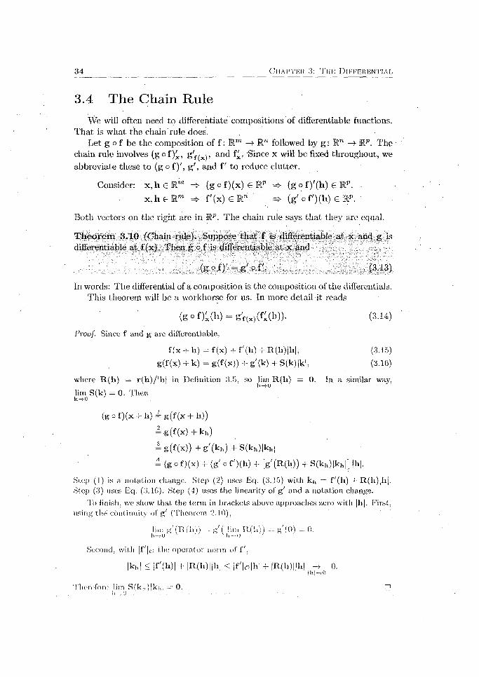
3.4 T h e C h a in R u le

We will often need to differentiate compositions'of differentiable functions. That is what the chain rule does.

Let g o f be the composition of f : E m —> R” followed by g: Rn —> Mp. The chain rule involves (g o f)^, g f(x)> and fx- Since x will be fixed throughout, we abbreviate these to (g o f )', g ', and f ' to reduce clutter.

-Consider: x, h e Km =!> (g o f)(x) 6 Kp => (g o f) '(h ) € IRP. .

x, h e Mm => f ' ( x ) e r => ( g ' o f ' X h J e r .

Both vectors on the right are in Rp. The chain rule says that they are equal.

T h e o re m 3.10 (Chain rule). Suppose th a t f is differentiable at x and g is differentiable at f(x). Then g o f is differentiable at x and

(g O f)' = • g' O f'. ' (3.13)

In words: The differential of a composition is the composition of the differentials. This theorem will be a workhorse for us. In more detail it reads

( g o f ) x ( h ) = g f (x)( £ ( h ) ) . (3.14)

Proof. Since f and g are differentiable,

f ( x + h) = f (x) + f'(li) -I- R (h )] l i | . (3.15)

g ( f (x ) + k) = g ( f (x ) ) + g'(k) + S (k ) |k |. (3.16)

where R (h ) = r (h ) / |h | in Definition 3.5, so ]irn R (li) = 0. In a similar way,

lim S(k) = 0. 'Chen k->0

( g ° f ) ( x + h) = g ( f ( x + h ) )

— g ( f ( x ) + k h)

= g ( f ( * ) ) + g ' ( k h) + S (k h ) |k i , |

= ( g ° f ) ( x ) + ( g ' o f ' ) ( h ) + [g ' (R (h )) + S ( k h)|kh|] |h|.

Step (I) is a notation change. Step (2) uses Eq. (3.15) with kh = f ' (h ) + R (h ) |h | . Step (3) uses Eq. (3 .IG). S(,ep (4) uses the linearity o f g ' and a notation change.

To finish, we show that the term in brackets above approaches zero with |h|. First, using the continuity of g (Theorem 2.10),

lim fii'flUb'i) - «'( lim llfh)} = g'fO) - 0.' I) ,o ' '

S e c o n d , w i t h | f r |ci t h e o p e r a t o r n o r m o f f ' ,

|k h | < |f'(li) | + |R (h ) | |h | < - | f ' |o |h | + |R (h ) | | l i | 0.

T h e r e f o r e l im S ( k | , ) j k [ , | 0 . □

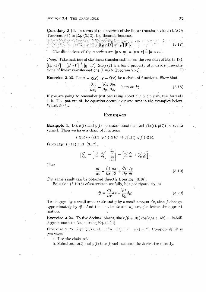
S e c t i o n 3 .4 : T h e C h a i n R u l e 3 5

C o ro lla ry 3.11. In terms of the matrices of the linear transformations (LAGA Theorem 9.1) in Eq. (3.13), the theorem becomes

' [ (g o f) /]= [g '] [ f '] . (3.17)

The dimensions of the matrices are [p x m\ = \p x n] x [n x m].

Proof. Take matrices of the linear transformations on the two sides of Eq. (3.13):

[(g of) '] = [g' o f'] = [g'j [f']_ Step (2) is a basic property of matrix representations of linear transformations (LAGA Theorem 9.2c). □

E xerc ise 3.23. Let z = g(y), y = f(x) be a chain of functions. Show that

' dzi dzi dyk

<"“ **>• <31S)If you are going to remember just one thing about the chain rule, this formula is it. The pattern of the equation occurs over and over in the examples below. Watch for it. . . .

Exam ples

E x am p le 1. Let x(t) and y(t) be scalar functions and f (x ( t ) ,y ( t ) ) be scalar valued. Then we have a chain of functions

t <E M i—}■ (x(£), y(£)) <E M2 i—}■ j (,%■(£), y(£)) <E M.

From Eqs. (3.11) and (3.17),

dxr<M_] = \9£ 0/1 dt _ \m d x + aidy\ i d t \ dy J ciy |_dx dt dy dl J

Thus

dt

df_ = df_dx df_dy

dt d x dt dy d t ' { ' 1

The same result can be obtained directly from Eq. (3.18).Equation (3.19) is often written usefully, but not rigorously, as

d f = Wxd X + % dy:' (3-20)

if rr changes bv a small amount dx and y by a small amount dy, then / changes approximately by df. And the smaller dx and dy are, the better the approximation.

E x erc ise 3.24. To five decimal places, siii(/r/6 + .01)cos(7r/3 + .02) = .24545. Approximate the value using Eq. (3.20).

E x erc ise 3.25. Define f ( x , y) = x 2y, x(t) = f:i, ;/(/.) = t2. Compute df j dt in two ways:

a. Use the chain rule.b. Substitute x(t) and y(t.) into / and compute the derivative directly.

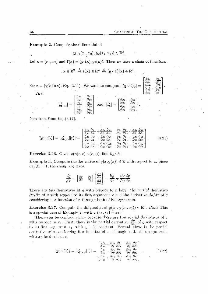
3 6 C h a p t e r 3: T he D i f f e r e n t i a l

E x am p le 2. Compute the differential of

E (y i (x i ,x 2), y2{xi ,X2)) e M 3. , '

Let x = (£ 1, 2:2 ) and f(x) = (?/i(x),t/2 (x ))- Then we have a chain of functions

. x € R2 A f (x) € R2 A (g o f)(x) e R3.

Set z = .(g '° f)(x), Eq. (I

First

' (gf(x)] =

Now from from Eq. (3.1

We want to. compute [(g o f) .] =

" d z \ d z 1d y i d y 2dz-2 dz?d y \ dy-2dz-s dz-j

. d y 1 dy-2

and [4]d y 1 Qy\dx\ dX2dy-2 dy2dx'i ■ 8x2

d z \ d z \

i i8x2dZ2

d x 1d z \

dx-2dzu

d x 1 dx-2

d z \ d y \ | dz-j d y 2 d y \ d x \ dy-2 d x \Szo d y 1 1 Bz-2 dy-2 ■ By\ d x \ dyo dx^

d z i d y 1 , dz \ 0y2 ' d y \ d x 2 dy? d x i dz'> dy\ dz-2 dy-2-

[(gof)x] = [gr(x)]K] =dz:j dy i _j_ d z 3 dt/2 _______ ______

d y \ d x 2 dy2 ’dx'±_

E xerc ise 3.26. Given g(u(r, $),v(r, .$)), find dg/dr.

dy\-dx% dy-2 dxodz-.j d y i . dz.i d y i “T ;

(3.21)

E x am p le 3. Compute the derivative of g(x, y(x)) e R with respect to x. Since dx /dx = 1, the chain rule gives

dg_dx

\diL dad y

"dxd xd yd x _

9gdx

dg dy

hi

There are two derivatives of g with respect to x here: the partial derivative d g /d x of g with respect to its first argument x and the derivative dg/dx of g considering it a function of x through both of its arguments.

E x erc ise 3.27. Compute the differential of g(.x'i, y(x 1, 0:2 )) € M'1. Hint: This is a special case of Example 2, with y i ( x i ,X 2) = X \ .

There can be confusion here because there are two partial derivatives of g with respect to Xi. First, there is the partial d e r i v a t i v e - o f g with respect •to its first argument .cj, with y held constant. Second, there is the partial derivative of g considering it a function'ol ./■] through both of its arguments, with x-> held constant.

Qsl j_ l)z 1 Jhtd y i Dy Ox 1Sz-2 | Dz_2 dy S y i d y d x 1rh:>

u dy1d?:j. .$21

d.r I

Dzi dy d y d x -2dz-2 dy d y d x 2 d d ydy dx->

S e c t i o n 3 . 4 : T h e C ha in R u l e 3 7

T h e o re m 3.12 (Differential of an inverse). Suppose that f : K." —> Rn is continuously differentiable in an open set containing a and. that the linear transformation is invertible. Then the inverse function (f /J^ 1 is differentiable a t f(a ) and ( f “ % a) = ( Q ~ l -

In words: the differential of an inverse is the inverse of the differential.

Some details were left out of the statement of the theorem. First, because f is continuously differentiable, exists (Theorem 3.6). Then f -1 exists and is continuously differentiable in some open set containing f(a) (Theorem 3.17, the Inverse Function Theorem). Thus (f_1)f(x) exists in an open set containing

f(a) (Theorem 3.6 again).Problem 3.4.8 asks you to prove the theorem.

E x erc ise 3.28. Let (r,6) be the polar coordinates of a point (Eq. (1.8)). Then its cartesian coordinates are (x , y ) = f(r, 0) = (rcos6, r sin#),

a. Compute [f . and determine when it is invertible,

b; Compute [(f-1 ) ^ y)] using Theorem 3.12. Then write [(f-1 ) ^ y)] in terms of x and y.

Problem s 3.4

3.4.1. Define f : R3 —> R3 by f(x, y, z ) = (xy ,y z , zx ) and g: R 3 —> R by g(u ,v ,w) = uvw. Using the chain rule, compute j(<7° f)'].

3.4.2. Let f ( u ,v ) = uv2 + v \ u = x 2 + y 2,v — 2y,x — t2, and y = 'M + 1. Express the matrix [df /dt) as a product of three matrices using the chain rule.

3.4.3. Let / : Rm —> R and suppose that exists. Show tha t (Z11)* exists for n £ 0 and that ( / " ) ; = n / ” - 1^ ) / ^ .

3.4.4. Let f be a function from Rm to R" and g a linear transformation from R” to Rp. Show tha t (go f)x(h) = g(f4(h)).

3.4.5. Let u(x, t) = f ( x — vt) + g{x + v t ), where / and g are scalar valued.

, t') t'jShow that v 2— „ ’ - = .. — . This is a partial differential equation. It is

o x 2 o tcalled the wave equation. Most laws of physics are expressed as partial differential equations.

Hint: (x, t) M- x — vt f i x — vt) is a chain of functions R2 —> R —> R.

3.4.6. Suppose tha t f ( x , y ) is homogeneous of degree n: f ( t x , t y ) = tnf ( x, y),

where « =?£ 0 is fixed. Show that x — + y —; = nf ( x . y).

3.4.7. Use the chain rule to expand ( h o g o f ) ^ . Hint: h o g o f = h o ( g o f ) .

3 .4.8. Prove Theorem 3.12. Hint: See Exercise 3.35 and note that x can be written i(x), where i is the identity linear transformation.


3.4.9. Define f : K2 —> R2 by f(x-, y) = (ex cosy, ex siily).

a - Find f(0,ff/4)' 'b. Note th a t f(0,7r/4) = (y/2/2, \/2 /2 ); F ind,f-1 '(v^ /2i>/2/2).

c. Approximate f ~ l ( \/2 f2 + ,01 ,\/2 /2 + .02) without computing f -1 . Use Eq. (3.7) without the small r(h ) term.

d. Apply f to your answer to Part (c) to see if it is reasonable.

/ -r 4- y \ Q z ( ) z3.4.10. Let z = f I ------- ), x ^ y. Show that x —— h w— = 0. Relate this to

\ x - y j ‘ d x ' d ythe result of Problem 8.4.6.

3.4.11. For x > y and u > v the .functions (u,v) — (e* + e2/,e:r — ey) and (x,y) — ( in |-(« + t ’),ln £(u — w)) are inverses. Compute the matrices of their differentials (Jacobian matrices), Eq. (3.11), and show that they are inverses, as stated by Theorem 3.1.2. ■ ,

3.4.12. Suppose that f ( x , y, z ) is continuously differentiable in a neighborhood of (z0,2/oi ô) and th a t none of §£ ,§£ , §{- is zero at {x0,y 0, z0).

Problem 3.6.7 asks you to show that f ( x , y , z ) = 0 defines functions x = x{y ,z) , y = y(x ,z ) , and z = z (x ,y ) in neighborhoods of (yo,z0), (xq, zo), and (xQ.yo) respectively. The partial derivatives in this problem are partial

derivatives of these functions. For example, dx d y

a. bhow that —— — = 1.ay ox 3 t f)n '() ?

b. Show that — — = —1. Not +1!ay oz ox

Derivatives dy /dx can usually treated as fractions in calculations. Part (b) shows th a t partial derivatives cannot always be so treated.

c. The ideal -gas law is pv = R,T, where p ,v ,T are the pressure, volume, and temperature of the gas, and R is a constant. Verify Part (b) for the law.

3.4.13. T h e o re m (Vector mean value theorem). Let / : U C .R m —» R-be differentiable on the open set U. Suppose that U contains the line segment x(t) = (1 — t)a. + tb, 0 < t < 1. Show th a t there is a c on the segment such that

/ ( b ) - / ( a ) = /c (b - a).

Hint: Consider / o x and recall the scalar mean value theorem (Problem 3.1.2).

S e c t i o n 3 .5 : T he D i r e c t i o n a l D e r i v a t i v e 3 9

3.5 T h e D irec tional D eriva tive

Unless stated otherwise, do exercises and problems in this section by hand.

. D efin itio n 3.13 (Directional derivative).- Lot f: U Q Rm -» Rn , where U is open. The directional derivative of f a t x € U in the direction li is

(3.23)

provided th a t the limit exists.

You. should see th a t “the directional derivative of f at x in the direction h ” is descriptive of the right side of Eq. (3.23).

The directional derivative is a generalization of the partial derivative: If a coordinate basis {e,} is in place, then the directional derivative <9e . f = dif.

The directional derivative 9hf(x),.a limit of vectors in R", is a vector in Kn . Thus for a fixed 11, 9hf(x) is, with f, a function from Rm to Rn .

E x erc ise 3.29. Use Eq. (3.23) to compute the directional derivative <9>,x.

E x erc ise 3.30. Let f ( x , y ) = x 2 + 2y 2. Use Eq. (3.23) to compute the directional derivative dhf(x , y), where h = cos 6 i + sin 6 j.

The next theorem shows that for differentiable functions the differential and the directional derivative are the same mathematical object: they just look at h and x in different ways.

T h e o re m 3 .1 4 . If f is differentiable at x , then all directional derivatives.%f(x) exist and

dhf ( x ) = f ' ( h ) . (3.24)

Proof, Replace h with th in Eq. (3.7) and rearrange:

f(x + t h ) - f (x) , { ) r j th)t x W t\h\ 11

Now let t —> 0. The left side becomes <9hf (x). The second term on the right side vanishes (Definition 3.5), leaving the first term, fx(h). □

E xerc ise 3.31. Let f be as in Exercise 3.19. Compute [e?i-j-2jf].

E xerc ise 3.32. Redo Exercise 3.30 using Eq. (3.24).

E xerc ise 3.33. Let / (x ) be scalar valued. Show that 0nf ~

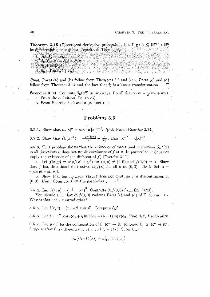
4 0 C h a p t e r 3: T u b D i f f e r e n t i a l

T h eo rem 3.15 (Directional derivative properties). Let f , g : U C Rm —> Rn be.differentiable at x and a a constant. Then at x,

a. dh(af) = adî. . . -b.' 5h (f + g ) = 9hf + 5hg-c. dahf = adhf.d. 0h+kf = dhf + 9kf.

Proof. Parts (a) and (b) follow from Theorems 3.8 and 3.14. Parts (c) and (d) follow from Theorem 3.14 and the fact that f* is a linear transformation. □

E x erc ise 3.34. Compute <?h(x2) in two wavs. Recall that v -w = '( v w + wv).a. From the definition, Eq. (3.23),b. From Exercise 3.29 and a product rule:.

P roblem s 3.5

3.5.1.. Show that c)u |x |“ = 'a x * u |x |“ -2 . Hint: Recall Exercise 3.34.

3.5.2. Show th a t dh(x ~ l ) = + pp-i Hint: x -1 = x |x |- 2 .

3.5.3. This problem shows th a t the existence of directional derivatives 9u/ (x ) in all directions u does not imply continuity of / at x. In particular, it does not imply the existence of the differential /£ (Exercise 3.17).

a. Let / ( x , y) = x 2y / ( x 4 + y2) for (x, y) ^ (0,0) and /(0 ,0 ) = 0. Show that / has directional derivatives <9u/(x ) for all u at (0,0). Hint: Set u

■'■•i + sin#j).b. Show that. lim(Xi3/)_>(o,o) -f(x, y) does not exist, so / is discontinuous at

(0,0). Hint: Compute / on the parabolas y = ax2.

3.5.4. Let f ( x , y ) — (x3 + J /^ )3. Compute <)h/(0,0) from Eq. (3.23).You should find that <?i,/(0,0) violates Parts (<;) and (d) of Theorem 3.15.

Why is this not a contradiction?

3.5.5. Let f (r,0) = (rco s0 ,rs in 0 ) . Compute .

3 .5 .6. Let f = x 2 cos(y)ei + y I n ^ e o + (y + 1) ln(x)e.-}. Find <9hf- Use SymPy.

3.5.7. Let g o f be the composition of f : ]Rm —> Rn followed by g : 1R” -> Mp. Suppose that f is differentiable at; x and g at f(x). Show i itat

((s ° t ) (x )) ~ tsf(x)(ûf lx ))-

S e c t i o n 3 .6 : * I n v e r s e a n d Im p l i c i t F u n c t i o n s 4 1

3.6 *Inverse an d Im plic it F unctions

This optional section discusses two fundamental theorems of vector calculus, the inverse function theorem and the implicit function theorem. Their proofs are difficult, and will not be given. The theorems will be cited only infrequently later in the text. If you choose not to read this section, simply accept th e citations.

T he Inverse Function T heorem

We recall the basic facts about inverses of scalar functions.

Example 1 . y = f ( x ) = x 2, 0 < x < 2, has an inverse,/- 1(y) = y s , 0 < y < 4. See Figure 3.2. The inverse function has a continuous derivative Observe that f'.(x) = 2x ^ 0 for 0 < x < 2. .

Example 2. f ( x ) = x 2, —2 < x < 2, does not have an inverse. For / is not one-to-one: / ( —£') = f ( x ) = x 2. Observe that / ' ( 0 ) = 0 .

T h e o re m 3.16 (Scalar inverse function theorem). Let y = f ( x ) be continuously • differentiable on a < x < b, with f ' ( x ) ^ 0 there. Then f ~ 1(y) exists and is continuously differentiable for f (a ) < y < f(b).

According to the theorem, the condition f ' ( x ) ^ 0 is sufficient for the existence of / -1 . But it is not necessary: f ( x ) = ■%"*, —1 < x < 1 has inverse

/ - 1(y) = even though / ' ( 0 ) = 0 .

E xerc ise 3.35. Show that under the conditions of the theorem, (f ~ 1)'(y) = (/'(a ;))-1 . In less detail: ( / -1 y = ( / ,)-1 * In words: The derivative of the inverse is the inverse of the derivative. Hint: f ~ l {f{x)) = x.

T h e o re m 3.17 (Inverse function theorem). Suppose th a t f : Mn -> En is continuously differentiable in an open set containing a point a. By Theorem 3.6, f£ exists. Suppose that it is invertible.

Then there is an open set A containing a and an open set B containing f(a) such that, f : A —> B has a differentiable inverse f~ ] : B —» A.

The theorem states that if f is continuously differentiable near x = a and, fx has an inverse at x = a., then f has an inverse near x = a. Recall that has an inverse if and only det(f ') J- 0 (LAGA Theorem 8.24b).

1 1Note that, the function . .7:9) = (xf, has inverse f - 1(i/i, 1/2) — (j/jJ , y'i )

everywhere, even though [f(00)] — 0; *he zero matrix, is not invertible.


The theorem becomes more concrete if we write out the components of f:

Vi = f i ( x i , x2, . . . x n), 1 < i < n.

Under the hypotheses of the theorem there is a neighborhood of eacli t/i in which the x 's are functions o f the y ’s:

Xi = 9i{y\ ,y-2, • • • yn), 1 < 1 < n.

E xerc ise 3 .36. Let u — 2xy and v = x 2 —J/2-a. Find all points ’(xo,yo) at-which the inverse function theorem guarantees

that (x ,y ) is a function of (u.v) in some neighborhood of (2.To?/o, x 2 — y2).b. Without solving for (x ,y) in terms of (u,v), find d x /d u , dx /dv , dy/du,

dy/dv. Your answer will be in terms’of x and y. Substituting a given x and y will give the partial derivatives sought; .

The inverse function theorem is only an existence theorem: it guarantees the existence of f _1(y) but does not tell us how to find it. Usually we cannot find the inverse explicitly, so we have to rely on numerical techniques.

The hypotheses of the scalar inverse function theorem guarantee that / is 1 — 1 on the open interval a < x < b. Thus / is invertible on the entire intervala < x < b.

The hypotheses of the vector inverse function theorem do not guarantee that f is 1 — 1 oil the open set U. Thus f need not be invertible on all of U . This is why the theorem only states th a t f -1 exists on a neighborhood of b. We say that f has a local inverse. Exercise 3.28 provides an example: even though f(r g) is invertible for r ^ 0 and all 6, f is not 1 — 1 on the open set of all (r, 6) with r 0. For f (r, ff) = f(r, 9 + 2tr).

E x erc ise 3.37. State Theorem 3.17 for a linear transformation f.

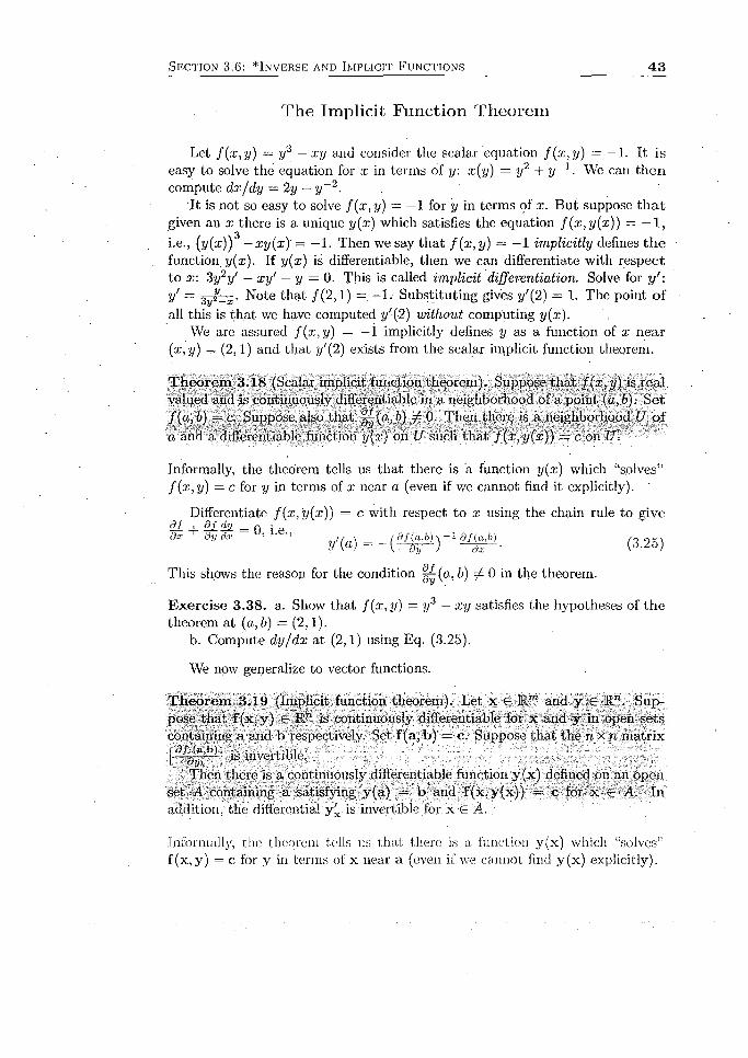
S e c t i o n 3 .6 : ^ I n v e r s e a n d Im p l i c i t F u n c t i o n s 4 3

T he Im plicit Function Theorem

Let f ( x , y ) = y3 — xy and consider the scalar equation f ( x , y ) = —1. It is easy to solve the equation for x in terms of y: x(y) = y 2 + y ~ l . We can then compute dx/'dy = 2y — y~2. '

I t is not so easy to solve f { x ,y ) = —1 for y in terms pf x. But suppose th a t given an x there is a unique y(x) which satisfies the equation f ( x ,y ( x ) ) = —1,

i.e., (y(x))3 — xy{x) = —1. Then we say that f ( x , y ) = —1 implicitly defines th e function,y(x). If y(x) is differentiable, then we can differentiate with respect to x: 3y2y' — xy ' — y = 0. This is called implicit differentiation. Solve for y ' : y' = 3 j^ j.• Note that / ( 2 , 1) = .—1. Substituting gives y'(2) = 1. The point of all this is th a t we have computed y'(-2) without computing y(x).

We are assured f ( x , y ) = —1 implicitly defines y as a function of x near (x ,y) — (2,1) and that y'{2) exists from the scalar implicit function theorem.

T h eo rem .3.18 (Scalar implicit function theorem). Suppose th a t f ( x . y ) is.real valued and is continuously differentiable in a neighborhood of a point (a, b). Set f(a ,b) — c. Suppose also that | ^ ( a,b) ^ 0. Then there is a neighborhood U of

a and a differentiable function y(x) on U such th a t f ( x , y ( x ) ) = c on U.

Informally, the theorem tells us that there is a function y(x) which “solves” f ( x , y) = c for y in terms of x near a (even if we cannot find it explicitly).

Differentiate /( :r, y{x)) = c with respect to x using the chain rule to gived £ , 8 £ d y = 0 ■

9ydx ' = (3.25)

This shows the reason for the condition | {j(a,b) / 0 in the theorem.

E xercise 3.38. a. Show that f ( x , y) = y 3 — x y satisfies the hypotheses of the theorem at (a, b) = (2,1).

b. Compute dy/dx at (2,1) using Eq. (3.25).

We now generalize to vector functions.

T h e o re m 3.19 (Implicit function theorem). Let x € Km and y € R". Suppose th a t f(x , y) 6 Rri is continuously differentiable for x and y in open sets containing a and b respectively. Set f(a, b) = c. Suppose that the n x n matrixrdâjb)-) JjjygftjjljlgL o y k J

Then there is a continuously differentiable function y(x) defined on an open set A containing a satisfying y(a) = b and f(x ,y (x )) = c for x € A. In addition, the differential y* is invertible for x e A.

Informally, the theorem tells us that there is a function y(x) which “solves" f(x ,y ) = c, for y in terms of x near a (even if we cannot find y(x) explicitly).


E xercise 3 .39. Show that Xij/i + £22/12/2 = 2 and x \ y j + xjt/l" = 2 implicitly define (yi, y2) as a function of (xi, X2) in a neighborhood of (xi, x 2) = (1, 1). Hint: Set x = (x i ,x 2), y = (2/1, 2/2) and

/i(x,y) = xiyi + x 2y\y 2 , ' h { x , y ) = x iy \ '+ x ly t -

Define f(x ,y ) = ( / i ( x ,y ) , / 2(x ,y)). Set a = (1,1.), b = (1,1), and note that f(a, b) = 0 .

The implicit function theorem says that if f(x , y) is differentiable near (x, y) = (a. b) and [f^-] is invertible at (a, b), then the implicit relation

f(x ,y ) = c defines a function y(x) near (a ,b ). We made a similar remark following the inverse function Theorem 3.17.

The theorem’s importance lies not just in showing the existence of y(x), but that the derivatives can be computed without computing y(x). Thus we can answer the question: If x changes a little, then approximately how much does y change?

To see how this works, differentiate the n components of f (x, y(x)) = c with respect to x,j using the chain rule aiid write in matrix form:

Since = [§£] [ f f j] (matrix multiplication) and [ ^ j ^ ] is invertible,

we solve for [y^j =

rd / i ( a ,b ) '-1

d f i(a ,b )

dyk L d x -j .

Compare this to the scalar case, Eq. (3.25). Written out, the equation reads

r d y \ (a) 9y i ( a ) - rdfi(a,b) & /i(a ,b )- i - l r d f i (a ,b) d f i ( a , b ) “id x i {)xrli dy \ d y 7l. Ox i Ox-,,,

dy„( a) 0y„(a) a / „ ( a ,b ) d f n (aA)) 3 /„ ( a , b ) d f 7l( a ,b )- 9 x„, J L S y i 0y„. L d x i dx™ J

The matrix sizes are n x m = (n x n) x (» x ra).

E xercise 3.40. Refer to Exercise 3.39. Compute [yf?

The implicit function theorem has many practical applications. One example comes from t he Global Positioning System (GPS): "The. implicit function theorem can be used to answer a key question in the design of the system: approximately how accural,e must time be kept in order to achieve a specified accuracy of location?”-

“ (In.i l N o r r l . D a v id J a b u n , a n d J o h n N o rd , ' I ' lu. C lb lud Po.sl l iordi i . i ] Sijsl.tun, a m i U u , h i i p l i n i l

i m u l u r i i Theorem . SIAA1 U.eview 4 0 ( I 905).

S e c t i o n 3 .6 : În v e r s e a n d Im p l i c i t F u n c t i o n s 4 5

Problem s 3.6

3.6.1. a. For which p,<t>,8 does the inverse function theorem guarantee a local inverse to the function (p , 8 ,0) i-» (x , y, z) of Problem 3.3.3?

b. Determine d p /88. Use Theorem 3.12 and SymPy.

3.6.2. Compute [f£] for the example of Exercise 3.39 in terms of derivatives of / 1 and f 2. P u t your result in the form “m atrix + matrix X matrix”.

3.6.3. a. Let f ( x , y ) = ysin(xy). Show th a t f ( x , y ) = 0 implicitly defines a function y{x) in a neighborhood of ( l , 7r ) .

b. Find y'( 1 ) using’Eq. (3.25).

3.6.4. a. Show that Xiy2'+ X2?/i = 1 and X\Xi = y \y2 implicitly define (j/i, t/2) as a function of (X i ,x 2) in a neighborhood of ( x i1X2, y i , y 2) (1 , 0 ,0 , 1).

b. Compute [y^J, where a = (1,0) and b = (0,1).c.. Using your answer to Part (b), determine d y^ /d x i at a = (1 ,0 ). ■

3 .6.5. Compute [y^J for the functions

x m + x 2y^y2 + X i y m = 4 , x 1y f + x%y% + y3 = 4, x \ + x \ + y\ + y\ + y\ = 8

when a = (1,1) and b = (1,1, 2). Use SymPy.

3.6.6. Suppose that f (u , v, w) is continuously differentiable. Define F(x, y, z ) = f (u (x , y, z ) ,v(x , y, z), w(x, y, z)), where u = x — y, v = y — z, and w — z — x. Show that d F /d x + d F /d y 4- d F /d z = 0 .

3.6.7. Suppose that f ( x , y, z) is continuously differentiable in a neighborhood of (x0, yo, zq) and that none of § | , §~, § | is zero at (x0, yo, ô)-

Show that f ( x , y , z ) = 0 defines functions x = x (y ,z ) , y — y ( x , z ), and z — z(x ,y) in neighborhoods of (yo,Zo), (xq, zq), and (x Q,yo) respectively.

3.6.8. The inverse and implicit function theorems can be proved from each other. The most economical approach is to prove the inverse function theorem first and then prove the implicit' function theorem from it. Show the converse, that the implicit function theorem implies the inverse function theorem. Do not worry about continuity and differentiability conditions. Hint: Let y = f (x) satisfy the hypotheses of the inverse function theorem and consider F(pc, y) =

x-f(y).

Chapter 4

Tangent Spaces

4.1 M anifo lds

There.is a small problem with the sphere parameterization of Eq. (1.5): when. (j) = 0 or 7r (north and south poles), 6, and the parameterization with it, is undefined. It is not unusual that no single function x (u 1,u 2) can parameterize a whole surface. Then we need the concept of a manifold, where more than .one x is used to do the job. This is a fundamental concept in more advanced mathematics.

There is also the question of boundaries. If x : A C K2 —> S C M3 parameterizes a surface do we include the boundary of A in the domain of x? To do so properly we need the concept of manifold with boundary.

Nevertheless, we will call our parameterized objects manifolds as a convenient term, using the name loosely.

We now generalize the notion of a parameterized manifold to higher dimensional objects and higher dimensional spaces. The generalizations are natural.

Equation (1.1) parameterizes curves C in R3, Here is the general parameterization of a curve C in K” . As elsewhere, x is understood to be onto the

manifold‘ x ( « M c i i ' ^ c r . (4.1)

For example, x(t) = ti 4-12j + t3k + i41, 0 < t < 2 parameterizes a curve in R 4, where { i,j,k , 1} is an orthonormal basis.

E xerc ise 4.1. Give the general parameterization of a curve in K4 similar to Eq. (1.2).

Equation (1.4) parameterizes surfaces S in R3. Here is the general parameterization of a surface S in Rn:

x(u, v ) : A C Ikv- —y S c iR". (4.2)

For example, x(u, v) = 3ui-t-(u-v)j —(u2+i/2)k+7ul, 1 < u, v < 4 parameterizes a surface in R4.

4 8 C h a p t e r 4: T a n g e n t S p a c e s

E xercise 4 .2. Give a general parameterization of a surface in R 4 similar to Eq. (1.4). /

We can also parameterize solids B in R3. The identity function i: B —> B. defined by i(x) = x always works. But this is not the only possibility. For.

. example, here is a parameterization of a solid ball of radius r by letting p. vary in the sphere parameterization in Eq. (1.5):

= p siiKpcosOi + psin^>sinf?j + p co s 0 k,

0 < 7r, 0 < 0 < 2tt.

Here is the. general parameterization of a solid B in R”:

x(«, v, w ) : A C R 3 B C R".' (4.3)

Equations:(4.1), (4.2), and (4.3) parameterize 1-, 2-, and 3-dimensional manifolds in R". We can also parameterize manifolds of higher dimension. ■ For example, this is a parameterization of the 3-dimensional boundary of the 4- dimensional ball of radius p in R4:

x(«/\ <j>,9) = p cos tp i + p sin V; sin <j> cos 6 j + p sin ip sin <f> sin 6 k

+ p sin ip cos <61, 0 < tt> 0 < <b < tt, 0 < 6 < 2tt.

E xerc ise 4 .3. Give a general parameterization of a solid in R4 similar to those in Exercises 4.1 and 4.2.

Finally, liere is the general parameterization of an m-dimensional manifold M in R n , m < n:

x( t£ j , //o. . . -, itjn) • C Rm —>■ M C R n . (4.4)

The parameter space A always has the same dimension m as the manifold M , Expanded with respect to a basis this becomes x ( m 1 ; u 2 , . . - , u m) = Xj(ui , u<2 , Urn)&i, where the sum runs from 1 to n.

We will call 1-dimensional manifolds curves, 2-dimensional manifolds surfaces, and 3-dimensional manifolds solids, no matter in which Rn they reside.

Manifolds need not be curved. See the comment at the start of Section 1.2.

R equirem ents for M anifold Param eter Functions

F irs t , th e p a ram ete r functions x m ust have differentials, i.e., be differen

tiable. We need this so we can apply 1-he cl lain rule (Theorem 3.10) and relate

directional derivatives to differentials (Theorem 3.14). This is analogous to requiring th a t scalar functions / have derivatives f (P rob lem 3.3.1). •

Second, the differentials must be one-to-one. Thus tliev have inverses and map linearly independent vectors to linearly independent vectors (LAGA Theorem S.H). This- implies that manifolds have tangent spaces. Wc will see this lor curves and surfaces in the next two sections. See also Problem 4.3.7.

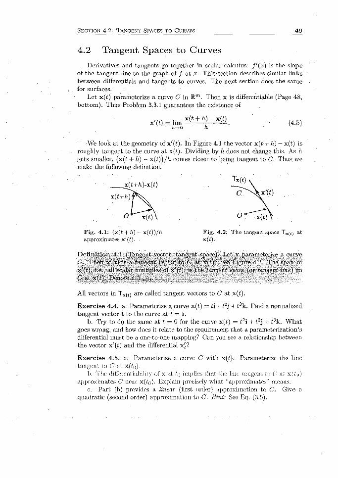
S e c t i o n 4 . 2 : T a n g e n t S p a c e s t o C u r v e s 4 9

4.2 T angen t Spaces to C urves

Derivatives and tangents go together in scalar calculus: f ' ( x ) is the- slopeof the tangent line to the graph of / at x. This section describes similar links between differentials and tangents to curves. The next section does the same for surfaces.

Let x(£) parameterize a curve C in Rm. Then x is differentiable (Page 48,

We look at the geometry of ~x!{t). In Figure 4.1 the vector x(£ + h) — x(i) is roughly tangent to the curve at x(i). Dividing by h does not change this. As h gets smaller, (x(i + h) - x ( t ) ) /h comes closer to being tangent to C. Thus; we make the following definition.

x '(/) . i.e.. all scalar multiples of x '(0 , in 1111' Itmtjrvl i-imn (or innii'iit line) to C ill x(/). Denote il "lxf, j.

All vectors in Tx(t) are called tangent vectors to C a t x(£).

E x e rc ise 4.4. a. Parameterize a curve x(£) = t\ + £2j + t3k. Find a normalized tangent vector t to the curve at t = 1 .

b. Try to do the same at t = 0 for the curve x(i) = t 2i + 12j + t3k. W hat goes wrong, and how does it relate to the requirement that a parameterization’s differential must be a one-to-one mapping? Can you see a relationship between the vector x'(£) and the differential x't?

E x erc ise 4.5. a. Parameterize a curve C with x(i). Parameterize the line tangent to C at; x(/:(-,).

b. The differentiability o fx at to implies that the line tangent to C at x(£o) approximates C near x(to)- Explain precisely what “approximates” means.

c. Part (b) provides a linear (first order) approximation to C. Give a quadratic (second order) approximation to C. Hint: See Eq. (3.5).

bottom). Thus Problem 3,3.1 guarantees the existence of

(4.5)

F ig . 4 .1 : (x(£ + h ) - x ( i ) ) / / i approximates x '(t). .

F ig . 4 .2: The tangent space Tx(t) at x(t).

50 C h a p t e r 4 : T a n g e n t S p a c e s

B asic Facts abou t x'(£)

T h eo rem 4.2. Let x(£) = (x.i(t),x2( t ) , . . . , x m (t)) e Rm. Then x '( t) exists if and only if all x'^t) exist. If they do exist, then x '(t) = x 2(t) , .. . ,x'm (t)).

Proof. For ease of notation, let x(i) = (x(t),y(t)) G M2. Then

*-(,) = Bm *<« + - *<*>fc-»o h

- iirn (x(f + + h)) - (x (t),y(t)) ■h-iO h

— limh—

X(t + h) - x(t) y(t + h) - y( t) \

h ’ /i /

-j—------ , u n i --------------------it h— h, J

= (x '( t ) ,y ( t ) ) .

The limit on the left side of Step (4) exists if and only.if the limits on the right side do (Theorem 2.till). The other equalities are always valid. □

Theorem 4.3 (Product rule). Let Xi(/,) and (t) parameterize curves and suppose th a t x^(t) and x 2(t) exist. Then (x ix 2) (t) exists and

( y n x 2) \ t ) = x ’l ( t ) x 2( t ) + x 1( t ) x 2(t).

Since the geometric product is not commutative, the order of the factors is important.

We have defined the derivative x'{£), where x ( t ) G R” (Definition 4.5). But we have not defined the derivative (x ix 2 )'(t), where ( x i x 2)(t) € Gn . However, since limits make sense in Gn (Definition 2.5), we can define (x jx 2)'(i) as we did x'(t) . In a similar way, for example, Definition 3.5 of a differential can be extended to functions taking values in G".

There are analogous rules to Theorem 4.3 for the inner and outer products:

(x i • x2 )'{f) = x \ ( t ) - x 2 (t) + X j ( t ) - x 2 (i), (4.6)

(x, A x 2)'(i) = x', (t) A x-2 (/) + x, (/) A x 2(/)

E xerc ise 4.6. Prove Theorem 4.8. Hint: Look at the proof of the product rule for derivatives in scalar calculus.

E xerc ise 4.7. Let x(t) parameterize a curve which does not go through the origin. Let x(*o) be a point on the curve closest to the origin. Show that x(f0)and x'(l.u) are orthogonal.

S e c t i o n 4 . 2 : T a n g e n t S p a c e s t o C u r v e s 5 1

T h e o re m 4.4. Let x(t) parameterize a curve in R"1.

a. Show th a t |x(/.) ^ .x(/.). = x(t) ■ x '(t) .

b. Show th a t if |x(£)| is constant, then x'(t) ± x(t).

According to Part (b), if x(t) is confined to a sphere, then x '(t) is orthogonal to x(f). In other words, the tangent vector is tangent to the sphere. ©

E xerc ise 4 .8 . Prove Theorem 4.4. Hint: For Part (a), use |x |2- = x - x .

Angular V elocity

• Rotate a vector x G M3 in a time dependent manner: x(t) = R (t)xoR ~l (t), where R(t) = e_ 1 sW/ 2 (LAGA Section 7.2). Both i and B are functions of t. Then ~

x' = R.xo{Rr1y + R ,x 0R - 1 (4.7)

= - ( R x o R r ^ i R ' R - 1) + (R . 'R r l ) (R x 0R r l ) = § (xfi - Ox) = x ■ U.

Step (1) is Theorem 4.3. The first term on the right side of Step (2 ) is obtained by differentiating R R r 1 = 1. Step (3) defines

' f i = - 2 R.'R.r1. . (4.8)

Step (4) uses the fact that f i is a bivector (Problem 4.2.4 and LAGA Eq. (7.13)).

E x erc ise 4 .9. Set u> = Cl*, the dual of f i, a vector. Show that

x = U) x x.

We seek a geometric interpretation of uj. Consider first a counterclockwise rotation about a fixed axis. See Figure 4.3. The circle is the path of the endpoint of x . The vector x ' is in the plane of the circle and tangent to it. Equation (4.9) shows that u> is orthogonal to x ' everywhere on the circle. Thus it is orthogonal to the circle, as shown in the figure. So it is the axis of rotation. And f i is the plane of rotation.

Differentiate the defining equation of radian measure on the circle: § = r § . Then

(4.9)

Fig. 4.3: Rota-

dx. ds dB tion about a fixed—

dt dtaxis = fi*.

Also, Eq. 4.9 shows that

Ix'l = Iw x x| |w| |x| sinc/i

Compare the two expressions for jx'| to see th a t . |w| = the angular velocity. Call u> the angular velocity vector.

If the rotation is not about: a fixed axis, then u> is still called the (instantaneous) angular velocity vector and fi the (instantaneous) angular velocity bivector.

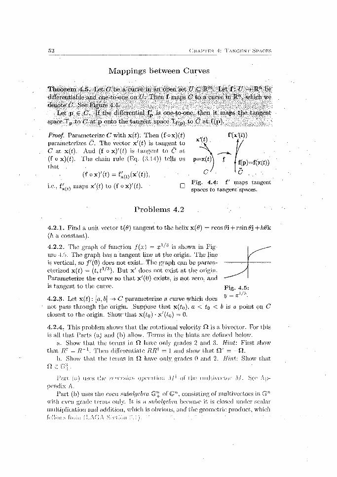
52 C h a p t e r 4: T a n g e n t S p a c e s

M appings b etw een Curves

T h eo rem 4.5. Let C be a curve in an open set U. C Km. Let f : J/ -> Rn be differentiable and one-to-one on U. Then f maps C to a curve in JKn, which we denote C. See Figure 4.4. .

Let p £ C. If the differential fp is one-to-one, then it maps the tangent space Tp to C at p onto the tangent space Tf(p) to C a t f(p).

Proof. Parameterize C with x(t,): Then (f ox)(£) f'(x'{i))parameterizes C. The vector x'(t) is tangent to C at x(£). And (f o x)'(f) is tangent to C at (f o x)(t). The chain rule (Eq. (8.14)) tells us that

(f ox ) '( t) = f£w (x'(t)),

f(p)=f(x(i))

C . .

, ,, . , w . _ Fig. 4.4: f maps tangenti.e., maps x (i) to (f ° x) (£). □ • . , ,‘ v ' v ' v ' spaces to tangent spaces.

P roblem s 4.2

4 .2 .1 . Find a unit vector t(Q) tangent to the helix x{6) = 7-cos#i + 7'sin +h6k (.h a constant).

4.2.2. The graph of function f ( x ) — x l-/4 is shown in Figure 4,5. The graph has a tangent line at the origin. The line is vertical, so / '(0 ) does not exist. The graph can be parameterized x(/;) = (t, t l lA). But x ' does not exist at the origin.Parameterize the curve so th a t x'(Q) exists, is not zero, and is tangent to the curve. p jg_ 4 5 .

V = x l '/34 . 2 .3 . Let x ( t ) : [o,6j -> C parameterize a curve which doesnot pass through the origin. Suppose th a t x(to). a < to < b is a point on C closest to the origin. Show th a t x(fo) • x ' f a ) — 0.

4 . 2 .4 . This problem shows th a t the rotational velocity f t is a bivector. For this is all that Parts (a) and (b) allow. Terms in the hints are defined below.

a. Show th a t the terms in f t have only grades 2 and 3. Hint: First show that /?* = R ~ l. Then differentiate R,R* = 1 and show that f t *1 = —ft.

b. Show th a t the terms in f t have only grades 0 and 2. Hint: Show that f t e G l .

Part, (a) uses the reversion operation AP of tin; lnullivecior M. See Appendix A.

Part (b) uses the even subalgebra G"_ of G", consisting of multivectors in Gn with even grade terms only. It is a subalgebra because it is closed under scalar multiplication and addition, which is obvious, and the geometric product, whichioliows [roiii i LAGA ' ■f■ ’ ! i1111 .....; j.

S e c t i o n 4 .3 : T a n g e n t S p a c e s t o S u r f a c e s 5 3

4.3 T angen t Spaces to Surfaces

Let x(u, v ) : A C R2 —> S C ]Rm parameterize a surface. Then x is differentiable (Page 48, bottom). Figure 4.6 shows a vector w in the uu-plane with tail at q. Consider the directional derivative (Eq. (3.23))

x (q + hw ) - x(q)

x q (w )

5wx(q) = lim h —f 0 h

(4.10)

Recall that 9wx(q) = x'q(w) (Eq. (3.24)). Fig’ 4’6: The tangent space Tp'If h is small, then x ( q + hw) — x(q) is the difference between nearby points

on S and so is nearly tangent to S at p . Thus we make the following definition.

D efinition: 4.6 (Tangent vector, tangent space). Let x : A C R - —> 5 G: parameterize a surface. Let q G A and set p = x(q). Then the vector x^(w) is a tangent vector to S at p . The set of all tangent vectors at p is the tangent space (or tangent plane) to S at p. Denote it Tp. See Figure 4.6.

Recall th a t the differential must be x^ is one-to-one and map linearly independent vectors to linearly independent vectors (Page 48, bottom). Thus the tangent space to the 2-dimensional surface is 2-dimensional © .

A basis for Tp. In Figure 4.7, i and j form an orthonormal basis in the uu-plane. Since they are linearly independent, so are x q(i) and X q ( j ) ,

which therefore form a (not necessarily orthogonal) basis for T p. Now

x q(i) = dix(q) = d„x(q) = x u(q).

Step (1) is Eq. (3.24). Step (3) introduces the new notation x u = <9„x. A similar calculation shows that x^(j) = x„(q). Thus we learn the important fact that {xu,x„} is a basis for T p.

The bivector x u Ax^ is a pseudoscalar of the geometric algebra of the tangent space Tp.

In R3 the dual of x„ Ax„ is normal to S, i.e., normal to its tangent space:

n = (xu A x v)* = x u x x„.

There is no unique direction normal to surfaces in Rm, m > 3.

(4.11)

E xercise 4.10. a. Consider the parameterization of the hyperbolic paraboloid from Problem 1.2.3: x(u ,v) — (u+v)i + (u —v)j+4uvk. Find a unit pseudoscalar of the tangent space to the surface at x ( i , 1).

b. Find the equation of the plane tangent l:o the surface at x ( l , 1).

5 4 C h a p t e r 4: T a n g e n t S p a c e s

E xercise 4.11. a. Let x(u, v) parameterize a surface S. Parameterize the tangent space to S at x(uo, «o).

b. Since x is differentiable at (uo,Uo), the plane tangent to S at x(uo,vo) approximates S' near x(ii0, t'o). Explain jprecisely what “approximates” means.

c. Part (b) provides a linear (first order) approximation to S. Give a quadratic (second order) approximation to S. Hint: See Eq. (3.5).

x i ■ .Vi + f ( x , J/)k isE xerc ise 4 .12. Let z = f ( x , y ) represent a surface S.

a. Give conditions th a t tiie parameterization x(x, y) differentiable at (Xo,yo)■

b. Find a pseudoscalar of the tangent space above the point (xo,?/o)-c. Show th a t a normal vector to the surface above the point (x<>, yo) is

d f(xo ,yo ) . d f ( x 0.y Q).'n = ------ ^ ------- i ---- —4:----- 4-k.

dx dy

d. Show that the equation of the plane tangent to the surface at the point (:»•:•.. //.». f ( r,.. //.,)) is

'.f(x0,y0) +d f ( x 0,y 0)

dx ■(x - x0)

d f ( x 0,y 0)

dy ( y - y o ) -

Since the plane tangent to the surface approximates the surface, this provides a linear approximation to f ( x , y ) near (xo,yo).

Let C s be a curve on S through p. See Figure 4.8. Then C s is the image by x of .a curve C \ in A. If w is tan gent to C a at q, then x q(w) is tangent to Cs at p (Theorem 4.5). By Definition 4.6 it is also in T p. We have learned an interesting fact: All tangent vectors to curves in S through p, no m atter how they behave at p, lie in a single plane, T p.

Xq(w)

F ig . 4 .8 : The vector x ^ (w ) is tangent to the curve Gs at p.

S e c t i o n 4 .3 : T a n g e n t S p a c e s t o S u r f a c e s 5 5

M appings betw een Surfaces

T h e o re m 4.7. Lot S be a surface in an open set U C ]Rm. Let f be a one-to-one differentiable map on U to Rn. Then f maps S to a surface S in Kn. Let p € S .

If the differential is one-to-one, then it maps the tangent space Tp to S onto the tangent space Tf(pi to S. See Figure 4.9.

Theorem 11.11 will improve this theorem, by requiring only th a t f be defined on S instead of an open set containing S.

Proof. Parameterize S with x ( m , ?;).Then (fox)(u, v) parameterizes S. The vector Xq(w) is tangent to S' at p = x(q). And (fox)q(w) is tangent to S at

■ (f o x)(q). The chain rule (Eq. (3.14)) tells us that

(f ox)q(w ) = fp(x^(w )),

i.e., fp maps x^(w ) to (f ox)q(w). □

P ig . 4 .9 : f' maps tangent spaces to S to tangent spaces to S.

fp(x„ A x„) = fp(xu) A fp(x,,),

i.e., fp maps the pseudoscalar x u Ax v of Tp to the pseudoscalar fp(xu) A fp (x ^ ). of T f(p).

The notion of tangent spaces to curves and surfaces extends to tangent spaces to higher dimensional manifolds. At each point p in an m-dimensional manifold, there is an m-dimensional tangent space Tp. See Problem 4.3.7.

Theorems 4.5 and 4.7 extend to higher dimensions. Skipping the technical niceties, we have:

Let f be a one-to-one differentiable map between manifolds of equal dimension.

Then fp maps Tp to Tf(p).

We can explicitly express the mapping of tangent spaces in Theorem 4.7 as the outerinorphism extension of

5 6 ClIAPTKR 1: TANGENT SPACIiS

P roblem s 4.3

4.3.1. a. Parameterize a sphere with Eq. (1.5). The plane tangent to the sphere at the equator (<j> = 90°) is (—siriê1+ c o s^ e 2 )A e3 . Explain this geometrically.

b. Find the tangent space x u A x t, at an arbitrary point. Use SymPy.c. Find a normal vector n to the sphere using Eq. (4.11). Use SymPy.d. Your answer to Part (c) should be a scalar multiple of the vector param

eterizing the sphere. Explain this geometrically.

4.3.2. Find an equation of the plane tangent to the surface x 2 + y 2 — z 2 = 1 at the point (x0,y0, z 0). .

4.3.3. Show that;, all planes' tangent to z = x f ( y / x ) , x ^ 0 pass through the origin. '

I4.3.4. a. Approximate {(3.01)2 + (3.98)2) - . Do not use technology. Ans. 4,99.

b. Explain what the plane tangent to f ( x , y ) = (x 2 + y2) i at (3,4) has todo with the answer to Part (a).

4.3.5. W hat are the tangent spaces to a solid in K3? Hint : First determine the dimension of the tangent spaces.

4.3.6. In Theorem 4.7, the differential fp maps the tangent space Tp to S to the tangent space Tf(p) to S. Let i be the unit pseudoscalar of Tp and i the u n it. pseudoscalar of Tf(P). Let J be the Jacobian determinant, of f at p: J = det[fp]. Show that J = fp(i)/i. Hint: The solution uses two definitions concerning determinants from LAGA (only).

4 .3 .7 (Tangent spaces to m-dimensional manifolds). Parameterize an Tridimensional manifold M in K" by x(u), where u = (u i ,u 2, .. - ,u m) G A C Rrn, As u varies over A, x (u) varies over M.

a. Define the tangent space to M a t x(q) = p.b. Define a pseudoscalar in the tangent space at p.

Chapter 5

The Gradient

5.1 F ields

D efin ition 5.1 (Field). A field is a special.kind of function: For us it is defined on a manifold M (a curve, surface, solid, . . . ) and takes values in some GTl. If the field is scalar, vector, bivector,... valued, then it is a scalar, vector, bivector, ..., field.. ■’

For example, the temperature t{x) over some region M of a country is a scalar field. The wind velocity w(x) over the region is a vector field.

Here is how to think about a vector field f(x) on M.Refer to Figure 5.1. The points x 6 M are the heads of vectors whose tail is a t a common origin (not shown). These vectors “label” the points of M (x t and X2 in the figure).Then for each x place the tail of f(x) at the head of x.

F ig . 5 . 1: A vector field f on M .

E xercise 5.1. Discuss the direction and norm of the field vectors f(x) = x in Figure 5.2.

\ t f i f / /V V v. \ * 1 f f / S X^ X X \ \ t t f / A S / s y ' -

/ / S ' 'j / / ' - I i * ‘} i ‘ 1 * * ' ‘\ ' v \ \ ^ x

\ \ - ' ' \ X ^

^ v. v \ x \ \

- v X V. \. N X \ \. ( \ \ ^. t f t . - I I I , , f t i ^ s / / /~ ^ s / /

. ^ ^ / / /

F ig . 5.2: f (x ) = x. F ig . 5.3: g (x ) is f (x ) rotated 90°.

5 8 C h a p t e r 5: T h e G r a d i e n t

5.2 T h e G ra d ie n t

D efin ition 5.2 (V F ). L e t F b e a d i f f e r e i i t i a b l e m u l t i v e c t o r f i e l d d e f i n e d o n a i l

o p e n s e t C / i n E n . L e t . { e , } b e a n o r t h o n o r m a l b a s i s f o r R ” . T h e n t h e gradient

o f F i s a n o t h e r m u l t i v e c t o r f i e l d o n U d e f i n e d b y

V F ( x ) = e j £ ? j F ( x ) = e i < ? i F ( x ) + e 2 3 2 F ( x ) + • • • + e ndnF(x). ( 5 . 1 )

( P r o n o u n c e V “ g r a d ” o r “ d e l ” . )

The product in e l diF(x.) is the geometric product.

E x e r c i s e 5 . 2 . Compute by hand; V(1 + x j / 2 e i ' + s m y e 2 + s in x c o s jy e ^ ) .

D e f i n i t . i p n 5 . 3 ( V ) , I t i s useful to think of V a s . a n independent entity:

V = e i d i '= e i d i + e 2&2 - f • • • + c n d n

- - a l s o c a l l e d t h e gradient o r gradient operator - w h i c h h a s a n e x i s t e n c e i n d e

pendent of any multivector ou which it may operate.

The gradient V = e ^ is not a vector. But it behaves algebraically as a vector if the di are viewed as .scalar coefficients. That is why it is denoted in bold. Scalars commute. .The' “scalars” di commute when applied to an F with continuous mixed partial derivatives: did jF — d jd jF (Theorem 3.3).

The next exercise provides examples of V behaving a s a vector. Part (a) is “(vector)(scalar) = vector” . P art (b) is “vector • vector = scalar” . ConsideringV a s a vector is an aid to computation. Problem 5.2.7 provides an example.

E x e r c i s e 5 . 3 . a. Show th a t V x , - = c , .

b. Show th a t e z - V = di.

E x e r c i s e 5 . 4 . Suppose th a t F is a / c - v e c t o r valued field.a. W hat is (are) the grade(s) of a - ( V F ) ?

b. W hat is (are) the grade(s) of ( a • V )F ?

T h e o re m 5.4. The gradient is well defined, i.e., independent of the orthonormal basis in which it is expressed.

T o understand t h e meaning o f the t h e o r e m , l e t x = .T,;ef and x = y.jij be the expansion of x with respect to two o r t l i o n o r m a l bases. Let F ( x ) be a differentiable field on R” . The theorem states that

0F(x) OFCx)•Of—:--- - = t ; —----- •

dx, J dyj

We will p rove the m ore general T heo rem 5.14 below.

The gradient is one of very few combinations of derivatives and bases which is independent of the orthonormal basis in which it is expressed. Problem 5.2.1 exhibits a. combination which gives different result vectors with different bases; the result does not depend just on the field to which the combination is applied. No such combination can be of genera,1 interest.

S e c t i o n 5 .2 : T he G r a d i e n t 5 9

E xercise 5.5. Show that V x = n in Rn. In general, (vector)(vector) = scalar •f bivector. Here the bivector part is zero.

E xercise 5 . 6 . Let / be a differentiable scalar function.a. Show that 9j / ( | x | ) = ^ / ' ( | x | ) . Hint: Use the chain rule for scalar

functions and | x | = (xf + . . . x 2 ) 5 . .

. b. Show th a t V /( |x |) = .- | |f / / (|x|).

c. Show th a t V | x | fc = f c | x | f c _ 2 x . Since x 2 = | x | 2 , this gives V x 2 = 2 x .

d. Determine V In |x|.

T h e o r e m 5 . 5 ( V p r o p e r t i e s ) . T , n l . a I n : a s c a l a r r o n s i . ' i n t a n d F a n d G b o

d i f f e r e n t i a b l e i m i l i i w r l u r f i e l d s d e f i n e d o n a r t o p e n s i ' l . U R " . T h e n

a. V ( a i ’) aS/F.b . V ( F + G) = V F + V _ G .

c. V (F G ) = V F G + V F G . (The proof will explain the dot notation.) .

Proof These.follow from corresponding facts in Theorem 3.2.a. V (a F ) = eidi(aP) — aeidiF = a V F .b. V ( F + G) = e A (F + G) = e ^ F + e & G = V F + V G .c. This is the product rule. Start with the product rule for partial deriva

tives: di(FG) = FdiG + [diF)G. Multiply by and sum:

&idi{FG) = eiFdiG + (eidiF)G, i . e . - , V ( F G ) = e ^ G + (VF)G .

We cannot rewrite eiFdiG as FeidiG — F V G because e t and the multivector field F do not in general commute. Thus we write eiFdiG as V F G . The notation tells us to differentiate G but keep the e t a t the location of V . Similarly, we write (V F )G = V F G . □

E x e r c i s e 5 . 7 ; Let f be a vector field. Write f V in terms of components and compare to V f .

E x e r c i s e 5 . 8 . Show that, if a is a scalar field and F is a multivector field, then V (a F ) = a V F + (Va)F .

T h e o r e m 5 . 6 . S u p p o s e t h a t f i s d i f f e r e n t i a b l e a t x . T h e n

d h f ( x ) = ( h • V ) f ( x ) . ( 5 . 2 )

In words: The directional derivative in the direction h is the component ofV in the direction h.

Proof. Set h = /i,e;. .Use Theorem 3.15c, d in Step (2):

d\\ f (x) = dkt(lj f(x) = hide, f(x) - lijd., f(x) = ( h • V ) f ( x ) . □

C o r o l l a r y 5 . 7 (££*). The adjoint of f ' is f ' * ( b ) ;= V ( f ( x ) - b ) (L \G \ Lq ( 8 . 7 ) ) .

Problem 5.2.10 asks you to prove the corollary.


D ivergence and Curl

Use the extended fundamental identity a F = a ■ F + a A F for a vector a and multivector F to separate the gradient V F into two parts: • •

V F = (eidi)F = V • F + V A F, where (5.3)

V - F = (eidi) ■ F = e £ - djF, (5.4)

V A F = ( e ^ ) A F = e ; A <9iF. (5.5)

Call V • F the divergence of F .and V A F the cw / of F . Thus

gradient = divergence + curl..

The divergence is grade lowering: vector - r-vector = ( r—l)-.vector. Similarly, the curl is grade raising.

Vector calculus also defines the divergence V * f of a vector field. In R3 it defines the curl of a vector field as V x f, which is (V A f)*. However, vector calculus cannot unify its divergence and curl into an analog of our gradient V f.

E xerc ise 5.9. a. Show th a t V • x = n and V A x = 0 in R".b. Show th a t V A |x |fc = k |x |fe-2x. Hint: See Exercise 5.5.

Theorem 5.9 below shows that several different combinations of the gradient, divergence, and curl arc zero. They are all essentially statements of the equality of mixed second order partial derivatives (Theorem 3.3), as expressed in this lemma.

L em m a 5.8. Let F be a multivector field on an opcri set U C R” with continuous mixed partial derivatives. Then

a. (e* A Bj) d ijF = 0.,bi- • («* A e /) -A.dtjF .= 0;

Proof. The proofs of the two parts are similar. We prove Part (a).If i = j , then e* A e^ = 0 in the double sum e* A e.j d ^F . If i ^ j , pair the

i j term with the j i term in the double sum (i and j are fixed, not summed):

(ef A ej) dijF 4- (e3- A e ^ c ^ F = (e* A e^) d ^ F - (ei A e ^ d i j F = 0. □

T h e o re m -5.9.. -.Let / be a scalar field and F a multivector field defined in an .open set U C R7!, and having continuous mixed partial derivatives there. Then

a. V A (V A F) -- 0. (The curl of a curl is zero.)b. V A (V /) = 0. (The curl of the gradient of a scalar field is zero.)c. V • (V • F ) -• (!. (The divergence of a divergence is zero.)d. (V A V )F • 0.

Proof, a. V A (V A F ) = (eidl )A (e jd jA F ) = (e.;Ae7)A9.jjF = 0 by Lemma 5.8b.b. For a scalar field / . V / —' V A / , so this follows from Part (a).Exercise 5.Hi asks you to prove Parts (c) and (d). □

S e c t i o n 5 .2 : T h e G r a d i e n t 6 1

E xerc ise 5 .1 0 . Prove Theorem 5.9, Parts (c) and (d).

E xerc ise 5 .1 1 . Show that Theorem 5.9b does not extend to vector valued fields. Hint: Try V A (V x 3) in ]R2.

Vector calculus cannot express Theorem 5.9 because it does not have the outer product. But in R3 it has the cross product. • . ■ • .

T liro rp in ft.10. L e i f be u scalar f i e l d a n d f a v e c t o r f i e l d d e f i n e d i n I ’ i_ P '5, a n d h a v i n g c o n ! i n u o u s m i x e d p a r t i a l d e r i v a t i v e s t h e r e . T h e n

a . V ■ (V x f) ( J . ( T h e d i v e r g e n c e o f t h e c u r l o f a v e c t o r f i e l d i s z e r o . )

i i . V x (V f ) — 0 . ( 1 I k -, u i i i o f t h e ^ r . u l i e n i o f a s c i ' l a r i i e l d i s z e r o . )

Careful: Problem 5.2.7 shows that in general., V • (V A f ) / 0 to Part (a).

in contrast

Proof, a. Starting with Theorem 5.9a,

V A (V A f) = 0 => . (V A (V A f ) )* = 0 => V • (V x f) = 0.

b. Starting with Theorem 5.9b,

V A ( V / ) = 0 => ( V A ( V / ) ) * = 0 =>’ V x ( V / ) = 0. □

Problem 5/2.6 asks you to provide a proof of this vector calculus theorem using only vector calculus.


P roblem s 5.2

5.2.1. Theorem 5.4 shows that e.\dx +e%dy is well defined in R2. This problem shows th a t e \ dx — c^dy is not. Start with a scalar function defined on a plane. Suppose th a t when the function is expressed in terms of coordinates (x ,y), it is represented by f { x ,y ) — x. Then c\Oxf ~ e 2dyf = e i. Let {e j, e'2} = {e2, —ei} be a second basis, a t angle 90° from the first.

a. Represent the function as g(x', y') in the primed system.b. Show that e[dX'g — e'2dy’g ^ e.idxf — e 2dyf .

5.2.2. a. Prove that V (xa) = n a in M". Notational conventions tell us that a is a constant vector here.

b. Prove: V (x • a) = a.Subtracting Part (b) from Part (a), gives V (x A a ) = (n — l)a ,

5.2.3. Suppose that a is a scalar field and F is a multivector field of grade k. Show that

V - (aF) = a V • F + ( V a ) • F a n d V A (aF) = a V A F + ( V a ) A F. .

Hint: See Exercise 5.8.

5.2.4. Show th a t V (x |x |fc) = (n + /c ) |x |fc in Mn. Hint: Recall Exercise 5.6a. Important special case k = —n: V (x / |x |rl) = 0.

5.2.5. Let / be a scalar function. Show that V • (/( |x jx )) = n / ( |x |) f ,/'( |x |) |x |.

5.2.6. Theorem 5.10 was proved using the curl of geometric calculus. Prove the theorem using the cross product of vector calculus.

5.2.7. Let f be a vector field defined in U C R3. Show that V • (V A f) = —V x (V x f). Consider V as a vector, as described on Page 58.

5.2.8. Define the bivector field B = (x 2 -1- y2 + z2)_3//2(:rjk + yki + zij). Show that V A B = 0 . Hint: For ease of calculation, write B = / F, with / = (x2 + y 2 -)- z2)-3/ 2 and F = ,-rjk + yki + zij. Compute V A / and V A F separately, simplify, and then use the curl analog of Exercise 5.8.

5.2.9. Let / be a scalar valued function of x 6 M", which is in turn a function of a scalar t: / (x ( i)) . Show that J j/(x (£ )) = V /(x ) - x'(/;).

5 .2.10. Prove Corollary 5.7. Show that the ad joint of f ' is given by f'*(k) = V (f • k). Hint-. Coinbim: Eqs. (:(. i-i) and ( -r>.2) U> give f^(li) ;■= (li - V )f.

S e c t i o n 5 .2 : T h e G r a d i e n t 6 3

E lec tro m ag n e tism . Electromagnetism is the study of electric charges and the electric and magnetic fields they generate. We compare here the vector calculus and geometric calculus formulations of electromagnetism. For simplicity we restrict ourselves to regions of space away from the charges.

In vector calculus the electric and magnetic fields are represented by vector fields varying in space and time: e = e(x .,y ,z , t) and b = b(z, y, z , t ) , respectively. The fields satisfy Maxwell’s equations, four equations involving the divergence and curl of e and b as functions of ( x ,y ,z ) . These equations are among the most precious we possess, governing the behavior of light, radio waves, motors, the electric grid, etc. At points where there are no electric charges they are1

V - e = 0, V x b = dte, V x e = — 9tb, V - b = 0. (5.6)

F ig . 5.4: A bivector B better represents a magnetic field than does a vector b.

Perhaps the greatest triumph of vector calculus is its formulation of electromagnetism in what are today called Maxwell’s equations. Nevertheless, physical arguments show that the bivector field B = —b* (so b ■ B ') of geometric calculus better represents a magnetic field than b. Figure 5.4 illustrates one example.

Look first at the right side of the figure. The loop is a circular wire carrying an electric current. The current’s direction is indicated by the arrowhead on the loop. The current generates a magnetic field which varies from point to point.

The right side shows a representative vector b orthogonal to the loop and bivector B parallel to the loop. The orientation of b is given by the right hand rule: wrap the fingers of your right and around the loop in the direction of the current and your thumb will point in the direction of b. The orientation of B is given directly: it is that of the current. The area of the parallelogram is equal to the lengtli of the vector.

Now reflect the entire setup in the plane indicated by the dashed line. The orientation of the reflected B is that of the reflected current, which is physically correct. The orientation of the reflected b (shown as “cf” , a reflected “b ”) is not given by the right hand rule. The correct magnetic field vector on the left side is b = — d. Moral: to reflect a magnetic field vector, first reflect it as a vector, and then (don’t forget!) negate it.

Since magnetic field vectors do not behave like vectors under reflections, they are not really vectors. The correct term is pseudovector, or axial vector. The vector/pseudovector distinction is not encoded in the vector space formalism; one'must remember to which type an oriented lengtli belongs. Geometric algebra recasts the distinction as vector/bivector, which is encoded in the formalism.

‘W e use u n i t s o f t im e a n d d is ta n c e so t h e speed o f l ight is 1. For exam p le , t im e m igh t b e m easu red in seconds a n d d is tanc e in l ightseconds, th e d i s ta n c e light trave ls in one second.


5.2.11. a. Reformulate Maxwell’s Equations (5.6) in geometric calculus as

V • e = 0 , V • B = —d t e , V A e = - d tB , V A B = 0 . (5.7)

b. Set e = e ie i +coe2 + e 3e 3 and B = £ 2 3 6 2 6 3 + B n ^ ^ i + B i2e ie 2, Write both V • B = —dtc and V A B = 0 as four scalar equations.using these components. This should help you appreciate coordinate free multivector notation!

We have seen that geometric calculus unites the divergence and curl of vector calculus into the gradient V . In electromagnetic theory it also unites the e and B fields into the electromagnetic field F = e + B. The e and b fields of-vector calculus cannot be united into a single field.

5.2.12. Show th a t the four vector calculus Maxwell’s equations above become one geometric calculus. Maxwell equation, (dt + V )F = 0. Hint: Look at the scalar, vector, bivector, and trivector parts of this equation.

A similar simplification occurs when charges are included.

The single geometric calculus Maxwell equation for a single field F has significant advantages over the four vector calculus equations in two fields, Eqs. (5.6).

We give an example. Define the Laplacian

V 2 = V V = V - V

cf~ cf^. , = (Gidx + e 20y + e 3dz) - (exdx f e 2dy + e3dz) = — + — +

Now start with Maxwell’s equation (dt + V )F = 0 and form

(dt - V )(3 t + V )F = {da - V 2) F = 0.

(The equality of mixed partial derivatives tells us that 9t V F = Vc^F.) The equation (dtt — V 2) F = 0 is called the wave equation because it describes a moving wave. The electromagnetic field F moves as a wave - an electromagnetic wave!

Here is a vector calculus derivation of the wave equation (9W — V 2)b = 0 :

- d ttb = dt ( - d , b) = d,.(V x e) = V x dte = V x (V x b)

.4 V - (V - b) - V 2 b = - V 2 b .

The step's use the equality of mixed partial derivatives and Maxwell’s equations (5.6), except Step (5), which is a vector calculus identify. Another, similar, calculation is required for (dn — V 2)e — 0.

The most natural setting for electromagnetism is the spacetime geometric algebra, a geometric algebra of a slightly different kind inspired by relativitytheory. An electromagnetic field is represented by a bivector field F . At points where (.here are no charges Maxwell’s equations become V F = 0, where V is the gradient operator of spacetime.

S e c t i o n 5 .3 : S c a l a r a n d V e c t o r F i e l d s 6 5

5.3 Scalar an d V ector F ie lds

The gradient V can be applied' to any inultivector field. Scalar and vector fields are the most important. We trea t them in turn.

Scalar F ields

The gradient of a scalar field is

V / = (e id i) f = etd if ,

“(vector)(scalar) = vector” . Expanded in R3 this is

V f = d}f e i + d2f e 2 + d 3f e 3. (5.8.)

We will prove two important facts about gradients of scalar fields, Theo- rems'5.11 arid 5.13. • , ' '

T h eo rem 5.1 ] . L<-|. / be scalar valued and differentiable a t x, with V /(x ) ^ 0. l.i'i I) be 1 he angle b<’iwren V /(x ) and a unit vector u. Then the directional- di'rivnfive i)uf ( x ) is given by

da/ (x ) = |V/(x)]cos6>. (5.9)

See Figure 5.5.

Proof. 8a / (x ) = (u - V ) /(x ) = u - (V /(x ) ) = |V /(x ) |co s0 .Step (1) is Theorem 5.6. Step (2) is valid for scalar fields.(But see Problem 5.3.5.) Step (3) is the definition of the inner product when |u] = 1 (LAGA Eq. (4.1)). □

Fix x and let u vary. The theorem shows that the largest value of 5 q /(x ) is |V /(x ) | when 0 = 0 , i.e., when u is in the direction of V /(x ). As u moves away from this direction, the Fig. 5.5: directional derivative decreases with cos 0 , reaching zero when ô /(x ) =53 is orthogonal to V /(x ). Continuing to move away from I Vf(x)| cosf?. the direction of V /(x ), the directional derivative goes negative, reaching its minimum value — |V /(x ) | when u points in the opposite direction from V /(x ). W hat a simple geometric picture!

E xerc ise 5.12. Suppose that the temperature in a region of the plane around (0,0) is t(x ,y ) = 100 - (;rr2 + 2y2).

a. If Pablo is a t the poin t ( 2 , 1), in which direction should he move to warm

up most rapidly?b. W hat is the most rapid rate of increase?


L em m a 5.12. Let / be a continuously differentiable scalar valued function on an open set U C R". Let xo € U and suppose that V / ( x q ) ^ 0. If /(x o ) = c then / ( x ) = c implicitly defines an (n-T)-dirncnsional manifold M in Rn through xq in a neighborhood of xo- "

Proof. While reading the proof have in mind solving / ( * i , * 2, z) = c for z = z (x i,a ;2). This defines a 2-dimensional manifold, a surface, the graph of z = z (x i ,x - i ) .

Since V / ( x o ) ^ 0, at least, one of the d f ( x o ) / d x i =£ 0. Take i = n for ease

of notation. Set £ = ( x i , xo, ■ . ■ , X n - i ) and rename x n to z, so / ( £ , z) = c and d f jdz 7- ft at (£0,zo). By the implicit function Theorem .3.19, z = z(£) near £o, where z(£) is a continuously differentiable function of n — ,1 variables with invertible differential.- This defines an ( n — l)-dirnensiona! manifold M . □

T h eo rem 5.13. Let / (x ) be a continuously differentiable scalar valued function on an open set U C Rn. Let x 0 € U and suppose that V /(x q ) ^ 0. Let M be the manifold through xo defined implicitly by / (x ) = c (Lemma 5.12). Then V /(xo) is orthogonal to M .

Proof For ease of notation we work in R3. Parameterize M with x(w, v). Consider a curve x(t) = x (u (t) ,v (t)) on M. Then f ( x ( t )) = c. Differentiate, using Problem 5.2.9 in Step (2):

0 = J t f ( x ( t ) ) = V /(x (0 ) - A t ) - (5-10)

Let x 0 -- x(uq, Vo). Apply Eq. (5.10) to the curve x ( t , v o) at t = uq to obtain V /(x o )-x u(ô) = 0- Similarly, V/(xo)-x,,(£0} = 0. Since x„(to) and x v(to) form a basis for the tangent space to M a t xo, V /(x ) is orthogonal to the tangent space, i.e.. orthogonal to M . □

We specialize Theorem 5.13 to R3, The equation f ( x , y , z ) — c, where c is a constant, implicitly defines a surface. It is called a level surface of / . Level surfaces are the analogs of level curves f ( x , y ) = c from Section 1.2. By Theorem 5.13,

V / is orthogonal to the level surfaces of / .

The next exercise asks you to verify this in a very simple case.

E xerc ise 5.13. Let f ( x , y, z) = x 2 + y2 + z2.a. W hat are the level surfaces of / ?b. T h in k geometrically and write down normal vectors n to these surfaces,e. Compute the grad ien t o f / . Does your answer agree w ith Part (b)?

We now have the three ways to find normal vectors to surfaces from Page 9.

S e c t i o n 5 .3 : S c a l a r a n d V e c t o r F i e l d s 6 7

V ector Fields

The gradient of a vector field f = f j e j is

V f = ( e id i ) ( / j e j ) = e ie j d i / j ,

“(vector)(vector) = scalar + bivector” . It cannot be formed in vector calculus. As in Eqs. (5.3)-(5.5), gradient = divergence + curl:

V f = V • f + V A f, where

V - f = ( e id i ) - ( e j f j ) = e i - e j d i f j = d i f i (5 .11)

■ V A f = ( e i d i ) A ( e j f j ) = e i A e j d i / j . (5 .12)

The divergence V .- f is .“vector • vector = scalar” . The curl V A f is “vector A

vector ~ bivector” .

E x e r c i s e 5 .1 4 . Set f(.'Ei,:r2) = f i { x i , X 2) e \ + # 2)e 2 in R 2. Show that

a. V - f = d i f + f . b. V A f = (d i f2 - d2f i ) e! A e 2.

On Page 133 we will see that the divergence ( V • f ) ( x ) is a measure of how much f diverges at x © . Figures 5.2 and 5.3 provide examples: , (V • f ) ( 0 ) ^ 0 and ( V • g ) ( 0 ) = 0 .

On Page 138 we will see that the curl ( V A f ) ( x ) is a measure of how much f curls around x © . 2 Figures 5.2 and 5.3 provide examples: ( V A f ) ( 0 ) = 0

and ( V A g ) ( 0 ) 7 0.

E x e r c i s e 5.15. This exercise verifies the statements above about Figures 5.2 and 5.3. The fields are given by f ( x ) = xi + yj and g(x) = —y i + ;cj. Compute:

a. V • f , b. V ■ g . c. V A f . d. V A g .

E x e r c i s e 5 .1 6 . Change f in Exercise 5.1 to f ( x ) = / ( | x | ) x , where / > 0 is scalar valued. Describe the ways in which the direction and length of the field vectors in Figure 5.2 do not change and the ways in which they do change.

If f = /]C] + / 2e 2 + / 3c 3 in R3, then more elaborate calculations than in Exercise 5.14 show that

V - f = & / , + 9 2/2 + 53/3, (5.13)

V A f = (82/ 3 —83/ 2) e 2 Ae3 + (c?3/ i — d i / 3) es Ae] + (9 i / 2 — 82/ 1) ei Ae2. (5.14)

In vector calculus the dual (V Af)* is widely used, also called the curl of f:

V x f = (V A f)* = (d2 h ~ O3 j'2) e i + ((% ,/i - j'3) e 2 + (8 1 /■> - (k ) e3. (5.15)

Equations 5.8, 5.13, and 5.15 are the formulas in vector calculus for the gradient, divergence, and curl of fields expressed in cartesian coordinates.’

2 A vec to r field f wiUi V A f = 0 is so m e tim es called irrotational.

6 8 C h a p t e r 5: T h u G r a d i e n t

Problem s 5.3

5.3.1. Determine V |x | geometrically, i.e., make no calculations. Hint: First determine tlie direction of V |x |. For its length, think about the meaning of the directional derivative of |x| in the direction of V |x |.

5.3.2. Find a vector tangent to the curve of intersection of the surfaces Xs + 3x 2y2 +, y3 + 4xy - z2 = 0 and x 2 + y2 + z2 = 11 a t (1 ,1 ,3).

5.3.3. Let f { x ,y ) = x — y 2 and g(x,y)' = 2x + In'?;. Show that the level curves of / and g are orthogonal a t every point.

5.3.4. Let; / be a scalar field and f a vector field in M3. Show th a t

.. . . . V x ( / f ) / V x f (• (V /) x f, . . .

Hint : See Theorem 5.5. '

5.3.5. The proof of Theorem 5.11 used the fact that ( l i - V ) /(x ) — h- (V /(x )) for scalar fields / . Show that in general (h - V )f(x ) ^ h • (V f(x )) for vector fields f. Hint: Try f(.'Cie! + X 2e2) = X\X2Q\ - ■

5.3.6. Compute the gradient, divergence and curl f the vector field f(x, y, z) = (x2 cos(y), p q b ri 2 log(sin(x))). Use Sympy. This is the same field as in Exercise .3.21.

The gradient can be used to express properties of linear transformations. Problems 5.3.7—5.3>12 provide examples.

5.3.7. Let f be a linear transformation and {et} an orthonormal basis.a. Show th a t V f(x) = e,:f(e,). By Theorem 5.4 this is the same for all

orthonorrnal liases. Hint: S tart by setting x = x je j .b. Show th a t (a • V) f (x) = f (a).

5.3.8. Show th a t a linear transformation is symmetric if and only if V Af = 0. Hint: Use Problem 5.3.7a and a Fourier expansion to compute V A f. Also, the i j entry of the matrix [f] is He, ! • <>, (LAGA Corollary 9.3).

5.3.9. Recall the adjoint linear transformation f* (LAGA Eq. (8.7)). Show that f*(v) = V (f(v) • v). Hint: Use f*(v) = (f(e,) • v )e j (LAGA Eq. (8 .8 )).

5.3.10. A skew linear transformation f can be represented as f ( v ) = v - f i , where the bivectoi- f i =- r'e , A f(e,) (LAGA Problwn ii.ti.i'i). Show tlia t f i ~ t,'V A f. Thus V Af dei.enniiies f (because it determines fi, which determines f).

5.3.11. Let f be a linear transformation. Show that V * f = tr(f), the trace of f (LAGA Problem !J.2.l!i).

5.3.12. Lei f be a skew linear transfoniml'ion. Show t.hnf V - f 0 .

S e c t i o n 5 .4 : C u r v i l i n e a r C o o r d i n a t e s 6 9

5.4 C u rv ilin ea r C o o rd in a te s

Many situations in mathematics and its applications are best expressed in a curvilinear coordinate system. Examples include the polar, cylindrical, and spherical coordinates from Section 1.3. This section develops techniques fox computing with curvilinear coordinates.

Let (m , « 2 , • • • ,««) be curvilinear coordinates in an open set U C R". For example we might have polar coordinates (ui, 112) = (r, 0) specifying points in U = M2 —{0 }. Let (:/;i, :;,'2 , . . . , x n) be the coordinates of points with respect to an orthonormal basis e*. Since the coordinates (u 1, 112, . . . , un) and (x j , X2 , ■. ■, x n ) are both in one-to-one correspondence with points in U, they determine each other there:

Xj =Xj(m,U2,-:-,'Un), =Ui(x 1,X2, . . . ,Xn), 1 is continuously differentiable and has an invertible differential. Then 'by the inverse function theorem (Theorem 3,17), the inverse map {x j} >-)■ {«j} is also continuously differentiable. Polar coordinates {7', 8} {x , y} provide an example.

U, {x*-'} and {xj} (k is a superscript, not an exponent). They are defined by

Step (3) uses Eq. (3.18), an expression of the chain rule. Equation (5.17) tells

discussed in Problem 5.4.1. They arise naturally here. Reciprocal bases can be computed from each other algebraically (no derivatives) using Eq. (5.20).

T he B ases {x fc} and {xj}

A curvilinear coordinate system {ui} in U defines two bases at each point in

(5.16)

Problem 5.4.4 shows th a t {x*'} and {X,-} are indeed bases.The basis {xr ,x<?} for polar coordinates is shown at

two points in Figure 5i:i. The origin of {xr (?', 8), x &(r,8)} is placed at (r, 9). Take a moment to see geometrically why the directions of x r = d x /d r and x<? == d x /8 8 are as shown.

Xr

E x erc ise 5.17. a. Compute the bases {x,.(r, 8), x<j(r, 0)}.b. Show that x r (r, #) and x#(r,9) are orthogonal. (The

bases {x^} and {xfe} are not in general orthogonal.)

From Eq. (5.16),Fig. 5.6: Thebases (x,-, x<j}.

(5.17)

us th a t {xfc} and {x.,-} are reciprocal bases at each point. Reciprocal bases are

E x erc ise 5.18. Determine the bases {xr,x e } for polar coordinates. Use Problem 5.4. le.

70 C h a p t e r 5: T h e G r a d i e n t

T h eo rem 5.14. Let F (x ) be a differentiable field. Set x = X i(u \ ,u2, . . :.,un)<&i. Then

BPV F = x fe— (5. 18)

d u k

.In other words, V = x kdk is the expansion of V with respect to the basjs {xfc}.

Proof. V F = = x fc ~ —. Step (2) uses Eq. (3.18). □O X i O U k O X j O U k

We can now prove Theorem 5.4. If {xfc} is an orthonormal basis, then xfc == xj. (Problem 5.4.le) so Equation (5.18) reduces to Eq. (5.1). Thus if we start; by defining V in a .single basis {e -} by Eq. (5.1) and use th a t basis in the above proof, then the theorem shows that Eq. (5.1.) is true in all orthonorrnal bases. ' .

E xercise ,5.19. Unlike the e.;, the x fc and Xj vary from point to point. Thus they are not. constants when differentiating; they must be differentiated.

a. Show that V A x fc = 0. ■ :b. Show that V A (A-xfc) ■ (V f k) A x fc, where the f k are scalar valued

functions.

When using a curvilinear coordinate system, vectors are often expressed in the normalized basis {x(} of {x(}, as in of the next exercise.

E xercise 5.20. Let f (r , 8) be a scalar field and f(r, 6) = f Tx r f f 0xg a vector field, expressed in terms of the orthonormal basis {xr .x^} of polar coordinates. Show:

a. V f = drf x r + r - 1dt>fx0.

b. V • f = r ~ l dr( r f r) + v~ 1dgf$.

c. V A f = r ~ 1 (dr (rfg) <?d/r) x r A x 0.

Hint: Express f in terms of the bases {xr , x 0} (Exercise 5.38). Use Theorem 5.14 to compute V f , V • f . V A f . Then convert V f and V A f to the {xr ,x<}} bases. For Part (c), use Exercise 5.19b.


T he G eom etry of {xj} an d {x/:}

Our results here generalize to Rn, but we work in R3, where we can draw Figure 5.7.

(i). Set the coordinate u3 = C3, a constant. Then x (u i, w2, C3) parameterizes a surface S. The vectors x i = dx./dui and x 2 = dx/du-z span the tangent space T p to S (Page 53). Because the bases are reciprocal, x 3 is orthogonal to x i and x 2, i.e., orthogonal to Tp, i.e., orthogonal to S'. • ,

T , , • , , . ,, Fig. 5.7: lhe geometry of(11). Just as x i and x 2 are tangent to the , , ^ , fc,surface x(m1vm2, k), x 3 is tangent to the surfaces 1x(cj, U2 , U3 ) and x (u i , c2, w3). Thus it is tangent to their intersection, the curve parameterized by x ( d ,c 2 , ’ 3 ) in the figure. (Since { x i ,x 2 , x 3} is a basis, x 3

cannot lie in Tp . Moreover, unlike x3, it is not necessarily orthogonal to Tp.)We generalize: (i). Each x fc is orthogonal to the coordinate surface formed

by fixing the “other” two Xj, i.e., those Xj with j ^ k. (ii). Each Xj is tangent to the coordinate curve formed by the intersection of the coordinate surfaces of the “other” two x fc i.e., those x k with k 7 j .

If the basis { x j} is orthogonal, then x 3 is parallel to x 3, orthogonal to S- (Problem-5.4. le).

In R3 there are simple formulas for the x fc in terms of the Xj. The vectors x 1 and (x2 AX3 )* are both orthogonal to the plane spanned bv x 2 and x 3. Thus x 1 = k(xo A X3 )*. Take the inner product of this with xj:

1 = X! • k ( x 2 A x 3)* = fc(x! A x 2 A x3)*

and similarly, so

x i = (x2 A x3)* 2 = (x3 AxQ* ^ 3 = (xi A x 2)*(x! A x 2 A x 3)* 5 (xi A x 2 A x 3)* ’ ( x iA x 2 A x3)*'

E x erc ise 5.21. Show that x 1 = ----- 7-------—-, for example.Xi - ( x 2 X X3 )


C ylindrical and Spherical C oordinates

Considerable simplification occurs when the basis {x;} = {d x /d u i} is orthogonal. We say th a t the coordinate system is orthogonal.' In an orthogonal coordinate system, x 1 = x.^1 (Problem 5.4.1e). Happily, the most common curvilinear coordinate systems, including polar, cylindrical, and spherical, are orthogonal. Exercise 5.17b showed this for the polar coordinate basis {xr , xo}. See Problem 5.4.8 for a nonorthogoual system.

E xercise 5.22. Let (r ,0 , z ) be cylindrical coordinates.

b. Show that- the basis is orthogonal.

Let / ( r , (9, z) be scalar valued and f (r ,8 ,z) = / r x r + fgxo + /zXz be vector valued fields expressed in cylindrical coordinates Extending the results of Exercise 5.20 to the z direction and using (V A f)* = V x f gives

W - d r f x r + r ld f 0 x 0 + Bzf9 .z .

V • f = r " 1ar ( r / r )-+ r - l dgfg + 8zf z .

V x f = (r ~ ld0fz ~ dz fo ) x r + (dzf r - drf z) x g + r~ 1(dr (rfg ) - % f r) x 2.

These formulas are important in applications, as many 3D problems are symmetric about a line, and so use cylindrical coordinates, or about a point, and so use: spherical coordinates.

E xercise 5.24. Do Exercise •r.,(k: directly using spherical coordinate*.

Show that the basis {x,.,x(j,xz} is orthogonal.

E xercise 5.23. a. The basis {xp,x^,xfl} for spherical coordinates (Eq. (1.10)) is shown in Figure 5.S. It is a righthanded system. Show that

xp = sin 4>(cos 01 + sin 0j) + cos 0k,

x ^ .— p(cos0(cos0i + sin#j) — sin 0k),

x# = p s in 0 (—sin#i + costfj).

x

V

Fig. 5.8: The basis {xp,x ^ ,x fl}.

Here are the formulas for spherical coordinates:

dgfp - dp(pj'o)


Problem s 5.4

5.4.1 (Reciprocal bases). This is a corrected'* arid improved version of LAGA Problem 6.5.6.

Let {bj} be a basis for an inner product space. We will define its reciprocal basis {b1} (i is an index, not an exponent). Its key properties are

(i) b 1 • bj = 0 if i ^ j and (ii) b 1 ■ b* = 1. (5.19)

The equations generalize the key properties of an orthonormal basis.Define

■ b 1 = ( - l ) t_1(bi A b 2 A • • • A bi A • • • A b „ ) /(b ! A b 2 A • • • A b„), (5.20)

where b j indicates th a t bi is omitted from the outer product. (There is no sum on i.) The denominator is an n-vector, and so a scalar multiple of the pseudoscalar, say vl. Since the .b j’s are linearly independent, v / 0. Therefore

b 1 = v “ 1( - l ) * _1(b 1 A b 2 A • • • A bj A • • • A b n )*. (5.21)

This dual of an (n — l)-vector is a vector.a. Prove Eq. (5.19). Hint: (i). This is a property of the dual. (ii). Recall

-that A* = A - l ~ 1 (LAGA Exercise 6.23) and A • {B ■ C) = (A A B) ■ C (LAGA Theorem 6.22c).

b. The expansion of a vector v with respect to an orthonormal basis {e, } is given by its Fourier expansion;

v — (v ej)e.j = (v • ei) e, + (v • e2) e2 H---- h (v • en) en.

Show that the expansion of a vector v with respect to a basis {bt} is

v = (v • b l)bi = (v • b 1) b j + (v - b 2) b 2 -i-----+ (v • b") b„. (5.22)

Hint: See the proof of the Fourier expansion (LAGA Theorem 4.18).

c. Show that the reciprocal basis is indeed a basis. Hint: It is sufficient to show that the b ! are linearly independent (LAGA Theorem 2.1.8a).

d. Show that the reciprocal basis is the only basis satisfying Eq. (5.19). Hint: Suppose that {b*} is another such basis.

Part (d) shows that the relationship between {b ,} and {bl } is symmetric: they are each other’s reciprocal basis. For the relationship between the bases in Eq. (5.19) is symmetric.

e. Show that if the b, are orthogonal, then b ! = b ~ ‘ .

f. Expand u = Wjb1 and v — v^bj. Find a formula for-u • v.

g. Show th a t b* A b, ■ 0 (sum on i). Hint: Expand each b l in b ! A bi with respect to the {b.; } basis. Then expand each in b J A b j with respect to the {bi} basis. Compare the two results.

^ E q u a t io n (5 .’20) is co rrec ted from th e first p r in tin g of L A G A Eq. (G.20). I t h a n k Iari-

C ha r le s C o le m a n for p o in t in g o u t m y error.


5.4.2. If {b ijba} is a basis, then its reciprocal basis vectors are

t>iAb2 . , 2 , b i A b 2b 1 = — b 2 v;------t—rj and b 2 = b

|b i A b 2 |2 ]bi A b 2 |2 '

Prove the first formula. Hint: Set b , A bo = vl-2, where v is a scalar and I 2 is the unit pseudoscalar for the plane bj A b 2 .

5.4.3. Let { e i ,e 2} be an orthonormal basis. Then {b | = e l 5b 2 = ej + 0 2 } is not aft orthonormal basis. Find the reciprocal basis {b1, b 2} to { b j, b 2}. Then compute the expansion.(v • b 1)I) 1 + (v • b 2)b 2 (Eq. (5.22)), to verify that it is equal, to v.

5.4.4. a. Show th a t {xfc} from Eq. (5.16) is a basis. Hint: Use Theorem 3.9 and LAGA Theorems S. 14 and 8.17.

b. Show th a t { x ,} from Eq. (5.16) is a basis: Hint: Suppose that the linear combination a -Xj = 0 and use Eq. (5.17)

5.4.5. Let the coordinate transformations from the beginning of this section be x = x (u) and u = u(x).

a. Show that Xj = x^(ej). Hint: Use Eq. (3.24).b. Show that. x fc = u^*(efc). Here U** is the adjoint linear transformation

to 1 4 (LAGA Theorem 8.9). Hint: Write out the elements of [u^*j. The 2 x 2 case will do.

5.4.6. Consider the change of coordinates (.1;, y) — g (u.v) in E 2: x = u2 — vr, y = 2uv. Compute the Jacobian matrix (g -1 ) ^ ^ (Eq. (3.11)) in terms of (u, v)

without computing g _1. Use Theorem 3.12.

5.4.7. Let r, 8, z be cylindrical coordinates. Express x in two ways:

x = xi + yj + z k = r cos 0i + r sin 83 + zk.

a. Compute x r , Scg, x 2 in terms of i, j , k.b. Express i, j , k in terms of x r , x#, x z.c. Let x(r(t) , 0(t), z(t)) describe the motion of a particle. Show; x'. = d'xg.

Similarly, x!g = —8'xr.d. Show th a t x = r x r + zx2.e. Express the velocity x'(£) in terms of r,8 ,z ,5 tr , x 2.

5.4.8. This problem considers a nonorthogonal coordinate system that arose in an application ; 1 Use SymPy. Consider the change of coordinates (x, y, z) = ( 11 cos v. u sin v. (w + 11 cos(t’) ) ).

a. Find th e basis | x u, x , ;,x ,„ } .

b. Find the reciprocal basis {xu,x v,x 1''}.

■’ D. P a rd o el, at, F ourier smi.es exp a n s io n in a n o n -o rth o g o n a l s y s te m o f coordinates f o r Ih.f. .s/7//tilal.i.oii o f .1 D - D C h o w h o h -• r<tslsUvlUj in rn s u ip /i i t-nis . ( ’di i i j>uL M e l . l i o d s Appl. Mecli. i’jiigrg. X9 7 i iHKS (2UU8). T lie ir c o o rd in a te s a re siniplilieci here.

S e c t i o n 5 .5 : T h e V e c t o r D e r iv a t iv e 7 5

5.5 T h e V ector D eriva tive

The gradient V (Definition 5.2) differentiates fields defined on open sets in R” . But we do not have a derivative for fields defined on (and perhaps only on) manifolds in Rm. The vector derivative of Definition 5.15 differentiates, fields on surfaces. Exercise 5.27 extends this to higher dimensional manifolds.

Recall th a t V = x ldi in every curvilinear coordinate system in Rn (Theorem 5.14).

D e f i n i t i o n 5 . 1 5 ( V c c l u r d c f i v a t i v e ) . L e t x ( w . /’) p a r a m e t e r i z e a . s u r f a c e S i n

K " . A b b r e v i a t e i)u — i)/<hi a n d l)v - = (ifDr. F i x p r S. L e t l i e f l i c

r e c i p r o c a l h a ^ i s t o l i i o b a s i s { x u , x , . } i n i h o u m g e n t . s p a c e T . D e f i n e l h e urr.lm di rivutinr 0 o n .S':

d = x udu -f x vd„. (5.28)

No summation is implied in the x udu and x vdv terms, although you will probably want to use the convention in Exercise 5.27.

When d is applied to. a multivector field F on S', the result is another multivector field OF on 5:

.• d F (x(u , v)) = x uduF(x(u , v )) + x.vdvF (x (u , v)).

The orthogonal complement (LAGA Definition 4.24) of the tangent space T is M” -2 , with an orthonormal basis of n — 2 vectors. It thus has a gradient operator, which we denote V -1. From Eq. (5.18) we may write

V = x udu -■!- x v8v + V-1 - 8 + (5.24)

Thusd = PT(V );

d is the projection of V on the tangent space.This shows that the vector derivative d = V — V -1 is independent of the

parameterization of S, and thus well defined. For neither V nor V-1 have anything to do with parameterizations of S.

But be careful: this does not mean that OF necessarily takes values in T or its geometric algebra, even if F does. Problem 5.5.1b provides a vivid example.

E x erc ise 5.25. In this exercise you will compute a vector derivative. Make all calculations by hand.

Express the graph of the function z = / ( x, y) as the parameterized surface given by x{u ,v) = ui + vj + f ( u , v )k (See Exercise 1.11).

a. Compute x u and x" in terms of the { i,j,k } basis. Recall Problem 5.4.2.b. Suppose th a t z — u2 + v 2. W hat are x “ and x v at (1,0,1)?c. Let g(u,v) = (v + 1) Inn be a scalar field on the surface. Compute dg a t

(1,0,1). This is “(vect.or)(scalar) = vector” . Ann. gi + fk .

E x erc ise 5..26. Let x (u ,v) = wi+vj + (w2 + u2)k parameterize a surface. Define f (u,v) = (v + l ) x u + u2x v . Compute <?f. Use SymPy. See the “Manifolds” heading in Appendix B.

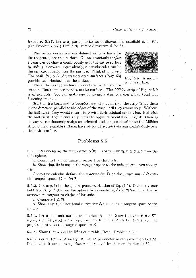
7G C h a p t e r 5: 'L'u e G r a d i e n t

Fig. 5.9: A nonori- entable surface.

E xercise 5.27. Let x(u) parameterize an m-dimeiisional manifold M in (See Problem 4.3.7.) Define the vector derivative d for M .

The vector derivative was defined using a basis for the tangent space to a surface. On an orientable surface a basis can be chosen continuously over the entire surface by sliding it around. Equivalently, a pseudoscalar can be chosen continuously over the surface. Think of a sphere.

■ The basis (x„, x„-} of parameterized surfaces (Page 53) provides an orientation to the surface.

The surfaces that we have encountered so far are orientable. But there are nonoricntable surfaces. The Mobius strip of Figure 5.9

. is an example. You can make one bv giving a strip of paper a half twist and fastening its ends.

S tart with a basis and its pseudoscalar at a point p on the s trip .' Slide them in one direction parallel to the edges of the strip until they return to p. Without the half twist, they would return to p with their original orientation. But with the half twist, they return to p with the opposite orientation. Try it! There is no way to continuously assign an oriented basis or -pseudoscalar to the Mobius strip. Only orientable surfaces have vector derivatives varying continuously over the entire surface.

P roblem s 5.5

5.5.1. Parameterize the unit circle: x($) = cosOi + sinfij, 0 < 8 < 2tt on the unit sphere.

a. Compute the unit tangent vector t to the circle.b. Show that d t is not in the tangent space to the unit sphere, even though

t is.Geometric calculus defines the coderivative D as the projection of d onto

the tangent space: D = P t($ )-

5.5.2. Let 8) be the sphere parameterization of Eq. (1.5). Define a vector field t (4>,8), <fi ^ 0 ,7 r, on the sphere by normalizing dx(<f>,8)/d8. The field is everywhere tangent to circles of latitude.

a. Compute t(0 ,0 ).b. Show th a t the directional derivative c \ t is not in a tangent space to the

sphere.

5.5.3. Let ii be a unit norm al to a surface S in 111'*. Show th a t 0 — n (ri A V). Notice tha t iilf i A x) is tin? rejection of x from n (LAGA Eq. (7.2)), i.e., the

pro jec tion of x on th e ta n g en t space t o S.

5.5.4. Show that a solid in M'5 is orientable. Recall Problem 4.3.5.

5.5.5. Let x : R n —)■ M and y : Rn —> M parameterize the same manifold M.Define what, II: moans to say th a t x and y give I hi' same orientation to Af.

Chapter 6

Extrem a

6.1 E x tre m a

We review four facts about extrema (maxima and minima) of scalar functions on an interval. Have a picture in mind as you read.

® (Extrema) A continuous function / : [a,b] —» R has a maximum and a minimum. A continuous function / : (a, b) —» R need not have a maximum or minimum. Example: f ( x ) = x 3 on ( — 1,1).

e (Local extrema) Let / : (a, b) —» R. Then xo is a local minimum of / if there is a neighborhood jV of xo such that f ( x 0) < f ( x ) for all x G N . And Xo is a local maximum of / if there is a neighborhood N of xo such that f ( x o) > f ( x ) for all x 6 N .

« (First derivative test). Let / : (a, b) —> R. Suppose that f ' ( x ) exists. If / has a local extremum at x, then f ' ( x ) = 0. The converse is not true: f ' ( x ) = 0 does not imply that x is a local extremum. Example: f ( x ) = x 3 on (—1,1) with x = 0.

« (Second derivative test). Let / : (a, b) —> R with f ' ( x ) = 0. Suppose that f " ( x ) exists. If f " (x ) > 0, then f ( x ) is a local minimum of / . If f " ( x ) < 0, then f ( x ) is a local maximum of / . If f " ( x ) = 0, then the test fails. For example, x = 0 is a local minimum of f ( x ) = x A, a local maximum of f ( x ) = — x 4, and neither of / ( x) = x 3.

This section studies analogous facts about extrema of real valued functions defined on subsets of R".

D e fin itio n 6.1 (Bounded set). A set D c R" is bounded if there is a scalar M such th a t (x| < M for all x e D,

So a bounded set is contained in sonic sphere.

T h e o re m 6.2. (Extrema) A continuous scalar valued function defined on a closed and bounded set D C Rn has a minimum value m and a maximum value M in D.

78 C h a p t e r 6: E x t r e m a

A proof is beyond the scope of this text. Both hypotheses, closed and bounded, are necessary for the conclusion of the theorem. For example, consider the scalar function f ( x ) = x. I t has neither a minimum nor a maximum on (0,1), which is bounded but hot closed: And it has neither a minimum nor a maximum on R, which is closed but not bounded.

D efin ition 6 .3 (Local extrema). Let f : U C Rn —» R, where U is open. Then xo is a local minimum of / if there is a neighborhood N of xq such that / (xo) < / ( x ) for all x € N . And xo is a local maximum of / if there is a neighborhood N of xo such th a t /(x o ) > / (x ) for all x £ N .

T h eo rem 6.4 (First derivative test). Let f i U . C R n —>• R , where U is open. Suppose th a t V /(x ) exists. If / has a local extremum at x e U, then V /(x ) =0.

Proof. If x is a local minimum (say) of / , then x is a local minimum of / along all coordinate directions. Thus d ,/(x ) = 0 for all i, i.e., V / (x ) = 0 . □

E x e rc ise .6.1. Let f ( x , y) = x'2 + 2y 2 — x. Find the point(s) where V / = 0.

Second D erivative Test

Let / be a scalar valued function defined on an open set U in R " . If / is differentiable, we gather its first order partial derivatives into the gradient V /(x ) . If / has continuous second order partial derivatives, we gather them into a matrix i? / (x ), called the Hessian matrix:

H f (x) =

'<hif{x) d i2.f (x) ••• 3 m /(x ) '

< W '(X) 922 f ( x ) d2 n f{x )

? n i f ( x ) 5„2 /(x) 9nnf(x)_

(6 .1)

The matrix H f is sjanmetric: 9,;j/(x) = d j i f (x ) (Theorem 3.3). By the spectral theorem, it has an orthonormal basis of eigenvectors {e,-} (LAGA Theorem 9 .23).

The niatrix H f is positive definite if all of its eigenvalues A» are positive. Equivalently, 1) • H f h > 0 for all h 0. This is a. variant of a positive

linear t ransfo rm at ion (LAGA Theorem li.'Sfi and LAGA Defini

t ion

E xerc ise 6.2. a. Expand a vector li = /).;§*. Show that l i - / i /(x )h = Ai/ijf.b. Suppose that H f(x ) is positive definite with smallest eigenvalue A] > 0.

Show th a t h • i?/-(x)h > Ai |h |2.

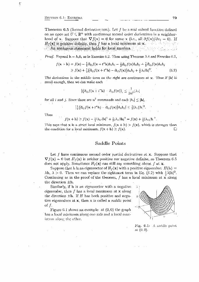
S e c t i o n 6 .1 : E x t r e m a 7 9

T h e o re m 6.5 (Second derivative test). Let / be a real valued function defined on an open set U C R" with continuous second order derivatives in a neighborhood of x. Suppose that V /(x ) = 0 for some x (i.e., all d f ( x ) /d x i = 0). If I I f (x) is positive definite, then / has a local minimum at x.

An analogous statement holds for local maxima.

Proof. Expand h = hi&i as in Exercise 6.2. Then using Theorem 3.4 and Exercise 6.2,

/ (x + h) = /(x) + |<9ij/(x + t*h)hihj - ^dijf(x)hihj + ^dijf(x)hihj

> /(x ) + i ( % / ( x + t* h ) -5 i j /(x ))/li/lj + iA 1 |h |2. (6.2)

The derivatives in the middle term on the right are continuous at x. Thus if |h| is small enough, then we can make each

] (% /(x + /.*h) - <%/(x)) | < 2â|Ai|

for'all i and j. Since there are n2 summands and each |/ij| < |h|,

| i ( a li/ (x + r h ) - a xi/(x ))/ll/l i | < ||A i||h f2.

Thus/(x + h j > /(x ) - | |A , ||h | 2 + ^|Ai||h | 2 = /(x ) + j |A i||h |2.

This says that-x is a strict local minimum, /(x + h) > /(x), which-is stronger than the condition for a local minimum, /(x + h) > /(x). □

Saddle Points

Let / have continuous second order partial derivatives at x. Suppose th a t V /(x ) = 0 but H f(x ) is neither positive nor negative definite, so Theorem 6.5 does not apply. Sometimes H /(x ) can still say something about / a t x.

Suppose that h is an eigenvector of i? /(x ) with a positive eigenvalue: H (h) = Ah, A > 0. Then we can replace the rightmost term in Eq. (6.2) with Â |h|2. Continuing as in the proof of the theorem, / has a local minimum at x along the direction ±h.

Similarly, if h is an eigenvector with a negative i eigenvalue, then / has a local maximum at x along the direction ±h . If H has both positive and nega- o tive eigenvalues at x, then x is called a saddle point of / .

Figure 6 .1 shows an example: at (0,0) the graph has a local minimum along one axis and a local maximum along tlie other.

F ig . 6 .1: A saddle point at (0 ,0).

8 0 C h a p t e r 6: E x t r e m a

E xercise 6.3. Figure 6.1 is the graph of f { x ,y ) = x 2 — y 2.a. Show that V / ( 0 , 0 ) = 0 . ■b. Compute H = H ( f ( 0 , 0 )).c. Show th a t (0,0) is a saddle point of f { x ,y ) .= x 2 — y2,.

E x erc ise .6 .4. Give examples of functions / with H ( f ( 0,0)) = [q §.] and:a. / has a local minimum at (0 , 0 ).b. / lias a local maximum a t (0 , 0 ).c. / has a saddle point a t (0 , 0 ).

The Hessian H j( 0,0) does not distinguish between the three cases in the exercise. For this, we need higher order derivatives. We will not take this up.

There is a simple test for definiteness of a 2 x 2 symmetric matrix..

P r o p o s i t i o n 6 . 6 ^ L e t H = [ $ £ ] b e a ' g e n e r a l 2 x 2 s y m m e t r i c m a t r i x . . T h e n '

, : J ? ,: ' . i s . . p o s i t i v e d e f i n i t e <=> d e t I I > 0 a n d a > 0 ,

II is negative definite <£> dot 11 > 0 and a < 0 .

Proof, We prove the test for positive definiteness. Recall (LAGA Theorem 9.13) and (LAGA Problem 9.2.16) that if A! and A2 are the eigenvalues of II, then

det H = ac — b2 = Ai A2 and tr H = a + c = Ai + A2 .

( = > ) Since H is positive definite, Ai > 0 and A> > 0. Thus det J ? = A1A2 > 0. Then det i f > 0 implies ac > ac — b2 > 0 , so a and c have the same sign. Since a c = Ai -}- A‘2 > 0, a 0.

(<=) det i f > 0 implies A1A2 > 0, so Ai and A2 have the same sign. And (let I I > 0 also implies ac > 0, so a and c have the same sign. Since a > 0, c > 0 also. Now A1 > 0 and A2 > 0 follow from Aj + A2 = a + c > 0. □

E x erc ise 6 .5 . Let f ( x , y ) have continuous second order partial derivatives at (0,0) with df(Q ,0 ) /d x = d f(0 ,G )/dy =. 0 and d e t,///(0 ,0) < 0. Show that (0 , 0 ) is a saddle point of / .

E x erc ise 6 .6 . Find local maxima, local minima, and saddle points of f ( x , y) = x 2 + 2 x y 4- 2 y2 + Ax.

S e c t i o n 6 .1 : E x t r e m a 8 1

P r o b l e m s 6 .1

6.1.1. Let f ( x , y ) = | x 3 4- \ y 2 4- 2xy 4- 5x +.y. Find all local maxima, local minima, and saddle points of / .

6 .1.2 . Let f ( x , y) = x A + y4 — x 2 — y2,a. There are nine points at which V / = 0. Find them.b. Find relative maxima and minima .of / using Theorem 6.5.c. Find the minimum. (Since lim ^^jôo = oo, there is no maximum.)d. Find the saddle points of / using Exercise 6.5.

6.1.3 . L e t'/(x , y) = x2 + j/4 and g(x, y) = x2 ^ j/4. Then V / ( 0 ,0) = V<?(0,0) = 0 and H f ( 0,0) = H g(0,0) - [qq], whose determinant is 0. Despite these equalities, show that (0, 0) is a relative minimum for / and a saddle point for g.

6.1 .4 (Least squares). Given n data points (:ri,j/i), (a>2, 2/2)7 (xn ,yn), the

least squares line, y = nix A- b .minimizes. 'Siijji — (m x i + 6))”. over-all m and b. Use techniques of this section to show th a t m and b are solutions to

mS {Xi n b îUi

This problem vvas solved geometrically in LAGA Problem 4.4.14b.

6.1.5. a. Let duv be the directional derivative dv followed by the directional derivative du. Let / (x ) be scalar valued. Show that duvf = u - i f /(x )v .

b . Show that (?uv = < 9 v u - This is a g e n e r a l i z a t i o n of the equality of mixed partial derivatives (Theorem 3.3). As there, it suffices to prove this for scalar valued / .

From (?h/ = (h • V ) / (Theorem 5.6) we see that the partial derivatives d i f determine, via V , all directional derivatives of / . Part (a) of the exercise shows that the second order partial derivatives d i j f determine, via H f, all second order directional derivatives of / .

82 C h a p t e r 6: E x t r e m a

6.2 C o n s tra in e d E x tre m a

Consider this problem: Find the extreme values of / ( x, y) = x y on the ellipse x 2/8 + y 2/2 — 1. The equation x 2/8 + y2/2 = 1 is called a constraint. You learned one way to solve this problem in scalar calculus: Solve the constraint for y in terms of x (say), substitute the result in x?/8 + y 2/ 2 = 1 giving a function of x only, and set the derivative of the function equal to zero. However, the equations involved are not simple. Moreover, it is often impossible in similar problems to solve the constraint equation for a: or y.

The following theorem provides an alternative, more symmetric, approach.

T h eo rem 6 .7 (Lagrange multipliers). Let / and g be scalar valued functions- defined on an open set U C Rn mid having continuous second order partial derivatives a t xo- Assume th a t V<?(xq) /- 0. If /(x o ) is an extremum of / under the constraint g(x) = c, then '

V /(x o ) = AV5(xo) (6.4)

for some scalar A. The scalar is called a Lagrange multiplier.

The n components of Eq. (6.4) provide n equations in the n + 1 unknowns consisting of the n components of x 0 and the scalar A. Together with g(xo) = c there are n + 1 equations in n + 1 unknowns, which we can hope to solve.

Proof. Let S be the (n — l)-dimensional surface through x» defined implicitly by g(x) = c. (Lemma 5.12). Then Vg(xo) is orthogonal to S at xq (Theorem 5.13).

Let x(£) parameterize S (Lemma 5.12, proof). Then let x(£) = x(£(£)) parameterize a curve on S with x(io) = xq. From Problem 5.2.9,

df(x(t))

dt= ( v / ( x ( o ) - x ,( o ) i t=to.

l=t 0

Since /(x(£)) has an extremum at t = to, the left side is zero. Therefore V /(xo ) is orthogonal to every vector x ; (£q) in the tangent space to S a t xo, i.e., V /(xo ) is orthogonal to the tangent space. Since both V /(x q ) and 'V p(xo) ^ 0 are orthogonal to the tangent space, they are parallel. The theorem follows. □

There is an extension of the theorem to several constraints <7;(x) = a , i =1 , . . . , k. Then a t an extreme point xo there are scalars A* such that

I:V /(x „ ) =: ^ A,V;/,(xu).

1 = 1

I 'he n components of this equation provide n equations in the n + k unknowns consisl ing of the n components of x () and the scalars A,;. Together with </j(xo) = Cj there are n + k equations in n + k unknowns, which we can hope to solve.

There are also extensions of Theorem U.7 to inequality constraints (ji(x) < f , -

S e c t i o n 6 . 2 : C o n s t r a i n e d E x t r e m a 8 3

E xercise 6.7. Find the shortest distance from the plane 3:r — 2y.— z = 3 to the origin. Use Lagrange multipliers. Hint: It is easiest to find first the square of the minimum distance. Ans. 3 / \ /l4 .

Suppose th a t we want to find the maximum or minimum of / on a set B U U in R” consisting of an open bounded set U and its boundary B. The next exercise shows one way to proceed.

E x erc ise 6.8. Find the maximum and minimum values of f ( x , y ) = xy in the region x 2/ S .+ y2/ 2 < 1. Here U consists of points with x 2/8 + y2/ 2 < 1 and B points with x 2/S + y2/ 2 = 1.

a. Find points in U with V / = 0. This gives candidate extreme points in U (Theorem 6.4).

■ b. Find points in 13-with V / (x ) = AVg(x), where g(x ,y) = x 2/8 + y2/2. ■This gives candidate extreme points in B (discussion following Theorem-6.7).

c. The extreme values of / in B U U are among the candidates from Parts (a) and -(b). Evaluate / at .these points and choose -the extrema.

T h e o re m 6.’8 (Interpretation of A). Let / and g be a.s in Theorem 6.7. Let c range over an open interval in the constraint y(x) — c. Suppose th a t for each c there is a unique maximum M(c) of / a t x 0(c). If x^(c) exists, then so does M '(c), and M '(c) =:A.

Proof. Differentiate ff(xo) = c with respect to c: V<?(x0) • x(> = 1 (Problem 5.2.9). Now compute:

M'(e) = £ ; / (x o ( f ) ) = V / ( x 0) • Xq = AVs(x0) - x[, = A. □

E x erc ise 6 .9 . Let f ( x , y ) = xy and g(x ,y) = 2x + 2y.a. Show th a t the maximum of / subject to g(x, y) = 20 is 52, with Lagrange

multiplier A = 2.5. The maximum of / subject to g(x, y) = 21 is (5.25)2.b. Approximate M ' and show that this is in accord with Theorem 6.8.c. Compute M(c) exactly, then M'(c). Compare with Part (b).

Problem s 6.2

6.2.1. Find the shortest distance from the hyperbola x 2 + Sxy + 7y2 =■ 225 to the origin. Proceed as follows. It is easier to solve for the square of the shortest distance. Write Eq. (6.4) as a pair of homogeneous linear equations in x and y, where the coefficients depend on A. It is clear geometrically that this problem lias a solution. And it is clear that (0,0) is not a solution. Thus the linear equations have a solution other than (0,0). From LAGA Theorem 3.16 and LAGA Theorem 8.24, the determinant of the coefficient matrix is therefore zero. This gives two A’s. Only one of them is suitable. Ans. 5.

8 4 C h a p t e r . 6: E x t r e m a

6.2.2. In many applications it is of interest to find the largest, dr largest few, eigenvalues of a large symmetric matrix A. Examples include the singular value decomposition (LAGA Section 9.7) and principal component analysis (LAGA Problem 9.4.10). Show that the largest eigenvalue occurs at the maximum of x- A x on the unit sphere |x| = 1. (According to Theorem 6.2 the maximum exists.) Hint : |x| = 1 is'the same as |x |2 = 1.

6.2.3. Find the maximum and minimum value of f ( x , y) — x 2 — xy + y 2 + 4 on the triangle with edges x = 0, y = 4, and y = x. Ans. Max 28, Min 4.

6.2.4 (Maximum entropy). The probability of any given face turning up on a toss of a fair die is | . Thus if we toss the die many times, then the average number of spots on the top face is about

.. . l x i + 2 x § + 3 x | + 4 x i + 5 x i + 6 x | = £ t i * i

The sum is 3.5 (half way between 1 and 6), as you can check.Now suppose th a t someone tosses a die many times and reports an average

of 4.5. Then Yfi=i iPi = 4.5, where pi is the probability that face i is on top. What are these probabilities? Many sets of probabilities have a 4.5 average, so there is no answer without further guidance.

There are many reasons to call — Y f i P i ^ P i 1 the uncertainty (or entropy) of the probabilities. We do not go into this, but we reformulate the question: If J2t=i^Pi = 4-5, what probabilities p.; give the maximum uncertainty? We are invoking the principle o f maximum uncertainty (or entropy) to solve our problem.

a. Express the problem as a Lagrangian multiplier problem. (The constraints pi > 0 need not be included, as they will turn out to be satis’fied in the solution.)

b. Write equation Eq. (6.4) for this problem.c. Solve your answer to Part (b) for the p-i in terms of A.

d. Your answer to Part (c) does not require that Y ^ P i W = 1- Impose that condition to obtain probabilities pi which sum to 1.

Solving J2i=i i P i W ~ 4.5 numerically for A gives the increasing probabilities

pi = .055, p2 = .079, p3 = .114, P4 = .165, p5 = .240, p6 = .347.

Solving the same problem for an average of 3.5 (expected for a fair die) gives all P i — 1 /6. Solving for an average of 2.5 gives the probabilities above reversed.

6.2.5. Suppose {.hat we know n oth ing about a probability distribution p i , p2, . • •, ]>,i other than Vi ~ 1- Intuitively, we assign equal valuesp i = J fit. for all i. Show that the principle of maximum uncertainty also does this.

1 Since /),. < J , In?),; < 0: h en ce th e ” , A nd we define 0 I n 0 = linix -+o x Imc = 0.

Part III

In tegrals

C hapter 7

Integrals over Curves

7.1 T h e Scalar In teg ra l

Define d x

Before studying integrals over curves, the topic of this chapter, we'review the def- • inite integral f dx from scalar calculus. One interpretation of the integral is the area of the region under the graph of y = f ( x ) between x = a and x — b. If / were constant between a and b, say f ( x ) — h, then the region is a rectangle with area equal to height x base: h(b — a).'

This not being the case in general, we approximate the area under the curve with the sum of areas of rectangles. See Figure 7.1.

d ---X q X1 x% b=x*

Region under the curve approximated by three

Fig. 7.1:y = /(z)rectangles.

If we nse more and more rectangles with narrower and narrower widths, we more closely approximate the area. In the limit, we obtain the area.

Here are the details. A partition of the interval [a, 6] is a set of points

P = {.t0 = a, a-i, . . . . 'xn = 5}

with xo < Xj < ■ ■ ■ < xn . Given P, choose points X*,X2 , .. • ,x* with i < x^ < x^, 1 < i < n. In Figure 7.1, n — 3. Now set = Xi — X i^ i , i = 1 . , n and form

(7,1)

This Iliemann sum is the suiii of the areas of the rectangles. It is an. approximation to the area under the curve. We now take a limit to get the exact area.

8 8 C h a p t e r 7: In t e g r a l s o v e r C u r v e s

D e f i n i t i o n 7.1 (Scalar integral: f dx). Define the norm |P | of a. partition P of [a, ii] to b e the maximum of the lengths A iX. Then the (definite) scalar integral of / over the interval [a , fa] is

f f d x = lim j r f { x * ) A i X , (7.2)

provided th a t the limit exists.

If dx exists, then we say th a t / is integrablc on [a, b\.

Say th a t / is bounded on [a, b] if there is a constant M so that |/(x')l ^ M for all x, a < x < b. Geometrically, the graph of / can be enclosed between horizontal.lines, one above the. graph and one below.

We state the following theorem without proof.

T h eo rem 7.2 (Existence' of f dx). Let / .b e a bounded function on an interval [a, 6] and continuous there except perhaps for a finite number of points.

Then f ' ’ f dx exists.

A continuous function on a finite interval [a, 6] is bounded (Theorem 6.2) and so is i n t e g r a b l e there.

E xercise 7.1. Define the function f ( x ) = x sin ~F for x / 0 and /(0 ) = 0. The graph of / oscillates between —x and x infinitely many times near x 0. See Fig. 7.2. Show that nevertheless l f dx exists.

E xerc ise 7.2. Define

0, if x £ [0,1] is rational

1, if x 6 [0,1] is irrational.

Show th a t / * / dx does not exist. To solve this exercise you need only know that there are infinitely many rational numbers and infinitely many irrational numbers in every interval of R.

Then* are many other interpretations of the scalar integral beside areas. For example, suppose that a wire is laid on \a,b) with mass density p = p(x), measured. say. in grams/em. If p were const,ant between a and b, say p(x) = po, (lien the mass would be density x length: m — />,,(& — a), in grams.’

This not being the case in general, we approximate the mass with the sum of small masses, as in Eq. (7.1), (with p replacing / ) and take a limit as \P\ —> 0.

Then (die mass of the wire is m = / * pdx, in grams.

F ig . 7 .2 : The graph ofxsin(‘2ir/x).

S e c t i o n 7 . 1 : T h e S c a l a r I n t e g r a l 8 9

C om pu te J 6 f dx

Equation (7.2) tells us what f ^ f d x is. W hat about computing it?

T h e o r e m 7 . 3 ( F u n d a m e n t a l t h e o r e m o f c a l c u l u s , I ) . S u p p o s e t h a t F' e x i s t s

o n ( a , 6 ) , a n d i s c o n t i n u o u s o n [a, b\. T h e n F'dx — F(b) — F(a).

The function F is an indefinite integral, or antiderivative, of F ' . The theorem

expresses a definite integral F 'dx in terms of an indefinite integral F.The theorem is stated in a slightly different way than usual. Usually we are

given a continuous function f on (a, b) and want to compute f b f ( x ) dx, If we

can find an F with F' = f , then f d f ( x ) d x = F(b) — F(a). Our formulation will allow easy comparison to a huge generalization, the Fundamental Theorem of Geometric Calculus (Theorem 10.1). • • .

Proof. F ( b ) - F ( a ) =

(F (xn) - F (xn- 1)) + (F (xn - i ) ~ F (x n- 2)) + • - ■ + (F (x 1) - F (x 0))

= F ' ( i ; _ 1)An_ ix + n < _ 2)A „_2a: + F'(x*0)A 0x ,

lP ° f bF ’dx: . v .J a

All terms of the telescoping sum on the right side of Step (1) cancel except F (x n) = F(b) and —F (x 0) = —F (a ). Step (2) uses the scalar mean value

theorem (Problem 3.1.2). The last step is Definition 7.1 of JaV dx. □

One way to think about the theorem is th a t the integral f ^ F ' ( x ) d x adds infinitesimal increments dF = F '( x )d x of F to obtain the entire increment F(b) — F(a).. (See the next page about using infinitesimals.)

T h fo ro m 7 A (Fundamental 11icorem of calculus, Tl). Suppose that / is continuous iu Set F[x) -- J ' f (1)di . Then F is an iini.iderivaiive of / : F 'ix ) - S ix).

This existence theorem for antiderivatives, which we do not prove, does not give a formula for the antiderivative in order to apply Theorem 7.3.1 This is often impossible. Then we must use numerical techniques.

Computers can approximate definite integrals using Eq. (7.2) with partitions of small norm, or by using more sophisticated versions of the sum. Perhaps you know of the trapezoidal rule or Simpson’s rule.

Please be clear about the difference between:

• W hat the integral is: A number, the limit of sums (Definition 7.1). The number can represent areas, masses, etc.

« Computing the integral: Use an antiderivative (a function) or a computer.

lrThe W olfram M athematica Online Integrator is an a m a z in g on line resource for find ing antiderivatives ( h t t p : / / i n t e g r a l s . wolf ram. com/index, jsp ) .

90 C h a p t e r 7: In t e g r a l s o v e r C u r v e s

H ow to T hink about an Integral

We will encounter several kinds of integrals in Part III of this book. Let us use the integral fa f dx to discuss an intuitive way to think about them. This will not be a rigorous discus

sion of f dx\ we have already taken care of that. We, together with most people' who use calculus, will use the language of infinitesimals.

There are no infinitesimals .among the real numbers, . Nevertheless, they are very useful j ' ^rtoftotegralwhen thinking about integrals. Interval over

Refer to Figure 7.3. The integral is written which integral i[a 6] f dx there ^0 conform to the notation for is talcen

generalizations of the integral. Fig. 7.3: The anatomy qf an

[a, b]. This interval is the object over which the integral.integral is taken. The integral obeys these rules: -

I a f dx = a I f dx, I ( f + q ) d x = f dx + I gdx.J{a,b] J\a,b] . J[a,b] J [a,b] . . J[a,b]' .

We will study integrals over curves, surfaces, and solids, and replace [a, 6] with the curve, surface, or solid. Analogs of these rules will remain true.

f. This is the integrand, tlie function to be integrated. It must be defined on the interval [a, b]. We often leave off its argument, “x ” in this case, when not needed for clarity. For integrals over curves, surfaces, and solids, / must be defined on the curve, surface, or solid.

dx. This is the length of an infinitesimal part of [a, 6], For integrals over curves, surfaces, and solids, dx is be replaced with the infinitesimal length ds, area dA, or volume dV of an infinitesimal part of the curve, surface, or solid.

f dx. This is an infinitesimal part of the integral. We have seen the examples of an infinitesimal area / dx and an infinitesimal mass p dx. For integrals over curves, surfaces, and solids, f ds, f dA, and f d V represent infinitesimal parts of the integral. For example, pds, pdA, and p d V represent the infinitesimal mass of an infinitesimal part of a curve, surface,' or solid.

/ . The integral “adds up” the infinitely many infinitesimal parts f dx of the integral to obtain a whole, /jo / dx. We have seen the examples of adding up the areas of infinitely many infinitesimal rectangles and the masses of infinitely many infinitesimal lengths.

For integrals over curves, surfaces', and solids, the integral adds up the infinitely many infinitesimal parts of the integral. For example, fc pds, f j ^ p d S , I f fy p d V are the masses of a curve, surface, and solid, respectively. The number of integral signs J tells us the dimension of the object over which the integral is taken.

Similar descriptions apply to integrals over manifolds (Section LA).

Adds up the infinitesimal parts / dx Function

defined on [a,6]

ffdx, J '-r-J

laM \

Length of " infinitesimal

part of [a,b]

S e c t i o n 7 .2 : T h e P a t h I n t e g r a l - 9 1

7.2 T h e P a th In teg ra l

The path integral integrates fields defined on curves (paths).2

D efin itio n 7.5 (Path integral: Jc F d s) . Let F be a field on a curvc G in Mn . Parameterize C: x: [a, b] —> R” (Eq. (1.2)). Then the path integral of F along C is defined bv"

(7:3)f F d s — f F(x(t)) \x '( t ) \d t . J c j[a,b]

“Tin; into/r.iiid on tin- is multivector valued, but the integral is still defined byKd. IV.S).

We give an “infinitesimal understanding” of Eq. (7.3). On the left side, ds is the length of an infinitesimal piece of C. Multiply it by the value of F at some point in the piece to give F ds, an infinitesimal piece of the integral.

Nowt/x

ds = |x(( + dt) — x(t.) | =dt

dt = |x'(i)|dt, (7.4)

i.e., |x '( i) | is the “infinitesimal magnification factor” of x. Multiply by F: F d s — F.\x'(t)\dt. Sum (integrate) to obtain Eq, (7.3).

E xerc ise 7.3. Let C be the first quadrant portion of the circle of radius 2 centered at the origin and oriented clockwise- Evaluate f c y ds. Ans. 4.

If a wire of density y in grams/cm is laid on C, then the integral gives its mass in grams.

E x erc ise 7.4. a. Let C be a curve in the xy-plane with a J___“ribbon” of varying height li(x, y) above it. See Figure 7.4. S Express the area of the ribbon as a path integral. ^

b. Compute the lateral area of the cylinder of Figure 1.8 rinsing the integral of Part (a). F ig . 7.4: A ribbon

T h e o re m 7.6 (Path integral properties). If the integral(s) below on the right exist, then so does the integral on the left, and equality holds.a. f c c F d s = c f c F ds.

b. U F + G) d s = L F d s + L G ds.

°-'lcluc>Fds = fclFds + fclFds,where the terminal point of Cj is the initial point of C%.

Proof, a. f cp d s = f c F ( x ) |x '| dt = c f F ( x ) |x'| d t = c f J c J{a,h] J_[a,b] ■ J c

Step (2) uses the analogous property of scalar integrals.Problems 7.2.5 and .7.2.6 ask you to prove Parts (b) and (c).

F d s .

□2N a m e s o f th e in tegra ls o f th is c h a p te r a n d C h a p te r 9 vary am o n g au th o rs .

92 C h a p t e r 7: In t e g r a l s o v e r C u r v e s

Sometimes a curve C is parameterized differently on different sections. For example, C might be a closed curve consisting of a semicircle and the diameter connecting its endpoints. By Part (c) we can integrate over each section and then add to get the entire integral.

We will encounter several more integrals in this book. To be worthy of the name, they must satisfy Parts (a)-(c) of the theorem. .

E xercise 7.5. Suppose that the helix of Figure 1.3 has mass density p(x(0))0~. Find the mass of the helix. A tm, (67t)3\/2/3.

Let x(i) = x(t)i + y(t)j parameterize a curve in K2. Express Eq. (7.3) in ' terms of x(t) and y(t):

Here is an easy algebraic way to remember/understand the ds part of this formula:

[ F ( x ( t ) ) d s ~ I F (x(t) , y(t)) \ f x ' 2{t) + yr2(t}dl. (7.5)J c J[a,b\

ds2 = dx2 4; dy2 = ^ 0 df2 = (x ' 2(t ) + y '2(0 ) d t‘2- (7-6)

Of course there is a 3D version of this.

S e c t i o n 7 . 2 : T h e P a t h I n t e g r a l 9 3

A rcleng th

Set F = 1 in Definition 7.5. Then we have the arclength, or simply length, of C:

i(C) = I d s = f |x'(i)| dt. (7.7). JC J[a,b]

If t is time, then the formula says that the distance traveled along C is the integral of the speed |x /(£)| over [a, b].

E x e rc is e .7.6. Compute the length of the helix of Figure 1.3. Ans. 6\/2tt.

The length of the curve from x(a) to x(t) is

s(t) = [ '•|x '(r)|'dr = f |x '(r) | dr. /J \a , t \ J a

If |x '| is continuous, then (fundamental theorem of scalar calculus)and / 0 (Page 48). By the scalar inverse function theorem (Section 3.6) the function s = s(t) lias an inverse function t = t(s). Then x(s) = x(t(s)) parameterizes the curve with its arclength s, i.e., x(£(s)) is a t ‘distance s from x(a) along C. . .

This is an important parameterization, as it simplifies many expressions. Theorem 7.7 will provide our first example.

E x erc ise 7.7. Reparameterize the circle of radius r of Figure 1.1 .with arclength. Hint: 6 = s / r is the definition of radian measure.

E x erc ise 7.8. Consider the helix x(6) = rcosOl + rsin#j + hdk, 9 > 0. The constant h is called the pitch of the helix. The larger h is, the faster the helix climbs. Figure 1.3 is the special case r = h — 1. Set v =■ y/r2 + h'2.

a. Find s($).b. Find 8(s),c. Parameterize the helix in terms of s.d. Compute d and show th a t it has norm 1.e. Solve Exercise 7.5 again using s as parameter.

T h e o re m 7.7. Parameterize a curve with arclength: x(s). Then = t , the unit tangent vector to the curve.

Exercise 7.8d is an example.

Proof. From above, | dx / dt | = d s /d t . Thus

( dx /d t d x /d t dx

\d,x/dl\ ds/dt ds '

The equation shows that parameterizations not using s have more complicated derivatives: = ^ ft. • ■

9 4 C i i a p t k r 7: In t e g r a l s o v k r O u rv rs

P roblem s 7.2

7.2.1. Suppose that a wire lying along a curve C is contained in a region with a temperature field T. Express the average temperature of the wire. Recall that

the average of a scalar function y = f ( x ) on an interval [a, 6] is f dx/(b — a).

7.2.2. a. Let r = r(t), 6 = 8(t), z = z(t), a < t < b parameterize a curve C in cylindrical coordinates. Show that

I ' F ( f , -0 ,z )d s= f F(r, d, z) \Jr’2 4- r 2 Ba 4- z '2 dt.' ■ ! ( ■ J[a,b] ■ . ’ • •

The corresponding result, for spherical coordinates is

■ f F(p, 6,8) ds = I F(p, (b, 8) J p'2 4- p2(j>12 + p2 sin20 8'2 dt:■ ! ( ■ J f a , 6] ■ . . . •

b. Compute the length of the curve r = et, 8 = t, z = el , 0 < t ■< 1. Ans. \/3(e - 1).

7.2.3. Parameterize a curve in R2 in polar coordinates: r(8), a < 8 < b. Show that its length is 6j \Zr'2 + 'r2d8.

7.2.4. a. The graph of the scalar function y = f ( x ) , a < x < b can' be .parameterized x ( . t ) = x i4 - /(x ) j , a < x < b: Show that the length o f the graph is /jofcj i / l + f ' 2 dx. Perhaps you saw this formula in your scalar calculus class.

I). Make a calculation similar to Eq. (7.(!) to help remember the formula.

7.2.5. Prove Theorem 7.6b.

7.2.6. Prove Theorem 7.6c.

7.2.7. Let S be a surface in M3 parameterized by x(ui,u-2). Let C be a curve in S parameterized by x (« i( i) , u-2(t)), a < t < b. Show th a t the length of C is

s = [ J (xj - x-jlUiUj dt, ' (7.8). J{a,b] V

the curve, «^(f)u'-(i). The matrix is called the metric.o( the.

The formula separates properties of the surface, x;(t) • Xj(t), from those ofX j - X j X j - X 2

X2 • X] x 2 • X9surface. We will have more to say about the metric in Chapter 11.

7.2.8 (Shortest path). Let x ( t )-parameterize a curve in M” with x(a) — p and x(6) = q. Let v be a constant vector with |v| = 1.

a. Show that (q — p) - v — f* x '(t) - v dl < f* |x '(f)| dt. Hint:' First show that (x(t) • v ) ' = x'(t) • v.

b. 'Fake v = an(i show that jq — p| < |x'(/,)| dl. Since the inequality

is Jess than or equal, this says that the straight, line between p and q is a shortest path from p to q. It does not say that it. is Hie only shortest path. (But it is.)

S e c t i o n 7 .3 : T h e L i n e I n t e g r a l 9 5

7.3 T he Line In teg ra l

The line integral is a second integral lor fields defined on curves in R n.

D e f i n i t i o n 7 . 8 ( L i n e i n t e g r a l : Jc F ds) . L e i F b e a f i e l d o n a n o r i e n t e d c u r v e

C i n R” . P a r a m e t e r i z e C: x(t) , a < t <b. T h e n t h e line integral o f F a l o n g C

f F d s — f F(x(t)) x '( t) dt. (7.9)J c J[a,b\

T h e i n f i n i t e s i m a l v e c t o r d s = t ds, w h e r e t i s a u n i t p s e u d o s c a l a r i n t h e t a n g e n t

l i n e t o S . ( a u n i t v e c t o r t a n g e n t t o C) a n d o r i e n t e d w i t h i t .

We can see Eq. (7,9) in infinitesimal terms:

ds = t ds = ^ / ( ^ l lx /^ l ^ ’ (7-10)

Step (2) uses the fact th a t x '(i) is tangent to C and also Eq. (7.4).

E x e r c i s e 7.9. a. If / is a scalar field, then Jc f ds is a ____________Choosefrom scalar, vector, bivector.

b. If f is a vector field, then fc f ds is a _____ _

E x erc ise 7.10. Parameterize a curve C from a to b by x(/,),' a < t < b. Show th a t Jc ds = b — a. Hint: Use Definitions 7.8 and 7.5.

E x erc ise 7.11. Let C be the unit circle, oriented counterclockwise. Let f be a constant vector field on C. Determine Jc f ds using the language o f infinitesimals. Hint: Look at diametrically opposite points.

E x e r c i s e 7.12. Compute Jc fd s , where f ( x i + yj) = 2xyi + y2j and C is the straight line from (0,0) to (1,2). Hint: First parameterize C as x(t). For this, recall Exercise 1.6. Then substitute into f(x(t)). Ans. 4 + | i j .

T h e o r e m 7 . 9 ( L i n e i n t e g r a l p r o p e r t i e s ) . I f t h e i n t e g r a l ( s ) b e l o w o n t h e r i g i i t

e x i s t , t h e n s o d o e s t h e i n t e g r a l o n t h e l e f t , a n d e q u a l i t y h o l d s .

a. fc c F d s = c.jc Fds.

b . j c (F + G) ds = j c Fds + f c G ds.

c- icy jca F d s = f c , F ds + i c 2 F d s >where the terminal point of C\ is the initial point; of Co.

Proof. Since the line integral is defined in terms of a scalar integral, the line integral inherits these properties from the scalar integral. Exercise 7.13 asks yon to show this explicitly for Pari, (a). □

E x erc ise 7.13. Prove Theorem 7.9a.

96 C h a p t e r 7: In t e g r a l s o v e r C u r v es

Just as the gradient of a vector field can be split into its divergence and curl, the line integral of a vector field can be split into two pieces.

E xercise 7 . 1 4 . a. Let f be a vector field. Define f c f • ds and j c f A ds.

b. Show that I f ds = / f • ds +J c J c

c. Let C be a curve from a to b. Show that f c x • ds = | ( b 2 — a 2).

E x e r c i s e 7 . 1 5 . Let C be the unit circle, oriented counterclockwise, and f = — yi + xj be a vector field on C. Determine j c f • ds using the language of infinitesimals. Hint: f is tangent to C. Ans. 2ir.

E x erc ise 7 . 1 6 . Let f(x) = 2i. Put. in. numeric order the integrals f c f • ds , Jc f • ds, f c > f - ds in Figure 7.5. .

In applications f c f - ds is the most common line integral. We give, two physical interpretations: work and circulation.

W o rk . If a constant force f acts on an object constrained to move along a ' straight line through a displacement A s , then' the work done on the object by .that force is w = f • A s . Thus if f acts parallel to the line in the same direction as A s , then w = | f | | A s | . If f . acts perpendicular to the line, then w = 0 . 3 If the object moves on a curve G, then the work is defined (of course) as

w = j f -d s . (7.11)

E x erc ise 7 . 1 7 . Find the work done by the force i'(x, y, z) = yi — xj + z~k in moving an object along the helix of Figure 1.3. Ans. — 6tt 4- (6tt)3/3.

C ircu la tio n . If C is a closed curve, then f c f • ds is called the circulation of f around C. The expression |f |eos# is the length of the component of f along (parallel to, not across) C.See Figure 7.6. Thus f • ds = ( |f |co s0 ) \ds) is just what.you might want to call part of the circulation of f around G. ,

For a physical example, let f = v, the velocity field of a gas f for liquid (i.e., a fluid) flowing near C. The circulation Jc V 'ds around C ~ is fundamental in the study of fluids. f c f-ds.

E xercise 7 . 1 8 . If C is the rim of a water wheel, with very many very small vanes attached, then the circulation j c v ■ ds is a measure of the total force imparted to the wheel. '

a. Suppose; that for a water wheel v • ds < 0. with the integral taken counterclockwise. Wliat will the wheel do?

b. Suppose that v is a. constant, the same everywhere around the wheel. W hat will the wheel do?

* >Cl

/ *c 2

Fig. 7.5

/ f A ds, scalar + bivector. J c

3T h is is d i f fe r e n t f r o m e v e ry d a y usage . W o r k as d e f in e d h e re here re q u ire s b o th a fo rce

a nd m o t io n . I f von push o n an n o M in i fc r h ow h a rd a n d h o w lon g , a n d i l d ocs nol.

niuv'i.1. U km ) y o u in ive d o n e no w o r k o n th e ob jco l..

S e c t i o n 7 .3 : T h e L i n e I n t e g r a l 9 7

Next is a standard formula tor computing the integral fr f • ds. Let;

f (z, V,z ) = /(■'<■’, y, z)i + g(x, y, z)j h(x, y. z )k.

Parameterize C: x ( t ) — x ( t )i + y(t)j + z(t)k, a < t < b. Then

f f • ds = f f ( x ( t ) ) - x ' ( t ) d t J C J[a,b]

= [ ( f i + 9 1 + hk) * ( x ' i + y'j + z ' k ) dt. . . . / [ a, 6] ' ■ ' '

= f { fx ' -f gy' + h z ) dt.J [a,6] . . , •

This is usually written . ■

j i • ds = J f dx + gdy 4- h dz , (7.1.2)

where for computation on the right,

f d x = f (x ( t ) , y(t), z ( t))x '( t )d t , etc. ■

•Equation (7.12) is our formula.

E x e r c i s e 7 . 1 9 . Solve Exercise 7.17 again-using Eq. (7.12).

The next theorem generalizes the fundamental theorem of scalar calculus, f ^ F 'd x = F(b) — F(a) (Theorem 7.3).

T h e o r e m 7 . . 1 0 . Lei. o(~x) b e a d i f f e r e n t i a b l e s c a l a r f i e l d o n a n o p e n s e t U C M n .

I f C i s a p a t h i n L! f r o m x j t o X 2 , t h e n

f V 0 .d s = tf(x2) - 0 ( x i ). (7.13)J c

Proof. Parameterize C with x(i). Then

f V4>-ds= f -x 'd t = f (<f>ox)'dtJ C J[a M

= ( < ^ o x ) ( 6 ) - ( 0 o x ) ( a ) = <p(x2) - 4>(xi).

Step (1) is the scalar part of Definition 7.8. Step (2) is Problem 5.2.9. Step (3) is the fundamental theorem of scalar calculus (Theorem 7.3). □

E x e r c i s e 7 . 2 0 . Let f (x ,y) = yi + x]. Determine Jc f • ds, where C is a curve from (1,1).to (2,-2). Ans. 3.

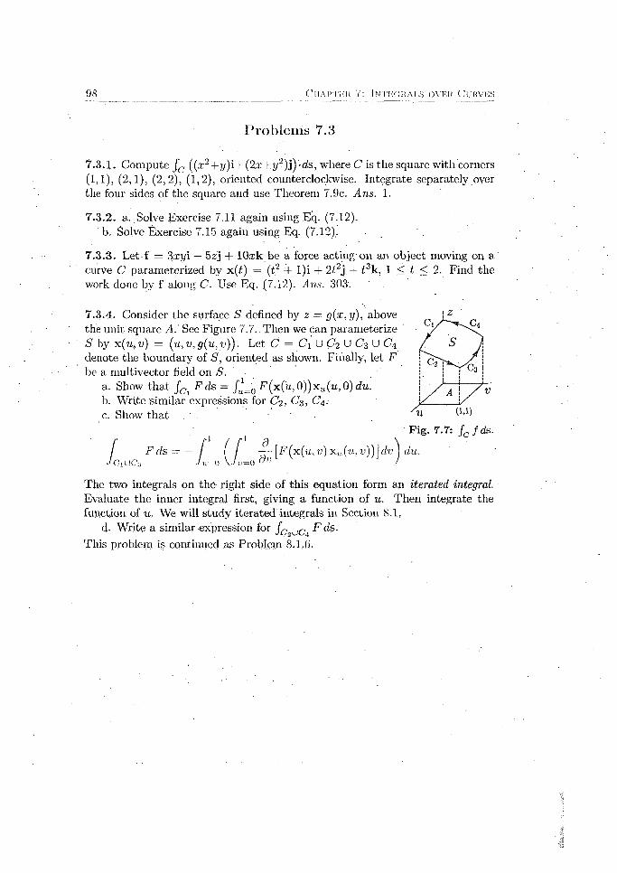
98 ( ■ H A r r e n 7: In t e g r a l s ovicr O urvks

Problem s 7.3

7.3.1. Compute f c ((x2+2/)i+(2a:4T2/2)j) -ds, where C is the square with corners (1,1), (2,1), (2,2), (1,2), oriented counterclockwise. Integrate separately over the four sides of the square and use Theorem 7.9c. Ans. 1.

7.3.2. a. Solve Exercise 7.11 again using Eq. (7.12).b. Solve Exercise 7.15 again using Eq. (7.12),. -

7.3.3. Let f = 3,xyi — 5zj + 1 0 ik be a force actingon an object moving on a curve C parameterized by x(t) = (t2 + l)i + 2i2j + t 3k, 1 < t < 2. Find the work done by f along C. Use Eq. (7.12). Ans. 303'. ' .

7.3.4. Consider the surface S defined by z = g(x ,y) , above the unit square A.' See Figure 7.7..Then we Can parameterize S by x(u, v) = (u, v, g(u,v)). Let C = C\ U C2 U C3 U C4

denote the boundary of S, oriented as shown. Finally, let F be a multivector field on S.

a. Show that f Cj F d s = F ( x ( u , 0 ) ) x u ( m , 0 ) du.b. Write similar expressions for C 2 , C 3 , 6 4 .c. Show th a t '

F d s =CjuC’3 u.= 0

JL„ d v

[F(x(u,t>)x„(u,t'))]fit

The two integrals on the right side of this equation form an iterated integral. Evaluate the inner integral first, giving a function of u. Then integrate the function of u. We will study iterated integrals in Section 8.1.

d. Write a similar expression for f c 2u c4 F ds-

This problem is continued as Problem 8.1.6.

S e c t i o n 7 .4 : C o n s e r v a t i v e V e c t o r F ie l d s 9 9

7.4 C onserva tive V ector F ields

P ath Independence

A parameterization x(t), a < t < b, of a curve C gives an orientation to C: start at x(a) when t — a and traverse the curve with t to x(6) when t = b. The parametrization x (a + b — t), a < t < b also parameterizes C, but gives it the opposite orientation: when t = a, x (a + b — t) = x(6) and when t = b, x (a + b — t) = x(a). Denote opposite orientations of a curve by C and —C.

Path and line integrals behave differently under a change of orientation:

/ / ds = / f ds and-c . Jc

f f ds = — f f ds.J - c J c

The reason is th a t ds, a length, is unchanged with a change of orientation j whereas ds, a vector, reverses sign with a change of orientation. .

Consider now two curves, C\ and C'2, between the same two points. See Figure 7.8. We ask the question of path independence: Is f c f • ds = f c f • ds? This'fails in general but holds for the very important class of conservative vector fields, the topic of this section.

There is a trivial but useful criterion for path independence. A curve is closed if its initial and terminal points are the same.4 Thus C 1U—C2 is a closed curve: start a,t x i, traverse C \ to x-?, and traverse —Co from x2 back to Xj.The criterion is th a t the integral around the closed path Ci U — C2 is zero:

Fig.Twofrom

7 .8 :

paths X l tO X ‘2-

[ f • ds = f iJ Ci J C2

f * dsJc

f - ds = 0.C iU — C 2

(The symbol (f is often used to denote an integral around a closed curve.) To see this, compute:

j f ■ ds - j f ■ ds = j f ■ ds + j f • ds = <£ f -ds.JC) Jc> Jci J-C2 / c , u - c 2

The left side is zero if and only if the right side is zero.

'’T h is is d ifferent from th e closed se ts of Definition 2.4.

1 0 0 C h a p t e r 7: In t e g r a l s o v e r C u r v es

C onservative Vector Fields

D efin ition 7.11 (Conservative vector field). Let f be a vector field on an open set U. If there is a scalar field <fi with V</; = f, then f is conservative on U.

The field <p is called a (scalar) potential for f .

A potential is analogous to an antiderivative in scalar calculus. However, in

The first theorem is an immediate consequence of Theorem 7.10.

T h e o re m 7.12. If f is a conservative vector field in an open set U in R” , then line integrals of f-in-t/ are .independent -of path:

a. Use Theorem 7.12. Find <j> by inspection.b. Use Eq. (7.12) to compute th e integral over the line from (0,0) to (1,2).

The second theorem is the converse of Theorem 7.12.

T h e o re m 7.13. If line integrals of f in an open set 1/ in R" are independent of path, then f is conservative.

Proof. For ease of notation we take n = 2, so f = / i + gj.Fix a point xq = (xo,yo) 6 U and define the scalar field

path taken from xq to x. We will show that d ^ /d x = f .Similarly, d<p/dy = g. This establishes the result.

Let x = (x,y). Since U is open, there is a point (£, y) with FlS- 7-9: 1 he £ < x such that the horizontal line segment from (£, y) to •S0Kment is >n V. (x, y) is in U. See Figure 7.9. Parameterize the segment x(t) = ti+ i/j, (, < t < x. Then x'(t)dt = idt.

The first integral is independent of x. Thus differentiating the, right side with respect to x holding y fixed gives ' -

Mn a potential need not exist. The next two theorems show that a vector field is conservative if and only if its line integrals are independent of path..

E xerc ise 7.21. Compute- f ^ ' ^ ( 2 x y 2i + 2x2yj) • ds in two ways. Ans. 4.

0(x) = f • ds. Bv hypothesis, 0(x) is independent of the

Express y) i - d s + f • ds.

Stop (3) uses the fundamental theorem of scalar calculus (Theorem 7.4). □

S e c t i o n 7 .4 : C o n s e r v a t i v e V e c t o r F i el d s 1 0 1

The most; important conservative tick) is in R'!: f(x) = - -x / |x |3. It is antiparallel to x and inverse square: |f(x)| = l / |x |2. Figure 7.10 depicts the field in K2.

The Newtonian gravitational force and the Coulomb electric force (multiplied by suitable scalar constants) are given by this f. Exercise 5.6c shows that V ( l / |x |) = —x / |x |3. In other words, l / |x | is a potential for —x / |x |3.

E x erc ise 7.22. C o m p u t e —

Ans.

E x erc ise 7.23. Use spherical coordinates to prove again that V ( l / |x |) = —x / |x |3.

V A f — 0

We turn to a second, more useful, characterization of conservative vector fields. The next theorem is an immediate consequence of Theorem 5.9ai

T h e o re m 7.14. Let f be a continuously differentiable vector field on an open set U in Kn . If f:is conservative, then V A f = 0. (In R3: V x f = 0.)

The converse of Theorem 7.14 is not true: a vector field with zero curl need not be conservative. Here is the example everyone uses.

—yE x erc ise 7.24. Let f (x ,y) = ----- î H— =----- ^j.x + 3/ x + y

a. Show th a t V A f = .0 everywhere except the origin.b. Show that f is not conservative. Hint: Compute f c f ■ ( is , where C is the

unit circle.

There is, however, an “almost” converse to Theorem 7.14, which we state here without proof. We mostly prove it for 1R3 in Section 10.3.

T h e o re m 7.15. If V A f — 0 in an open simply connected set (defined next) in Kn, then f is conservative. (In S :\ V A f - 0 V x f = 0.)

/

< \t ^

Fig. 7.10:-f(x) = - r - j j .

1 0 2 CHARTER 7: INTEGRALS OVER CURVES

D efin ition 7.16 (Contractible, simply connected). A closed curve in U is contractible if it can be continuously shrunk in U to a point in U. A connected set U is simply connected if every closed curve in U is contractible.

A definition of “continuously shrunk to a point” is beyond the scope of this book. However, some examples should suffice to understand the concept.

The unit circle x 2 + y 2 — 1 in R 2 can be continuously shrunk to the origin: take circles x 2 + y 2 = r 2 starting.with r = 1 and let r —> 0. More generally, the circle can be continuously shrunk to any point in E 2: continuously move the circle so that its center is a t the point and then shrink. All closed curves in R2 are contractible; R 2 is simply connected.

Now consider. R2 with the origin removed: R2 —{Oj.' It is clear geometrically that the unit circle, x 2 + y 2 = 1 cannot be continuously shrunk to a point in this set. Thus it is not simply connected. This is why Exercise 7.24 does not contradict Theorem 7.15. In general, R-2 with holes in-it is not simply connected.

On the other hand, M3 — {0} is simply connected. For example, we can continuously deform the unit circle in the xy-plane to the point (0,0,1) by first continuously lifting it to the z — 1 plane and then shrinking.

E xercise 7.25. Yes or no: Are the following sets.simpily connected? : •a. The interior of the unit circle in R 2.b. The interior of the unit ball in R3. Its surface,c. The interior of a cylinder x 2 + y2 = r 2, —oo < z < oo in R3. Its surface.d. The interior of a torus in R3. Its surface.e. The region between concentric circles in M2.f. The region between concentric spheres in R3.

• g. R3 with the z-axis removed.

We summarize our results about, conservative fields.

T lit.'ju v in 7 .1 7 ( ( 'uiisi'rval.iw vi.-ctoi1 fields}- Lei f be a continuously differen- tiiibln vccior field on an open conni'dcd m-1 / ’ i Then (a)-(c) are equivalent:

li. f if- cuii.scrvai.ive. i.e.. f li;i^ a w aiar pnti-nt i,il o .

b. Line integral:; of f in U arc iudepcndeiii (j! path.c. Line integral*-: of f in U over closed paths ;ue zero.

If U is also simply connected, then (a)-(c) are equivalent tod. V A f = 0. (In R3 this is equivalent to V x f = 0.)

S e c t i o n 7 .4 : C o n s e r v a t i v e V e c t o r F i e l d s 1 0 3

Finding a P o ten tia l

Let f be a conservative vector field. Perhaps this is verified • using Theorem 7.1,5. How do we find a potential <f>? Here is an example.

Let f(x ,y) = (a;2 + y2)i + (2xy + y 2)j. Then V<f>(x,y) = f (x ,y) says that

<90 ■> 9 , d(x,y) = x 3/3 + x y 2+g(y), where g is a “constant” of integration depending on y. (Note th a t dg(y)/dx = 0.) Differentiate ths with respect to y: ;

. ~ = 2xy + g'(y) = 2xy + y 2.ay

Thus g(y) = y3/ 3 and -<f)(x,y) — x3/3 + x y 2 + yA/ 3.

E x e r c i s e 7 . 2 6 . Use this method to find, a potential function <p(x,y,z) for the 'field f{x ,y , z ) = 2 x y i -t- (x2 + 2yz)i (y2 -f 2z)k.

A pplications

We study the movement of an object subject to a force field f, for examplea.planet in the gravitational field of the Sun. The force causes the object to move on a curve x ( i ) . Its velocity is v = x ' = dx/d t and its acceleration is a = x" — d2~x:/dt2. According to Newton’s second- law of motion, f = m a ,

where m is the mass of the object.

C o n s e r v a t i o n o f e n e r g y . Suppose th a t f is conservative: f = Vcf>. Thus rox" = V</>. Then

m x" — V</> = 0 => x ' • (mx" - V ^ ) = 0 =4- m x' • x" — (<f> o x ) ' = 0

=> \m {x! ■ x ' ) ' — (<f> o x ) ' = 0 => \m x !2 — 0 ( x ) is constant.

Step (2) uses Problem 5.2.9. The quantity | t o x '2 = |m v 2 is the kinetic energy (KE) of the object. The quantity —<f> is its potential energy (PE). Thus we have proved conservation of energy in a consei'vative force field: KE + PE is constant.

According to Newton’s law of gravitation, the gravitational force on an object of mass m from an object of mass M is f = — Gj^prS where G is Newton's gravitational constant and x is the vector from the object of mass rn to the object of mass M. For example the objects might be a planet and the Sun. The force has a potential (discussion above Exercise 7.22).

Suppose that a planet is falling directly toward the Sun. Then the planet has potential energy — The total energy is ±mv2 — , a constant. As

the planet falls toward its doom, v increases and |x| decreases in such a way th a t the energy remains constant.

1 0 4 O i i a p t e k 7: In t e g r a l s o v e k C u r v es

C o n se rv a tio n o f an g u la r m o m en tu m . The angular momentum of ail object of mass rn moving on a path x(t) is the bivector L = x A m x '.5

E xerc ise 7.27. This simple exercise is intended to give you a feel for angular momentum.

a. Suppose th a t rn doubles. W hat happens to L?b. Suppose that x doubles. W hat happens to L? c;. Suppose that x ' doubles. W hat happens to L?d. Suppose th a t a planet falls directly toward the Sun. W hat is L?

A force f is central if it is parallel or antiparallel to x, i.e., if f Ax = 0. Then from Newton’s second law, m x " A x = 0. The gravitational force f. = — Gj^pfx is central. In a central field .

L ' = (xA rnx')' = x A rax" + x ' A rax ' = 0.

Thus L(i) is constant-. This establishes the conservation of angular momentum in a central force field.

K e p le r ’s laws. Early in the 17th century Johannes Kepler' discovered three laws of planetary motion. Later in that century Isaac Newton derived the laws mathematically from his law of universal gravitation and his second law of motion. Their accomplishments are two of the most important milestones in the rise of science.

Kepler’s first law states th a t the planets orbit the Sun in ellipses, with the Sun at one focus. His second law states that the areas swept out by a given planet over equal times are equal. See Figure 7.11, where the two shaded areas swept out in equal times are equal. The closer the planet is to the sun in its orbit, the faster it must move to obey Kepler’s second law. The third law states that P 2/ a 3 is the same for all planets, where P is the period of a planet, i.e., the length of its year, and a is the semi-inajor axis of its elliptical orbit.

We derive Kepler’s second law. First, the bivector area d A swept out in Figure 7.12 from t to t + dt is half of the bivector area the parallelogram with sides x(t) and x ( t + dt): d A = i ( x ( i ) A x ( t + ( l t ) ) (LAGA-Fig. 5.5). Thus

Fig. 7.11: Equal areas in equal times.

Fig. 7.12: Area swept out from t to/ -|- dt.

L(/) = x(t) A m x'(t) = x(t.) A rnx ( t + dt) —x(t)

d t

— rn.x( t) A x ( t -f- dt

dt= 9zm

dA

d t :

In a central field, L is constant, so d,A/dt is also constant, i.e., the rate at which area is swept out is constant. We see that Kepler’s second law is an example of conservation of angular momentum in a central field.

•'In vec to r ca lcu lus a n g u la r m o m e n tu m is defined as a vector: 1 = m x x x ' . Since L a n d 1 art: du a l , I L , ii, is easy to sw itch beUveun th e two.

S e c t i o n 7.4-. C o n s e r v a t i v e V e c t o r F iel d s 1 0 5

Problem s 7.4

7.4.1. Show that two potentials of a vector field f differ by a constant. You may use the fact that if all partial derivatives of a function are zero, then th e function is a constant.

7.4.2. Express Theorem 7.10 in terms of infinitesimal increments, as we did for Theorem 7.3 following its proof. Work in two dimensions. Hint: Set ds = dx i + dyi and note Example 1 on Page 35.

7.4.3. The vector field ex(sin(a:y) + ycos(xy))i + xex cos(xy)} ■ has curl zero, and so is conservative. Find a potential.

7.4.4. Let P (x ,y ) and Q(x,y) be.defined in a simply connected set. The differential equation P + Q ^ = 0 is often written P dx + Q dy = 0. The expression ■P dx + Q dy is exact if d P /d y = dQ /dx.

a. Show that P dx + Q dy is exact if and only if the vector field P i + Qj is conservative.

b. Find an (implicit) solution to the differential equation in this case.

7.4.5. Let x(£) parameterize a closed curve C in a p lane.,a. Show that the bivector area enclosed by C is ^ f c x A dx. This can also

be written ^ f c x A d s . The ellipse in Fig. 7.11 is ail example.. b. Show that if the origin in Part (a) is displaced by a constant vector c, so

x —)• x — c ; then the integral in Part (a) is unchanged, even if the new origin is outside the plane.

7.4.6. The field f(x) = / ( |x |)x in Rn is central. Show th a t is also conservative by finding a potential for it. Hint: Look for a potential of the form </>(|x|).

7.4.7. According to Definition 7.11, a vector field f is conservative if there is a scalar potential field <j) with V</> = f. Note that V</> = V A <j>.

A bivector field B is solenoidal if there is a vector field p with V A p = B . The vector field p is called a vector potential for B.

a. Show that two vector potentials of a bivector field can differ by the curl of an arbitrary scalar field. Compare this with scalar potentials of a vector field, which can differ only by a scalar constant (Problem 7.4.1).

b. Show that if B is a solenoidal bivector field, then V A B = 0 . This is analogous to Theorem 7.14: If f is a conservative vector field, then V A f = 0.

7.4.8. Let B be a uniform bivector field. Show that ^x- B is a vector potential for B.

1 0 0 C h a p t e r 7: In t e g r a l s o v e r C u r v e s

We sta te an “almost” converse to Problem 7.4.7b. First, a bounded surface is dosed if it has no boundary.6 This is analogous to a closed curve, which has no boundaiy, i.e, no endpoints. The boundary of a bounded solid, for example a sphere, is a closed surface. A hemisphere is not. A closed surface in U is contractible if it can be continuously shrunk to a point in U.

T h e o r e m 7 . 1 8 . L e t U b e a n o p e n c o n n e c t e d s e t i n l R n i n w h i c h e v e r y c l o s e d

s u r f a c e i s c o n t r a c t i b l e . T h e n e v e r y b i v e c t o r . f i e l d B i n U w i t h V A B = 0 i s

s o l e n o i d a l .

The theorem is analogous to Theorem 7.15. We give no proof.The bivector field

. ' B = (,j;2 + y 2 + z 2)~3/2(x jk + yki + zij)

is defined on the simply connected set R3 —{{)}.■'I t satisfies V A B = 0 there (Problem 5.2.8). But it is not solenoidal (Problems 9.2.2 and 10.3.3).. This shows th a t we cannot replace “every closed surface in U is contractible” in. Theorem 7.18 with “every closed curve in U is contractible” (i.e.., with “simply connected”).

The example is analogous to the example of a vector field f satisfying V Af =0, but is not conservative (Exercise 7.24).-

7.4.9 (Electromagnetic potentials). Recall Maxwell’s equations expressed in terms of the magnetic field bivector B from Problem 5.2.11.

Let U be an open connected set in R3 in which every closed surface in U is contractible. ' ■ '

a. Show th a t B has a vector potential p in U.b. Show that an electric vector field e in U does not in general have a scalar

potential.c. Show th a t e -f dtp does have a scalar potential cp.d . Express e in terms o f (f> and p.

7.4.10. The vector potential formula V A p = B cannot be written in vector calculus. But in R3 it can be rewritten. Take the dual: V x p = b, where b = B* is a vector field. Call a vector field b in U C R3 solenoidal if there is another vector field p with V x p = b.

a. Let b be a uniform vector field. Siiow that | b x x is a vector potential for b.

b. Show th a t if b is solenoidal, t hen V - b = 0.c. Let U be aii open connected set in R-J in which every closed surface in U

is contractible. Suppose also th a t V - b = 0 in U. Show that b is solenoidal.

A ii w i t h c lose t] cu rves , l.b i* in d i i f c r c i i l f ro m t lu i c losed sets o f D e f in i t io n

S e c t i o n 7 .4: C o n s e r v a t i v e V e c t o r F i e l d s 1 0 7

7.4.11. The terms ‘'conservative'’ and ‘‘solenoidal” are standard in vector calculus. But from the viewpoint of geometric calculus they are really the same thing in different dimensions, and so should have a common name. Call a multivector field F dosed if V A F = 0. And call F exact if there is a multivector G with V-A G = F. The fieid G is called a potential for F. A potential for a fc-vector field is a (fc — l)-vector field: vector A (fc — l)-vector = fc-vector. Exam ples include scalar potentials for conservative vector fields and vector potentials for solenoidal bivector fields.

a. Show that an exact field is closed.b. Show that if G is a (fc — l)-vector field potential for fc-vector field F, then

so is G + V A H, where H is any (fc — 2)-vector field. ,c.. Let F and / be closed fields, with / scalar valued. Show th a t / A F is

closed.

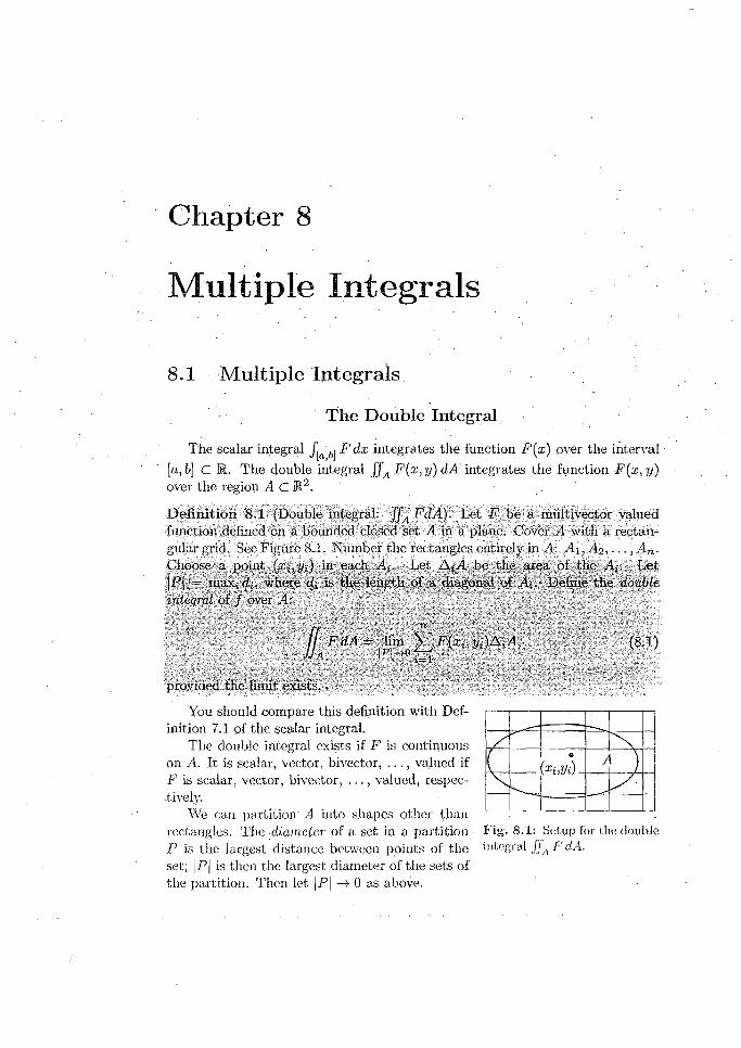
Chapter 8

M ultiple Integrals

8.1 M u ltip le In teg ra ls

T he D ou b le Integral

The scalar integral j a^ F dx integrates the function F(x) over the interval ■

[a, b] C R. The double integral f f A F(x , y) dA integrates the function F (x ,y ) over the region A C R2. . '

D efin ition 8.1 (Double integral: fJA FdA). Let. F be a multivector valued function defined on a bounded dosed set A in a plane. Cover A with a rectangular grid. See Figure 8.1. Number the rectangles entirely .in tI: Aii'A?-,. ■ ■ ,A n .I'lions*- puini (./',.//,) in each .-I;. I.i-i A //l lie t.h<' urea of llie A t. Let WJj ■ m;i>:,(/;. w h ered. is tin-, length of a diagonal of A t. Define the doubh initt/nd of f over A:

/ / F d A = lim F(:it. Vi) A 7A,.//.! i' i rt'f-T '

provided (.In- limit, i-xis!:-.

You should compare this definition with Definition 7.1 of the scalar integral.

The double integral exists if F is continuous on A. It is scalar, vector, bivector, . . . , valued if F is scalar, vector, bivector, . . . , valued, respectively.

We can partition' A into shapes other than rectangles. The diameter of a set in a partition ■ Fig. 8.1: Setup for the double P is the largest distance between points of the integral fJA FdA. set; |P | is then the largest diameter of the sets of the partition. Then let |P | —> 0 as above.

1 1 0 C h a p t e r 8: M u l t i p l e In t e g r a l s

■ For scalar valued / , tlie double integral has many interpretations. Among them: , •

• If / = 1, then f f 4 f d A is the area of A. For then the sum in Eq. (8.1) is approximately the area of A.

• If f ( x , y ) = p(x,y), the mass density over A in, say, grams/cm2, then JJA f d A is the mass of A , in grams. For then the sum in Eq. (8.1) is approximately the mass of A.

•• If / > 0, then f f A f d A is the volume of the solid V above A and under the surface z = f ( x , y ) . For then the sum in Eq- (8;1) is approximately the, volume of V.

There are many other.notations for the double integral: f f A Fdxdy, . f f , F d 2x, f f A F \d 2x.\. Sometimes F is written on the right: JJA dxdyF ,

[]A d2x F , [fA | d 2 x | F, especially in physics texts.

T h e o re m 8.2 (Double integral properties). If the integrai(s) on the right exist, then so does the integral on the left, and equality holds.a. f f A cF dA = c f f A F dA. . . “

b. JfA (F + G ) d A = JfA F d A + .JfA G dA. ■

JLtUA, F d A = fJAl F d A + f f Aa F d A .(Here A i a n d -Ai do not overlap except possibly for boundary points.)

The proof is similar to that of Theorem 7.6 and is omitted.

T h e o re m 8.3 (Integral mean value theorem). Let A be a closed, bounded, and connected set in B.2 with area \A\. Let / be scalar valued and continuous in A. Then there Ls a point (xo-j/o) £ A so that

f f r o , yo) = j j J dA. . (8.2)

Proof. Since / is continuous on the closed and bounded set A, it takes on minimum and maximum values on A: f ( x , n,y ,n) < f ( x , y ) < fi- 'M ■ //a? ) (Theorem 6:2). Integrating and dividing by |A| gives

f { x m, ym) < j!^ f ( x , y) dA < f ( x M, yM). -

Since f ( x , y ) is continuous, it takes on every value between f ( x m,y m) and ,I'(x m , y.M) (Theorem 2.12). In particular, there is a point, (a;<), i/o) satisfying Eq (8.2). ■ □

S e c t i o n 8 .1 : M u l t i p l e I n t e g r a l s 1 1 1

Iterated Integrals

Fig. 8.2: JJA F dA =

fy= c (JL a F dx) dy-

Fig. 8.3: f fA F dA =

jL a ( Iy = 3U F d y)fc-

Fig. 8.4: f fA FdA =

■ fy i j f z = r (y )FdX) dy- .

We turn to the question of evaluating double integrals. Sometimes they can be evaluated analytically. The simplest situation is when A. is a rectangle, as in Figure 8.2. If F is'continuous, then it can be shown that

[ ' [ F d A = f. ( f F ( x ,y ) d x J J a J y = c \ J x = a

dy. (8.3)

The right side is an iterated, integral. The parentheses on the right are usually omitted. The iterated integral is the “composition” of two ordinary.scalar integrals. The “inner” integral f x=aF (x ,y ) dx is evaluated first, holding y fixed, a constant. (We might call this “partial integration” , in analogy with partial

differentiation.) The result is a function of y. The “outer” integral f^ _ c(---)dy integrates this function to a scalar.

Here is an example. Let f ( x , y) — x i r on a unit square ,4 with corners (0,0), (1,0), (1,1), and (0,1). Then

f [ x y 2 dA =J J A J y = 0fJ y = i

i f ' 1

1

x=0

2

xy dx j dy

l

f 1 2/ T yJ y = 0 ^

dyx=0

a . 1 y3 y * / = 2 T

0

The integrand \ y on the right side of Step (3) is the function of y referred to above.

E xerc ise 8.1. I often find it frustrating to evaluate an iterated integral, as it is easy to make a mistake, especially in the more complicated situations below. Evaluate again the iterated integral above using SymPy.

Please be clear about the difference between the double integral on the left side of Eq. (8.3), defined in Definition 8.1, and the iterated integral on the right side used to compute it.

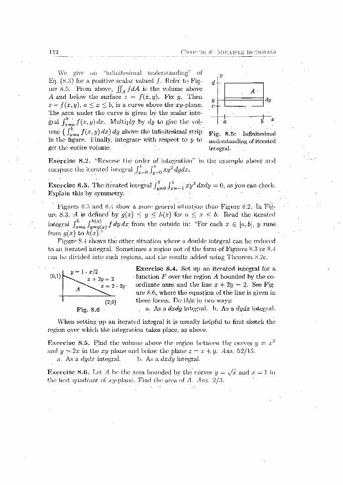
112 C h a p t e r 8: M u l t i p l e I n t e g r a l s

We give an “infinitesimal understanding” of Eq. (8.3) for a positive scalar valued / . Refer to Figure 8.5. From above, fJA f d A is the volume above A and below the surface z = f ( x ,y ) . Fix y. Then

■z = f ( x , y ) , a < x < b, is a curve above the xy-plane. The area under the curve is given by the scalar inte

gral fz—a f ( x , y ) dx. Multiply by dy to give the volr

ume ( f ( x , y) dx) dy above the infinitesimal strip in the figure. Finally, integrate with respect to y to get the entire volume.

A-dy

F ig . 8 .5 : Infinitesimal understanding o f iterated integral.

E xercise 8.2. “R.everse the order of integration” in the example above and compute the iterated integral j j _ 0 f*_0 x y 2 dydx.

E xercise 8.3. The iterated integral' f*_0 f ^ = 1 x y 2 dxdy = 0, as you can check. Explain this by symmetry.

Figures 8.3 and 8.4 show a more general situation than Figure 8.2. In Figure 8.3, A is defined by g(x) < y < h(x) '{or a < x < b. Read the iterated

integral f ^ =a .j f d y d x from the outside in: “For each x G [a, b], y runs

from g(x) to h(x).nFigure 8,4 shows the other situation where a double integral can be reduced

to an iterated integral. Sometimes a region not of the form of Figures 8.3 'or 8.4 can be divided into such regions, and the results added using Theorem 8.2c.

E x erc ise 8.4. Set up an iterated integral for a function F over the region A bounded by the coordinate axes and the line x -j- 2y = 2. See Figure 8.6, where the equation of the line is given in three forms. Do this in two ways:

Fig. 8.6 • a. As a dxdy integral, b. As a dydx integral.

When setting np an iterated integral it is usually helpful to first sketch the region over which the integration takes place, as above.

E xerc ise 8.5. Find the volume above the region between the curves y = x 1 and y =-2x in the xj/-plane and below the plane z = x -\- y. Ans. 52/15.

a. As a dydx integral. b. As a dxdy integral.

E x erc ise 8.6. Let A be the area bounded by the curves y = \fx, and x = 1 in the first quadrant of .i.-y-plaiie. Find the area of A. Ans. 2/3.

S e c t i o n 8 .1 : M u l t i p l e I n t e g r a l s 1 1 3

T he Triple In teg ra l

The definition of the triple integral f f f v Fd,V over a solid V in Ra is analogous to Definition 8.1 of the double integral f f A F d A over an area A in IK2. Interpretations include the volume Jffv d V and the inass fJ'fv p d V of V.

A triple integral can sometimes be computed as an iterated integral. This is similar to the reduction of a double integral to an iterated integral. However, the situation is more complicated in three dimensions: (i) three dimensional regions are much harder to visualize than two dimensional regions, and (ii) there are 3 x 2 = 6 possible orderings for an iterated triple integral instead of the two for an iterated double integral.

As an example, we calculate the volume of the portion of the unit ball x 2 + y 2 + z 2 < 1 in the first octant: x , y , z > 0. Read the iterated integral on the right side of Step (1). below from the outside in: “For each x e [0,1], y runs from 0 to s / \ — x 2, and for each such, a; and y, z runs from 0 to ^ /I — x 2 — y2 ” . Then (x, y, z) varies over the first octant portion of the ball. A sketch might help to picture this. ' ■

rV 1 -X *

d V = / / d z d y d xx= 0 J y ^ O J 'z=0

<"/T-

/x=0 Jy=0\ / l — x 2 — y 2 dy dx (8-4)

y/ 1 — t*2J | [ y V 1 ~ x 2 ~ V2 + (! - x 2) a rc s in ^

(1 - x 2) dx =

I x= 0

i r .......4 J „ o ' 6

dx y=o

The steps of Eq. .(8.4) can be seen “by eye” , except Step (3), which can be checked (laboriously) by differentiation. (Do not bother.)

This iterated integral is complicated. SymPy is no help: it chokes on the iterated integral. Problem 8.2.2b shows th a t spherical coordinates are, unsurprisingly, better suited to the problem, yielding an easily computed iterated integral.

Here is a technique for evaluating some triple integrals. Let V be the region in R3 above and/ or below the region A in the iy-plane and between the surfaces .z = ffi(x.y) and z = g2(x ,y) , g i(x ,y ) < g2(x ,y) . Then

f f l f ( x , y , z ) d Y = [ [ [ JAJ"V) f ( x , y , z ) d z d A .JJJ V J J A J z~gx (i,y)

Think of f ( x , y, z) d zd A as the infinitesimal part of f f f v f dV above/below dA. First evaluate the inner integral, then the double integral.

E xercise 8.7. Let A be the area bounded by the curves y — %/x and x — 1 in the first quadrant of j;y-plane. Let V be the solid above A and below the plane z = 1 + x + y. Compute [fjv 6xydV . Cf. Exercise 8.6. Ans. 65/28.

1 1 4 C h a p t e r 8: M u l t i p l e In t e g r a l s

Hero is another technique for iterating some triple integrals. Suppose thatV lies between the z = a and z = b planes. Slice V a t 2 , giving the region A z .

Think of JJA f ( x , y ; z ) dAz dz as an infinitesimal piece of f f f v f dV at height z.

plane x / a + y/b + z /c = 1, a, b, c > 0. I used SymPy. Ans. abc/6.

8.1.2. The salinity of the oceans varies from place to place. Let s(P) be the .salinity at point P, in grams of salt per cubic centimeter. Express the total amount of salt in all the oceans in grams as an integral.

8.1.3. Evaluate ff jv (x2 + y~)dV, where V is the tetrahedron bounded by the planes z = x + y, x = 0, y = 0 and z — I. Ans. 1/30.

8.1.4. Evaluate the iterated integral ]y=0 J.,2=0 x 3y2 cos(x2ys) dxdy to 5 decimal places. Use SymPy.

8.1.5. Evaluate f* e~y*dydx by hand. You will find th a t you cannot do this without switching the order of integration. Ans. |{1 — e_ l ).

8.1.6. This problem is a. continuation of Problem 7.3.4. It culminates in Eq. (9.11). Recall that F = F (x (u ,v )) . Give reasons for the steps:

Then■6

Double and triple integrals can be generalized to n-dimensional regions in Rn. The general term is multiple integral. Hence the title of this chapter.

Problem s 8.1

8.1.1. Compute as iterated integrals.a. The area of the triangle bounded by the coordinate axes and the line

x /a + y/b = 1, a, b > 0.b. The volume of the tetrahedron bounded by the coordinate planes and the

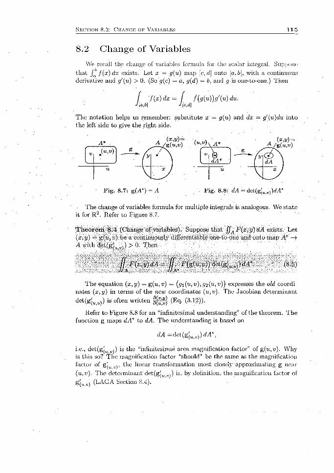
S e c t i o n 8 .2 : C h a n g e o f Va r i a b l e s 1 1 5

8.2 C h an g e of V ariables

We recall the change of variables formula for the scalar integral. Suppose

that Ja f ( x ) d x exists. Let x = g(u) map [c,d] onto [a,b], with a continuous derivative and g'(u) > 0. (So g(c) — a, g(d) — b, and g is one-to-one.) Then

[ / (x) dx = f f(g(u))g'(u)du.- J (a,6] J [cyd\

The notation helps us remember: substitute x = g(u) and dx = g'(u)du into the left side to give the right side.

F ig . 8 .8 : dA = det(g'(UiV))dA*

■ The cha.nge of variables formula for multiple integrals is analogous. We sta te it for R 2. Refer to Figure 8.7.

T h e o re m 8 .4 (Change of variables). Suppose that f f A F (x ,y ) dA exists. Let (x .y) — g(%v):.;be a continuously differentiable one-to-one and onto map # —> A with det(g ,ti ,,-) > 0. Then

F (x , y ) d A = j j ^ F(g(w, vj) det(g'(UiU)) dA*. (8.5)

The equation (x , y ) = g (u,v) = (g i(u ,v) ,g2(u,v)) expresses the old coordinates (x, y) in terms of the new coordinates (u,v). The Jacobian determinant

d e t(g(u,«)) is often written (Eq. (3.12)).

Refer to Figure 8.8 for an “infinitesimal understanding” of the theorem. The function g maps dA* to dA. The understanding is based on

dA = d e t(g (U)j;)) dA*,

i.e., de t(g |u ^ ) is the “infinitesimal area magnification factor” of g (u,v). Why is this, so? The magnification factor “should” be the same as the magnification factor of gju vy the linear transformation most closely approximating g near

(u,v). The determinant det(gju 7 ) is, by definition, the magnification factor of

£(u,v) (LAGA Section 8.4).

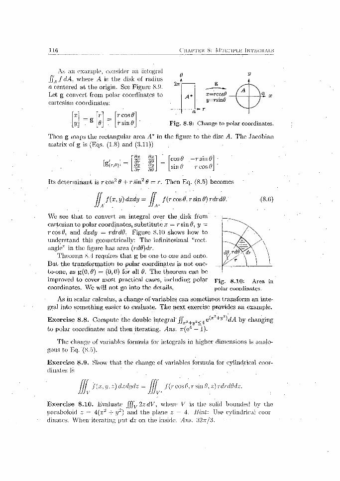
116 C h a p t e r 8: M u l t i p l e In t e g r a l s

As an example, consider an integral JjAf d A , where A is the disk of radius a centered at the origin. See Figure 8.9. Let g convert from polar coordinates to cartesian coordinates:

2tt

X r rcosd

y-.= g 8 rs in #

A* x=rcosO «/=rsin 8

Fig. 8.9: Change to polar coordinates.

Then g maps the rectangular area A* in the figure to the disc A. The Jacobian matrix of g is (Eqs. (1.8) and (3.11))

dx

dt , dr

dx86ay80

cos 8 —r sin 8 sin 8 r cos 8

■(8 .6 )

[g ( r ,0 ) JL 3t

Its determinant is r cos2 8 + r sin2 8 = r. Then Eq. (8.5) becomes

J J f ( x , y ) dxdy = JJa f ( r cos-6, r sin 8) rdrdd.

We see that to convert an integral over the . disk from cartesian to polar coordinates,, substitute x = r sin 8, y = rcosd, and dxdy — rdrdd. Figure 8.10 shows how to understand this geometrically: The infinitesimal “rectangle” in the figure has area (rdd)dr.

Theorem 8,4 requires that g be one-to-one and onto.But the transformation to polar coordinates is not one- to-one, as g (0 .8) = (0,0) for all 9. The theorem can be improved to cover most practical cases, including polar p |g_ g.xo: Area in

polar coordinates.coordinates. We will not go into the details.

As in scalar calculus, a change of variables can sometimes transform an integral into something easier to evaluate. The next exercise provides an example.

E x erc ise 8 .8. Compute the double integral Jfx2+y-2<4 e(x2+y2)dA by changing

to polar coordinates and then iterating. Ans. 7r(e4 — 1).

The change of variables formula for integrals in higher dimensions is analogous to Eq. "(8.5).

E x erc ise 8 .9. Show th a t the change of' variables formula for cylindrical coordinates is

/(./■. y, z) dxdydz ■ / (r cos 8, r sin 0, z) rdrdOdz

E x erc ise 8.10. Evaluate f f f v 2zdV , where V is the solid bounded by the paraboloid z = 4(x2 + ?/2) and the plane z = 4. Hint: Use cylindrical coordinates. When iterating put d z on the inside. An,s. 327r/3.

S e c t i o n 8 .2 : C h a n g e o p V a r i a b l e s 1 1 7

P rob lem s 8.2

8.2.1. Compute the volume inside the paraboloid z = x 2 + y 2, 0 < z < 1. Ans. t t / 2 .

8.2.2. a. Show that the change of variables formula for spherical coordinates is

f ( x , y , z) dxdydz

f(psin(j)Cos8,psm(j)sm8,pcos (j>) p2sin (j> dp d(j>dO.

1

-Iff,Recall Problem 3.3.3.

b. Compute the volume of a ball of radius p0 using an iterated • integral and spherical coordinates. Compare the difficulty of vour calculation to that of Eq. (8.4).

8 .2 .3. Find the volume of the ellipsoid x 2/ a 2 + b2/c2 + z 2)<? < 1. Hint: Substitute u = ax, v = by,w = cz. Ans. 4irabc/3.

8.2.4. A solid made of a metal alloy lies within the cylinder x 2 + y 2 = 1, below the plane z = 4, and above the paraboloid z = 1 — x 2 —y 2. The cost, in $/cm 3, of the metal is twice the distance to 'th e z-axis. Find the cost of the solid. Use the coordinate system best suited to this problem. Ans. 24ti/5.

8.2.5. Let .4 = . Then x A vl maps the unit ball in R3 to some1 4 7 0 2 90 0 3

solid. Find the volume of the solid. This can be done without paper and pencil.Ans. 8tt.

8.2.6. Find the volume inside the cylinder x 2 + (y — l ) 2 = 1 above the xy-plane and below the paraboloid 4z = x 2 + y 2. Hint: Sketch the circle x2+ (y — l ) 2 = 1. ,4ns. 37t/8.

8 .2.7. Evaluate the integral f f A ev+* dA, where A is the region bounded by the lines x = 0, y = 0, x + y = 1. Hint: Substitute u = y+ x and v = y —x. Translate the equations of the boundary lines from xy-coordinates to uv-coordiuates. .4ns. ( e - e - 1) / ^

In this problem it is easy to solve for x and y in terms of u and v to compute the Jacobian determinant. In other cases it is hard to impossible. Then we can use the Inverse Function Theorem 3.12 and LAGA Theorem 8.24.

8.2.8 . Suppose that A is a disk of radius.a centered at the origin and th a t / is symmetric around the origin, i.e., it is a function only of r. Show th a t

I f A f ( r ) dA = 2lr lo r/('r) dr■

Chapter 9

Integrals over Surfaces

9.1 T h e Surface In teg ra l

This chapter introduces two kinds of. integrals for fields on surfaces. The first, simply called the surface integral, is the topic of this section. We denote it JJ-S f dS, where dS is a scalar. The surface integral is to surfaces what the' path integral is to curves. See Figure 9.1.

The second, the flux integral, is the topic of the next section. We denote it JJS f dS, where dS is a bivector. The flux integral is to surfaces what the line integral is to curves. Put another way, the flux integral is to the surface integral what the line integral is to the path integral.

We define the surface integral by reducing it to a double integral.

D efin itio n 9.1 (Surface inu^ral: JJS F dS). l.ri. F be a field on a surface S C E ” . Par;jmd erize 8: x(u.,v): A C Ti2 ■ » S. Then the surface integral of F over iS' is defined by

J j F d S = U ' F (x (u ,u )) |x„(w, v) A dA. (9.1)

This is a generalization of Definition 7.5 of the path integral:

. [ F d s = f F(x(t))\x'(t)\d,t.J C -J [a‘,6]

Curve C Surface S

. Path Surface,

I c F d s I I s F d Sds a length dS an area

Line Flux

S c F d s I I s F d S

ds = t ds, dS = B d S ,a vector a bivector

F ig . 9 .1: Integrals over m anifolds.

1 2 0 C h a p t e r 9: I n t e g r a l s o v e r S u r f a c e s

Wo give an “infinitesimal understanding” of Eq. (9.1). On the left side, dS is the area of an infinitesimal piece of-S'. Multiply dS by the value of F at some point in the piece: F d S . Sum (integrate) to form the surface integral j f s F d S .

For the right side use

x(u,vf~^P> d S = A I dA’ (9-2)

x iu+dtis j) / i.e ., |x„(tz, v) A x v(u, w)| is the “in- (u+ u,v) finitesimal magnification factor” of

Fig. 9.2: Ihe surface integral. x 'J'q see this, refer to Figure 9.2:

d S = | (x(i/, + du, v) — x(u, v )) A (x(u, v + dv) — x ( m , ■?;)) |

= \xu(u,v)du f \ x v(u,v)dv\

= Jx?1(u,-u) A x„(w, »;)| dA,

Multiply by F and integrate to form Eq. (9.1). .

In R3, (xu A x„ )* = x u x Xj, (Eq. (4.1.1)), so |x „ A x „ | = |x „ x .x t,|. Thus we may write Eq. (9.1) as

. JJ' F d S = JJ F (x (u ,v ) ) |xu(ji,«) x x v(u ,v)\dA: (9.3)

E x erc ise 9 .1. Represent a surface S by z = f ( x , y), (x ,y) € A. Show that

J J F d S = JJ^ F ( x , y, f { x , y)) 1 -1- ( f j x , y))2 + ( f y (x, y ) )2 dA. (9.4)

Problem s 9.1

9.1.1. Consider the surface z = 2(x2 + y2)3 above the region x 2 + y 2 < 4 in thexity-plane. Suppose the density of the surface above (x ,y) is (x2 + y2 + z2)^, in suitable units. Find the mass of the surface. Ans, 80tt/3.

9.1.2. Recall the definition of Jacobian determinants like "(Eq. (3.12)).

Show that |x u(u,t>) A x v(u ,u)| in Eq. (9.1) is given by

i i w , ^ 2 ( d ( y , z ) \ 2 t f d ( z , x ) \ 2 ( d (x ,y)|x„(w, v) A x v(u, v)\~ = -w .— r + w,-----f +

J ) (u ,v ) J \ d ( u , v ) J ' \ d ( u , v )

Start with Eq. (1.4).

9.1.3. Show th a t if the surface integral(s) on the right exist, then so does the integral on the left, and equality holds.

a. f l s cF d S = c Jjs F dS.

1) . j f s (F + G) d S - [f., F d S + Jjs G dS.

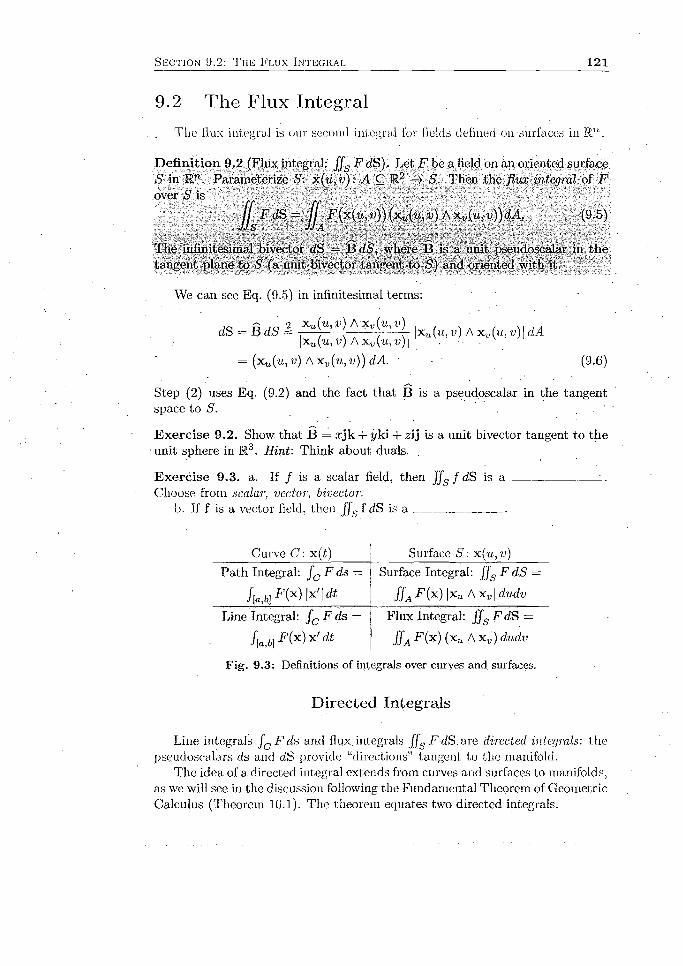
S e c t i o n 9 .2 : T h e F l u x I n t e g r a l 1 2 1

9.2 T h e F lux In teg ra l

The llux .integral is our second integral for fields defined on -surfaces in Ru .

D efin itio n 9.2 (Flux integral: Jjs F d S ) . Let F be a field on an oriented surface S in Rn . Parameterize S: x ( u ,v ) : A C K2 -» S. Then the flux integral of F .over S' is

tangent plane to S (a unit bivector tangent to S) and oriented with it.

We can see Eq. (9.5) in infinitesimal terms:

Step (2) uses Eq. (9.2) and the fact that B is a pseudoscalar in the tangent space to S'.

E x e rc ise 9.2. Show that B = rrjk + t/ki + zij is a unit bivector tangent to the unit sphere in R3. Hint: Think about duals. .

E x e rc ise 9.3. a. If / is a scalar field, then JJS f dS is a _____________ :.Choose from scalar, vector, bivector.

b. If f is a vector field, then f js f dS is a ______________

Line integrals f c F d s and flux, integrals JJS F dS.are directed integrals: the pseudoscalars ds and dS provide “directions” tangent to the manifold.

The idea of a directed integral extends from curves and surfaces to manifolds, as we will see in the discussion following the Fundamental Theorem of Geometric Calculus (Theorem 10.1). The theorem equates two directed integrals.

(9.5)

The infinitesimal bivector dS — B dS, where B is a unit pseudoscalar in the

dS = B dS =g d s ^ X u ( u , v ) A x v(u,y)

|xu(it, v) Ax„(«, u)|

(xu(u,v) A x v(u,v)) dA. -

|x u (u, v) A x v{u, v)\dA

(9.6)

Curve C : x(t) Surface S : x(u, v)

Path Integral: f c F d s = Surface Integral: f f s F d S =

/(a,6] F (x) lx' Idt ffA F (x) lx“ A I dudv

Line Integral: f c F ds = Flux Integral: f f s F dS =

f[a,b] F ( x ) x ' cit f f A F (x ) (xu A Xv) dudv

Fig. 9.3: Definitions of integrals over curves and surfaces.

D irected Integrals

1 2 2 C h a p t e r . 9: In t e g r a l s o v e r S u r f a c e s

T h e Vector d a

The bivector dS prevents vector calculus from forming the flux integral J jg F d S , Instead, in R3 it uses an infinitesimal vector orthogonal to dS:

d a = (dS)* = (B dS)* = B* dS = n d S , (9,7)

where n is a unit vector orthogonal to S .1 Think of dcr as an infinitesimal piece of the surface dS with the tail of n attached to it. We can then form JJS F dcr, also called a flux integral. ' ’ ■

T h eo rem 9.3 (Compute dcr integral). Lot F bo a riiultivector field on a surface S C ft3. Parameterize S. with x(m, ?/) : ~'A:Q R2 —>■ S. Tlieri ,

J J Fdcr — JJ F (x) (x u x x„)<L4. (9.8)

Proof. We give an infinitesimal proof using Eq. (9.6) in Step (2):

dcr = (dS)* = ((xu A.x„) dA)* = (xu x x v)dA. □

Vector calculus can form f f s f dcr for a scalar field / but not ffs f dcr for a vector field f. However, it does form the very useful scalar valued integrals

j j f ’ dcr and j j (V x f) • dcr.

We will see those integrals in important vector calculus theorems in Sections 10.2 and 10.3.

E xerc ise 9.4. Let f (x ,y , z) = a ii+ < i2j +<23k be a constant vector field. Let S be the unit sphere x 2 + y 2 + z 2 = 1. Determine f f s f - dcr without a calculation.

The scalar part of Theorem 9.3 for a vector field gives this corollary.

C o ro lla ry 9.4. Let f be a vector field on a surface S C Rn. Parameterize! S widi x ( i/ ,r ) : .4 C i?-" > Then

JJ f -dcr= JJ f (x) - (x^ X x v) dA. . . . . (9.9)

E xercise 9.5. Let 5 be the surface z = x 2 + y 2, 0 < z < 9. Compute the integral JJS. f • da, where f (x , y) — — 2:j;x — 2yj + k. Ans. 171 tt.

1 In \voctor ca lcu lus te x ts o u r dcr is o ften d en o ted dS . O u r d,S, a bivcclor, has no c o u n te rp a r t iii vec to r calculus.

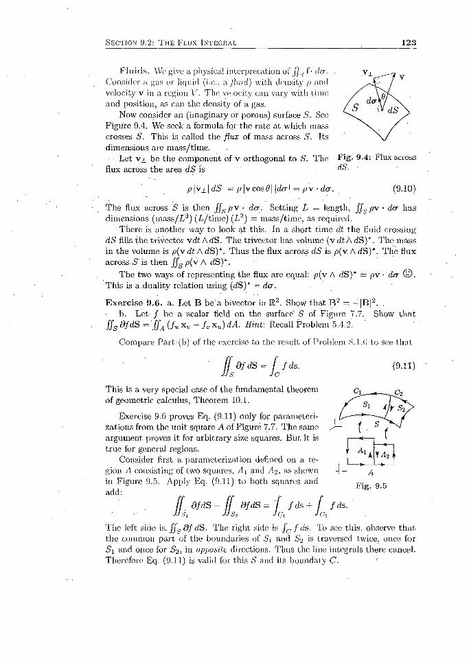
S e c t i o n 9 .2 : T h e F l u x In t e g r a l 1 2 3

Flu ids. We give a physical interpretation of JJS. f • da. Consider a gas or liquid (i.e., a fluid) with density p and velocity v in a region V. The velocity can vary with time and position, as can the density of a gas.

Now consider an (imaginary or porous) surface S. See Figure 9.4, We seek a formula for the rate at which mass crosses S. This is called the flux of mass across S. Its dimensions are mass/time.

Let vj^ be the component of v orthogonal to S. The flux across the area dS is

F ig . 9 .4 : Flux across dS. ■

/o|vj_|c(5 — p \v cos 9\\dcr\ = p v • da. (9.10)

The flux across S is then f f s p v • dcr. Setting L = length, f f s pv ■ da has dimensions (m ass/L3) (L/time) (L2) = mass/time, as required.

■ There is another way to look at this. In a short time dt the fluid crossing dS fills the trivector vdt AdS. The trivector has volume (v dt A dS)*. The mass in the volume is p(v dt A dS)*. Thus the flux across dS is p(v. A dS)*. The flux across .S is then f f s p(v A dS)*.

The two ways of representing the flux are equal: p(v A dS)* = pv - da © . This is a.duality relation using (dS)* = da.

E x erc ise 5.6. a. Let B be'a bivector in IE2. Show that B 2 = — |B |2.b- Let / be a scalar field on the surface S of Figure 7.7. Show th a t

f f g d fd S — ffA ( f u x.v — f v x u)dA. Hint: Recall Problem 5.4.2.

Compare Part (b) of the exercise to the result of Problem to see that,

(9.11)f l^ fd S = J jd s .This is a very special case of the fundamental theorem of geometric calculus, Theorem 10.1.

Exercise 9.6 proves Eq. (9.11) only for parameterizations from the unit square A of Figure 7.7. The same argument proves it for arbitrary size squares. But, it is true for general regions.

Consider first a parameterization defined on a region A consisting of two squares, A i and A%, as shown in Figure 9.5. Apply Eq. (9.11) to both squares and add:

d f d s + [ [ d fdS = f f d s + f 'Si JJ S2 J c J J c2

The left side is. [Js d fd S . The right side is fc f ds. To see this, observe that the common part of the boundaries of Si and S2 is traversed twice, once for S i and once for S-2, in opposite directions. Thus the line integrals there cancel. Therefore Eq. (9.11) is valid for this S and its boundary C.

f d s ..

124 C h a p t e r 9: In t e g r a l s o v b r S u r f a c e s

Given an arbitrary parameterization A S, approximate A with squares inside it. Then Eq. (9.11) holds for their union. Now take the limit as the squares come closer and closer to filling A. I t is plausible that this gives Eq. (9.1.1) for A.- .

P roblem s 9.2

9.2.1. Represent a surface S by z = g(x ,y) , (x , y) 6 A. Let F be a multivector field on S. Show that

Fdcr = J J F (x , y;g(x, y)) ( - g j x , y )i - gy(x, y)j + k) dA.

Recall Exercise 9.1,There is a. useful corollary to this formula for a vector field f = / i i + / 2J’+ / 3k:

■ J J f - d a = J J ( - f 1gx - f 2gy + h ) ( iA .

9.2.2. Let B = (x 2 -\-y2 + z2)~3/,2(ayk + y k \ -M ij). Compute JJs B -d S , where S is the unit sphere. Hint: You might find it helpful to.compute (xi + y] + z k )* and remember its geometric meaning. Ans. —4ti\

9.2.3. The right side of Eq. (9.1.1) is a vector. Thus the left side is a vector. However, on the left side 9 fd S is “(vector) (bivector)” which in general is “scalar + trivector” (LAGA Theorem 6.5). Explain directly why OfdS lias no trivector part.

Part IV

The Fundamental Theorem of Calculus

Chapter 10

The Fundamental Theorem of Calculus

The Fundamental Theorem of (Geometric) Calculus is the capstone of this book. It is a far reaching generalization of the Fundamental Theorem of (Scalar)

Calculus, f F ' dx = F(b) — F(a), and of standard theorems of vector calculus we will see in Sections. 10.2 and 10.3.

10.1 T h e F u n d am en ta l T h e o re m of C alcu lus

The fundamental theorem is built from the vector derivative (Section 5.5) and the directed integral (Page 121). Its statement is so simple and so general that we give it right off. Then we will discuss the meaning of its several parts. A proof is beyond the scope of this book.1

Until now, we have written the infinitesimal in an integral to the right of the function to be integrated. This is in accord with nearly universal practice in vector calculus texts. But the simplest expression of the fundamental theorem has the infinitesimal to the left.

T h eo rem 10.1 (Fundamental Theorem of (Geometric) Calculus). Let M be an oriented and bounded m-dimensional manifold with boundary d M .a

Let F be a continuous multivector field on M with a continuous vector derivative OF on M — 8M . Then

I dmx d F = ( f> dm_1x F . (10.1) JM JdM

“Yea, I know, yet another use of the symbol d. Sorry, but tliese: are standard notations.

The m-dimensional manifold M is in some Rn. But which Rn is irrelevant for the theorem, except that rn < n (of course).

*G. Sobczyk an d O. Sanchez, Fundamental Theorem o f Calculus, A dv. A ppl. Clifford Algebras 21 221-231 (2011). Also available a t h t t p : / / a r x i v . o r g / a b s / 0 8 0 9 . 4 5 2 6 .

http://arxiv.org/abs/0809.4526

128 C h a p t e r 10: T h e F u n d a m e n t a l T h e o r e m o p C a l c u l u s

D iscussion o f th e F u n d a m e n ta l T h e o re m

M . In M3 the possibilities for the manifold M are solids V (m = 3), surfaces S (m = 2), and curves C (rn = 1). See Figures 10.1-10.3..

+1 .

n

F ig . 10 .1: A solid. F ig . 10 .2: A surface. F ig . 10 .3 : A curve.

3 M . We cannot give the technical definition of the boundary d M of M . Intuitively, think of the “edge” or “border” of Af. See the figures. The boundary d M is a manifold of dimension one less than M . The boundary d V of a solidV is. its surface. In Figure 10.1 the boundary is -the side, top, and bottom of the cylinder. The boundary of a solid can have more than one piece, e.g., the solid between concentric spheres. The boundary d S of a surface S is a curve, or curves as in Figure 10.4. The boundary dC of a curve C is its endpoints! See Figure 10.3,

d mx. We first describe dmx, the infinitesimal of multiple integrals. The “m” is the dimension of the manifold over which the integration takes place. Think of dmx as the infinitesimal m-volume of an infinitesimal piece of M . The symbol dmx provides a uniform notation for path integrals from Definition 7.5 (ds -* d 1x), multiple integrals from Section 8.1 (dA -»• d2x and dV -» d3x), surface integrals from Definition 9.1 (dS —> d?x), and their generalizations to higher dimensions. Only one integral sign is used. (Fifty integral signs for an integral over a 50-dimensional manifold is not practical.) For example, F dAx is the integral of the field F over the 4-dimensional manifold M C Rn, n > 4.

The directed integrals in Eq. (lO.'l) use infinitesimals of the form dmx. Define dmx = l rndmx, where ITO = Im(x) is the unit pseudoscalar of the tangent space to M a t x. Thus dmx. is an infinitesimal pseudoscalar in the tangent space, an infinitesimal m-vector with infinitesimal m-volume dmx. It thus has a “direction”. The symbol dmx provides a uniform notation for line integrals from Definition 7.S (ds = i d s —> d1x ), flux integrals from Definition 0.2 (dS =

TBdS —>• d2x), and their generalizations to higher dimensions. For example, fM F d4x is the directed integral of the field F over the 4-dimensional manifold M C IRn, n > 4, '

From d mx = Imdmx, we see that dmx can be manipulated algebraically as an m-vector. For example. v d 2x = —d ? x v for vectors v in R2.

Neither dmx and d F nor d m~ lx and F in Eq. (10.1) commute in general, as they are multivectors. The infinitesimal scalar drnx commutes with everything.

S e c t i o n 10.1 : T he F u n d a m e n t a l T h e o r e m o f C a l c u l u s 1 2 9

D irec ted In teg ra l. Understand the directed integral dmx F as an integral over the m-diinen.sioiial manifold M. Define the directed integral as a multiple integral 011 E m. Definitions 7.8 and 9.2 lead the way. First parameterize M with x (u 1 ,U2, ■ ■. ,u m): A c —> M C M n . Then define

[ dmx F = f (xUl J M J A

Ax„ • Xu J d A F { x ) . , (10.2 )

O rie n ta tio n . The orientations of M and c)M must be chosen consistently in the fundamental theorem, as a change of orientation changes the sign of directed integrals. Here is the rule, followed by examples. Let n be the unit outward (boundary) normal to M . See Figures 10.1-10.3. Then the pseudoscalar I m orienting M and the pseudoscalar Im_i orienting c)M must be chosen so that Im = Im_i_n. The negatives of both choices are. also acceptable, for then (—Im) = (—Im_i)n.- We describe the standard choices for solids, surfaces, and curves.

Figure 10.1. The outward boundary normal n to V is shown. (In this case it is also the unit normal n to dV.) We choose I 2 = e ie 2 and thus I 3 = e ^ n .

Figure 10.2. The outward normal ii to S is shown. (It is different from th e unit normal n to the surface.) We choose I i = e j and thus I 2 = e jf i .2

Figure 10.3. The outward normals n to C at its two 0-dimensional boundary points are shown. Their orientation Io is given by 0-dimensional unit pseudoscalars, i.e., unit scalars, ± 1 . At the terminal end we choose Io = +1 and. thus I j = (+ l)n , as shown.

H oles in M . The fundamental theorem admits manifolds with holes. The boundaries facing the holes are part of dM , and oriented with the same rule, Im_ in - I m, as above. Figure 10.4 shows an example.

Fig. 10 .4: A hole in S. Fig- 10 .5: S = S 1 U 52-

Figure 10.5 shows that allow’ing the hole in Figure 10.4 is consistent with a “holeless” fundamental theorem. The dashed lines in Figure 10.5 divide S into two surfaces without holes, S\ and i>2 -. Apply the “holeless” fundamental theorem to each and add:

J dmx ( ) f ■ dmx OFr

f ' ./as,drn~i x F + d) d 'n_1x F.

d S 2 '

2T h e re la t iv e orient,a(,ion of S and 9 S in F ig u re 10.2 is requ ired for u n ifo rm ity in th e fu n d a m e n ta l th e o re m across g rades an d d im ensions . T h e o p p o s i te o r ie n ta t io n of d S is s t a n d a rd in vector calcu lus . T h e clash is u n fo r tu n a te . See C oro lla ry 10.5.

13 0 OllAI’TKIl 10: TH E FUNDAMENTAL THEOREM 01' CALCULUS

The left side is J s, d '" x d F . Oil the right side, the line integrals over the dashed line parts of the boundaries of Si and S2 are traversed twice, in opposite directions, as shown. Because the line integrals are directed, they cancel, leaving

i s r ' l x F ' ■ •An S with several holes can be handled with more complicated “surgeries” .

E xercise 10.1. a. Show that <ftgM = 0 for every bounded manifold Af.b. The boundary d M in Part (a) could be a sphere, the boundary of a ball

in R3. Explain in geometric terms why Part (a) is expected in this case.

E xercise 10.2. A theorem states that if M is a bounded manifold, then d M is closed? i.e., has no boundary: d(dM ) = 0. Thus we use <faM in Eq. (10.1),

. just as we use <fc for closed curves. .Show th a t dm~ lx d F = 0 for every field F defined on the boundary.

In the next two sections we specialize the fundamental theorem in different ways and then obtain standard theorems of vector calculus in K3 for solids V (m = 3), surfaces S (m = 2), and curves C (m = 1). For simplicity of exposition,I do not mention the continuity required by the fundamental theorem.

Problem s 10.1

10.1.1. Let S be the cylinder x 2 + y 2 = 1, 0 < z < 1, without a top or bottom. The boundary of S consists of two circles, x 2 + y2 = 1 at z = 0 and 2 = 1. Orient S counterclockwise as seen from the outside. Describe the orientation of its boundary required by the fundamental theorem.

10.1.2. Let M be the solid m-dimensional ball of radius r in RTO (|x| < r) and d M be its (m — l)-diinensional surface (jxj ■ r). Let M have “volume” \M\ and d M have “area” \dM\. Hint: Recall Exercise 5.5.

a. Show that m\M\ = r\8M\.b.. Verify the formula of Part (a) for m = 2 and m = 3.

As witli c;!u.se(J cnrvc.s an d .suriVicc.s, (Jii.s is diiicrciil frum (lie c:lcxsed scsls of Definition 2

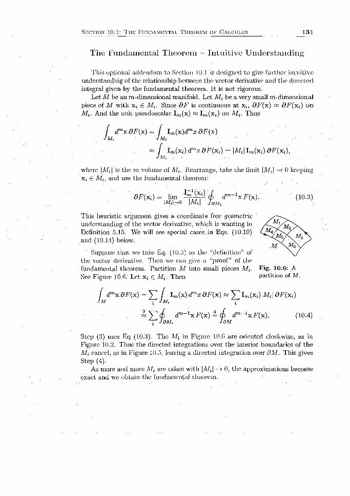
S e c t i o n 10 .1 : T h e F u n d a m e n t a l T h e o r e m o f C a l c u l u s 1 3 1

The Fundam ental Theorem - Intu itive U nderstanding

This optional addendum to Section 10.1 is designed to give further intuitive understanding of the relationship between the vector derivative and the directed integral given by the fundamental theorem. It is not rigorous.

Let M be an m-dimensional manifold. Let M l be a very small m-dimensional piece of M with x» € M i. Since d F is continuous at Xj, d F (x ) « d F (x i ) on Mj. And the unit pseudoscalar I,n(x) « Im (xj) on Mj. Thus

f cF'xdFix.) = ( Im(x)dmx d F ( x ) JMi JMiI Mi JMi

I m(xj) dmx 8F {x i) = |Mj| Im(xj) dF (x i) ,JJMi

where \M{\ is the m-volume of Mi. Rearrange, take the limit \Mi \ —> 0 keeping Xj G Mi, and use the fundamental theorem:

' d F ( x i ) = lim J ™ j y 4 rfm_1x F (x ) . ' (10.3)\M i\->0 I Mi I T dM i ■

This heuristic argument gives a coordinate free geometric understanding of the vector derivative, which is wanting in Definition 5.15. We will see special cases in Eqs. (10.10) arid (10.14) below.

. M \ KSuppose that we take Eq. (10.3) as the “definition” of

the vector derivative. Then we can give a “proof” of the fundamental theorem. Partition M into small pieces Mj. Fig* 10.6: A See Figure 10.6. Let Xj £ Mj. Then partition of M.

Ldmx d F ( x ) = ] T f Im{x)(Tnx d F { x ) « ^ I m(x i)|Afi | 8F {xi)

M

dm- l x F [ x ) = ({) c T - ' x F f x ) . (1Q.4)i J d ' M i J d M

Step (3) uses Eq (10.3). The Mi in Figure 10.6 are oriented clockwise, as in Figure 10.2. Thus the directed integrations over the interior boundaries of the Mi cancel, as in Figure 10.5. leaving a directed integration over dM . This gives Step (4).

As more and more M l are taken with \Mi\ —*■ 0, the approximations become exact and we obtain the fundamental theorem.

1 3 2 C h a p t e r 10: T h k F u n d a m k n t a i , T i i u o r u m o p C a l c u l u s

10.2 T h e D ivergence T h eo rem

This section specializes the fundamental theorem to 7n-dimensional manifolds M in JEm■ The most important case is (3-dimensional) solids in R3, as illustrated by Figure 10.1.

T h e o re m 10.2. Let F be a multivector field on a bounded m-dimensional manifold M in R m with outward normal fi. Tlien0

f V F ( r x = (£ a F d m7'1x. (10.5)JM -Id At

“We write the infinitesimal to the right when we can.

Proof. Since M has the same dimension as W n, 0 = V. Also, I m, the unit pseudoscalar of R,n, is const,ant over M . On dM ,

. d m~1x = I m_i d m~ 1x = I mncfm-1x. . (10.6)

For Step (2), multiply = Im on the right by n.Substitute into, the fundamental theorem and cancel the I m. □

The outward normal n of an m-dimensional manifold M in Rm is orthogonal to dM. So we can substitute it for n in da = n dS (Eq. (9,7)) which defines the flux integral F d a in R3.

If F = f, a vector field, in Eq. (10.5), then both sides of the equation are “(vector)(vector) = scalar + bivector” . Equating separately the scalar and bivector parts gives two corollaries. The scalar part is the divergence theorem.

C o ro lla ry 10.3 (Divergence theorem). Let f be a vector field on a bounded ?7i-dimensional manifold M in Rm. Set. da = f idm'~Lx. Then

f V - f d mx = ( j ) f -da . (10.7)J M J d M

In R3, set M = V and d M = 5 'and write

J j j V - i d Y = J f j ' d a . (10.8)

This also called Gauss’ theorem. It is a widely used theorem of vector calculus. (The symbol denotes an integral over a closed surface, just a,s <pr denotes an integral over a closed curve.)

E x erc ise 10.3. Verify the divergence theorem for the ball of radius p in R3 and f(.r, y, z) = ;ri + y] + z k.

E x erc ise 10.4. Compute </|\.(?yj + x zk ) • d a , where S is the unit sphere in R3. Ans. 47r/3.

S e c t i o n 1 0 .2 : T h e D i v e r g e n c e T h e o r e m 1 3 3

In E'! with F — f, the dual of the bivector part of Eq. (10.5) is

JJJ V x i d V = JJ da x f, (10.9)

a result not often seen in vector calculus texts.Corollary 10.3 substitutes a vector field v into Eq. (10.5). Problem 10.2.2

asks you to substitute a scalar field / and a bivector field B.

T he G eom etry o f th e D ivergence

The discussion to follow is both instructive and not rigorous. It is analogous to the discussion of th e fundamental theorem on Page 131.

Suppose that V - f is continuous .at xo. Let V be a small ball or cube in R 3 centered at xo and with boundary S. Then for some x* G V,

Step (1) is the analog of Theorem 8.3 for volume integrals. Step (2) is the divergence theorem, Eq.(10.8). Now let |V| 0:

(V • f)(xo) = ‘ Umo ±JJs f - d a . . (10.10)

Less precisely, in words:

(V • f)(xo) is the flux o f f per unit volume away from xo.

This heuristic argument gives a coordinate free geometric understanding of the divergence, which is wanting in Definition 5.4.

Some authors “define” the divergence with Eq. (10.10), which is analogous to Eq. (10.3). This has the advantage of giving the divergence a geometric meaning right away. Then the divergence theorem can be “proved” analogously to Eq. (10.4). Representations of the divergence in various coordinate systems,e.g., cartesian (Eq. (5.4)) and cylindrical and spherical (Page 72) then become just that: different mathematical representations of the same geometric object in different coordinate systems.

1 3 4 ( ’ i i A i n m 10: T i | i - : F u n i m m b n t a l . T h k o r e m o k C a l c u l u s

P roblem s 10.2

10.2.1. Evaluate by the divergence .theorem: £ps (x2i + y 2j + z 2k) - da, where S is the surface of the unit cube 0 < :/: < I, 0 < y < I, 0 < z < 1. Use SymPy. Ans. 3.

10.2.2. Let M be a bounded m-dimensional manifold in Rm.a'. Let / be a continuously differentiable scalar field on M . Prove:

f V f d mx = ( j ) f d a .-JM J dM

b. Let B be a continuously differentiable bivector field on M . Prove:

f V A B d n x = < £ dcr A B.J M ■ J d M

10.2.3. Do Problem 10.1.2 in R3 using the divergence theorem..

10.2.4. Define the Lapiacian A == V 2. Since V “is” a vector, A “is” a scalar, a. Show th a t A = da (sum on i),b: Let f be a Vector field on a bounded m-dimensional manifold M in Rm.

Show th a t A f = V - (V f).c. Show th a t f M A f dmx = V f - da.

10.2.5. Let / and g lie scalar fields on a bounded solid V hi R3. Show:

a. V - ( / V , 9) = / V 25 + V / - V 5 .

b- J v i f V 2g + V / - V g ) d Y = §d v { f V g ) ■ ndS .

c . V - ( f V g - g V f ) = f V 2g - g V 2f .

d- f v ( f V 2g - g V 2/ ) d V = & v ( / V g - g V f ) ■ n dS.

Parts (b) and (d) are known as the first and second Green’s identity, respectively.

10.2.6. Let S be the boundary of a bounded solid V in R3.a. Let e be the electric vector field of Maxwell’s equations in the absence

of charges (Eqs. (5.7)). Show th a t e - da = 0, In words, the to tal flux of e across S is zero. (Recall Figure 9.4.)

b. Let B be the magnetic bivector field of Maxwell’s equations. Show that B A d,a — 0.

S e c t i o n JO.2: T he D i v e r g e n c e T h e o r e m 135

Flu ids. Consider again the fluid (low illustrated by Figure 9.4. The mass inside a volume V is j]Jv pdV. Its rate of change is

(The' partial derivative dt can be moved inside the integral if dtp is continuous, which we assume.)

If mass is conserved, then this rate of change must be due to a mass flux across the surface S of V into V. From Eq. (9-10), the flux is

where we have used the divergence theorem. (Why the minus sign? An increase •

for every. V. This implies dtp = —V • (py), assuming the integrands are continuous. This equation of continuity is fundamental in fluid dynamics. It expresses conservation of mass: the divergence of pv at a point is —dtp.'the rate of de

l i the fluid is a liquid, then it is incompressible, and p is constant. Then p V ■ v = V ■ (pv) = 0; for a liquid, the equation of continuity is V • v = 0.

10.2.7. Consider fluid flowing in one dimension, as in a narrow pipe. Suppose th a t v = v(x) and p = p(x), neither varying with time. Show that p(x)v(x) = c, a constant.

of mass means a flux inward, but dcr = nda points outward (Figure 10.1).) Thus . '

crease of density at the point. In. particular, if the divergence is positive, then the density is decreasing © .

13 6 C i i a p t e h 10: 'I'm-: F u n d a m e n t a l T h e o r e m o e C a l c u l u s

10.3 T h e C u rl T h eo rem

This section specializes the fundamental theorem to (rn —l)-vector fields on m-dimensional manifolds. The most important case is vector fields on surfaces in R 3.

T h eo rem 10.4. Let F be an (m — l)-vector valued field on an oriented and bounded m-dimensional manifold M C R" (to < n). Then

/ d mx - ( 0 A F ) = <f dm_1x • F. (10.11)JM ■ ■ ■ ■ ■ : ■ ■ ■ . JOM

■Proof. Take the scalar part of Eq. (10.1). The right side is <fdMd.m~ix- F, just what we want. We examine the left side of Eq. (10.1):

rn m —2 m

. d mx d F = d mx ( d : F + d A F ) .

The grade of each member on the right is shown above it. The lowest grade in dmx.(6 - F) is |m — (m — 2 ) | = 2 (LAGA Theorem 6.5). No scalar part there. The lowest grade in 'dmx (d A F) is |m - rn\ = 0, giving d mx • (d A F ), □

C o r o l l a r y 1 0 . 5 (Curl theorem). Let S be an oriented and bounded surface in R3 with the orientation of OS — C opposite to th a t of Figure 1U.2.a Let f be a vector field defined in an open set containing S. Then

JJ (V x f ) - d<x J f • ds, ( 1 0 . 1 2 )

“As noted above, the .relative orientation of S and d S in Figure 10.2 is required for uniformity in the fundamental theorem across grades and dimensions. The opposite orientation of d S given here is standard in statements of the curl theorem.

The curl theorem is usually called Stokes’ theorem.4 It is a widely used theorem of vector calculus.

Proof. Take two duals from the left side of Eq. (10.11) in ®3:

dS - (0 A f ) ^ dS A (0 x f ) = (—l ) 2 x 2 ( < ? x f) A dS d-41' {d x f) • do.

Step (2) uses LAG A Theorem 6.23c and dS* = da. In R3 the two duals give a negation. Another negation comes from our orientation of C. Thus

J j j j ) x I')-do ■■ J, f -< / s . (10.13)

To finish, we must replace d with V in Eq. (10.13). Decompose V = - t)+ V x (Eq. (5.24)). In R3, V x = ficfo, where n is the unit normal to S. Then

( V x f ) • da = (Q x f) • d a + (n<9„ x f) • da ’ (0 x f ) • da.

Step ( 2 ) uses th e facts t h a t n t ) f , x f is in T , while d a is orthogonal to T . □

4In a cco rd with t h e ze ro th law o f t h e h is to ry of science, th e th e o re m is n o t d u e to Stokes.

S e c t i o n 10.3: T h e C u r l T h e o r e m 1 3 7

E xercise 10.5. This exercise verifies the curl theorem in a par t icu la r ease. L e t

f(:r, ?/, z) = zi + :rj -- xk.and let C be the unit; circle in the xy-plaue.

a. Com pute (fic f • ds directly as a line integral.b. Compute <fc f - d s using the curl theorem. Use the upper half of the unit

sphere x 2 + y 2 + z 2 = 1 for S. .Recall Exercise 9.4.

E x e r c i s e 1 0 . 6 . Let f be a vector field on a surface S with boundary C. Suppose that V x f is everywhere tangent to S. Show that §c f • ds = 0 .

E x e r c i s e 10.7. Let b be a solenoidal vector field (Problem 7.4.10) on an open connected set U in R3 in which every closed surface in U is contractible. Let S be the boundary of a solid in U. Show that <ffis b - dcr = 0. Hint: Recall that S has no boundary (Exercise 10.2). . . •

E x e r c i s e 10.8. Suppose that Si and S2 are two surfaces in R3 with a common boundary: dS\ = dS ‘2■ Explain why f f S tCV x f ) • dcr == ffSo(V x f) ■ da.

In Chapter 7 I promised an (almost) proof of this theorem in R3:

T h e o r e m 7 . 1 5 . If V A f = 0 in a simply connected open set U in R3, then f

is conservative. Note that by duality, V A f = 0 <=> V x f = 0.

Proof. It suffices to show that <fc f • ds = 0 for closed paths C in U (Theorem. 7.17). Let S be an oriented surface in U with 8 S '= C. Then by the curl theorem, $c f ■ ds = JJg (V x f ) • d a = 0.

The “almost” part is that we did not prove that an oriented surface S in U with d S = C always exists. But as an example, let U be R3 with the origin removed and let C be the unit circle in the rcy-plane. Then the upper hemisphere of the unit sphere, among many other surfaces, could serve as S. At least in simple cases, we can imagine C sweeping out an S as it shrinks to a point in the simply connected U. In fact, an oriented S with d S = C always exists in a simply connected U. □

The proof fails if U is not simply connected. Here is an example. Remove the z-axis from R3. The result is not simply connected. Let C be the unit circle in the xy-plane. There is no S required by the proof for C.

138 C h a p t e r 10: T u n F u n d a m e n t a l T h e o r e m o f C a l c u l u s

T he G eom etry of the Curl

The discussion to follow is both instructive and not rigorous. I t is analogous to the discussion of the fundamental theorem on Page 131 and to the discussion of the divergence theorem on Page 133,

Suppose that V x f is continuous a t xo- Let S' be a small disc or square centered a t Xo and with boundary C. Let fi be a unit vector normal to S. Then (V x f ) • n is the component of V x f orthogonal to S. For some x* € S,

(v x t){x'\ '" Ai i 1 (V x f) ■fids=ra £ (v x f) • 4 m £ f ■<,s-Step (1) is the analog of Theorem 8.3 for surfaces. Step (2) is a notation change. Step (3) is the curl theorem. Now let |S | '—>• 0:

(V x f) (x0) = (10.14)'|s|->o |S| Jc

Less precisely, in words:

The component o f V x f(xo) in the direction fi is the circulation o f f per unit area around xo orthogonal to fi. •

This heuristic argument gives a coordinate free geometric understanding of the curl, which is wanting in Definition 5.5.

Some authors “define” the curl with Eq, (10.14), which is analogous to Eq. (10.3). This has the advantage of giving the curl a geometric meaning right away. Then the curl theorem can be “proved” analogously to Eq. (10.4). Representations of the curl in various coordinate systems, e.g., cartesian (Eq. (5.5)) and cylindrical and spherical (Page 72) then become just that: different mathematical representations of the same geometric object in different coordinate systems.

S e c t i o n 10 .3 : T h e C u r l T h e o r e m 1 3 9

G reen’s T heorem

The special case of the curl theorem where the surface S is a region A of the xy-plane is important enough to state as a separate theorem. It is known as Green’s theorem.

T h e o re m 10.6 (Green’s theorem). Let R be a region of the ary-plane with boundary C oriented counterclockwise. Let P (x , y)\ + Q(x, y )j be a vector field on R. Then

J j {dxQ - d yP) dA = j) {P d x + Q d y ) : ' (10.15)

E xerc ise 10.9. Prove Green’s theorern in two W'ays.a. Embed the xy-plane in x y z -space and use Corollary 10.5.b. Use Theorem 10.4 with M C K 2.

E x erc ise 10.10. Find $>c (xycLx + xd y ) , where C is the square with vertices (± 1 ,± 1). Ans. 4, , .

From Eq. (10.15) we see that the area of B. is

Area = j) x d y = —j) y d x = ^ (xdy —ydx). (10.16)

E x erc ise 10.11, Find the area enclosed by the ellipse parameterized by x = a cos6, y =; 6sin# (so x 2/a 2 + y2/b2 = 1). Hint: The last form of the area in Eq. (10.16) is easiest to use here, as you will be able to compute the integral by inspection. Ans. nab.

E x erc ise 10.12. Use Eq. (10.16) to find the area of the region bounded by the x-axis, the lines x = a and x = b, and the curve y = f (x ) . The answer should be familiar to you.

When I W'as ten or so, my father showed me a planimeter. Part of the device is shown in Figure 10.7. It was used by his father to measure the work output of steam engines.5

By tracing an arm of the planimeter around a closed curve, the area it encloses F ig- 10.7: My grandfather’s pla- can be read off a dial. The area measures the “hneter.work. I was puzzled: how does a closed curve determine the area it encloses? Then in college I learned Green’s theorem.

5For some deta ils , see h t t p : / / e n . w i k i p e d i a . o r g / K i 5 c i / P r e s s u r e _ v o l u m e _ d i a g r a m and h t t p : / / e n . w i k i p e d i a . o r g / v i k i / P l a n i m e t e r . See also The P lanim eter as an Example o f Green’s Theorem by Ronald W. Gatterdam (The American Mathematical Monthly 88 701-704 (1981)).

http://en.wikipedia.org/Ki5ci/Pressure_volume_diagram

http://en.wikipedia.org/viki/Planimeter

14 0 C h a p t e r 10: T h e F u n d a m e n t a l T h e o r e m o r C a l c u l u s

O riented Curves

We specialize the fundamental theorem to curves C (m = 1) in Kn .

Let F be a field defined on, and perhaps only on, a parameterized curve C from x j to x 2. The left side of Eq. (10.1) is then Jc d s d F .

From Section 10.1, the oriented boundary o f C consists of x i , with orientation — 1, and X2-, with orientation +1. See Figure 10.3. By definition, the right side of Eq. (10.1) is

f d ° x F = (+ l)F (x 2) + ( - l ) F ( x 1) = F ( x 2) - F ( x l ). 'Jac

Thus the fundamental theorem for curves is

• f d s 8 F = F ( x 2) - F ( x i ) . .(10.17)J c

Now let 4> be a scalar field defined in an open set containing C. Set V x = V - d. (Cf. Eq. (5.24).) Then' '

dsd.

Step (1): 9<t> and ds are parallel. Step (3): V X(/> and ds are orthogonal. Substitute into the fundamental theorem to obtain

J Vcp ■ ds = x-.) - <p(xi). (10.18)

We see that Eq. (10.17) generalizes Theorem 7.10.

Problem s 10.3

10.3.1. Let f (x, y, z) = (x 4- y)i + (x + z)j + z2k. Let S be the portion of the cone z2 = x 2 + y2 between z = 0 arid z = 1. Verify Stokes’ theorem for f and S. The surface integral can be evaluated by inspection, by symmetry. Ans. 0.

10.3.2. Let u, v, w be vectors in R3. Show: u • (v x w) = (u x v) - w without resorting to components. Hint: Have a look at, (u A v Aw)*.

10.3.3. Recall that the bivector field B = (x2 + y2 + z 2)~z/ 2(xjk + j/ki + zij) has zero curl: V AB = 0 (Problem 5.2.8). Prove th a t it is not solenoidal. Hint: Argue by contradiction. Recall Problem 9.2.2. You will need a slightly different form of a result from this section. You may use it without proving it.

10.3.4. Lot S be a bounded surface, in R'! with boundary OS = C, with orientation opposite to that of Figure 10.2. Let / be a continuously differentiable scalar field on S. Show:

l j d f ■ dS = - (j) f ds.

S e c t i o n 10 .4 : A n a l y t i c F u n c t i o n s 1 4 1

10.4 A n a ly tic Functions

Complex variable-theory is a central branch of mathematics and its applications. The key concept is that of an analytic function. The traditional theory is restricted tp M2. Geometric calculus generalizes the theory to manifolds of arbitrary dimension. Many of the key theorems in R2 extend.6

D efin ition 1.0.7 (Analylic fimdion. gcnerali/ed). J.ei 1' be a mulliwvtor lu'id on a manifold M . Then ]•' is analytic on M if

T h e o re m 10.8 (Cauchy’s theorem, generalized). Let F be au analytic function

E x erc ise 10.15. Prove Cauchy’s theorem.

The next formula uses the “surface area” of the unit sphere in Rm. The table shows the “area” S m of the “sphere” of radius r for low dimensions, enough to make the pattern clear. We set t = 2tt for convenience.7

unit pseudoscalar of the a;j/-plauc. Then

V F = e i d x F + e‘2<9j,F = e if t t* + t>x i) + e 2 (% + % i) = e i ( u x - vv) + e 2 <vx + u y ) .

d F {x) 0. (1(1.19)

E x erc ise 10.13. Suppose that F\ and F2 are analytic. Prove that -a. Fi + F2 is analytic.b. If Fi is scalar valued, then F\F2 is analytic.

E x erc ise 10.14. Let i = e ^ be the pseudoscalar of R2 and x = x + iy, where x and y are scalars.

a. Show that f (x) = x is analytic.b. If you are familiar with mathematical induction, show that f(x) = x n ,

where n is a positive integer, is analytic. If not, show that f(x) = x 2 is analytic.

on an m-dimensional manifold M . Then

Even dimensions Odd dimensions

S 2 = rr

6 For those familiar with th e concept o f an analytic function in com plex variable theory, here is the connection. Let F(x, y) = u(x , y) + v(x, y) i , with u and v real valued and i th e

T h u s V F = 0 (Eq. (10.19)) if and only if u and v satisfy the Cauchy-Riemann equations. There is no function called the derivative o f F.7See The Tau Manifesto, h t tp : / / t a u d a y .c o m /ta u -n i2i n i f a s t o .

http://tauday.com/tau-ni2inifasto

1 4 2 C h a p t e r 10: T h e F u n d a m e n t a l T h e o r e m o f C a l c u l u s

T h e o r e m . 10.9 (Cauchy’s integral formula; generalized). Let M be an m- diriiensional manifold. Let F be an analytic function on M and xo € Af. Then

F (x 0) ■= 4 X ~ X° J " 1- 1x F ( x ) , ■ . (10.20)u' f im I m(x0) TdM | x - x 0|m v v '

where Q.m is the area of the unit sphere in Rm.

The order of the factors in the integral is important, as multivectors do not in general commute.

The left side of Eq. (10.20) is 'independent of.the orientation of dM , so the right side must also be independent. Here is how. The pseudoscalar I m on the right gives an orientation to M . Then d M is given an orientation by the rule Im = Im - in from Section 10.1.

We do not give a proof of the theorem. • .Cauchy’s integral formula tells us a remarkable fact about an analytic func

tion on M: its values on d M - called boundary values - determine the function on M . This is the most important fact about them.

C o ro lla ry 10.10. Let M be a manifold. Let F\ and F2 be continuous on M. Suppose also that d F i — 8 F 2 on M and Fy — F2 on dM : Then F\ — F2.on M .

The corollary show's th a t a multivector field-F on M is uniquely determined by its vector derivative OF in M and its boundary values. Analogously, a scalar function / defined on an interval [a, b] is uniquely determined by its derivative f on (a,b) and its boundary values f (a ) and f(b). (In this special case the value of f(b) is redundant.)

Since 8 F = d - F + 3 A F , F is determined by its divergence and curl in M and its boundary values. The equation also shows that neither d • F alone nor d A F alone determine F.

Analogously, from geometric algebra, if v ^ 0 is a vector and F a multivector, then F is uniquely determined by vF: F = v _1(vF ). Since v F = v - F + v A f , F is determined by its inner product and outer product with v. The equation also shows th a t neither v - F alone nor v A F alone determine F.

E xerc ise 10.16. Prove Corollary 10.10.

D efin itio n 10.11 (Harmonic function, generalized). Let F be a multivector valued field on a manifold M . Then F is harmonic on U if d 2F = 0.

E x erc ise 10.17. Show th a t analytic functions are harmonic.

Part V

Differential Geometry

Chapter 11

Differential Geometry in K

Differential geometry is the study of the geometry of manifolds using th e tools-of vector calculus, linear algebra, and, for us, geometric algebra and calculus. We will mostly restrict ourselves to the most important case, manifolds in M3. T hat means we will mostly study the geometry of curves and surfaces in R3. Section 11.1 studies curves,’ Section 11.2 surfaces, and Section 11.3 curves in surfaces.

11.1 C urves

T h e F re n e t-S e r re t E q u a tio n s

The results of this section take their simplest form when curves are parameterized with arclength s (Section 7.2). We do this and use an overdot to indicate a derivative with respect to s. We assume th a t x(s) exists and is continuous. Recall th a t t(s) = x(s) is a unit vector tangent to the curve x(s) (Theorem 7.7).

A vector is determined by its norm and direction. As t has constant unit norm, jt| can only describe the rate at

' which t changes direction. Define the c u r v a tu r e k ( s ) = ]t(s)| of a curve. For simplicity we usually exclude curves with k — 0, i.e., t = 0. Then k > 0.

The smaller a circle, the more rapidly t(s ) changes per unit arclength on the circle. See Figure ! 1.1. where the arcs between the dots on the circles have equal lengths. Thus the smaller circle has the larger curvature.

E x erc ise 11.1. Show that k =.1 j r on a circle of radius r.

F ig . 11.1: The smaller circle has the larger k .

14 6 OllAPTKR II : DIFFERENTIAL GEOMETRY IN' R 3

For a fixed s, there are infinitely many unit vectors orthogonal to t(s) in R3. We choose one, the unit normal vector n = t / | t | = t/z t.1 Then t == nn. And since |t| = 1, n is indeed orthogonal to t (Theorem 4.4b).'

E xercise 11.2. Let x(6) = r(cos0i + sin#j), 0 < 6 < 2ir, parameterize a circle of radius r. Show that n is in the plane of the circle and points toward its center. Hint: 8 = s / r defines radian measure.

Finally, define the binormal .vector b = t x n, a unit vector orthogonal to both t and n . ■ •

At each point of a curve, {t, n, b} is a right-handed orthonormal basis, called a Frenet basisr Attach its origin to the point- As the curve is traversed, the Frenet basis twists and turns along the curve.3

. Use Theorem 4.3b to see that the vector b is orthogonal to both b and t:

b • b = 1 => b - b + b - b = 0 => b • b = 0,

b - t = 0 =>. b ? t + b * t = 0 => b • t + b */cn = 0 => b - t = 0 .

Since b is orthogonal to b and t, it is a scalar multiple of ri: b = —r n . The scalar t is called the torsion of the curve. The ” sign is chosen for convenience.

Differentiating n = b x t (cf.- Theorem 4.3) gives

n = b x t + b x t = —r n x t + b x K,n = r b — /t t .

The formulas just obtained for t , ri, b are called the Frenel-Serret equations:

t = /in, ri = r b — /tt, b = —rn . (H -l)

They are the fundamental equations of curve theory in R3.You can read the equations directly from a matrix form:

t 0 K 0 t

n ; —K 0 r n ( 1 1 . 2 )

b 0 —r 0 b

Note that the matrix is skew.

E xerc ise 11.3. Compute the quantities involved in the Frenet-Serret equations for the helix of Exercise 7.8: a. n , b . k , c . b, d. r .

'T o conform to standard notation, in this chaptcr n is a unit normal vector to a curve. It is often called the principal normal vector.

zT h e definition o f the basis { t , ri, b } depends on the cross product, which is only available

in iR3 , For Kn , n > 3, determ ine a basis in the following way. Perform a. Gram-Schmidt orthogonalization (LAGA Theorem 4 .2] and LAGA Eq. (7 .4)) on the derivatives o f x ( s ) up to order n, and then normalize the resulting vectors. See h t t p s : / / e n . w i k i p e d i a . o r g / w i k i / D i f f e r “n tia l_geo in e t r y _ o f _cui'ves#n_diusensicns_ . 2 8 g e n e r a l _ f o r a i u i a . 2 9 . Since we limit ourselves to R3 where the b = t X n definition is easier to use, we adopt it.

3 For an animation s e e h t t p : / / e a . w i k i p e d i a . o r g / v i k i / F r e n e t - S e r r e t . . . f o n m . i l as# G r a p h i c a l . I l l u s t r a t i o n s

https://en.wikipedia.org/wiki/

S e c t i o n 11.1 : C o r v e s 1 4 7

The D arb o u x Bivector

D efin itio n 11.1 (Darboux bivector). Tlie Darboux bivector f l = O (s) along a curve is

(2 = | ( t A t + n A n + b A b ) . ( H - 3 )

A Frenet basis { t , n, b} consists of three vectors; £1 is a single object, a bivector. We will shift attention away from the basis and toward the bivector.

T h e o re m 11.2. f2 = retn + m b .

E x erc ise 11.4. Prove Theorem 11.2.

T h e o re m 11.3. Let v be a vector rotating with the Frenet basis along a curve. Show th a t v — v - O.

Proof. Since v is a fixed linear combination of t ,n , b, it suffices to show th a t the basis vectors satisfy the equation. Exercise 11.5 asks you to show th a t t does. ■ • □

E x e rc ise 11.5. Show that t = t • ft.

. Compare Theorem J 1.3 to Eq. (4.7) to see that the Darboux bivector f l is the angular velocity bivector of the Frenet basis, i.e., SI is its instantaneous plane of rotation (called the osculating plane) and is its instantaneous angular speed with respect to arclength. By Theorem 11.2, |f2| = \ /k 2 + r 3.

Moreover, solving i? = -SIR. (a rearrangement of Eq. (4.8)) for R is equivalent to solving the Frenet-Serret equations (Eq. (11.1)).

T h e F u n d a m e n ta l T h e o re m o f C u rv es in R3

Say that two geometric objects are congment if they can be brought into coincidence by a translation followed by a rotation: x x a i-> R(x + a), where R is an orthogonal transformation with positive determinant (LAGA Section 9.5). Note th a t this can also be expressed as the rotation followed by a translation: x h-» R(x) <-»■ R(x) + R(a),

E x erc ise 11.6. Suppose that object B is congruent to object A and that object C is congruent to object B. Prove th a t C is congruent to A.

T h e o re m 11.4. Congruent curves have the same k and r .

Proof. We accept without proof th a t arclength s is unchanged under a congruence. Now let x(s) parameterize a curve. Under a congruence the curve becomes x(s) = R(x(s)) + R(a). Differentiate and use Problem 11.1.9: x (s) — R(x(s)). Thus t(s) •= R(t(s)). Differentiate this: Rn-= R(ren) = reR(n). The vectors n and R(n) are of unit, length. And k > 0 and k > 0. Thus n = R(n) and R = #c.

Since ( t , n, b} is a right hand system, {Rt, Rn, Rb} = ( t , ii, Rb} is a right hand system. Compare this to the right hand system {t, n, b} to see that b =

R(b). Differentiate: b = R(b), i.e., —f n = R(—rn ) = —rn . Thus f = r . □

14 8 C h a p t e r 1 1: D w e r e n t i a i . G e o m e t r y in K,!

The theorem tells us that k and r do not uniquely determine a curve. The next theorem tells us that they do determine a curve up to congruence.

T h eo rem 11.5 (Fundamental theorem of curves, uniqueness). Let f map a curve C to a curve C. Suppose th a t k(s ) = k(s ) and r(s) — t ( s ), 0 < .s' < L. Then C and C are congruent.

Proof, Translate C so that its s == 0 point coincides with th a t of C, and then rotate it about the point so th a t its Frenet basis coincides with th a t of C at s = 0. Define

f ( s ) = t { s ) - i ( s ) + 'n ( s ) - h { $ ) + b ( s ) - h ( s ) . ' (11.4)

Exercise 11.7 asks you to show th a t f ( s ) = 0. Thus / is a constant. Since /'(0) = 3, / = 3. “ . •'

Each' of .the inner products in Eq. (11.4) is less than or equal to. 1. Since their sum is 3, each must be 1. In particular,,t(s) = t(s ), i.e., x(s) = x(s). Integrating, x(s) = x(s)+C, where c is a constant vector. Since x(0) = x(0), c =0. Thus x(s) = x(s). . . □

E xerc ise 11.7. Show that f ( s ) in Eq. (11.4) satisfies f ( s ) = 0.

T h e o re m 11.6 (Fundamental theorem of curves, existence). Let scalar valued continuously differentiable functions k ( s ) > 0 and r(s) be given, 0 < s < L. Then there exist curves parameterized with arclength, with n(s) as curvature and t ( s ) as torsion.

By Theorem 11.5 the curve is unique up to a congruence.The proof uses existence theorems for solutions to the simultaneous differ

ential equations x = t and the Frenet-Serret equations. We will not give it.

P a ra m e te r iz a t io n s O th e r th a n A rc le n g th

As we have seen, s is a convenient parameterization for investigating curves theoretically. However, most curves cannot be explicitly parameterized in terms of .s. (The helix in Exercise 7.8a is a rare exception - which is why you see it in textbooks!) Thus for practical work it is important to be able to express t , n, b , rc, r in terms of general parameterizations x(i). We give the formulas without proof:

x ' x ' x (x" x x') . x ' x x"

* |x ' | ’ n |x '| Ix'' X x '| ’ 5 ' I x 'x x " ! ’

|x '_xV q_ . ^ _ x / ■ (x" x x w)

K |x ' |3 ’ ' . |x ' x x " |2

E x erc ise 11.8. Let x(0) = a cos 01 + bsinOj, 0 < 0 < 2w parameterize the ellipse x 2/a 2 + y'1 /b2 = 1. Compute k . Suppose that a > b. When is the curvature' maximal? Explain geometrically why this is so.

S e c t i o n 11 .1 : C u r v e s 1 4 9

Prob lem s 11.1

11.1.1. Prove that n = Hint: Start by differentiating x'(£) = t ^ ;

11.1.2. Use the result of Problem 11.1.1 to show that the curvature of the curvey = fix ) is k =. —^ I 3 . Hint: Recall Problem 7/2.4.

' (i + / ' ¥

11.1.3. Compute k and r for the t w i s t e d cu b ic : x ( t ) = t i + t 2j + i 3k .

11.1.4. Show that, kt = — tb .

11.1.5. Compute the Darboux bivector for the helix of Exercise 11.3. Use . SymPy. The output simplifies c o n s id e ra b ly .

11.1.6. Recall that the equation of the plane containinga vector p and orthogonal to a vector q is -(x — p) • q = 0.

a. Show that a curve x(s) lies in a plane O r(s) = 0. :Hint: (=>) Differentiate (x(.s) — p) - q = 0 twice. (<=) First show th a t b i s .

constant and then differentiate (x(s) — x(so)) • b. Then use the fact th a t b (s) ’ is a unit vector orthogonal to t(s) and n(s).

b. Does a twisted cubic (Problem 1.1.1.3) lie in a plane?

11.1.7. Let x ( t ) be the position of an object at time t . .Its velocity is v(£) = x ' ( t ) = x^|| = Show that its acceleration a = v ' is in the tn plane and

that a = ^ § t + (^ |)2«:n, the sum of the t a n g e n t i a l and n o r m a l components of the acceleration.

11.1.8. Let to, ko, no, To, bo be the Frenet apparatus of a curve x(s) at s = 0. Define a new curve

t~ t3 Xo (i) = Xq + to< + Rorio—■ + K orobo--

I b

Note th a t xo(0) = x(0). Show that the Frenet apparatus of of xo( t ) at t = 0 agrees with that of x(s) at s = 0.

The first two terms of the approximation, x 0 + t 0s, give the tangent space at Xq, the best linear approximation to x ( s ) near xo-

11.1.9. Let x ( t ) be a vector valued function of the scalar t and let f be a linear transformation. Show that g |f(x(i)) = f(x'(£)).

150 C h a p t e r II : D i f f e r e n t i a l G e o m e t r y in R'!

11.2 Surfaces

Surface theory is a vast subject; we can only scratch it © .

We parameterize our surfaces x(u ,u) or x (u i ,« 2), as convenient; Write the tangent space bases {x„,x„} or { x i ,x 2}, respectively (Section 4.3).

D e f i n i t i o n 1 1 . 7 ( M e t r i c ) . T h e metric o f S ( w i t h r e s p e c t t o { x i , x 2 } ) i s

E x erc ise 11.9. a. Parameterize a plane x (.t , y) = xi + ? / j . Show th a t the metric is the identity matrix [ J ® ].

b. Compute the metric G of the surface z = f { x ,y ) . Then show that de tG = 1 + f 2 + f 'y. Part (a) is the special case f ( x , y ) = 0.

E xerc ise 11.10. Consider a curve (,t( t ) ,y ( t ) , f (x ( t ) ,y ( t ) ) ) , a < t < b in the surface / ( x, y) = xy. Express the length of the curve as an integral.

E x erc ise 11.11. Cast Eq. (11.6) into infinitesimal form:

Equation (11.7) separates infinitesimal distances along curves C on S into the gi j , which depend only on S , and the dui , which depend only on C.

of Eq. (1.5) is ds2 = p2(d<j>2 + sii\24hW2). The formula tells us th a t for a fixed latitude (fi and a small change in longitude dO, ds = psuiddO. It also tells us that the closer cj> is to 90° (the equator), the larger this ds is. Both are evident geometrically.

Besides lengths of curves, ( lie metric determines areas in a- surface and inner products and angles in its tangent spaces (Problems 11,2.7, 11.2.1, and 11.2.2).

T h e M etr ic

G = [ f f i j ] = [ X i - X j ]X i • X i X j * X 2

(11:5)X 2 - X ! X 2 • X 2

T h eo rem 11.8 (Lengths of curves). Let x(w(£),- v(t)), a < t < b parameterize a curve C on a surface S. Then the length of C is

?-(Q) = I J 5y(*X(t)u '.{t) dt. ' " (11-6)

Proof. e(C)-=.J[aMj i \x (u 1(t),U2(t))\dt (Eq. (7.7)). Now,

Step (2) uses the chain rule. □

(11.7)

In a plane ds2 = dx2 + dy2, the Pythagorean theorem, from Exercise 11.9a.

E x erc ise 11.12. Show th a t the metric of a sphere with the parameterization

S e c t i o n 11 .2 : S u r f a c e s 1 5 1

T h eo rem 11.9. The metric G is invertible

a 1 - =K:;^] = O 1 9 *>X • X "X- • x z

where { x ^ x 2} is the reciprocal basis to { x j ,x 2 }.

Proof. Compute the ifc-entry of the product of the proposed G ~ 1 with G:

9%39i k = (X* • X 3 ) ( x y • Xfc) = ( ( x * • X 3 ) X j ) • Xfc = X 1 -.Xfc.

Step (3) is Eq. (5.22). The right side is th e . jfc-entry of the identity matrix (Eq. (5.19)). □

T he Differential

Recall the differential f£(h) = (h- V )f(p ) for f defined .on an open set in Rm containing p and differentiable there (Eqs. (3.24) and (5.2)). We now define the differential for functions defined on surfaces in E m. We use the vector derivative d = x udu -(■ x vdv on surfaces (Definition 5.23).

D e fin itio n 11.10 (Differential). Parameterize a surface S in Rm with x(u ,v ) . Let f be a vector field defined on (and perhaps only on) S and taking values in some Rn . Suppose that f o x is differentiable. Let p C- S and li t T p.

Then the differential of f at p is the linear transformation defined by

£ ( h ) = (h -d ) f (p ) . (11.9)

T h e o re m 11.11. Given 1 he set up of Definition I l.Hi. suppoM' lhal F maps SIo a suriao ' S parameterized by i’ o x . Lei. '1,, he 1 lit' tangent space Io S at p and lie the tangent .space (o & at f(p).

Then the dilferenf ial f', maps Tp onto Tf(p). In particular, f', maps the basis {xu. x , } of Tp to tin-basis {xlMx,;} {(f -j x ) „ , (f o x),.} of I rcj,)-

See Figure 4.9. This is the promised improvement of Theorem 4.7.

Proof f '( x u) = (xu ■ (xudu + x”9„))(f o x ) = (f o x )u. In the same way, f'(x„) = ( fo x )„ . □

152 C h a t t e r II : D i f f e r e n t i a l G e o m e t r y in M3

C o ro lla ry 11.12 (li • d invariant). Let .8 be the vector derivative on. S in Theorem 11.11. Let p e S and set p = f(p). Let h € Tp and set fp(h) = h. Finally, lot g be a field on S and “pull back” g to g = g o f, a field on S.

T h e n ( h • 8 )g(p) = ( h • 8)g(p). I n s h o r t : h ■ d = h • 8.

Proof. Let h = hux u + hvx v. Realize that g and g are both functions of u and v by virtue of the ( u , v ) parameterizations of S and S. Then:

At p , h - 8 '= {hux u '+ hvx v) ■ (xudu + x vdv) = hudu + hvdv.

At p , fi- 8 = f '(h ) - 8 — (hux u + h vx v) ■ (xudu + x vdv) = hudu + hvdv.

The result, now follows from.g(p) = (g o f)(p) = g(f(p)) = g(p). ’ □

C o ro lla ry 11.13. 8 = fp* (0 ) r where f',’' is the adjoint of fp (LAGA Section 8.2).

Problem 31.2.6 asks you to prove this.

T he D irectional D erivative

R,ecall the directional derivative dhf(x) = (h* V )f(x ) in1STO--(Eqs4-3.24) and (5.2)). We now define a directional derivative for surfaces.

D efin itio n 11.14 (Directional derivative). Parameterize a surface S in with x(u ,v ) . Let f be a vector field defined on (and perhaps only on) S and taking values in -nmo l:. ‘. Suppose (ii.n f ■: x ir. diifeieiii iabl<\ Lei p ■. S and h £ Tp . Then the ilin.rlinnal dcrirrrti.n' of f at p in th f direction li is

a hf (p ) = (h -5 ) f (p ) . (li- io )

As in Mm, differentials and directional derivatives in surfaces are different ways to look at the same mathematical objects: fp(li) = 9hf(p).

E x erc ise 11.13. Solve this problem by hand. Consider the surface z = xy.a. Compute its unit normal u(x ,y ) . Hint: Recall Exercise 4.12.b. Show th a t 9;n(0,0) = —j. It is also true th a t <9jn(0,0) = —i.

E x erc ise 11.14. Let x (u ,v ) = ui + + (u2 + t;2)k parameterize a surface. Define f(x(w,?;)) = (v + l ) x li + u 2x v. Compute r)x„+x„ f- Use SymPy. See the “Manifolds” heading in Appendix B.

T h e o re m 11.15 (9|,f•■•■properties). Let f and g be vector fields on a surface in Suppose that duf and dug exist;.. Then

a. dhlai). — adh i..

' b. dh( f + ;g) = d h f + <9hg- ‘c. dah f = adhf.(I- < h+k 1 — 1 ’I- t \ f -

A ll properties follow from th e definition o f th e directional derivative.


T h e S h a p e O p e ra to r

We now restrict ourselves to R3, where surfaces have unit normal vectors, which we denote n.

Assume from now on that, the second order partial derivatives of x ( u , v) exist and are continuous. Then x uv = x vu (Theorem 3.3).

D e f i n i t i o n 1 1 . 1 f> ( S h a p e o p e r ; i U > r ) . L e i . S l i e n s u r f a ^ o i n R ' ! w i t h u n i t n o i m a l

f i . L e i , h C I p . O e l i u e t h e hIu ijh o p n u t o r S , , a i p :

S . , ( h ) - - r ) ( . » ( p ) . ( n .1 T )

W e w i i f e S ( l i ) ■ / / i i f i i f p i s i r r e l e v a n t n r u i n l c r s l o u i l f r o m r o u t e x t .

• The shape operator Sp measures the rate of change of n in the direction h at p, that is, how much S is curving in IK3 in the direction h a t p. For a plane, n is constant, so Sp = 0.

You computed a shape operator in Exercise 11.13b.

E x e r c i s e 1 1 . 1 5 . Parameterize a surface x(u ,v ) . Then n = n(«, v) has partial derivatives n u and n„. Show that S ( x „ ) = —n u. Similarly, S ( x „ ) = — n „ .

E x e r c i s e 11.16. Parameterize a cylinder x ( 0 , z) = r(cos0 i + sin 6 j) + 2k (Eq. (1.6)). Show th a t Xg and x z are eigenvectors of the shape operator: S ( x z ) = 0 x z and S(x'g) = — ^ X ( j . .Explain geometrically why S ( x z ) = 0 x 2 . ' Explain geometrically why S(xg) gets smaller as r gets larger.

Note that the sign of S p depends on which of the the two oppositely-directed unit normals used for n. For S parameterized x(u ,v ) , we take by convention n in the direction of x„ x x„.

T h e o r e m 1 1 . 1 7 . S p ( h ) £ T p .

The theorem is not automatic: in general, d h f ( x ) ^ T p , even if f ( x ) € T p . See Problem 5.5.2b.

Proof. Parameterize S with x(u ,v). From Eq. (4.6), 2n- dun = <9u( i i • n) = 0, and similarly for v. Set h = hux u + hvx v. Then S p ( h ) is orthogonal to n, and so in Tp:

S p ( h ) - n = — - n = ((li - d )n ) • u = ( (hudu + hvdv)n) • n - 0 . □

T h e o r e m 1 1 . 1 8 . S p i s a l i n e a r t r a n s f o r m a t i o n o n T p .

E x e r c i s e 11.17. Prove Theorem 11.18.

E x e r c i s e 11.18. Consider the surface 2 = xy. S h o w that t h e shape operator at the origin is S(0 o)(W + /laj) = I121 + hij. Hint: Recall Exercise 11.13b.

E x e r c i s e 11.19. Show that Sp (h) = —p _ 1 l i 011 a sphere of radius p.

1 5 4 Cl IAI 'TUIl 11: Dlh'KKIlKNTlAL GEOMETRY IN R3

E xercise 11.20. Parameterize a torus with x(<l>, 6) from Eq. (1.7). a: Compute and x g .

b. Show th a t n = cos</>(cos0i + sin(9j) + sin</;k is a unit vector normal to the torus.

c. Show that x^ and xo are eigenvectors of the shape operator:

T h eo rem 11.19. Sp is a symmetric linear transformation (LAGA Section -9,4).

Proof. By linearity, it suffices to show th a t S(xj) - Xj = x, • S(Xj) for all i and j , where'j and j stand for m or d.

Step (1) is Exercise 11.15. Similarly, S(Xj)-Xj = n-x.y, so the result follows. □

T h e o re m 11.20 (Weingarten equation). Lot S = jsy ] be the matrix of the shape: operator S with respect to the {x i, X2} basis. Define a matrix E = [dij] = Xi - S (xj) . Then S = G ~l S.

This gives us a way to compute S, since both G ~ l and £ are computable (Theorem 11.9 and Eq. (11.12)).

Proof. (Gregory Grunberg). Sij = x*-S(xj) = glkXk-S(xj) = giko-kj . This Ls the i j entry of G -1 £ . Step (1) is Exercise 11.21a. Step (2) is Exercise 11.21b. □

E x erc ise 11.21. a. Show that x* • S(xj) = Sij. Hint: Recall th a t the matrix S' is defined by S(xj) = s.yXj (LAGA Theorem 9.1).

b. Show th a t x* = g^Xk- Hint: Expand x* in the { x j ,x 2} basis.

E x erc ise 1 1 .2 2 . Consider the surface 2 = f ( x ,y ) . Parameterize the surface with x(u, v ) = wi + vj + / (« , v)k.

f r _r~a. Compute £ for the surface. Then show that d e t£ = - u p +p ■

b. Compute the matrix G ~l . Then show th a t 'd e tG -1 = j+p'+p-

c. Compute the matrix S of .the shape operator. Note that S need not be symmetric, even though S is. Can you relate this to {x„,x„} not necessarily being orthogonal?

Thus, since S is linear, S (/^x^ + h0x 0) = - ^ x ^ - 7^ 3^ x e.

Since x* E Tp, Xj - n = 0. Differentiate with respect to j (i.e., u or v) and apply the product rule: — Xj - n j =.Xy - n. Then

Xi • S(xj) = —Xj * nj = Xjj • n. • ( 1 1 . 1 2 )


T he Fundam ental T heorem of Surfaces in R3

Theorems 1.1.4 and 11.5 show that a curve is determined, up to congruence, by its n and r . Theorems 11.21 and 11.22 show th a t a surface is determined, up to congruence, by its metric and shape operator.

T h e o re m 11.21. Congruent surfaces have the same metric and shape operator. The precise meaning of this is in the proof.

Proof. Map a surface S to a surface S with the congruence x = f(x) = R(x + a). Then f ' = R (Exercises 3,15 and 3.16). The rotation f ' preserves inner products (LAGA Theorem 7.6f). Then by Theorem 11,11, f ' preserves the metric G of S, Eq. (11.5). For example x u • x„ = x„ - x„.

The rotation R rotates n to n. Thus f '(n ) = n. Set f '(h ) = h. Then

, f ,(S(h)) = f '( —3hn) = —f '( (h - c?)n) = —(h • £?)f'(n)

. = —(h - B)n = — = S(h).

Steps (1) and (6) use the definition of S. Steps (2) and (5) use Eq; (11.10). For Step (3) expand h - d = hudu +'hvdv and use Problem 11.1.9. (So h - 0 behaves as a scalar here too.) Step (4) uses Corollary 11.12. □

T h e o re m 11.22. Let- f map a surface S to a surface S. Suppose th a t f preserves . the metric and the shape operator of S. Then S and S are congruent.

We give no proof. Nor do we even state the analog of Theorem 11.6 for surfaces, as it is complicated.

1 5 6 ClIAPTKU 11: DIFFERENTIAL GEOMETRY in E 3

Problem s 11.2

11.2.1. Let r and s be vectors in a tangent space to S a t p. Since { x i ,x 2} is a basis for T p , we may expand r = r^Xi and s = s^x; (summation notation). Show th a t r • s = gijriSj,

11.2.2. Express the angle 6 between vectors r , s € Tp in terms of G.

11.2.3. Let the vector field f in Definition 11.10 be defined Oh an open set U containing S., and let f |s denote the restriction of f .to S. Show that ( f |s )p (h) given by-Eq. (11.9) agrees-with fp(h) = (h • V )f(p ).

11.2.4. Let x (u i , i i2) parameterize a surface S and E = \<r-ij\ be the matrix of Theorem 11.20.

Let d be the distance from S to the tangent plane to S at the point x ( u j , w>)- Show th a t \o ij(u i — «»)(«_,• - % ).' This gives a geometric interpretation to E. Hint: Approximate x (u i ,u 2 ) — x(w i,«2) using Eq. (3.5) and take the inner product with n (u i, U2)-

11-2.5. Let x(ui,'uo) parameterize a surface S and E = [cr -] be the matrix of Theorem 11.20.

a. Let x (« i (s), «2 (s)) parameterize a curve C on S with respect to arclength. Show th a t the normal curvature of C is .

b. Now let x(ui(t,) ,u2(t)) be an arbitrary parameterization of C . Show that

the normal curvature of C is Kn = ----- r -r ."j

11.2.6. Prove Corollary 11.13. Hint: Use LAGA Problem 4.3.3b.

11.2.7 (Areas on surfaces), a. Let x(u ,v): A C R 2 t-t R3 parameterize a surface S. Let V C A be closed and bounded. Show th a t the area of x (F ) is

f f dA = ( j s / det(G) dudv. JJx(V) JJvlx(V)

Hint: |x tt A x ,,|2 = |xu |2|x„ |2sin2 6, where 8 is the angle between x u and x„ (LAGA Theorem 5.3).

b. Compute the surface area f f lorusdS of a torus. See Exercise 11.20.

11.2.8. Figure 11.2 shows a surface o f revolution, formed by rotating the curve r(z) around the 2-axis. We can parameterize the surface as we did a cylinder, Eq.(l .6), except th a t now r is a nonnegative function of z:

x(0 ,z ) = r(z)(cosQi+ s in 0j)+ z k , 0 < 0'< 2tt, z t <'z < z2-

a. Compute the metric G.

^ cos#i + sin$j — r '(z )k „b. Show th a t n = --------- -=. t -------- . Fig. 11.2: A sur-

\ J 1 + r ,2( z ) f;iCe 0 f revo lu t ion .

c. Show that xg and x* are eigenvectors of the shape operator.

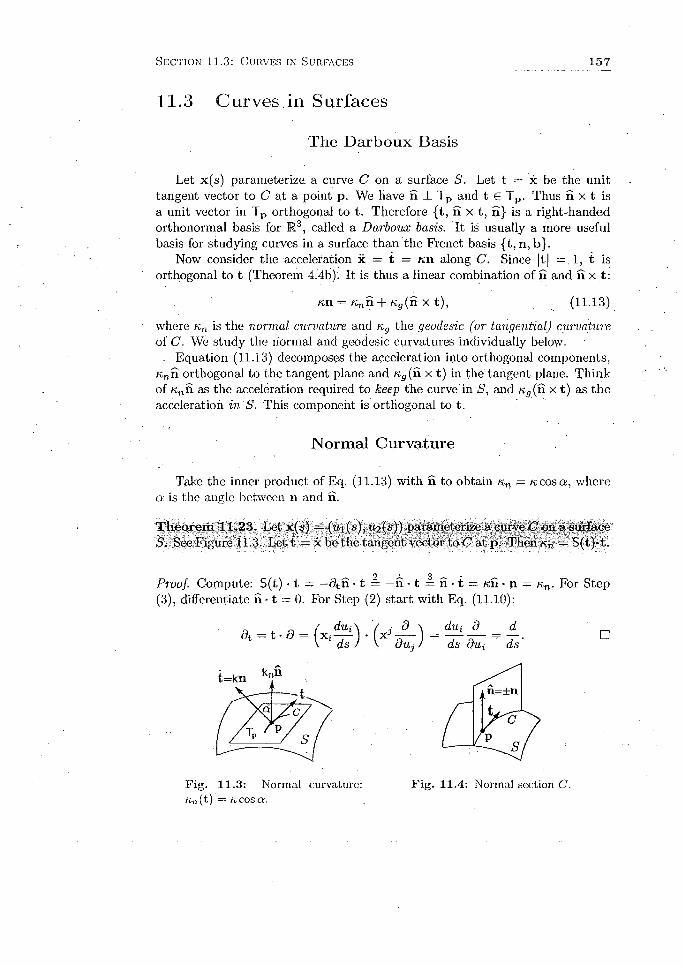
S e c t i o n 11 .3 : C u r v e s in S u r f a c e s 1 5 7

11.3 C urves in Surfaces

The D arb ou x Basis

Let x(s) parameterize, a curve C on a surface S. Let t = x be the unit tangent vector to C at a point p. We liave n _L T p and t € Tp. Thus n x t is a unit vector in Tp orthogonal to t. Therefore {t, n x t , ii} is a right-handed orthonormal basis for R3, called a Darboux basis. It is usually a more useful basis for studying curves in a surface than the Frenet basis { t,n , b}.

Now consider the acceleration x = t = /cn along C. Since |t| = 1, t is orthogonal to t (Theorem 4.4b). It is thus a linear combination of n and n x t:

«n = Knn + Kg(n x t), (11.13)

where Kn is the normal curvature and Kg the geodesic (or tangential) cui'vature of C. We study the normal and geodesic curvatures individually below.

. Equation (11.13) decomposes the acceleration into orthogonal components, K„n orthogonal to the tangent plane and Ks (n x t) in the tangent plane. Think of Knti as the acceleration required to keep the curve in S, and ng ( n x t ) as the acceleration in ' S. This component is orthogonal to t.

N orm al Curvature

Take the inner product of Eq. (11.13) with n to obtain Kn = n cos a, where a is the angle between n and n.

T h e o re m 11.23. Let x(s) = (ui(s),U2(s)) parameterize a curve C on a surface S. See Figure 11.3. Let t = x be the tangent vector to C at p. Then kt, = S(t)-t.

Proof. Compute: S(t) • t = — dt n ■ t = —n - 1 = n • t = /en • n = Kn. For Step (3), differentiate h -1 = 0. For Step (2) s ta rt with Eq. (11.10):

/ d u i \ ( ,• d \ dui d d '

= (X ) • (XX ) = °

F ig . 11 .3: Normal curvature: «n (t) = c c o s a .

F ig . 11 .4: Normal section C.

15 8 CHAPTER 11: DlDTERENTlAL G EOMETRY IN R 3

We now have nn = k co su = S(t) • t. Different curves with tangent t at p have different k and a, but they all have the same nn. Thus the normal curvature is not a property just of curves on S , but of S itself.

We discuss a special kind of normal curvature, where C arises in a special way. A plane containing the unit normal n to a surface S a t p is called a normal plane to S at p . See Figure 11.4. The normal plane.intersects S in a curve C, called a normal section. Since C is in the normal plane, so are t and n.

C o ro lla ry 11.24. For a normal section C, #t„ = ±/c.

Proof. Since n is in the normal plane and orthogonal to t , ri = ± n . ThusKn = f t COS O' = ±K. • □

We investigate nn(t) as t rotates around n at a point p on a surface.

T h eo rem 11.25. Let {ex,0 2 } be an orthonormal basis of eigenvectors of the symmetric shape operator S (spectral theorem, LAGA Theorem (9.23)). Then • Kn(e i) alld Kn(e2) are the eigenvalues of S.

Set tg = cosOei + sin #e2, the unit vector at angle 8 from e j. Then

Kn(to) = ft„(ei)cos20 + /cn(e2)sin20. ' (11.14)

If Kn (ei) > Krt(e2) (say), then Kn(tg) has a maximum in the direction ei (8 = 0°) and a minimum in the direction e 2:($ = 9GQ).

Proof. Let S(ei) = A iej. Then «n (ei) = S(e i) • e-i = Aiei - e* = Ai. Similarly, ■Kn(&2) — ^ 2- Also,

^ri(ô) S(t$) * 10

= (S(ei) • cos2# + 2 ( S ( e t ) • e 2) sin 6 cos 8 + (S(e2) • e 2)sin2#

= /c„(ei) cos2# + /in (e2) sin2#.

If Kn (ex) > Kn(e2), then from Eq. (11.14),

« n ( t « ) = K „ ( e i ) c o s 2 # + / t n ( e 2 ) ( l - c o s 2 # ) - ( / c „ ( e :l) - /en ( e 2 ) ) c o s 28 + K „ ( e 2 ) .

This lias a maximum when 0 = 0 and a minimum when 8 = tt/2. □

D efin itio n 11.26 (Principal vectors, curvatures). The eigenvectors ex and e2 of the shape.operator S are called principal vectors. Their eigenvalues Kn(ej) and Kn(^2) are called iirincipa/ curvatures. , :

E xercise 11.23. a. Determine principal vectors and curvatures at the origin for the surface z = x y 'o i Exercise 11.1.8. Perhaps you can guess them from S(i) = j and S(,j) = i.

b. Determine Kn (t«) from Eq. (1.1.14) for z — xy at the origin.c. W hat happens to h and Kn(t$) as 0 increases from 0 to tt/2.

S e c t i o n 11 .3 : C u r v e s in S u r f a c e s 1 5 9

E xerc ise 11.24. Determine principal vectors and curvatures for the torus of Exercise 11.20.

Fix p in a surface S. We show th a t the principal curvatures at p give a quadratic approximation to S near p.

Translate S so that p is at the origin. Then rotate S so that its tangent plane is the xy-plane. Rotate again so th a t the principal vector ei lies along the a;-axis. Now S is the graph of a function f ( x , y) near p.

Approximate / near (0,0) using Eq. (3.5):

f (x , y ) ~ (/zx(0,0)x2 + 2/^(0,0)xy + f yy(Q,Q)y2).

From Exercise 11.25 and S(o,o)0) = anfi similar expressions for S(o,o) (j)^

~ ^(«n(ei)a:2 + _nn (e2)y2). ; (ir.15)

If K„(ei) and nn (e2) have the same sign, then the graph of the right side is an elliptic paraboloid. Example: Figure 1.5. I t approximates S near p. If they have opposite signs, then a hyperbolic paraboloid approximates S near p . Example: Figure 6.1.

E x erc ise 11.25. Define a surface S by z. = f ( x ,y ) . The unit normal, to S is fi = (Exercise 4.12b). Give reasons for the numbered steps:

S(0,0)(i) = - f i r (0,0) = fxx(0, 0)i + fxy(0, 0)j.

Computational hint: Set Q = 1 + / 2 4- / 2 and deal with it as little as possible, remembering th a t it will be evaluated at (0,0) in the end.

G eodesic Curvature

D efin itio n 11.27 (Geodesic). A curve x(s) in a surface S is a geodesic if ng = 0.' Equivalently, from Eq. (11.13), t = Knfi.

For a geodesic, the acceleration t(s ) is parallel to fi; it has no component in the tangent space. The geodesic is “as straight as possible” , given that it is constrained to the surface. If you find yourself on a curved surface wishing to traverse a geodesic, always walk straight ahead, following t over hill and dale - no turning allowed.

E x erc ise 11.26. Show that the equator of a sphere is the only circle of latitude which is a geodesic. Hint: Use Exercise 11.2.

E x erc ise 11.27. Show th a t normal sections are geodesics.

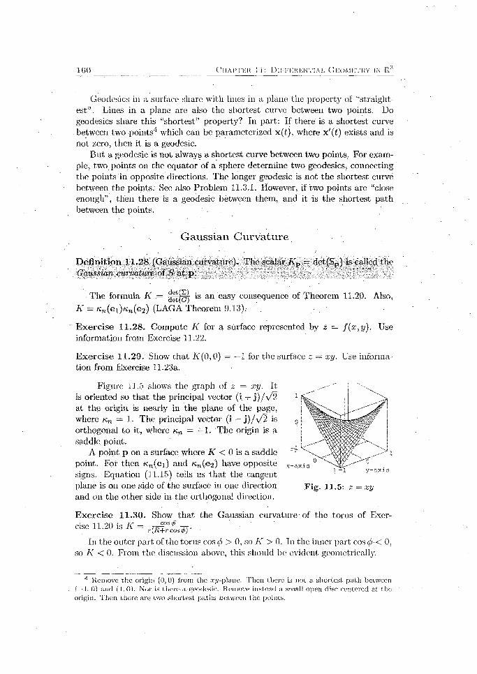
1 6 0 C h a p t e r II : D i k f b r b n t i a i . CJe o m b t r y in lit3

Geodesics in a surface share with lines in a plane the property of “straight- est” . Lines in a plane are also the shortest curve between two points. Do geodesics share this “shortest” property? In part: If there is a shortest curve between two points'1 which can be parameterized x(f), where x '(f) exists and is not zero, then it is a geodesic.

But a geodesic is not always a shortest curve between two points. For example, two points on the equator of a sphere determine two geodesics, connecting the points in opposite directions. The longer geodesic is not the shortest curve between the points: See also Problem 11.3.1. However, if two points are “close enough” , then there is a geodesic between them, and it is the shortest path between the points.

G aussian Curvature

D efin ition 11.28 (Gaussian curvature). The scalar K p = det(Sp ) is called the Gaussian curvature of S a t p.

The formula K = *]et(G) 1S an easy consequence of Theorem 11.20. Also, K = Kn(ei)Kn (e2) (LAGA Theorem 9.13).-

E x erc ise 11.28. Compute K for a surface represented by 2 = f ( x ,y ) . Use information from Exercise 11.22.

E xerc ise 11.29. Show that K ( 0,0) = —1 for the surface 2 = xy. Use information from Exercise 11.23a.

Figure 11.5 shows the graph of 2 = xy. It is oriented so that the principal vector (i + j) / \ /2 at the origin is nearly in the plane of the page, where Kn — 1. The principal vector (i — j ) / \ /2 is orthogonal to it, where nn = —1. The origin is a saddle point.

A point p on a surface where K < 0 is a saddle point. For then «n(ei) and Kn(ea) have opposite signs. Equation (11.15) tells us th a t the tangent plane is on one sido? of the surface in one direction and on the other side in- the orthogonal direction.

E xerc ise 11.30. Show th a t the Gaussian curvature of the torus of Exercise 11.20 is K = /pT08^—ryr(IZ+rcosq>)

In the outer part of the torus cos <f> > 0, so I\ > 0. I11 the inner part cos </;■< 0, so K < 0. From the discussion above, this should be evident geometrically.

4 R em ove th e origin (0 ,0 ) from th e .c.y-plane. Then there is no t a shortest p a th betw eenI .- 1. 0) ai id ( 1. 0). Nor is (.here a. g tw les ie . R em ove in s tead a sm all op en d isc cen te red a t th e

origin. T h e n th e re a r e two sh o r te s t p a th s betw een th e po in ts .

S e c t i o n 11 .3: C u r v e s in S u r f a c e s 1 6 1

E xerc ise 11.31. .Show that K = 1 / / r on a sphere of radius p. Hint: See Exercise 11.19 and LAGA Corollary 9.3.

The surface in Figure 11.6 is a surface of revolution, obtained by rotating a curve around the z-axis. (It is the graph of z = \ / l — x 2 arccosh(l/.T:).) You can see that K < 0 everywhere on the surface. In fact, I\ is constant. Because of this the surface is called a pseudosphere.

l \

Fig. 11.6: A pseudosphere. Fig. 11.7: The Gauss map .

. We now have some understanding of the geometric significance of the sign of K . W hat about its magnitude? We show th a t it is an “area magnification factor” .

D efin itio n 11.29 (Gauss map). Given a point p on a .surface translate n p parallel to itself so th a t its initial point is a t the origin. Then its terminal point is on the unit sphere. This .map from S to the unit sphere is called the Gauss map. We denote it rj.

As p moves around on S, r](p) moves around on the unit sphere. In this way a region on S is mapped to the region on the unit sphere. See the gray regions in Figure 11.7.

T h e o re m 11.30. Let x (u ,v ) parameterize a surface S. Choose a (tto,vo) and set x(uo,v0) = P- Let R$ be a small disc of radius 6 centered a t (uq, vq). Lc;t A x (Rs) be the area of n(R.s) and A ^ R g ) be the area of T}(pc(Rg)). Then

4-»o A X(R S)

Proof. n u = (xu * n u)xu + (xu - n u)x,; = - ( x u - S(xu))xu - (xu - S(xu))xv3 _ _

Step (1) is Eq. (5.22). Step (2) is Exercise 11.15. Step (3) is Exercise 11.21a. Similarly, n„ — —suvx u — s„ x „ . Thus

n u A n„ ~ ( ^ u u ^ w )xu A x 5, (dot 5 )(x u -A x^) — A (xu A x l;).

Now we arc ready:

A v (Rs) l l i f t s lIlu ^ ni,l dA __ I f / i s ^ Xl,)l dA A x (R s) f f j i s Ix« A x „| dA JJ/j J x u A x „| dA

1 0 2 C h a p t e r ll: D i f f e r e n t i a l G e o m e t r y in R 3

Step (!) is Definition 9.1. The numerator 011 the right is |A '||(xu A x„)|A(i?j) evaluated at some (u , v) & R.$ (Theorem S.8 ). The denominator is |x11AXi)|A(i?,^) evaluated at some (probably other) (u,v) £ Rg- As 5 —> 0, all quantities approach their value at (uo,vq). Thus their quotient approaches \KV\. □

We now state one of the most important results of the differential geometry of surfaces in R3.

T h e o r e m 1 1 . 3 1 . T h e G a u s s i a n c u r v a t u r e K o f a . s u r f a c e i s d e t e r m i n e d b y t h e

m e t r i c G o f t h e s u r f a c e .

We defined the Gaussian curvature K ' is in terms of the shape operator, which was defined using n. So the theorem is by 110 means obvious. We give 110

proof, as it involves lengthly calculations, a reflection of the depth of the result.The importance of the theorem goes beyoiid even this: its generalization

to higher dimensional manifolds leads to Riemannian geometry, an important branch of mathematics. General relativity, Einstein’s theory of gravity, models space and time together as a Riemannian.manifold.

Here is a specific formula for K when g12 — 0 (i.e., when Xi * x 2 — 0):

1 _ 1 1 _ 1 1 K — - (flii,922) 2 {d\ { 9 n d i922) + 92(g22 d2gil ) }.

If 312 7 0, then there is a much more complicated formula for K in terms of G.

E xerc ise 11.32. a. Parameterize a cylinder with Eq. (1.6). Show that the metric G(r,0) = [g®]-

b. Parameterize the cylinder differently so that the metric is [J ^].

A portion of a plane can be rolled into a cylinder without changing distances between points, i.e., without changing the metric. This explains why there are parameterizations of the plane and cylinder with the same metric (Exercises 11.9a and 11.32b). Gauss’ theorem then implies th a t the cylinder has the same Gaussian curvature as a plane: K = 0. We can also see this from Definition 11.28 and Exercise 11.1(5: K = — - - 0 = 0.

A cylinder s e e m s curved, so w hat’s up? The curvature cannot be detected by measurements of distances, angles, or areas i n the surface. For the rolling does not affect them. We say that the cylinder is riot i n t r in s i c a l l y curved. However, Exercise 11.16 shows that the cylinder is e x t r in s i c a l l y curved, i.e., curved in R3: — dXon = - ± x o ^ 0 .

This intrinsic/extrinsic dichotomy is important in differential geometry. As another nonobvious example, the geodesic curvature Kg is intrinsic.

E x erc ise 11.33. What, is the Gaussian curvature of a cone?

E x erc ise 11.34. Show that a map of a region of the Earth must distort distances. Take the Earth to be perfectly spherical. Make no calculations.

S e c t i o n 11.3 : C u r v e s in S u r f a c e s 1 6 3

Standard Term inology

Here is some standard terminology used in surface theory but not used here. The metric G (Eq. (11.5)) is called the first fundamental fo im of a surface. The map (u ,v ) u • S(v) is called the second fundamental form of a surface. I t appeared several times in this section.

Higher D im ensional M anifolds

The. normal vector n is pervasive in this section. It is the dual of I 2 , the pseudoscalar. of (the tangent space to) the surface. An (n-l)-dimensional m anifold in Rn has normal vectors n. Otherwise our definition of the shape operator, 'S(h) = — 3|,S, fails. But manifolds always have tangent spaces with .pseudoscalars I. •

These pseudoscalars are pervasive in the geometric calculus approach to differential geometry on manifolds. For they completely determine the geometry of the manifold.

The key is the.shape operator. It is defined by S(h) = This is abivector valued (not obvious) linear function of tangent vectors h. In general S(h) is not in the tangent space.

Unfortunately, I could not find a way to incorporate this shape operator into a book at this level. So I used the vector calculus version, limiting myself to R3.

1 6 4 CH A PT ER 11: DIFFERENTIAL GEOMETRY in IR3

P rob lem s 11.3

11.3.1. The helix x(0) = r(co s0 i + s in# j) + hdk, 0 > 0 (Exercise 7.8) is on the cylinder x{6,.z) = ?*(cos 0 i + sin 6 j) + z k (Eq. (1.6)). Show that it is a geodesic.

There are infinitely many geodesics on the cylinder connecting given points x(du zi) and x(02,z'2) if z2 z\. The idea is to start at x (6 \ ,z i ) and wind a helix around the cylinder n times before arriving at x(#2> 22 ). It is just a matter of aiming correctly.

11.3.2. Let C be a curve on a surface. Show that k2 = + /c2.

• 11.3.3. Show that nn = t(s) • n and ng = t(s) - ( n x t ) .

11.3.4. This problem is 'a continuation of Problem 11.2.8, concerning surfacesof revolution. ' ,

—ra. Use Problem 11.2.8c to show th a t K = Thus the sign of K

is the sign of — r " , which should be geometrically evident from the discussion following Exercise 11.29... b. The curves 0 = constant on a surface of revolution are called meridians.

Show th a t they are geodesics.c. The curves z = constant on a surface of revolution are called parallels.

Compute Kg for parallels using Problem 11.3.3. Recall Exercise 7.7. When is the parallel a geodesic?

11.3.5 (Euler characteristic). Show th a t JJtorusK d S = 0. See Exercise 11.30.

This is a very special case of the Gauss-Bonnet theorem.5 For a closed surface S the theorem s t a t e s th a t j f s K d S = 2nx(S), where x(S), an integer, is the Euler characteristic of S.b The Euler characteristic of a torus is zero, which gives the result. The Euler characteristic of a sphere is two, independently of its radius, so f f 3phere K d S = 4?r. This is easy to check using Exercise 11.19.

An interesting thing about the Euler characteristic is th a t it is a topological invariant, which means th a t it does not change if the surface is stretched or. twisted. Thus neither does [fs I<dS = 2irx(S) change. For example,fLaiipsiod dS = llsvhereK dS.

r,h t; tt> : / / s n . y i k l p e d i . a . o r g / w i k i / G a u s s l : . h 0 0 rorn

6 h t t p : / /e n . w i k i p e d i a . o r g / v i k i / E u i e r _ c h a . r a c t e r i s t i c

Part VI

Appendices

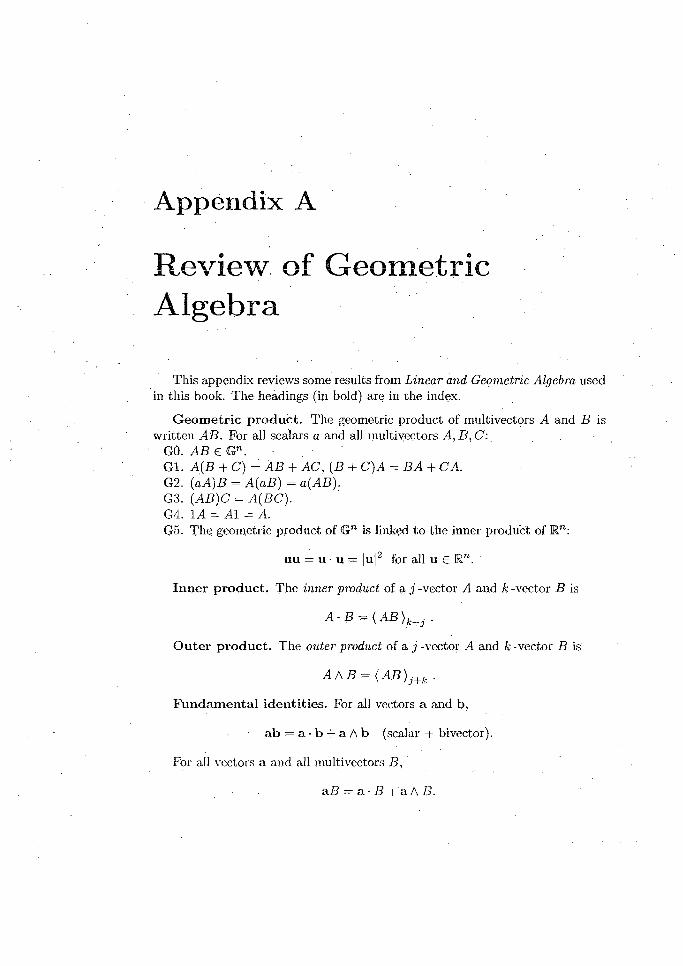
A ppendix A

Review of Geometric Algebra

This appendix reviews some results from Linear and Geometric Algebra used in this book. The headings (in bold) are in the index.

G e o m e tr ic p ro d u c t. The geometric product of multivectors A and B is written A B . For all scalars a and all multivectors A ,B ,C :

GO. A B € Gn .G l. A (B + C) = A B + AC, (B + C)A = BA + CA.G2. (aA)B = A(aB) = a(AB).G3. [a B )C = A(BC).G4. LA = A I = A.G5. The geometric product of <Gn is linked to the inner product of Kn:

u u = u • u = |u |2 for all u £ Rn.

In n e r p ro d u c t. The inner product of a j -vector A and k -vector B is

O u te r p ro d u c t. The outer product of a j -vector A and fc-vector B is

A / \ B = ( A B ) j+k -

F u n d am en ta l id en titie s . For all vectors a and b,

ab = a - b + a A b (scalar + bivector).

For all vectors a and all multivectors B,

slB — a - B + a A B.

1 6 8 C h a p t e r A: R e v i e w o f G e o m e t r i c A l g e b r a

P seu d o sca la r . If {ei e-? . . . e„} is an orthonormal basis for Kn , then the 71-vector (and blade) I = ex e2 • • • e n is a u n i t p s e u d o s c a la r . It satisfies |I| = 1.

I~1 _ (_!)"(" —1)/21_

If v is a vector, then vl = (— l)n_1Iv. More generally, if B is a A;-vector, then B I = ( — l ) k n~ lHB.

D uality . The dual of a multivector A is A* = A / I = A I ~ 1, where I is the unit pseudoscalar. The dual satisfies:

a. (aA)* = aA*. ■ ■ -b. (.4 ; /;)* A ' i i r .c. A** == ( - l ) n(n_1^ 2L4. 'd. If A is a j-blade then A* is an (n —j)-blade.e. If A represents a subspace U, then A* represents U x .

. f. |A*i A . 'g. If A is a j-vector, then 4* is an (n — j)-vector.

These duality relations are used often in this book:

• (A -B )* = A a B*,' (A f \B )* = A -B * .

The formulas are easy to memorize. It is probably worthwhile for you to do so.In R3, v** = —v, because I2 = —I.

C ross p ro d u c t . The cross product is

u X v = (u A v)*.

It is orthogonal to the plane of uAv, i.e., orthogonal to u and v, in the direction given by the right hand rule. Its norm is |u x v| = |u|jv| sin#.

L in ea r t ra n s fo rm a tio n . A function f : Rm —»■ R” is a linear transformation if f (a u ) = af(u) and f(u + v) = f(u) + f(v).

A d jo in t. The a d j o i n t of a linear transformation f : U —> V is the unique linear transformation f*: V —> U satisfying

f ( u ) - v = u -f* (v ).

O u te rm o rp h ism . Every linear transformation f: Rm —> Ra extends to a outermorphism f : G m —> Gn .satisfying f(AAB) = f(.4)Af(I?) for all multivectors A and B. ■

O p e ra to r n o rm . Let U arid V be vector spaces. The set of all linear transformations f: U h V is a vector space;. Denote it £ (U , V). If U and V are inner product spaces, define the o p e r a to r n o r m on £ (U , V):

|f|e> = max |f(u)|.| u | < l

The norm satisfies |f(u)j < |f |o |u | for all u € U.

1 6 9

D e te rm in a n ts . If f is a linear transformation on K", then.its determinant is defined by f(I) = det(f)I. It satisfies det(g o f) = det(g) det(f). If f has an inverse, then det(f-1 ) = (det(f))-1 .

deta b

— ad —be.c d

a b c - r i

d e f = a dete / — b det

d / + c detd e

h i 9 i g .h_9 h i “

E q u a tio n s o f lines a n d p lanes. Designate an origin O and consider vectors v whose tail is at the origin. These equations should be geometrically evident to you.

Line through the head of a vector vj and parallel to the vector V2 .Parameterization: v ( i ) = v i + i v 2.

Line through the heads of vectors v'i and v 2.Parameterization: v ( t ) = v 2 + t ( v \ — v 2) = t v \ + (1 — i)v 2.

Plane through the .head of a vector vo and orthogonal to a vector n. Equation: (v — v 0) • n s= 0.

R ev ers io n . The reversion M'' of the multivector M has these properties:(i) ( a j A a 2 A - - - A a j ) ^ = a 3- A - - - A a 2 A a j . Hence the name reversion.(ii) If M is of grade j , then M* =(iii) ( h h + M 2)t = M l + M l

(iv) (M iM 2)] = M \ m \.(v) (M t)t = M .

A ppendix B

Software

This appendix describes the software needed for the computer exercises and problems in this book. It has been tested on Windows.7 and Linux, but not on a Mac (yet). Please go to the book’s web site for updates on this information.

If you are not able to install the software with the directions below, please find someone to help you.

The three pieces of software you need are Python, SymPy, and GA. All are freely downloadable from the web. Python is a multiplatform computer language. SymPy is a computer algebra system written in Python. Commercial computer algebra systems include Maple and Mathematica. These systems provide symbolic computation capabilities. GA, also written in Python, provides symbolic geometric algebra and calculus capabilities.

« P y th o n . Download and install the latest version (currently 2.7.3) from h ttp :/ /w w w .p y th o n .o rg /g e t i t . (Versions 2.5 and 2.6 might work. Version 3 will not.) Full documentation is at h t tp : / /d o c s .p y th o n .o rg .

• S ym py. Download and install from h t tp : / / c o d e .g o o g le . com/p/sympy/ d o w n lo ad s /lis t. Full documentation is at h t tp :/ /d o c s .s y m p y .o rg

« G A . Download GA.zip from the book’s web page. Unzip it into the \Lib\site-packages folder of your Python installation. Also put a file GA.pth containing a single line “GA” (without the quotes) in the site- packages folder. This appendix provides documentation of the GA module for use with this book. It gives only a minimal introduction to GA sufficient to solve problems from the text. In some situations there are alternative simpler approaches to those described here. But to include them would complicate this appendix. Full documentation is in the file G A /docs/Jouild /h tm l/G A .pdf.1

« N u m P y . This is a Python’s package for serious numerical calculations. If you need it, download from h .ttp : / /s o u rc e fo rg e .n e t /p ro je c ts /n u m p y / f i l e s . Full documentation is at h t t p : / /d o c s . s c ip y . o rg /d o c /

1T h e f i le la g a .p y used w i t h L in e a r a n d G e o m e t r ic A lg e b ra is n o t needed fo r th is b o o k .

http://www.python.org/getit

http://docs.python.org

http://code

http://docs.sympy.org

http://docs

1 7 2 C h a p t e r B : S o f t w a r e

Vector Calculus

The file ”Template.py” at the book’s website provides a template for your Python programs. Remove or uncomment lines before starting with your program to suit your needs.

The first line in all SymPy programs should import SymPy: from sympy im port *

D iffe ren tia tio n , in c lu d in g p a r tia l d iffe ren tia tio n . Note that everything on a line following a is a comment.

x ,y = sym bols(’x y J) # D efine th e symbols you want to use. p r in t d iff(y * x * * 2 , x)Output: 2*x*yp r in t d i f f ( d i f f ( x * * 2 ,x ) , y ) .Output: 2*x ' •

Ja c o b ia n . Let X be a 1 x n matrix of functions of m variables, representing a function f : Mm —>• JRn . Let Y be the 1 x m matrix of the m variables. Then X. jacobian(Y ) is an n x m matrix, the matrix of the differential of X.

r , t h e t a = sym bols(’r t h e t a 1)"X = M a t r ix ( [ r * c o s ( th e ta ) , r * s in ( th e ta ) ] )Y = M a tr ix ( [ r , t h e ta ] )p r in t X. jacobian(Y ) # Print 2 x 2 Jacobian matrix.p r in t X .ja c o b ia n (Y ) .d e t() # Print Jacobian determinant. (O nly ifm = n.)

Sometimes you do not want to differentiate with respect, to all of the variables in X, for example when applying Eq. (3.26). For this, only include in Y the variables to be differentiated. For example, using Y = M a tr ix ( [ r ] ) in the example above produces the 2 x 1 matrix [ si« o 1-

In te g ra t io n .i n t e g r a t e ( f , x) returns an indefinite integral f f dx.

i n t e g r a t e ( f , (x , a , b )) returns the definite integral dx. x = Sym bolC x’) in te g ra te (x * * 2 + x + 1, x)Output: x**3/3 + x**2/2 + x

I te r a te d In teg ra ls .

This code evaluates f^_0 f* + y) dy dx: make_symbols( ’x y ’)11 = in te g ra te (x + y, (y, 0, 1-x))12 = i n t e g r a t e ( I I , (x, 0 , 1))

evalf.p r in t log(10) , log(10) ..evalf (3)Output: lo g (10) 2 .30

1 7 3

Geom etric Calculus

If you want to use the GA module of SymPy, you must import it and specify the <Gn in which you want to work. For <G3 give these commands:

from sympy import *from GA import *b a s i s = ’ e l e 2 e 3 ’

m e t r i c = ’ 1 0 0 , 0 1 0 , 0 0 1 ’

coords = (x ,y ,z ) = sym bols(’x y z ’)( e l , e 2 , e 3 , g r a d ) = M V . s e t u p ( b a s i s , m e t r i c , c o o r d s )

Now you can define multivectors, e.g, M = 3*x*y*el + 4*el*e3. These operations on multivectors are available:

+ add

- subtract

* geometric product

< inner product (as defined

A . outer product .

M.normO \M\

Mln9rm2() M 2 -

M .grade(k) ( M ) k '

M .gradeQ ( M ) oMV. I I

MV.Iinv I - 1

If you see the arithmetic expression 2 + 3 * 4 you know to multiply 3 * 4 first and then add 2 . This is because that mathematics has a convention th a t multiplication comes before addition. We say that multiplication has higher precedence than addition. If you want to add first, write (2 + 3) * 4.

For the arithmetic symbols used this book, Python’s precedences from high to low are *,H— , A, < . Plus and minus are grouped because they have the same precedence. This book’s precedences are* (geometric product), A (outer product), < (inner product), H— . The low precedence of H— causes a problem. Consider the expression e j + e 2 -e3. Python evaluates this as (ej -I- e 2) ■ e 3 = 0. If you intend ei + (e2 • e 3) = e i , in accord with the precedences of this book, then you must use parentheses.

Here are the rules to get the results you intend. Break a multivector expression into what you consider its terms. Call a term safe if it is a scalar times a geometric product of vectors. Most terms are safe or can be rewritten as safe. Fully parenthesize terms which are not safe, including parentheses around them.

Consider again the expression e i + e 2 • e,3 . If you consider its terms to be e i and e 2 • e 3 , then e_> • eg is not safe and must be rewritten (e2 • 6 3 ). If you consider it to be a single term, (ej 4 - e 2) • e^: then it is not safe, and must be written th a t way. If there are other terms, it should be written ((e t + e 2) • e3).

1 7 4 C h a p t e r B : S o f t w a r e

V. The variable grad returned from MV. se tu p above is a special “vector” which represents the gradient V.

grad is applied to functions. Functions can be defined in two ways:

A = MV(.’A’ , ’v e c to r ’ , fc t=T rue)A = x + y*el + (z* e l A e2)

The first line creates a general vector valued function on M3 with arbitrary coefficients. The possible grades are s c a la r , v ec to r, b iv e c to r , sp ih o r (even multivector - see Problem. 42.4), and mv (general multivector). ;

The second line creates a specific multivector valued function. (If e i and eo are orthogonal, then ‘A’ can be replaced with V , and the parentheses removed.)

Now we can compute the gradient, divergence, and curl-of A:

grad * A, grad < A, grad AA. .

Sometimes you want to substitute specific values in a function:

(grad A A ) .s u b s ({ x : l ,y :2 ,z :3 } )

D ire c tio n a l D e riv a tiv e .(h i , h2, h3) = sym bols(’h i h2 h3 ’ )h = h i* e l + h2*e2 + h3*e3p r in t ’D ire c t io n a l d e r iv a t iv e = ’ , DD(h,A)

C u rv il in e a r C o o rd in a te s . Curvilinear coordinates must be defined before they can be used:

coords = (r h o ,p h i , th e ta ) = sym bo ls(’rho ph i t h e t a ’ ) curv = \

[ r h o * s in (p h i)* c o s ( th e ta ) , r h o * s in ( p h i ) * s in ( th e ta ) , rh o * c o s (p h i) ] , [1 , rh o , rh o * s in (p h i) ]

( e rh o ,e p h i ,e th e ta ,g r a d ) = \ ’M V.setup(’e j:h o e_phi e _ th e ta ’ , m e tr ic , coords, curv=curv)

The two single i!\ ” characters designate a line continuation. Python does not require a “\ ” for the other line continuation. (But it is permitted there.) I used line continuations because of the length of lines in this book. You might not need them in your Python programs.

The first part of curv defines spherical coordinates (Eq. (1.10)). The second part specifies that |x^j = 1, |x^| = p, |x#| = psin<f> {Exercise 5.23a).

Now proceed with grad as before.

R ec ip ro ca l Basis., (xu r, x v r, xwr) = ReciprocalFram e(xu,xv,xw ) returns the reciprocal basis of (x u ,xv ,x w ) in (xur, xvr, xwr). Sometimes the denominator in Eq. (5.20) is so complicated that when dividing by it SviiiPy makes a mess, (xu r, x v r, xwr, Esq) = R ecip rocalF ram e((xu ,xv ,xw ), ’unnorm’) returns the numerators of Eq. (5.20) in (xur, xvr, xwr) and the denominator in Esq.

M anifolds

To do geom etric calculus on a manifold im p o rt a th ird module:

from sympy import *

from GA import *

from Manifold import *

Then set up a Gn as described above.

Define a manifold M parameterized by x.(u,v):M v a r = ( u , v ) = s y m b o l s ( ’ u v J )

x = u * e l + v * e 2 + ( u * * 2 + v * * 2 ) * e 3

M = M a n i f o l d (x ,M v a r )

Define a field f on M: ■( x u , x v ) = M.basis

f = ( v + l ) * x u + u * * 2 * x v

Compute the vector derivative d f :M.Gra'd*f.

Compute the directional derivative dh (f): h = x u •+ xv ■M.DD(h.f).

Project f. on M:M.Proj(f).

Use this to compute a coderivative (Problem 5.5.1).

1 7 6 C h a p t e r l i : S o f t w a r e

Printing

By convention, a single underscore in output indicates a subscript and a double underscore indicates a superscript.(el,e2,e3) = MV.setup(’e_l e_2 e_3’, metric)

A = MV(’A’,’vector’)

print ’A = ’, A

Output: A = A__l*e_l + A_2*e_2 + A__3*e_3 The coefficients are superscripted by convention. Notice that el is used in the left side of the first line and e_l on the right, el is the variable name used in the program. e_l is what is printed.

There are three options for improving the looks of the output of p r in t statements: (i) Fmt,.(ii) enhanced printing for console.output, and (iii) L'TgX output compiled to a pdf file.

F m t. The command Fmt (n) specifies how multivectors are split over lines when printing:

n = I: The entire multivector is printed on one line. (The default.) n = 2:; Each grade of the multivector is printed on one line, n = 3: Each component of the multivector is printed on one line The n = 2 and h = 3 options are useful when a multivector will not fit

on one line. If the code A.Fmt(n) is executed, then A will print as specified. If A.FmtCn, ’A’) is executed, the string !A = ’ will print, followed by A, as specified. You can print a variable with one n and later with another.

E n h a n c e d p rin tin g . If you are sending your output to a console window, i.e. you are not using the output described below, then you may issue thestatement

enh.ance_pr int ( )

after the NV.setup statement. Then bases are printed in blue, functions in red, and derivative operators in cyan, making the output more readable.

To set this up in Windows you must tell Geany to use a special console program in GA.zip. Go to Edit/Preferences/Tools/Termiiial. Navigate to and select

Lib\site-packages\GA\dependencies\x32\ansicon.exe or Lib\site-packages\GA\dependeueies\x64\ansicon.exe,

according as you are running a 32- or 64-bit system.On Linux you need do nothing.

1 7 7

E^TgpC o u tp u t . If you have an appropriate system 011 your computer,2then output from Python print statements can be sent to a tex file and autom atically compiled and displayed 011 a pdf reader, with beautiful L'T^X typesetting. It is helpful, but not necessary, to know a bit of I T rjX for this.

.KTjny'v printing is triggered a by Format () statement after the import sta te ments. Then the last statement in your program must then be x d v iO . On Windows, the pdf output is opened in the associated pdf reader. O11 Linux, it is opened in the standard evince pdf reader.

Here is an example of this capability. When printing a.string, an underscore designates a subscript. A caret (not a double underscore) designates a

superscript.. p r in t ’\\alpha_l\\bm {X }/ \\gamma_r~3’

Output: ckjX /7 f..

The file Symbols.pdf, available at the book’s website, is a listing of common J-MJjjX symbols. The symbols there are preceded with a They can beprinted from-your Python programs by preceding them with a second' “\ ”, as in the example. -

■ This example prints some geometric algebra/calculus symbols: p r in t . 1\\b m \\n a b la , \\w edge, \ \ c d o t ’ \ \ p a r t i a l , \ . \b m \\p a r t ia l ’■' Output: V, A, •, d, d

111 L'TjrjX mode, the statement p r i n t ’ A =J , A from the beginning of this heading produces the output A — A1 ] -(- A2e 2 4- .43e,3. The coefficients are superscripted by convention.

This extends:(ax, bx) = sym bols(’a_x, b_x')- Then ax and bx print with subscripts.(ax , bx) = sym bols( ’a__x, b_jcJ ). Then ax and bx print with superscripts.

2T ex Live is know n to work , a s is M ikTex on W indow s.

A ppendix C

Formulas

First order Taylor expansion, Eq. (3.2):

/ ( x + h ) = / (x ) + d i f (x) li, + | % / ( x + t*h)hihj.

Differential, Eq. (3.6): f*(h) = /t,9tf(x).

Jacobian matrix, Eq. (3.11): '

\ d h dA . . d f x l

d x \ d x 2 QnrU.L jji

d h d h d h

d x v dx-> O'Xm

d f n d f n d f n

-d x i dx2

Chain rule, Eq. (3.13): (g o f) ' = g ' o f '; Eq. (3.14): (g o f)^ = g'f(x)f ' .

Directional derivative, Eq. (3.23): <9hf(x) — lim ^

Differential = Directional derivative, Eq. (3.24): < 9 h f ( x ) = f * ( h ) .

Gradient, Eq. (5.1): V F (x ) = eidi.F(x.).

Eq, (5.2): S h f ( x ) = ( h • V) f ( x )

Gradient = Divergence + Curl, Eq. (5.3): V.F = V • F + V A F.

Theorem 5.9: ■ '

a. V A (V A F) = 0. (The curl of a curl is zero.)b. V A (V /) = 0. (The curl of the gradient of a scalar field is zero.)c. V • (V • F) = 0. (The divergence of a divergence is zero.)d. (V A V ) F = 0.

1 8 0 CH A PT ER ( ' : 1‘OR M I !L AS

Curvilinear coordinate bases, Eq. (5. Hi):

Vector derivative, Eq. (5.23): d = x udu + x vdv.

Path integral, Eq. (7.3): (c F d s — Jja fcj.F(x(t))|x'(Z)|<jf.

Line integral, Eq. (7.9): f c F d s = Jja ^ F (x ( t )) x '( i ) dt.

Change of variables, Eq. (8,5):

Surface integral, Eq. (9-1): f f s F d S = f f A F (x (u ,v )) . \xu(u ,v )A x v(u,v)\dA.

Flux integral, Eq. (9-5): f j s F d S — f f A F (x (u . i ’)) ( x u (m, t j) A x v(u, xif^dA.

d a = dS* integral (M3). Eq. (9.8): JJs F d a = f j A F (x ) (xu x x v)dA.

Corollary, Eq. (9.9): f f s f ■ d a = f f A f (x) • (xu x x v) dA.

Directed integral, Eq. (10.2): JM dmx F = f 4(xUl A x„2 • ■ - A • ■ • x Um) d A F .

Divergence (Gauss’) theorem, Eq. (10.8): J]jv V - f dV = </|>s f - da.

Curl (Stokes’) theorem, Eq. (10.12): f f s (V x f) • da = <fic f - ds.

Green’s theorem, Eq. (10.15): f f R(dxQ — dyP)d.A = <fc (Pdx + Qdy).

Curve theorem, Eq. (10.18): f c Vcp • ds = <j)(x2 ) — ^ (x j).

Frenet-Serret equations, Eq. (11.1): t = ztn, n = r b — /tt, b = — rn .

Darboux bivector, Eq. (11.3): f l = | ( t A t + n A 11 -1- b A b) = /ctn + rn b .

Metric, Eq. (11.5), and its inverse, Eq. (11.8):

Fundamental theorem, Eq. (10.1): f Mdmx d F = §dMdm ‘x F .

G = [Sij] = [x r * ,- ]X i * X i X] * X-2

X2 * X i X 2 ‘ Xo

G~' = W 3\ = K'-x*]

Shape operator, Eq. (11.11): Sp (h) = - d hfi(p).

Darboux basis, Eq. (11.13): Kn k„S + Kg{n x t).

A ppendix D

Differential Forms

The theory of differential forms is a popular extension of vector calculus. Geometric calculus encompasses and improves this theory.1 Despite this, the transition from vector calculus to geometric calculus is easier than that from vector calculus to differential forms. This appendix compares the two formalisms.

The curl V A in geometric calculus corresponds to the exterior derivative d in differential forms. The table shows this in R 3.

Geometric calculus: V A Differential forms: d

0-vector (scalar) field

V A / = d i f ei + 9'2,/e 2 + 9,3 /e.3

0-form

df = d \ fd x \ + dofdxo + d:\fdx3

1-vector (vector) field

V A (u ie i + V2&2 + V'3 3)

= (d\V2 - d2Vi)Gi A e 2

+ ( 5 2t>3 — 33^2 )e2 A e3

+ ( 3 3Vi - d iv 3 ) e 3 A e i

1-forrn

d(v\dxi -\-v2d x2 + v3dx^)

= [d\V2 — d2vi)dx\ A dx2

+{d2v3 - d3v2)dx2 A dx3

+(<93vl — dxV3)dx3 A dxi

2-vector (bivector) field

V A ( B 12 9 ! A e 2 + B23e2 A e 3

+ Bsi&i A ei)

= (diB-23 + ^ 2 ^ 3 1 + $ 3 ^ 1 2 )

e ! A e 2 A e 3

2-form

d (B \2dxi A dx,2 4- B 23dx2 A dx 3

+ B-ndx3 A dx 1 )

— (^1^23 + &2B 31 -f- d-jB^) dx\ A dx, 2 A dx 3

3-vector (trivector) field

V A (Ti23 e j A e 2 A e3) = 0

3-form

' d(Ti23 dx,i A dx,2 A dx3) = 0

Correspondence between V A and d.

l D. H es ten es a n d G. S obczyk have a rgued th e sup e r io r i ty of g eom etr ic calculus over d if feren tia l fo rm s ( Clifford. A lgebra to G eo m etr ic Calculus, D. Reidel, D o rd rec h t H olland 1984,Sec tion 6.4.)

1 8 2 C h a p t e r D : D i f f e r e n t i a l F o r m s

Differential forms lias only the d operator. Geometric calculus lias V A, V -, and their sum V .

In differential form theory, integrals over a manifold M are of the form f M f {dxi A ... A dxm), where / is a scalar valued function defined on M. The result is a scalar. In geometric calculus directed integrals over a manifold M are of the form f M F dmx = fM F (dx.i A ... A d x ^ ), where F is a multivector valued function defined on M . The result is a multivector. The infinitesimal dmx has a geometric interpretation as an infinitesimal pseudoscalar tangent to M . ' . ' '

.Section 1.0.4 indicated how geometric calculus extends complex variable theory to higher dimensions. Differential forms provides no such extension.

Index

B - A, 14 K , 160'G», 52 .h. 146 n, 129 V , 58V 2, 134 .Vjif, 76 8 , 75 f ' , 151 £>30d(x,y) on d(u,v) ’

i, j, k, 4f f fv F d V , 113

H a F '/ A - 109JIs, F d < T > 122[L F d S , 119

f f s 121f G F d s , 91

F ds. 95

J t f dx, 88 k , 145 K g , 157K n , 10 i

£ (U ,V ), 168 n, 146, 153 § , 132 §, 99 8 M ,1 2 Tdh, directional derivative

K", 39 surface, 152

dtF, 23 du, 75

duv, 81 da, 28

■i£.23t , 146 Tp , 53 n, 4, 153 • x k , 69 Xj, 69 x u, 53 - dmx, 128 ■ dmx, 128' fxx 24/zy, 26 ,

adjoint, 59, 62, 168 analytic function, 141 angular momentum, 104 angular velocity, 51 antiderivative, 89 arclength, 93 axial vector, 63

binormal vector, 146 boundary, 128 boundary values, 142 bounded function, 88 bounded set, 77

Cauchy’s integral formula, 142central force, 104chain rule, 34change of variables, 115.circulation, 96, 138closed

curve, 99 field, 107

interval, 14 manifold, 130 set, 14 surface, IOC

coderivative, 76 complement, 14 congruent, 147 connected set, 19 conservation

angular momentum, 104 energy, 1.03

conservative field, 100 continuous function, 18 continuously differentiable, 31 contractible

closed curve, 102 closed surface, 106 • ■

coordinate curve, 71 coordinate surface, 71 Coulomb force, 101 cross-product, 168 curl, 60, 67 curl theorem, 136 curvature, 145 curve, 48curvilinear coordinates, 11, 60

orthogonal, 72 cylindrical coordinates, 11, 72

Darboux basis, 157 Darboux bivector, 147 De Morgan’s laws, 14 derivative

differential, 30 directional, 39, 59, 65, 152 gradient, 58 partial, 23 vector, 75, 76, 127

determinant, 169 diameter, 109 differentiable function, 30 differential, 30, 151 differential forms, vii, 18.1 differential geometry, 145 directed integral, 129 divergence, 60, 67

divergence theorem, 132 dual, 168 duality, 168

elasticity, 27 electromagnetic field, 64 electromagnetic waves, 64 electromagnetism, 63 entropy, 84equation of continuity, 135 equations of lines and planes, 169 Euler characteristic, 164 even subalgebra, 52 exact

differential equation, 105 field, 107

field, 57first, fundamental -form, 163 fluids, 96, 123, 135 flux, 123, 133 formulas, 179 Frenet basis, 146 Frenet-Serret equations, 146 fundamental identities, 167 fundamental theorem

scalar calculus, 89 geometric calculus, 127

Gauss map, 161 Gauss’ theorem, 132 Gauss-Bonnet theorem, 164 Gaussian curvature, 160 geodesic, 159 geodesic curvature, 157 geodesic normal vector, 157 geometric calculus, 3 geometric product, 167 ■GPS, 44gradient, 23, 58, 70

and linear transformations, 68 Green’s identities, 134 Green’s theorem, 139

harmonic function; 142 liessian matrix, 78

1 8 4

homogeneous function, 37

ideal gas law, 38 implicit differentiation, 43 indefinite integral, 89 inner product, 167 integrable, 88 integral

definite, 88 . directed, 121, 127 double, 109 flux, 121how to think about, 90 iterated, 111' line, 95. path, 91 scalar, 87, 88 surface, 119 triple, 113 . ■

integrand, 90'intermediate value theorem, 19inverse function theorem, 41irrotational, 67isobars, 7 •isotherms, 7iterated integral, 111

Jacobian determinant, 32, 115 Jacobian matrix, 32

Kepler’s laws, 104 kinetic energy, 103 .

Lagrange multiplier, 82 Laplacian, 64, 134, 14.2 least squares, 81 level curve, 7 level surface, 66 limit, 15linear transformation, 1.68 local maximum, 77, 78 local minimum, 77, 78

Mobius strip, 76 manifold, 47manifold with boundary, 47 maximum entropy, 84

maximum uncertainty, 84 Maxwell relation, 26 •Maxwell’s equation, 64 Maxwell’s equations, 63, 106, 134 mean value theorem

integral, 110 scalar, 27 vector, 38

meridians, 164 metric, 94, 150 mixed partials, 25 multiple integral, 114

neighborhood, 13.Newton’s law of gravitation, 101, 103,

104Newton’s second law, 103, 104 normal curvature, 157 normal plane, 157 normal section, 157, 158 normal vector

/ ( x ) = c representation, 66 z = f ( x , y) representation, 54 outward boundary, 129 parameterized surface, 53 to curve, 146 to surface, 129

notation, 4

openinerval, 14 set, 13

operator norm, 168 orientable surface, 76 orientation, 129 orthogonal complement

Gn , 168 orthogonal coordinates, 72 osculating plane, 147 outer product, 167 outermorphism, 168 outward normal vector, 129

parallels, 164 parameter, 5 parameter space, 48

param eter izearclength, 93 curve, 5 surface, 8

partial derivative, 23 partition

area, 109 interval, 87

path independence, 99 . path integral, 91 pitch, 93 planimeter, 139 polar coordinates, 11 positive definite matrix, 78 potential

field, 107 scalar, 100 vector, 105

potential energy, 103 precedence, 173 . principal curvatures, 158 principal vectors, 158 pseudoscalar, 168 pseudosphere, 161 pseudovector, 63

reciprocal basis, 69, 73 reversion, 52, 169 Riemann sum, 87 Riemannian geometry, 162 rotational velocity, 51

saddle point, 79 scalar calculus, 3 scalar functions, 3 scalar potential, 100 second fundamental form, 163 shape operator, 153 simply connected, 102 Simpson’s rule, 80 software, 171solenoidal field, 106, 137, 140 solid, 48spacetime geometric algebra, 64 .spherical coordinates, 11, 72 Stokes’ theorem, 13(5

summation convention, 1 surface, 48 surface integral, 119 surface of revolution, 156, 164 SymPy, 171

tangent space curve, 49 manifold, 55

. surface, 53 tangent vector

curve, 49 surface, 53 unit, 93 ■ -

Taylor expansion, 28 tensors, viitopological invariant, 164 torsion, 146 trapezoidal rule, 89 , twisted cubic, 149

uncertainty, 84

vector calculus, 3 vector potential, 105

wave equation, 37 Weingarten equation, 1.54 Wolfram Matliematica Online Integra

tor, 89work, 96

1 8 6

Documents

Vector Calculus marsden