VcDemo Application Help - Inriapeople.rennes.inria.fr/Aline.Roumy/teaching/VCDEMO.pdf · VCDEMO.rtf VcDemo Application Help Page 2 of 55 . ... The Image and Video Compression Learning

VCDEMO.rtf VcDemo Application Help Page 1 of 55

Contents


About VcDemo (Version 5.03):

The Image and Video Compression Learning Tool Image compression modules:

SS Subsampling of images PCM Pulse-coded modulation coding of images DPCM Differential pulse-coded modulation coding of images VQ Vector quantization of images FRAC Fractal image coding DCT DCT-based transform coding of images JPEG JPEG image compression standard SBC Subband (wavelet) coding of images EZW Embedded zero-tree wavelet coding of images SPIHT Set partitioning in hierarchical trees coding of images JPEG2000 JPEG-2000 image compression standard

Video compression modules: VPLAY Video sequence player ME Motion estimation in video sequences MPEGENC Mpeg video encoder MPEGDEC Mpeg video decoder and channel simulator H264ENC H.264 video encoder H264DEC H.264 video decoder

Other features of VcDemo on which help is available Tips and Tricks Enlarging Images Subtracting images Plotting rate-distortion graphs for images About the VcDemo software development project

Quick tour of VcDemo The VcDemo image and video compression learning tool is a fully menu-driven package. It is operated by selecting compression techniques and parameters using buttons. In most cases you should be able to run VcDemo without any further explanations starting from the main application window. The main application window is shown below. Your main window may look different, depending on which release you have (usually the main application window will have more options than shown in this tour).


The purpose of VcDemo is to be able to experiment with different (sometimes very complex) image compression algorithms without bothering about their actual implementation. For this reason VcDemo is menu driven, and allows the user to experiment with different parameters that define the specific compression operations, e.g. in PCM compression what number of bits to use, and whether or not to apply dithering. On one hand visualization of image compression results will help to gain insight in "how good" a compression algorithm performs. On the other hand the compression results will stimulate a problem-solving attitude. A generally effective attitude toward using VcDemo is asking yourself all the time the questions “what will happen given a certain combination of parameters”, “what is the cause of a certain compression artifacts”, and “how do compression techniques compare visually and numerically”. VcDemo is a tool assisting the learning process, but does in itself not explain the compression techniques. Lecture materials (sheets) for a full course on signal, image and video compression is available from the author’s website: http://ict.ewi.tudelft.nl/~inald. The VcDemo software, including sample images and sequences, can be downloaded from http://ict.ewi.tudelft.nl/vcdemo. After starting, VcDemo, an image needs to be loaded to work upon. Clicking on “File-> Open Image” or on the toolbar button will give the contents of the selected image directory. Pick any bmp image, but be aware that some compression methods are restricted to image dimensions that are even, or powers of 2. A good choice is an image of 256x256 pixels, as this can be used with all compression algorithms, will and will nicely fit in the workspace. Larger images can be used, but they are sometimes shown in smaller windows because lack of space (try to double click the left mouse button in the image and see what happens!). Of course the windows of these larger images can always be resized to see them completely. VcDemo can load color or paletted images. All compression routines on images work, however, on 8 bit gray value images, so internally the input image format is converted to 256 gray values. For sequences (MPEG, H264) this may be different. After loading an image, the main application window looks like this.


This opened – usually original – image is called the “start image”, as all compression operations will work on this image. Multiple images can be open at the same time but only one image can be the start image. Results from compression operations can themselves be promoted to be a start image, so that concatenated compression can be carried out (use right mouse button in the image to open this menu). You can load different images at the same time, hence multiple start (and compressed) images can be present in the workspace. This will, however, clutter the workspace somewhat. On the toolbar, the pull-down menu, and the buttons all compression options are now visible. If some of the compression options are not active, this is due to the dimensions of the currently active start image, or because of the image type (still image, video sequence, compressed bit stream). Clicking one of the compression techniques will open the parameter menu pop-up. The menu is always positions on the right of the workspace and is immovable. The illustration below shows the result of clicking the DPCM button. The menu consists of a number of “tabs” that can be clicked. Each of the tabs contains parameters that the user can control. After clicking “Apply” the compression will be carried out using the current setting of these parameters. With “Cancel” the menu will disappear, but all resulting images obtained will stay in the workspace.


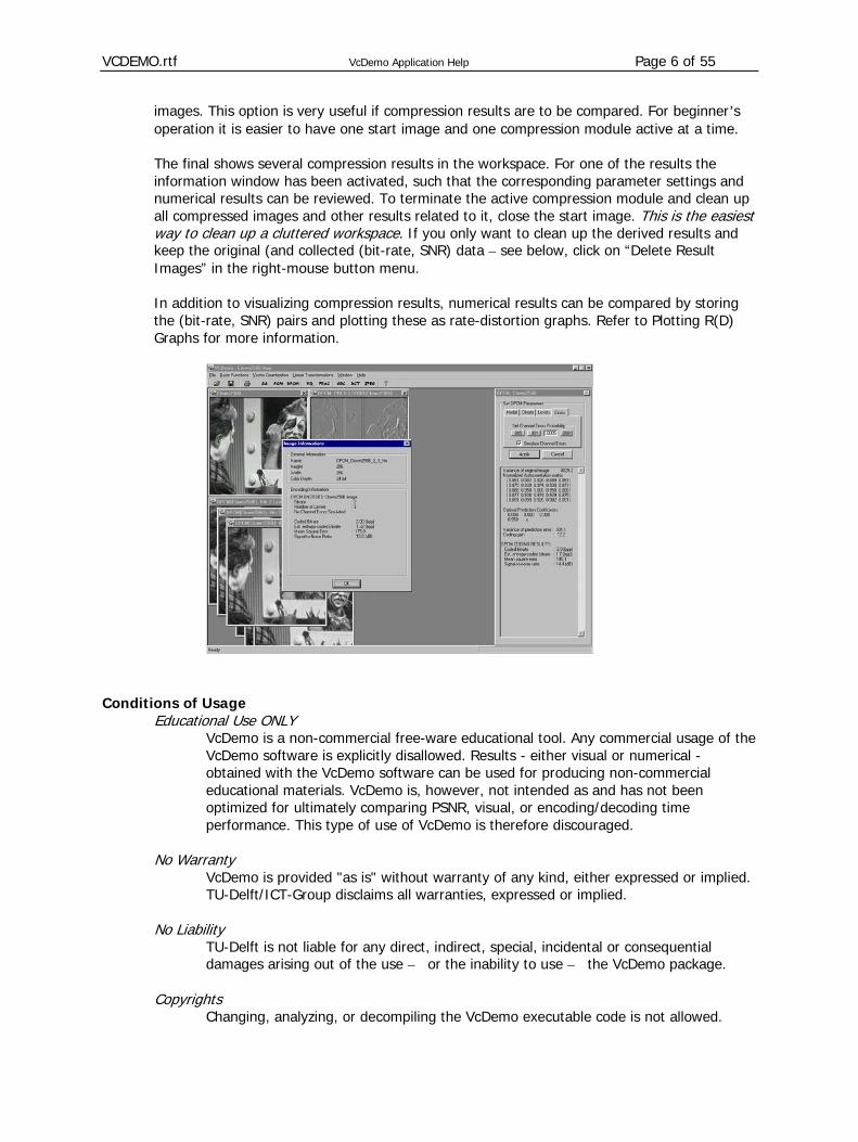
The lower part of the menu has a text window that will show numerical results of the compression, such as bit rate, signal-to-noise ration (peak-SNR and variance-based SNR). The results shown in this text window are also saved for each compressed image shown in the workspace. This information is reached by clicking in an image on the right mouse button, followed by clicking on “Image Information”.

The following figure gives the resulting configuration after pushing “Apply” for DPCM compression. In general the start image is positioned in the upper left corner of the workspace. The compressed and decompressed image is shown below the start image, in a staggered fashion. Other output results, such as spectra, DCT coefficients, or – here in DPCM compression – the prediction difference are shown to the right of the start image. This figure also shows the right-mouse button menu. From this menu, images can be saved and can be set as start image. Image compression menu’s can also directly be started from the right mouse button menu; notice that compression modules started in this way still refer to the actual start image, not to the (compressed) image in which the compression module is started.

Multiple compression modules can be active, and can refer to the same or to different start


images. This option is very useful if compression results are to be compared. For beginner’s operation it is easier to have one start image and one compression module active at a time.

The final shows several compression results in the workspace. For one of the results the information window has been activated, such that the corresponding parameter settings and numerical results can be reviewed. To terminate the active compression module and clean up all compressed images and other results related to it, close the start image. This is the easiest way to clean up a cluttered workspace. If you only want to clean up the derived results and keep the original (and collected (bit-rate, SNR) data – see below, click on “Delete Result Images” in the right-mouse button menu. In addition to visualizing compression results, numerical results can be compared by storing the (bit-rate, SNR) pairs and plotting these as rate-distortion graphs. Refer to Plotting R(D) Graphs for more information.

Conditions of Usage Educational Use ONLY

VcDemo is a non-commercial free-ware educational tool. Any commercial usage of the VcDemo software is explicitly disallowed. Results - either visual or numerical - obtained with the VcDemo software can be used for producing non-commercial educational materials. VcDemo is, however, not intended as and has not been optimized for ultimately comparing PSNR, visual, or encoding/decoding time performance. This type of use of VcDemo is therefore discouraged.

No Warranty

VcDemo is provided "as is" without warranty of any kind, either expressed or implied. TU-Delft/ICT-Group disclaims all warranties, expressed or implied.

No Liability

TU-Delft is not liable for any direct, indirect, special, incidental or consequential damages arising out of the use – or the inability to use – the VcDemo package.

Copyrights

Changing, analyzing, or decompiling the VcDemo executable code is not allowed.


Copyrights to the VcDemo user interface is held by TU-Delft/ICT Group. Copyrights of software code used in certain compression is held by third parties (see credit in VcDemo program).

Acceptance

Downloading and/or installing the VcDemo software implies agreement on the above terms of use, and in particular agreement on the restriction to educational use only.

Information and Communication Theory Group, Delft University of Technology, The Netherlands

Tips and Tricks Press F1 Activate the context-dependent help. Help can be obtained on all

menu items, images and the compression modules.

Toolbar -> Settings Allows you to change the default directory for images and user output. This might be handy is you put all you images and sequences in another than the standard directory. This option also allows for changing (some of) VcDemo’s fonts. Use this option only if you have problems with the default fonts being used in your windows version.

Left mouse button double click in image

This shows an image at its true size. Large images are usually scaled to fit them in the work area.

Right mouse button in image Shows the context dependent menu, which gives access to information about the image in which you clicked. This is handy to figure out which parameter settings were used for a particular result. You can also save an image in this way as bmp file.

Drag bottom right image corner

To enlarge/shrink images

Click X in the upper right hand corner of the start image

To close the start image and all the derived results.

Computation takes long time Use a smaller image. Your PC is probably not the fastest in the world or your machine has less than 128 MByte RAM. Alternatively, close VcDemo and start it again. If this helps, you found a memory leak in VcDemo. Please report this problem to the author.

Hit any key … To interrupt the compression, decompression, or motion estimation process on image sequences.

Click on a module button .. … if you had already activated it before, but activated a second module later on. The first module still lives, but is hidden behind the


second one. If you click the button corresponding to the first one, it will pop-up and come to the foreground.

Modules cannot be activated Some modules require particular image sizes, usually powers of 2 or even number of columns/rows. If a module is not active, than the image that you loaded has a funny size. Crop the image to another size.

Work space becomes cluttered with too many images

Close the start image (press X in the top right corner of the image), and the start image and all derived results will disappear. The disadvantage is that also stored (bit-rate, SNR) pairs are lost in this way. As an alternative, select “Delete Result Images” from the right mouse button menu, which will only delete the derived result images, keeping the start image and stored (bit-rate, SNR) pairs.


Enlarging Images Images can be enlarged by dragging the bottom right corner. The interpolation procedure used is bilinear interpolation. To display the images at their natural size – meaning that one image pixel is mapped exactly to one screen pixel – double click the left mouse button in the image to be shown at natural size.


Video Player (VPLY) If you have loaded a YUV video sequence or a sequence of BMP images, the video player module can be used to show moving video. The video player uses a fixed frame rate of (approximately) 25 frames/second.



Plotting Rate-Distortion Graphs (R(D)) When working with images in VcDemo, you can generate a lot of (P)-SNR – bitrate measurements. These pairs can be used to manually draw bit-rate versus distortion, called R(D), curves. VcDemo includes the possibility to store series of R(D) pairs and to plot one or multiple series in a graph. These graphs can be saved using a screen capture program (usually yielding a bmp file), or by writing the graph to a (encapsulated) post script (eps or ps) file. These files can be printed or included in other applications or word processing programs.

The procedure to obtain R(D) graphs is as follows: 1. Load an image and open a compression module. 2. Enable the saving of R(D) pairs. 3. Generate a series of R(D) pairs. 4. Stop saving of R(D) pairs. 5. Open plotting module. 6. Select and plot a particular series of R(D) pairs. 7. Save the R(D) graph using a capture screen program or using the write-to-postscript file

option. Saving Series of R(D) pairs

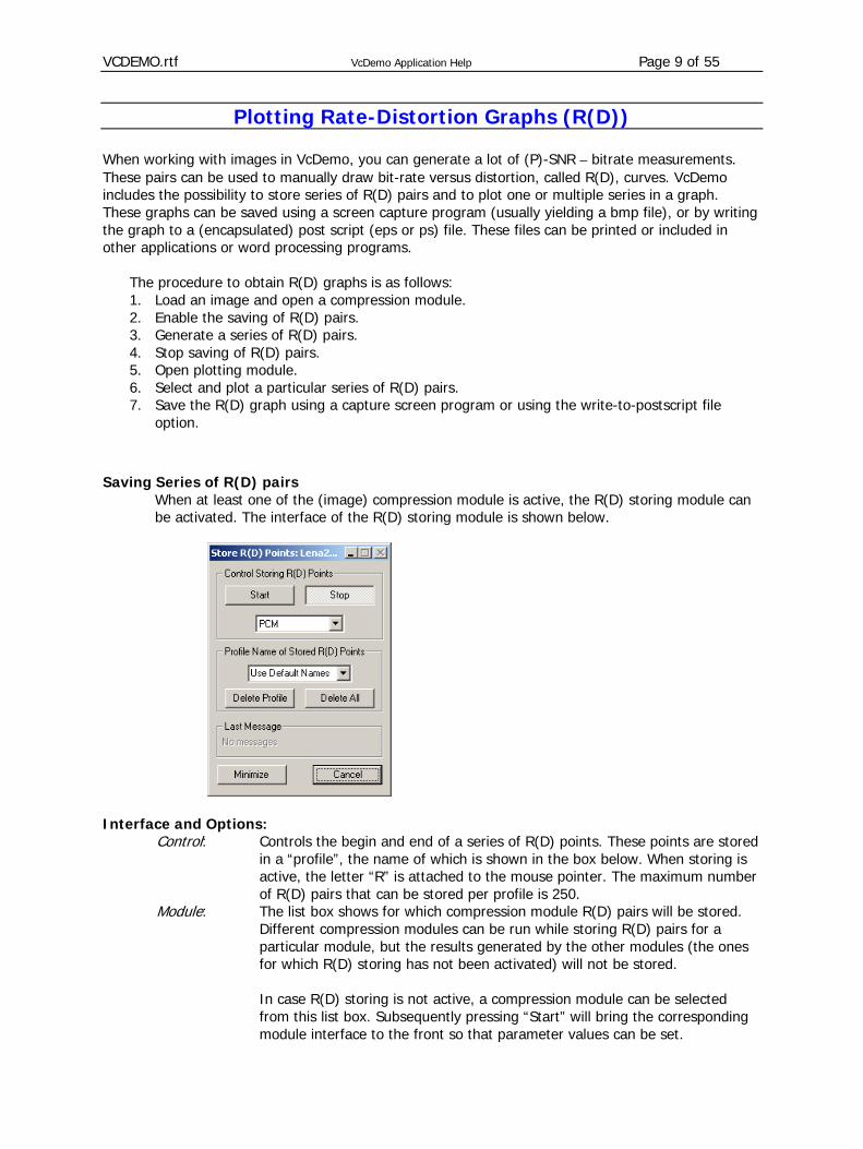
When at least one of the (image) compression module is active, the R(D) storing module can be activated. The interface of the R(D) storing module is shown below.

Interface and Options:

Control: Controls the begin and end of a series of R(D) points. These points are stored in a “profile”, the name of which is shown in the box below. When storing is active, the letter “R” is attached to the mouse pointer. The maximum number of R(D) pairs that can be stored per profile is 250.

Module: The list box shows for which compression module R(D) pairs will be stored. Different compression modules can be run while storing R(D) pairs for a particular module, but the results generated by the other modules (the ones for which R(D) storing has not been activated) will not be stored.

In case R(D) storing is not active, a compression module can be selected

from this list box. Subsequently pressing “Start” will bring the corresponding module interface to the front so that parameter values can be set.


Profile name: A profile name is associated to a series of R(D) pairs. The use can type any

name, or let the module automatically generate default names such as PCM_001, PCM_002, VQ_020. Names can only be set when storing is not active. Individual or all profiles can be deleted.

Messages: This status line gives information about the last R(D) pair stored or other

relevant information for the storing process. Minimize: When the R(D) storing module is closed (press cancel), all stored profiles will

remain in memory until the start image is closed. Alternatively, the R(D) storing module can be minimized to move it out of view. The R(D) storing module will always be the top most window of all applications. Use “minimize” to move it out of the way without closing it.

Mouse key: Clicking the right mouse key in the active R(D) storing module will give access

to an overview menu of stored profiles. The profile data (i.e. all R(D) pairs) can be stored in a text-formatted file for future reference.

Plotting R(D) graphs

Once one or more series of R(D) pairs (“profiles”) have been stored, they can be plotted in a R(D) graph using the “R(D) plot module”. The interface of the R(D) plotting module is shown below.


Show graph: The profile shown in the list box will be plotted as a new graph when pressing “Show New Graph” or added to the current graph when pressing “Add Another Graph”.


Axes’ scale: The scale of the axes can be determined automatically, based on the first profile plotted, or can be set by the user.

(P)SNR: The vertical scale can be user selected to be SNR (default) or PSNR. Save as EPS: The currently shown graph can be saved as a PS or EPS file.


Template Module Compression Algorithm:

The template module is not an actual compression module. It has been included as an example for developers who contribute to VcDemo. The only useful option for the template module is that it can rotate and mirror images. It may be interesting to see if a mirrored or rotated image gives the same compression – quality as the original one.


Information about Images Displayed Clicking on the right mouse button gives access to the context menu (see below), from which the option “Image Information” can be selected.


The Image Information window gives information about the image displayed. An example is given below.

The general information in the top half of the window shows the image name and the size of the image (actual pixel size and size of the currently (stretched) displayed image). The color depth of the image is also shown, but this is always 24 bits because of the way VcDemo deals with images internally. The bottom half gives information about the encoding process that resulted in the image being displayed. The type of information depends on the compression module, but is similar to the input and output information showed in the modules interface.


Saving Images and Decoded Video Sequences Images

VcDemo can open and save results as tif or bmp images. Images can be opened via File Open Image. Compression results can be saved by clicking the right mouse button – opening the context menu – and (at the bottom of the list), select the option “Save Image As …”.


Image Sequences

The MPEG and H.264 decoder modules can save decoded compressed sequences as YUV files.


Subtracting Images Images belonging to the same start image can be subtracted. The procedure is as follows. In one of the two images, click on the right mouse button and select “Subtract Images -> Put Image on Stack” in the image context menu. The image that is “put on stack” is the one that serves as a reference image. Often, you will use the start images as reference image, so you will put the start image “on stack”. Other images, however, can also be “put on stack”. To subtract another image, click on the right mouse button and select “Subtract Images -> Subtract from Image on Stack” from the image context menu. As the operation says, this image is then subtracted from the image you put on stack earlier, and displayed. The gray values of the displayed difference image are stretched (stretched and offset 127 for the difference “0”) to enhance the visibility of differences. The “Image Information” (again right mouse button) gives more information about the statistics of the difference image.



Opening Images, Video Sequences, and Compressed Bit Streams Images

VcDemo can open and save results as tif or bmp images. Images can be opened via File -> Open Image. Compression results can be saved by clicking the right mouse button – opening the context menu – and (at the bottom of the list), select the option “Save Image As …”.


Image Sequences Sequences come in two flavors, namely as YUV raw data files, or as a series of bmp images.

YUV Sequences: YUV sequences contain the raw image sequences without any header.

The data is stored as a series of Y-U-V data blocks. The storage format can be luminance only, or luminance-chrominance in 4:2:0 or 4:2:2 format. With each sequence a header file must exist of the same name. For instance foo.yuv contains YUV data, of which the format is described in foo.hdr. Luminance-only sequences are contained in file with extension *.y.

The ASCII header file may start with comment lines, starting with /* Then the following numbers are expected (in this order, one line per number): • (int) number of lines • (int) number of pixels per line • (boolean) flag indicating progressive (1) or interlaced (0) format • (int) color representation: gray value (0), 4:2:2 (1), or 4:2:0 (2) • (int) number of frames

If you have a raw Y or YUV data file (for instance MPEG test sequences), just edit a simple header file with the same name and the extension .hdr, and you are ready to go. Look at the examples provided in VcDemo image directory.

BMP Sequences An BMP image sequence is called, for instance, foo1.bmp, foo2.bmp, …,

foo9.bmp, foo10.bmp, etc. The program does not have knowledge of the length of this sequence beforehand. To indicate to the program that an foo sequence exists, the images must be organized as follows:

.\foo.seq

.\foo\foo1.bmp

.\foo\foo2.bmp

.\foo\foo3.bmp etc.

Upon loading time, the program will look for files with extension *.seq, and – when selected – will load this image as the first image of the sequence. Therefore, foo.seq must be identical to foo1.bmp (just a copy with different extension). All other frames will be loaded from the subdirectory foo, until a


next image cannot be found so that the program realizes that the sequence end has been reached.

Image sequences are opened by clicking on “File->Open Sequence”. The sequences with extension *yuv, *.y or *.seq are listed and can be opened. The first frame will be shown only. The modules that work with sequences can now be activated. The motion rendering in the motion estimation module is heavily dependent on the CPU speed.

Compressed Bit Streams

VcDemo can load MPEG and H.264 streams. After loading, the corresponding decompression modules can be activated.


Using a Decoded Image as “Start Image” Any compressed image can be used as “start image”. In this way, multiple compression steps can be applied to the same data. Click on the right mouse button in the image you want to start with, and select “Set as Start Image” in the image context menu.


VcDemo Settings


The VcDemo software comes as a self-installing package. The install shield will ask for an installation directory, and suggests a default one in C:\Program Files. In this install directory, four subdirectories will be created, namely: • a directory for storing all quantization tables and filter coefficients needed by VcDemo. Normally

this will be the subdirectory \Tables of the installation directory. The files in this directory should never be touched or removed by users.

• a directory for storing vector quantization codebooks. Normally this will be the subdirectory \CodeBook of the installation directory. The vector quantization module will read and let the user write codebooks into this directory

• an image directory. VcDemo comes with several test images that are written into this directory. However, VcDemo will work with any bmp image, provided that the dimensions satisfy certain compression technique-dependent constraints (for instance, even number of rows and columns). A possible choice for this directory is the subdirectory \Images of the installation directory.

• a “results” directory, where the user-saved files (jpeg, mpeg) are stored. Selected installation directories can always be changed by clicking “HelpSetting”. The directory settings are illustrated below.

In certain language regions (like Asia), the default system fonts will not fit VcDemo’s menu’s. IN that case, the user can explicitly change the default fonts (see below). Furthermore, if the layout of numerical results in the results windows are unreadable due to poor formatting, a horizontal scroll bar can be added, usually fixing this problem.



VcDemo Displayed Images The images displayed are either still pictures, yuv/bmp image sequences or decoded mpeg/h.264 bit streams. Still pictures are always displayed and processed as gray value data, even when the image on disk is a color image. Image sequences can be color (YUV, RGB) data. More information about the images displayed can be obtained by clicking the right mouse button in an image, and selecting the option “Image Information”.



About the VcDemo Project VcDemo is the result of many years of research and teaching in image and video compression by both faculty and Ph.D. researchers of the Information and Communication Theory Group of TU-Delft. In particular Prof. Inald Lagendijk and Jan Biemond have played key roles in leading the ICT group into exploring this field. The VcDemo project originally started as a VAX/VMS/Fortran implementation, later migrating via SUN/Unix/X/C and SGI/Unix/Motif/C to the Windows/Visual C platform in 1999. Since then, Prof. Inald Lagendijk has been the main force and developer of the VcDemo software, assisted by numerous students and Ph.D.’s. The VcDemo framework and many of its compression modules have been developed at TU-Delft. Several modules are, however, largely based on third party implementations. We refer to the “Credits” section of VcDemo for further reference. In case you find bugs, errors, or in case you have suggestions about the operation/modules of VcDemo, please contact Prof. Inald Lagendijk at [email protected]. Also check on recent updates on the VcDemo website: http://ict.ewi.tudelft.nl/vcdemo.


Problem Solving The following problems have been reported to the authors of the software. Problem: The fonts that VcDemo uses are funny, too large or too small. Solution: Change the font settings under “Settings” of VcDemo. If that does not help, change the

font size of your display (right mouse button on desktop -> Properties -> Display Properties)

Problem: VcDemo reports (file) writing errors. Solution: The directory “UserOutput” in the directory where VcDemo has been installed, should be

writable for the user (the user should have write access). If this is not the case, select a user-writable directory for VcDemo to put results into. Changing the directories should be done via the “Settings” menu of VcDemo.

Problem: I want to load my own YUV files into VcDemo. Solution: Use a binary fle format. Organize the YUV or Y file in a frame by frame fashion. Per


frame, first store the Y, then the U and V component. Next, make a header file with the same name and extension *.hdr. Help on the structure of the header file can be found here.

Problem: VcDemo crashes. Solution: Don’t know. Inform the author about this problem ([email protected])


Subsampling (SS) Compression Algorithm:

The subsampling module implements the undersampling of images by a factor of 2N. Subsampling can take place with or without anti-aliasing (low-pass) filtering. Different low-pass filters can be selected. For visualization purposes, the spectrum (magnitude squares of the 2-D Fourier transform) of the (subsampled) image can be displayed.

Interface and Options: The subsampling module has the following interface:

Factor Selects the subsampling factor. The subsampled image can be shown in its subsampled form, i.e. a smaller image, or can be blown up to the original image size using simple pixel replication as interpolation procedure. A smoother interpolation of the subsampled image is obtained by enlarging the image (dragging the bottom right corner of the window).

Filter Prior to subsampling, anti-aliasing filtering is normally applied. On the filter tab,

the anti-aliasing filtering can be switched on/off, and the number of taps of the low-pass filter (number of filter coefficients) can be selected. The larger the number of filter taps, the steeper is the roll-off of the transfer function of the low-pass filter, and hence less aliasing will be present in the subsampled image.


Spectrum To get insight in the spectral behavior of subsampling, the spectrum of the subsampled (or original) image can be shown. The computation of a spectrum is an issue by itself because leakage components will show up in the spectrum. In the subsampling menu the (windowed) periodogram estimator is used, i.e. first the spatial image is rolled-off to zero using a tapering or windowing function, then the Fourier transform is calculated, and finally the magnitude squared component is calculated. The user can select the tapering window that is used to suppress leakage frequencies. Notice that the spectrum calculation is for visualization purposes only and that it does not have any influence on the actual subsampling process.

Images Displayed:

Spectrum The spectrum of the (original/subsampled) image is shown. In case the

spectrum of a subsampled image is displayed, several spectral replicas are also visible.

Subsampled image The subsampled image (or a blown-up version) is displayed.


Pulse Coded Modulation (PCM) Compression Algorithm:

The PCM compression module implements a uniform scalar quantizer. The quantizer representation levels are not entropy encoded. Hence, the number of selected bits per pixel is identical to the length of the fixed length code words (FLC).


The PCM compression module has the following interface:


Bit rate Select PCM bit rate, integers only. A uniform quantizer optimized for a uniform PDF is applied.

Dithering Prior to PCM compression, a small amount of uniformly distributed noise can be

added to the image. This causes PCM compression artifacts at low bit rates to be less objectionable. Since the noise is generated deterministically, it can be subtracted at the decoder side. This option can be switched off/on.

The amount of dither noise is controlled by the dither step size d =0.75, 1.0, 1.5,

or 2.0. If the quantizer has step size ∆, then the dither noise is uniformly distributed over the interval [ -d ∆/2, d ∆/2 ].

Errors When data becomes more and more compressed, the bits become more and

more vulnerable to channel errors. By checking the box “Simulate Channel Errors”, random bit errors will be inserted into the compressed bit stream, prior to decompression. In this way an impression can be obtained of the effects of (simple) channel errors. Different bit error probabilities can be selected, namely 0.005 (0.5% of the bits are erroneous), 0.001, 0.0005, and 0.0001.

Images Displayed:

Decoded image The decoded image is shown.


Differential Pulse Coded Modulation (DPCM) Compression Algorithm:

The DPCM compression module implements a spatially predictive compression scheme. Pixel


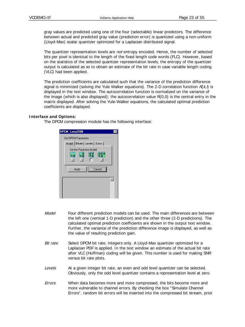
gray values are predicted using one of the four (selectable) linear predictors. The difference between actual and predicted gray value (prediction error) is quantized using a non-uniform (Lloyd-Max) scalar quantizer optimized for a Laplacian distributed signal. The quantizer representation levels are not entropy encoded. Hence, the number of selected bits per pixel is identical to the length of the fixed length code words (FLC). However, based on the statistics of the selected quantizer representation levels, the entropy of the quantizer output is calculated as so to obtain an estimate of the bit rate in case variable length coding (VLC) had been applied. The prediction coefficients are calculated such that the variance of the prediction difference signal is minimized (solving the Yule Walker equations). The 2-D correlation function R(k,l) is displayed in the text window. The autocorrelation function is normalized on the variance of the image (which is also displayed); the autocorrelation value R(0,0) is the central entry in the matrix displayed. After solving the Yule-Walker equations, the calculated optimal prediction coefficients are displayed.


The DPCM compression module has the following interface:

Model Four different prediction models can be used. The main differences are between the left one (vertical 1-D prediction) and the other three (2-D predictions). The calculated optimal prediction coefficients are shown in the output text window. Further, the variance of the prediction difference image is displayed, as well as the value of resulting prediction gain.

Bit rate Select DPCM bit rate, integers only. A Lloyd-Max quantizer optimized for a

Laplacian PDF is applied. In the text window an estimate of the actual bit rate after VLC (Huffman) coding will be given. This number is used for making SNR versus bit rate plots.

Levels At a given integer bit rate, an even and odd level quantizer can be selected.

Obviously, only the odd level quantizer contains a representation level at zero. Errors When data becomes more and more compressed, the bits become more and

more vulnerable to channel errors. By checking the box “Simulate Channel Errors”, random bit errors will be inserted into the compressed bit stream, prior


to decompression. In this way an impression can be obtained of the effects of (simple) channel errors. Different bit error probabilities can be selected, namely 0.005 (0.5% of the bits are erroneous), 0.001, 0.0005, and 0.0001.

Images Displayed:

The prediction difference or prediction error image The prediction difference inside the DPCM loop is shown. This is the data that is

fed into the quantizer. Zero values are displayed as gray, while positive and negative values are displayed as brighter or darker than the overall gray value. The prediction difference is scaled for maximum visibility.


Remark:

At low bit rates you may see funny effects in certain compressed images (in particular images with large regions of constant gray value). These oscillation patterns are not caused by a programming bug, but by particular combinations of predictor and quantizer. In fact, these degradations illustrate that because the prediction coefficients are calculated to be optimal in the absence of quantization, using them in combination with quantization may yield far from optimal results.


Vector Quantization (VQ) Compression Algorithm:

The VQ compression module implements a straightforward full search vector quantizer. Each input vector (a image subblock of user-selectable size) is compared against the codebook vectors, and the one with the smallest mean-square difference is selected as representation vector. The output of VQ, i.e., the addresses of the selected VQ codebook vectors, are not entropy encoded (i.e., FLC coded). Hence, the bit rate can be derived directly from the number of bits per codebook vector. Code books can be designed on-line using the loaded image, and subsequently saved for use with other images. The codebooks themselves are saved as image with a particular structure. See also codebook design.


The VQ compression module has the following interface:


Codebook Choose to create a new VQ codebook or load an existing codebook from disk. The other two tabs are disabled until a codebook has been designed or loaded.

Bits Select the number of bits per codebook vector. Bit rates for which no codebook

has been designed are disabled. The choice of the number of bits per codebook vector in combination with the codebook vector size, determines the bit rate of the compressed image.

Errors When data becomes more and more compressed, the bits become more and

more vulnerable to channel errors. By checking the box “Simulate Channel Errors”, random bit errors will be inserted into the compressed bit stream, prior to decompression. In this way an impression can be obtained of the effects of (simple) channel errors. Different bit error probabilities can be selected, namely 0.005 (0.5% of the bits are erroneous), 0.001, 0.0005, and 0.0001.

Images Displayed:

Codebook The codebook loaded is displayed. This codebook is stored and displayed as an

image with a particular structure. See codebook design. Decoded image The decoded image is shown.


Codebook Design for Vector Quantization Existing Codebooks:

The following dialog is opened when “Load Codebook” is pressed.


The directory opened is the one set under “HelpSettings”. The codebook names usually show the size of the codebook vectors (e.g. 4x4 blocks or 2x8 block), and the minimum and maximum rate stored in the codebook. A single codebook stores the codebook vectors for multiple bit rates. The codebooks are simply bmp images, and can also be viewed using a normal image viewer. The organization of the codebook vectors is as follows. From top to bottom, the codebooks of increasing rate are stored, sometimes in a row wrapped fashion. The following figure shows an example of a (very small) codebook with codebook vector size 4x4 pixels for bit rates of 0.0625 to 0.31 bit per pixel.

The top row first contains some numerical data about the stored codebook (in particular, the size of the codebook vectors, and the minimum and maximum number of bits per codebook vector), followed by the codebook vectors at the smallest number of bits per codebook vector (which is 1 in this case, hence 2 codebook vectors of size 4x4 pixels). Following are the codebooks for the rates 2 bit/vector (4 codebook vectors), 3 bits/vector, 4 bits/vectors and finally 5 bits/vector (32 codebook vectors).

Designing New Codebooks:

The following dialog is opened when “Create Codebook” is pressed.


The currently loaded image (start image) is considered as training image, and used to design a codebook from. In general multiple training images are necessary for robust codebooks. If you want to use multiple training images, first combine your images into a single image using a simple program like MSPaint. Then load the composite image as start image, and invoke the codebook design procedure. This codebook design menu has parameters that can be grouped into two classes:

Codebook vector parameters

Horizontal and vertical dimension of the codebook vectors can be selected independently. The dimensions must be a multiple of the image dimensions. Minimum and maximum bit rate for which the codebook needs to be designed. Note that the design of a codebook is exponentially increasing with the bit rate. The design of larger codebooks (10-12 bits) may take quite some time – of course memory and CPU-speed dependent – but be prepared to wait and get some coffee! It is generally advisable to start with smaller codebook size. The program will output some information in the text window so you will know it is still alive. Note that the design procedure can not be interrupted.

Initialization and convergence

The design of a codebook is an iterative procedure. As in any iterative procedure, the iterations must be initialized. The codebook vectors can be initialized using random numbers in the range [0,255] or with constant gray values, uniformly distributed over the codebook vectors in the range [0,255]. The results will be different and convergence speed may be different. The codebook design iterations have to be truncated after sufficient convergence. Two thresholds are in effect, namely the difference in MSE in two subsequent iterations (calculated on the current estimate of the codebook and the training vectors) which is called the convergence threshold, and the number of iterations carried out (to prevent infinite computation time). Setting smaller convergence thresholds and/or larger number of iterations yields larger computation times.

Saving codebooks Codebooks that have been designed, can be used immediately. They can also be


saved for later use, for instance in combination with another image.

Codebooks of different rates are designed sequentially, starting at the lowest rate codebook. The MSE between the current estimate of the codebook and the training vectors is shown in the text window for each iteration. Observe the decrease of this number. In the initial iterations sometimes no training vectors are assigned to codebook vectors. The percentage of no-assignments is shown in the text window. These no-assignment codebook vectors are re-initialized with constant gray values.


Fractal Coding (FRAC) Compression Algorithm:

The Fractal Image Coding module implements a variable-block based fractal coder. For each range block, a suitable mapping of a domain block is searched. A threshold determines whether a range block needs to be further split into smaller blocks (quad-tree structure). Minimum and maximum block sizes can be set. Also, the number of bits to encode each mapping can be selected.

Interface and Options: The fractal image compression module has the following interface:

Size: The maximum and minimum range block size can be set here. Generally, the

smaller the range blocks are allowed to become, the higher the bit rate and the longer the computation time for encoding and decoding.

Threshold: To determine if a range block has to be split into four smaller range blocks, a check is carried out on the MSE of the range block and the best domain block found. If the square root of the MSE (RMS) is larger than the threshold set, the range block will be split.

Bits: The domain to range block mappings are determined by a shift vector (fixed rate, dependent on range block size), an isomorphic projection (fixed 3 bits), and the scale and offset for the intensity transformation. The number of bits for


the scale and offset factor can be selected here. The more bits are chosen, the higher the bit rate of the compressed image.

Iterations: The decoder carries out an iterative reconstruction to recover the compressed image. Here the number of iterations can be chosen. Once an image is encoded, choosing a different number of iterations does not require compressing the image again. The compressed image is stored on disk as a bit stream in the file “FractalCodedImageBitStream.fif”. The decoder reads bits from this file.

Images Displayed:


Remark:

Fractal compression as implemented here does not have a possibility for rate control. Therefore, as you vary parameters both the bit rate and the MSE/SNR will change. Keep this in mind when comparing results.


Subband (Wavelet) Coding (SBC) Compression Algorithm:

The SBC compression module implements SBC coder with global (non locally adaptive) bit allocation. Different subband decompositions can be selected, and different QMF filters can be selected. Multiple subbands are obtained by tree structured subband decompositions. The subbands are quantized based on a user-selectable PDF model. The quantizer representation levels are entropy encoded.


The SBC compression module has the following interface:


Decomp: The subband decomposition structure can be selected here. A choice of 6 common decompositions is available, though many more decompositions can be envisioned. The quantization of the subbands can be switched off to measure the quality of filter banks that carry out the subband decomposition and reconstruction.

Filter: The number of filter coefficients for the low pass QMF analysis filter can be

selected. The other filters are derived from this low-pass QMF filter. The filters used are those designed by Johnston.

Subs: The quantization of the SBC coefficients can be selected. Subband 1 (low-pass

subband) can be compressed independently of the higher frequency subbands. For the subbands a choice can be made between PCM and DPCM. The quantizers

considered for each subbands depend on the selected PDF. The c-value specifies the shape parameter of a generalized Gaussian PDF. If DPCM is chosen, the DPCM prediction model can be selected. Data within a single subband are all quantized with the same quantizer. Thus the SBC compression implemented here has a global quantization behavior. In contrast to this, SPIHT, EZW, and JPEG2000 compression schemes have a local quantization behavior.

Bit rate: Different bit rates can be selected. The limited number of choices here has been

hard coded, but is not essential to SBC compression as the bit allocation procedure (implemented here as the greedy or convex hull algorithm) can achieve any desired (overall) bit rate. Normally entropy coding (Huffman) is applied to the quantizer outputs, but in order to accommodate experiments with channel bit errors, the entropy coding should be switched off.

Errors: This tab allows the injection of random bit errors into the compressed bit stream,

prior to decompression. In this way an impression can be obtained of the effects of (simple) channel errors. Different bit error rates can be selected, namely 0.005 (0.5% of the bits are erroneous), 0.001, 0.0005, and 0.0001. Bit errors can only be injected if the entropy coding of the quantizer output levels has been switched off.

Images Displayed:


The original and compressed subbands

The subbands of the image to be compressed are shown to the right of the start image. The subbands are organized according to the decomposition scheme selected. The low frequency subband is shown in the upper left corner, with increasing frequency bands to the right and below. In order to visualize the subband information, the subbands are scaled to maximum intensity range. “Gray” means zero value, and negative and positive values are darker and brighter, respectively, than the zero value. The actual variance of the subbands can be found in the text window. Because of the scaling, no direct interpretation of the importance (variance) of subband data can be derived from the displayed data.


After quantization and VLC encoding, the subbands are transmitted and decoded by the receiver. The quantized subbands are shown immediately below the original subbands. Subbands that have received zero bits in the bit allocation are entirely gray. The actual bit allocation results can be found in the text window. Again, subbands are scaled for maximum visibility. Note that this may be misleading when comparing subbands of the original and compressed images, since these may be scaled differently. The effect of channel errors is also visible in the individual subbands.

The left image shows an example of original subbands (prior to quantization),

while the right image shows subbands after quantization.


Discrete Cosine Transform (DCT) Compression Algorithm:

The DCT compression module implements a DCT coder with global (not locally adaptive) bit allocation. Different DCT block sizes can be selected. The DCT coefficients are quantized based on a user-selectable PDF model. The quantizer representation levels are entropy encoded.


The DCT compression module has the following interface:


Size: The size of the DCT transform blocks can be selected (2x2, 4x4, 8x8, 16x16). The quantization of the DCT coefficients can be switched off to measure the quality of forward and reverse DCT transform.

Coefs: The quantization of the DCT coefficients can be selected. The first DCT coefficient

(mean value in the DCT block) can be compressed independently of the higher frequency DCT coefficients.

For the DCT coefficients a choice can be made between PCM and DPCM. The

quantizers considered for each DCT coefficient depend on the selected PDF. The c-value specifies the shape parameter of a generalized Gaussian PDF. If DPCM is chosen, the DPCM prediction model can be selected. The DCT coefficients with the same index (originating from different DCT blocks) are all quantized with the same quantizer. In this way the bit allocation can optimize the allocation of the bits to all DCT coefficients. Thus the DCT compression implemented here has a global quantization behavior. In contrast to this, JPEG is a DCT compression scheme with local quantization behavior.

Bit rate: Different bit rates can be selected. The limited number of choices here has been

hard coded, but is not essential to DCT compression as the bit allocation procedure (implemented here as the greedy or convex hull algorithm) can achieve any desired (overall) bit rate. Normally entropy coding (Huffman) is applied to the quantizer outputs, but in order to accommodate experiments with channel bit errors, the entropy coding should be switched off.


prior to decompression. In this way an impression can be obtained of the effects of (simple) channel errors. Different bit error rates can be selected, namely 0.005 (0.5% of the bits are erroneous), 0.001, 0.0005, and 0.0001. Bit errors can only be injected if the entropy coding of the quantizer output levels has been switched off.

Display: The DCT coefficients obtained after transformation and after quantization can be

displayed in two ways, namely: • group by index (collections) of DCT coefficients. In this case the DCT

coefficients with the same index from all DCT blocks are collected in a single set. These sets are much like subband coefficients, and give an easy to


understand impression of the bit allocation result, • group by DCT Blocks in the correct spatial location. In this case the DCT

coefficients are shown as NxN blocks that sit in the spatial position corresponding to the NxN pixels the DCT coefficients are calculated from. For visibility purposes the DCT coefficients are scaled. This display mode gives an easy to understand impression of the local frequency content of an image, and – after the bit allocation – an impression of which part of an image is easy or hard to compress.

Images Displayed:


The original and compressed DCT coefficients

The DCT coefficients of the image to be compressed are shown to the right of the start image. The DCT coefficients are organized according to the Display mode selected. In order to visualize small DCT coefficients, the values are scaled to maximum intensity range. “Gray” means zero value, and negative and positive values are darker and brighter, respectively, than the zero value. The actual variance of the subbands can be found in the text window. Because of the scaling, no direct interpretation of the importance (variance) of DCT coefficients can be derived from the displayed data.

After quantization and VLC encoding, the DCT coefficients are transmitted and

decoded by the receiver. The quantized DCT coefficients are shown immediately below the original DCT coefficients. DCT coefficients that have received zero bits in the bit allocation are entirely gray. The actual bit allocation results can be found in the text window. Again, DCT coefficients are scaled for maximum visibility. The effect of channel errors is also visible in the individual DCT coefficients. The quantized DCT coefficients are organized depending on the Display mode selected. The left image shows an example of quantized DCT coefficients if display mode Collection is selected, while the right image shows the DCT coefficients if the option DCT Blocks is selected.



JPEG Compression Standard (JPEG) Compression Algorithm:

The JPEG compression module implements the full JPEG compression standard. Several optimization options can be selected. The module writes a jpg- file to disk (in the user-output directory), which can be viewed with any JPEG viewer.


The PCM compression module has the following interface:

Bit rate: The JPEG quality factor Q can be set here. By selecting the quality factor, the bit rate is implicitly defined, but the bit rate is not known beforehand. Instead of setting the quality factor, a bit rate can be selected. The quality setting corresponding with this bit rate will be determined by a simple search procedure. The resulting quality (Q) factor is shown in the text window.

Quant: The quantization of the DCT coefficients is carried out using the standard JPEG

quantizers, which can – however – be influenced by selecting a particular quantization or normalization matrix. The normalization matrix to be used can be selected here. The options are • the standard JPEG normalization matrix for luminance information, • the standard JPEG normalization matrix for chrominance information, • a normalization matrix filled with equal weights for all DCT coefficients

(weight=50). • a “high-emphasis” normalization matrix, that puts more emphasis on high

frequency DCT coefficients rather than on low-frequency DCT coefficients. This matrix has been added for educational purposes only, and will never be used in practice.

Notice that in JPEG both quality factor and SNR vary as one changes the selection of the normalization matrix.

The user quality factorQ and normalization matrix N(u,v) are used as follows to quantize the DCT coefficients F(u,v):


F u v NINTF u v

Q N u v*( , )

( , )' ( , )

=

where the minimal value of Q' N(u,v) is 1.0. Q' is related to the user quality factor Q as shown in the following graph:

0 10 20 30 40 50 60 70 80 90 100 0

1

2

3

4

5

6 Q'

Q

Huffman: Different entropy coding tables can be selected here, namely no entropy coding (i.e. fixed length coding) for the DCT coefficients, standard VLC, or a VLC table optimized for the image under consideration.

Smooth: If checked, the decompressed image is smoothed somewhat to suppress blocking

artifacts. Does not influence the compression, only the visual quality after decoding.

Markers: In the JPEG module, errors can be injected into the actual JPEG stream. This

means that VLC codes, header information, and other crucial information may get corrupted. To block the effect of progressively worsening VLC decoding errors, unique markers may be inserted into the JPEG bit stream. The periodicity of these markers can be selected here. Notice that as more frequently markers are inserted, the overall bit rate will go up, or – if a fixed bit rate has been set – the SNR will go down.


prior to decompression. In this way an impression can be obtained of the effects of (simple) channel errors. Different bit error rates can be selected, namely 0.005 (0.5% of the bits are erroneous), 0.001, 0.0005, and 0.0001. Bit errors potentially corrupt crucial information such as header information (image size, VLC tables). In case the errors are too severe, decoding is interrupted.

Images Displayed:

Compressed bitstream: The compressed image is written to disk in a file name

“JpegCodedImageBitStream.jpg”. This file contains the JPEG compressed data, embedded in the JFIF header protocol. The file can be viewed with any standard image display or processing application.

Decoded image


The decoded image is shown.

Viewing of DCT coefficients: The JPEG module itself does not show the (quantized) DCT coefficients. To view

these, use the option “Set as start image” on the JPEG decompressed image. Then run the DCT compression module on this image, using 8x8 DCT blocks and switching off the encoding of the DCT coefficients. The DCT coefficients computed from the JPEG compressed image will now be displayed. Both display modes (Collections and DCT Blocks) are instructive to study.


Embedded Zero-Tree Wavelets (EZW) Compression Algorithm:

The EZW compression module implements a embedded-zero tree wavelet encoder. The bit stream is continuously scalable (or progressively coded), which means that the decoder can read the first N bits to decode the image at rate N/(#rows.#columns) bit per pixel.

Interface and Options: The EZW compression module has the following interface:

Encoder bit rate The encoder bit rate can be selected. Levels Select the number of levels up to which the image will be decomposed. Decoder bit rate The coded image will be decoded until the selected decoder bit rate is

reached, the rest of the coded information will not be used to decode the image.

Images Displayed:



The original and compressed wavelet coefficients

The Windows containing the original wavelet coefficients (image subbands) and the compressed wavelet coefficients are similar as in the SBC module. The picture below shows the original (unquantized) wavelet coefficients

Remark:

The term “number of levels” is very confusing. If an image is not decomposed, what is the number of levels in this case? Zero or one? In the VcDemo we refer to “the number of resolution levels”. No splitting means one resolution level, one split means two resolution levels, etc. This terminology is used in both EZW and SPIHT.


Set-Partitioning in Hierarchical Trees (SPIHT) Compression Algorithm:

The SPIHT compression module implements a wavelet based encoder. The bit stream is continuously scalable, which means that the decoder can read the first N bits to decode the image at rate N/(#rows.#columns) bit per pixel. The SPIHT algorithm used here is based on commercial implementation of PrimaComp Inc. Troy, NY, USA.

Interface and Options: The SPIHT compression module has the following interface:

Encoder bit rate A bit rate can be selected here to which to current image will be encoded.

The coded file will be at the selected bit rate. Smoothing Seven levels of smoothing can be selecting. This will adjust the filter

coefficients to get a smoothing effect ( 0 is no smoothing, 7 is smoothing


level 7.) Decoder bit rate The coded image will be decoded until the selected decoder bit rate is

reached, the rest of the coded information will not be used to restore the image. The decoder bit rate MUST be smaller than the encoded bit rate. Note that the decoder bit rates is not automatically adjusted for changing encoder bit rate.

The number of splits (see “Remark”) is determined by the SPIHT algorithm itself and is not a selectable parameter here. If you want to play with this parameter, use the SBC or EZW module instead as the overall effects are more or less the same as in SPIHT.

Many of the reported compression factors in VcDemo are calculated on the basis of VLC assignments, but without actually creating the compressed file. The SPIHT encoder does create a temporary file on disk and the decoder reads this file. For that reason the reported compression factors and bit rate in the SPIHT module are exact.

Images Displayed: Decoded image The decoded image is shown. The original and compressed wavelet coefficients

The Windows containing the original wavelet coefficients (image subbands) and the compressed wavelet coefficients are similar as in the SBC module. The picture below shows the original (unquantized) wavelet coefficients

Remark:

The term “number of levels” is very confusing. If an image is not decomposed, what is the number of levels in this case? Zero or one? In the VcDemo we refer to “the number of resolution levels”. No splitting means one resolution level, one split means two resolution levels, etc. This terminology is used in both EZW and SPIHT.



JPEG-2000 Image Compression Standard (JPEG2000) Compression Algorithm:

The JPEG2000 compression module implements the JPEG2000 image compression standard. The implementation is based on JPEG2000 verification model 7.1. The bit stream is continuously scalable, which means that the decoder can read the first N bits to decode the image at rate N/(#rows.#columns) bit per pixel.

Interface and Options: The JPEG2000 compression module has the following interface:

Encode: The encoder bit rate can be selected. Depending on the selected encoding bit

rate, a range of decoding bit rates becomes available. Quant: Several parameters can be set that determine the quantization of the wavelet

coefficients: • Lossless quantization. In this case the decoded image is nearly

identical to the original (except for rounding errors). The encoding/decoding bit rate cannot be controlled.

• SNR layering: The compressed data is organized such that the bits (i.e. wavelet coefficient/bit planes) that contribute most to the quality of the image (expressed in SNR) are included first in the bit stream. Therefore, truncating the stream will give a larger SNR than without SNR layering.

• Code block: The size of the block in the wavelet domain for which parameters are set. Smaller blocks allow for better adaptation to local content at the price of a larger overhead.

Levels: Several parameters can be set that determine the wavelet decomposition:

• Number of resolution levels determines how often the low frequency band of wavelet coefficients is split.

• Perfect reconstruction filter bank: The filter bank is perfectly reconstructing, avoiding compression differences due to the wavelet decomposition and reconstruction process.

Decode: The decoder bit rate can be selected. Depending on the selected encoding bit

rate, a range of decoding bit rates is available.


VisMask: A parameterized visual masking function can be selected, which influenced the

quantization process. Tiling: The encoding process can be carried out on image tiles. This allows for partial

decoding of image tiles image, independent of other tiles.

Images Displayed: Decoded image The decoded image is shown. Output in text window

The target file size (determined by the selected encoding bit rate) and the attained file size are given. Dependent on the decoding bit rate, a certain number of bits are decoded, yielding a certain MSE and (P)SNR.

Remark: The encoding process has a lot of options, which are sometimes dependent on each other. For that reason, when changing one parameter value other parameters may also change automagically.


Motion Estimation (ME) Compression Algorithm:

The Motion Estimation module implements several block-based motion estimators. The simplest motion estimator is the full search block matcher. Parameters such as the block size and the search window (maximum displacement) can be set. Advanced options of the motion estimators include more efficient search patterns (One-at-a-time, N-Step) and hierarchical block matching. The motion estimation and compensation results are visualized as moving video clips. Motion is estimated on all frames of the image sequences. The estimation process can be interrupted by pressing any key.


The motion estimation module has the following interface:


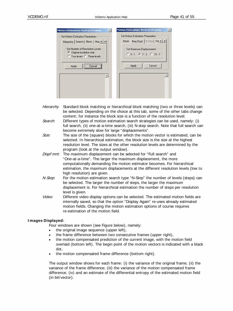
Hierarchy Standard block matching or hierarchical block matching (two or three levels) can be selected. Depending on the choice at this tab, some of the other tabs change content; for instance the block size is a function of the resolution level.

Search: Different types of motion estimation search strategies can be used, namely: (i) full search, (ii) one-at-a-time search, (iii) N-step search. Note that full search can become extremely slow for large “displacements”.

Size: The size of the (square) blocks for which the motion vector is estimated, can be selected. In hierarchical estimation, the block size is the size at the highest resolution level. The sizes at the other resolution levels are determined by the program (look at the output window).

Displ’mnt: The maximum displacement can be selected for “Full search” and “One-at-a-time”. The larger the maximum displacement, the more computationally demanding the motion estimator becomes. For hierarchical estimation, the maximum displacements at the different resolution levels (low to high resolution) are given.

N-Step: For the motion estimation search type “N-Step” the number of levels (steps) can be selected. The larger the number of steps, the larger the maximum displacement is. For hierarchical estimation the number of steps per resolution level is given.

Video: Different video display options can be selected. The estimated motion fields are internally saved, so that the option “Display Again” re-uses already estimated motion fields. Changing the motion estimation options of course requires re-estimation of the motion field.

Images Displayed: Four windows are shown (see Figure below), namely:

• the original image sequence (upper left), • the frame difference between two consecutive frames (upper right), • the motion compensated prediction of the current image, with the motion field

overlaid (bottom left). The begin point of the motion vectors is indicated with a black dot,

• the motion compensated frame difference (bottom right). The output window shows for each frame: (i) the variance of the original frame; (ii) the

variance of the frame difference; (iii) the variance of the motion compensated frame difference; (iv) and an estimate of the differential entropy of the estimated motion field (in bit/vector).


For the differential entropy, a simple 1-D lossless DPCM is carried out on the motion vector field horizontal and vertical components separately. Then the histograms of the DPCM differences are calculated. From the histograms the entropy of the vector field is estimated as the sum of the estimated entropy of the horizontal and vertical component.

Remark: The motion estimation module has a lot of parameters if hierarchical motion estimation is selected. It is not easy to find the optimal setting for all cases. We recommend that you initially stick to the non-hierarchical version. The fact that the parameter choice (of hierarchical motion estimation) is not easy of course also says something about design challenges in real applications of motion estimation.


MPEG Video Encoder (MEnc) Compression Algorithm:

The MPEG compression module implements an MPEG-1 and MPEG-2 encoder. The encoder produces a valid MPEG video bit stream, i.e. without a system layer. The MPEG encoder is far from optimized in bit rate-SNR and speed performance, and should only be used for studying the effects of typical MPEG parameters such as GOP, bit rate, and motion estimation.


An MPEG encoder has many different parameters that one can set. In the VcDemo, MPEG encoder the choice have been limited severely in order to for novices to get meaningful results. Therefore, the MPEG encoder works properly, but for competitive implementations control over many more parameters should be exercised.


When opening the MPEG encoder interface, all options have been deactivated until a name has been selected for the compressed MPEG file. Depending on the type of MPEG compression (MPEG-1 or MPEG-2 on the first tab) certain option are activated or deactivated. The MPEG compression module has the following interface:

File: Set the MPEG file name, and select the MPEG type (MPEG-1 or MPEG-2). Rate: Set bit rate of the compressed file, in Mbit/second. GOP: Different group of picture structures can be selected here. Although GOPs

come in a wide variety of choices, here only several standard (and non adaptive) ones have been provided for the sake of simplicity.

Motion: The maximum displacement can be selected here. The encoder uses

hierarchical motion estimation for frame-based compression, and full search for field-based compression.

Format: For MPEG-2 compressed format, the format of the video sequence can be set

here. If interlaced format is selected, the position of the first field must be indicated.

Field/Frame: In case the input video sequence has an interlaced format, the full power of

MPEG-2 can be used. There are several ways the encoder can be forced to certain option. Here, the encoder can be forced to always use frame-based motion estimation and DCT in case frame coding is used.

Images Displayed:


The encoder display the image just encoded. Since the encoder does not always process the frames time sequentially, you will see funny motion effects (movie going back and forth).

The most useful information can be found in the text window. You will find the bit rate per frame, the way the frame has been encoded (I/P/B), and the way the individual macroblocks have been compressed.

This is the legend for the first character: S: skipped I: intra coded 0: forward predicted without motion compensation F: forward frame/16x8 prediction (in frame/field pictures resp.) f: forward field prediction p: dual prime prediction B: backward frame/16x8 prediction b: backward field prediction D: frame/16x8 interpolation d: field interpolation


Second character:

space: coded, no quantizer change Q: coded, quantizer change

Remark on compatibility issues

The MPEG encoder produces an MPEG video stream. This video stream is a perfectly MPEG compliant stream, but in case you try to play it with the Windows Media player it will not work. Why? Simply because there is no system information, most notably timing information, which the media player requires. It is easily verified that with other MPEG decoders one can view the MPEG files produced by VcDemo. Alternatively, you can use the VcDemo MPEG 1/2 decoder to view the result. The MPEG decoder will play any MPEG video stream, with or without timing information and with or without system stream information.


MPEG Video Decoder (MDec) Decompression Algorithm:

The MPEG decompression module implements an MPEG-1 and MPEG-2 decoder. The decoder operates on valid MPEG video and system bit stream. Streams obtained from the Internet can be decoded by the module, but the decoder will only show the video component (no audio and timing information).


The MPEG decompression options are shown below. There are five tabs with the following parameters:

Operation: The decoder operation and output can be chosen, namely: (i) normal output, showing the decoder frames as would be shown by

any decoder; (ii) the predicted frames without adding the quantized prediction

difference that are sent from encoder to decoder in the bit stream. In this way an impression can be obtained of the prediction quality.


Notice that prediction differences will accumulate in this case; (iii) the coded prediction differences, i.e. the information sent from

encoder to decoder in the bit stream. In this way the prediction quality and the number of intra-coded macroblocks can easily be evaluated.

Display: Three display options can be switched on/off, namely:

(i) color or black-and-white display, (ii) show the motion vectors in overlay with the frame information; (iii) skip the B-frames (for slow machines, gives better motion rendering).

Video: Different video display options can be selected. The frame-by-frame option allows for evaluating individually decoded frames.

Wireless: Open the interface of the wireless channel simulator, that can inject realistic

bit/packet errors into the MPEG bit stream before MPEG decoding. Save As: The decoded MPEG stream can also be saved as a raw YUV file (plus header). Be

aware of the data expansion that you will get, and have enough disk space available if you decoded a long MPEG stream!

Images Displayed: One windows is shown containing the decoder frame, the predicted frame, or the prediction difference depending on the selected Operation choice. The text pane displays information decoded from the Mpeg stream about video format and coding parameters. During the decoding also the GOP structure is displayed. Notice that the decoding order and display order may be different in Mpeg due to the B-frames.

The overlaid motion field show the begin point of the motion vectors as a red dot. Macroblocks that have only a dot have a motion vector of zero, or have been intra-coded. By looking at the coded frame differences these two cases can be differentiated. The motion vectors shown are always backward motion vectors (as in P frames) unless a macroblock in a B frame has been predicted in a forward manner. In this case the forward motion vector is used. Some macroblocks use multiple motion vectors (B-macroblocks and in various MPEG-2 coding modes). Notice that still only one vector is shown.



Insertion of Channel Errors into MPEG Bit Stream Channel Simulation Algorithm:

The protocol/channel simulator can be activated from MPEG decoder, and operates on the MPEG bit stream opened. Effectively, the protocol/channel simulator implements part of the OSI model application layer, the transport layer, the network layer, data link layer, and the physical layer. At the OSI application layer we not only find the compression/decompression algorithms, which are of course not simulated by the wireless channel module, but also the packetization of the MPEG video stream. Either the stream is chopped into packets of 1500 bytes, or the packets are formed by aligning MPEG start codes with the packet boundaries. In the latter case the data payload has a variable length up to 1500 bytes, and an 12 byte RTP header is added to the data. At the transport layer, the UDP protocol is simulated by appropriately adding the header and checksum information (8 bytes). Finally, at the network layer 20 bytes are added to simulate the representation of IP information. At the data link layer, two medium access (MAC) protocol are simulated, namely HiperLAN(~ IEEE 802.11 like) and GPRS. In the case of HiperLAN, the number of users accessing the


channel can be selected assuming an total rate of 20 Mbit/sec. The overall bit rate offered to the channel is equal to the number of users multiplied by the bit rate of the MPEG bit stream opened. If the overall bandwidth is larger than 20 Mbit/sec (too many users), the contention mechanism will cause packets to be dropped, yielding decoding errors. For GPRS, four modulation/error protection modes can be selected (CS-1 to CD-4). If the GPRS transmission bandwidth is less than the bit rate of the MPEG bit stream opened, the transmission of the video file will be less-than-real time, but in the wireless channel simulator this will not cause packets to be dropped. Finally, at the physical layer, two different channel models can be selected namely a random bit error channel, and a burst error channel simulated through a Gilbert-Elliot Model. Note that the MPEG decoder is not very robust against bit errors (unlike the JPEG decoder implementation). For that reason, some bit error patterns may cause the decoder – and thus VcDemo – to crash. Be careful in decoding MPEG bit streams that contain bit errors/packet losses.


The Wireless Channel Simulator interface and option are shown below.

Protocol: Select the data link protocol, namely HiperLAN or GPRS RTP/Startcode alignment: If selected, the RTP overhead is added to the data, and the MPEG bit stream is

segmented such that MPEG start codes are aligned with the beginning of data packets. If this option is not selected, the MPEG stream will be chopped into packets of fixed length (1500 bytes).

Number of users (HiperLAN): The number of other users on the same channel can be selected. All users

together should fit in 20 Mbit/sec. In case the overall bit rate, defined as the number of users multiplied by the bit rate of the MPEG stream being processed,


plus protocol overhead, approaches or surpasses 20 Mbit/sec, the contention mechanism will start to drop data packets, causing errors in the received bit stream.

Coding scheme (GPRS): One of the four GPRS coding schemes can be selected: CS-1: 25 kbit/sec, CS-2:

60 kbit/sec, CS-3: 80 kbit/sec, or CS-4: 150 kbit/sec. The higher the bit rate, the weaker are the error correcting codes.

Channel model: A random bit error channel or the Gilbert-Elliot (two state or burst error) channel

can be selected. Bit error rate: The bit error rate for the random bit error channel or the two bit error rates for

the good and bad state of the Gilbert-Elliot channel, respectively, can be set. Transition probabilities: The transition probabilities between the two states of the Gilbert-Elliot channel

can be set.

Output Data: When pressing “apply”, the MPEG compressed bit stream is passed through the protocol and channel simulator. The resulting (corrupted) MPEG file is saved on disk. Subsequently, this file can be selected for decoding (press “Decode Stream”), which returns you to the MPEG decoder with the corrupted bit stream selected for decoding. Alternatively, the channel simulator can be run again (on the original MPEG bit stream), or the operation can be canceled, returning to the decoding of the original MPEG bit stream. The text window gives information about the effects of the protocol/channel simulator, such as number of bits and packets processed, the number of bit and packet errors (uncorrectable and undetectable), and the number of packets lost due to contention with other users.


H.264 Video Encoder (HEnc) Compression Algorithm:

The H.264 video compression module implements one of the intermediate H.264 versions (test model JM 6.1). The block diagram of the H.264 motion-compensated video compression algorithm is shown below.


In comparison to earlier compression standards such as MPEG, H.264 has a number of compression options that the encoder may consider for usage, such as:

• Spatial prediction of intra-encoded 4x4 subblocks (see figure below) or 16x16 macroblocks. Different spatial predictors (especially the spatial direction of prediction) can be selected;

• Partitioning of 16x16 macroblocks into 16x8, 8x16 or 8x8 sub macroblocks, which can

be subdivided into 8x4, 4x8 or 4x4 subsubmacroblocks. Different motion vectors and temporal prediction directions can be used for the (sub)submacroblocks. Per macroblock one (for a 16x16 macroblock) up to 16 (for 16 4x4 subsubblocks) motion vectors may be used.


Motion vectors have ¼ pixel accuracy. The motion vectors themselves are predictively encoded using the median of motion vectors of three neighboring blocks, namely, left, above, and above-right of the current block (see example below).

• The basis of the decorrelating transform is a separable orthogonal transform on 4x4 blocks. The “DC coefficients” of 16 4x4 blocks in a macroblock may be decorrelated again using the same orthogonal transform. Other block sizes for the transform may also be used, e.g., 8x4 pixels. The basic4 point decorrelating transform from which all transforms are build up, is given by:

−−−−

−−=

112121112111

1121

tT

Quantization of (weighted) transform coefficients is done by a 51-step uniform quantizer.

• Entropy encoding of zig-zag scanned transform coefficients can be done using

universal VLC codes, or the more advanced CABAC coder (Context-Based Adaptive Binary Arithmetic Coding).

• A deblocking (low-pass) filter is included in the motion-compensated prediction loop

to suppress the feedback of motion compensation artifacts into future motion-compensated predictions.


The H.264 video compression module has the following interface:

File: Set the file name of the H.264 bit stream. The encoded image sequence will


be saved on disk using this file name. Intraframe: Select the options for intra-encoded frames:

• Sets the period of intra-encoded frames, i.e. how often a frames should be encoded as intra among all the non-skipped frames. IF the period is set to “0”, only the first frame of the sequence is intra-encoded.

• Quantization coarseness, specified as QP. The larger QP is, the coarser the quantization will be, hence the lower the produced number of bits per frame. The value of QP is fixed for all frames (i.e., no rate control), but the QP for the first (intra-encoded) frame can be set differently.

Intrafrm cnt: Set two additional options for encoding of intraframes, namely:

• Should 4x4 Hadamard transform be used, or only sum of absolute transform differences in 1/3 pixel search?

• Should inter pixels be used for Intra macroblock prediction? Interframe: Select the options for inter-encoded frames:

• Reference refers to the number of reference frames considered for motion estimation/compensation.

• Number of frames to be skipped between I/P encoded frames. Skipped frames can be absent from the coded bit stream, or can be encoded as B-frames dependent on the “B-frame” selection.

• Number of macroblocks to be forced-intra encoded. The forced intra encoded macroblock as randomly selected from the frame.

Intersearch: Set the maximum motion vector length for 16x16 blocks. For 8x8 and 4x4

blocks, the maximum range is half of the value selected here.

Int. srch mod: Select particular block sizes for which motion estimation/compensation is considered.

B-frames: Select the options for B-encoded frames:

• Number of B frames between two I/P encoded (non-skipped) frames. This number must be equal to or smaller than the selected number of frames to be skipped.

• Selection of the quantization coarseness. • Selection direct mode to use, spatial or temporal.

Entropy: The entropy coding technique can be selected, namely universal VLS or

CABAC.

Results shown

The text window shows a lot of information about the encoding process. In addition to the “self-explaining” ones, the output shows:

Display Order: Position of the encoded frame in display order Bit Stream Order: Position of the encoded frame in the bit stream Bit Rate: Number of bits used to encode the frame SNR: Signal to noise ratio, for the Y, U, and V component Intra MB: Number of forced intra-encoded macroblocks Sequence type: The order of I, B, and P frames. Also the quantization parameter


setting for each frame type is given SNR: The average SNR of all the encoded frames (given for Y, U, and V

frames separately) Total bits: The total number of bits for encoding the sequence, and for each

of the frame types Bit [email protected] Hz: The average bit rate (kbit/sec) and the encoded frame rate. Mode used: For each frame type, and each mode, the number of time a mode

has been selected Motion info bits: The number of bits used for motion information Bit usage: The number of bits used for each frame type, divided into

categories. Average bits/frm: The average number of bits per frame used for each frame type.

Remark:

The implementation is based on H.264 Test Model JM 6.1. The resulting bit stream is nearly compliant to H.264 standard, but not quite the same. In terms of functionality and quality, the differences are negligible. However, the bit stream produced is most likely not decodable by other H.264 decoders.


H.264 Video Decoder (HDec) Compression Algorithm:

The H.264 video decompression module not only decodes H.264 streams (version JM 6.1), but can also visualize the different coding decisions that the encoder has made. This includes display of the motion vectors, block partitioning, intra-coding predictions, and the costs (in number of bits) per encoded macroblock. The decoder operation is illustrated in the block diagram below.


The H.264 video decompression module has the following interface:


Decoder step: The entire bit stream can be decoded (all frames at once), or the decoder can go frame by frame.

Input stream: Display the macroblock information as encoded in the bit stream.

Intra-encoded macroblocks can be clearly identified as these contain color information. Of the inter-encoded macroblocks only the luminance information is shown. These blocks often seem uniformly gray (because the amplitudes are small), but looking at the data closely will reveal certain structures.

Motion vectors: Display the motion vectors as encoded in the bit stream. Both forward

(purple) and backward (blue) motion vectors are shown (see displayed legend). The motion vector field can be displayed with or without the decoded picture in the background.

Intra prediction: Displays the intra prediction modes, i.e. the direction in which a block has

been intra-predicted. A dot indicates mode 2 (DC mode). Selecting this option together with the option “Motion vectors” will show the coding decisions for all blocks in the frame (see example below). The intra-prediction direction vectors are colored yellow.

Block division: Displays the partitioning and coding decisions per macroblock. The

following colors are used (see also displayed legend): • Green : P-macroblocks • Purple : Direct-macroblocks (direct copy of other

macroblock) • Blue : B-macroblocks • Yellow : I-macroblocks

MB bits usage: The costs of each macroblock in terms of the number of bits can be

displayed as gray value. These costs can be shown separately, or can be shown in overlay with the motion vectors or macroblock partitioning.

Save: The decoded H.264 bit stream can be saved as a raw YUV file. This file

can be displayed by VcDemo’s video play option. Images Displayed:


In addition to the decoded image sequence, information can be displayed about decision the encoder made. Depending on the options selected, one to 5 windows (plus a legend window) will be shown, containing:

• The decoded sequence, • The information in the input stream (encoded transform coefficients), • The bit costs per macroblock (with or without being overlaid by the motion field or

macroblock partitioning), • The motion and/or intra-prediction vectors, • The macroblock partitioning and coding decisions.

The following two figures illustrate what the latter windows could look like.

Results shown: The text window shows a lot of information extracted from the H.264 bit stream.

Display Order: Position of the encoded frame in display order Bit Stream Order: Position of the encoded frame in the bit stream Picture Type: Coding type of picture (I, P, B, etc) Mode Usage: Number of times a particular encoding mode is used

Remark:

The decoder implementation is based on H.264 Test Model JM 6.1. Different test model releases (and H.264 draft standards) may have slightly different bit stream syntax. The decoder will decompress H.264 bit streams produced by VcDemo, but can most likely not decode bit streams produced by other H.264 decoders.


Documents

VcDemo Application Help - Inriapeople.rennes.inria.fr/Aline.Roumy/teaching/VCDEMO.pdf · VCDEMO.rtf VcDemo Application Help Page 2 of 55 . ... The Image and Video Compression Learning