Variations on Memetic Algorithmsfor Graph Coloring Problems

Laurent Moalic∗1 and Alexandre Gondran†2

1Univ. Bourgogne Franche-Comté, UTBM, OPERA, Belfort, France2ENAC, French Civil Aviation University, Toulouse, France

Abstract - Graph vertex coloring with a given number ofcolors is a well-known and much-studied NP-complete prob-lem. The most effective methods to solve this problem areproved to be hybrid algorithms such as memetic algorithmsor quantum annealing. Those hybrid algorithms use a pow-erful local search inside a population-based algorithm. Thispaper presents a new memetic algorithm based on one ofthe most effective algorithms: the Hybrid Evolutionary Al-gorithm (HEA) from Galinier and Hao (1999). The pro-posed algorithm, denoted HEAD - for HEA in Duet - workswith a population of only two individuals. Moreover, a newway of managing diversity is brought by HEAD. These twomain differences greatly improve the results, both in termsof solution quality and computational time. HEAD has pro-duced several good results for the popular DIMACS bench-mark graphs, such as 222-colorings for <dsjc1000.9>, 81-colorings for <flat1000_76_0> and even 47-colorings for<dsjc500.5> and 82-colorings for <dsjc1000.5>.

Keywords - Combinatorial optimization, Metaheuristics,Coloring, Graph, Evolutionary

1 IntroductionGiven an undirected graphG = (V,E) with V a set of verticesand E a set of edges, graph vertex coloring involves assigningeach vertex with a color so that two adjacent vertices (linked byan edge) feature different colors. The Graph Vertex ColoringProblem (GVCP) consists in finding the minimum number ofcolors, called chromatic number χ(G), required to color thegraph G while respecting these binary constraints. The GVCPis a well-documented and much-studied problem because thissimple formalization can be applied to various issues such asfrequency assignment problems [1, 2], scheduling problems [3,4, 5] and flight level allocation problems [6, 7]. Most problemsthat involve sharing a rare resource (colors) between differentoperators (vertices) can be modeled as a GVCP. The GVCP isNP-hard [8].

Given k a positive integer corresponding to the number ofcolors, a k-coloring of a given graph G is a function c thatassigns to each vertex an integer between 1 and k as follows :

c : V → {1, 2..., k}v 7→ c(v)

∗laurent.moalic@utbm.fr†alexandre.gondran@enac.fr

The value c(v) is called the color of vertex v. The verticesassigned to the same color i ∈ {1, 2..., k} define a color class,denoted Vi. An equivalent view is to consider a k-coloring asa partition of G into k subsets of vertices: c ≡ {V1, ..., Vk}.

We recall some definitions :

• a k-coloring is called legal or proper k-coloring if itrespects the following binary constraints : ∀(u, v) ∈E, c(u) 6= c(v). Otherwise the k-coloring is callednon legal or non proper; and edges (u, v) ∈ E such asc(u) = c(v) are called conflicting edges, and u and vconflicting vertices.

• A k-coloring is a complete coloring because a color isassigned to all vertices; if some vertices can remain un-colored, the coloring is said to be partial.

• An independent set or a stable set is a set of vertices, notwo of which are adjacent. It is possible to assign thesame color to all the vertices of an independent set with-out producing any conflicting edge. The problem of find-ing a minimal graph partition of independent sets is thenequivalent to the GVCP.

The k-coloring problem - finding a proper k-coloring of agiven graph G - is NP-complete [9] for k > 2. The bestperforming exact algorithms are generally not able to find aproper k-coloring in reasonable time when the number of ver-tices is greater than 100 for random graphs [10, 11, 12]. Onlyfor few bigger graphs, exact approaches can be applied suc-cessfully [13]. In the general case, for large graphs, one usesheuristics that partially explore the search-space to occasion-ally find a proper k-coloring in a reasonable time frame. How-ever, this partial search does not guarantee that a better solutiondoes not exist. Heuristics find only an upper bound of χ(G) bysuccessively solving the k-coloring problem with decreasingvalues of k.

This paper proposes two versions of a hybrid metaheuris-tic algorithm, denoted HEAD’ and HEAD, integrating a tabusearch procedure with an evolutionary algorithm for the k-coloring problem. This algorithm is built on the well-known Hybrid Evolutionary Algorithm (HEA) of Galinier andHao [14]. However, HEAD is characterized by two originalaspects: the use of a population of only two individuals andan innovative way to manage the diversity. This new simpleapproach of memetic algorithms provides excellent results onDIMACS benchmark graphs.

1

arX

iv:1

401.

2184

v2 [

cs.A

I] 1

7 D

ec 2

016

The organization of this paper is as follows. First, Section 2reviews related works and methods of the literature proposedfor graph coloring and focuses on some heuristics reused inHEAD. Section 3 describes our memetic algorithm, HEADsolving the graph k-coloring problem. The experimental re-sults are presented in Section 4. Section 5 analyzes why HEADobtains significantly better results than HEA and investigatessome of the impacts of diversification. Finally, we considerthe conclusions of this study and discuss possible future re-searches in Section 6.

2 Related worksComprehensive surveys on the GVCP can be found in [15, 16,17]. These first two studies classify heuristics according tothe chosen search-space. The Variable Space Search of [18]is innovative and didactic because it works with three differentsearch-spaces. Another more classical mean of classifying thedifferent methods is to consider how these methods explore thesearch-space; three types of heuristics are defined: constructivemethods, local searches and population-based approaches.

We recall some important mechanisms of TabuCol and HEAalgorithms because our algorithm HEAD shares common fea-tures with these algorithms. Moreover, we briefly present someaspects of the new Quantum Annealing algorithm for graphcoloring denoted QA-col [19, 20, 21] which has produced,since 2012, most of the best known colorings on DIMACSbenchmark.

2.1 TabuColIn 1987, Hertz and de Werra [22] presented the TabuCol algo-rithm, one year after Fred Glover introduced the tabu search.This algorithm, which solves k-coloring problems, was en-hanced in 1999 by [14] and in 2008 by [18]. The three basicfeatures of this local search algorithm are as follows:

• Search-Space and Objective Function: the algorithm isa k-fixed penalty strategy. This means that the numberof colors is fixed and non-proper colorings are taken intoaccount. The aim is to find a coloring that minimizes thenumber of conflicting edges under the constraints of thenumber of given colors and of completed coloring (see[16] for more details on the different strategies used ingraph coloring).

• Neighborhood: a k-coloring solution is a neighbor of an-other k-coloring solution if the color of only one con-flicting vertex is different. This move is called a critic1-move. A 1-move is characterized by an integer couple(v, c) where v ∈ {1, ..., |V |} is the vertex number andc ∈ {1, ..., k} the new color of v. Therefore the neighbor-hood size depends on the number of conflicting vertices.

• Move Strategy: the move strategy is the standard tabusearch strategy. Even if the objective function is worse,at each iteration, one of the best neighbors which are notinside the tabu list is chosen. Note that all the neighbor-hood is explored. If there are several best moves, onechooses one of them at random. The tabu list is not the

list of each already-visited solution because this is com-putationally expensive. It is more efficient to place onlythe reverse moves inside the tabu list. Indeed, the aim is toprevent returning to previous solutions, and it is possibleto reach this goal by forbidding the reverse moves duringa given number of iterations (i.e. the tabu tenure). Thetabu tenure is dynamic: it depends on the neighborhoodsize. A basic aspiration criterion is also implemented: itaccepts a tabu move to a k-coloring, which has a betterobjective function than the best k-coloring encounteredso far.

Data structures have a major impact on algorithm efficiency,constituting one of the main differences between the Hertz andde Werra version of TabuCol [22] and the Galinier and Haoversion [14]. Checking that a 1-move is tabu or not and up-dating the tabu list are operations performed in constant time.TabuCol also uses an incremental evaluation [23]: the objec-tive function of the neighbors is not computed from scratch,but only the difference between the two solutions is computed.This is a very important feature for local search efficiency.Finding the best 1-move corresponds to find the maximumvalue of a |V | × k integer matrix. An efficient implementa-tion of incremental data structures is well explained in [15].

Another benefit of this version of TabuCol is that it has onlytwo parameters, L and λ to adjust in order to control the tabutenure, d, by:

d = L+ λF (s)

where F (s) is the number of conflicting vertices in the curentsolution s. Moreover, [14] has demonstrated on a very largenumber of instances that with the same setting (L a randominteger inside [0; 9] and λ = 0.6), TabuCol obtained verygood k-colorings. Indeed, one of the main disadvantages ofheuristics is that the number of parameters to set is high anddifficult to adjust. This version of TabuCol is very robust. Thuswe retained the setting of [14] in all our tests.

2.2 Memetic Algorithms for graph coloring andHEA

Memetic Algorithms [24] (MA) are hybrid metaheuristics us-ing a local search algorithm inside a population-based algo-rithm. They can also be viewed as specific Evolutionary Algo-rithms (EAs) where all individuals of the population are localminimums (of a specific neighborhood). In MA, the mutationof the EA is replaced by a local search algorithm. It is very im-portant to note that most of the running time of a MA is spent inthe local search. These hybridizations combine the benefits ofpopulation-based methods, which are better for diversificationby means of a crossover operator, and local search methods,which are better for intensification.

In graph coloring, the Hybrid Evolutionary Algorithm(HEA) of Galinier and Hao [14] is a MA; the mutation ofthe EA is replaced by the tabu search TabuCol. HEA is oneof the best algorithms for solving the GVCP; From 1999 un-til 2012, it provided most of the best results for DIMACSbenchmark graphs [25], particularly for difficult graphs suchas <dsjc500.5> and <dsjc1000.5> (see table 1). Theseresults were obtained with a population of 10 individuals.

2

Figure 1: An example of GPX crossover for a graph of 10vertices (A, B, C, D, E, F, G, H, I and J) and three colors (red,blue and green). This example comes from [14].

The crossover used in HEA is called the Greedy PartitionCrossover (GPX). The two main principles of GPX are: 1)a coloring is a partition of vertices into color classes and notan assignment of colors to vertices, and 2) large color classesshould be transmitted to the child. Figure 1 gives an exampleof GPX for a problem with three colors (red, blue and green)and 10 vertices (A, B, C, D, E, F, G, H, I and J). The first step isto transmit to the child the largest color class of the first parent.If there are several largest color classes, one of them is chosenat random. After having withdrawn those vertices in the sec-ond parent, one proceeds to step 2 where one transmits to thechild the largest color class of the second parent. This processis repeated until all the colors are used. There are most prob-ably still some uncolored vertices in the child solution. Thefinal step (step k + 1) is to randomly add those vertices to thecolor classes. Notice that GPX is asymmetrical: the order ofthe parents is important; starting the crossover with parent 1or parent 2 can produce very different offsprings. Notice alsothat GPX is a random crossover: applying GPX twice with thesame parents does not produce the same offspring. The finalstep is very important because it produces many conflicts. In-deed if the two parents have very different structures (in termsof color classes), then a large number of vertices remain uncol-ored at step k + 1, and there are many conflicting edges in theoffspring (cf. figure 4). We investigate some modifications ofGPX in section 5.

2.3 QA-col: Quantum Annealing for graph col-oring

In 2012 Olawale Titiloye and Alan Crispin [19, 20, 21] pro-posed a Quantum Annealing algorithm for graph coloring, de-noted QA-col. QA-col produces most of the best-known col-orings for the DIMACS benchmark. In order to achieve thislevel of performance, QA-col is based on parallel computing.We briefly present some aspects of this new type of algorithm.

In a standard Simulating Annealing algorithm (SA), the

probability of accepting a candidate solution is managedthrough a temperature criterion. The value of the tempera-ture decreases during the SA iterations. As MA, a QuantumAnnealing (QA) is a population-based algorithm, but it doesnot perform crossovers and the local search is an SA. Theonly interaction between the individuals of the population oc-curs through a specific local attraction-repulsion process. TheSA used in QA-col algorithm is a k-fixed penalty strategy likeTabuCol: the individuals are non-proper k-colorings. The ob-jective function of each SA minimizes a linear combination ofthe number of conflicting edges and a given population diver-sity criterion as detailed later. The neighborhood used is de-fined by critic 1-moves like TabuCol. More precisely, in QA-col, the k-colorings of the population are arbitrarily orderedin a ring topology: each k-coloring has two neighbors associ-ated with it. The second term of the objective function (calledHamiltonian cf. equation (1) of [19]) can be seen as a diversitycriterion based on a specific distance applicable to partitions.Given two k-colorings (i.e. partitions) ci and cj , the distance,which we called pairwise partition distance, between ci and cjis the following :

dP (ci, cj) =∑

(u,v)∈V 2, u 6=v

[ci(u) = ci(v)]⊕ [cj(u) = cj(v)]

where ⊕ is the XOR operation and [ ] is Iverson bracket:[ci(u) = ci(v)] = 1 if ci(u) = ci(v) is true and equals 0 oth-erwise. Then, given one k-coloring ci of the population, thediversity criterion D(ci) is defined as the sum of the pairwisepartition distances between ci and its two neighbors ci+1 andci−1 in the ring topology : D(ci) = dP (ci, ci−1)+dP (ci, ci+1)which ranges from 0 to 2n(n − 1); The value of this diver-sity is integrated into the objective function of each SA. Aswith the temperature, if the distance increases, there will be ahigher probability that the solution will be accepted (attractiveprocess). If the distance decreases, then there will be a lowerprobability that the solution will be accepted (repulsive pro-cess). Therefore in QA-col the only interaction between thek-colorings of the population is realized through this distanceprocess.

Although previous approaches are very efficient the reasonsfor this are difficult to assess. They use many parameters andseveral intensification and diversification operators and thusthe benefit of each item is not easily evaluated. Our approachhas been to identify which elements of HEA are the most sig-nificant in order to define a more efficient algorithm.

3 HEAD: Hybrid Evolutionary Algo-rithm in Duet

The basic components of HEA are the TabuCol algorithm,which is a very powerful local search for intensification, andthe GPX crossover, which adds some diversity. The intensi-fication/diversification balance is difficult to achieve. In or-der to simplify the numerous parameters involved in EAs, wehave chosen to consider a population with only two individu-als. We present two versions of our algorithm denoted HEAD’and HEAD for HEA in Duet.

3

3.1 First hybrid algorithm: HEAD’

Algorithm 1 describes the pseudo code of the first version ofthe proposed algorithm, denoted HEAD’. This algorithm can

Algorithm 1: - HEAD’ - first version of HEAD: HEA inDuet for k-coloring problem

Input: k, the number of colors; IterTC , the number of TabuColiterations.

Output: the best k-coloring found: best1 p1, p2, best← init() /* initialize with randomk-colorings */

2 generation← 03 do4 c1 ← GPX(p1, p2)5 c2 ← GPX(p2, p1)6 p1 ← TabuCol(c1,IterTC )7 p2 ← TabuCol(c2,IterTC )8 best← saveBest(p1, p2, best)9 generation++

10 while nbConflicts(best) > 0 and p1 6= p2

be seen as two parallel TabuCol algorithms which periodicallyinteract by crossover.

After randomly initializing the two solutions (with init()function), the algorithm repeats an instructions loop until astop criterion occurs. First, we introduce some diversity withthe crossover operator, then the two offspring c1 and c2 are im-proved by means of the TabuCol algorithm. Next, we registerthe best solution and we systematically replace the parents bythe two children. An iteration of this algorithm is called a gen-eration. The main parameter of TabuCol is IterTC , the num-ber of iterations performed by the algorithm, the other TabuColparameters L and λ are used to define the tabu tenure and areconsidered fixed in our algorithm. Algorithm 1 stops eitherbecause a legal k-coloring is found (nbConflicts(best) = 0)or because the two k-colorings are equal in terms of the set-theoretic partition distance (cf. Section 5).

A major risk is a premature convergence of HEAD’. Algo-rithm 1 stops sometimes too quickly: the two individuals areequal before finding a legal coloring. It is then necessary toreintroduce diversity into the population. In conventional EAs,the search space exploration is largely brought by the size ofthe population: the greater the size, the greater the search di-versity. In the next section we propose an alternative to thepopulation size in order to reinforce diversification.

3.2 Improved hybrid algorithm: HEAD

Algorithm 2 summarizes the second version of our algorithm,simply denoted HEAD. We add two other candidate solutions(similar to elite solutions), elite1 and elite2, in order to rein-troduce some diversity to the duet. Indeed, after a given num-ber of generations, the two individuals of the population be-come increasingly similar within the search-space. To main-tain the population diversity, the idea is to replace one of thetwo candidates solutions by a solution previously encounteredby the algorithm. We define one cycle as a number of Itercyclegenerations. Solution elite1 is the best solution found duringthe current cycle and solution elite2 the best solution foundduring the previous cycle. At the end of each cycle, the elite2

Algorithm 2: HEAD - second version of HEAD with twoextra elite solutions

Input: k, the number of colors; IterTC , the number of TabuColiterations; Itercycle = 10, the number of generations into onecycle.

Output: the best k-coloring found: best1 p1, p2, elite1, elite2, best← init() /* initialize withrandom k-colorings */

2 generation, cycle← 03 do4 c1 ← GPX(p1, p2)5 c2 ← GPX(p2, p1)6 p1 ← TabuCol(c1,IterTC )7 p2 ← TabuCol(c2,IterTC )8 elite1 ← saveBest(p1, p2, elite1) /* best k-coloring of

the current cycle */9 best← saveBest(elite1, best)

10 if generation%Itercycle = 0 then11 p1 ← elite2 /* best k-coloring of the

previous cycle */12 elite2 ← elite113 elite1 ← init()14 cycle++

15 generation++

16 while nbConflicts(best) > 0 and p1 6= p2

GPX

p1

p2

c2

c1

p2

p1

one

gene

rat i

on

TabuCol

one

c yc l

e =

Ite

r cyc l

e gen

e rat

ions

?

?elite

1

elite2

p2

p1

Figure 2: Diagram of HEAD

solution replaces one of the population individuals. Figure 2presents the graphic view of algorithm 2.

This elitist mechanism provides relevant behaviors to the al-gorithm as it can be observed in the computational results ofsection 4.2. Indeed, elite solutions have the best fitness valueof each cycle. It is clearly interesting in terms of intensifica-tion. Moreover, when the elite solution is reintroduced, it isgenerally different enough from the other individuals to be rel-evant in terms of diversification. In the next section, we showhow the use of this elitist mechanism can enhance the results.

4 Experimental Results

In this section we present the results obtained with the twoversions of the proposed memetic algorithm. To validate theproposed approach, the results of HEAD are compared withthe results obtained by the best methods currently known.

4

4.1 Instances and BenchmarksTest instances are selected among the most studied graphssince the 1990s, which are known to be very difficult (the sec-ond DIMACS challenge of 1992-1993 [25]1).

We focus during the study on some types of graphs fromthe DIMACS benchmark: <dsjc>, <dsjr>, <flat>, <r>,<le> and <C> which are randomly or quasi-randomly gener-ated graphs. <dsjcn.d> graphs and <Cn.d> graphs are ran-dom graphs with n vertices, with each vertex connected to anaverage of n × 0.d vertices; 0.d is the graph density. Thechromatic number of these graphs is unknown. Likewise for<rn.d[c]> and <dsjrn.d> graphs which are geometric ran-dom graphs with n vertices and a density equal to 0.d. [c]denotes the complement of such a graph. <flat> and <le>graphs have another structure: they are built for a known chro-matic number. The <flatn_χ> graph or <len_χ[abcd]>graph has n vertices and χ is the chromatic number.

4.2 Computational ResultsHEAD and HEAD’ were coded in C++. The results were ob-tained with an Intel Core i5 3.30GHz processor - 4 cores and16GB of RAM. Note that the RAM size has no impact on thecalculations: even for large graphs such as <dsjc1000.9>(with 1000 vertices and a high density of 0.9), the use of mem-ory does not exceed 125 MB. The main characteristic is theprocessor speed.

As shown in Section 3, the proposed algorithms have twosuccessive calls to local search (lines 6 and 7 of the algo-rithms 1 and 2), one for each child of the current generation.Almost all of the time is spent on performing the local search.Both local searches can be parallelized when using a multi-core processor architecture. This is what we have done usingthe OpenMP API (Open Multi-Processing), which has the ad-vantage of being a cross-platform (Linux, Windows, MacOS,etc.) and simple to use. Thus, when an execution of 15 minutesis given, the required CPU time is actually close to 30 minutesif using only one processing core.

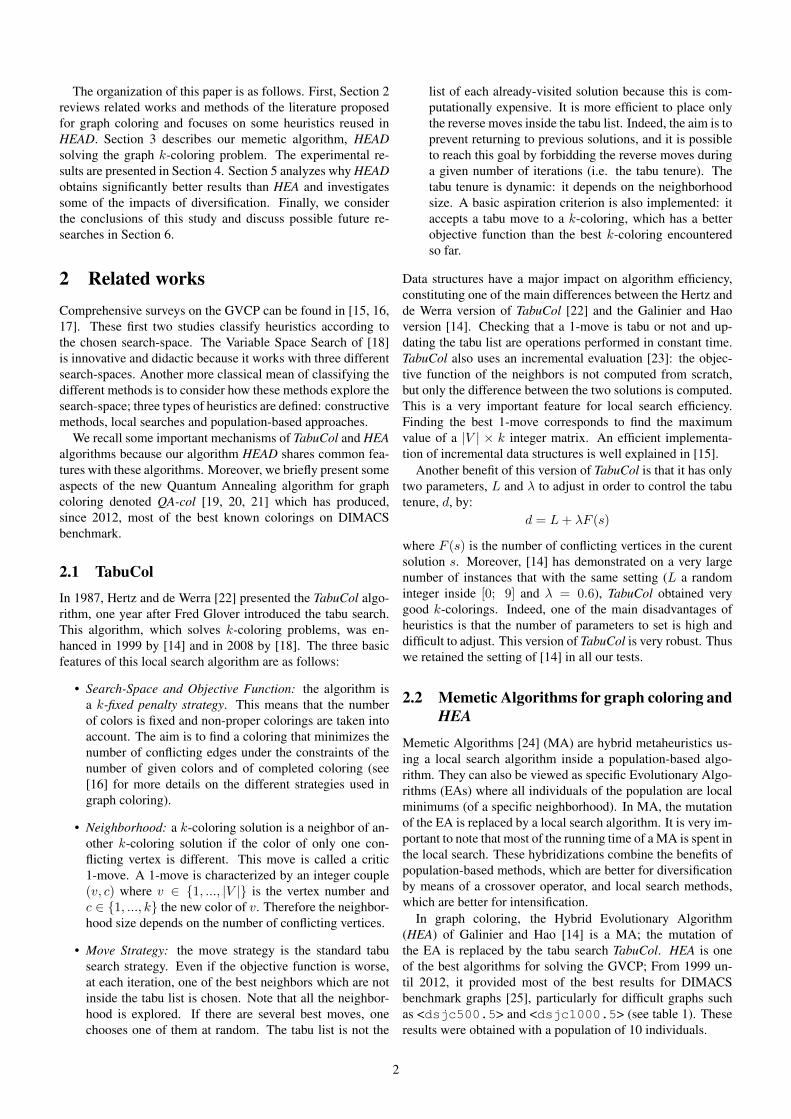
Table 1 presents results of the principal methods known todate for 19 difficult graphs. For each graph, the lowest numberof colors found by each algorithm is indicated (upper bound ofχ). For TabuCol [22] the reported results are from [18] (2008)which are better than those of 1987. The most recent algo-rithms, QA-col (Quantum Annealing for graph coloring [21])and IE2COL (Improving the Extraction and Expansion methodfor large graph COLoring [26]), provide the best results butQA-col is based on a cluster of PC using 10 processing coressimultaneously and IE2COL is profiled for large graphs (> 900vertices). Note that HEA [14], AmaCol [27], MACOL [28],EXTRACOL [29] and IE2COL are also population-based algo-rithms using TabuCol and GPX crossover or an improvementof GPX (GPX with n > 2 parents for MACOL and EXTRACOLand the GPX process is replaced in AmaCol by a selection of kcolor classes among a very large pool of color classes). OnlyQA-col has another approach based on several parallel simu-lated annealing algorithms interacting together with an attrac-tive/repulsive process (cf. section 2.3).

1ftp://dimacs.rutgers.edu/pub/challenge/graph/benchmarks/color/

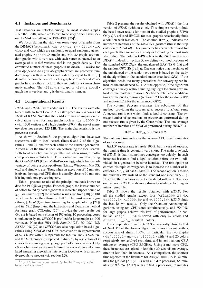
Table 2 presents the results obtained with HEAD’, the firstversion of HEAD (without elite). This simplest version findsthe best known results for most of the studied graphs (13/19);Only QA-col (and IE2COL for <C> graphs) occasionally findsa solution with less color. The column IterTC indicates thenumber of iterations of the TabuCol algorithm (this is the stopcriterion of TabuCol). This parameter has been determined foreach graph after an empirical analysis for finding the most suit-able value. The column GPX refers to the GPX used insideHEAD’. Indeed, in section 5, we define two modifications ofthe standard GPX (Std): the unbalanced GPX (U([0 ; 1])) andthe random GPX (R(J0 ; kK)). One can notice that the choice ofthe unbalanced or the random crossover is based on the studyof the algorithm in the standard mode (standard GPX). If thealgorithm needs too many generations for converging we in-troduce the unbalanced GPX. At the opposite, if the algorithmconverges quickly without finding any legal k-coloring we in-troduce the random crossover. Section 5 details the modifica-tions of the GPX crossover (section 5.2.1 for the random GPXand section 5.2.2 for the unbalanced GPX).

The column Success evaluates the robustness of thismethod, providing the success rate: success_runs/total_runs.A success run is one which finds a legal k-coloring. The av-erage number of generations or crossovers performed duringone success run is given by the Cross value. The total averagenumber of iterations of TabuCol preformed during HEAD’ is

Iter = IterTC ×Cross× 2.

The column Time indicates the average CPU time in minutesof success runs.

HEAD’ success rate is rarely 100%, but in case of success,the running time is generally very short. The main drawbackof HEAD’ is that it sometimes converges too quickly. In suchinstances it cannot find a legal solution before the two indi-viduals in a generation become identical. The first option tocorrect this rapid convergence, is to increase the number of it-erations IterTC of each TabuCol. The second option is to usethe random GPX instead of the standard one (section 5.2.1).However, these options are not considered sufficient. The sec-ond version, HEAD, adds more diversity while performing anintensifying role.

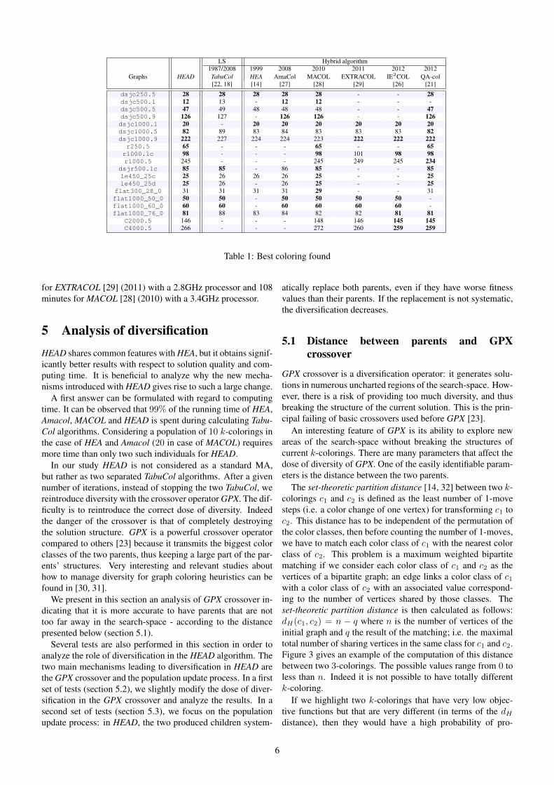
Table 3 shows the results obtained with HEAD. Forall the studied graphs except four (<flat300_28_0>,<r1000.5>, <C2000.5> and <C4000.5>), HEAD findsthe best known results. Only the Quantum Annealing al-gorithm, using ten CPU cores simultaneously, and IE2COLfor large graphs, achieve this level of performance. In par-ticular, <dsjc500.5> is solved with only 47 colors and<flat1000_76_0> with 81 colors.

The computation time of HEAD is generally close to thatof HEAD’ but the former algorithm is more robust with asuccess rate of almost 100%. In particular, the two graphs<dsjc500.5> and <dsjc1000.1> with 48 and 20 colorsrespectively are resolved each time, and in less than one CPUminute on average (CPU 3.3GHz). Using a multicore CPU,these instances are solved in less than 30 seconds on average,often in less than 10 seconds. As a comparison, the shortesttime reported in the literature for <dsjc1000.1> is 32 min-utes for QA-col [20] (2011) with a 3GHz processor, 65 min-utes for IE2COL (2012) with a 2.8GHz processor, 93 minutes

5

LS Hybrid algorithm1987/2008 1999 2008 2010 2011 2012 2012

Graphs HEAD TabuCol HEA AmaCol MACOL EXTRACOL IE2COL QA-col[22, 18] [14] [27] [28] [29] [26] [21]

dsjc250.5 28 28 28 28 28 - - 28dsjc500.1 12 13 - 12 12 - - -dsjc500.5 47 49 48 48 48 - - 47dsjc500.9 126 127 - 126 126 - - 126dsjc1000.1 20 - 20 20 20 20 20 20dsjc1000.5 82 89 83 84 83 83 83 82dsjc1000.9 222 227 224 224 223 222 222 222r250.5 65 - - - 65 - - 65r1000.1c 98 - - - 98 101 98 98r1000.5 245 - - - 245 249 245 234

dsjr500.1c 85 85 - 86 85 - - 85le450_25c 25 26 26 26 25 - - 25le450_25d 25 26 - 26 25 - - 25

flat300_28_0 31 31 31 31 29 - - 31flat1000_50_0 50 50 - 50 50 50 50 -flat1000_60_0 60 60 - 60 60 60 60 -flat1000_76_0 81 88 83 84 82 82 81 81

C2000.5 146 - - - 148 146 145 145C4000.5 266 - - - 272 260 259 259

Table 1: Best coloring found

for EXTRACOL [29] (2011) with a 2.8GHz processor and 108minutes for MACOL [28] (2010) with a 3.4GHz processor.

5 Analysis of diversificationHEAD shares common features with HEA, but it obtains signif-icantly better results with respect to solution quality and com-puting time. It is beneficial to analyze why the new mecha-nisms introduced with HEAD gives rise to such a large change.

A first answer can be formulated with regard to computingtime. It can be observed that 99% of the running time of HEA,Amacol, MACOL and HEAD is spent during calculating Tabu-Col algorithms. Considering a population of 10 k-colorings inthe case of HEA and Amacol (20 in case of MACOL) requiresmore time than only two such individuals for HEAD.

In our study HEAD is not considered as a standard MA,but rather as two separated TabuCol algorithms. After a givennumber of iterations, instead of stopping the two TabuCol, wereintroduce diversity with the crossover operator GPX. The dif-ficulty is to reintroduce the correct dose of diversity. Indeedthe danger of the crossover is that of completely destroyingthe solution structure. GPX is a powerful crossover operatorcompared to others [23] because it transmits the biggest colorclasses of the two parents, thus keeping a large part of the par-ents’ structures. Very interesting and relevant studies abouthow to manage diversity for graph coloring heuristics can befound in [30, 31].

We present in this section an analysis of GPX crossover in-dicating that it is more accurate to have parents that are nottoo far away in the search-space - according to the distancepresented below (section 5.1).

Several tests are also performed in this section in order toanalyze the role of diversification in the HEAD algorithm. Thetwo main mechanisms leading to diversification in HEAD arethe GPX crossover and the population update process. In a firstset of tests (section 5.2), we slightly modify the dose of diver-sification in the GPX crossover and analyze the results. In asecond set of tests (section 5.3), we focus on the populationupdate process: in HEAD, the two produced children system-

atically replace both parents, even if they have worse fitnessvalues than their parents. If the replacement is not systematic,the diversification decreases.

5.1 Distance between parents and GPXcrossover

GPX crossover is a diversification operator: it generates solu-tions in numerous uncharted regions of the search-space. How-ever, there is a risk of providing too much diversity, and thusbreaking the structure of the current solution. This is the prin-cipal failing of basic crossovers used before GPX [23].

An interesting feature of GPX is its ability to explore newareas of the search-space without breaking the structures ofcurrent k-colorings. There are many parameters that affect thedose of diversity of GPX. One of the easily identifiable param-eters is the distance between the two parents.

The set-theoretic partition distance [14, 32] between two k-colorings c1 and c2 is defined as the least number of 1-movesteps (i.e. a color change of one vertex) for transforming c1 toc2. This distance has to be independent of the permutation ofthe color classes, then before counting the number of 1-moves,we have to match each color class of c1 with the nearest colorclass of c2. This problem is a maximum weighted bipartitematching if we consider each color class of c1 and c2 as thevertices of a bipartite graph; an edge links a color class of c1with a color class of c2 with an associated value correspond-ing to the number of vertices shared by those classes. Theset-theoretic partition distance is then calculated as follows:dH(c1, c2) = n − q where n is the number of vertices of theinitial graph and q the result of the matching; i.e. the maximaltotal number of sharing vertices in the same class for c1 and c2.Figure 3 gives an example of the computation of this distancebetween two 3-colorings. The possible values range from 0 toless than n. Indeed it is not possible to have totally differentk-coloring.

If we highlight two k-colorings that have very low objec-tive functions but that are very different (in terms of the dHdistance), then they would have a high probability of pro-

6

Instances k IterTC GPX Success Iter Cross Timedsjc250.5 28 6000 Std 17/20 1× 106 79 0.01 mindsjc500.1 12 8000 Std 15/20 2.5× 106 158 0.03 mindsjc500.5 48 8000 Std 9/20 5.3× 106 334 0.2 mindsjc500.9 126 25000 Std 10/20 2.5× 107 517 1 mindsjc1000.1 20 7000 Std 7/20 8.2× 106 588 0.2 mindsjc1000.5 83 40000 Std 16/20 1.37× 108 1723 10 mindsjc1000.9 222 60000 Std 1/20 4.45× 108 3711 33 min

223 30000 Std 4/20 6.6× 107 1114 5 minr250.5 65 12000 Std 1/20 8.11× 108 33828 12 min

65 2000 R(20) 6/20 5.31× 108 132773 10 minr1000.1c 98 65000 Std 1/20 2.32× 106 18 0.1 min

98 25000 R(98) 20/20 6.5× 106 130 0.4 minr1000.5 245 360000 Std 20/20 2.6× 109 3636 135 min

245 240000 U(0.98) 17/20 6.48× 108 1352 39 mindsjr500.1c 85 4200000 Std 1/20 5.8× 106 1 0.2 min

85 1000 R(85) 13/20 5× 105 279 0.02 minle450_25c 25 21000000 Std 20/20 3.5× 109 57 38 min

25 300000 U(0.98) 10/20 2.86× 108 477 2.4 minle450_25d 25 21000000 Std 20/20 5.7× 109 135 64 min

25 340000 U(0.98) 10/20 2.15× 108 317 2 minflat300_28_0 31 4000 Std 20/20 1× 106 117 0.02 minflat1000_50_0 50 130000 Std 20/20 1.1× 106 4 0.3 minflat1000_60_0 60 130000 Std 20/20 2.3× 106 9 0.5 minflat1000_76_0 81 40000 Std 1/20 1.49× 109 18577 137 min

82 40000 Std 18/20 1.57× 108 1969 11 minC2000.5 148 140000 Std 10/10 1.7× 109 6308 794 minC4000.5 275 140000 Std 8/10 1.1× 109 4091 3496 min

Table 2: Results of HEAD’, the first version of HEAD algorithm (without elites)

11

1

A B C C D E G

color class blue D E F G

color class green H I J

A F I

B H J

color class red 1

1

2

3color class red

coloring 1 coloring 2

Figure 3: A graph with 10 vertices (A, B, C, D, E, F, G, H, Iand J), three colors (red, blue and green) and two 3-colorings:coloring 1 and coloring 2. We defined the weighted bipartitegraph corresponding to the number of vertices shared by colorclasses of coloring 1 and coloring 2. The bold lines correspondto the maximum weighted bipartite matching. The maximaltotal number of sharing vertices in the same class is equal toq = 3 + 2 + 1 = 6. Then the set-theoretic partition distancebetween those two 3-colorings is equal to: dH(coloring 1, col-oring 2) = n− q = 10− 6 = 4. This distance is independentof the permutation of the color classes.

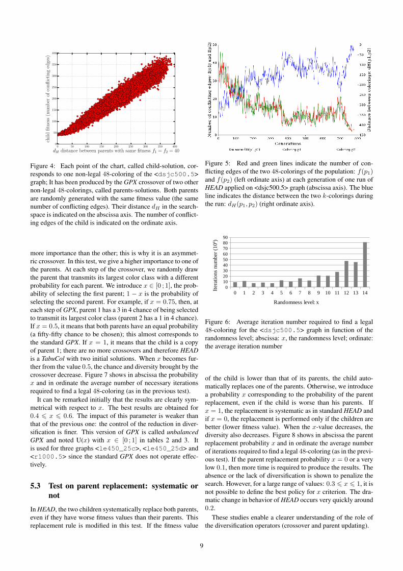
ducing children with very high objective functions followingcrossover. The danger of the crossover is of completely de-stroying the k-coloring structure. On the other hand, two veryclose k-colorings (in terms of the dH distance) produce a childwith an almost identical objective function. Chart 4 shows thecorrelation between the distance separating two k-coloringshaving the same number of conflicting edges (objective func-tions equal to 40) and the number of conflicting edges of thechild produced after GPX crossover. This chart is obtainedconsidering k = 48 colors into the <dsjc500.5> graph.More precisely, this chart results of the following steps: 1)First, 100 non legal 48-colorings, called parents, are randomlygenerated with a fitness (that is a number of conflicting edges)equal to 40. Tabucol algorithm is used to generate these 100

parents (Tabucol is stopped when exactly 40 conflicted edgesare found). 2) A GPX crossover is performed on all possiblepairs of parents, generating for each pair two new non legal48-colorings, called children. Indeed, GPX is asymmetrical,then the order of the parents is important. By this way, 9900(= 100× 99) children are generated. 3) We perform twice thesteps 1) and 2), therefore the total number of generated chil-dren is equal to 19800. Each point of the chart corresponds toone child. The y-axis indicates the fitness of the child. Thex-axis indicates the distance dH in the search-space betweenthe two parents of the child. There is a quasi-linear correlationbetween these two parameters (Pearson correlation coefficientequals to 0.973). Moreover, chart 4 shows that a crossovernever improves a k-coloring. As stated in section 2.2, thelast step of GPX produces many conflicts. Indeed, if the twoparents are very far in terms of dH , then a large number of ver-tices remain uncolored at the final step of GPX. Those verticesare then randomly added to the color classes, producing manyconflicting edges in the offspring. This explains why in MA, alocal search always follows a crossover operator.

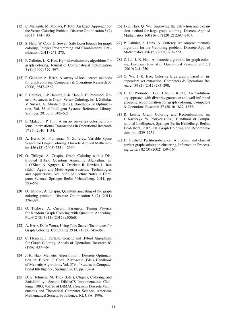
Figure 5 presents the evolution of the objective function (i.e.the number of conflicting edges) of the two k-colorings of thepopulation at each generation of HEAD. It also indicates thedH distance between the two k-colorings. This figure is ob-tained by considering one typical run to find one 48-coloringof <dsjc500.5> graph. The objective function of the twok-colorings (f(p1) and f(p2)) are very close during the wholerun: the average of the difference f(p1) − f(p2) on the 779generations is equal to−0.11 with a variance of 2.44. Figure 5shows that there is a significant correlation between the qual-ity of the two k-colorings (in terms of fitness values) and thedistance dH between them before the GPX crossover: the Pear-son correlation coefficient is equal to 0.927 (respectively equalto 0.930) between f(p1) and dH(p1, p2) (resp. between f(p2)

7

Instances k IterTC GPX Success Iter Cross Timedsjc250.5 28 6000 Std 20/20 9× 105 77 0.01 mindsjc500.1 12 4000 Std 20/20 3.8× 106 483 0.1 mindsjc500.5 47 8000 Std 2/10000 2.4× 107 1517 0.8 min

48 8000 Std 20/20 7.6× 106 479 0.2 mindsjc500.9 126 15000 Std 13/20 2.9× 107 970 1.2 mindsjc1000.1 20 3000 Std 20/20 3.4× 106 567 0.2 mindsjc1000.5 82 60000 Std 3/20 1× 109 8366 48 min

83 40000 Std 20/20 9.6× 107 1200 6 mindsjc1000.9 222 50000 Std 2/20 1.2× 109 11662 86 min

223 30000 Std 19/20 1.26× 108 2107 10 minr250.5 65 10000 Std 1/20 6.98× 108 34898 13 min

65 4000 R(20) 20/20 3.91× 108 48918 6.3 minr1000.1c 98 45000 Std 3/20 3.7× 106 42 0.2 min

98 25000 R(98) 20/20 3.9× 106 78 0.24 minr1000.5 245 360000 Std 20/20 4.6× 109 6491 244 min

245 240000 U(0.98) 20/20 5.3× 108 1104 25 mindsjr500.1c 85 4200000 Std 1/20 5.8× 106 1 0.2 min

85 400 R(85) 20/20 4× 105 408 0.02 minle450_25c 25 22000000 Std 20/20 2.7× 109 62 30 min

25 220000 U(0.98) 20/20 3.89× 108 885 5 minle450_25d 25 21000000 Std 20/20 7× 109 161 90 min

25 220000 U(0.98) 20/20 2.35× 108 534 2 minflat300_28_0 31 4000 Std 20/20 9× 105 120 0.02 minflat1000_50_0 50 130000 Std 20/20 1.2× 106 5 0.3 minflat1000_60_0 60 130000 Std 20/20 2.3× 106 9 0.5 minflat1000_76_0 81 60000 Std 3/20 1× 109 8795 60 min

82 40000 Std 20/20 8.4× 107 1052 5 minC2000.5 146 140000 Std 8/10 1.78× 109 6358 281 min

147 140000 Std 10/10 7.26× 108 2595 124 minC4000.5 266 140000 Std 4/10 2.5× 109 9034 1923 min

267 140000 Std 8/10 1.6× 109 5723 1433 min

Table 3: Results of the second version of HEAD algorithm (with elites) including the indication of CPU time

and dH(p1, p2)). Those plots give the main key for understand-ing why HEAD is more effective than HEA: the linear anti-correlation between the two k-colorings with approximatelysame objective function values f(p1) ' f(p2) is around equalto 500−10 × dH(p1, p2). The same level of correlation witha population of 10 individuals using HEA cannot be obtainedexcept with sophisticated sharing process.

Diversity is necessary when an algorithm is trapped in a lo-cal minimum but diversity should be avoided in other case.The next subsections analyze several levers which may able toincrease or decrease the diversity in HEAD.

5.2 Dose of diversification in the GPX crossover

Some modifications are performed on the GPX crossover inorder to increase (as for the first test) or decrease (as for thesecond test) the dose of diversification within this operator.

5.2.1 Test on GPX with increased randomness: randomdraw of a number of color classes

In order to increase the level of randomness within the GPXcrossover, we randomize the GPX. It should be remembered(cf. section 2.2) that at each step of the GPX, the selected par-ent transmits the largest color class to the child. In this test,we begin by randomly transmitting x ∈ J0 ; kK color classeschosen from the parents to the child; after those x steps, westart again by alternately transmitting the largest color classfrom each parent (x is the random level). If x = 0, then thecrossover is the same as the initial GPX. If x increases, thenthe randomness and the diversity also increase. To evaluate

this modification of the crossover, we count the cumulative it-erations number of TabuCol that one HEAD run requires inorder to find a legal k-coloring. For each x value, the algo-rithm is run ten times in order to produce more robust results.For the test, we consider the 48-coloring problem for graph<dsjc500.5> of the DIMACS benchmark. Figure 6 showsin abscissa the random level x and in ordinate the average num-ber of iterations required to find a legal 48-coloring.

First, 0 6 x 6 k, where k is the number of colors, butwe stop the computation for x > 15, because from x = 15,the algorithm does not find a 48-coloring within an acceptablecomputing time limit. This means that when we introduce toomuch diversification, the algorithm cannot find a legal solution.Indeed, for a high x value, the crossover does not transmit thegood features of the parents, therefore the child appears to be arandom initial solution. When 0 6 x 6 8, the algorithm findsa legal coloring in more or less 10 million iterations. It is noteasy to decide which x-value obtains the quickest result. How-ever this parameter enables an increase of diversity in HEAD.This version of GPX is called random GPX and noted R(x)with x ∈ J0 ; kK in tables 2 and 3. It is used for three graphs<r250.5>, <r1000.1c> and <dsjr500.1c> because thestandard GPX does not operate effectively. The fact that thesethree graphs are more structured that the others may explainwhy the random GPX works better.

5.2.2 Test on GPX with decreased randomness: imbal-anced crossover

In the standard GPX, the role of each parent is balanced: theyalternatively transmit their largest color class to the child. Ofcourse, the parent which first transmits its largest class, has

8

0 50 100 150 200 250 300 350 400

dH distance between parents with same fitness f1 = f2 = 40

0

50

100

150

200

250

300

350

400

child

fitn

ess

(nu

mb

erof

con

flict

ing

edge

s)

Figure 4: Each point of the chart, called child-solution, cor-responds to one non-legal 48-coloring of the <dsjc500.5>graph; It has been produced by the GPX crossover of two othernon-legal 48-colorings, called parents-solutions. Both parentsare randomly generated with the same fitness value (the samenumber of conflicting edges). Their distance dH in the search-space is indicated on the abscissa axis. The number of conflict-ing edges of the child is indicated on the ordinate axis.

more importance than the other; this is why it is an asymmet-ric crossover. In this test, we give a higher importance to one ofthe parents. At each step of the crossover, we randomly drawthe parent that transmits its largest color class with a differentprobability for each parent. We introduce x ∈ [0 ; 1], the prob-ability of selecting the first parent; 1 − x is the probability ofselecting the second parent. For example, if x = 0.75, then, ateach step of GPX, parent 1 has a 3 in 4 chance of being selectedto transmit its largest color class (parent 2 has a 1 in 4 chance).If x = 0.5, it means that both parents have an equal probability(a fifty-fifty chance to be chosen); this almost corresponds tothe standard GPX. If x = 1, it means that the child is a copyof parent 1; there are no more crossovers and therefore HEADis a TabuCol with two initial solutions. When x becomes fur-ther from the value 0.5, the chance and diversity brought by thecrossover decrease. Figure 7 shows in abscissa the probabilityx and in ordinate the average number of necessary iterationsrequired to find a legal 48-coloring (as in the previous test).

It can be remarked initially that the results are clearly sym-metrical with respect to x. The best results are obtained for0.4 6 x 6 0.6. The impact of this parameter is weaker thanthat of the previous one: the control of the reduction in diver-sification is finer. This version of GPX is called unbalancedGPX and noted U(x) with x ∈ [0 ; 1] in tables 2 and 3. Itis used for three graphs <le450_25c>, <le450_25d> and<r1000.5> since the standard GPX does not operate effec-tively.

5.3 Test on parent replacement: systematic ornot

In HEAD, the two children systematically replace both parents,even if they have worse fitness values than their parents. Thisreplacement rule is modified in this test. If the fitness value

Figure 5: Red and green lines indicate the number of con-flicting edges of the two 48-colorings of the population: f(p1)and f(p2) (left ordinate axis) at each generation of one run ofHEAD applied on <dsjc500.5> graph (abscissa axis). The blueline indicates the distance between the two k-colorings duringthe run: dH(p1, p2) (right ordinate axis).

Figure 6: Average iteration number required to find a legal48-coloring for the <dsjc500.5> graph in function of therandomness level; abscissa: x, the randomness level; ordinate:the average iteration number

of the child is lower than that of its parents, the child auto-matically replaces one of the parents. Otherwise, we introducea probability x corresponding to the probability of the parentreplacement, even if the child is worse than his parents. Ifx = 1, the replacement is systematic as in standard HEAD andif x = 0, the replacement is performed only if the children arebetter (lower fitness value). When the x-value decreases, thediversity also decreases. Figure 8 shows in abscissa the parentreplacement probability x and in ordinate the average numberof iterations required to find a legal 48-coloring (as in the previ-ous test). If the parent replacement probability x = 0 or a verylow 0.1, then more time is required to produce the results. Theabsence or the lack of diversification is shown to penalize thesearch. However, for a large range of values: 0.3 6 x 6 1, it isnot possible to define the best policy for x criterion. The dra-matic change in behavior of HEAD occurs very quickly around0.2.

These studies enable a clearer understanding of the role ofthe diversification operators (crossover and parent updating).

9

Figure 7: Average number of iterations required to find a le-gal 48-coloring for <dsjc500.5> graph according to the im-balanced crossover; abscissa: x, probability to select the firstparent at each step of GPX; ordinate: average iteration number

Figure 8: Average number of iterations required to find a legal48-coloring for <dsjc500.5> graph in function of the par-ents’ replacement policy; abscissa: parent replacement proba-bility; ordinate: average number of iterations

The criteria presented here, such as the random level of thecrossover or the imbalanced level of the crossover, have showntheir efficiency on some graphs. These GPX modificationscould successfully be applied into future algorithms in order tomanage the diversity dynamically.

6 ConclusionWe proposed a new algorithm for the graph coloring prob-lem, called HEAD. This memetic algorithm combines the localsearch algorithm TabuCol as an intensification operator withthe crossover operator GPX as a way to escape from local min-ima. Its originality is that it works with a simple populationof only two individuals. In order to prevent premature conver-gence, the proposed approach introduces an innovative way formanaging the diversification based on elite solutions.

The computational experiments, carried out on a set ofchallenging DIMACS graphs, show that HEAD produces ac-curate results, such as 222-colorings for <dsjc1000.9>,81-colorings for <flat1000_76_0> and even 47-coloringsfor <dsjc500.5> and 82-colorings for <dsjc1000.5>,which have up to this point only been found by quantum an-nealing [21] with a massive multi-CPU. The results achieved

by HEAD let us think that this scheme could be successfullyapplied to other problems, where a stochastic or asymmetriccrossover can be defined.

We performed an in-depth analysis on the crossover opera-tor in order to better understand its role in the diversificationprocess. Some interesting criteria have been identified, suchas the crossover’s levels of randomness and imbalance. Thosecriteria pave the way for further researches.

References[1] K. Aardal, S. Hoesel, A. Koster, C. Mannino, A. Sassano,

Models and solution techniques for frequency assign-ment problems, Quarterly Journal of the Belgian, Frenchand Italian Operations Research Societies 1 (4) (2003)261–317.

[2] M. Dib, A. Caminada, H. Mabed, Frequency manage-ment in Radio military Networks, in: INFORMS Tele-com 2010, 10th INFORMS Telecommunications Confer-ence, Montreal, Canada, 2010.

[3] F. T. Leighton, A Graph Coloring Algorithm for LargeScheduling Problems, Journal of Research of the Na-tional Bureau of Standards 84 (6) (1979) 489–506.

[4] N. Zufferey, P. Amstutz, P. Giaccari, Graph ColouringApproaches for a Satellite Range Scheduling Problem,Journal of Scheduling 11 (4) (2008) 263 – 277.

[5] D. C. Wood, A Technique for Coloring a Graph Appli-cable to Large-Scale Timetabling Problems, ComputerJournal 12 (1969) 317–322.

[6] N. Barnier, P. Brisset, Graph Coloring for Air Traf-fic Flow Management, Annals of Operations Research130 (1-4) (2004) 163–178.

[7] C. Allignol, N. Barnier, A. Gondran, Optimized FlightLevel Allocation at the Continental Scale, in: Inter-national Conference on Research in Air Transporta-tion (ICRAT 2012), Berkeley, California, USA, 22-25/05/2012, 2012.

[8] M. R. Garey, D. S. Johnson, Computers and Intractabil-ity: A Guide to the Theory of NP-Completeness, Free-man, San Francisco, CA, USA, 1979.

[9] R. Karp, Reducibility among combinatorial problems, in:R. E. Miller, J. W. Thatcher (Eds.), Complexity of Com-puter Computations, Plenum Press, New York, USA,1972, pp. 85–103.

[10] D. S. Johnson, C. R. Aragon, L. A. McGeoch,C. Schevon, Optimization by Simulated Annealing: AnExperimental Evaluation; Part II, Graph Coloring andNumber Partitioning, Operations Research 39 (3) (1991)378–406.

[11] N. Dubois, D. de Werra, Epcot: An efficient procedurefor coloring optimally with Tabu Search, Computers &Mathematics with Applications 25 (10–11) (1993) 35–45.

10

[12] E. Malaguti, M. Monaci, P. Toth, An Exact Approach forthe Vertex Coloring Problem, Discrete Optimization 8 (2)(2011) 174–190.

[13] S. Held, W. Cook, E. Sewell, Safe lower bounds for graphcoloring, Integer Programming and Combinatoral Opti-mization (2011) 261–273.

[14] P. Galinier, J.-K. Hao, Hybrid evolutionary algorithms forgraph coloring, Journal of Combinatorial Optimization3 (4) (1999) 379–397.

[15] P. Galinier, A. Hertz, A survey of local search methodsfor graph coloring, Computers & Operations Research 33(2006) 2547–2562.

[16] P. Galinier, J.-P. Hamiez, J.-K. Hao, D. C. Porumbel, Re-cent Advances in Graph Vertex Coloring, in: I. Zelinka,V. Snásel, A. Abraham (Eds.), Handbook of Optimiza-tion, Vol. 38 of Intelligent Systems Reference Library,Springer, 2013, pp. 505–528.

[17] E. Malaguti, P. Toth, A survey on vertex coloring prob-lems, International Transactions in Operational Research17 (1) (2010) 1–34.

[18] A. Hertz, M. Plumettaz, N. Zufferey, Variable SpaceSearch for Graph Coloring, Discrete Applied Mathemat-ics 156 (13) (2008) 2551 – 2560.

[19] O. Titiloye, A. Crispin, Graph Coloring with a Dis-tributed Hybrid Quantum Annealing Algorithm, in:J. O’Shea, N. Nguyen, K. Crockett, R. Howlett, L. Jain(Eds.), Agent and Multi-Agent Systems: Technologiesand Applications, Vol. 6682 of Lecture Notes in Com-puter Science, Springer Berlin / Heidelberg, 2011, pp.553–562.

[20] O. Titiloye, A. Crispin, Quantum annealing of the graphcoloring problem, Discrete Optimization 8 (2) (2011)376–384.

[21] O. Titiloye, A. Crispin, Parameter Tuning Patternsfor Random Graph Coloring with Quantum Annealing,PLoS ONE 7 (11) (2012) e50060.

[22] A. Hertz, D. de Werra, Using Tabu Search Techniques forGraph Coloring, Computing 39 (4) (1987) 345–351.

[23] C. Fleurent, J. Ferland, Genetic and Hybrid Algorithmsfor Graph Coloring, Annals of Operations Research 63(1996) 437–464.

[24] J.-K. Hao, Memetic Algorithms in Discrete Optimiza-tion, in: F. Neri, C. Cotta, P. Moscato (Eds.), Handbookof Memetic Algorithms, Vol. 379 of Studies in Computa-tional Intelligence, Springer, 2012, pp. 73–94.

[25] D. S. Johnson, M. Trick (Eds.), Cliques, Coloring, andSatisfiability: Second DIMACS Implementation Chal-lenge, 1993, Vol. 26 of DIMACS Series in Discrete Math-ematics and Theoretical Computer Science, AmericanMathematical Society, Providence, RI, USA, 1996.

[26] J.-K. Hao, Q. Wu, Improving the extraction and expan-sion method for large graph coloring, Discrete AppliedMathematics 160 (16–17) (2012) 2397–2407.

[27] P. Galinier, A. Hertz, N. Zufferey, An adaptive memoryalgorithm for the k-coloring problem, Discrete AppliedMathematics 156 (2) (2008) 267–279.

[28] Z. Lü, J.-K. Hao, A memetic algorithm for graph color-ing, European Journal of Operational Research 203 (1)(2010) 241–250.

[29] Q. Wu, J.-K. Hao, Coloring large graphs based on in-dependent set extraction, Computers & Operations Re-search 39 (2) (2012) 283–290.

[30] D. C. Porumbel, J.-K. Hao, P. Kuntz, An evolution-ary approach with diversity guarantee and well-informedgrouping recombination for graph coloring, Computers& Operations Research 37 (2010) 1822–1832.

[31] R. Lewis, Graph Coloring and Recombination, in:J. Kacprzyk, W. Pedrycz (Eds.), Handbook of Compu-tational Intelligence, Springer Berlin Heidelberg, Berlin,Heidelberg, 2015, Ch. Graph Coloring and Recombina-tion, pp. 1239–1254.

[32] D. Gusfield, Partition-distance: A problem and class ofperfect graphs arising in clustering, Information Process-ing Letters 82 (3) (2002) 159–164.

11