Variational Monte Carlo Method for Fermions

Vijay B. Shenoy

shenoy@physics.iisc.ernet.in

Indian Institute of Science, Bangalore

December 26, 2009

1 / 91

Acknowledgements

Sandeep Pathak

Department of Science and Technology

2 / 91

Plan of the Lectures on Variational Monte Carlo Method

Motivation, Overview and Key Ideas

Details of VMC

Application to Superconductivity

3 / 91

The Strongly Correlated Panorama...Fig. 1. Phase diagramsof representativemateri-als of the strongly cor-related electron family(notations are standardand details can be foundin the original refer-ences). (A) Temperatureversus hole density phasediagram of bilayer man-ganites (74), includingseveral types of antiferro-magnetic (AF) phases, aferromagnetic (FM)phase, and even a glob-ally disordered region atx 0 0.75. (B) Genericphase diagram for HTSC.SG stands for spin glass.(C) Phase diagram ofsingle layered ruthenates(75, 76), evolving froma superconducting (SC)state at x 0 2 to an AFinsulator at x 0 0 (xcontrols the bandwidthrather than the carrierdensity). Ruthenatesare believed to be cleanmetals at least at largex, thus providing afamily of oxides wherecompetition and com-plexity can be studiedwith less quenched dis-order than in Mn ox-ides. (D) Phase diagramof Co oxides (77), withSC, charge-ordered (CO),and magnetic regimes.(E) Phase diagram ofthe organic k-(BEDT-TTF)2Cu[N(CN)2]Cl salt(57). The hatched re-gion denotes the co-existence of metal andinsulator phases. (F)Schematic phase dia-gram of the Ce-basedheavy fermion materials(51).

(Dagotto, Science, (2005))

4 / 91

...and now, Cold Atom Quantum Simulators

(Bloch et al., RMP, (2009))

Hamiltonian...for here, or to go?

5 / 91

The Strategy

Identify “key degrees of freedom” of the system of interest

Identify the key interactions

Write a Hamiltonian (eg. tJ-model)...reduce the problem to a model

“Solve” the Hamiltonian

....

Nature(Science)/Nature Physics/PRL/PRB...

6 / 91

“Solvers”

Mean Field Theories (MFT)

Slave Particle Theories (and associated MFTs)

Dynamical Mean Field Theories (DMFT)

Exact Diagonalization

Quantum Monte Carlo Methods (eg. Determinental)

Variational Monte Carlo (VMC)

...

AdS/CFT

7 / 91

Great Expectations

Prerequisites

Graduate quantum mechanics including “second quantization”

Ideas of “Mean Field Theory”

Some familiarity with “classical” superconductivity

At the end of the lectures, youcan/will have

Understood concepts of VMC

Know-how to write your owncode

A free code (pedestrianVMC)

Seen examples of VMC instrongly correlated systems

8 / 91

References

NATO Series Lecture Notes by Nightingale, Umrigar, seehttp://www.phys.uri.edu/˜nigh/QMC-NATO/webpage/abstracts/lectures.html

Morningstar, hep-lat/070202

Ceperley, Chester and Kalos, PRB 17, 3081 (1977)

9 / 91

VMC in a Nutshell

Strategy to study ground (and some special excited) state(s)

“Guess” the ground state

Use Schrodinger’s variational principle to optimize the ground state

Calculate observables of interest with the optimal state

...

10 / 91

Hall of Fame

Bardeen, Cooper, Schrieffer Laughlin

Quote/Question from A2Z, Plain Vanilla JPCM (2004)

The philosophy of this method (VMC )is analogous to that used by BCS forsuperconductivity, and by Laughlin for the fractional quantum Hall effect:simply guess a wavefunction. Is there any better way to solve anon-perturbative many-body problem?

11 / 91

Variational Principle

Eigenstates of the Hamiltonian satisfy

H|Ψ〉 = E |Ψ〉

where E is the energy eigenvalue

Alternate way of stating this◮ Define an “energy functional” for any given state |Φ〉

E [Φ] = 〈Φ|H|Φ〉

◮ Among all states |Φ〉 that satisfy 〈Φ|Φ〉 = 1, those that extremize E [Φ]are eigenstates of H Exercise: Prove this!

◮ The state(s) that minimises(minimise) E [Φ] is(are) the ground state(s)

12 / 91

Variational Principle in Action...A Simple Example

Ground state H+2 molecule with a given nuclear separation

“Guess” the wave function (linear combination of atomic orbitals)

|ψ〉 = a|1〉+ b|2〉

where |1, 2〉 are atomic orbitals centered around protons 1 and 2

Find energy function (taking everything real)

E (a, b) = H11a2 + 2H12ab + H22b

2

(symbols have obvious meaning)

Minimize (with appropriate constraints) to find |ψ〉g = 1√2(|1〉+ |2〉)

(for H12 < 0) Question: Is this the actual ground state?

Example shows key ideas (and limitations) of the variational approach!

13 / 91

Variational Approach in Many Body Physics

Guess the ground state wavefunction |Ψ〉|Ψ〉 depends on some variational parameters α1, α2... which “containthe physics” of the wavefunction

◮ Example,

|BCS〉 =

[∏

k

(

uk + vkc†k↑c

†−k↓

)]

|0〉

uk , vk are the “αi s”

In general, αi s are chosen◮ To realize some sort of “order” or “broken symmetry”, (for example,

magnetic order)...there could be more than one order present (forexample, superconductivity and magnetism)

◮ To enforce some sort of “correlation” that we “simply” know exists

and can include all of the “effects” above

...your guess is not as good as mine!

14 / 91

Variational Principle vs. MFT

Mean Field theory◮ Replace H by HMF which is usually quadratic◮ Use the Feynman identity F ≤ FMF + 〈H − HMF 〉MF (F is free energy)◮ Kills “fluctuations”

Variational Principle◮ Works with the full Hamiltonian◮ Non-perturbative◮ Well designed wavefunctions can include fluctuations above MFT

Usually MFT provides us with intuitive starting point...we can then“well design” the variational wavefunction to include the fluctuationsthat we miss

15 / 91

Overall Strategy of Variational Approach

Summary of Variational Approach

1 Design a ground state |Ψ(αi )〉2 Energy function

E (αi ) =〈Ψ(αi )|H|Ψ(αi )〉〈Ψ(αi )|Ψ(αi )〉

3 Find αmi that minimize (extremize) E (αi ) and obtain |ΨG 〉

4 Study |ΨG 〉

This explains the “Variational” part of VMC

...

But...why Monte Carlo?

16 / 91

Variational Approach: The Difficulty

In many cases the variational programme can be carried outanalytically where we have a well controlled analytical expression forthe state, e. g., BCS state

In most problems of interest we do not have a simple enough

analytical expression for the wavefunction (e. g., Gutzwillerwavefunction |Ψgutz〉 = gD |Ψfree〉)In many of these cases we have expressions for the wavefunctionwhich “look simple in real space”, say,Ψα(r1↑, r2↑, . . . , rN,↓, r1↓, r2↓, . . . , rN,↓), where riσ are the coordinatesof our electrons on a lattice (we will work exclusively with lattices,most ideas can be taken to continuum in a straightforward way); Ψα

has necessary permutation symmetries, and α subscripts reminds usof the underlying parameters

Call C ≡ (r1↑, r2↑, . . . , rN,↓, r1↓, r2↓, . . . , rN,↓) a configuration of theelectrons

17 / 91

Variational Approach: The Difficulty

Now,

E (αi ) =

∑

C Ψ∗α(C )HΨα(C )

∑

C Ψ∗α(C )Ψα(C )

i.e., we need to do a sum over all configurations C of the our 2Nelectron system

Note that in most practical cases we need sum the denominator aswell, since we use unnormalized wavefunctions!

Sums...how difficult can they be?

Consider 50 ↑ electrons, and 50 ↓ electrons on a lattice with 100sites....How many configurations are there?

Num. Configurations ∼ 1060!!!!

And this is the difficulty!

...

Solution...use Monte Carlo method to perform the sum!

18 / 91

“Monte Carlo” of VMCHow do we use Monte Carlo to evaluate E (αi )?Use the following trick Poor Notation Warning: HΨ(C ) ≡ 〈C |H|Ψ〉

E (αi ) =

∑

C Ψ∗α(C )HΨα(C )

∑

C Ψ∗α(C )Ψα(C )

=

∑

C Ψ∗α(C )Ψα(C ) HΨα(C)

Ψα(C)∑

C Ψ∗α(C )Ψα(C )

=∑

C

P(C )HΨα(C )

Ψα(C )

where

P(C ) =|Ψα(C )|2

∑

C Ψ∗α(C )Ψα(C )

is the probability of the configuration C ; obviously∑

C P(C ) = 1Note that we do not know the denominator of P(C )For any operator O

〈O〉 =∑

C

P(C )OΨα(C )

Ψα(C )19 / 91

Idea of Monte Carlo Sums

Key idea is not to sum over all configurations C , but to visit the“most important” configurations and add up their contribution

The most important configurations are those that have “high”probability..., but we do not know the denominator of P(C )

Need to develop a scheme where we start with a configuration C1 and“step” to another configuration C2 comparing P(C1) and P(C2)...andcontinue on

Thus we do a “walk” in the space of configurations depending onP(C )...spending “most of our time” in high probabilityconfigurations...this is importance sampling

Goal: construct a set of rules (algorithm) to “step” in theconfiguration space that performs the necessary importance sampling

Such a stepping produces a sequence configurations a function ofsteps or “time”...but how do we create this “dynamics”?

20 / 91

Markov Chains

Let us set notation: Label all the configurations (yes, all 1060) usingnatural numbers C1,C2...Cm... etc; we will use P(1) ≡ P(C1), and ingeneral P(m) ≡ P(Cm) and

∑

C ≡∑

m

We construct transition (Markov) matrix W (n,m) ≡W (n← m)which defines the probability of moving from the configuration m toconfiguration n in a step, we consider only W s that are independentof time

The probability of taking a step from m→ n is independent of howthe system got to the state m...such stochastic processes are called asMarkov chain

Clearly∑

n W (n,m) = 1, and W (n,m) ≥ 0 Exercise: If λ is a right

eigenvalue of the matrix W, show that |λ| ≤ 1.

21 / 91

Master EquationQuestion: Given a Markov matrix W, and the knowledge that theprobability distribution over the configuration space at step t is P(t)(P is the column P(m)), what is P(t + 1)?Clearly

P(n, t + 1) =∑

m

W (n,m)P(m, t) P(t + 1) = WP(t)

How does the probability of a state change with time?

P(n, t + 1)− P(n, t) =∑

m

W (n,m)P(m, t)−∑

m

W (m, n)P(n, t)

...the Master equationFor a “steady” probability distribution

∑

m

W (n,m)P(m)−∑

m

W (m, n)P(n) = 0

=⇒∑

m

W (n,m)P(m) = P(n) =⇒ WP = P

...i.e., P is a right eigenvector of the Markov matrix W with uniteigenvalue!

22 / 91

Markov Chains...a bit more

For our purpose, need to construct a Markov matrix W for which ourP is an eigenvector...how do we do this?

We define the visit probability V (n,m; t) is the probability that thesystem reaches state n at time t for the first time given that thesystem was in configuration m at time 0 Exercise: Express V(t) in terms of

W

The quantity V (n,m) =∑

t V (n,m; t) is the total visit probability ofn from m

If V (n,m) 6= 0,∀n,m, i. e., any state can be reached from any otherstate, then Markov chain is said to be irreducible

23 / 91

Markov Chains...a bit more

A state m is called recurrent if V (m,m) = 1, i.e., and the meanrecurrence time is tm =

∑

t tV (m,m; t); if tm <∞, the state iscalled positive recurrent; if all states are positive recurrent, the chainis called ergodic

A chain is aperiodic if no state repeats in a periodic manner

Fundamental theorem of Irreducible Markov Chains: An ergodicaperiodic irreducible Markov chain has a unique stationary probabilitydistribution

We now need to construct an irreducible chain, i. e., the key point isthat every state must be reachable from every other state

The other conditions (positive recurrence) is easier to satisfy since ourconfiguration space is finite albeit large

24 / 91

Detailed Balance

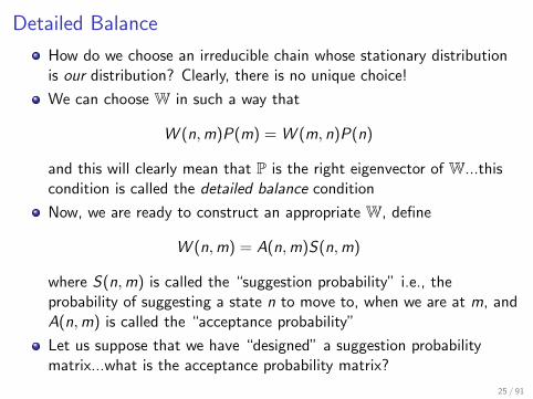
How do we choose an irreducible chain whose stationary distributionis our distribution? Clearly, there is no unique choice!

We can choose W in such a way that

W (n,m)P(m) = W (m, n)P(n)

and this will clearly mean that P is the right eigenvector of W...thiscondition is called the detailed balance condition

Now, we are ready to construct an appropriate W, define

W (n,m) = A(n,m)S(n,m)

where S(n,m) is called the “suggestion probability” i.e., theprobability of suggesting a state n to move to, when we are at m, andA(n,m) is called the “acceptance probability”

Let us suppose that we have “designed” a suggestion probabilitymatrix...what is the acceptance probability matrix?

25 / 91

Acceptance Matrix

We can use detailed balance and immediately the following equationfor the acceptance matrix

A(n,m)

A(m, n)=

S(m, n)P(n)

S(n,m)P(m)=

S(m, n)|Ψ(n)|2S(n,m)|Ψ(m)|2 ≡ h(n,m)

note that denominators are gone!

We now posit A(n,m) to be function of h(n,m), i.e.,

A(n,m) = F (h(n,m))

The first condition can be satisfied if the function F satisfies

F (y) = yF (1/y)

We have lots of freedom...we can choose any function that satisfiesthe above condition!

26 / 91

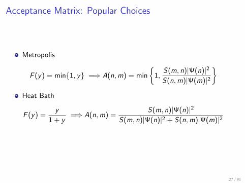
Acceptance Matrix: Popular Choices

Metropolis

F (y) = min{1, y} =⇒ A(n,m) = min

{

1,S(m, n)|Ψ(n)|2S(n,m)|Ψ(m)|2

}

Heat Bath

F (y) =y

1 + y=⇒ A(n,m) =

S(m, n)|Ψ(n)|2S(m, n)|Ψ(n)|2 + S(n,m)|Ψ(m)|2

27 / 91

Suggestion Matrix

Simplest suggestion matrix: Based on single electron moves

Single electron moves: Successive configurations differ only in theposition of a single electron

◮ At any step pick an electron at random◮ Move the electron from its current position to a new position also

picked at random◮ We have

S(n,m) =1

Nelectrons × (Nsites − 1)

Note that S(m, n) = S(n,m)

Metropolis acceptance matrix becomes

min

{

1,|Ψ(n)|2|Ψ(m)|2

}

...we have constructed our Markov matrix W Question: Does our W

produces an irreducible chain?

28 / 91

..and some Final Touches

We now generate a sequence of configurations mk starting from somerandom initial configuration using our Markov matrix W...say we takeNMC steps

The key result of importance sampling

E (αi ) =1

NMC

NMC∑

k=1

HΨα(mk)

Ψα(mk)

...and this work for other operators as well

〈O〉α =1

NMC

NMC∑

k=1

OΨα(mk)

Ψα(mk)

29 / 91

Variational Monte Carlo

VMC Summary

1 Start with a random configuration2 For k = 0,NMC

◮ In configuration mk , pick an electron at random, suggest a randomnew position for this electron, call this configuration m′

k

◮ Accept m′k as mk+1 with probability min

{

1,|Ψ(m′

k )|2

|Ψ(mk )|2

}

, if m′k is not

accepted, set mk+1 = mk

◮ Accumulate OΨα(mk+1)Ψα(mk+1)

3 Calculate necessary averages for E (αi )

4 Optimize over αi , obtain |ΨG 〉5 Study |ΨG 〉

30 / 91

Comments on VMC

Note that our starting configuration in most practical situations issampled from a different probability distribution from the one we areinterested in!

If we take sufficiently large number of steps we are guaranteed by thefundamental theorem that we will “reach” our desired distribution

How fast we attain our desired distribution depends next largesteigenvalue of W...it might therefore be desirable to design W suchthat all other eigenvalues of W are much less than unity

Passing remark: In VMC we know which P we want and we construct

a W to sample P...In “Green’s Function Monte Carlo” (GFMC) wehave a W = e−H , we start with some P(≡ |Ψ〉) and project out theground state PGroundState(≡ |ΨG 〉) by repeated application of W

31 / 91

VMC Computational Hardness

How hard is VMC?

For every step, once we make a suggestion for a new configuration,

we need to evaluate the ratio|Ψ(m′

k)|2

|Ψ(mk )|2

Now Ψ is usually obtained in a determinental form. If there are 2Nelectrons, we usually have determinants of order N × N

How hard is the calculation of a determinant? This is an N3 process...

Not too good, particularly since we have to optimize with respect toαi ...we like things to be O(N) hard!

...

...all is not lost!

32 / 91

Faster VMC

Note that throughout our calculation, we need only the ratio ofdeterminants, not the determinants themselves

To illustrate the idea behind this, consider spinless fermions; we havea configuration m given by a wavefunction |Ψ〉 and a configuration ngiven by a wavefunction |Φ〉 which differ by the position of a singleelectron l, rl and r ′l ; written in terms of matrices

[Ψ] =

ψa1(r1) · · · ψa1

(rl ) · · · ψa1(rN)

... · · ·...

...ψaN

(r1) · · · ψaN(rl) · · · ψaN

(rN)

and

[Φ] =

ψa1(r1) · · · ψa1

(r ′l ) · · · ψa1(rN)

... · · ·...

...ψaN

(r1) · · · ψaN(r ′l ) · · · ψaN

(rN)

where ψaiare some one particle states (which usually depend on αi )

33 / 91

Faster VMC

We need det[Φ]det[Ψ] ...key point:[Φ] and [Ψ] differ only in one column!

Now∑

k

Φ−1ik Φkj = δij =⇒

∑

k

CofΦkiΦkj = det[Φ]δij

=⇒∑

k

CofΦklΦkl = det[Φ]

CofΦkl = CofΨkl =⇒ det[Φ] =∑

k

CofΨklΦkl

=⇒ det[Φ]

det[Ψ]=

∑

k

Ψ−1kl Φkl

which is certainly O(N)

Note that we need to know Ψ−1, and thus have to store it at everystep!

When we accept a suggested configuration, we will have torecalculate Ψ−1 which, again, appears to be O(N3)!

34 / 91

Fast Update of Ψ−1 (Sherman-Morrison-Woodbury)

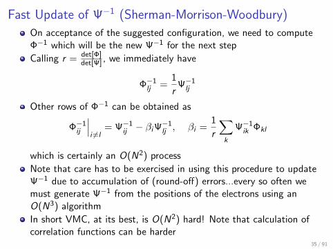
On acceptance of the suggested configuration, we need to computeΦ−1 which will be the new Ψ−1 for the next step

Calling r = det[Φ]det[Ψ] , we immediately have

Φ−1lj =

1

rΨ−1

lj

Other rows of Φ−1 can be obtained as

Φ−1ij

∣∣∣i 6=l

= Ψ−1ij − βiΨ

−1lj , βi =

1

r

∑

k

Ψ−1ik Φkl

which is certainly an O(N2) process

Note that care has to be exercised in using this procedure to updateΨ−1 due to accumulation of (round-off) errors...every so often wemust generate Ψ−1 from the positions of the electrons using anO(N3) algorithm

In short VMC, at its best, is O(N2) hard! Note that calculation ofcorrelation functions can be harder

35 / 91

Variational Monte Carlo

VMC Summary

1 Start with a random configuration2 For k = 0,NMC

◮ In configuration mk , pick an electron at random, suggest a randomnew position for this electron, call this configuration m′

k

◮ Accept m′k as mk+1 with probability min

{

1,|Ψ(m′

k )|2

|Ψ(mk )|2

}

, if m′k is not

accepted, set mk+1 = mk

◮ Update Ψ−1 if mk+1 = m′k using SMH formula (check every so often

and perform a full update)◮ Accumulate OΨα(mk+1)

Ψα(mk+1)

3 Calculate necessary averages for E (αi )

4 Optimize over αi , obtain |ΨG 〉5 Study |ΨG 〉

36 / 91

Free VMC Code pedestrianVMC

37 / 91

pedestrianVMC Examples

We will work on the square lattice, us-ing a tilted configuration, number of sites go as L2+1 (L has to be odd)

(Paramekanti, Randeria and Trivedi, PRB (2004))

Hubbard model

−∑

〈ij〉tijc

†iσcjσ + U

∑

i

ni↑ni↓

we will consider two cases: U = 0 (free electrons) and U =∞Number of electrons in the lattice is characterized by x the dopingfrom the half filled state (one electron for each lattice site

38 / 91

Free Gas (U = 0)

Guess for the ground state |Ψ〉 = |FS〉Suggestion matrix using single electon moves

x (hole doping)

Ene

rgy

per

site

0 0.1 0.2 0.3 0.4

-1.6

-1.55

-1.5

-1.45

Exact

MC

L = 9, NMC = 4000

...note we have sampled only 10−55 of the possible configurations!

39 / 91

Extremely Correlated Liquid (U =∞)

Guess |Ψ〉 = P|FS〉 – Projected Fermi Liquid...In terms of real spacewavefunctions the P means this: ∀ configurations C with at least onedoubly occupied site the wave function Ψ(C ) vanishes...doubleoccupancy is strictly forbidden

Suggestion matrix using single electon moves ...does NOT work! Needto introduce spin flip moves ... this is actually a two-electron move

x (hole doping)

Ene

rgy

per

site

0 0.1 0.2 0.3 0.4

-1.5

-1

-0.5

0

Free

Projected

L = 9, NMC = 16000

40 / 91

How well are we doing?

Sampling Error

Systematic Error (Random number generator etc.)

Finite Size Effects

...

Bugs

41 / 91

How well are we doing?

We use the estimator

〈O〉 =1

NMC

∑

k

Ok , Ok ≡OΨ(mk)

Ψ(mk)

for the expectation value of the operator

-0.1

0

0.1

0.2

0.3

0.4

0.5

0.6

0 500 1000 1500 2000 2500 3000 3500 4000 4500 5000

Ene

rgy

per

site

Monte Carlo Sweeps

We are sampling a finite chain... leads to sampling error

42 / 91

Sampling Error

Suppose we have a Gaussian distribution, want to find its mean valueby sampling...if we perform N independent samplings, we canestimate the mean with a standard error of σ/

√N where σ is the

variance of the Gaussian

In our case we can estimate the error as

ε2O =

⟨(

1

NMC

∑

k

Ok

)2⟩

−⟨

1

NMC

∑

k

Ok

⟩2

=1

N2MC

∑

jk

〈(Oj − 〈O〉)(Ok − 〈O〉)〉

=1

NMC

(∑

k

〈(Ok − 〈O〉)2〉)

+1

N2MC

∑

j 6=k

〈(Oj − 〈O〉)(Ok − 〈O〉)〉

=1

NMC

(σO)2 +1

NMC

NMC∑

k=1

(1− k

NMC

)λOk

43 / 91

Sampling Error

Autocorrelation function

λOk = 〈(Ok − 〈O〉)(O0 − 〈O〉)〉

clearly, σO =√

λO0

We see in addition to the variance, the auto correlation function alsocontributes to the errors

Always look at auto-correlation functions

k (MC sweep)

λ k/λ0

0 5 10 15 20

0

0.25

0.5

0.75

1

U = ∞, x = 0.1, L = 9

Not bad!44 / 91

Sampling Error: Blocking

There is a nice trick to calculate the error of auto-correlated datawithout calculating autocorrelations...this is calledblocking...attributed to Wilson

The idea is same as Kadanoff’ block spin RG trick... Start with thedata of size NMC which for convenience we can take to be a power of2, calculate its standard error ε0

Now generate new data which is of size NMC/2 byOblocked

k = (O2k + O2k+1)/2 and calculate its standard error ε1...thesubscript “1” stands for first level of blocking

Continue this procedure (you need sufficient data) and plot εb as afunction b where b is the number of block transformations applied

Pick the plateau value for the error

45 / 91

Sampling Error: BlockingOur example, we are doing okay

Number of blocks

Stan

dard

Err

or

0 2 4 6 8 10

1.0x10-04

1.5x10-04

2.0x10-04

2.5x10-04

3.0x10-04

3.5x10-04

4.0x10-04

U = ∞, x = 0.1, L = 9, NMC = 215

An example with strong auto-correlations

(Flyvbjerg and Petersen, JCP (1984))

46 / 91

Equilibration

Howto check for equilibration...run calculations with different random seeds!

nmc (Number of Monte Carlo Sweeps)

Ene

rgy

per

site

103 104 105

-0.257

-0.256

-0.255

-0.254

-0.253

Colours stand for different random seeds

U = ∞, x = 0.1, L = 9

“Large” seed-dependence is a sure sign of non-equilibration...we aredoing okay when NMC ≥ 10000 in this example

47 / 91

One Final Check

How well can we do?If everything is okay the error should fall of as 1/

√NMC

Nmc

ε

103 104 105

5.0x10-04

1.0x10-03

U = ∞, x = 0.1, L = 9

We are doing pretty okay!...But, are we really?

48 / 91

Another Difficulty

When we want to optimize with respect to the variational parameters,we will have to evaluate the energy many times over...long thatreduce error bars are prohibitive

Shorter runs produce data that are bumpy, and seed dependent...

The problem is particularly severe if the minimum is “shallow”...andbecomes worse with increasing number of variational parameters

49 / 91

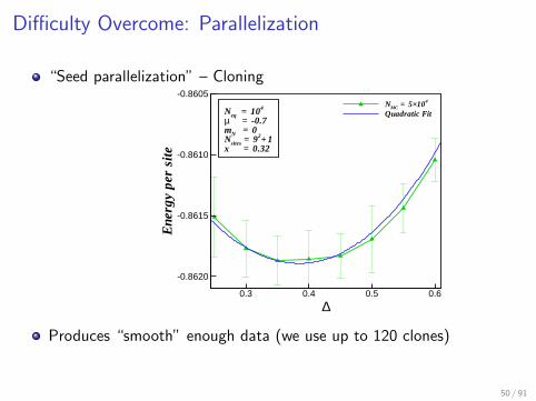
Difficulty Overcome: Parallelization

“Seed parallelization” – Cloning

∆

Ene

rgy

pe

rsi

te

0.3 0.4 0.5 0.6

-0.8620

-0.8615

-0.8610

-0.8605NMC = 5×104

Quadratic FitNeq = 104

µ = -0.7mN = 0Nsites = 92+ 1x = 0.32

Produces “smooth” enough data (we use up to 120 clones)

50 / 91

Optimizing Variational Parameters

No derivative information◮ Direct search◮ Simplex method (use amoeba routine from Numerical Recipes)◮ Genetic algorithms?

Method with derivative information

51 / 91

Results of Force Method

Seed average forces

∆

Ene

rgy

pe

rsi

te

0.3 0.4 0.5 0.6

-0.8620

-0.8615

-0.8610

-0.8605NMC = 5×104

Quadratic FitNeq = 104

µ = -0.7mN = 0Nsites = 92+ 1x = 0.32

∆

dE

/d∆

0.3 0.4 0.5 0.6

-0.0100

-0.0050

0.0000

0.0050

NMC = 5×104

Forces from quadratic fit to energyZero reference

Neq = 104

µ = -0.7mN = 0Nsites = 92+ 1x = 0.32

Results for optimized variational parameters

52 / 91

Variational Monte Carlo

VMC Summary

1 Start with a random configuration2 For k = 0,NMC

◮ In configuration mk , pick an electron at random, suggest a randomnew position for this electron, call this configuration m′

k

◮ Accept m′k as mk+1 with probability min

{

1,|Ψ(m′

k )|2

|Ψ(mk )|2

}

, if m′k is not

accepted, set mk+1 = mk

◮ Update Ψ−1 if mk+1 = m′k using SMH formula (check every so often

and perform a full update)◮ Accumulate OΨα(mk+1)

Ψα(mk+1)

3 Calculate necessary averages for E (αi )

4 Optimize over αi , obtain |ΨG 〉5 Study |ΨG 〉

Finally, our answers will be only as good as our guess...

53 / 91

Applications to Superconductivity: Overview

Essential High Tc

Models etc..

RVB Wavefunction + VMC Results

Material dependencies of the phase diagram

Graphene

54 / 91

References on VMC in High Tc

Gross et al., Giamarchi et al., Ogata et al., TKLee et al., PLee et al.and others

Paramekanti, Randeria, Trivedi, PRB (2004) (see also, earlier PRL)

(A2Z) Anderson, Lee, Randeria, Rice, Trivedi, Zhang, JPCM (2004)

Recent comprehensive review: Edegger, Muthukumar, Gros Adv.

Phys (2007)

55 / 91

Cuprate Phase Diagram

Generic phase diagram

(Damascelli et al. 2003)

Undoped system is a Mott insulator

Note the electron-hole asymmetry

56 / 91

Cuprates: Phase Diagram

Key features

d-Superconductor

“Strange” Metal

Pseudogap Phase

Antife

rrom

agnet

xAF x

T

?

xo

Tmaxc

xAF – doping at which AF dies

Tmaxc – maximum superconducting Tc

xo – optimal doping

57 / 91

Model Hamiltonian

What is the minimal model?

One band model (Anderson et al.)

Undoped system is a Mott insulator...must have large onsite repulsion

Minimal model - one band Hubbard model

HH = −∑

〈ij〉tij(c

†iσcjσ + h.c .)− µ

∑

iσ

niσ

︸ ︷︷ ︸

K

+U∑

i

ni↑ni↓

Related tJ model

HtJ = P −∑

〈ij〉tij(c

†iσcjσ + h.c .)P − µ

∑

iσ

niσ

+ J∑

〈ij〉

(

Si · Sj −1

4ninj

)

︸ ︷︷ ︸

HJ

P stands for projection – hopping should not produce doublons

58 / 91

Are the two Models Related?

Apply a canonical transformation on the Hubbard model to “projectout” doubly occupied sector of the Hilbert space

Canonical transformation e iSHe−iS ...this leads to

PHHP = PKP + HJ + HK3site︸ ︷︷ ︸

O(t2/U)

J is now related to t and U as

J =4t2

U

can be understood from a two site model

Typically U ∼ 10− 12t, J/t ∼ 0.3, t ∼ 0.3− 0.5eV

Note that U →∞ gives us

HU=∞ = PKP

which we had seen earlier59 / 91

U =∞ Revisited

Nothing can hop at half filling...what happens at a doping x?

Ask the question: What is the relative probability an electron will finda hole on the neighbouring site?...this can be shown to be gt = 2x

1+x

Suggests that

H = PKP 7→ gtK !

which is now a “free particle” Hamiltonian!

How well does this do?

60 / 91

U =∞ Revisited

Our guess for the ground state is |Ψ〉 = P|FS〉...The “projected kinetic energy” is 〈Ψ|H|Ψ〉 = gt〈FS |K |FS〉

x (hole doping)

Ene

rgy

per

site

0 0.1 0.2 0.3 0.4

-1.5

-1

-0.5

0

gt × Free

Projected

Free

L = 9

Does okay?...looks like!

61 / 91

U =∞ and the tJ model

From the U =∞ results, we see immediately that kinetic energy isbadly “frustrated”

What happens when we add the HJ to PKP?...this is the tJ model

At zero doping (x = 0) we get

HtJ =︸︷︷︸

x=0

J∑

〈ij〉Si · Sj

which is the Heisenberg model...

On a square lattice we know this has a Neel ground state (with asmaller staggered magnetization)

62 / 91

tJ model...effect of doping

Projection badly frustrates kinetic energy...what is the effect of HJ onkinetic energy?

Hj wants singlets...but this is “localizing” and frustrates the kineticenergy further...

Expect◮ J to win over t at “small” doping...very little kinetic energy to be

gained...lots of J energy to gained◮ At “large” doping expect kinetic energy to win◮ Doping where competition is most severe 2xt ∼ J =⇒ x ∼ 0.15!!

Who wins?

63 / 91

Ground State at Finite Doping

Actually, both, in a superconducting state!

Both J and t can be satisfied by forming resonating singlets Ideaembodied in the Resonating Valance Bond (RVB) state, Anderson(1987)

How do we construct an RVB state?

Will (can) it be a superconductor of the right pairing symmetry?

64 / 91

Mean Field Theory

Keep projection aside...rewrite the tJ Hamiltonian as

HtJ = K − J∑

ij

b†ijbij

where b†ij ∼ (c†i↑c

†j↓ − c

†i↓c

†j↑)

Construct a meanfield Hamiltonian

HMF = K −∑

ij

∆ijbij + ...

where ∆ij ∼ J〈b†ij〉... is the “singlet pair amplitude”

Translational invariance two pair amplitudes ∆x and ∆y — d

symmetry is obtained by keeping ∆x = ∆ and ∆y = −∆

We now have a BCS like Hamiltonian, ground state

|dBCS〉 =∏

k

(uk + vkc†k↑c

†−k↓)|0〉

65 / 91

dRVB state

The “guess” for the ground state is

|Ψ〉 = P|dBCS〉 = eP

k φkc†k↑c

†−k↓ |0〉 φk =

vk

uk

For working on a lattice

|Ψ〉 = P

(∑

k

φkc†k↑c

†−k↓

)N/2

|0〉

= P

(∑

k

φ(i − j)c†i↑c†j↓

)N/2

|0〉

All our variational parameters are buried in φ(i − j), the “pairwavefunction”

66 / 91

Variational Wavefunction

Given variational parameters construct φ

Pick number of electrons N using doping x = 1− NNL

(NL number ofsites)

Variational wave function

PΨ({ri↑, rj↓}) =

∣∣∣∣∣∣∣

φ(r1↑ − r1↓) . . . φ(r1↑ − rN/2↓)...

. . ....

φ(rN/2↑ − r1↓) . . . φ(rN/2↑ − rN/2↓)

∣∣∣∣∣∣∣

Optimize, obtain the ground state, and study it

67 / 91

Superconducting order parameter

The superconducting correlation function

Fα,β(r − r′) = 〈b†

rαbr′β〉

b†rα = 1

2(c†r↑c

†r+α↓ − c

†r↓c

†r+α↑) creates a singlet on the bond (r, r + α),

α = x , y

SC order parameter

Φ = lim|r−r′|−→∞

Fα,α(r − r′)

Off-diagonal Long Range Order (ODLRO)

68 / 91

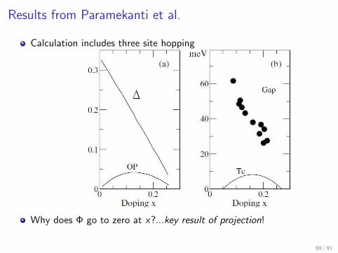
Results from Paramekanti et al.

Calculation includes three site hopping

Why does Φ go to zero at x?...key result of projection!

69 / 91

More results from Paramekanti et al.

Seems to agree qualitatively with many experiments

What about antiferromagnetism?

70 / 91

Cuprates: Our Focus

Is there a transition from antiferromagnetic ground state to asuperconducting state? What is the nature of this transition? Doantiferromagnetism and superconductivity co-exist? (Previous work:

Gros et al, 1988, Giamarchi et al 1990, Ogata et al, 1995, Lee et al. 1995-2003)

What is the origin of the electron-hole asymmetry? Why doeselectron doping ”protect” the antiferromagnetic state?

What energy scales determine the answers to the above questions?Does the next-near neighbour and third-near neighbour hopping affectthe ground state and the transition? How?

There is a suggestion (Pavarini et al., PRL, 2001)) based on the results offirst principles calculations that Tmax

c is correlated with the ratio ofthe second neighbour hopping to that of the nearest neighbourhopping? What is the microscopic reason behind this?

Is there a “single parameter” description of the phase diagram thatcaptures the “material dependencies”?

71 / 91

Material Dependence of Tmaxc

Range parameter r = t ′/t, t ′′ = t ′/2 (Pavarini et al., 2001)

Correlation between Tmaxc and r , r obtained from ab initio electronic

structure methods

72 / 91

Meanfield Theory

Meanfield breakup up of Si · Sj =“

c†iα

12σαβciβ

”

·“

c†jα′

12σα′β′cjβ′

”

Neel channel

Si · Sj ∼ 〈Si 〉Sj + ...

with 〈Si 〉 = mNezeiRi ·Q,Q = (π, π)

d-wave channel

Si · Sj ∼ ∆ij

“

c†i↑c

†j↓ − c

†i↓c

†j↑

”

+ ...

with ∆ij = ∆ on x-bonds and ∆ij = −∆ on y -bonds

“Fock”-channel

Si · Sj ∼ χijc†iσcjσ + ...

with χij = χ′, χ′′ ... “renormalizes” kinetic energy

Four “molecular field parameters”: mN , ∆, χ′, χ′′

73 / 91

Meanfield Theory

Mean field Hamiltonian

HMF =X

k,σ

ξ(k)c†kσckσ

+1

2

X

k

∆(k)“

c†k↑c

†−k↓ + h. c.

”

+1

2

X

kσ

σmNJ(Q)c†

k+Q,σckσ

contains five parameters {χ′, χ′′,∆,mN , µ} – gives the “one particle”states

∆: Gap parameter

mN : Neel order parameter

µ: Hartree shift

χ′, χ′′ : Fock shifts

74 / 91

Variational Ground State Construction

Constructed in two steps◮ Diagonalize the Hamiltonian without the paring term...give rises to two

SDW bands d†kα

which disperse as Eα(k)◮ Introduce pairing in the two spin split bands...no “cross pairing” terms

ariseConstruct a BCS wavefunction

|Ψ〉 =Y

kα

(ukα + vkαd†kα↑

d†−kα↓

)|0〉,vkα

ukα

= (−1)α−1 ∆(k)

Eα(k) +q

E2α(k) + ∆2(k)

, α = 1, 2

Project to N particle subspace

|Ψ〉N =

0

@

X

i,j

ϕ(Ri↑, Rj↓)c†i↑

c†j↓

1

A

N/2

|0〉

The “pairing function” ϕ(Ri ,Rj) is determined by the parametersmN ,∆...

75 / 91

Electron Doping

Electron doped Hamiltonian is obtained by a particle-holetransformation (Lee et al. 1997, 2003, 2004)

c† −→ c on A sublattice, c† −→ −c on B sublattice

Corresponds to t −→ t, t ′ −→ −t ′, t ′′ −→ −t ′′

Choose sign convention such that holed doped side has all tspositive...electron doped side will have t ′ and t ′′ negative...

76 / 91

What do we measure?

Staggered magnetization

M =2

N〈∑

i ǫA

Szi −

∑

i ǫB

Szi 〉

The superconducting correlation function (Paramekanti et al. 2004)

Fα,β(r − r′) = 〈B†

rαBr′β〉

B†rα = 1

2(c†r↑c

†r+α↓ − c

†r↓c

†r+α↑) creates a singlet on the bond (r, r + α),

α = x , y

SC order parameter

Φ = lim|r−r′|−→∞

Fα,α(r − r′)

Off-diagonal Long Range Order (ODLRO)

77 / 91

Phase Diagram (t ′′ = 0)

Electron Doping, x

OD

LRO

,Φ(×

10-4

)

00.10.20.30.40

20

40

60

80

100

t’’/t = 0.0, J/t = 0.3

t’ < 0

MΦ

Hole Doping, x

M

OD

LRO

,Φ(×

10-4

)

0.1 0.2 0.3 0.4 0.5

0.4

0.8

20

40

60

80

100

t’ > 0

,

t’ = 0.3

t’ = 0.0

t’ = 0.1 t’ = 0.2

,,,

SC and AF coexist on both h and e doped systems

With increasing |t ′|, SC enhanced on h doped side, AF on the e

doped side ((Lee et al, 2004, Trambley et al, 2006, Kotliar et al 2007))

New result: |t ′| does not affect xAF on the hole doped side, andslightly “weakens” SC on the e doped side

78 / 91

Phase Diagram (t ′′ 6= 0)

Hole Doping, x

M

OD

LRO

,Φ(×

10-4

)

0 0.1 0.2 0.3 0.4 0.5

0.2

0.4

0.6

0.8

0

20

40

60

80

100

t’/t = 0.3

, t’’ = 0.15

, t’’ = 0.00, t’’ = 0.03, t’’ = 0.06, t’’ = 0.12

t’’ > 0

Electron Doping, x

OD

LRO

,Φ(×

10-4

)

00.10.20.30.40

20

40

60

80

100

t’/t = -0.3, J/t = 0.3

t’’ < 0

MΦ

h-doped: Increasing |t ′′| enhances SC, xAF is unaffected

e-doped: Increasing |t ′′| enhances AF, SC is unaffected

...

Is there a “single parameter” characterization...a unified picture?

79 / 91

Fermi Surface Convexity Parameter η

kx/πk y/

π-0.5 0 0.5 1

-0.5

0

0.5

1

θkF

kx/π

k y/π

-0.5 0 0.5 1

-0.5

0

0.5

1

Bare Fermi surface (BFS) at zero doping

Fermi surface convexity parameter

η = 2

(k NODEF

kANTINODEF

)2

η = 1 when t ′ = t ′′ = 0

η > 1 convex BFS, η < 1 concave BFS

Claim: “Everything” is determined by η (for given t and J); ConvexBFS encourages AF, concave BFS promotes SC!

80 / 91

Fermi Surface Convexity Parameter η

t’/t

t’’/t

-0.50 0.00 0.50-0.50

0.00

0.50

3.6

3.0

2.4

1.8

1.2

0.6

ηt’’= t’/2

t’/t

η

-0.50 0.00 0.50

1.0

2.0

3.0

4.0t’’ = t’/2

η > 1 convex BFS, η < 1 concave BFS

For t ′′ = t ′/2: η is monotonically related to range parameter ofPavarini et al.!

Valid for t ′′ 6= t ′/2

81 / 91

“Extent” of antiferromagnetism xAF and η

η

AF

ext

ent

,xA

F

0.5 1.0 1.5 2.0 2.5

0.10

0.15

0.20

0.25

0.30Electron DopingHole Doping

t’= 0.0, t’’= 0.00t’= -0.3, t’’= 0.15

t’= 0.3, t’’= 0.06t’= 0.4, t’’= 0.00

Convex BFS promote AF, xAF increases linearly with η!

Different values of t ′, t ′′ with same η fall on top of each other!

82 / 91

Optimal ODLRO Φmax and η

η

Φm

ax(×

10-4

)

0.5 1.0 1.5 2.0 2.5

10

20

30

40

50Electron DopingHole Doping

η

Tc

ma

x

0.55 0.6 0.65 0.7 0.75 0.8 0.85

20

40

60

80

100

120

140

YBa2Cu3O7

HgBa2Ca2Cu3O8

HgBa2CaCu2O6Tl2Ba2Ca2Cu3O10

LaBa2Cu3O7

HgBa2CuO4

La2CaCu2O6

TlBaLaCuO5

Bi2Sr2CuO6

La2CuO4d

Pb2Sr2Cu2O6Ca2CuO2Cl2

Tl2Ba2CuO6

The maximum ODLRO (Φmax) is promoted by a concave BFS

Φmax taken to be a measure of Tc , suggests η “determines” Tc !

Consistent with experiments, Pavarini et al., 2001

83 / 91

Physics of η

Key (well known) point: t ′ and t ′′ do not disturb the AF background

Question: Do t ′, t ′′ help gain kinetic energy?

84 / 91

Physics of η

Not always! Look at the bare kinetic energy as fn. of doping

Doping

Ba

reki

netic

ene

rgy

pe

rsi

te

0.0 0.1 0.2 0.3 0.4-2.0

-1.8

-1.6

-1.4

-1.2

-1.0η = 3.0η = 2.0η = 1.0η = 0.7η = 0.6

xmxm

Concave FS

Convex FS

For η > 1, the bare KE falls with increasing doping, attains aminimum at xBKE

m

xBKEm increases with η

This gain in KE arises from t ′, t ′′ and hence AF will be stable untilxBKEm ...explains why xAF increases with η!

85 / 91

Physics of η

Doping

Ba

reki

netic

ene

rgy

pe

rsi

te

0.0 0.1 0.2 0.3 0.4-2.0

-1.8

-1.6

-1.4

-1.2

-1.0η = 3.0η = 2.0η = 1.0η = 0.7η = 0.6

xmxm

Concave FS

Convex FS

For η < 1, the bare KE monotonically increases with doping...greaterrate of increase of BKE for more concave FS...

Plausible that SC is stabilized in this case...both KE and exchangeenergies are happy!

86 / 91

Summary

What is done

VMC of t − t ′ − t ′′ − J model...a detailed study of materialdependencies

An efficient method for optimizing variational wavefunctions

What is learnt

Cuprate phase diagram is characterized by a single parameter...η (forgiven t and J)

Difference between hole and electron doping

Microscopic origin of Pavarini et al. relation

Suggestion to increase Tc : Make BFS more concave!

Reference

S. Pathak, V. B. Shenoy, M. Randeria, N. Trivedi, Phys. Rev. Lett. 102,027002 (2009)

87 / 91

Graphene: Superconductor?

Work done in collaboration with G. Baskaran

Graphene - many benzene’s connected togather

Pauling’s idea of resonance

Graphene: Correlated or not?

Experiments suggest a U/t ∼ 2.4

Not strongly correlated

88 / 91

Graphene Superconductivity

Singlet formation tendency...J (difference between singlet tripletenergies)

Undoped graphene has zero density of states...MFT suggests that acritical J is required to induce SC

J in graphene is lower than the critical value, undoped graphene isnot a SC

What about doped graphene?

Meanfield theory of Black-Schaffer suggested a d + id state

89 / 91

Graphene Superconductivity: VMC Results

|Ψ〉 = gD |BCSd+id〉

Doping, x

SC

Ord

er

Pa

ram

ete

r,Φ(×

10-4

)

0 0.1 0.2 0.30

2

4

6

Distance, r

SC

Co

rre

latio

nfu

nctio

n,F

(r)

2 3 4 5 6 70

5

10

15

20

25

Optimum doping around x ∼ 0.15

Agrees with other works e.g., Honerkamp, PRL (2008)

90 / 91