Embed Size (px)
Citation preview

Variational Constitutive Updates for Strain
Gradient Isotropic Plasticity
by
Lei Qiao
B.S., Mathematics (2004)M.S., Mathematics (2007)
Peking University
MASSACHUSETT EOF TECHNOLOGY
SEP 2 2 2009
LIBRARIES
Submitted to the School of Engineeringin Partial Fulfillment of the Requirements for the Degree of
Master of Science in Computation for Design and Optimization
at the
MASSACHUSETTS INSTITUTE OF TECHNOLOGY
September 2009
@ Massachusetts Institute of Technology 2009. All rights reserved.
ARCHIVES
A uthor ..................... .....................................School of Engineering
SAugust 52009
Certified by............... . . . . . . . . . .. . . . . . . . . . . . . . . . .. .."- Rail A. ljdovitzky
Accepted by..
Associate Professor of Aeronautics and Astronautics
1 I pT~esis Supervisor
Jaime PeraireProfessor of Aeronautics and Astronautics
Director, Computation for Design and Optimization Program


Variational Constitutive Updates for Strain Gradient
Isotropic Plasticity
by
Lei Qiao
Submitted to the School of Engineeringon August 5, 2009, in partial fulfillment of the
requirements for the Degree ofMaster of Science in Computation for Design and Optimization
Abstract
In the past decades, various strain gradient isotropic plasticity theories have beendeveloped to describe the size-dependence plastic deformation mechanisms observedexperimentally in micron-indentation, torsion, bending and thin-film bulge tests inmetallic materials. Strain gradient plasticity theories also constitute a convenientdevice to introduce ellipticity in the differential equations governing plastic deforma-tion in the presence of softening. The main challenge to the numerical formulationsis that the effective plastic strain, a local internal variable in the classic isotropicplasticity theory, is now governed by the partial differential equation which includesspatial derivatives. Most of the current numerical formulations are based on Aifantis'one-parameter model with a Laplacian term [Aifantis and Muhlhaus, ijss, 28:845-857,1991]. As indicated in the paper [Fleck and Hutchinson, jmps, 49:2245-2271, 2001],one parameter is not sufficient to match the experimental data. Therefore a robustand efficient computational framework that can deal with more parameters is still inneed.
In this thesis, a numerical formulation based on the framework of variational con-stitutive updates is presented to solve the initial boundary value problem in straingradient isotropic plasticity. One advantage of this approach compared to the mixedmethods is that it avoids the need to solve for both the displacement and the ef-fective plastic strain fields simultaneously. Another advantage of this approach is,as has been amply established for many other material models, that the solutionof the problem follows a minimum principle, thus providing a convenient basis forerror estimation and adaptive remeshing. The advantages of the framework of vari-ational constitutive updates have already been verified in a wide class of materialmodels including visco-elasticity, visco-plasticity, crystal plasticity and soil, howeverthis approach has not been implemented in the strain gradient plasticity models. Inthis thesis, a three-parameter strain gradient isotropic plasticity model is formulatedwithin the variational framework, which is then taken as a basis for finite elementdiscretization. The resulting model is implemented in a computer code and exer-cised on the benchmark problems to demonstrate the robustness and versatility of

the proposed method.
Thesis Supervisor: Raiil A. RadovitzkyTitle: Associate Professor of Aeronautics and Astronautics

Acknowledgments
I would like to thank my advisor Prof. Ra61l Radovitzky. His guidance and support
have been making my study at MIT progress very smoothly in the last two years.
Without his counsel, I would not have been able to get into this interesting and active
research field.
I am grateful to the director of the CDO program, Prof. Jaime Peraire, who
launched this exciting interdepartmental program at MIT.
I am thankful for the help of the administrator of the CDO program, Laura Koller.
Her patience and her kind emails allow me, a 'trouble maker', to survive all the paper
work.
I would like to thank the assistants of our group, Brian, Ed and Melanie. Their
work enables me to not worry about the administrative affairs.
I am grateful to Dr. Ludovic Noels for his nice introduction of both the dG method
and the variational constitutive updates.
I should express my appreciation to the group members, Antoine, Tan, Ganesh,
Michelle, Rupa, Andy, Mike, Brandon and Li. I am very lucky and happy to work
with them, and enjoy the lunches and parties together.
Finally, great thanks to my parents and family, my girl friend, Yan, and also to
my friends here, Minglin and Henry. Their encouragement is not only important but
also indispensable to my study and life.


Contents
1 Introduction 13
2 Strain gradient models of plasticity 19
3 Numerical methods for strain gradient isotropic plasticity 33
3.1 Summary of current numerical methods . ................ 33
3.2 Variational constitutive updates applied to Fleck and Hutchinson's model 35
3.3 Finite element formulation . .................. ..... 40
3.3.1 Computational framework . .................. . 41
3.3.2 Derivation of main equations . .................. 42
4 Numerical examples 49
4.1 Shearing of a layer sandwiched by two rigid substrates ........ 51
4.2 Wire torsion ................ ...... ........ 60
5 Discussion and conclusions 71
5.1 Fleck and Hutchinson's model revisited . ................ 71
5.2 Other problems with coupled fields . .................. 74
5.2.1 Gradient damage model ................... .. 75
5.3 Conclusions ................. . ............ 76
A 79
A.1 Expression of the generalized effective plastic strain rate ....... 79
A.2 Proof of the minimum principle ................... .. 81
A.3 Derivation of the optimality conditions . .............. . 87

List of Figures
Sandwich layer: illustration . . . . . . . . . . . . . ..
Sandwich layer: distribution of the displacement . . .
Sandwich layer: distribution of the plastic strain . . . .
Sandwich layer: distribution of the shear stress . . . . .
Sandwich layer: distribution of the generalized effective
Sandwich layer: evolution of the shear stress . . . . . .
Sandwich layer: effect of the boundary conditions . . .
Sandwich layer: convergence of the plastic shear strain
Sandwich layer: convergence of the displacement . . ..
Wire torsion: distribution of the plastic shear strain . .
Wire torsion: torque v.s. twist ..............
Wire torsion: distribution of the plastic shear strain . .
Wire torsion: zoom-in of Fig (4-12) . . . . . . . ....
.. . . . . . 50
. . . . . . . . 53
. . . . . . . . 54
. . . . . . . . 55
plastic strain 56
. . . . . . . . 58
. . . . . . . . 59
. . . . . . . . 60
. . . . . . . . 61
. . . . . . . . 65
.. . . . 66
. . . . . . . . 67
.. . . . . 68
4-1
4-2
4-3
4-4
4-5
4-6
4-7
4-8
4-9
4-10
4-11
4-12
4-13

10

List of Tables
2.1 List of variables .. ..... .............. .. . . . . . . 20
4.1 Material parameters -1 ................... ....... 52
4.2 Material parameters -2 .......... . . ... . ....... 63

12

Chapter 1
Introduction
Plastic deformation on the micron scale plays an important role in a number
of technological applications including micro-electronic-mechanical systems (MEMS)
and the structural materials, where the components' size as well as the deformation
are usually on this scale. Experiments reveal a prominent size-dependence effect for
plastic deformation on this scale. Examples of these experiments include the inden-
tation test [28], wire torsion [13], microbend [29] and thin-film bulge [32]. Basically,
this size-dependence effect can be stated as smaller is stronger. For example, in the
wire torsion test [13], the thinner the wire, the stronger the material response. Con-
ventional plasticity theories are unable to explain this effect, because no length scales
are considered.
There are different ways to model plastic deformation with size-dependence be-
havior. The choice of approaches depends on the interest. Dislocation dynamic and
molecular dynamic methods are useful to understand the basic physical mechanisms
such as the dislocation interactions [33]. Continuum descriptions are needed to de-
scribe the effective response and to solve initial boundary value problems, which will
be the focus of this thesis.
A number of continuum theories that account for the size-dependence effect in
plastic deformation have been proposed. Perhaps owing to their phenomenological
nature, there is no consensus on any specific theory. Apparently, the first higher
order gradient model can be attributed to Aifantis et al [3]. In order to remove

the plastic strain singularity in the presence of softening, they added higher order
gradient terms V 2EP and V4E in the conventional flow rule; e is the effective plastic
strain, and V2 is the usual Laplacian operator. Each new term introduces an internal
material length scale as a parameter, which is required by dimensional arguments.
These higher order gradient terms bring in the ellipticity to the governing partial
differential equations, and consequently eliminate the mesh dependence behavior that
appears in the simulation of the plastic flow in the softening regime. Motivated by the
size-dependence observed in wire torsion tests, Fleck and Hutchinson formulated a
strain gradient plasticity model based on the extensions of the couple stress theory and
Toupin-Mindlin theory. In their original model, the gradients of the total strains are
considered [11]. Later, they reformulated the model and eliminated the dependence
on the gradients of elastic strains because this dependence is not correct in the linear
elastic range [12]. Starting from the invariants of the plastic strain gradients VEP , a
third order tensor, they formulated a generalized effective plastic strain which includes
three internal material length scales [12]. Based on this generalized effective plastic
strain, Fleck and Hutchinson proposed a minimum principle for strain hardening
materials, from which the forces balance equations, the boundary conditions and the
evolution of the flow stress can be derived straightforwardly through variation. Both
Aifantis' model and Fleck and Hutchinson's model (FH mdoel) adopt the conventional
normality relation of the isotropic plasticity, i.e. the flow direction is collinear with
the deviatoric part of the Cauchy stresses. Regarding the requirement from thermo-
dynamics, some strain gradient plasticity models that do not obey the conventional
normality relation are also proposed. Gudmundson generalized the FH model in the
sense that the flow direction is collinear with the sum of the deviatoric Cauchy stress
tensor and the divergence of the moment stresses (or higher order stresses) which
are associated with the plastic strain gradient [16]. Similar to the FH model, three
internal material length scales appear in the expression of the generalized effective
plastic strain. In parallel to Gudmundson's work, Gurtin and Anand also considered
the thermo-dynamic requirement. They proposed a strain gradient plasticity model
that involves the back stress and accounts for the visco-plastic effect [17]. The flow

stress in their model is assumed to be a power function of the plastic strains and
plastic strain gradients. The aforementioned strain gradient plasticity models, with
the exception of the visco-plasticity model, have a commonality that the flow stress
rate depends linearly on the plastic strain gradient rate. In contrast, Nix and Gao
proposed a strain gradient plasticity model (NG model) where the square of the
flow stress has a linear dependence on the plastic strain gradient. They based this
relation on the analysis of the indentation experiments in [15, 19]. Recently, Evans
and Hutchinson assessed the NG model and FH model using the simple bending test
as an example [9]. They retained the variational framework of the FH model but
modified an exponent in the definition of the generalized effective plastic strain. The
resulting model demonstrates that the square of the flow stress depends linearly on
the plastic strain gradient as indicated by the NG model, and it also inherits the
flexible boundary conditions of the effective plastic strain from the FH model.
Regarding the formulation of numerical methods for strain gradient plasticity
models, the main distinction between the gradient and the classic or local models is
that the effective plastic strain in the gradient models can not be obtained locally,
since its governing partial differential equations include the spatial derivatives. In
addition, there is sometimes a need to distinguish the conditions for the boundaries
where the dislocations are free to pass by from the boundaries where dislocations
are stacked. Examples of the latter case can be found in the passivated layer test
in [32]. Popular numerical methods for the classic (or local) models, such as return
mapping method, fail to distinguish these two types of boundary conditions, since
the measurement of the dislocation density, the effective plastic strain, is not treated
as an independent variable.
The initial work on the numerical formulation for strain gradient plasticity should
be attributed to de Borst and Muhlhaus [5]. They presented a mixed formulation with
the displacement and the effective plastic strain treated as nodal unknowns to simulate
the strain softening behavior. In their formulation, Aifantis' one parameter model
with Laplacian term is used; the displacement and effective plastic strain fields are
updated simultaneously. The same treatment of these two fields was taken in [26, 8]

for different strain gradient plasticity models. The main benefit of this simultaneous
update is that no additional sensitivity analysis is required, while this treatment has
a deficiency that the linear algebraic system to be solved has a huge size. This seems
to not be a serious problem for isotropic plasticity, where there are only 4 unknowns
per node (3 for the displacement field and 1 for the effective plastic strain field).
In the crystal plasticity, however, there are many more unknowns. Take the FCC
material as an example. Generally, there are 15 unknowns per node, 3 of which are
the displacements and 12 of which are the plastic slips for the 12 slip systems. The
linear algebraic system built through the mixed formulation would become too huge
to be solvable with current computer systems. Apart from the mixed formulation,
some efforts have been made toward developing staggered methods [4, 6, 7]. In these
staggered methods, the solution is achieved through a two-level structure. The outer
level is the Newton-Raphson iteration for the displacement field and the inner level is
the stress update. Once a tentative displacement is obtained from the outer level, the
effective plastic strain is solved within the inner level and the stresses are updated
consequently. The main advantage of staggered methods is that the algebraic system
to be solved is divided into two sub-systems with much smaller sizes, while additional
cost of formulating the consistent tangential matrix for the outer level iteration is
inevitable. In particular, staggered methods require the sensitivity analysis of the
effective plastic strain P with respect to the displacement field u, i.e. estimating u,
which is not trivial due to the nonlocal effect.
In this thesis, a numerical formulation based on the framework of variational con-
stitutive updates is presented to solve the initial boundary value problem in strain
gradient isotropic plasticity. The framework of variational constitutive updates was
initially laid out by Radovitzky and Ortiz [25] for a wide class of material models,
and later applied to a wide variety of specific material phenomena including visco-
plasticity [24], viscoelasticity [10], porous elasto-plastic materials [30], soil [23] and
nonlinear solid dynamics [22]. The basic idea of variational constitutive updates is
that, within each increment in time, the value of internal state variables such as
the effective plastic strains can be consistently obtained through the variation of

an appropriate functional with respect to appropriate conjugate variables, given the
displacement or deformation gradient. Compared to other staggered methods, the
solution to the problem will follow from a minimum principle and the symmetry of
the consistent tangent matrix is guaranteed. Furthermore, the minimum principle
provides a convenient basis for error estimation and adaptive remeshing. The advan-
tages of the framework of variational constitutive updates have already been verified
for many material models, however, to the author's knowledge, it has not been im-
plemented on strain gradient plasticity theories. The numerical formulation to be
presented employs the FH model [12], which has a relatively simple form and is suf-
ficiently general. In addition, the minimum principle for the incremental version of
the FH model provides a solid foundation for variational constitutive updates.
The rest of this thesis is organized as follows. Chapter 2 serves as a brief overview
of strain gradient isotropic plasticity models, where only the FH model [12] will be
discussed in detail. In Chapter 3, the numerical formulation based on the framework
of variational constitutive updates will be presented. In Chapter 4, two numerical
examples, shearing of a layer sandwiched by two subtrates and wire torsion, are
provided to demonstrate the robustness and efficiency of this numerical formulation.
In Chapter 5, the recent improvements on the FH model, the extension of the proposed
numerical formulation and the prospects for future work in this area will be discussed.

18

Chapter 2
Strain gradient models of plasticity
The aforementioned strain gradient plasticity models will be introduced, compared
and summarized in this chapter. In particular, the model of Fleck and Hutchinson
will be discussed in detail. Notations of the variables that will be frequently used are
listed in Table (2.1). Whenever possible, scalars will be indicated by Greek letters,
and other variables will be indicated in bold. The rate of a variable (.), i.e. the
temporal derivative, is indicated by (.).
Aifantis' model
In order to eliminate the plastic strain singularity in the presence of softening,
Aifantis et al [3, 1] argued that both the effective plastic strain and its gradients must
be considered in the expression of flow stress. In these references, he introduced the
following constitutive relation
0 fl(p) = CO + CLV2 p + C2 V 4E , (2.1)
where generally ci = ci(P). There is an intuitive interpretation of this expression.
Assume that
ofl(P) = f(ep) (2.2)
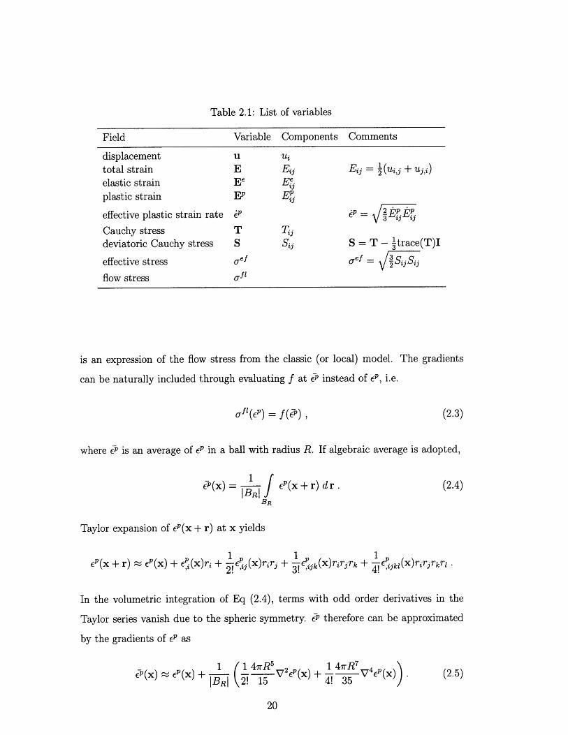
Table 2.1: List of variables
Field Variable Components Comments
displacement u Uitotal strain E Ei E = (ui, + uj,j)
elastic strain Ee Ejplastic strain EP Ej
effective plastic strain rate P P= 3 2iCauchy stress T Tijdeviatoric Cauchy stress S Sij S = T - 1trace(T)I
effective stress a e f 0 ef = SijSij
flow stress afl
is an expression of the flow stress from the classic (or local) model. The gradients
can be naturally included through evaluating f at J' instead of eP, i.e.
(2.3)
where OP is an average of eP in a ball with radius R. If algebraic average is adopted,
EP(x + r) dr .
Taylor expansion of eP(x + r) at x yields
10 (x + r) r eP(x) + j(x)ri + I Ej. (X)rirj
2! '"
1+ Pijk(X)Tirrrk3!~"
14+ Ijkl(X)rirjrkr l
In the volumetric integration of Eq (2.4), terms with odd order derivatives in the
Taylor series vanish due to the spheric symmetry. P- therefore can be approximated
by the gradients of eP as
+(x) e cP(x) +1B
IBRI1 4rRs2( +
2! 151 4rR7 V4Ep(x)
4! 35 (2.5)
(x) =BR
(2.4)
afl (Ep) = f(W) ,

Linearization of f (j) at ep leads to
f( )) f(eI) + h(eP)( P - EP) (2.6)
where h(EP) = f' (p ) is identified as hardening function. With these preparations, the
flow stress can be reformulated as follows.
fp(E ) f(EP)
f f( P ) + h(P)( i - eP)
= f (EP) + h( 1 47R5 V26 + 4 4 7 p
IBRI 2! 15 4! 35
S(EP) + h(c) ( V2EP + V 4p )
This suggests
Co = f(EP) , c1 = h(EP) 2 = h(P)
in the expression of flow stress (Eq (2.1))
Sfl(6p) = Co + C1V2Cp + C2 V4 p .
And radius R can be viewed as a problem specific internal length scale.
The foregoing interpretation has a limitation that cl and c 2 are forced to take
the same sign. The ellipticity is then only valid if h does not change sign during the
entire deformation. h > 0 represents hardening and h < 0 represents softening. In
some situation, it is desirable to include both hardening and softening behaviors in
the deformation. Based on this consideration, Aifantis argued that the interpretation
above is not necessary, and the coefficients cl and c2 can be independent of each other.
Later, Aifantis also utilized his proposed gradient model to describe the size-
dependence effects [2]. The expressions of the flow stress he presented later are more
general than Eq (2.1). Other gradient terms such as IIVCP112 also appear in the
constitutive relation in order to fit the experimental results. Among all of the strain

gradient plasticity models proposed by Aifantis, the model described by the equation
afl(eP) = o0 + he + cV 2 6p . (2.7)
is the simplest and most popular in the formulation of numerical methods.
Fleck and Hutchinson's model
The frame of variational constitutive updates to be presented in the next chap-
ter is inspired by the strain gradient plasticity model of Fleck and Hutchinson [12].
Starting from the invariants of the plastic strain gradients VEP, Fleck and Hutchinson
constructed a generalized effective plastic strain rate, and then proposed a minimum
principle for strain hardening materials. This minimum principle is an extension of
the extremum principle by Hill for the classical case of isotropic hardening materials.
Unlike Aifantis' models where the expression of flow stress is imposed a priori, the
flow rule is naturally generated from the optimal conditions of the proposed minimum
principle.
Basic assumptions in small strain isotropic plasticity are adopted, such as the
additive decomposition of elastic and plastic strains, small rotation and incompress-
ibility of plastic deformation. These assumptions can be mathematically expressed
as
E=Ee+EP, trace(E) = O .
The normality condition
= N = p s upon plastic loading
0 otherwise
from J2 flow theory is also adopted, leaving the definition of plastic loading to be
determined.
It is an important feature of the FH model that higher order stresses associated
with plastic strain gradients are explicitly introduced in the model, and the Principle

of Virtual Work is utilized to obtain the equilibrium equations. The Principle of
Virtual Work in the FH model can be expressed in the following way.
Internal virtual work:
= f T 6Ej + ESEP + miJ&E dV
= f, Tj(JEi - J6Ez) + E&P + mi<i dV
= fv Tij6Ej - SjbEEj + Ei~6 + mi56< dV
= fTijEij - SijbPNij + E&P + mi6J dV (2.8)
= fv T1jbE3j - UefEP + E P + mije& dV
= fv -Tij,jbui + (E - o ef - mi,i)&P dV + fs Tijnjbui + miniJeP dS
= External virtual work
= fs tibuz + 7B6 P dS
where E and m are the work-conjugates to the effective plastic strain and plastic strain
gradients respectively, t and 7 are the traction and higher order traction prescribed
on the boundary respectively, and n is the outer normal direction to the boundary.
Regarding the dimension, m is called the higher order stresses (or moment stresses).
The local equilibrium equations follow immediately from the variational equation
(2.8).
In the body, we have
Tij,j = 0 (2.9)
E - aef - mi,i = 0. (2.10)
While on the boundary, we get
ti = Tijnj (2.11)
7 = mini . (2.12)
In addition to the conventional equilibrium equations Eq (2.9, 2.11), Eq (2.10) and
Eq (2.12) emerge resulting from the variation with respect to eP. In the Principle of

Virtual Work (Eq (2.8)), E is the work-conjugate to the effective plastic strain, while
in the classical J2 flow theory, it is the effective stress aef that serves as the work-
conjugate to the effective plastic strain. E is therefore called the generalized effective
stress. Fleck and Hutchinson specified the plastic loading in the their gradient model
by
E=EY and E=EY (2.13)
where EY is called generalized yield stress. The gradient model of Fleck and Hutchin-
son will be complete if the evolution of EY is described.
Inspired by the minimum principle of Hill for strain hardening materials in the
classic J2 flow theory, Fleck and Hutchinson proposed the following minimum princi-
ple1 : among all the kinematically admissible fields, the exact rates of the displacement
and the effective plastic strain minimizes the following functional
I(fi, P) = jk( -- PNi) (Ekl - Nkl) + h(Ap) (p) 2 dV - tii + dS .
(2.14)
In Eq (2.14), C is the conventional fourth order elasticity tensor, the hardening
function h that comes from uniaxial tensile test is always positive and Ap is the
generalized effective plastic strain rate defined by the expression
Ap = {(ep) 2 + Aiy + BiiP + C(P)2 1} . (2.15)
The coefficients Aij, Bi and C are dependent on internal material length scales.
Expressions of these coefficients are given in Appendix A.9.
It is shown in Appendix (A.22, A.27) that the minimum {fi, iP} of I should satisfy
'Proof of this minimum principle is provided in Appendix (Theorem 1).

the following optimality conditions:
Tijnj
-&ref + h[(1 + C)iP + Bi' ] - h[A + BiP]} ,
h[Aij& + BiP]hi
= 0
= i
= -
in V
on ST
in V
on ST
(2.16)
where T is the rate of Cauchy stresses associated with {fi, 0P}.
In consistency with the conclusions derived from the Principle of Virtual Work
(Eq (2.10, 2.12)), it is natural to define
1rhi = h[AijP + 2 BiO] , (2.17)
and1
E = h[(1+f C)i+f 2Beii] . (2.18)
After applying these definitions, variational results in Eq (2.16) become identical
to the rate form of the PVW results (Eq (2.9, 2.10, 2.11, 2.12)) upon plastic loading.
Equations that govern the evolution of this elastic-plastic body are summarized below.
Equilibrium equations:
(2.19)
(2.20)
(2.21)
(2.22)
on ST X (0,Tf]
on ST x (0, T f ]
Tij,j = 0
E - eI - mi,i = 0
Tijnj = ti
mini = 7T
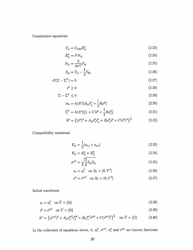
Constitutive equations:
Tij = CijklE ' (2.23)
E/ = PNij (2.24)
3Nij = 3 S (2.25)
Sj = T - 1Tkk (2.26)
e(E - EY) = 0 (2.27)
0 > 0 (2.28)
E - EY < 0 (2.29)1
rin = h(AP)[Aij& + -B ] (2.30)
1tY = h(AP)[(1+ C)ip + 1 Bj] (2.31)1
ip = {(0p) 2 + Ajji j + Bi P? + C(P) 2 } (2.32)
Compatibility equations:
1
Eij = 1 (uij + uj,i) (2.33)
Eij = E( + Ej (2.34)
,ef = (2.35)
u, = u S onSux (0,T f ] (2.36)
P = Ep,s on Su x (0, T f] (2.37)
Initial conditions:
S= on Vx {0} (2.38)
eP = Epo on Vx {0} (2.39)
AP = (ep,0)2 + A{j°~(oe ' °o + Bii p '0 + C(Ep,0) 2 2 on V x {0} (2.40)
In the collection of equations above, h, uS , ep,s, u and ep,o are known functions

and [0, Tf] is the total time interval of the evolution.
Gudmundson's model
Gudmundson generalized the Principle of Virtual Work that has been used by
Fleck and Hutchinson, where the full plastic strain tensor instead of the effective
plastic strain is considered [16]. Another important feature of Gudmundson's model
is that the classic assumption of normality of the plastic flow is abandoned.
The principle of virtual work in Gudmundson's model reads
Internal virtual work:
= f TijbEe + QijSE? + Mijk6 E?,k dV
= fy Tij (6Ei - 6 Ei) + QiJEj + MijkSEP,k dV
= fV Tj6Eij + (Qij - Sij)JEp + Mijk6 Efif,k dV
= fy -Tijjui + (Qij - Sij - Mijk,k) 6Ep dV + fs Tijnj6ui + Mijknk6SEi dS
= External virtual work
= fs ti6ui + RijJE,6 dS,(2.41)
where Q and M are the work-conjugates to the plastic strain EP and its gradient
respectively, t and R are the traction and the higher order traction prescribed at
the boundary respectively, and n is the outward normal to the boundary. The local
equilibrium equations follow directly from the variational equation (2.41).
Tij,j = 0 inV,
Qij - Sij - Mijk,k = 0 in V, (2.42)
Tijnj = ti on S ,
Mijkrk = IRj onS.
Rather than simply accepting the normality relation in classic J2 flow theory,
Gudmundson brought in the free energy and derived the normality relation based on
the plastic dissipation. Assume that the free energy density is O(Efj, Ej, E.f,k). The

plastic dissipation has the following formula
S=(Q ) E) + (Mijk
ve
= f(Q -Ve
0 )E ?i9E pj+(Mijk -a EPj,k ik dV ,
where Ve is an arbitrary volume element. This expression can be simplified as
(2.44)= Qijij + MijEkj,k dV.
V,
if definitions Qj = Qj - 7 and f~ijk = Mijk - are applied.E '3 OEij,k
As an analogue to the principle of maximum plastic work in the classic J2 the-
ory, if the plastic strain and strain gradients are prescribed, the actual stresses pair
{Qij, Mijk } will maximize the plastic work, i.e.
{Qij, Mijk} = arg max Qj Ei? + MijkEij,k (2.45)
where E is the current yield surface with the definition2
E= {{Q, Mi*jk}ij k3 iQj + L-2 ~jkMik < Y
In the definition above, L is the characteristic material length scale and EY is the
generalized yield stress.
The Lagrange function associated with the constrained optimization problem
(2.45) is
*- - 3- -* - - y£(Qy4 -kJ- + MjkE+j,k - J +L-2Mijk ijk
(2.46)
2This definition is a simplified version of the one in Gudmundson's paper. He also utilized theorthogonal decomposition of the third order tensors so that three characteristic material lengthscales are included. Nevertheless, this simplified version already contains the essential structure.
Ei,k dV
(2.43)

where A is a multiplier corresponding to the inequality constraint. Assume (Q, M) is
the maximum and A is the associated multiplier. First order necessary conditions for
the constrained optimization problem (2.45) then read
O,(Q, M, A)=O and M, (Q, M, A)=O,
which yield the following normality relations
. = 2E (2.47)
E~j,k AL-2 ijk
with definitions
A /2 P PL2EP E P= -~ i + L ij, k i j , k
In order to complete Gudmundson's model, an expression for the free energy density
V must be provided. A sample expression
(Ee, EF, Eik) CijklE EL + iL E j,k E,kZ' ' 2 U 7 Z 2 ii E iE k-iI
is offered in his paper whereIL is the shear modulus. Eij is usually not included in
the free energy density expression, so the first equation in (2.47) can be rewritten as
3 31Ej =A EQj.
Gurtin and Anand's model
Not long after Gudmundson's work, Gurtin and Anand proposed a strain gra-
dient visco-plasticity model [17]. They also abandoned the classical assumption of
normality of the flow rule regarding the non-negative requirement of plastic dissipa-
tion. When they apply the Principle of Virtual Work, the full plastic strain tensor
is used, so the equilibrium equations they obtained coincide with those in Eq (2.42).
An important feature of Gurtin and Anand's model is that the expression of the free

energy density is specified, where only the curl of the plastic strain gradient (curlE P)
rather than the full tensor (VEP) is included. They made this choice because the curl
of the plastic strain tensor is a measure of the incompatibility of the plastic strain
field and in the micro-structural configuration, it measures the local Burgers vector
[18] while other components of the plastic strain gradient tensor do not have such
physical meanings. In their formulation, they also distinguished the characteristic
material length scales in the expression of the free energy density and those in the
expression of the generalized effective plastic strain rate. The length scales in the
expression of the free energy density are identified as the energetic length scales be-
cause these length scales only appear in the back stress term in the flow rule (2.50),
which represents the energy stored in the material due to the incompatibility of the
deformation. The length scales in the expression of the generalized effective plastic
strain rate are identified as the dissipative length scales, because they only appear in
the dissipative terms in the flow rule, which presents the energy dissipated during the
plastic deformation. A sample expression of free energy density in their paper reads
1 1 2= +CijklEjEl + -IL2~EtEL EimnE n,m. (2.48)
In Gudmundson's model, the normality relations (2.47) are derived from the
first order necessary conditions associated with the constrained optimization problem
(2.45). As a result, the two equations in (2.47) have a common Lagrange multiplier.
In Gurtin and Anand's work, they did not take the principle of maximum plastic work
as a point of departure. Instead, they proposed the following normality relations that
account for the visco-plasticity effects:
do = j (2.49)MIijk =2SY( p)m" Efj,k
where
dP= j E " +12EP E~,ij,k ij,k

and S is an internal variable whose evolution is characterized by
S = H(S)dP, S(x, 0) = S
It is worth emphasizing that the non-negativeness of the plastic work in Gurtin and
Anand's model is guaranteed since the normality equations (2.49) implies that the
plastic work
dP 1. d 1QijE + MijkEi,k d= (~) EE, + 2S do)mP ,kEk > 0 .
Combination of Eq (2.49) and the second equation of (2.42) yields
1 1Sj- (-1)L2[Ei 2 Ek,jk +Ek,ik) +
3 (ijErk,rk)]
energetic backstress
p dp k.(2.50)
= S )" 13 _ 2 SY[( )m )k ,k] ,do dP do dpdissipative hardening
which is the flow rule of Gurtin and Anand's model.
Nix and Gao's model
Motivated by their analysis of indentation experiments, Nix and Gao proposed a
mechanism-based theory of strain gradient plasticity [15, 19]. The main result is that
the square of the flow stress is an affine function of the plastic strain gradient, i.e.
ao = Yo f 2 () + l (2.51)
where ao' is the initial yield stress, f is a function characterizing the uniaxial stress-
strain curve in the absence of the gradient effect, e = 2EjEj is the effective strain,
j is the effective strain gradient, and 1 is an internal material length scale.
Expression (2.51) is derived from the Taylor relation of the shear strength and the

dislocation density. The Taylor relation predicts that
7 = al-iblOT, (2.52)
where 7 is the shear strength, y is the shear modulus, b is the magnitude of the Burgers
vector, PT is the total dislocation density, and a is an empirical constant. Assume
that von Mises criterion is adopted and the total dislocation density is simply the
sum of the statistically stored dislocation density Ps and the geometrically necessary
dislocation density Pc. Eq (2.52) can therefore be reformulated as
f1' = V7 = V aybVIs +PPG . (2.53)
In the absence of gradient effects, PG vanishes and then
f1= NVa-abvp-i = 0f()
which implies
v'3aybVpb = af f(e) . (2.54)
Nix and Gao defined the effective strain gradient as
n = PGb , (2.55)
considering the dimensional requirement and some geometrical insight. Effective
strain gradient ql defined in Eq (2.55) can be viewed as the curvature of the bending
[13] and the twist per unit length in the wire torsion tests [15].
Combination of Eq (2.53, 2.54, 2.55) yields the expression of flow stress in Eq
(2.51) with the value of the internal material length scale 1 = 3a2(-) 2 b.

Chapter 3
Numerical methods for strain
gradient isotropic plasticity
3.1 Summary of current numerical methods
The initial work on the formulation of numerical methods for strain gradient
plasticity should be attributed to de Borst and Miihlhaus [5]. In their paper, they
used Aifantis' one parameter model (2.7) to provide the ellipticity of the governing
partial differential equations in the strain-softening regime. The numerical formu-
lation proposed by de Borst and Miihlhaus is a mixed method in the sense that
the displacement and the effective plastic strain are treated as nodal unknowns and
updated simultaneously. Another important feature of their approach is that weak
formulation has been applied on both the conventional equilibrium equation and the
yield condition, so that the yield condition is satisfied in the sense of distributions
rather than point-wise. de Borst and Miihlhaus did not take the Principle of Virtual
Work as a point of departure; consequently the concept of higher order stresses does
not emerge in the formulation. Only the conventional traction condition is applied
on the boundary. A potential theoretical issue with this approach is that, resulting
from the weak formulation, either the value of P or , in should be prescribed at the
elastic-plastic boundary. Regarding the continuity of the plastic strain field, they
imposed P = 0 at the internal elastic-plastic boundary. A numerical example of a

bar with imperfections at the center under uniaxial tension is used to demonstrate
that the mesh-dependence effect is eliminated during the plastic deformation with
softening.
Following the approach of de Borst and Miihlhaus, Ramaswamy and Aravas [26]
applied the mixed formulation to a two-dimensional problem, localization of plastic
flow in plane strain tension. A general expression of flow stress
Oef = O (g() + 11 gl (P)II 2 + 2 ()V2)
is adopted in the formulation they proposed, although in the numerical example, the
degenerate case with 11 = 0 and g2 - 1 is used, which is almost the same as Aifantis'
one parameter model (2.7). Engelen, Geers and Baaijens also took the approach of
mixed formulations to simulate plastic deformation in the presence of strain-softening
[8]. They introduced a so-called implicit gradient model
P - c(1),2eP = p , (3.1)
where PE is a nonlocal measure of the plastic strain. Instead of Jp , P is considered as
the primary unknown. The main advantage of this implicit model is that no additional
condition is needed on the internal elastic-plastic boundary, since Eq (3.1) is assumed
valid throughout the domain. On the external boundary, ,rni = 0 is set to ensure
that same amount of plastic deformation will be obtained no matter whether EP or PS
is chosen to measure the plastic deformation, i.e.
V dV = jvP dV.
In addition to the mixed formulations, efforts have been made to develop the meth-
ods where the displacement and the effective plastic strain are not updated simultane-
ously [21, 4, 6, 7]. In [21] and [4], the effective plastic strain Jp is defined at Gaussian
points instead of nodes. Each Gaussian point is assigned a 'super-element', which
comprises several adjacent elements in its neighborhood. p is then approximated by

a quadratic polynomial using the least square method within this super-element. The
increment of dp at each Gaussian point is directly obtained from the solution of the
linearized yield condition within the corresponding super-element, given the strain
increment. The main appeal of this approach is that the displacement is the only
nodal unknown, which makes it possible to utilize the existing finite element code
without significant modification in structure. Nevertheless, this approach means that
the solution to a globally existing second order partial differential equation including
spatial derivatives is obtained within patches (super-element). It is not clear how to
assign boundary conditions for these patches, and a more serious issue is that the
accuracy of such approximations is not guaranteed theoretically. Recently, Djoko,
Ebobisse, McBride and Reddy implemented a staggered method in the framework of
discontinuous Galerkin formulations for plane problems [6, 7]. The effective plastic
strain is discretized by discontinuous piecewise-linear elements. Aifantis's one pa-
rameter model is utilized in their formulation to demonstrate the size-dependence
effects.
3.2 Variational constitutive updates applied to Fleck
and Hutchinson's model
As already mentioned in Chapter 1, the numerical formulation based on the frame-
work of variational constitutive updates provides an alternative approach for solving
the initial boundary value problem for strain gradient plasticity theories. The key
element of building a numerical formulation that adopts this framework is to con-
struct an appropriate functional, from which the internal variables can be obtained
through minimization. Due to its minimum structure, the incremental version of the
strain gradient isotropic model proposed by Fleck and Hutchinson is taken as the
foundation of the numerical formulation in this thesis.
Assume that the displacement rate ii is tentatively prescribed, which implies that
the strain rate E is also determined. The effective plastic strain rate P can be

consistently obtained through the variation of the functional in (2.14) with respect
to the effective plastic strain, i.e.
P = arg min J(?; ii) . (3.2)
with
J(?; fl) = ijkl (Ec - N)(Ek1 - Nk) + h(Ap)(A2)2 dV - j + iiii dS .
Consistency is satisfied in the sense that if the strain rate is the exact rate, the
effective plastic strain rate obtained from the variational constitutive update will
satisfy the force balance equations and the constitutive equations in (2.16). The
stress update follows immediately from the solution to the minimization problem
(3.2)
Tij = Cijkl(JEkl - Nkl) .
Considering the definition of the generalized effective plastic strain rate (2.15)
(Ap)2 = ( p) 2 + Aij,2 + Bij iP + C(p) 2
the expression of the functional in (3.2) can be reformulated as follows.
J( P; -i) = 1 jvCiJkl(EJ - PNij)(Ek - Nkl) + h(A)(p)2 dV - -HP +iiii dS
- Mijeie - 4NjEij + CijklEjEkl dV - Fi- P + iii dS
= Mijeiej dV -j 2pNijEgij p dV - j f p dS
+ 1 Cijk kj dV - I iti dS
(3.3)
with
e = [', P, , 3, p] (3.4)

andhArt hA12 hA13 h B 1
hA21 hA 22 hA 23 hlB2M = (3.5)
hA31 hA 32 hA33 h B 3
hlB1 h B2 hIB3 h(l+C)+3 3
M is positive definite and symmetric due to the definition of Apl. Provided that N
does not degenerate to zero,
CijklNklNij = A6ij 6kl + /Iik 6 jl + Jiljk)
= [AJijNkk + P(Nj + Nj)]Nij
= 21tN jN3
= 2M-
= 3/ .
This fact has been used in in the derivation of (3.3).
The first order optimality conditions associated with the minimization problem
(3.2) read
-d i ef + h[(1 + C)Op + Bi] - {h[Aijij + Bi ]}, = 0 in V
h[Aij& + Bi]n = ?- on ST,
which coincide with the flow rule of the FH model upon plastic loading. (See Appendix
(A.27) for the derivation.)
Discretization in time
Since the plastic deformation is history dependent and irreversible, there is a need
for the algorithm to update the plastic strain. In order to update the plastic strain,
we should discretize the normality relation first. Regarding the stability issue, we
adopt backward Euler method to discretize the normality relation and the internal
'Details are offered in Appendix (Lemma 1).

variables.
Assume that [t(n), t(n+l )] is a generic interval in time. The normalized flow direc-
tion N within this increment is defined by the deviatoric Cauchy stresses at the end
of this increment, which means
N 3 S( 7 1)Ni j= - (3.6)
2 ,ef,(n+l)
The increment of the effective plastic strain is considered as an independent variable,
and we define
EP,(n+1) _ p,(n) + A p .
Discretizing the normality condition EP = PN with the flow direction defined in (3.6)
leads to
,Epnl) = E(n+ AEpNj
The generalized effective plastic strain is discretized by the following expression
Ap,(n+1 )
= Ap,(n) + AAp ,
where
AA" = ((1 + C)(ALE) 2 + A je e + BiAJAP) )
It is worth emphasizing that since the model of Fleck and Hutchinson is an
isotropic hardening model, the flow direction can be predicted by the strain increment
as follows.3 S + 1)
Nij = 2 ij - = 3dev(CijklE e) , (3.7)2 0 ef,(n+1)
where
EPTe = E )+ AEk (3.8)
is the elastic strain predictor and P is a factor that normalizes N.
With the preparation above, the functional for the variational constitutive update

is discretized as
Jh(A"?; Nj, AEjj) = j Cijkl(AEi - AcPN.j)(AEkl - AEPNkl) dV
(3.9)+ v h(Ap,(n+l))(AAP)2 dV - ArTAc dS
with AT = r (n + l ) - (n ) . The term fs, iiti is not included since it is constant for the
updates of the plastic strain.
Assuming that the strain increment AE is prescribed, the increment of the ef-
fective plastic strain AeP can be consistently obtained through the variation of the
functional (3.9), i.e.
Ade = arg min Jh(J&P; N, AEj) . (3.10)
Being analogous with the continuous case, the first order optimality conditions of
the minimization problem (3.9) yield
-Aaef + AE Y - (Ami),i = 0 in V(3.11)
Amini = 0 on S ,
given the following definitions
AE Y (h',A,(+1)AAP + hIA,,(+))((l + C)AEp + 2BiAe)
Ami = ( h'IAp,(n+l)AAP + h Ap,(n+±))(AijA&' + 1BiAeP) (3.12)
Aaef = Cijkl(AEij - AEPNij)Nkl .
These results are consistent with the results of the foregoing rate form in the sense
that convergence to the corresponding rate formula can be achieved as the time-step
approaches zero, provided that h' is finite. If the hardening function h is measured
at AAp ( ) rather than AP'( +l ) in the functional Jh, the first two definitions in (3.12)
becomeAE Y = hiA,,()((1 + C)Ae + !BijAe)
m = hA (A + (3.13)Ami = h|,A,(n)(AjjAej + BIBiAE).

3.3 Finite element formulation
Assume that a solid body occupies a domain V C R'. The boundary of this body,
S comprises two disjoint subsets ST and Su, such that S = ST U Su, q = ST n Su.
ST is the portion of the boundary where the traction t and the high order traction T
are specified, while Su is the portion of the boundary where the displacement u and
the effective plastic strain EP are specified. The initial boundary value problem can
be stated as: Find u(x, t) and cP(x, t) satisfying the initial conditions, equilibrium
equations, compatibility equations and the constitutive equations (2.19-2.40).
Assume that the deformation history of this solid body has been divided into a
sequence of increments, [t(n ), t(n+l)] C [0, Tf] is a generic increment in the deforma-
tion history and all the variables are known up to t(n ) . The incremental boundary
value problem during this generic time interval can be stated as: Find u(n+l)(x, t)
and p,(n+1l) (x, t) satisfying the equilibrium equations, compatibility equations and the
constitutive equations below:
Equilibrium equations:
Tij,j = 0 (3.14)
E - a ef - mi,i = 0 (3.15)
Tijnj = ti on ST (3.16)
mini= 7 on ST (3.17)
Constitutive equations:
T 3 = CijklEj (3.18)
AEP. = AENi (3.19)
3Ni- 2a= Si (3.20)
1Sj = T 3 Tkk (3.21)
3

AfP(E - E Y ) = 0 (3.22)
AE" > 0 (3.23)
E - EY < 0 (3.24)
Ami = h(AP)[AijAcE + 2Bi AP] (3.25)
1AE " = h(AP)[(1 + C)Acp + 1 Bj ] (3.26)
AAP= {(AP) 2 + AjA cA + BiA ZAep + C(AEP) 2 1} (3.27)
Compatibility equations:
1
Eij = 21(u±, + uj,i) (3.28)
Etj = E7 + Ez (3.29)
0eef = - Sj Sj (3.30)
Ui = uS on Su (3.31)
eP = ep s on SU (3.32)
Values at t (n) are taken as the initial conditions. Unless being specified, superscript
(n+1) is omitted in the equations above. These equations are the discrete version of
Eq (2.19-2.40) in Chapter 2, following directly from the discretization scheme in the
previous section.
3.3.1 Computational framework
Since the deformation history of the solid body is divided into a sequence of
increments, the key to building a numerical formulation is to construct an algorithm
for solving the incremental boundary value problem within a generic time interval.
Our algorithm for a generic increment from t (n) to t(n+l) is described below:
1. Update the tractions and compute the external forces Fext. Initialize the dis-
placements and the displacements increment, i.e. u := u (' ) , Au := 0.

2. Update the displacements, u := u + Au. Calculate the strain E and the flow
direction N.
3. Obtain the effective plastic strain eP and the stresses T through the variational
constitutive update.
4. Calculate the internal force Fint.
5. Check the force balance. Is IIFe"t - Fintll acceptable or not?
* yes, (.)(n+l):= (.), exit iteration.
* no, continue.
6. Calculate the consistent tangent matrix K, which is the Jacobian of the system.
7. Obtain the displacement increment Au by solving
KAu = Fext - Fint
Go to step 2.
The definitions and the expressions of terms Fext, N, Fint and K will be provided
in the next section.
3.3.2 Derivation of main equations
In this section, all the expressions of the terms that appear in our algorithm will
be derived.
Assume oa is the shape function of the displacement field at node a and Oa is the
shape function for the effective plastic strain field at node a. Then cp = E Pa and
u = uapa with nodal unknowns EP and uia.

Flow direction:
1Nj = P (CjklE~e -
6ijCmmklE e)
where
v2 =,E' = + AEkl
Internal force:
aF j To'aj dxFf= Tijpa,j dx
External force:
Assume there is no body force.
Fet =i tiP dSS T
tiS a dS- e Jd9enST
Variational constitutive updates:
The functional for the variational constitutive update is written in finite element
formulation as follows.
1J(AE; u) = 2I Cijkl[AEij - AE'PaNij][AEkl - a4E'bNkl] dx
V
h(AP)(AAP) 2 dx - ATrALpV dSV

where
(AAP) 2 = (1 + C)(AE'/a)2 + AijAEPaa,iACEbb,j + BiAEP a,i A/b
and AP has two choices, Ap (n") or AP,(n+ l ) . We adopt Ap,(n ) because it will lead to a
relatively simple formulation. The numerical examples in the next chapter show that
the convergence is not affected by this choice.
We define g(AEP; u) as the derivative of Jh(/EP; u) w.r.t. AEP.
0Jh9g =0a
= Cijkl [AEkI - .Ad/bNkl [-OaNij] dxV
+ h[(1 + C)2A "b'a + 2AjAeObb,jPa,i
V
+ Bi a,iAE b + Bi&AAPb,ia] dx - f A'ra dS
S
= J-2p/EktNklOa + 3IAbab dx
V
+1 h[(1 + C)2AIE4/bV a + 2AijA/Cb,j/a,i
V
+ Bia,iAdOb + Bi~dEb,ia] dx - ATOa dS
S
We define H(AEp; u) as the Hessian matrix of Jh(AeP; u) w.r.t. Acp .
8gaHab =
= J CijklNklNij'a)b dx
Vf Bi (3.33)+1 h(1 + C)/ab + hAij a,ib,j + h-2(a,ib + Ob,i a) dx
V
= [3/ + h(1 + C)]Oab + hAija,iVb,j + hB(a,ib + b,ia) dx .
V

The increment of the effective plastic strain A&p can be obtained by solving a
system of the linear equations
HabEP = fa
with H defined in (3.33) and
fa = 2 AEklNklia dx + Ara dS.V S
Consistent tangent matrix:
The consistent tangent matrix is the Jacobian of the system.
tent tangent matrix to solve the residual equations is essential for
convergence rate. In our specific algorithm, the consistent tangent
byOFint
K=Bu
Using the consis-
achieving a good
matrix is defined
The components of K have the expression:
Kiajb = =-- (J Tim(pa,m dx)aujb Ujb V
-J Tim ra,mdx
= ujb ,m d x .
V
Since the Cauchy stresses
Tim = Cimst(Et - (E ( + ) )
= Cim't(Est -_ (E.i)+ A EN't)),
the derivative of the Cauchy stresses with respect to the nodal value of the displace-
ments has the following expression
OTim C Es= Cimst [
9 Ujb Uj b
=(I)
OACP N t- Aep W .ojb dUjb
=(II) =(III)
(3.34)

Terms (I) and (III) in (3.34) can be determined locally:
aEst(I)- jb
OU'jb
1 10- (us,t + Ut, 8 )
2 ujb18
= (Usaa, t + Uta(Pa,s)2 cUjb1
= 2J (sob,t + 6 tPb,s) -2
(III) = t
Oujb Sujb 8t
= uSpe +Ujb 9t
(3.36)aP/ (Spre)
aUjb
Recalling the definitions of SPtr and the elastic strain predictor Ere,Epre 1 EPre
Spre = CatklEe - 6stCmmklE Je
Ee = E1( ) + AEk ,
a 1= (CstklEkpe - JstCzzklEke)Ujb 3
1 0aEPe= -(Cs - czzklst k
3 ujb
= (Cstkl - 1 zzkl1st) ( a N + AEkl)3 BUjb
= (Cstkl - Czzkl6st) (E )3 aujb1 0
= (Cstkl - -Czzklst) (Ekl)3 a ljb1 1
= (Cstkl - Czzkl 6st) (jkb,1 + OPb,k)3 2"
Identity 2 = j(SkreSkple)l implies
2/3 =OUjb
(Ee,(n) and E (n) are constants)
(3.35)
S(S.pre)aujb
3 8-3(Spre spre)-22Spre ab (SPre)
2 aOUjb

and consequently we can see
= _ (SreSkpre)-2 Spre (Spreaujb 2P aUjb
where now (S t ) has already been derived.
The term
(II)= Ocujb Ulljb
can not be determined locally, because obtaining Ap from the variational constitu-
tive update is equivalent to solving a partial differential equation including spatial
derivatives throughout the domain.
The variational constitutive update together with the predictor step implies
g(EP(u); u) = 0,
for any tentative displacements u. Since g as a function of u is constant, we have
aga 19ga A aga0= +
aUjb AEC 0 9Ujb O'Ujb
= Hac +Oujb &'U3b
with-2g, N a Ek dx
8'ujb aV ljb
= - NklPa(6 kj b,l + 6 1jCPb,k) dx.
Consequently,= - [H- g]ca
&Ujb 8aUjb
Finally, the expression of the consistent tangent matrix is obtained from the com-

bination of the equations above:
Kiajb = Cimjtoa,m b,t dx
V
2[AEP(Cmjt 0a,m ',' - 3 (Pa,i b,j) dx
V (3.37)
- J 'pIAceNimPa,mNjl(Pb,l dx
V
- 2i 2[H- 1]8a f Nim a,mO6 dx J NjlOb,1Oa dx.
V V
The symmetry of K follows immediately from the expression (3.37), which is one
advantage of the framework of variational constitutive updates as we can expect.
All the terms that appear in the computational framework have been clearly de-
fined. In the next chapter, this numerical formulation will be tested through two
benchmark examples.

Chapter 4
Numerical examples
Two examples in Fleck and Hutchinson's paper [12] are selected to examine the
numerical formulation presented in Chapter 3. One of them is the shearing of a layer
sandwiched by two rigid substrates; the other is wire torsion. Both examples are
formulated as one-dimensional problems.
The hardening function h that appears in the expression of functional (3.9) results
from a uniaxial tensile stress-strain curve, which is described by the Ramberg-Osgood
relationS= - + - (4.1)
eo Lo
where o = EEO and E is Young's modulus. With the assumption of e = Ee + EP, Eq
(4.1) can be reformulated as1
which yieldshA E ~ P
h(AP) = |P =E 1 (4.2)acp n Eo

Rigid substrate
U(t)
x2
Elastic-plastic layer xl
-U(t) -
Rigid substrate
Figure 4-1: Sandwich layer: illustration

4.1 Shearing of a layer sandwiched by two rigid
substrates
As illustrated in Fig (4-1), an infinite elastic-plastic layer sandwiched by two rigid
substrates undergoes shearing displacements on its top and bottom surfaces.
Due to the geometry of this problem, the only primary unknowns are the displace-
ment component ul(X2, t) and the plastic strain component 'P(x 2, t) = 2E2(x2, t).
Because the substrates are rigid, the dislocations inside of the layer can not exit; they
will be blocked and thus pile up when they approach the boundaries. Within the
continuum theory, this situation can be modeled as the plastic strain vanishes on the
boundaries. Associated with these considerations, the boundary conditions for this
problem are set as follows:
ul (L, t) = U(t), yP(L,t) = 0
ul(-L,t) = -U(t), 7P(-L,t) = O .
The effective plastic strain rate for this specific problem is
1 1 2(Aip) 2 = 1({ p)2+ 12(wp)2 (4.3)
3 3
with p' = _, which can be directly calculated from the definition (2.15). For
this specific problem, the functional for the variational constitutive update (2.14) is
reduced to L
J(iti, I) = 1 fl( - ,p)2 + h(AP)(A p) 2 dx 2
-L
where = 9 ' and KiP is defined in (4.3).
In the calculations, we have used the material parameters in Table (4.1), which
match those used by Fleck an Hutchinson in their paper. The calculations are per-
formed in one hundred increments in order to achieve a finial displacement of 10 0oL
at the boundaries. For each increment [t(k),t(k+)], the displacement U(t) at the

Table 4.1: Material parameters -1
Young's modulus E = 1.0 N/m 2
Poisson ratio v = 0.3Ramberg-Osgood relation n = 5 and co = 0.01Half width of the layer L = 1 mLength scales tested 1/L E [0, 0.05, 0.25, 0.5, 1]
boundary is updated in the following way
U(k +l) = U(k) + 0.1 eoL,
where L is the half width of the layer, co is the parameter in the Ramberg-Osgood
relation and U(O) = 0. Both the displacement and the plastic shear strain are dis-
cretized by linear elements. Because the convergence analysis below shows that one
hundred elements are sufficient to give converged results, we use one hundred elements
to discretize the width of the layer when obtaining the data for Fig (4-2-4-5).
Fig (4-2-4-5) exhibit the final distributions of the displacement, the plastic shear
strain, the shear stress and the generalized effective plastic strain fields from the
simulations with different internal material length scales. In these figures, only the
half width of the layer (0 < x2 _ L) is shown to emphasize the length scale effect.
From these figures, we can see that the displacement is linear only in the classical
model. The stress in all cases remains uniform through the thickness, but its value
increases significantly as the internal material length scale 1 increases. When 1 is small,
there are distinct boundary layers in the distributions of the plastic shear strain. As 1
increases, the boundary layers become thick. Associated with the distributions of the
plastic shear strain, the shape of the distribution of the generalized effective plastic
strain is concave when I is small, and it becomes convex gradually as 1 increases. The
boundary layers in the distributions of the plastic shear strain should be attributed
to the boundary condition -yP(L, t) = 0. For comparison, results from the classical
model (without essential boundary conditions for the plastic shear strain) are plotted

Displacement distribution
-2 1 1 10 0.1 0.2 0.3 0.4 0.5 0.6 0.7 0.8 0.9 1
x 2 /L
Figure 4-2: Sandwich layer: distribution of the displacement
53

Plastic strain distribution
0.5x 2 /L
0.7 0.8 0.9
Figure 4-3: Sandwich layer: distribution of the plastic strain
54

Stress distribution
I/L = 0.00
- - - 1L = 0.05
. L = 0.25
....... 1/L = 0.50
1/L = 1.00
classical model
0.1 0.2 0.3 0.4 0.5 0.6 0.7 0.8 0.9 1
x 2 /L
Figure 4-4: Sandwich layer: distribution of the shear stress
4.5
4
3.5

20
15 -
Distribution of the generalized effective plastic strainI I I I I I I I I
-- l/L = 0.00
- - - I/L = 0.05
-- 1/L = 0.25
....... 1/L = 0.50
1/L = 1.00
classical model
--
- - -
I I I I I I I I I
0 0.1 0.2 0.3 0.4 0.5 0.6 0.7 0.8 0.9 1
x2/L
Figure 4-5: Sandwich layer: distribution of the generalized effective plastic strain

in these figures. As we can expect, the plastic shear strain in the classical model is
uniform through the thickness. It is worth emphasizing that the flow rule of Fleck
and Hutchinson's gradient model will degenerate to the classical J2 flow theory as the
internal material length scale approaches zero. The numerical formulation presented
in this thesis provides the flexibility to impose boundary conditions on the effective
plastic strain even when the internal material length scale is zero, while the effective
plastic strain is not an independent variable in the classical model and no conditions
should be imposed on it. Therefore we should impose the natural boundary conditions
for the effective plastic strain in order to get the same result as the classical model
predicts. In fact, recalling the flow rule for higher order stress (2.17)
1ri = h[Avjj + - Bj]
the natural boundary condition for the effective plastic strain in this specific problem
can be written as0 = = rhini
h(1l2P')
When 1 = 0, the natural boundary condition is automatically satisfied. This means
no constraint is applied on the boundary for the plastic strain, which coincides with
the situation in the classical local model.
In Fig (4-6), the evolution of the shear stress as the displacement increases is
shown for different internal material length scales. As the length scale 1 increases,
the material exhibits a stronger response. For the cases of I = 0, the stress histories
of the simulation with essential boundary conditions and the simulation with natural
boundary conditions (classical model) almost overlap. In Fig (4-7), we show a detail of
these two stress histories, and we can find that the stress obtained from the simulation
with 1 = 0 and the essential boundary conditions is greater than the stress obtained
from the simulation with the classical model. This shows that essential boundary
condition - P = 0 has an effect on strengthening even without the strain gradients,
although this effect is relatively small.

Evolution of the shear stress
2.5
O 2
1.5
0 1 2 3 4 5U/(EoL)
6 7 8 9 10
Figure 4-6: Sandwich layer: evolution of the shear stress

Evolution of the shear stress
-- 1/L = 0.00
- - - 1IL = 0.05
- - 1/L = 0.25
....... I1L = 0.50
L = 1.00
classical model
I I--
9.4 9.5 9.6 9.7 9.8 9.9U/(eoL)
Figure 4-7: Sandwich layer: effect of the boundary conditions
2.35
2.3
2.25
2.2
2.15
2.1

Plastic strain distribution
" 20 elements
. 0 40 elements
iI V 80 elements
S- 100 elements
8--
0 i. .ii.. ..
0 0.1 0.2 0.3 0.4 0.5 0.6 0.7 0.8 0.9x2/L
Figure 4-8: Sandwich layer: convergence of the plastic shear strain
The issue of convergence has also been examined. Since the exact solution is
unknown, we conduct simultations with increasing number of elements until a satis-
factory result is obtained, i.e. when there is no more visible change. The numerical
results obtained from the simulations with twenty, forty, eighty and one hundred ele-
ments are used to test the convergence. In Fig (4-8) and Fig (4-9), the distributions of
the plastic shear strain and the displacement are plotted respectively. Convergence is
evident based on these two figures, and consequently the robustness of the numerical
formulation is demonstrated. The data in these two figures correspond to internal
material length scale 1 = 0.25L.
4.2 Wire torsion
Consider a cylindrical wire of radius R with the cylindrical coordinate system
(r, 9, z). Assume that the wire is twisted monotonically. Then the total shear strain

Displacement distribution0.12
0 .1 ................................
4 20 elements0.06 ................
0 40 elements
V 80 elements0.04 .
0.042 100 elements
-0.020 0.1 0.2 0.3 0.4 0.5 0.6 0.7 0.8 0.9 1
x2/L
Figure 4-9: Sandwich layer: convergence of the displacement
(__I _I IX__L J~__Y_ _I_ IUI-~^ ~ l~_l- .1-1^-~1il-_ 1___ ~--- ---- ------- ~1_- -.. I.. -..

is prescribed by
y(r) = 2EBo(r) = a ,
where a is the twist per unit length. Due to the geometry of this problem, the only
non-zero variable is the plastic shear strain yP(r) = 2EP.,
Assume that there is no constraint for the plastic flow at the outer boundary.
Then, associated with this situation, the boundary condition at r = R is set as
7(R, t) = 0 .
Also regarding the symmetry of this problem, the strain at the center of this cylin-
drical wire should vanish. Corresponding to this situation, the boundary condition
at r = 0 reads
-y(0, t) = 0.
Written in cylindrical coordinates, the rate of plastic shear strain tensor has the
expression1
= -(r)(eoo + ze) ,2
which results in the following nonzero gradients
p 1 1P EZ,,o -2 r-
E9z,'= Eo,r = , E' =Ezra r 2 r,- 2
Directly calculated from the definition (2.15), the generalized effective plastic
strain rate for this specific problem has the expression
( 2 1p 2 + 11(Ap' - r-1p)2 + (p)2 -+ r P'P r -2(p)2
which can be reformulated as
(A)2 = d1 -~ d2+ p +d3p

Table 4.2: Material parameters -2
Young's modulus E = 1.0 N/m 2
Poisson ratio v = 0.3Ramberg-Osgood relation n = 5 and co = 0.01Radius of the layer R = 1 mLength scales tested (-, -) e {(0, 0), (.02, .2), (2, .2), (.05, .5), (5, .5), (.2, .1)}
with
d = 11+ 1412 -2
d2 1 2*-1
da = 1l + 1In this problem, the functional for the variational constitutive update (2.14) is
reduced toR
J( P) = [a(&r - p)2 + h(AP)(ip) 2 ]27rr dr .
Since the strain field is imposed externally, solving this problem purely examines
the performance of the variational constitutive update. In the calculations, we have
used the material parameters listed in Table (4.2), which match those used by Fleck
and Hutchinson. The calculation is performed by five hundred increments in order to
achieve the final strain of 10Eo. Within each increment [t(k), t(k+l)], the twist per unit
length is updated in the following way
a(k+ l ) = a (k) + 0.1 co/R,
where co is a parameter in the Ramberg-Osgood relation, R is the radius of the wire
and a(O) = 0. The plastic shear strain is discretized in linear elements. One hundred
elements are used to discretize the radius of the wire except for the calculation for
demonstrating the convergence.
Final distributions of the plastic shear strain are collected in Fig (4-10). It is clear
that the internal length scales affect the slope of the plastic shear strain at r = R.

This fact can be explained using the flow rule for higher order stress (2.17)
1ri = h[Aij3 + - Bi ] .
Combined with the natural boundary condition
rhini = + = 0
at r = R, the flow rule for this specific problem reads
10= d3 P + 1d2 p
= 61+ 12 P + 1 (-1 + l2)r-' P .
If 11 = 212 5 0, yP' = 0 will be enforced. If 11 dominates,
P' _- r-l p = 0
will be approximately enforced, and the slope jP' s r- p > 0, since yP > 0 at r = R.
If 12 dominates,
P'+ -r- "P = 02
will be approximately enforced, and the slope jP' -lr- 1 'P < 0, since P > 0 at
r = R. The results shown in Fig (4-10) are consistent with this limiting behavior.
The evolution of the torque is collected in Fig (4-11). In this figure, we can see that
as 12 increases, the material exhibits a stronger response. In addition, we can find
that 11 has only a slight influence on the torque-twist relation. In Fig (4-11), torque
T is calculated through the following formula
T = R r rTzor drdO0 0
= j To27rr2 dr
with shear stress Tzo = A(ar - 7P) .

11 = 12 = 0
- - -11/12 = 0.1,1 2 /R= 0.2- - - 11/12 = 10,12 /R= 0.2-- - 11/12 = O.l,12 /R= 0.5
__ .. 11/12 = 0, l/R = 0.5
-"
--
-. -S
0.1 0.2 0.3 0.4 0.5r/R
0.6 0.7 0.8 0.9
Figure 4-10: Wire torsion: distribution of the plastic shear strain
30
25
20
15
I I
-
v

11 = 12 = 0- - -11/12 = 0.1,1 2 /R= 0.2- - - 11/12 = 10,12 /R = 0.2
- - 11/12 = 0.1,12/R= 0.5-. -11/12 = 10,12/R= 0.5
t % t
- -- .-
I.'V10
I-C
Urn------
I'
5 10 15 20 25aR/eo
35 40 45 50
Figure 4-11: Wire torsion: torque v.s. twist
I,

45 20 elements40 elements
o 40 elements40 V 80 elements
- 100 elements
35
30
a 25
20-
15
10
5-
0 0.1 0.2 0.3 0.4 0.5 0.6 0.7 0.8 0.9 1r/R
Figure 4-12: Wire torsion: distribution of the plastic shear strain

39-
38
37
36
35
340.75 0.8 0.85 0.9 0.95
r/R
Figure 4-13: Wire torsion: zoom-in of Fig (4-12)

The issue of convergence has also been examined. Since the exact solution is un-
known, we conduct simulations with increasing number of elements until a satisfactory
result is obtained, i.e. when there is no visible change. The numerical results from the
simulations with twenty, forty, eighty and one hundred elements are used to examine
the convergence. In Fig (4-12) and Fig (4-13), the distributions of the plastic shear
strain are plotted. Convergence is evident based on these two figures; consequently
the robustness of the numerical formulation is demonstrated. The data in these two
figures correspond to internal material length scales 11 = 0.2R and 12 = 0.1R .

70

Chapter 5
Discussion and conclusions
5.1 Fleck and Hutchinson's model revisited
In 2009, Evans and Hutchinson assessed the model of Nix and Gao and also the
model of Fleck and Hutchinson (FH model) using the simple bending test as an
example [9]. Two main conclusions were drawn in their paper. One conclusion is that
the expression of the generalized effective plastic strain rate in Fleck and Hutchinson's
model (2.15)
lip = {(ip) 2 + Ajii + B 9,±P + C(AP) 2 2
should be replaced by the following expression
AP = 0P + [Aj i P + Bi p + C( P)2] , (5.1)
because the resulting model will 'correlate with the well-established square root size
scaling trends found in hardness and other tests'. The other conclusion is that the
variational structure of Fleck and Hutchinson's model should be retained because
of its flexibility to impose boundary conditions associated with the effective plastic
strain.
Although the new definition of the generalized effective strain rate (5.1) extends
the ability of the FH model to match a wide range of the experimental data, it

also breaks the mathematical structure of the original FH model. Rates (fi, iP) that
minimize the functional (2.14)
I(i, iP) = 3 j CijkI (ij - Nij)(E kl - Nkl) + h(A)() 2 dV - Tiii + 4 dS .
may not be smooth. The first numerical example in the previous chapter, shearing of
a layer sandwiched by two substrates, is a good example to explain this smoothness
issue. In the original FH model, the generalized effective plastic strain rate is
(Ap) = ( p)2 + _ p 2( ')223 3
In the improved model, it reads
1 1
The higher order stress corresponding to this generalized effective plastic strain rate
is
ml= h l'P + l1 ') . (5.2)
(See Appendix (A.27) for the derivation.) Due to the symmetry of this problem, the
plastic shear strain rate should be an even function, which means
/P(x2, t) = "P(--x2, t), for 0 < x2 < L.
If the plastic strain gradient /P' exists and is continuous,
P'(x2,t) = - P'(-x 2 , t), for 0 < x 2 < L ;
consequently at the center of the layer
y'(0, t) = 0.

Again due to the symmetry of this problem, the plastic shear strain rate is always
positive at the center of the layer, which implies that
is ill-posed at the center of the layer. As a result, the higher order stress defined in
(5.2) is ill-posed too, and the equilibrium equation (A.27) that involves the divergence
of the higher order stresses
tY - cre _ rhi,i = 0
is not well defined. All these issues suggest that the assumption of the continuity of
P' must be abandoned in the improved model.
In 2009, Fleck and Willis proposed a strain gradient plasticity model that can also
be considered as an improvement of the original Fleck and Hutchinson's model [14]. In
their work, the definition of the generalized effective plastic strain (2.15) is retained,
but the generalized effective stress is redefined in order to satisfy the thermodynamics
requirement. In the original FH model, the generalized effective stress E is exactly
the work-conjugate to p , while in the model of Fleck and Willis, it comprises both
the work-conjugate to eP and the work-conjugate to e',. Assume that the generalized
effective plastic strain rate is defined by the expression
Ap = {(p) 2 + Aij,)'j + B-i p? + C(p) 2 2
Corresponding to this definition, the generalized effective stress in Fleck and Willis'
model is defined by
- ([A-1]ijrirj) 2
with
All A 12 A 13 !B 1
A21 A22 A 23 !B 2A =A31 A32 A33 2B3
B 1 !B 2 !B 3 1+C

and
r = [mi, m 2, m3, Q, 1
where m is the higher order stresses and Q is the work-conjugate to the effective plastic
strain EP. Associated with the new definition of the generalized effective stress, Fleck
and Willis presented the following normality relations
,, A -([-]ijj) (5.3)
and
= A = - ([A-1]4yrj) . (5.4)
With these normality relations, the non-negativeness of the plastic work is guaranteed,
since the plastic work
S+ M 1 = AP([Ai-1]ijrirj) = Z& > 0.
Another feature of Fleck and Willis' model is that the effect of interface is consid-
ered. They believed that both the jump in the plastic strain and the increment in the
mean plastic strain at the interfaces induce dissipation and consequently strengthen
the response of the material.
5.2 Other problems with coupled fields
The initial boundary value problem from strain gradient isotropic plasticity theo-
ries is one specific example of the problems with coupled fields. In the strain gradient
isotropic plasticity theories, the displacement and the effective plastic strain fields are
coupled. There are also some other problems involving the coupled fields, such as the
thermal elastic models, the thermal plastic models and the gradient damage models.

5.2.1 Gradient damage model
The initial boundary value problem from the strain gradient damage theory is
another example of the problems with coupled fields [31]. In particular, there are some
similarities between the governing equations of the strain gradient damage theory and
the governing equations of the strain gradient isotropic plasticity theories presented
in this thesis.
The displacement field u and a scale field , the equivalent strain, are two coupled
fields in the strain gradient damage model presented in [31]. The governing equations
of this damage model are listed below.
Equilibrium equation:
Tij,j + fi = 0 ,
where T is the Cauchy stress tensor and f is the body force.
Constitutive equations:
Ti = (1 - D(i)) CijklEkl (5.5)
k(- K) = 0 (5.6)
> 0 (5.7)
-. < 0 (5.8)
-= Eeq + C2 V26eq (5.9)
0 if < n;o
D() = 1 (o )if o (5.10)
1 if > _ r c
where 6eq is an invariant of the local strain tensor, K is the maximum positive value
of the equivalent strain in the history, c is an internal material length scale and D(r')
describes the influence of the maximum equivalent strain K on the elastic response.
When n is less than o, the response of the material is fully elastic. As n increases, the
damage develops and the elastic response is weakened by a factor of D(r). Finally,
when n reaches C, the elastic response is no longer valid, and the material is totally

damaged.
The strain gradient damage model above is an elasticity model, and in principle
5 can be expressed explicitly in term of the displacement u once the expression of
the Ceq is provided. Nonetheless, with the structure rather than the dimension in
consideration, we can find that Eeq , 5 and r correspond to p , E and EY respectively.
5.3 Conclusions
A numerical formulation based on the framework of the variational constitutive
update has been presented to solve the initial boundary value problem from the
strain gradient isotropic plasticity theories. Various strain gradient isotropic plasticity
models have been summarized and compared in Chapter 2. Among these models,
Fleck and Hutchinson's model is adopted by this numerical formulation because it has
a relatively simple form and is sufficiently general. The numerical formulation based
on the variational constitutive update is constructed and compared to the current
numerical methods in Chapter 3. The robustness of this numerical formulation is
verified through the finite element implementation on the benchmark examples in
Chapter 4.
As discussed at the beginning of this chapter, the model of Fleck and Hutchinson
has been improved by the two authors separately. It can be a possible extension of
current work to apply the numerical formulation for these improved models. Imple-
menting this numerical formulation to other coupled fields problems, such as the gra-
dient damage model, is another possible extension. There is also some other possible
future work, such as applying the current numerical formulation for three-dimensional
problems, testing the combinations of the finite element spaces of the displacement
and the effective plastic strain fields, and extending the current numerical formulation
for the large deformation and dynamic problems.
The long-term objective of this work is to construct a robust and efficient compu-
tational framework for the strain gradient crystal plasticity theories, especially for the
investigation on the tissue level problems. The experiences and knowledges gained

from constructing the numerical formulation for the strain gradient isotropic plastic-
ity theories provide a solid foundation for the author to move towards the long-term
objective.

78

Appendix A
A.1 Expression of the generalized effective plastic
strain rate
The generalized effective plastic strain rate in the gradient model of Fleck and
Hutchinson has the expression
(i)2 (p)2 A+ij ± B ip + C(P) 2
where Aiy, Bi and C depend on three internal material length scales. In this section,
this expression will be explained.
The generalized effective plastic strain rate AP comprises the plastic strain rate
Ep and its gradients. Perhaps the most intuitive way to define AP is to adopt the
expression below:2 -
Sp(A. 1)
= (p)2 +12( Ej,kEj,k)
Eq (A.1) does include the contribution from the gradients of the plastic strain, how-
ever it only contains one parameter. In order to provide more flexibility for data
fitting, it is natural to consider other invariants in addition to Ej,kEj,k and to intro-
duce more internal material length scales. Define
Pijk = E-ij,k '

In general, there are twelve independent invariants of degree two for a third order
tensor, which can be written as follows:
PijkPijk, PijkPikj, PijkPjik, PijkPjki, PijkPkij, PijkPkji , (A.2)
and
PiijPjkk, PiijPkjk, PiijPkkj, PijiPjkk, PijiPkjk, PjiiPjkk. (A.3)
In the strain gradient plasticity model, Pijk = EP),k is not a general third order tensor.
In the model of Fleck and Hutchinson, it is assumed that the plastic deformation
is incompressible, and the strain rate Ep is symmetric. These assumptions can be
expressed mathematically as
Piik = 0, Pijk Pjik (A.4)
Because of these assumptions, the number of the invariants is reduced to three. These
invariants are
PijkPijk, PijkPikj, PjiiPjkk. (A.5)
Therefore, we can assign three parameters, and define the generalized effective plastic
strain as follows:
(Aip)2 = (p)2 + ClPijkPijk + C2PijkPikj + C3PjiiPjkk , (A.6)
where c1, c2 , c3 are three parameters with the dimension of the square of length. Ex-
pression (A.6) is already general, however it is not satisfying because the invariant
PijkPikj may take negative value, and the necessary condition for
C1PijkPijk + C2PijkPikj + C3PjiiPjkk > 0
is not clear. In order to simplify the requirement for choosing the internal material
length scales, Fleck and Hutchinson adopted an orthogonal decomposition (Details

can be found in [12])(1) (2) (3)
Pijk = Pijk + Pijk + Pijk
and defined the generalized effective plastic strain as follows:
= () 2 + L 2()(1)+ 4L (2) (2 8 (3 (3 (A.7)(1) ( ikijk + 2ijkik + 3 3Pijkyk"(
Since Pijk = Epj,k = (PNij),k = ,kNij OPNij,k , the expression (A.7) can be reformu-
lated as
(Ap) 2 _ (p) 2 + Aijj p + BiP'iP + C(?p) 2 . (A.8)
In the definition above, parameters Aij, Bi, C have the following expressions.
A,= L ( ij + " Njp) + epi,rNqr(L2epjvNq + LjeqjvNpv)
Bi = LN2 (N - gNpNpq,q)S+2eprNpq(pi,q 15 + z e N
+2epir Nr( Le,,N,,, 2+ LaeqvNpv, )
S= L (Nij,k Nij,k + 2Njk,i) - 4Nki,iNkj,j)
+epirNqr,i(L,, epNq,,, + L3equvNP ,u) ,
where L = L 2 8 , L 2 = !L2 2_ 8L 2 and eijk is the alternating symbol. Derivations2 3-2 5 33
of these expressions can be found in [12, 27].
A.2 Proof of the minimum principle
Following the treatment in [14], definitions
All A 12 A13 !B 1
A21 A22 A23 !B 2
A31 A32 A33 2B3
1B1 !B 2 IB 3 1+C2 7 2
(A.10)
and
(A.11)
(A.9)
e = [i , 2> 2P3, P]'

are introduced to simplify the derivation.
plastic strain rate AP can be rewritten as
(A=P) 2 = Aijeej.
The following lemma will be used in the proof of the minimum principle.
Lemma 1. The matrix A defined in (A.10) is symmetric and strictly positive definite
if the flow direction N does not degenerate ( NjNij = holds).
Proof. The symmetry of A is obvious based on the expression (A.10).
For any e E R 4, we can define
Pijk = ekNij + e4Nij,k . (A.12)
Because Pijk = Pjik and Piik = 0, there is a unique orthogonal decomposition ([12, 27])
(1) (2) (3)Pijk = Pij k + Pijk Pijk
As a result, we can rewrite Aijeiej as follows:
3 3
Aijeiej = (e4) 2 + AijeieJ + 1 Bieie4 + C(e 4) 2 (A.13)i,j=l i=1
=(e 4 ) 2 + +i2 M+ - 2Pi2)p2) + L (3) (3p (A.14)
which implies
Aijeiej > 0
for any e, and A is positive definite.
When Aijeiej = 0, Eq (A.14) implies e4 = 0 and k) = 0 for all i,j,k,m E
{1, 2, 3}, which yieldsPijk (1) (2) (3) =0.
ijk = pijk + pijk + pijk
Because of the definition in Eq (A.12), we have ekNij = 0 for all i, j, k E {1, 2, 3}.
With these definitions, the generalized

Using the condition NijNij = a, we can get
3o = (ek) 2jNij = (k ,
from which ek = 0 for k E {1, 2, 3} is obtained immediately. In sum, e = 0 when
Aijeiej = 0 . O
The minimum principle in the strain gradient model of Fleck and Hutchinson is
stated in the following theorem:
Theorem 1. Assume that a solid body occupies a domain V E R3 with boundary
S = ST U Su. Traction rates t and - are applied on ST. Velocity and effective plastic
strain rate {ii, P} are prescribed on Su with SSul > 0. Then the exact rates {f*, EP*}
are a unique minimum of the functional
I(f7i, e) -1 Cijklt ij - N)(fij kl, - Nkl) + h(Ap) (Ap) 2 dV -f tiii + f' dS ,
on the set W, which is defined by
= {{ii, P} E H 1 (V, 3 ) x H'(V, R)I f = &o and 0" = Fo on Su, ip 2 0, 'P(E - EY ) = 0}
Proof. Assume {l*, *} E are the exact rates. For any variable (.) and the vari-
able with star (.)*, denote the difference operater as A(*) = (.) - (*)*.
The functions
1 1Ve(W) - CijklWijWkl and VP(()= 2h2
are convex and smooth with respect to their own variables. Therefore the following

inequalities for the convex functions hold:
a VeAVe - WwAW,
8VP
AVP > - I|P .0(
(A.15)
(A.16)
The difference between the value of the functional at an arbitrary (fi, P) E 0 and
the value of the functional at {fi*, P*} can be written as follows:
I(i, e) - I(u*, p*)
Ve(Ee) - Ve(te*) + VP((Aj) - VP(A p *) dV -
ST
Ti (A, - AEj) + hAP*AAP dV -
Til (,Aj - AEj) + hAP*AAP dV -
(Ak, - AEj) + hAP*AAP dV
V-'•*AkP + hAP*AAP - ri 4AP - rih
ti Ai + ~i~P dS
itAiai + i-A? dS (T*n = ti, n*i = ), =
I °,TijnjA/i + rn* niAe dS
tj, + + + m i+ ,rie + r4* dV
A dV (T'Ti, = 0)
= ( -&ef* - (i)A + hAP*AAP - r *A dV (TdV i = &ef*o~P )
First of all, for simplicity, assume P* > 0 holds throughout the domain. Then
1* = Y = h[(1 + C)P* + B P* .2 it
CijkIE *AEj + hiP*AAP dV -
i/Aiti + ~iA p dS=V
>V
=JV-f=/V
-JV
=JV

As a result, we can obtain
*e + rl2 h.p
1= h[(1 + C)iP* + BjBi] +
2
1
h[AiP* + Bp* *]
+ p'& *) + Aj&* Pj]
(A.18)
= hAije ej ,
and also the identity
z*&'* + r.*. = hAije*e* = h(AP*)2
which is a special case of Eq (A.18). Now, continue the proof from the inequality
(A.17).
I(i, iP) - I(fi*, P*)
hAP*(AP - AP*) - - '*) - ( -- ) dV
V
h= hP*AP - Ci* - rh,;P - h(AP*)2 + E*
V
= Jh*AP - i - ,i dV
V
= h(Aieiee) (Aklekel)" - Aije ej] dV
v
+ riA* dV
(A.19)
>0
In the last inequality of Eq (A.19), Cauchy inequality has been used in the following

way:
A 3eie j = (e*)TAe-1-1
= (e*)'AAe
= (Ae*)'(Ale) (A.20)
[[]kIe*) 112 l[- ell 2
= (Aiee*)2(Aklekel) 3
where A is symmetric and strictly positive definite upon plastic loading (Lemma 1).
Up to now, the proof is achieved for the case that plastic loading occurs throughout
the domain. For a general situation, the proof follows from the decomposition of the
domain V:
V = {x E VI * > O} U {x E V * = 0}.
Starting from the inequality (A.17),
I(u, P) - I(I*, ~P*) -J*A - r F+ hAP*AAP dV
V
J -*A - AhA + hAP*AAP dV
{xEVI p*>o}
+± f - *'AtP n*L + hAp *AP dV+ * - hA, + hAp*AAP dV
{xvl p*=o)
>0.
The last inequality holds because aP* = 0 implies E* < 0 or the current generalized
effective stress E is strictly less than the current generalized yield stress Ey . When
E* < 0 , the integrand -E*P is nonnegative. When the current generalized effective
stress E is strictly less than CE, the stress state is not on the yield surface, which
implies iP = 0 and the integrand is also zero. Therefore, no matter which case occurs,

the integrand -t*eP is always nonnegative.
In sum, the exact rates {(*, **} are a global minimum. Conditions for the con-
vexity inequalities (A.15, A.16) and Cauchy inequality (A.20) to become equalities
are
Ee = e* and AP = AP*,
which suggest that for any {f, P} cE 3 satisfying AI = 0, the equalities 0 =
P~* and E = E* must hold in the domain. Since only the isotropic material is
considered here, the elasticity tensor has the expression
Cijkl = A6ij6kl + P(ik62 l + 6il6jk)
with Lame constants A > 0 and / > 0. This guarantees that the H1 norm of the
displacement and the energy norm of the strain induced by the displacement are
equivalent on HJo(V) (Page 274 in [20]). As a result, E = E* in V together with
Sul > 0 yields
i = i* a.e. in V .
Finally, the proof of the uniqueness of the minimum is complete.
A.3 Derivation of the optimality conditions
In this section, the optimality conditions associated with the functional (2.14) in
the Fleck and Hutchinson's model are derived based on a general expression of the
generalized effective plastic strain rate.
The general expression of the generalized effective plastic strain rate reads
' = {(IP) + [Ai{ + Bi + C(P)2]} for 1 < 5 2. (A.21)
Assume {Ii, P} is a stationary point of the functional (2.14) with the generalized
effective plastic strain rate defined in Eq (A.21); then the first order variation of the

functional should be zero.
The variation with respect to ii reads
I( t + t6i, iP) - I(i, i)0 = lim + t ) V i s.t. it = 0 on Sut-*O t
= Cijkl(Eij - PNiij)GEij dV - i iti dS
= (JA dV - i - i6is dSV S
f i j1ikj6Eij dV - J tiii6i dS
V S
= -i,jwit dV + T ijnj tbi dS- it uiti dS
V S S
= J-Th 6iti dV + J(inj - i)6i dS.V S
Since 6it is arbitrary, the variational equation above yields the conventional equilib-
rium equations
Tij, j=0 in V and Tjnj=tionST. (A.22)
In order to simplify the notations, a 4 by 4 matrix
All
A 21
A 31
1B1
A 1 2
A 22
A 32
iB2
A 1 3
A 2 3
A 33
2 3
1Bi
iB25 2
iB3
C
(A.23)
and a vector e = [iP, , 2 3, 3P]r are introduced to derive the variational results with
respect to P. With these definitions, the contribution of the plastic strain gradients
in the generalized effective plastic strain rates can be simplified as
AjjiP + Bi + C(0)2 = iijeiej

Define the set of the material points that undergo plastic loading by
VP = {x E VI 0 > 0o} ,
and then the set for admissible ip can be specified by
S= {5Pl 8P = O if x e V \ VP or x E S} .
The variation with respect to iP reads
0 lim I( fi, p + tep) - I(fi, P)t--+0 t
= 6(A)2 dV - J i-6 dS -VP ST
= [( P)" + (Aijeiej)u]-6[(iVP
V & E -
TklNklJ dV
12)" + (Aijeiej)y] dV - f i&P dS -
ST
-- + -( ijeiej) 2] - [,(P) fL- 1&P + Lt- ( e ) P ej) -12A^ekSe l] dV/= [(A)+ 2 klek6] dV
VP
- f i-6 P dS - J 6ef 6 P dV
ST VP
= h[(~)" + (Aj eie) A 2[(P)-l~P + (Aijeej) 2 Aklek6 el] dV
- J+# P dS - f &ef P dV
ST VP
h[(P)" + (Aijeiej)] l[)- . ( Aijeie)' -2 + C)] &' dV
'P
+ h[(e) + (Aijeiej)9] [(Ajeie.)f-'(Akl k 6+ P)l& dVVP
- 6ST dS - J VP dV
ST VP
= 1(a,, 01 - d&ef)&P dV -VP
6ST dS+ST
S/ nri P dS3VP
(A.24)
J ef P dV
VP
VP
V

Divergence theorem is applied to eliminate JSc, from the volumetric integration in the
last equation. The set aVp represents the surface of the domain VP, which can be
partitioned as follows:
aVp = (&VP n V) U (&Vp n Su) U (OV p n ST) . (A.25)
For x E (8VP n V) U (&Vp n Su), we have JP = 0. Also it is reasonable to assert that
&V P n ST = ST, since the higher order traction 7 is only associated with the plastic
loading. With these considerations, Eq (A.24) can be written as
0 = J(a - , - &ef )&P dV - J -&P dS + fJ znl6? dS
VP ST aovp (A.26)
= (a - ,, - d&ef ) dV + J (01ni - f) P dS
VP ST
Since JeP is arbitrary, the variational equation above yields the non-conventional
equilibrium equations
a - 01, - d& f = 0 in V and P1n, = + on ST. (A.27)
This is as far as the variation can take us. In the next section, we will introduce some
definitions to explain these variational results.
Comments
Regarding the results derived from the Principle of Virtual Work (Eq (2.10))
E = mi,i + " ef in V and mini = 7 on ST
and also the structure of the variational results (A.27), it is natural to define the
rate of the generalized yield stress and the rate of the higher order stresses by the

following expressions:
E = a = h[(P)" + (Aijeiej)2 ] -1[(P)p-2 + (Aijeiej)p-( k + CeP)]
rhi = p, = h[(P)" + (A ijeej)-]2 [(Aijeiej)f-l(AklPk + 2)],
(A.28)
1 = 1, 2,3.
(A.29)
With these definitions, the variational results (A.27) can be reformulated as fol-
lows:
thni = i
in V P ,
on ST .
(A.30)
(A.31)
Eq (A.30) describes the yield condition upon plastic loading, while Eq (A.31) describes
the rate form of the higher order traction boundary condition.

92

Bibliography
[1] E.C. Aifantis. On the role of gradients in the localization of deformation and
fracture. International Journal of Engineering Sciences, 30:1279-1299, 1992.
[2] E.C. Aifantis. Strain gradient interpretation of size effect. International Journal
of Fracture, 95:299-314, 1999.
[3] E.C. Aifantis and H.B. Muhlhaus. A variational principle for gradient plasticity.
International Journal of Solids and Structures, 28:845-857, 1991.
[4] R.K.A. Al-Rub and G.Z. Voyiadjis. A direct finite element implementation of
the gradient-dependent theory. International Journal for Numerical Methods in
Engineering, 63:603-629, 2005.
[5] R.D. Borst and H.B. Muhlhaus. Gradient-dependent plasticity: formulation and
algorithmic aspects. International Journal for Numerical Methods in Engineer-
ing, 35:521-539, 1992.
[6] J.K. Djoko, F. Ebobisse, A.T. McBride, and B.D. Reddy. A discontinuous
Galerkin formulation for classical and gradient plasticity - Part 1: Formula-
tion and analysis. Computer Methods in Applied Mechanics and Engineering,
196:3881-3897, 2007.
[7] J.K. Djoko, F. Ebobisse, A.T. McBride, and B.D. Reddy. A discontinuous
Galerkin formulation for classical and gradient plasticity - Part 2: Algorithms
and numerical analysis. Computer Methods in Applied Mechanics and Engineer-
ing, 2007.

[8] R.A.B. Engelen, M.G.D. Geers, and F.P.T. Baaijens. Nonlocal implicit gradient-
enhanced elasto-plasticity for the modelling of softening behaviour. International
Journal of Plasticity, 19:403-433, 2003.
[9] A.G. Evans and J.W. Hutchinson. A critical assessment of theories of strain
gradient plasticity. Acta Materialia, 57:1675-1688, 2009.
[10] E. Fancello, J.-P. Ponthot, and L. Stainier. A variational formulation of con-
stitutive models and updates in non-linear finite viscoelasticity. International
Journal for Numerical Methods in Engineering, 65:1831-1864, 2006.
[11] N.A. Fleck and J.W. Hutchinson. Strain gradient plasticity. Advances in Applied
Mechanics, 33:295-361, 1997.
[12] N.A. Fleck and J.W. Hutchinson. A reformulation of strain gradient plasticity.
Journal of the Mechanics and Physics of Solids, 49:2245-2271, 2001.
[13] N.A. Fleck, G.M. Muller, M.F. Ashby, and J.W. Hutchinson. Strain gradient
plasticity: Theory and Experiment. Acta Materialia, 42:475-487, 1994.
[14] N.A. Fleck and J.R. Willis. A mathematical basis for strain-gradient plasticity
theory-part i: Scalar plastic multiplier. Journal of the Mechanics and Physics of
Solids, 57:161-177, 2009.
[15] H. Gao, Y. Huang, W.D. Nix, and J.W. Hutchinson. Mechanism-based strain
gradient plasticity I: Theory. Journal of the Mechanics and Physics of Solids,
47:1239-1263, 1999.
[16] P. Gudmundson. A unified treatment of strain gradient plasticity. Journal of the
Mechanics and Physics of Solids, 52:1379-1406, 2004.
[17] M.E. Gurtin and L. Anand. A theory of strain-gradient plasticity for isotropic,
plastically irrotational materials. Part II: Finite deformations. International
Journal of Plasticity, 21:2297-2318, 2005.

[18] M.E. Gurtin and Paolo Cermelli. On the characterization of geometrically nec-
essary dislocations in finite plasticity. Journal of the Mechanics and Physics of
Solids, 49:1539-1568, 2001.
[19] Y. Huang, H. Gao, W.D. Nix, and J.W. Hutchinson. Mechanism-based strain
gradient plasticity II: Analysis. Journal of the Mechanics and Physics of Solids,
48:99-128, 2000.
[20] T.J.R. Hughes. The finite element moethod: Linear static and dynamic finite
element analysis. Dover Publications, Inc, NewYork, 2000.
[21] Xikui Li and S. Cescotto. Finite element method for gradient plasticity at large
strain. International Journal for Numerical Methods in Engineering, 39:619-633,
1996.
[22] L. Noels and R. Radovitzky. An explicit discontinuous Galerkin method for
non-linear solid dynamics. Formulation, parallel implementation and scalability
properties. International Journal for Numerical Methods in Engineering, 2007.
,In press.
[23] M. Ortiz and A. Pandolfi. A variational Cam-clay theory of plasticity. Computer
Methods in Applied Mechanics and Engineering, 193:2645-2666, 2004.
[24] M. Ortiz and L. Stainier. The variational formulation of viscoplastic updates.
Computer Methods in Applied Mechanics and Engineering, 171:419-444, 1999.
[25] R. Radovitzky and M. Ortiz. Error estimation and adaptive meshing in strongly
nonlinear dynamic problems. Computer Methods in Applied Mechanics and En-
gineering, 172:203-240, 1999.
[26] S. Ramaswamy and N. Aravas. Finite element implementation of gradient plas-
ticity models Part I: Gradient-dependent yield functions. Computer Methods in
Applied Mechanics and Engineering, 163:11-32, 1998.

[27] V.P. Smyshlyaev and N.A. Fleck. The role of strain gradients in the grain size
effect for polycrystals. Journal of the Mechanics and Physics of Solids, 44:465-
495, 1996.
[28] N.A. Stelmashenko, M.G. Walls, L.M. Brown, and Y.V. Milman. Microindenta-
tions on W and Mo oriented single crystals: an STM study. Acta Metallurgica
et Materialia, 41:2855-2865, 1993.
[29] J.S. Stolken and A.G. Evans. A microbend test method for measuring the plas-
ticity length scale. Acta Materialia, 46:5109-5115, 1998.
[30] K. Weinberg, A. Mota, and M. Ortiz. A variational constitutive model for porous
metal plasticity. Computational Mechanics, 37:142-152, 2006.
[31] G.N. Wells, K. Garikipati, and L. Molari. A discontinuous Galerkin method
for strain gradient-dependent damage. Computer Methods in Applied Mechanics
and Engineering, 193:3633-3645, 2004.
[32] Y. Xiang and J.J. Vlassak. Bauschinger and size effects in thin-film plasticity.
Acta Materialia, 54:5449-5460, 2006.
[33] H.M. Zbib and T.D. de la Rubia. A multiscale model of plasticity. International
Journal of Plasticity, 18:1133-1163, 2002.


![Variational problems with non-constant gradient constraints€¦ · Evans studied general linear elliptic equations with a non-constant gradient constraint in [5] and his regularity](https://img.dokumen.tips/doc/110x75/5fbcbebac166f215ac7259bd/variational-problems-with-non-constant-gradient-constraints-evans-studied-general.jpg)