Eurographics Symposium on Rendering 2017P. Sander and M. Zwicker(Guest Editors)

Volume 36 (2017), Number 4

Variance and Convergence Analysis ofMonte Carlo Line and Segment Sampling

Gurprit Singh Bailey Miller Wojciech Jarosz

Dartmouth College

AbstractRecently researchers have started employing Monte Carlo-like line sample estimators in rendering, demonstrating dramaticreductions in variance (visible noise) for effects such as soft shadows, defocus blur, and participating media. Unfortunately,there is currently no formal theoretical framework to predict and analyze Monte Carlo variance using line and segment sampleswhich have inherently anisotropic Fourier power spectra. In this work, we propose a theoretical formulation for lines andfinite-length segment samples in the frequency domain that allows analyzing their anisotropic power spectra using previousisotropic variance and convergence tools. Our analysis shows that judiciously oriented line samples not only reduce thedimensionality but also pre-filter C0 discontinuities, resulting in further improvement in variance and convergence rates. Ourtheoretical insights also explain how finite-length segment samples impact variance and convergence rates only by pre-filteringdiscontinuities. We further extend our analysis to consider (uncorrelated) multi-directional line (segment) sampling, showingthat such schemes can increase variance compared to unidirectional sampling. We validate our theoretical results witha set of experiments including direct lighting, ambient occlusion, and volumetric caustics using points, lines, and segment samples.

CCS Concepts•Computing methodologies → Ray tracing; •Mathematics of computing → Stochastic processes; Computation of trans-forms;

1. Introduction

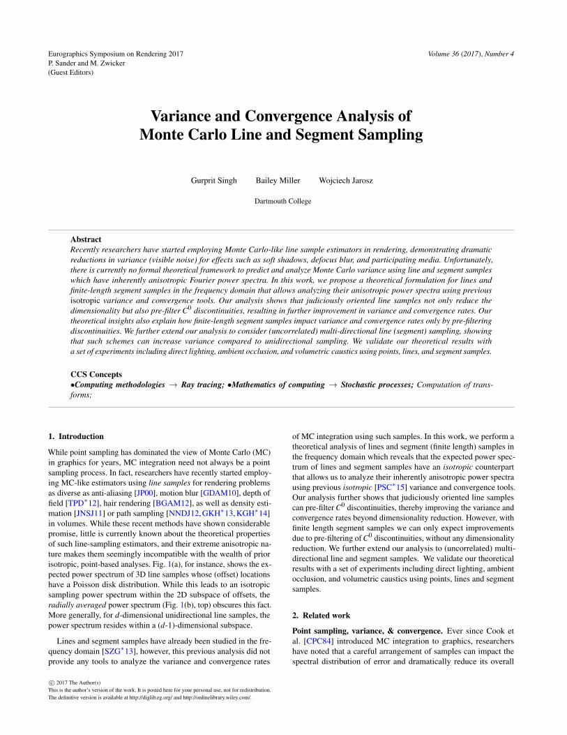
While point sampling has dominated the view of Monte Carlo (MC)in graphics for years, MC integration need not always be a pointsampling process. In fact, researchers have recently started employ-ing MC-like estimators using line samples for rendering problemsas diverse as anti-aliasing [JP00], motion blur [GDAM10], depth offield [TPD∗12], hair rendering [BGAM12], as well as density esti-mation [JNSJ11] or path sampling [NNDJ12, GKH∗13, KGH∗14]in volumes. While these recent methods have shown considerablepromise, little is currently known about the theoretical propertiesof such line-sampling estimators, and their extreme anisotropic na-ture makes them seemingly incompatible with the wealth of priorisotropic, point-based analyses. Fig. 1(a), for instance, shows the ex-pected power spectrum of 3D line samples whose (offset) locationshave a Poisson disk distribution. While this leads to an isotropicsampling power spectrum within the 2D subspace of offsets, theradially averaged power spectrum (Fig. 1(b), top) obscures this fact.More generally, for d-dimensional unidirectional line samples, thepower spectrum resides within a (d-1)-dimensional subspace.

Lines and segment samples have already been studied in the fre-quency domain [SZG∗13], however, this previous analysis did notprovide any tools to analyze the variance and convergence rates

of MC integration using such samples. In this work, we perform atheoretical analysis of lines and segment (finite length) samples inthe frequency domain which reveals that the expected power spec-trum of lines and segment samples have an isotropic counterpartthat allows us to analyze their inherently anisotropic power spectrausing previous isotropic [PSC∗15] variance and convergence tools.Our analysis further shows that judiciously oriented line samplescan pre-filter C0 discontinuities, thereby improving the variance andconvergence rates beyond dimensionality reduction. However, withfinite length segment samples we can only expect improvementsdue to pre-filtering of C0 discontinuities, without any dimensionalityreduction. We further extend our analysis to (uncorrelated) multi-directional line and segment samples. We validate our theoreticalresults with a set of experiments including direct lighting, ambientocclusion, and volumetric caustics using points, lines and segmentsamples.

2. Related work

Point sampling, variance, & convergence. Ever since Cook etal. [CPC84] introduced MC integration to graphics, researchershave noted that a careful arrangement of samples can impact thespectral distribution of error and dramatically reduce its overall

c© 2017 The Author(s)This is the author’s version of the work. It is posted here for your personal use, not for redistribution.The definitive version is available at http://diglib.eg.org/ and http://onlinelibrary.wiley.com/.

Singh et al. / Variance and Convergence Analysis of Monte Carlo Line and Segment Sampling

l‖

l⊥y

l⊥x

(a) (b)

radial mean

Power

Frequency/α√

N

0 1 2 3 4

1

0 1 2 3 4

1

0 1 2 3 4

1

Figure 1: (a) The expected power spectrum (DC at the center) ofunidirectional parallel line samples (along l‖)—oriented orthog-onal to the plane (l⊥x , l⊥y )—is shown with Poisson disk line offsetdistributions. (b) The radial behavior of (a) is isotropic within theplane (shown for two directions with blue arrows in (a)) wherethe power spectrum is confined, however, the 3D radially averaged(radial mean) spectrum shown at the top in (b) does not reveal anyPoisson disk characteristics. In (b), α > 0 (more details in (21)).

magnitude in numerical integration [DW85, Coo86, Mit91]. Thishas lead to extensive work on generating sample patterns which arestochastic, yet still maintain a low discrepancy [Shi91] or whichexhibit so-called blue noise frequency spectra [Coo86, LD08]. Re-cent work [Dur11, SK13, PSC∗15] has established a firm math-ematical connection between the spectral properties of the sam-pling pattern and the magnitude of MC integration error. More-over, careful sample placement—such as jittered [Coo86] and cer-tain flavors of blue-noise sampling [BSD09, HSD13]—have nowbeen shown to actually lead to asymptotically faster convergencerates [Mit96, RAMN12, SK13, SNJ∗14, PSC∗15]. We derive simi-lar mathematical expressions governing variance and convergencerate, but for the case of stochastic sampling using line and segmentsamples which have inherently anisotropic expected power spectra.

Line sampling in rendering & related fields. While line sam-pling is relatively new in graphics (the idea being first appliedto anti-aliasing by Jones and Perry [JP00]), it has been used forsome time in related fields. A class of methods from neutron trans-port simulation known as “expected value estimators” and “tracklength estimators” [Spa66] essentially perform MC integration us-ing line samples. These were independently developed and gen-eralized in the graphics community in the form of “long beam”and “short beam” estimators, first for camera rays [JZJ08] andthen for light rays [JNSJ11, SZLG10] in volumetric photon map-ping, and later adapted to many-light methods [NNDJ12], pathtracing approaches [GKH∗13, KGH∗14], and subsurface scatter-ing [HCJ13]. Line samples have also cropped up for computinghemispherical visibility and motion blur [GDAM10, GBAM11],depth of field [TPD∗12], visibility in hair [BGAM12], and maskedenvironment lighting [NBMJ14]. Recently, Billen and Dutré [BD16]demonstrated improvements with line samples due to dimensional-ity reduction for direct illumination. While all of these approacheshave demonstrated practical improvements for rendering, there is

currently little theoretical understanding of how such anisotropicsample patterns impact variance and convergence rate in the contextof MC integration. We perform such an analysis, theoretically ex-plaining and empirically validating the previously observed variancereduction properties of such line samples and segment samples.

Frequency analysis. Sun and colleagues [SZG∗13] performed afrequency analysis of line and segment samples and showed thatlines and finite length segments have inherently anisotropic powerspectra. Their analysis was mainly focused on preserving the blue-noise properties of (uni- and multi-directional) samples to reducenoise and aliasing artifacts during reconstruction. We instead inves-tigate the orthogonal problem of integration, presenting a frequencydomain formulation of MC integration using line and segment sam-ples. Our analysis reveals that these anisotropic sampling powerspectra have isotropic counterparts, allowing us to leverage recentlydeveloped isotropic variance and convergence tools [PSC∗15] toderive the variance convergence rates for lines and segment samples.

3. Preliminaries

We are interested in computing an integral of the form:

I =∫D

f (x)dx, (1)

where D is the unit d-dimensional Euclidean space.

Traditionally, Monte Carlo integration forms an approximation,IN ≈ I, by averaging evaluations of the integrand f at N point samplelocations p j. For uniformly distributed samples, we can write:

IN =∫D

PN(x) f (x)dx, with PN(x)=1N

N

∑j=1

δ(‖x−p j‖), (2)

where PN is a normalized sampling function using N points.

In the frequency domain Φ, this integral takes the form:

IN =∫

Φ

FPN (ν)F f (ν)dν, with FPN (ν)=1N

N

∑j=1F(νj), (3)

where F f is the complex conjugate of the integrand’s Fourier spec-trum,FPN is the spectrum of the normalized point sampling function,and F(νj) = e−2πiνj with νj = ν ·p j is the Fourier transform of asingle point sample p j at frequency ν. Prior work [Dur11, PSC∗15]has shown that the variance of IN can be expressed as:

Var(IN) =∫

Θ

〈PPN (ν)〉P f (ν)dν , (4)

where Θ includes all frequencies except DC, P f (ν) = ‖F f (ν)‖2 isthe power spectrum of the integrand, and 〈PPN

(ν)〉 is the expectedpower spectrum of the homogenized† normalized point samplingfunction. We build upon this knowledge to express Monte Carloestimators using line and line segment samples, as well as theircorresponding variances, in the Fourier domain.

† In the point processes literature [IPSS08], homogenization refers to sta-tionary point processes for which the average number of points per someunit of extent such as length, area, or volume is constant depending on theunderlying mathematical space.

c© 2017 The Author(s)For personal use only. Definitive version at http://diglib.eg.org/ and http://onlinelibrary.wiley.com/.

Singh et al. / Variance and Convergence Analysis of Monte Carlo Line and Segment Sampling

4. Monte Carlo estimator for lines and segment samples

Sun and colleagues [SZG∗13] derived the Fourier spectrum of lineand line segment samples for the purposes of blue-noise samplingand reconstruction. We build on these definitions below to mathemat-ically express Monte Carlo integration using such samples, both inthe spatial domain and the frequency domain. We restrict ourselvesinitially to the unidirectional case where all lines or segments sharethe same direction. Once we start analyzing variance in Section 5,we will generalize this to the uncorrelated multidirectional case.

4.1. Line samples

We denote a d-dimensional parametric line as: l(t) = l⊥+ l‖t, wherel‖ is a unit d-dimensional vector denoting the direction of the line,and l⊥ is the point on the line closest to the origin. We can expressMonte Carlo integration using such line samples as:

IN =∫D

LN(x) f (x)dx, where LN(x)=1N

N

∑j=1

δ(dist(x, l j)). (5)

Compared to (2), this relies on a normalized sampling functionLN consisting of N uniformly distributed lines where dist(x, l j) =

‖(l⊥j −x)+(x · l‖j )l‖j ‖ is the Euclidean distance between x and the

j-th line sample l j.

Fourier Domain. In the frequency domain Φ, this integral takes ananalogous form to (3) but where the point sampling spectrum FPN

is replaced by the line sampling spectrum FLN :

IN =∫

Φ

FLN (ν)F f (ν)dν, FLN (ν)=1N

N

∑j=1F(ν⊥j )KL(ν

‖j ), (6)

where ν⊥j = ν · l⊥j denotes the frequency component in the offset

plane, ν‖j = ν · l‖j denotes the frequency component along the line

samples, F(ν⊥j ) = e−2π i ν⊥j is the Fourier spectrum of the offset

point l⊥j , andKL(ν‖)= δ(ν‖) is non-zero only for frequency vectors

that are orthogonal to the line sample direction. The power spectrumis simply PLN(ν) = ‖FLN (ν)‖

2.

Note that each line sample’s frequency spectrum (each summandabove) is that of a (d-1)-dimensional point spectrum in the coordi-nates perpendicular to the line (ν · l⊥j ), and a delta impulse in the

remaining coordinate (ν · l‖j ) along the line. If all the lines share the

same direction l‖j = l‖, then the entire spectrum of the sample set isthat of N (d-1)-dimensional points restricted to lie in a hyper-planeperpendicular to the lines. Fig. 1(a) illustrates this for d = 3 whereparallel line samples are generated horizontally such that the powerspectrum lies in a plane orthogonal to their direction.

4.2. Segment samples

Similar to lines, we denote a d-dimensional parametric segment as:s(p, t) = p+ s‖t, where p is the center of the segment, s‖ is a unitd-dimensional vector denoting the direction of the segment, andt ∈ [−λ/2,λ/2] where λ is the length of the segment. The Monte

Carlo estimator for N such segment samples can be written as:

IN =∫D

SN(x) f (x)dx, where SN(x)=1N

N

∑j=1

S(x,s j) (7)

where SN is the sampling function using N segments with:

S(x,s j) = δ(dist(x,s j)

)H(

λ

2−∣∣∣(x−p j) · s

‖j

∣∣∣) . (8)

Here, H is the Heaviside function and dist(x,s j) is defined analo-gously to dist(x, l j) with s⊥j = p−p · s‖ being the point closest tothe origin on the infinite line containing the segment.

Fourier Domain. In the frequency domain Φ, the integral in (7)takes an analogous form as (3) but where the point sampling spec-trum FPN is replaced by the segment sampling spectrum FSN :

IN =∫

Φ

FSN (ν)F f (ν)dν, FSN (ν)=1N

N

∑j=1F(νj)KS(λ,ν

‖j ), (9)

where F(νj) = e−2πiνj is the Fourier spectrum of the point samplep j at the center of the segment. Compared to (6) whose spectralkernel KL is a Dirac delta function, the spectral kernel for segmentsamples,KS(λ,ν

‖j ) = λsinc(λν

‖j ), is a sinc function since a segment

corresponds to a finite box filter. As a result, the frequency content ofsegments resides in the full d-dimensions, contrary to line samples,whose spectrum resides in a (d-1)-dimensional subspace. The powerspectrum of segment samples is simply PSN(ν) = ‖FSN (ν)‖

2.

5. Variance formulation

As with Pilleboue et al.’s [PSC∗15] formulation for point samples,the line and segment samples need to be homogenized (which isthe same as performing Cranley-Patterson rotation [CP76]) to getthe corresponding variance formulations. Samplers like white noise(random) and ones derived from white noise (Poisson disk [DW85],CCVT [BSD09], BNOT [dGBOD12]) are homogeneous by con-struction [PSC∗15]. For other sampling strategies, the samples needto be homogenized. Homogenizing segments requires homogenizingthe segment centers while line samples only require homogenizingthe (d-1) independent components of the line sample offset l⊥.

Given the sampling spectra for line (6) and segment (9) sampling,we could express the variance in the Fourier domain similar to thatof point sampling (4):

Var(IN) =∫

Θ

〈PLN (ν)〉P f (ν)dν for lines, and (10)

Var(IN) =∫

Θ

〈PSN (ν)〉P f (ν)dν for segments, (11)

where 〈PLN(ν)〉 and 〈PSN

(ν)〉 are the expected power spectra for Nhomogenized line and segment samples respectively.

Unfortunately, these expressions are not immediately useful sinceboth expected sampling spectra are highly anisotropic. To gainfurther insights about how the variance of MC line and segmentsampling relates to points, and to ultimately derive convergencerates, we will instead consider an alternate interpretation of theseestimators.

c© 2017 The Author(s)For personal use only. Definitive version at http://diglib.eg.org/ and http://onlinelibrary.wiley.com/.

Singh et al. / Variance and Convergence Analysis of Monte Carlo Line and Segment Sampling

5.1. Alternate interpretation of line and segment sampling

By expanding the sampling functions in (6) and (9), we can rewritethe Monte Carlo estimators in the Fourier domain as

IN =∫

Φ

Line sampling in d︷ ︸︸ ︷Original integrand︷ ︸︸ ︷︸ ︷︷ ︸

Point sampling in d-1 subspace︸ ︷︷ ︸

Convolved integrand

1N

N

∑j=1F(ν⊥j )KL(ν

‖j )F f (ν)dν, for lines, and (12)

IN =∫

Φ

Segment sampling in d︷ ︸︸ ︷Original integrand︷ ︸︸ ︷︸ ︷︷ ︸

Point sampling in d︸ ︷︷ ︸

Convolved integrand

1N

N

∑j=1F(ν j)KS(λ,ν

‖j )F f (ν)dν for segments. (13)

The grouping specified by the over-braces is the original interpre-tation of the d-dimensional integration where evaluating each line(segment) sample involves integrating the original d-dimensionalintegrand along the line (segment). The grouping specified by theunder-braces, however, shows that by premultiplying the integrandby the line or segment kernels, we can view this simply as MonteCarlo point sampling that operates on a pre-filtered integrand.

These two equivalent interpretations are analogous to the equiv-alence described by the Fourier slice theorem. While both viewsare equally valid, the second interpretation provides a clearer expla-nation for how such samples can provide benefits in Monte Carlointegration. Firstly, for both lines and segments, the convolutioncan potentially increase the effective integrand’s smoothness andspectral decay, resulting in improved convergence. Moreover, forline samples, the sampling process is equivalent to point sampling inone dimension lower, which can provide faster convergence due todenser stratification. Line segments, on the other hand, correspond topoint sampling in d dimensions, so no such dimensionality-reductionbenefit will arise.

5.2. Alternate variance formulation

We can now express variance using the alternate pre-filtering inter-pretation of line and segment samples.

Line sampling. The integration domain becomes the (d-1)-dimensional subspace and we end up with point samples in thissubspace. The variance (10) can therefore be rewritten:

Var(IN) =∫

Θ⊥〈PPN (ν)〉P

Lf (ν)dν , (14)

where Θ⊥ is the (d-1)-dimensional Fourier integration domain in

the plane of line offsets, 〈PPN(ν)〉 is the expected point sampling

power spectrum of line offsets in the (d-1) subspace, and PLf (ν) is

the power spectrum of the effective pre-filtered integrand evaluatedat a point ν in the (d-1) subspace.

Segment sampling. If we consider the integrand to be convolvedalong the segment directions, followed by point sampling, the vari-

ance (11) can be rewritten as:

Var(IN) =∫

Θ

〈PPN (ν)〉PSf (ν)dν , (15)

where 〈PPN(ν)〉 is the expected point sampling power spectrum of

the N segment centers, and PSf (ν) is the power spectrum of the

effective pre-filtered integrand. In contrast to line samples, segmentsdo not reduce the dimensionality, so (15) remains in the original ddimensions. Only when the segment lengths span the entire domain—producing line samples—will we get dimensionality reduction.

Isotropic offset distributions. For line samples with isotropicallydistributed offsets, we get an isotropic spectrum in the (d-1)-dimensional subspace (Fig. 1(a)). Similarly, following the pre-filtering interpretation of line segments, we obtain an isotropicexpected power spectrum if the segment centers are distributedisotropically. Consequently, we can further simplify equations (14)and (15) by radially averaged power spectra (following [PSC∗15]):

Var(IN) =

µL

∫ ∞0

ρd−2〈PPN (ρ)〉P

Lf (ρ)dρ lines

µS

∫ ∞0

ρd−1〈PPN (ρ)〉P

Sf (ρ)dρ segments,

(16)

where µL = µ(Sd−2) and µS = µ(Sd−1) denote the Lebesgue mea-sures in the respective domains. ρ and ρ are the radial frequenciesin the original d-dimensional space and the (d-1)-dimensional sub-space, respectively.

5.3. Multi-directional variance formulation

For multi-directional line sampling, if the sample offsets across dif-ferent directions are uncorrelated then the estimators for differentdirections become uncorrelated random variables with additive vari-ance. Averaging the uncorrelated estimators from m such directionswith Nk samples each results in the average of variances from theindividual estimators, weighted by their squared sample counts:

Var(IN) =m

∑k=1

N2k

N2

∫Θ⊥k

〈PPNk(νk)〉PL

fk(νk)dνk , (17)

where N = ∑mk=1 Nk is the total number of line samples, PL

fk(νk) is

the power spectrum of the effective integrand fk which has beenpre-filtered along the k-th direction, and 〈PPNk

(νk)〉 is the expected

power spectrum of sampling the Nk line offsets l⊥k within the (d-1)-dimensional subspace Θ

⊥k orthogonal to the k-th direction (see

supplemental section 1 for a derivation in Fourier domain).

Similarly, for uncorrelated multi-directional line segment samples,the variance formulation from (15) can be rewritten as:

Var(IN) =m

∑k=1

N2k

N2

∫Θ

〈PPNk(ν)〉PS

fk(ν)dν . (18)

Isotropic offset distributions. For multiple directions, we can sim-ilarly generalize (16) for line and segment samples in the radial form

c© 2017 The Author(s)For personal use only. Definitive version at http://diglib.eg.org/ and http://onlinelibrary.wiley.com/.

Singh et al. / Variance and Convergence Analysis of Monte Carlo Line and Segment Sampling

as follows:

Var(IN)=

µL

m

∑k=1

N2k

N2

∫ ∞0

ρd−2k 〈PPNk

(ρk)〉PLfk(ρk)dρk lines

µS

m

∑k=1

N2k

N2

∫ ∞0

ρd−1k 〈PPNk

(ρk)〉PSfk(ρk)dρk segments,

(19)

where ρk and ρk are the radial frequencies for the k-th direction inthe original d- and (d-1)-dimensional subspace, respectively.

6. Convergence analysis

We use the variance formulations developed in the last section tostudy the convergence rates of line and segment samples. We firstpresent equations in a unified manner which can directly apply toline and segment samples (as explained in the second half of this sec-tion). We start by writing down the expected sampling power spectrafor random and jittered point samples for which the analytical formis known [Len66, DW85, DW92, GT04]:

〈PPN (υ)〉=

{ 1N for random,1N

[1−∏

Di sinc(πυ)2

]for jittered,

(20)

where υ represents the frequency and D represents the dimensions.These analytic expressions can be directly fed into (14) for linesand (15) for segments with a simple change in variables (for υ andD) to study corresponding variance. Our analysis, however, is notrestricted to only random and jittered sampling patterns. Thanksto the pre-filtering interpretations for lines (12) and segments (13),we can exploit the corresponding isotropic‡ expected power spectraof line offsets and segment centers to leverage (19) for varianceanalysis. As a result, we can apply the sampling radial profilesand the convergence tool proposed by Pilleboue et al. [PSC∗15]—which works for all sampling patterns with isotropic expected powerspectra—as shown below:

〈PPNk(rk)〉=

γkNk

(rk

αkNk1D

)bk

rk < αkNk1D

γkNk

otherwise

, (21)

where rk is the radial frequency for samples oriented along thek-th direction, bk is the monomial degree, Nk is the number ofsamples along the k-th direction, γk > 0 and αk ∈ R+/0 is used toquantify the range of energy-free frequency (around the DC peak)with respect to the mean frequency.

To analyze convergence rates, we first restrict our pre-filteredintegrands to integrable functions with smooth boundary (e.g. diskor sphere) [BCT01]. This can, however, be extended to arbitrarybounded convex regions [BHI03]. The worst case from this classof functions exhibits a power fall-off of order O

(ρ−(d+1)

)where

ρ > 0 is a radial frequency, and the best case is defined as a function

‡ In our concurrent work [SJ17], we have shown that jittered samples haveanisotropic expected power spectra; however, this mild anisotropy does notchange the effective stratification asymptotically along any direction. It istherefore safe to asymptotically analyze jittered samples using isotropicconvergence tools [PSC∗15].

Table 1: Variance convergence rates for N d-dimensional jitteredand blue noise (CCVT [BSD09]) point samples [PSC∗15].

Samplers d d = 1 d = 2 d = 3

Jittered Best O(

N−1− 2d

)O(

N−3)

O(

N−2)

O(

N−53

)Jittered Worst O

(N−1− 1

d

)O(

N−2)O(

N−1.5)O(

N−43

)CCVT Best O

(N−1− 3

d

)O(

N−4)O(

N−2.5)O(

N−2)

CCVT Worst O(

N−1− 1d

)O(

N−2)O(

N−1.5)O(

N−43

)

which has constant energy up to a certain radial frequency ρ0 .The overall variance convergence rates can be summarized in thefollowing form:

Var(IN)<

O(

N−1− bD

)best-case

O(

N−1− 1D

)worst-case

, (22)

Note that, we can write out the best and worst case convergencerate by using b = 3 for CCVT [BSD09] and b = 2 for jitteredin (22) [PSC∗15]. Table 1 summarizes the convergence rates forjittered and CCVT in one, two and three dimensions for points,which is applicable in the case of lines and segments as discussedbelow. Note, however, that due to the convolution interpretation oflines (12) and segments (13), the integrand is pre-filtered, which cansmooth out C0 discontinuities, improving the spectral decay of theeffective integrand and therefore its variance and convergence rate.

Line sampling. Following (20), we can write down the expectedpower spectrum in full d dimensions for line samples with randomoffset distribution as:〈PLN

(ν)〉 = 1N δ(ν · l⊥), whereas, for jittered

samples we can simply replace υ with ν · l⊥ and D by (d-1) in (20).The product of sinc(·) goes over the (d-1) dimensions spanning thehyperplane of possible line offsets l⊥. We illustrate these analyticpower spectra for 3D in Fig. 2(a) for multi-directional line sam-pling where one direction uses randomly generated line offsets andthe other direction uses jittered offsets. In the (d-1) subspace, thesame expected power spectrum can be simplified to the spectrum〈PPNk

(ρk)〉 of line offset distributions (for samples along the k-thdirection) by simply replacing υ with ν and D with (d-1) in (20) foreach direction.

We can leverage the radial form of the expected power spectrumfrom (21) for samplers with unknown analytic form by replacing rkwith ρk and D with (d-1). Contrary to Pilleboue et al. [PSC∗15]—who apply the radial averaging in the full d dimensions—for linesamples the radial averaging needs to be performed only in the(d-1) subspace. After plugging (21) back into (19), we obtain theconvergence tool for line samples which would give the convergencerates shown in (22) for D = (d-1) with the pre-filtered integrands.

Segment sampling. Similar to line samples, Eq. (21) can be usedin (19) to analyze variance from segment samples by replacing rkwith ρk and D with d. The overall convergence rates for the best andthe worst case can be obtained from (22) by replacing D with d forthe pre-filtered integrands. Note that, segments samples have exactlythe same equations as points, but using the pre-filtered integrand.

c© 2017 The Author(s)For personal use only. Definitive version at http://diglib.eg.org/ and http://onlinelibrary.wiley.com/.

Singh et al. / Variance and Convergence Analysis of Monte Carlo Line and Segment Sampling

(a) Random + Jittered offsets (b) Jittered + Poisson-disk offsets

Figure 2: Bidirectional line sampling leads to expected powerspectra constrained to the two planes of sample offsets (shown axis-aligned here for clarity). The line offset sampling process for eachdirection determines the spectrum within the corresponding plane(shown here for combinations of random, jittered, and Poisson-disk).

Multi-directional line sampling. For line samples generated overa range of multiple directions, the variance convergence rate canbe derived for each direction separately using our variance formu-lation (19). The overall variance behavior can be summarized as asum of convergence rates from each (d-1) subspace for each k-thdirection. For example, for two uncorrelated line sampling direc-tions shown in Fig. 2, the convergence rate can be derived from theindividual 2D subspaces’ power spectra in the following form:

Var(IN) =

O(

N−21

)+O(N2) best

O(

N−1.51

)+O(N2) worst

, (23)

where, N1 is the number of line sampling offsets in the 2D subspacehaving jittered expected power spectrum and N2 correspond to thenumber of line offsets in the other 2D subspace containing randomor Poisson disk line offset distribution (Fig. 2(b)). Depending on theintegrand, the decay rate of variance can show good convergence

3D 2D subspace 2D subspace

(a) (b) Multi-directional (c) Uni-directional

Figure 3: We analyze the multi-directional expected power spec-trum (a) with m = 16 directions and Nk = 256 jittered line samplesalong each direction k, for a total of N = 4096 line samples in 3D.The dark region around DC for each 2D subspace (b) shrinks withmore directions compared to the unidirectional case (c).

for small N1,N2 value, but asymptotically we will see the worst ofthe two, i.e. O(N2) convergence rate in both cases.

Also, by increasing the number of directions while keeping thetotal number of lines N fixed, the overall variance will increase. Toexplain this behavior, we consider N = 4096 line samples that aregenerated with m = 16 different uncorrelated directions in 3D. For aunidirectional case, all line offsets will be densely stratified in a 2Dsubspace orthogonal to the line samples’ direction, resulting in theexpected power spectrum shown in Fig. 3(c). If, however, multipleuncorrelated directions are used for a fixed N, the number of samplesper direction—and therefore, the stratification density per direction—will decrease as we increase the number of directions. This wouldresult in smaller dark region around the DC component Fig. 3(b).Since variance is the product of the integrand and sampling powerspectra (17), the overall variance will increase.

7. Experiments

We now perform a set of experiments in 2D and 3D integrationdomains using different point, segment and line sampling patterns tovalidate our theoretical results. We study different isotropic samplers(random, jitter, CCVT, Poisson disk) and compare these results withother practical samplers like N-rooks, multijitter and 02Sequence§.All samplers are homogenized in the random number space. Wegenerate the line sample offsets using 1D point samples for 2D inte-gration problems, and 2D point samples for 3D integration problems.We start by validating the best and worst case variance convergencerates with analytical functions and later verify these convergencerates with realistic test scenes including direct illumination, ambientocclusion, and homogeneous participating medium. We performall the renderings using PBRT-v3 [PJH16] and the correspondingvariance analysis using the empirical error analysis code from Subret al. [SSJ16].

Best and worst cases. To validate the best and the worst case con-vergence rates shown in Table 1 we consider a 3D (d = 3) integrationdomain [0,1)3 with a sphere as a worst case [PSC∗15] and a 3DGaussian function as a best case. While a Gaussian has a frequencyspectrum with infinite extent, it is smooth enough (C∞) to obtainthe theoretical best-case convergence rates.

In Fig. 4, we first integrate using unidirectional line samples.For the sphere (a), jittered samples give the convergence rate ofO(

N−1.9)

instead of the 2D (d = 2) worst case convergence rate

of O(

N−1.5)

with line samples. This is because line samples pre-

filter the C0 discontinuities which results in further improvementson top of dimensionality reduction. For a Gaussian (b), the observedconvergence rate is O

(N−2

)which is the best case convergence

rate in d−1 (2D). Since a Gaussian has no C0 discontinuities, pre-filtering does not further improve the rate of convergence.

§ We use the non-scrambled version of 02Sequence sampler that directlyships with PBRT-v3, which is based on a paper by Kollig and Keller [KK02]and uses the first two dimensions derived from the Sobol sampler.

c© 2017 The Author(s)For personal use only. Definitive version at http://diglib.eg.org/ and http://onlinelibrary.wiley.com/.

Singh et al. / Variance and Convergence Analysis of Monte Carlo Line and Segment Sampling

●

●●

●● ● ●●●●●●●●●●●●●●●●●●●●●●●●●●

●

●

●

●

●

■

■

■■

■ ■ ■ ■ ■■■■■■■■■■■■■■■■■■■■■■■■

■

■

■

■

■

◆

◆

◆◆

◆◆

◆◆

◆◆

◆◆

◆◆

◆◆

◆◆

◆

▲

▲

▲

▲▲

▲▲

▲▲

▲

▲▲

▲▲

▲

▼

▼

▼▼

▼▼▼▼▼▼▼▼▼▼▼▼▼▼▼▼▼▼▼▼▼▼▼▼▼▼▼▼

▼

▼

▼

▼

▼

○

○

○○

○○○○

○○○○○○○○○○○○○○○○○○○○○○○○

○

○

○

○

○

□

□

□

□

□

□

□

□

□

□

□

□

□

● ������ (�-�)

■ ������ (�-�)

◆ ������� ���� (�-�)

▲ ����������� ����������� (�-�)

▼ ������ (�-���)

○ ����������� (�-���)

□ ���� (�-�)

� �� ��� ���� ��� ��� ����

��-��

��-�

��-�

��-�

��������●

●●

●●

● ●●●●●●●●●●●●●●●●●●●●●●●●●●

●

●

●

●

●

■

■

■■

■ ■ ■ ■ ■■■■■■■■■■■■■■■■■■■■■■■■

■

■

■

■

■

◆

◆◆

◆◆

◆◆

◆◆

◆◆

◆◆

◆◆

◆◆

◆◆

▲

▲▲

▲▲

▲▲

▲▲

▲

▲▲

▲▲

▲

▼

▼

▼▼

▼▼▼▼▼▼▼▼▼▼▼▼▼▼▼▼▼▼▼▼▼▼▼▼▼▼▼▼

▼

▼

▼

▼

▼

○

○

○

○○

○○○○

○○○○○○○○○○○○○○○○○○○○○○○

○

○

○

○

○

□

□□

□□

□

□

□

□

□

□

● ������ (�-�)

■ ������ (�-�)

◆ ������� ���� (�-�)

▲ ���������������������� �(�-�)

▼ ������ (�-�)

○ ����������� (�-�)

□ ���� (�-���)

� �� ��� ���� ��� ��� ����

��-��

��-�

��-�

��-�

��������

●

●

●●

● ●●●●●●●●●●

●●●●●●●●●●●●●●●●●

●

●

●

●

■

■

■

■

■

■

■

■

■

◆

◆

◆

◆

◆

◆

◆

◆

◆

▲

▲▲

▲▲

▲▲

▲▲

▲▲

▲▲

▲▲

▲

▼

▼▼

▼▼

▼▼

▼▼

▼▼

▼▼

▼▼

▼

○

○

○

○

○

○

○

○

□

□

□

□

□

□

□

□

● ������-������ (�-�)

■ �����������-������ (�-�)

◆ �����������-����������� (�-�)

▲ ����-������ (�-�)

▼ ����-������ (�-�)

○ ����-������ (�-���)

□ ����-����������� (�-���)

������-������ (�-�)

������-������ (�-���)

� �� ��� ���� ��� ��� ����

��-��

��-�

��-�

��-�

��������

●

●

●● ●

● ●●●●●●●●●●●●●●●●●●●●●●●●●●

●

●

●

●

■

■

■

■

■

■

■

■

■

◆

◆

◆

◆

◆

◆

◆

◆

◆

▲▲

▲▲

▲▲

▲▲

▲▲

▲▲

▲▲

▲▲

▼

▼

▼

▼ ▼▼

▼▼

▼▼

▼▼

▼▼

▼▼

○

○

○

○

○

○

○

○

□

□

□

□

□

□

□

□

● ������-������ (�-�)

■ �����������-������ (�-�)

◆ �����������-����������� (�-�)

▲ ����-������ (�-�)

▼ ����-������(�-�)

○ ����-������ (�-�)

□ ����-�����������(�-�)

������-������ (�-�)

������-������ (�-�)

� �� ��� ���� ��� ��� ����

��-��

��-�

��-�

��-�

��������

(a) Sphere (unidirectional ) (b) Gaussian 3D (unidirectional ) (c) Sphere (bidirectional ) (d) Gaussian 3D (bidirectional )

Figure 4: Line samples 3D: Empirical variance convergence rates for the worst (Sphere) and the smooth (Gaussian 3D) case functionsintegrated using various unidirectional (a,b) and bidirectional (c,d) line sampling patterns. With jitter and CCVT, Gaussian (b) follows theconvergence rate for d = 2 from Table 1 for this 3D integral. However, for the sphere (a), the experimental convergence rate is much betterthan the theoretical one shown in Table 1 for d = 2. This is because line samples not only reduce the dimensionality but also prefilter the C0discontinuities in the case of sphere. In (c,d), the convergence rate is dominated by the direction with samples having worst convergence.

BA

poin

tslin

es

l‖Projection

l‖Projection

●

●

●

●

●

●

●

●●

●●

●●●

●

●

■

■

■

■

■

■

■

■

◆

◆

◆

◆

◆

◆

◆

◆

◆◆

◆

▲

▲

▲

▲

▲

▲

▲

●

●

●

●

●

●

●

●●

●●

●●●

●

■

■

■

■

■

■

■

■■

■■

■■■

■

◆

◆

◆

◆

◆

◆

◆

◆◆◆

◆◆◆

◆

◆

▲

▲

▲

▲

▲

▲

▲

▲

▲

▲

● ������-����� �(�-�)■ �������������-����� �(�-�)◆ ������-����� �(�-�)▲ ����������-����� �(�-�)

● ������-������ �(�-�)■ �������������-������ �(�-�)◆ ������-������ �(�-���)▲ ����������-������ �(�-���)

� �� ��� ���� ��� ����

��-��

��-�

��-�

��-�

��-�

��������

●

●

●

●

●

●

●

●● ●

●●●

●

●

●

■

■

■

■

■

■

■

◆

◆

◆

◆

◆

◆

◆

◆

◆

▲

▲

▲

▲

▲

▲

▲

●

●

●

●

●

●

●

●●

●●

●●●

●

■

■

■

■

■

■

■

■■

■■

■■ ■

■

◆

◆

◆

◆

◆

◆

◆

◆◆◆

◆

◆◆◆

◆

▲

▲

▲

▲

▲

▲

▲

▲

▲

▲

● ������-����� �(�-�)■ �������������-����� �(�-���)◆ ������-����� �(�-���)▲ ����������-����� �(�-���)

● ������-������ �(�-�)■ �������������-������ �(�-�)◆ ������-������ �(�-���)▲ ����������-������ �(�-���)

� �� ��� ���� ��� ����

��-��

��-�

��-�

��-�

��-�

��������

Scene Pixel A Pixel B Pixel A Pixel B

Figure 5: Line orientation: We analyze the impact of line sample orientation on variance and convergence rate. Line samples on the lightsource are generated parallel to the edge above pixel A. Consequently, the regions below the left side of the triangle occluder see a stepfunction (shown for Pixel A in second column) and benefit only from dimensionality reduction. The other two sides of the occluder benefit fromboth dimensionality reduction and smoothing of the integrand (shown for Pixel B in the second column).

We further extend this experiment to the multi-directional set-ting with line samples generated from two directions. We use twouncorrelated samplers along the two directions and visualize theconvergence behavior in Fig. 4(c,d). As predicted by our analysis,the overall variance convergence rate is ultimately determined by theline sampler with the worse convergence among the two directions.For example, even though CCVT gives good convergence rate forunidirectional samples, when coupled in the bidirectional case withrandom or Poisson-disk samples, the overall convergence rate dropsto O

(N−1

).

Direct illumination. We have rendered two direct illuminationscenes (Figs. 5 and 7) following the approach by Billen andDutré [BD16] which performs line sampling directly on an arealight source and computes the visibility function analytically fordiffuse and phong BRDFs. In Fig. 5, we consider a scene with a tri-angle light source and a triangle occluder of the same size and studythe impact of line sampling orientation (shown as blue lines on the

light source). The first column shows the rendered scene with N = 1line sample for each shading point. As Billen and Dutré [BD16]previously demonstrated, the amount of noise is different dependingon the edges of the occluder. We are interested in examining howthe orientation of lines impacts the effective integrand and thereforethe convergence rate in MC integration. To this end, we show in thesecond column the original 2D integrands (as seen by traditionalpoint sampling; top) and the corresponding projected 1D integrands(as seen by line samples that pre-filter vertically and sample in onedimension lower; bottom) for two different pixels.

For Pixel A, line samples are exactly parallel to the occluder edgewhich leads to a C0 step discontinuity in the effective 1D integrand.This results in the worst-case variance convergence rate ofO

(N−2

)when using 1D jittered samples, as predicted by our theory by settingd = 1 in Table 1. This implies that, Pixel A benefits only due todimensionality reduction.

c© 2017 The Author(s)For personal use only. Definitive version at http://diglib.eg.org/ and http://onlinelibrary.wiley.com/.

Singh et al. / Variance and Convergence Analysis of Monte Carlo Line and Segment Sampling

A

Reference Points Segments Lines

●

●

●

●

●

●

●

●●

●

●●●

●

●

●●

■

■

■

■

■

■

■

■■

■■

■■■

■

■■

◆

◆

◆

◆

◆

◆◆

◆

◆◆◆

◆◆◆

◆◆

● ������ �(�-�)■ �������� �(�-�)◆ ����� �(�-�)

� �� ��� ���� ��� ��� ����

��-�

��-�

��-�

��������

●

●

●

●

●

●

●

●

●●

●●●

●

●

●

■

■

■

■

■

■

■

■

■■

■

■■

◆

◆

◆

◆

◆◆

◆

● ������ �(�-���)■ �������� �(�-���)◆ ����� �(�-���)

� �� ��� ���� ��� ��� ����

��-�

��-�

��-�

��������

●

●

●

●

●

●

●

●

●

●

■

■

■

■

■

■

■

◆

◆

◆

◆

◆

● ������ �(�-���)■ �������� �(�-�)◆ ����� �(�-���)

� �� ��� ���� ��� ��� ����

��-�

��-�

��-�

��������

●

●

●

●

●

●

●

●●

●●

●●●

■

■

■

■

■

■

■

■■

■

■

■

■■

◆

◆

◆

◆

◆

● ������ �(�-����)■ �������� �(�-����)◆ ����� �(�-���)

� �� ��� ���� ��� ��� ����

��-�

��-�

��-�

��������

Random Jitter 02-Sequence Uniform jitter

Figure 6: Points, Segments & Lines: In the top row, we show the ambient occlusion scene which is rendered with N = 16 jittered points,segments (of length = 1 radian) and line samples. The reference image is generated with N = 1024 jittered line samples. The bottom rowcompares the improvements using segment and line samples over point samples for four different samplers at Pixel A (marked in red in thereference image). For more comparisons please refer to the supplemental Fig. 1.

A

●

●

●

●

●

●

■

■

■

■

■

◆

◆

◆

◆

◆

▲

▲

▲

▲

▲

●

●

●

●

●

●

■

■

■

■

■

■

◆

◆

◆

◆

◆

◆

▲

▲

▲

▲

▲

▲

● ������-�����-��■ �������������-�����-��◆ ������-�����-��▲ ����������-�����-��

● ������-�����-���■ �������������-�����-���◆ ������-�����-���▲ ����������-�����-���

�� ��� ���� ���� ������

��-��

��-�

��-�

��������

Multi-directions (m = 16)

Figure 7: Multi-directions: We generate 16 point samples per pixeland perform line sampling in a direction associated to each pixelsample with a fixed sample count.

For Pixel B, however, the line samples are oriented in such a waythat the effective integrand is pre-filtered, removing the C0 disconti-nuity. This results in a convergence rate of O

(N−2.5

)for this 2D

integral, which is much better than Pixel A. Equation (6) provides atheoretical justification for this improvement. Similar results can beobserved for other samplers. For point samples, however, the effec-tive integrand is 2D and we observe 2D (d = 2) convergence rates

from Table 1. In Fig. 7, we compare variance in the Sponza scene forboth unidirectional and multi-directional lines for a fixed number ofjittered samples. We first sample each pixel with 16 point samplesand then associate with each pixel sample a direction to perform linesampling on the light source. We keep the directions fixed over 100trials while computing variance to avoid the impact of directionalsampling on variance plots. For m = 16 directions, the correspond-ing variance for a given number of line samples N is much higherin the multi-directional case compared to the unidirectional case asexplained in Sec. 6.

Ambient occlusion. We also implemented ambient occlusion inte-gration using point, segment and line samples. Our approach resem-bles that of Gribel et al. [GBAM11] which uses line samples overthe hemisphere to compute occlusion from triangle meshes, but ourimplementation only considers analytic spheres for simplicity. Ateach shade point we are interested in the integral of visibility acrossthe upper hemisphere:

I =∫H2

V (~ω)cosθ

πd~ω =

∫ π

0

∫ π

2

− π

2

V (θ,φ)cosθ |sinθ|π

dθdφ. (24)

c© 2017 The Author(s)For personal use only. Definitive version at http://diglib.eg.org/ and http://onlinelibrary.wiley.com/.

Singh et al. / Variance and Convergence Analysis of Monte Carlo Line and Segment Sampling

(a) Points (b) Segments l = 1 (c) Segments l = π (d) Lines

A A A A

Figure 8: Points, Segments & Lines: We compare the impact of segment length (l) on the variance for the ambient occlusion scene. Allrenderings are performed with N = 9 jittered samples. Inset in blue is the zoom-in region of the sphere at the center (marked in (a)). The insetsin red visualize the integrand for Pixel A and the corresponding power spectrum. As the segment length increases, variation of the pre-filteredintegrand (and its power spectrum) diminishes along the vertical axis due to the convolution by the segments. For length l = π, segments coverthe full θ range like line samples, however, the variance due to these long segments is still higher compared to line samples. This is because, byconstruction, segment centers span a 2D domain while line offsets span a 1D domain, and can leverage denser 1D stratification. For morecomparisons please refer to the supplemental Figs. 2, 3 & 4.

The Monte Carlo estimators using points, lines and segments are:

IN =

1πN

N

∑i

V (θi,φi)cosθi |sinθi|pdf(θi,φi)

for points,

1πN

N

∑i

∫ π

2− π

2V (θ,φi) cosθ |sinθ| dθ

pdf(φi)for lines, and

1πN

N

∑i

∫ θ+i

θ−i

V (θ,φ)cosθ |sinθ| dθ

pdf(θi,φi)∆θifor segments,

(25)

where ∆θi is the arc-length of the i-th segment, and (θ−i ,θ+i ) =θ±∆θi. In our implementation we ensure all segments have thesame arc-length by wrapping them across the north pole and equator.

Fig. 6 compares the results from these three different types of es-timators using a variety of different sampling patterns. We performcosine-weighted sampling for point samples whereas for segmentswe uniformly sample in spherical coordinates (θ and φ). For lines weonly need to choose φ ∈ [0,π), which we always sample uniformly.We can see that sampling using segments or lines improves conver-gence rate due to smoothing, and lines further improve convergencesince their dimensionality reduction provides the opportunity fordenser stratification. In Fig. 8, we compare variance due to differentsegment lengths for jittered samples. Note that for segments thatspan the full θ ∈ [−π/2,π/2) range (c), the underlying integrand atPixel A (c,d) is the same for both segment and line samples; how-ever, the corresponding variance is higher with segments. This isbecause segment centers span a 2D space, whereas line offsets spana 1D space and can therefore leverage a denser 1D stratification.However, if we use samplers that densely stratify both in 1D and2D (e.g., multijitter), then these long segments (length = π) wouldperform exactly as line samples.

Participating medium. We also verified our predicted convergencerates for a simple participating medium rendering problem as shownin Fig. 9. In this setup, we have a point light source in a homogeneousmedium and place a glass sphere (refractive index = 1.5) at the cen-ter of the domain, casting volumetric caustics. We use two differentkinds of sampling strategies to simulate this illumination problem,corresponding to volumetric photon mapping using points [JZJ08],and the long-photon beam variant [JNSJ11, JNT∗11] which solvestransmittance along each direction analytically, forming line sam-ples. We also consider both a 2D (flatland) light transport simulation,as well as a standard 3D simulation.

As we move from flatland to full 3D simulation, the varianceconvergence rates deteriorate as we would expect. Conversely, whenwe replace point samples with line samples in either domain, theconvergence rates improve. It is interesting to note that the con-vergence rates in the 2D (flatland) sphere caustics scene renderedwith photon points (Fig. 9(a)) is the same as the 3D sphere causticscene rendered with beams/lines (Fig. 9(d)). This is because, as ourtheory predicts, the convergence rate is dependent on the samplingdimensionality (2D in both cases), and not the dimensionality of theoriginal integrand. Using line samples for 3D light transport requiressampling the same number of dimensions (2) for the line offsets asthe number of dimensions (2) required to simulated flatland transportwith photon points. We do not see an additional improvement dueto smoothing of the integrands because the smoothing is performedalong (and not across) the visibility discontinuities. All scenariostherefore retain discontinuities in their integrands, leading to theworst-case convergence behavior for all samplers and domains.

8. Conclusion, limitations and future work

We expressed Monte Carlo integration using line and segment sam-ples in both the spatial and frequency domains. By leveraging a dual,pre-filtered interpretation of the resulting estimators, we showed

c© 2017 The Author(s)For personal use only. Definitive version at http://diglib.eg.org/ and http://onlinelibrary.wiley.com/.

Singh et al. / Variance and Convergence Analysis of Monte Carlo Line and Segment Sampling

1D angular +1D distance 1D angular 2D angular +1D distance 2D angular

●

●

●●

●● ●●

●●●●●●●●●●●●●●●●●●●●●●●●

●

●

●

●

●

■

■

■■

■■ ■

■■■■■■■■■■■■■■■■■■■■■■■■■

■

■

■

■

■

◆

◆

◆

◆◆

◆◆

◆◆

◆◆

◆◆

◆◆

◆◆

◆◆

▲

▲

▲

▲

▲

▲▲

▲

▲▲

▲▲

▲▲

▼

▼

▼▼

▼▼▼▼▼▼▼▼▼▼▼▼

▼▼▼▼▼▼▼▼▼▼▼▼▼▼▼▼

▼

▼

▼

▼

▼

○

○

○

○○

○○○○○

○○○○○○○○○○○○

○○○○○○○○○○

○

○

○

○

○

□

□

□

□

□

□

□

□

□

□□

□

□

□

□

□

● ������ (�-�)■ ������ (�-�)◆ ����������� (�-�)

▲ ���������������������� (�-�)

▼ ������ (�-���)

○ ����������� (�-���)

□ ���� (�-���)

� �� ��� ���� ��� ��� ����

��-��

��-��

��-�

��-�

��-�

��������

●●

●

●●

●

●●

●●

●

●●

●●

●

●

●

■

■

■

■■

■

■

■■

■■

■

■■

◆

◆

◆

◆

◆

◆

◆

◆

◆

◆

◆

◆

◆

◆

◆

● ������ (�-�)

■ ����������� (�-�)

◆ ������ (�-�)

�� ��� ���� ��� ��� ����

��-��

��-��

��-��

��-�

��-�

��������

●

●

●

●

●

●

■

■

■

■

■

◆

◆

◆

◆

◆

● ������ (�-�)

■ ������ (�-�)

◆ ������ (�- �

� )

�� ��� ���� ��� ��� ����

��-��

��-��

��-�

��������

●

●

●

●

●

●

●

●

●

■

■

■

■

■

■

■

■

■

◆

◆◆

◆◆

◆◆

◆◆

◆◆

◆◆

◆◆

◆

◆

▲

▲

▲▲

▲▲

▲

▲▲

▲▲

▲

▼

▼

▼

▼

▼

▼

▼

▼

▼

○

○

○

○

○

○

○

○

○

□

□

□

□

□

□

□

□

□□

□□

□

● ������ (�-�)■ ������ (�-�)◆ ����������� (�-�)

▲ ���������������������� (�-�)

▼ ������ (�-���)

○ ����������� (�-���)

□ ���� (�-���)

�� ��� ���� ��� ��� ����

��-��

��-��

��-��

��-��

��-��

��-�

��������

(a) Spherecaustic 2D (Photons) (b) Spherecaustics 2D (long beams) (c) Spherecaustics 3D (photons) (d) Spherecaustics 3D (long beams)

Figure 9: Points & Lines: We analyze the variance convergence rates for a homogeneous participating medium which is rendered in 2D(flatland) and 3D using photons (a, c) and long beams (which are photon beams that analytically compute transmittance along each direction)in (b, d). On the top, we are showing the sampled dimensions for each case.

how to leverage prior isotropic variance and convergence tools forpoint sampling to derive concrete expressions for the variance andconvergence rates of a multitude of different line and segment sam-pling strategies. However, following the concurrent work by Singhand Jarosz [SJ17] it is now also possible to theoretically analyze lineand segment samples directly in the original d-dimensions and inthe (d-1) subspaces using both the isotropic and anisotropic sampledistributions (e.g. N-rooks, multijitter). Our theory reveals that wecan expect convergence improvements from lines due to dimension-ality reduction, but also improvements for both segments and linesdue to their pre-filtering of the integrand. We validated this theoryon a number of common rendering scenarios including ambientocclusion, direct illumination, and participating media rendering.

Correlated multi-directional sampling. A limitation of our mul-tidirectional analysis is that it requires the samples from differentdirections to be uncorrelated. Particularly for segment samples itcould be beneficial to sample directions and offsets in a joint fashionto obtain a combined sampling power spectrum with desirable vari-ance/convergence properties. One possible realization of this mightbe to use multi-class blue-noise sampling as examined by Sun etal. [SZG∗13]. More work is needed to evaluate such approaches andderive the variance of the corresponding, correlated multi-directionalestimators.

Implications for importance sampling. Our pre-filtering interpre-tation also suggests that obtaining the most benefit from line orsegment samples will require modifying the sampling PDF. Weran into this problem when implementing segment samples for theambient occlusion experiment. Traditional point sampling typicallyimportance samples the known terms in the integrand (i.e. cosθ sinθ

arising from foreshortening and the Jacobian of spherical integra-tion), which allows those terms in the integrand to cancel out exactlywith the sampling PDF, reducing variance. When using segmentsamples however, the effective integrand is filtered, so it no longercontains cosθ sinθ, but a convolved version of these terms. Usingsegment samples with the same importance sampling density aspoints can actually lead to increases in variance since these terms

no longer cancel out (see supplemental Figs. 3 and 5 for more de-tails). We used a simple constant PDF in spherical coordinates whensampling segment centers to ensure that the sample weights havebounded variation, but this also suggests that new strategies need tobe devised that sample proportional to the pre-filtered integrand toobtain maximum benefit.

Choosing sample directions. Our analysis also reveals that thechoice of line/segment direction can impact whether we obtain vari-ance/convergence improvements from smoothing. If the convolutioninduced by line/segment samples is parallel to discontinuities in theintegrand, then this will not lead to further convergence improve-ments. We saw that choosing sample directions deterministically canlead to poor convergence in certain pixels, and distributing the sam-ple budget across a multitude of directions deteriorates convergenceto that of random sampling in the limit. In the absence of additionalknowledge, using a single (but random) direction for all samplesin a pixel is a reasonable strategy to reduce the risk of selecting abad direction while ensuring the maximum possible stratificationdensity. Intelligently choosing the sample directions (given some apriori knowledge of the integration problem) may be a promisingstrategy to extract further benefit from line and segment samples.

9. Acknowledgements

We would like to thank the anonymous reviewers for their valuablecomments that helped improve the final version of the paper. Weare also grateful to Niels Billen and Philip Dutré for sharing theirline sampling source code for direct illumination. This project waspartially funded by NSF grant CNS-1205521.

References[BCT01] BRANDOLINI L., COLZANI L., TORLASCHI A.: Mean square

decay of Fourier transforms in Euclidean and non Euclidean spaces.Tohoku Math. J. (2) 53, 3 (2001), 467–478. doi:10.2748/tmj/1178207421. 5

[BD16] BILLEN N., DUTRÉ P.: Line sampling for direct illumination.Comp. Graph. Forum (EGSR) 35, 4 (2016), 45–55. doi:10.1111/cgf.12948. 2, 7

c© 2017 The Author(s)For personal use only. Definitive version at http://diglib.eg.org/ and http://onlinelibrary.wiley.com/.

Singh et al. / Variance and Convergence Analysis of Monte Carlo Line and Segment Sampling

[BGAM12] BARRINGER R., GRIBEL C. J., AKENINE-MÖLLER T.:High-quality curve rendering using line sampled visibility. ACM Trans-action on Graphics (SIGGRAPH Asia) 31, 6 (Nov. 2012), 162:1–162:10.doi:10.1145/2366145.2366181. 1, 2

[BHI03] BRANDOLINI L., HOFMANN S., IOSEVICH A.: Sharp rate ofaverage decay of the Fourier transform of a bounded set. Geometric &Functional Analysis GAFA 13, 4 (2003), 671–680. 5

[BSD09] BALZER M., SCHLÖMER T., DEUSSEN O.: Capacity-constrained point distributions: A variant of Lloyd’s method. ACMTransaction on Graphics (SIGGRAPH) 28, 3 (July 2009), 86:1–86:8.doi:10.1145/1531326.1531392. 2, 3, 5

[Coo86] COOK R. L.: Stochastic sampling in computer graphics. ACMTransactions on Graphics 5, 1 (Jan. 1986), 51–72. doi:10.1145/7529.8927. 2

[CP76] CRANLEY R., PATTERSON T. N. L.: Randomization of numbertheoretic methods for multiple integration. SIAM Journal on NumericalAnalysis 13, 6 (1976), 904–914. 3

[CPC84] COOK R. L., PORTER T., CARPENTER L.: Distributed raytracing. Computer Graphics (SIGGRAPH) 18, 3 (1984), 137–145. doi:10.1145/964965.808590. 1

[dGBOD12] DE GOES F., BREEDEN K., OSTROMOUKHOV V., DES-BRUN M.: Blue noise through optimal transport. ACM Transac-tion on Graphics (SIGGRAPH Asia) 31 (Nov. 2012), 171:1–171:10.doi:10.1145/2366145.2366190. 3

[Dur11] DURAND F.: A frequency analysis of Monte-Carlo and othernumerical integration schemes. Tech. Rep. TR-2011-052, MIT CSAIL,2011. 2

[DW85] DIPPÉ M. A. Z., WOLD E. H.: Antialiasing through stochasticsampling. Computer Graphics (SIGGRAPH) (1985), 69–78. doi:10.1145/325334.325182. 2, 3, 5

[DW92] DIPPÉ M. A. Z., WOLD E. H.: Progress in computer graphics(vol. 1). Ablex Publishing Corp., Norwood, NJ, USA, 1992, ch. StochasticSampling: Theory and Application, pp. 1–54. 5

[GBAM11] GRIBEL C. J., BARRINGER R., AKENINE-MÖLLER T.:High-quality spatio-temporal rendering using semi-analytical visibility.ACM Transaction on Graphics (SIGGRAPH) 30 (July 2011), 54:1–54:12.doi:10.1145/2010324.1964949. 2, 8

[GDAM10] GRIBEL C. J., DOGGETT M., AKENINE-MÖLLER T.:Analytical motion blur rasterization with compression. In High-Performance Graphics (2010), pp. 163–172. doi:10.2312/EGGH/HPG10/163-172. 1, 2

[GKH∗13] GEORGIEV I., KRIVÁNEK J., HACHISUKA T.,NOWROUZEZAHRAI D., JAROSZ W.: Joint importance sampling of low-order volumetric scattering. ACM Transaction on Graphics (SIGGRAPHAsia) 32, 6 (Nov. 2013). doi:10.1145/2508363.2508411. 1, 2

[GT04] GABRIELLI A., TORQUATO S.: Voronoi and void statistics forsuperhomogeneous point processes. Physical Review E 70, 4 (2004),041105. 5

[HCJ13] HABEL R., CHRISTENSEN P. H., JAROSZ W.: Photon beamdiffusion: A hybrid monte carlo method for subsurface scattering. Com-puter Graphics Forum (Proceedings of EGSR) 32, 4 (June 2013). doi:10.1111/cgf.12148. 2

[HSD13] HECK D., SCHLÖMER T., DEUSSEN O.: Blue noise samplingwith controlled aliasing. ACM Transactions on Graphics 32, 3 (July2013), 25:1–25:12. doi:10.1145/2487228.2487233. 2

[IPSS08] ILLIAN J., PENTTINEN P., STOYAN H., STOYAN D.: StatisticalAnalysis and Modelling of Spatial Point Patterns. Statistics in Practice.Wiley, 2008. 2

[JNSJ11] JAROSZ W., NOWROUZEZAHRAI D., SADEGHI I., JENSENH. W.: A comprehensive theory of volumetric radiance estimation usingphoton points and beams. ACM Transactions on Graphics 30, 1 (Feb.2011), 5:1–5:19. doi:10.1145/1899404.1899409. 1, 2, 9

[JNT∗11] JAROSZ W., NOWROUZEZAHRAI D., THOMAS R., SLOANP.-P., ZWICKER M.: Progressive photon beams. ACM Transactionon Graphics (SIGGRAPH Asia) 30, 6 (Dec. 2011). doi:10.1145/2070781.2024215. 9

[JP00] JONES T. R., PERRY R. N.: Antialiasing with line samples. InEGWR (London, UK, 2000), Springer-Verlag, pp. 197–206. doi:10.1007/978-3-7091-6303-0_18. 1, 2

[JZJ08] JAROSZ W., ZWICKER M., JENSEN H. W.: The beam radiance es-timate for volumetric photon mapping. Comp. Graph. Forum (Eurograph-ics) 27, 2 (Apr. 2008), 557–566. doi:10.1111/j.1467-8659.2008.01153.x. 2, 9

[KGH∗14] KRIVÁNEK J., GEORGIEV I., HACHISUKA T., VÉVODA P.,ŠIK M., NOWROUZEZAHRAI D., JAROSZ W.: Unifying points, beams,and paths in volumetric light transport simulation. ACM Transactionon Graphics (SIGGRAPH) 33, 4 (July 2014), 103:1–103:13. doi:10.1145/2601097.2601219. 1, 2

[KK02] KOLLIG T., KELLER A.: Efficient Multidimensional Sampling.Computer Graphics Forum (2002). doi:10.1111/1467-8659.00706. 6

[LD08] LAGAE A., DUTRÉ P.: A comparison of methods for generatingPoisson disk distributions. Comp. Graph. Forum 27, 1 (2008), 114–129.doi:10.1111/j.1467-8659.2007.01100.x. 2

[Len66] LENEMAN O. A.: Random sampling of random processes: Im-pulse processes. Information and Control 9, 4 (1966), 347–363. 5

[Mit91] MITCHELL D.: Spectrally optimal sampling for distributed raytracing. Computer Graphics (SIGGRAPH) 25, 4 (1991), 157–164. doi:10.1145/127719.122736. 2

[Mit96] MITCHELL D. P.: Consequences of stratified sampling in graphics.In Computer Graphics (SIGGRAPH) (1996), ACM, pp. 277–280. doi:10.1145/237170.237265. 2

[NBMJ14] NOWROUZEZAHRAI D., BARAN I., MITCHELL K., JAROSZW.: Visibility silhouettes for semi-analytic spherical integration. Comp.Graph. Forum 33, 1 (Feb. 2014), 105–117. doi:10.1111/cgf.12257. 2

[NNDJ12] NOVÁK J., NOWROUZEZAHRAI D., DACHSBACHER C.,JAROSZ W.: Virtual ray lights for rendering scenes with participatingmedia. ACM Transaction on Graphics (SIGGRAPH) 31, 4 (July 2012).doi:10.1145/2185520.2185556. 1, 2

[PJH16] PHARR M., JAKOB W., HUMPHREYS G.: Physically BasedRendering: From Theory To Implementation, 3rd ed. Morgan KaufmannPublishers Inc., San Francisco, CA, USA, 2016. 6

[PSC∗15] PILLEBOUE A., SINGH G., COEURJOLLY D., KAZHDAN M.,OSTROMOUKHOV V.: Variance analysis for Monte Carlo integration.ACM Transaction on Graphics (SIGGRAPH) 34, 4 (July 2015), 124:1–124:14. doi:10.1145/2766930. 1, 2, 3, 4, 5, 6

[RAMN12] RAMAMOORTHI R., ANDERSON J., MEYER M.,NOWROUZEZAHRAI D.: A theory of Monte Carlo visibilitysampling. ACM Transactions on Graphics 31, 5 (2012), 121:1–121:16.doi:10.1145/2231816.2231819. 2

[Shi91] SHIRLEY P.: Discrepancy as a quality measure for sample distri-butions. In Proceedings of Eurographics (1991), pp. 183–194. 2

[SJ17] SINGH G., JAROSZ W.: Convergence analysis for anisotropicMonte Carlo sampling spectra. ACM Transaction on Graphics (SIG-GRAPH) 36, 4 (July 2017), 137:1–137:14. doi:10.1145/3072959.3073656. 5, 10

[SK13] SUBR K., KAUTZ J.: Fourier analysis of stochastic samplingstrategies for assessing bias and variance in integration. ACM Transactionon Graphics (SIGGRAPH) 32, 4 (July 2013), 128:1–128:12. doi:10.1145/2461912.2462013. 2

[SNJ∗14] SUBR K., NOWROUZEZAHRAI D., JAROSZ W., KAUTZ J.,MITCHELL K.: Error analysis of estimators that use combinations ofstochastic sampling strategies for direct illumination. Comp. Graph. Fo-rum (EGSR) 33, 4 (June 2014), 93–102. doi:10.1111/cgf.12416.2

c© 2017 The Author(s)For personal use only. Definitive version at http://diglib.eg.org/ and http://onlinelibrary.wiley.com/.

Singh et al. / Variance and Convergence Analysis of Monte Carlo Line and Segment Sampling

[Spa66] SPANIER J.: Two pairs of families of estimators for transportproblems. SIAM Applied Math. 14, 4 (1966), 702–713. doi:10.1137/0114059. 2

[SSJ16] SUBR K., SINGH G., JAROSZ W.: Fourier analysis of numericalintegration in Monte Carlo rendering: Theory and practice. In ACMSIGGRAPH Courses (New York, NY, USA, July 2016), ACM. doi:10.1145/2897826.2927356. 6

[SZG∗13] SUN X., ZHOU K., GUO J., XIE G., PAN J., WANG W.,GUO B.: Line segment sampling with blue-noise properties. ACMTransaction on Graphics (SIGGRAPH) 32, 4 (July 2013), 127:1–127:14.doi:10.1145/2461912.2462023. 1, 2, 3, 10

[SZLG10] SUN X., ZHOU K., LIN S., GUO B.: Line space gatheringfor single scattering in large scenes. ACM Transaction on Graphics(SIGGRAPH) 29, 4 (July 2010), 54:1–54:8. doi:10.1145/1778765.1778791. 2

[TPD∗12] TZENG S., PATNEY A., DAVIDSON A., EBEIDA M. S.,MITCHELL S. A., OWENS J. D.: High-quality parallel depth-of-fieldusing line samples. In High-Performance Graphics (2012), pp. 23–31.doi:10.2312/EGGH/HPG12/023-031. 1, 2

c© 2017 The Author(s)For personal use only. Definitive version at http://diglib.eg.org/ and http://onlinelibrary.wiley.com/.