VARIABLE ELIMINATION IN CHEMICAL REACTION NETWORKS

SIAM J. APPL. MATH. c© 2012 Society for Industrial and Applied MathematicsVol. 72, No. 4, pp. 959–981

VARIABLE ELIMINATION IN CHEMICAL REACTION NETWORKSWITH MASS-ACTION KINETICS∗

ELISENDA FELIU† AND CARSTEN WIUF†

Abstract. We consider chemical reaction networks taken with mass-action kinetics. The steadystates of such a system are solutions to a system of polynomial equations. Even for small systemsthe task of finding the solutions is daunting. We develop an algebraic framework and procedurefor linear elimination of variables. The procedure reduces the variables in the system to a setof “core” variables by eliminating variables corresponding to a set of noninteracting species. Thesteady states are parameterized algebraically by the core variables, and a graphical condition is giventhat ensures that a steady state with positive core variables necessarily takes positive values for allvariables. Further, we characterize graphically the sets of eliminated variables that are constrainedby a conservation law and show that this conservation law takes a specific form.

Key words. semiflow, species graph, noninteracting, spanning tree, polynomial equations

AMS subject classifications. 92C42, 80A30

DOI. 10.1137/110847305

1. Introduction. The goal of this work is to discuss linear elimination of vari-ables at steady state in chemical reaction networks taken with mass-action kinet-ics. We use the formalism of chemical reaction network theory (CRNT), which putschemical reaction networks into a mathematical, particularly algebraic, framework.CRNT was developed around 40 years ago, mainly by Horn, Jackson, and Feinberg[15, 16, 20, 27]. Its usefulness for analysis of chemical reaction networks has continu-ously been supported [9, 11, 33].

We introduce the elimination procedure by going through a specific example.Consider five chemical species A, B, C, D, E that interact according to the reactions

r1 : A + 2B !! D , r2 : D !! A + C , r3 : C + D !! E , r4 : E !! A + B.

The molar concentration of a species S at time t is denoted by cS = cS(t).By employing the common assumption that reaction rates are of mass-action type,the concentrations change with time according to a system of ordinary differentialequations (ODEs):

˙cA = −k1cAc2B + k2cD + k4cE , ˙cB = −2k1cAc2

B + k4cE , ˙cC = k2cD − k3cCcD,

˙cD = k1cAc2B − k2cD − k3cCcD, ˙cE = k3cCcD − k4cE ,

where ki denotes the positive rate constant of reaction ri. Observe that ˙cA+ ˙cD+ ˙cE =0, which implies that cA+cD+cE is constant over time and fixed by the sum of initialconcentrations c0 = cA(0) + cD(0) + cE(0). The equation c0 = cA + cD + cE is calleda conservation law.

∗Received by the editors September 8, 2011; accepted for publication (in revised form) April 4,2012; published electronically July 12, 2012.

http://www.siam.org/journals/siap/72-4/84730.html†Department of Mathematical Sciences, University of Copenhagen, Universitetsparken 5, 2100

Copenhagen, Denmark ([email protected], [email protected]). The research of the first author issupported by a postdoctoral grant from the “Ministerio de Educacion” of Spain and the projectMTM2009-14163-C02-01 from the “Ministerio de Ciencia e Innovacion.” The research of the secondauthor is supported by the Danish Research Council, the Lundbeck Foundation, Denmark, and theLeverhulme Trust, UK.

959

960 ELISENDA FELIU AND CARSTEN WIUF

We are interested in the steady-state solutions of this system, in particular, thepositive steady-state solutions, that is, the solutions for which all concentrations arepositive. The steady-state solutions are found by setting the ODEs to zero. Considerthe equations ˙cA = 0, ˙cD = 0, and ˙cE = 0:

0 = −k1cAc2B + k2cD + k4cE , 0 = k1cAc2

B − k2cD − k3cCcD,(1.1)

0 = k3cCcD − k4cE .

The equations form a system of polynomial equations in cA, cB, cC , cD, cE with realcoefficients. None of the equations contain a monomial with more than one of thevariables cA, cD, cE . Further, the degree of cA, cD, cE is one in all equations. In otherwords, if we let Con = k1, k2, k3, k4, then (1.1) is a linear system of equations inthe variables cA, cD, cE with coefficients in the field R(Con∪cB, cC):

−k1c2

B k2 k4

k1c2B −k2 − k3cC 0

0 k3cC −k4

cAcDcE

= 0.

The column sums of the 3 × 3 matrix are zero because of the conserved amount c0.In fact, the matrix has rank 2 in R(Con∪cB, cC), and the solutions of the systemform a line parameterized, for example, by cD:

cA =k1c2

B

k2 + k3cD, cE =

k4

k3cCcD.

These solutions are well defined in the field R(Con∪cB, cC). If positive values ofcB, cC , cD are given, then the steady-state values of cA, cE are positive and completelydetermined. Further, since cA + cD + cE = c0, we find that

cD = c0

(1 +

k1c2B

k2 + k3+

k4

k3cC

)−1

and conclude that the positive steady states are fully determined by the positivesteady-state solutions of cB, cC . These solutions are found from the equations ˙cB = 0and ˙cC = 0 in cB, cC by substituting the values of cA, cD, cE . The resulting equationscan always be rewritten in polynomial form.

Let us now start from the equations ˙cC = 0 and ˙cE = 0: k2cD − k3cCcD = 0 andk3cCcD − k4cE = 0. This system is linear in the variables cC , cE with coefficients inthe field R(Con∪cD). Further, the system has maximal rank in R(Con∪cD) andthus has a unique solution cC = k2/k3, cE = k2cD/k4 in R(Con∪cD). As above,the variables cC , cE can be eliminated and recovered from any positive steady-statesolution cA, cB, cD of the remaining equations.

The approaches that are used to eliminate the variables in cA, cD, cE andcC , cE differ: In the former case the system is homogeneous and does not havemaximal rank, and the conservation law is required for full elimination. In the latterthe system has maximal rank but is not homogeneous. At this point we might ask:What are the similarities between the two sets of variables that enable their elimina-tion from the steady-state equations? What are the differences that lead to differentapproaches? The species in both sets do not interact with each other; that is, they donot appear on the same side of a reaction, and further all concentrations have degreeone in all the equations in which they appear. Such sets are called noninteracting.

VARIABLE ELIMINATION IN REACTION NETWORKS 961

However, in the first case the sum of concentrations is conserved, and the set is whatwe call a cut, while in the second case it is not. Importantly, the eliminated variablesare nonnegative whenever the noneliminated variables (the core variables) are posi-tive. Furthermore, the cases in which zero concentrations of the eliminated variablescan occur can be completely characterized. The concentration cB cannot be linearlyeliminated because it has degree 2 in some equations.

This reaction system is small compared to real biochemical systems and can bemanipulated manually. For an arbitrary network, most noninteracting sets can beeliminated using one of the approaches outlined above, depending on the presenceor absence of a conserved amount. After reduction, the (positive) steady states arethe solutions to polynomial equations depending on the core variables only. Thus thesteady states form an algebraic variety in the core variables.

In this manuscript we discuss a general procedure for linear elimination of vari-ables, embracing the two approaches described above. The design of the procedurerelies on (a specific version of) the species graph. Subsets of species that can beeliminated are noninteracting. These sets correspond to a specific type of subgraph,and in any such set, the corresponding subgraph encodes the presence or absenceof a conservation law relating the concentrations in the set. We study the interplaybetween noninteracting sets, subgraphs, and conservation laws and relate subgraphconnectedness to minimality of conservation laws and the existence of conservationlaws to the so-called full subgraphs. Thus, the results obtained here are of interest intheir own right. The Matrix-Tree theorem [36] is key to a study of the positivity ofsolutions [35].

The elimination procedure has interesting potential applications. First, essentialinformation about the system at steady state is contained in the equations for thecore variables. Thus, experimental knowledge about the concentrations of the corevariables is sufficient to explore the system at steady state. Further, the speciesgraph can be used in experimental planning by choosing (if possible) a subgraph thatoptimizes the information in the experiment.

Second, two different reaction systems involving the same chemical species canbe discriminated based on the core variables alone and thus used for model selection.This is possible, irrespective of whether the rate constants are known or not [23, 29], ifthe two algebraic varieties described by the core variables take different forms. A seriesof measurements with different initial concentrations can determine which variety themeasurements belong to. Although exciting, this approach for model discriminationis statistically challenged by limitations in real data collection [25].

As discussed in [24], linear elimination is a common procedure underlying manymodel simplifications in biochemistry and systems biology. The main example isperhaps the so-called Quasi–Steady-State Approximation (QSSA), which is used inmany important enzymatic models such as the Michaelis–Menten model (see, forinstance, [8]). The QSSA is applied to reaction networks in which some reactions areassumed to occur at a much faster rate than others, such that a steady state effectivelyhas been reached for the fast reactions. Mathematically, the approximation consistsof eliminating some of the species by assuming that they are at steady state withrespect to the others.

Finally, another potential application concerns the emergence of multiple positivesteady states in a specific system. Many mathematical tools for detecting whether asystem has at most one positive steady state exist [3, 9, 17]. However, when these fail,it is not straightforward to conclude that the system admits more than one positive


steady state, and rate constants need to be found for which this is true. The CRNTToolbox software [14] and other software [5, 6, 32] provide algorithms to determinethe existence of multiple steady states, but their applicability is limited for complexand big networks. Elimination of variables might reduce the computational burdensubstantially and decrease the likelihood of numerical errors.

This work provides a mathematical unifying framework for linear elimination ofvariables in chemical reaction networks and underlies most of the elimination examplespresented in [24]. Previous work on variable elimination has been concerned with theso-called posttranslational modification (PTM) systems [21]. PTM systems form aspecial type of biochemical reaction network that is particularly abundant in cellsignaling, and they have been the focus of much theoretical research [26, 28, 30]. Asubclass of PTM systems was initially studied by Thomson and Gunawardena [35]. In[21], we analyzed an extended class of PTM systems including signaling cascades. Inboth papers, a two-step procedure based on the existence of intermediate species wasessential for the elimination procedure. The general framework presented here showsthat this particularity of the PTM systems is irrelevant for the purpose of elimination.Additionally, the existence of conservation laws is always guaranteed in PTM systems,and this is not the case for arbitrary networks.

The outline of the paper is the following. We introduce the notation, some prelim-inaries, and networks together with their associated mass-action ODEs. We proceedto discuss conservation laws arising from so-called semiflows, with special attention tominimal semiflows. Next, the species graph and its relevant subgraphs (full and non-interacting) are defined, and we proceed to discuss relations between the subgraphsand semiflows. We then present the variable elimination procedure and the reductionof the steady-state equations to a polynomial system in the core variables. Using thegraphical representation, we show that positive solutions of the core variables in thereduced system correspond to nonnegative steady states of the network, in which onlythe eliminated variables can possibly be zero.

2. Notation. Let R+ denote the set of positive real numbers (without zero) andR+ the set of nonnegative real numbers (with zero). Given a finite set E , let RE bethe real vector space of formal sums v =

∑E∈E λEE with λE ∈ R. If λE ∈ R+ (resp.,

R+) for all E ∈ E , then we write v ∈ RE+ (resp., RE

+).S-positivity. Let R[E ] denote the ring of real polynomials in E . A monomial

is a polynomial of the form λ∏

E∈E EnE for some λ ∈ R \ 0 and nE ∈ N0 (thenatural numbers including zero). A nonzero polynomial in R[E ] with nonnegativecoefficients is called S-positive. Any assignment a : E → R+ induces an evaluationmap ea : R[E ] → R. If p ∈ R[E ] is S-positive, then ea(p) > 0.

A rational function f in E is called S-positive if it is a quotient of two S-positivepolynomials in E . Then ea(f) is well defined and positive for any assignment a : E →R+. In general, a rational function f = p/q in z1, . . . , zs and coefficients in R(E)are called S-positive if the coefficients of p and q are S-positive rational functions inE . Then ea(f) is an S-positive rational function in R(z1, . . . , zs) for any assignmenta : E → R+. Assume that E = g(E) for some rational function g in E = E \ Eand E ∈ E . Then, if f is a rational function in E , substituting g into f gives f as arational function in E .

Graphs and the Matrix-Tree theorem. Let G be a directed graph withnode set N . A spanning tree τ of G is a directed subgraph with node set N andsuch that the corresponding undirected graph is connected and acyclic. Self-loopsare by definition excluded from a spanning tree. There is a (unique) undirected path


between any two nodes in a spanning tree [13]. We say that the spanning tree τ isrooted at a node v if the undirected path between any node w and v is directed fromw to v. As a consequence, v is the only node in τ with no edges of the form v → w(called out-edges). Further, there is no node in τ with two out-edges. The graph G isstrongly connected if there is a directed path from v to w for any pair of nodes v, w.Any directed path from v to w in a strongly connected graph can be extended to aspanning tree rooted at w. Some general references for graph theory are [13] and [22].

If G is labeled, then τ inherits a labeling from G, and we define

π(τ) =∏

xa−→y∈τ

a.

Assume that G has no self-loops. We order the node set v1, . . . , vn of G and letai,j be the label of the edge vi → vj . Further, we set ai,j = 0 for i &= j if there is noedge from vi to vj and ai,i = 0. Let L(G) = αi,j be the Laplacian of G, that is, thematrix with αi,j = aj,i if i &= j and αi,i = −

∑nk=1 ai,k, such that the column sums

are zero. Any matrix whose column sums are zero can be realized as the Laplacian ofa directed labeled graph with no self-loops.

For each node vj , let Θ(vj) be the set of spanning trees of G rooted at vj . LetL(G)(ij) denote the determinant of the minor of L(G) obtained by removing the ithrow and the jth column of L(G). Then, by the Matrix-Tree theorem [36],

L(G)(ij) = (−1)n−1+i+j∑

τ∈Θ(vj)

π(τ).

Note that for notational simplicity we have defined the Laplacian as the transpose ofhow it is usually defined, and the Matrix-Tree theorem has been adapted consequently.

3. Chemical reaction networks. We introduce the definition of a chemicalreaction network and some related concepts. See, for instance, [16, 18] for extendeddiscussions.

Definition 3.1. A chemical reaction network (called network) consists of threefinite sets:

(1) A set S of species.

(2) A set C ⊂ RS+ of complexes.

(3) A set R ⊂ C×C of reactions, such that (y, y) /∈ R for all y ∈ C, and if y ∈ C,then there exists y′ ∈ C such that either (y, y′) ∈ R or (y′, y) ∈ R.

Inflow and outflow of species are accommodated in this setting by incorporating

the complex 0 ∈ RS+ and reactions 0 → A, A → 0, respectively [19].

Following the usual convention, an element r = (y, y′) ∈ R is denoted by r : y →y′. For a reaction r : y → y′, the reactant and product (complexes) are denoted byy(r) := y and y′(r) := y′, respectively. By definition, any complex is either thereactant or product of some reaction.

Let s be the cardinality of S. We fix an order in S so that S = S1, . . . , Ss andidentify RS with Rs. The species Si is identified with the ith canonical vector of Rs

with 1 in the ith position and zeros elsewhere. An element in Rs is then given as∑si=1 λiSi. In particular, a complex y ∈ C is given as y =

∑si=1 yiSi or (y1, . . . , ys).

If r is a reaction, yi(r), y′i(r) denote the ith entries of y(r), y′(r), respectively.

Definition 3.2. We say the following:(i) yi is the stoichiometric coefficient of Si in y.


(ii) If yi &= 0 for some i and y ∈ C, then Si is part of y, y involves Si, and rinvolves Si for any reaction r such that y(r) = y or y′(r) = y.

(iii) Si, Sj ∈ S interact if yi, yj &= 0, i &= j for some complex y.(iv) y ∈ C reacts to y′ ∈ C if there is a reaction y → y′.(v) y ∈ C ultimately reacts to y′ ∈ C (denoted y ⇒ y′) if either y reacts to y′ or

there exists a sequence of reactions y → y1 → · · · → yr → y′ with ym ∈ C forall m = 1, . . . , r.

(vi) Si ∈ S produces Sj ∈ S if there exist two complexes y, y′ with yi &= 0, y′j &= 0

and a reaction y → y′.(vii) Si ∈ S ultimately produces Sj ∈ S if there exist Si1 , . . . , Sir with Si1 = Si,

Sir = Sj and such that Sik−1 produces Sik for k = 2, . . . , r. If each Sik belongsto a subset Sα ⊆ S for k = 2, . . . , r − 1, then Si ultimately produces Sj viaSα.

If y ultimately reacts to y′, then y and y′ are linked. Being linked generates anequivalence relation among the complexes, and the classes are called linkage classes.Two complexes y, y′ are strongly linked if both y ⇒ y′ and y′ ⇒ y. Being stronglylinked also defines an equivalence relation, and the classes are called strong linkageclasses. A strong linkage class is called terminal if none of its complexes react to acomplex outside the class.

Example 3.3. We introduce an example that we use to illustrate the definitionsand constructions below. Consider the network with set of species S = S1, . . . , S9and set of complexes C = S1 + S2, S4, S1 + S3, S5, S3 + S4, S6, S2 + S5, S1 + S7, S7 +S8, S9, S2 + S3 + S8, reacting according to

S1 + S2!! S4,"" S1 + S3

!! S5,"" S3 + S4!! S6

##

"" !! S2 + S5,""

S7 + S8!! S9

!!"" S2 + S3 + S8. S1 + S7

That is, the set of reactions R consists of

r1 : S1 + S2 → S4, r2 : S4 → S1 + S2, r3 : S1 + S3 → S5, r4 : S5 → S1 + S3,

r5 : S3 + S4 → S6, r6 : S6 → S3 + S4, r7 : S6 → S2 + S5, r8 : S2 + S5 → S6,

r9 : S6 → S1 + S7, r10 : S7 + S8 → S9, r11 : S9 → S7 + S8, r12 : S9 → S2 + S3 + S8.

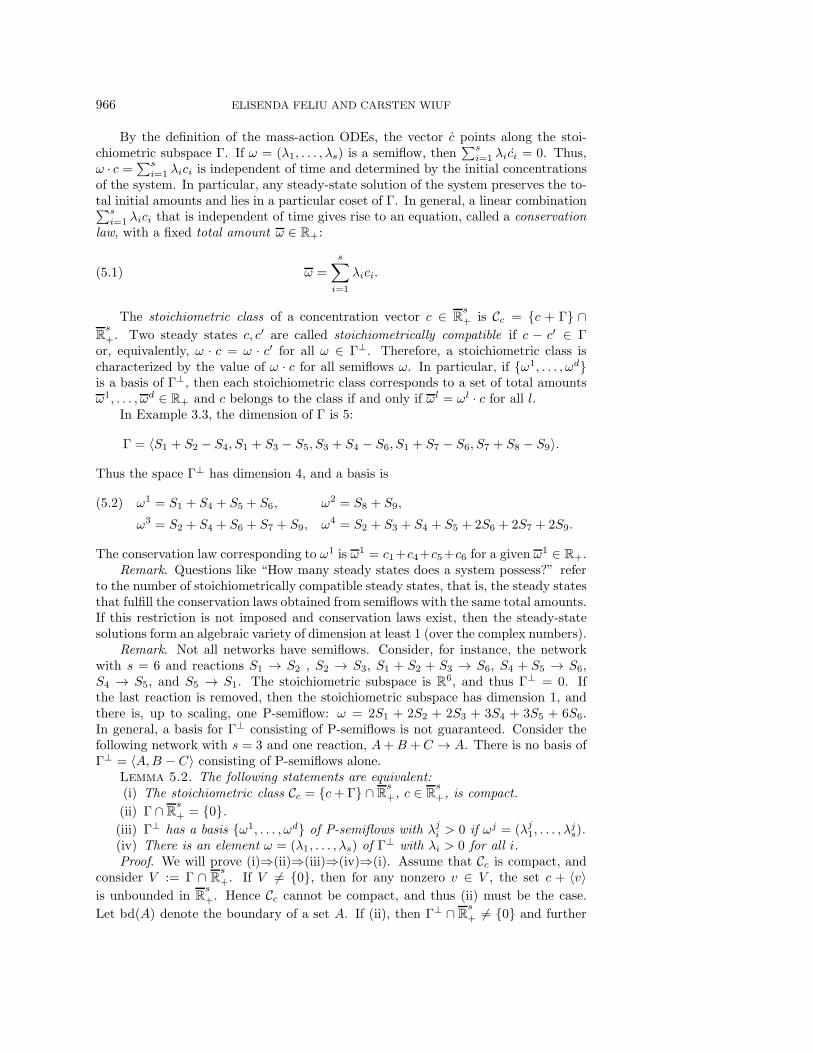
This system represents a two substrate enzyme catalysis with unordered substratebinding [12] in which S1 is an enzyme, S2, S3 are substrates, S4, S5, S6 are interme-diate enzyme-substrate complexes, and S7 is considered the product of the reactionsystem. The product dissociates via catalysis by an enzyme S8 and the formationof an intermediate complex S9. The stoichiometric coefficients of all species that arepart of a complex are one. The complex S2 + S3 + S8 involves S2, S3, S8, and its

vector expression is (0, 1, 1, 0, 0, 0, 0, 1, 0) ∈ R9+. The species S3 and S4 interact. The

complex S1 + S3 reacts to the complex S5, implying that species S1 produces speciesS5. Also, the complex S3 + S4 ultimately reacts to S1 + S7, and S7 + S8 ultimatelyreacts to S2 + S3 + S8. It follows that S3 ultimately produces S7 and S8.

4. Mass-action kinetics. The molar concentration of species Si at time t isdenoted by ci = ci(t). To any complex y we associate a monomial cy =

∏si=1 cyi

i . For

example, if y = (2, 1, 0, 1) ∈ R4+, then the associated monomial is cy = c2

1c2c4.We assume that each reaction r : y → y′ has an associated positive rate constant

ky→y′ ∈ R+ (also denoted kr). The set of reactions together with their associated rate


constants gives rise to a polynomial system of ODEs taken with mass-action kinetics :

ci =∑

y→y′∈Rky→y′cy(y′

i − yi), Si ∈ S.(4.1)

These ODEs describe the dynamics of the concentrations ci in time. The steadystates of the system are the solutions to the following system of polynomial equationsin c1, . . . , cs obtained by setting the derivatives of the concentrations to zero:

0 =∑

y→y′∈Rky→y′cy(y′

i − yi) for all i.(4.2)

These polynomial equations can be written as

(4.3) 0 =∑

r∈Rkrc

y(r)y′i(r) −

∑

r∈Rkrc

y(r)yi(r) for all i.

It is convenient to treat the rate constants as parameters with unspecified values,that is, as symbols (as we did in the example in the introduction). For that, let

Con = ky→y′ |y → y′ ∈ R

be the set of the symbols. Then, the equations (4.2) form a system of polynomialequations in c1, . . . , cs with coefficients in the field R(Con).

Only nonnegative solutions of the steady-state equations are biologically or chem-ically meaningful, and we focus on these only. The concept of S-positivity introducedabove will be key in what follows. Consider Example 3.3 and denote by ki the rateconstant of reaction ri. The mass-action ODEs are

c1 = −k1c1c2 + k2c4 − k3c1c3 + k4c5 + k9c6, c5 = k3c1c3 − k4c5 + k7c6 − k8c2c5,

c2 = −k1c1c2 + k2c4 + k7c6 − k8c2c5 + k12c9, c7 = k9c6 − k10c7c8 + k11c9,

c3 = −k3c1c3 + k4c5 − k5c3c4 + k6c6 + k12c9, c8 = −k10c7c8 + k11c9 + k12c9,

c4 = k1c1c2 − k2c4 − k5c3c4 + k6c6, c9 = k10c7c8 − k11c9 − k12c9.

c6 = k5c3c4 − k6c6 − k7c6 + k8c2c5 − k9c6,

Take, for instance, species S1. The only reactions that involve S1 are r1, r2, r3, r4, r9.The reactions r1, r3 involve S1 in the reactant complex, and thus the monomialscontain c1 and have negative coefficients. Similarly, r2, r4, r9 involve S1 only in theproduct complex, and thus the monomials do not include c1 and have positive coeffi-cients.

5. Conservation laws and P-semiflows. The dynamics of a network mightpreserve quantities that remain constant over time. If this is the case, the dynamicstakes place in a proper invariant subspace of Rs. Let x ·x′ denote the Euclidian scalarproduct of two vectors x, x′. If A is a set of vectors in some vector space, then 〈A〉denotes the linear span of A.

Definition 5.1. The stoichiometric subspace of a network, (S, C, R), is thefollowing subspace of Rs:

Γ = 〈y′ − y| y → y′ ∈ R〉.

A semiflow is a nonzero vector ω = (λ1, . . . ,λs) ∈ Γ⊥. If λi ≥ 0 for all i, then ω is aP-semiflow.


By the definition of the mass-action ODEs, the vector c points along the stoi-chiometric subspace Γ. If ω = (λ1, . . . ,λs) is a semiflow, then

∑si=1 λici = 0. Thus,

ω · c =∑s

i=1 λici is independent of time and determined by the initial concentrationsof the system. In particular, any steady-state solution of the system preserves the to-tal initial amounts and lies in a particular coset of Γ. In general, a linear combination∑s

i=1 λici that is independent of time gives rise to an equation, called a conservationlaw, with a fixed total amount ω ∈ R+:

(5.1) ω =s∑

i=1

λici.

The stoichiometric class of a concentration vector c ∈ Rs+ is Cc = c + Γ ∩

Rs+. Two steady states c, c′ are called stoichiometrically compatible if c − c′ ∈ Γ

or, equivalently, ω · c = ω · c′ for all ω ∈ Γ⊥. Therefore, a stoichiometric class ischaracterized by the value of ω · c for all semiflows ω. In particular, if ω1, . . . ,ωdis a basis of Γ⊥, then each stoichiometric class corresponds to a set of total amountsω1, . . . ,ωd ∈ R+ and c belongs to the class if and only if ωl = ωl · c for all l.

In Example 3.3, the dimension of Γ is 5:

Γ = 〈S1 + S2 − S4, S1 + S3 − S5, S3 + S4 − S6, S1 + S7 − S6, S7 + S8 − S9〉.

Thus the space Γ⊥ has dimension 4, and a basis is

ω1 = S1 + S4 + S5 + S6, ω2 = S8 + S9,(5.2)

ω3 = S2 + S4 + S6 + S7 + S9, ω4 = S2 + S3 + S4 + S5 + 2S6 + 2S7 + 2S9.

The conservation law corresponding to ω1 is ω1 = c1+c4+c5+c6 for a given ω1 ∈ R+.Remark. Questions like “How many steady states does a system possess?” refer

to the number of stoichiometrically compatible steady states, that is, the steady statesthat fulfill the conservation laws obtained from semiflows with the same total amounts.If this restriction is not imposed and conservation laws exist, then the steady-statesolutions form an algebraic variety of dimension at least 1 (over the complex numbers).

Remark. Not all networks have semiflows. Consider, for instance, the networkwith s = 6 and reactions S1 → S2 , S2 → S3, S1 + S2 + S3 → S6, S4 + S5 → S6,S4 → S5, and S5 → S1. The stoichiometric subspace is R6, and thus Γ⊥ = 0. Ifthe last reaction is removed, then the stoichiometric subspace has dimension 1, andthere is, up to scaling, one P-semiflow: ω = 2S1 + 2S2 + 2S3 + 3S4 + 3S5 + 6S6.In general, a basis for Γ⊥ consisting of P-semiflows is not guaranteed. Consider thefollowing network with s = 3 and one reaction, A+ B + C → A. There is no basis ofΓ⊥ = 〈A, B − C〉 consisting of P-semiflows alone.

Lemma 5.2. The following statements are equivalent:(i) The stoichiometric class Cc = c + Γ ∩ Rs

+, c ∈ Rs+, is compact.

(ii) Γ ∩ Rs+ = 0.

(iii) Γ⊥ has a basis ω1, . . . ,ωd of P-semiflows with λji > 0 if ωj = (λj

1, . . . ,λjs).

(iv) There is an element ω = (λ1, . . . ,λs) of Γ⊥ with λi > 0 for all i.Proof. We will prove (i)⇒(ii)⇒(iii)⇒(iv)⇒(i). Assume that Cc is compact, and

consider V := Γ ∩ Rs+. If V &= 0, then for any nonzero v ∈ V , the set c + 〈v〉

is unbounded in Rs+. Hence Cc cannot be compact, and thus (ii) must be the case.

Let bd(A) denote the boundary of a set A. If (ii), then Γ⊥ ∩ Rs+ &= 0 and further


Γ⊥ ∩ Rs+ &⊆ bd(Rs

+). If the latter were not the case, then also Γ ∩ bd(Rs+) &= 0,

contradicting (ii). Hence, there exists an open set Ω ⊆ Γ⊥ ∩ Rs+ in Γ⊥, and we can

choose a basis ω1, . . . ,ωd of P-semiflows with ωj ∈ Ω, that is, λji > 0. Thus (iii)

is fulfilled. (iii) gives (iv) directly. Assume (iv). For x = (xi)i ∈ Cc, ω · x = ω · c isindependent of x. Since λi > 0 and xi ≥ 0, xi ≤ (ω · c)/λi for all i, and thus Cc isbounded. Since it is a closed set, Cc is compact and (i) is proven.

Lemma 5.2 is well known in dynamical systems theory and Petri Net theory. Inthe latter semiflows are known as P-invariants (place invariants) [31]. The equivalencebetween (i) and (iv) in the context of chemical reaction networks was shown in [27,App. 1].

Remark. All conservation laws might not be obtained from semiflows [20], thatis, the semiflows in Γ⊥ might not give the minimal affine space in which the dynamicsof the system takes place. There can be additional conservation laws depending onthe rate constants and not merely on the stoichiometric coefficients. The next lemmais proven in [20] and stated here for future reference.

Lemma 5.3 (see [20, section 6]). If each linkage class contains exactly one ter-minal strong linkage class, then all conservation laws correspond to semiflows.

As shown in [20], any weakly reversible network fulfills the condition of the lemma.Also, Example 3.3 fulfills the criterion. The network with reactions r1 : S1 → S2,r2 : S1 → S3, and r3 : S2+S3 → 2S1 does not fulfill it [10]. Here, Γ⊥ = 〈S1+S2+S3〉,providing the conservation law c1 + c2 + c3 = ω. However, when k1 = k2 = k3, thenc1 + 2c2 is also conserved, because c2 = c3.

Minimal and terminal semiflows.Definition 5.4. The support of a semiflow ω = (λ1, . . . ,λs) is the set S(ω) =

Si| λi &= 0. We say that ω is(i) minimal if, for any semiflow ω with S(ω) ⊆ S(ω), there is a ∈ R such that

aω = ω.(ii) terminal if any semiflow ω with S(ω) ⊆ S(ω) satisfies S(ω) = S(ω).That is, a semiflow ω is minimal if any semiflow given by a linear combination of

the species in its support is a multiple of ω and terminal if there is no semiflow withsmaller support.

Lemma 5.5.(i) A semiflow is minimal if and only if it is terminal.(ii) If ω is a P-semiflow that is not minimal, then there is a P-semiflow ω such

that S(ω) ! S(ω).Proof. (i) If ω is a minimal semiflow, then by definition any semiflow ω with

S(ω) ⊆ S(ω) satisfies ω = aω for some a ∈ R. Thus, S(ω) = S(ω), which impliesthat ω is terminal. To prove the reverse, assume that ω is terminal but not minimal;that is, there exists ω such that S(ω) = S(ω) and ω &= aω for all a ∈ R. Let

I = i|Si ∈ S(ω), ω = (λ1, . . . ,λs), and ω = (λ1, . . . , λs). Choose u ∈ I such that

|λu/λu| ≥ |λi/λi| for all i ∈ I, and define γ = λu and γ = λu. Then

ω := γω − γω =s∑

i=1

(λuλi − λuλi)Si =s∑

i=1

µiSi

is a semiflow, since ω &= 0 (otherwise ω = aω for some a). Since µu = 0, S(ω) ! S(ω),which contradicts that ω is terminal.

(ii) If ω is a P-semiflow that is not minimal, then there exists a semiflow ω suchthat S(ω) ! S(ω). The construction above provides a new semiflow ω. Since λi > 0


for all i ∈ I, we have |λu|λi − λu|λi| ≥ 0 and either λu > 0 and µi ≥ 0 for all i or

λu < 0 and µi ≤ 0 for all i. Hence, either ω or −ω is a P-semiflow fulfilling (ii).Therefore, there cannot exist two linearly independent minimal P-semiflows with

the same support. For example, if S1 + S2 + S3 is conserved and minimal, thenλ1S1 + λ2S2 + λ3S3 with λ1 &= λ2 cannot be a semiflow. We will see below thatthe P-semiflows ω1,ω2,ω3 in (5.2) of Example 3.3 are minimal. However, ω4 is notminimal since S(ω3) ! S(ω4).

6. The species graph. Given a network (S, C, R), we define the species graphGS as the labeled directed graph with node set S and a directed edge from Si to Sj

with label r : y → y′ whenever yi &= 0 and y′j &= 0 for some reaction r in R. That

is, there is a directed edge from Si to Sj if and only if Si produces Sj . There canbe multiple edges with different labels between a pair of nodes. In addition, if Si

is involved both in the reactant and product of a reaction, then there is a self-edgeSi → Si. The species graph of Example 3.3 is depicted in Figure 6.1.

The species graph does not characterize a network uniquely, since informationcoming from the stoichiometric coefficients is ignored. For instance, the following twonetworks have the same species graph:

(6.1) R1 = A + B → 2C, C → A, R2 = A + B → C, C → A.

Remark. A reaction r : y → y′ is called reversible if the reaction y′ → y alsobelongs to the network. In Example 3.3, all reactions but r9, r12 are reversible. Incontrast to other papers [3, 35], we consider reversible reactions as two (independent)irreversible reactions. Thus, reversible reactions provide two edges with opposite di-rections and different labels in the species graph. This is required when we considerspanning trees in section 8. Changing a reaction from reversible to irreversible doesnot change the stoichiometric subspace, and a system with all reactions consideredirreversible has the same (P-)semiflows as a system with some (all) reactions consid-ered reversible. However, the number of steady states and their values may dependon whether reactions are reversible or not.

Definition 6.1. A graph G with node set Sα is a subgraph of GS if Sα ⊆ S andthe labeled directed edges of G are inherited from GS . We denote G = GSα . Further:

(i) Sα is full if any reaction involving some Si ∈ Sα appears at least once as alabel of an edge in GSα . If this is the case, then GSα is said to be full.

(ii) Sα is noninteracting if it contains no pair of interacting species and all stoi-chiometric coefficients are either 0 or 1, that is, yi = 0, 1 for all Si ∈ Sα and

S1 S6 S7 S9 S8

S4 S2

S5 S3

r9 r9

r12

r12

r3

r4

r4

r3

r 1

r 2

r2

r1

r 7

r 8

r6

r5r 8

r 7

r5

r6

r10

r11

r11

r10

r12

Fig. 6.1. Species graph of Example 3.3.


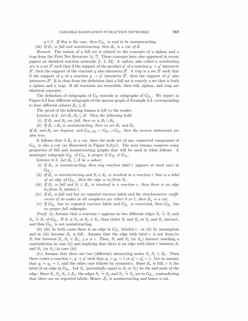
y ∈ C. If this is the case, then GSα is said to be noninteracting.(iii) If Sα is full and noninteracting, then Sα is a cut of S.Remark. The notion of a full set is related to the concepts of a siphon and a

trap from the Petri Net literature [4, 7]. These concepts have also appeared in recentpapers on chemical reaction networks [1, 2, 34]. A siphon, also called a semilockingset, is a set S ′ such that if the support of the product y′ of a reaction y → y′ intersectsS ′, then the support of the reactant y also intersects S ′. A trap is a set S ′ such thatif the support of y of a reaction y → y′ intersects S ′, then the support of y′ alsointersects S ′. It is clear from the definition that a full set is exactly a set that is botha siphon and a trap. If all reactions are reversible, then full, siphon, and trap areidentical concepts.

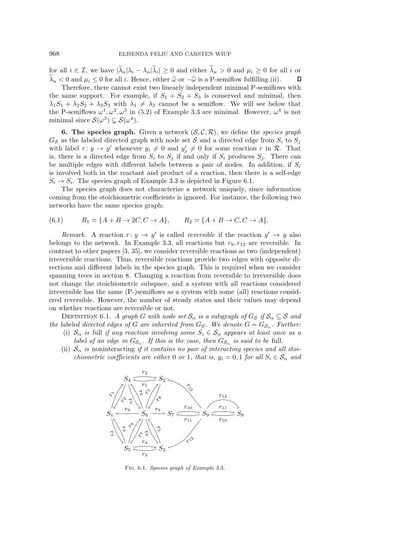
The definition of subgraphs of GS extends to subgraphs of GSα . We depict inFigure 6.2 four different subgraphs of the species graph of Example 3.3, correspondingto four different subsets Sα ⊆ S.

The proof of the following lemma is left to the reader.Lemma 6.2. Let S1, S2 ⊆ S. Then the following hold:(i) If S1 and S2 are full, then so is S1 ∪ S2.(ii) If S1 ∪ S2 is noninteracting, then so are S1 and S2.

If S1 and S2 are disjoint, and GS1∪S2 = GS1 ∪ GS2 , then the reverse statements arealso true.

It follows that if Sα is a cut, then the node set of any connected component ofGSα is also a cut (as illustrated in Figure 6.2(a)). The next lemma connects someproperties of full and noninteracting graphs that will be used in what follows. Anonempty subgraph GS′

αof GSα is proper if GS′

α&= GSα .

Lemma 6.3. Let Sα ⊆ S be a subset.(i) If Sα is noninteracting, then any reaction label r appears at most once in

GSα .(ii) If Sα is noninteracting and Si ∈ Sα is involved in a reaction r that is a label

of an edge of GSα , then the edge is to/from Si.(iii) If Sα is full and Si ∈ Sα is involved in a reaction r, then there is an edge

to/from Si labeled r.(iv) If Sα is full and has no repeated reaction labels and the stoichiometric coeffi-

cients of its nodes in all complexes are either 0 or 1, then Sα is a cut.(v) If GSα has no repeated reaction labels and GSα is connected, then GSα has

no proper full subgraphs.Proof. (i) Assume that a reaction r appears in two different edges Si

r−→ Sj and

Sur−→ Sv of GSα . If Si &= Su or Sj &= Sv, then either Si and Su or Sj and Sv interact,

and thus GSα is not noninteracting.(ii)–(iii) In both cases there is an edge in GSα labeled r—in (ii) by assumption

and in (iii) because Sα is full. Assume that the edge with label r is not from/toSi but between Sj , Su ∈ Sα, j, u &= i. Then, Si and Sj (or Su) interact reaching acontradiction in case (ii) and implying that there is an edge with label r between Si

and Su (or Sj) in case (iii).(iv) Assume that there are two (different) interacting nodes Si, Sj ∈ Sα. Then

there exists a reaction r : y → y′ such that yi = yj = 1 or y′i = y′

j = 1. Let us assumethat yi = yj = 1, and the other case follows by symmetry. Since Sα is full, r is thelabel of an edge in GSα . Let Su (potentially equal to Si or Sj) be the end node of the

edge. Since Si, Sj , Su ∈ Sα, the edges Sir−→ Su and Sj

r−→ Su are in GSα , contradictingthat there are no repeated labels. Hence, Sα is noninteracting and hence a cut.


S1 S6 S7 S9 S8

S4 S2

S5 S3

r9

r3

r4

r 1

r 2r 8

r 7

r5

r6

r11

r10

r12

(a) S1α = S1, S4, S5, S6, S8, S9

S1 S6 S7 S9 S8

S4 S2

S5 S3

r9

r12

r2

r1

r 7

r 8r5

r6

r10

r11

(b) S2α = S2, S4, S6, S7, S9

S1 S6 S7 S9 S8

S4 S2

S5 S3

r9

r 8r 7

r5

r6

r10

r11

(c) S3α = S4, S5, S6, S7, S9

S1 S6 S7 S9 S8

S4 S2

S5 S3

r9r12

r12

r4

r3

r2

r1

r 7

r 8

r6

r5

r 8r 7

r5

r6

r10

r11

(d) S4α = S2, S3, S4, S5, S6, S7, S9

Fig. 6.2. Species subgraphs of Example 3.3. The node sets in (a) and (b) are cuts, but the graphin (a) has two connected components, and the graph in (b) one; (c) the node set is noninteractingbut not full and cannot be extended to a cut; (d) is a full graph but two of its nodes, S2, S3, interact.

(v) Assume that there is a proper subgraph G. Since GSα is connected, one canfind a node Si in GSα that is not in G and a node Sj in G for which there is an edge

Sir−→ Sj or Sj

r−→ Si in GSα . By assumption a label appears at most once in GSα .Thus G is not full since r is not a label of an edge in G, but r involves Sj ∈ G.

It follows from Lemma 6.3(i), (iii) that if Sα is a cut, then all reactions involvingSi ∈ Sα label edges of GSα to/from Si, and they appear exactly once. From (i),(v) we find that noninteracting connected graphs have no proper full subgraphs. Inparticular, if Sα is a cut such that GSα is connected, then GSα has no proper fullsubgraphs.

7. Semiflows and the species graph. In this section we explore the relation-ship between semiflows, P-semiflows, and full subgraphs of GS . We come to the mainresults on semiflows in relation to variable elimination: (1) if the support of a semiflowis a cut and the associated species graph is connected, then all nonzero coefficients ofthe semiflow are equal; (2) the support of a semiflow is noninteracting if and only ifit is a cut.

Lemma 7.1. Let ω be a semiflow.(i) If ω is minimal, then GS(ω) is connected.(ii) If ω is a P-semiflow or S(ω) is noninteracting, then GS(ω) is full.(iii) If ω is a P-semiflow or S(ω) is noninteracting, and GS(ω) has no proper full

subgraphs, then ω is minimal.Proof. (i) The idea is that if GS(ω) is not connected, then the semiflow splits into

two, contradicting minimality. If GS(ω) is not connected, then GS(ω) = G1 ∪G2 withG1, G2 being two nonempty disjoint subgraphs of GS(ω). Let S1, S2 be the node setsof G1, G2, respectively. If ω =

∑si=1 λiSi, let ωk =

∑i|Si∈Sk

λiSi &= 0, k = 1, 2. SinceS1 ∩S2 = ∅, ω = ω1 +ω2. By hypothesis, ω · (y′ − y) = 0 for all y → y′ ∈ R, and thus0 = ω1 · (y′ − y) + ω2 · (y′ − y). Since G1, G2 are disjoint, there is no edge between a


node in S1 and a node in S2. If y → y′ is a reaction with y′i− yi &= 0 for some Si ∈ S1,

then yj = y′j = 0 for all Sj ∈ S2 and trivially ω2 · (y′ − y) = 0. Thus ω1 · (y′ − y) = 0.

By symmetry, we have that ω1 · (y′ − y) = ω2 · (y′ − y) = 0 for all reactions y → y′,and hence ωk is a semiflow for k = 1, 2.

(ii) Let Si ∈ S(ω) and r : y → y′ be a reaction with either yi or y′i &= 0. We

assume that yi &= 0, and the other case follows by symmetry. We want to show that ris a label in GS(ω), that is, y′

j &= 0 for some Sj ∈ S(ω). By hypothesis, ω · (y′− y) = 0.If ω = (λ1, . . . ,λs) is a P-semiflow (that is, λi ≥ 0), we have ω · y′ = ω · y ≥ λiyi > 0.If S(ω) is noninteracting, then yj = 0 for any i &= j such that Sj ∈ S(ω), and henceω · y′ = ω · y = λiyi &= 0. In either case λjy′

j &= 0 for some j, and hence y′j &= 0 for

some Sj ∈ S(ω). Note that the case j = i is accepted.(iii) Assume that ω is not minimal. Then by Lemma 5.5(i) there exists a semiflow

ω such that S(ω) ! S(ω). If ω is a P-semiflow, then by Lemma 5.5(ii) we can assumethat ω is a P-semiflow. If S(ω) is noninteracting, then so is S(ω). Using (ii), GS(ω)

is full and thus a proper full subgraph of GS(ω), which is a contradiction.Consider the P-semiflows ωi (5.2) of Example 3.3 and the subsets Si

α in Figure 6.2.Here, S(ω1) ∪ S(ω2) = S1

α, S(ω3) = S2α and S(ω4) = S4

α, giving full subgraphs. Thetwo components of GS1

αand the graph GS2

αhave no proper full subgraphs, while GS2

α

is a proper full subgraph of GS4α. Thus, it follows from Lemma 7.1(iii) that ω1,ω2,ω3

are minimal.Lemma 7.1(iii) cannot be reversed. Consider, for example, the network R2 in

(6.1). The vector ω = A+B+C is a minimal P-semiflow. The associated species graph

GS(ω) is Ar1 !! Cr2

"" Br1"" and has a proper full subgraph A

r1 !! Cr2

"" . Further,

ω2 = A+C is a P-semiflow for the network R1 in (6.1), but there is not a P-semiflowinvolving all species. This implies that if G is a full connected subgraph of G and Gcorresponds to a P-semiflow, then G does not necessarily correspond to a P-semiflow.Similarly, if G corresponds to a P-semiflow, then G does not necessarily correspondto one.

Proposition 7.2. Let Sα ⊆ S be a subset. If Sα is a cut, then ω =∑

i|Si∈SαSi

is a P-semiflow. In this case, ω is minimal if and only if GSα is connected.Proof. The stoichiometric coefficients of Si ∈ Sα are either 0 or 1 since Sα is a

cut. Consider r : y → y′ ∈ R. If yi, y′i = 0 for all i such that Si ∈ Sα, then clearly

ω · (y′− y) = 0. Since Sα is noninteracting, if yi &= 0 for some Si ∈ Sα, then yj = 0 forall Sj ∈ Sα such that i &= j. From Lemma 6.3(ii), (iii), r is the label of exactly oneedge of GSα connected to Si, and there exists exactly one species Sj ∈ Sα such thaty′j &= 0. Thus, ω · (y′ − y) = y′

j − yi = 1− 1 = 0. This shows that ω is a P-semiflow.For the second part of the statement, Lemma 7.1(i) implies that if ω is minimal,

then GSα is connected. On the other hand, if GSα is connected, then by Lemma 6.3(i),(v), GSα has no proper full subgraphs, and by Lemma 7.1(iii), ω is minimal.

The reverse is not true: In the reaction system S1 + S2 → Y1 + Y2, S3 → S1,Y1 → S3, Y2 → S3, the vector ω = S1 + S3 + Y1 + Y2 is a P-semiflow, but the setS1, S3, Y1, Y2 is not a cut. Further, ω is minimal. Thus, the noninteracting propertycannot be read from the coefficients of the P-semiflow.

Remark. If Sα is a cut, we denote the P-semiflow given in Proposition 7.2 byω(Sα) =

∑i|Si∈Sα

Si. The operation ω(·) defines a map between the set of cutsand the set of P-semiflows such that sets with connected associated species graphsare mapped to minimal P-semiflows. The operation S(·) defines a map between theset of P-semiflows and the subsets of S with full associated species graphs such that


minimal P-semiflows are mapped to subsets with connected associated species graphs.The map S(ω(·)) is the identity.

From Lemma 7.1(ii) and Proposition 7.2 we derive the following corollary.Corollary 7.3.(i) Let ω be a semiflow such that S(ω) is noninteracting. Then S(ω) is a cut.(ii) If Sα ⊆ S is a noninteracting subset and ω(Sα) is not a P-semiflow, then Sα

is not a cut, and there is no semiflow with support Sα.Therefore, there is a one-to-one correspondence between cuts and P-semiflows

with noninteracting support and nonzero entries equal to one. The results of thissection give rise to the following corollary.

Corollary 7.4. Let Sα be a noninteracting set such that GSα is connected.(i) If Sα is a cut, then any semiflow with support included in Sα is a multiple of

ω(Sα).(ii) If Sα is not a cut, then there are no semiflows with support included in Sα.Proof. Part (i) follows from Proposition 7.2 and Lemma 5.5. Part (ii) follows

from Lemma 6.3(i), (v), Lemma 7.1(ii), and the fact that GSα is not full.Consider the noninteracting subset S3

α of Example 3.3. The vector ω = S4+S5+S6 + S7 + S9 is not a P-semiflow since ω · (S1 + S2 − S4) = −1 &= 0. It follows thatS3α is not a cut and there is no semiflow with support included in S3

α. Reciprocally,consider the P-semiflow ω1. Since S1

α = S(ω1) is noninteracting, it is a cut. Further,since the graph GS2

αis connected and S2

α is a cut, any semiflow involving the speciesin S2

α is a multiple of ω3. Checking if a set is noninteracting is easy from the set ofcomplexes. However, checking that the associated species subgraph is full is in generalnot straightforward. We have shown that the relationship between semiflows and cutsgives simple conditions for determining if a noninteracting set is a cut.

Remark. Using Lemma 6.2, we find that if Sα is a cut but GSα is not connected,then Sα decomposes into a disjoint union of cuts, Sα = S1

α ∪ · · · ∪ Srα, such that GSi

α

is connected for all i. Thus, ω(Sα) = ω(S1α) + · · ·+ ω(Sr

α), and the P-semiflow ω(Sα)decomposes into a sum of minimal P-semiflows. Further, if GSα is not connected, e.g.,has two connected components GS1

αand GS2

α, then ω(S1

α)− ω(S2α) is a semiflow with

support in Sα = S1α ∪ S2

α, but it is not a multiple of ω(Sα). It follows that requiringGSα to be connected is a necessary condition in Corollary 7.4.

Remark. Note that Lemma 7.1(ii) implies that the support of a P-semiflow isalways a full set (that is, a set that is both a siphon and a trap). We have shown thatif a full set is noninteracting, then it is the support of a P-semiflow. The existence ofP-semiflows with support in a given full set can be used to prove results about thepersistence of a network [2].

8. Elimination of variables. Let Sα ⊆ S be a noninteracting subset. LetGSα be the species graph associated to Sα, and assume that it is connected. ByCorollary 7.4, either Sα is a cut and ω(Sα) is minimal, or Sα is not a cut and thereis no semiflow with support included in Sα. In what follows we discuss conditionssuch that the concentrations of the species in Sα can be fully eliminated from thesteady-state equations. The discussion depends on whether Sα is a cut or not.

For simplicity, we assume that Sα = S1, . . . , Sm. Let Rcα be the set of reactions

not appearing as labels in GSα but involving some Si ∈ Sα, and Rcα,out(i), Rc

α,in(i) thesets of reactions in Rc

α involving Si ∈ Sα in the reactants and products, respectively.Clearly, Rc

α =⋃m

i=1 Rcα,out(i) ∪Rc

α,in(i). Note that Rcα = ∅ if and only if Sα is a cut.

We restrict our attention to the steady-state equations (4.2) for a fixed Si ∈ Sα.Using the expression in (4.3) and the fact that the stoichiometric coefficients are 1,


we can write this equation as Si = Xi − Yi with

Xi =m∑

j=1j )=i

∑

Sjr−→Si

krcy(r)+

∑

r∈Rcα,in(i)

krcy(r), Yi =

m∑

j=1j )=i

∑

Sir−→Sj

krcy(r)+

∑

r∈Rcα,out(i)

krcy(r),

where the first summand in each term is taken over the edges in GSα . Recall thatthere can be more than one edge between two species. Further, since the stoichiometriccoefficient of Si is 0 or 1, any edge Si → Si provides no summand in the steady-stateequations (4.2).

Let Cα = C(Sα) = ci|Si ∈ Sα = c1, . . . , cm. Each of the monomials cy(r)

in Yi involves ci, and if another ck is involved, then Sk interacts with Si (and, inparticular, k /∈ 1, . . . , m). Similarly, cy(r) in Xi involves the variable ck if and onlyif Sk produces Si. Further, for r ∈ Rc

α,in(i), cy(r) does not involve any ck ∈ Cα,

while if r is the label of Sjr−→ Si with Sj ∈ Sα, then the only variable from Cα

involved in cy(r) is cj . It follows that the system is linear in Cα with coefficients inR[Con∪Cc(Sα)], where

(8.1) Cc(Sα) = ci|Si ∈ S \ Sα interacts with or produces some Sj ∈ Sα.

We write Ccα = Cc(Sα) for short and note that Cα ∩ Cc

α = ∅. Let yj(r) denote thevector in Rs−1 obtained from y(r) by removing the jth coordinate. We have shownthat Xi, Yi can be written so that (4.2) for Si ∈ Sα becomes

(8.2) 0 =m∑

j=1

ai,jcj + zi,

where ai,i = ei + di and

ei = −m∑

j=1j )=i

∑

Sir−→Sj

krcyi(r), ai,j =

∑

Sjr−→Si

krcyj(r),

di = −∑

r∈Rcα,out(i)

krcyi(r), zi =

∑

r∈Rcα,in(i)

krcy(r).

Let A = ai,j be the m×m matrix with ai,j defined as above, d = (d1, . . . , dm), andz = (z1, . . . , zm). Note that Sα is a cut if and only if z = d = 0. The discussion aboveprovides a proof of the following lemma.

Lemma 8.1. Let Sα ⊆ S be a noninteracting set. The steady-state equations(4.2) for Si ∈ Sα form an m×m linear system of equations in Cα, Ax+ z = 0, wherethe entries of the matrix A and the independent term z are either zero or S-positive inR[Con∪Cc

α]. Further, Sα is a cut if and only if z = d = 0, in which case the systemis homogeneous.

If A has maximal rank m, then the system has a unique solution in R(Con∪Ccα).

By Corollary 7.4, if Sα is a cut, then the column sums of A are all zero, and thesystem cannot have maximal rank. If Sα is not a cut, then there are no semiflowswith support in Sα. The column sums of the matrix A are (for column i)

m∑

k=1

ak,i =∑

i)=k

∑

Sir−→Sk

krcyi(r) −

m∑

j=1j )=i

∑

Sir−→Sj

krcyi(r) + di = di.


These are zero as polynomials in R[Con∪Ccα] if and only if Rc

α,out(i) = ∅ for all i,and the condition d = 0 is equivalent to the column sums being zero. If Sα is nota cut, but d = 0, then z &= 0 as a tuple with entries in R[Con∪Cc

α]. It follows thatthe system is incompatible in R(Con∪Cc

α), because∑

i zi &= 0. The only possiblenonnegative steady-state solutions must satisfy zi = 0 for some i and hence cj = 0for some cj ∈ Cc

α such that Sj produces Si ∈ Sα.We proceed now to discuss the case in which Sα is a cut and the case in which it

is not a cut. Both cases could be merged into a single approach, but the discussionof the first situation becomes more transparent when it is treated separately.

Elimination of variables in a cut. Let Sα ⊆ S be a cut such that GSα isconnected. For Si ∈ Sα the equations (4.2) form an m × m homogeneous linearsystem of equations with variables Cα and coefficients in R[Con∪Cc

α]. Using (8.2),the steady-state equations (4.2) become

(8.3) 0 =m∑

j=1

ai,jcj , i = 1, . . . , m.

Because the column sums of A are zero, A is the Laplacian of a labeled directed

graph GSα with node set Sα and a labeled edge Sjai,j−−→ Si whenever ai,j &= 0, i &= j.

Note that ai,j ∈ R[Con∪Ccα] is S-positive. We have that GSα is (strongly) connected

if and only if GSα is. The two graphs differ in the labels and in that multiple directededges from Si to Sj in GSα are collapsed to a single directed edge in GSα . Further,

the graph GSα has no self-loops (that is, those of GSα are removed by construction).By the Matrix-Tree theorem, the minors A(i,j) of A = L(GSα) are

A(i,j) = (−1)m−1+i+j∑

τ∈Θ(Sj)

π(τ).

Thus, A has rank m − 1 if and only if there exists at least one spanning tree in GSα

rooted at some Sj , j = 1, . . . , m. The next proposition follows from the discussion

above. In particular, the proposition holds if GSα (or, equivalently, GSα) is stronglyconnected.

Proposition 8.2. Assume that Sα is a cut such that GSα is connected, andlet ω =

∑mi=1 ci be the conservation law obtained from the P-semiflow ω(Sα). The

following statements are equivalent:(i) ω =

∑mi=1 ci is, up to scaling, the only conservation law with variables in Cα.

(ii) GSα has at least one rooted spanning tree.(iii) The rank of A is m − 1.Since GSα is connected and Sα is a cut, any semiflow with support in Sα is a

multiple of ω(Sα). The proposition says that GSα has a rooted spanning tree if andonly if there are no other conservation laws with concentrations only in Cα.

Remark. Let Sα, GSα be as in the proposition above. Let Cα be the set ofcomplexes involving at least one species in Sα. Consider the linkage classes in Cα

given by the relation “ultimately reacts to” (Definition 3.2). If GSα has a rootedspanning tree, then the root must be in a terminal strong linkage class, because theelements in such a class cannot react to complexes outside the class. Further, using thesame reasoning, there cannot be two terminal strong linkage classes. Consequently, ifGSα has a rooted spanning tree, there is only one terminal strong linkage class. Thisremark is closely related to Lemma 5.3.


For simplicity we assume that there exists a spanning tree rooted at S1. Then,the variables c2, . . . , cm can be solved in the coefficient field R(Con∪Cc

α ∪ c1). Inparticular, using Cramer’s rule and the Matrix-Tree theorem, we obtain

(8.4) cj =(−1)j+1A(1,j)

A(1,1)=

σj(Ccα)

σ1(Ccα)

c1 = ϕj(Ccα)c1, where σj(C

cα) =

∑

τ∈Θ(Sj)

π(τ)

and j = 1, . . . , m. Since there is a spanning tree rooted at S1, it follows that σ1(Ccα)

is S-positive and σj(Ccα) is either zero or S-positive in R[Con∪Cc

α]. If the graph GSα

is strongly connected, then σj(Ccα) &= 0 for all j and any choice of root Sj could be

used instead of S1. The arguments given above and the definition of ai,j provide aproof of the following lemma.

Lemma 8.3. If ck ∈ Ccα is a variable of the function σj(Cc

α) for some j, thenthere exists Si ∈ Sα that interacts with Sk and Si ultimately produces Sj via Sα.Specifically, there is a complex y1 involving Si and Sk, and a complex y2 involvingsome species Su ∈ Sα, such that y1 reacts to y2 and Su ultimately produces Sj via Sα.

If GSα is strongly connected, then the reverse is true.The sum of the concentrations in Cα is conserved. Using the equation ω =∑m

i=1 ci, we obtain

ω = (1 + ϕ2(Ccα) + · · · + ϕm(Cc

α))c1,

where the coefficient of c1 is S-positive in R(Con∪Ccα). Thus,

c1 = ϕ1(Ccα) =

ω

1 + ϕ2(Ccα) + · · · + ϕm(Cc

α)=

ωσ1(Ccα)

σ1(Ccα) + σ2(Cc

α) + · · · + σm(Ccα)

,

with ϕ1 being an S-positive rational function in Ccα with coefficients in R(Con∪ω).

Observe that ω becomes an extra parameter and can be treated as a symbol as well.Further, if ω is assigned a positive value, then c1 > 0 at steady state for positivevalues of Cc

α. By substitution of c1 by ϕ1, we obtain

(8.5) cj = ϕj(Ccα) := ϕj(C

cα)ϕ1(C

cα), j = 2, . . . , m,

with ϕj being either zero or an S-positive rational function in Ccα with coefficients in

R(Con∪ω).If, in the discussion above, we replace the fixed species S1 by any other species

Si in Sα, we obtain the following proposition.Proposition 8.4. Let Sα ⊆ S be a cut such that GSα is connected. Assume

that there is a spanning tree of GSα rooted at some species Si for some i. Then, thereexists a zero or S-positive rational function ϕj in Cc

α with coefficients in R(Con), suchthat the steady-state equation (4.2) for cj ∈ Cα is satisfied in R(Con∪Cc

α) if and onlyif

cj = ϕj(Ccα)ci, cj ∈ Cα.

Further, there exists an S-positive rational function ϕi in Ccα with coefficients in

R(Con∪ω), such that the conservation law ω =∑m

k=1 ck is fulfilled if and onlyif ci = ϕi(C

cα).


Consider Example 3.3 and the cut Sα = S1, S4, S5, S6 corresponding to a con-nected component of the graph GS1

αin Figure 6.2(a). System (8.3) becomes

−k1c2 − k3c3 k2 k4 k9

k1c2 −k2 − k5c3 0 k6

k3c3 0 −k4 − k8c2 k7

0 k5c3 k8c2 −k6 − k7 − k9

c1

c4

c5

c6

= 0.

The column sums are zero because of the conservation law ω1 = c1 + c4 + c5 + c6.The graph GSα is strongly connected (Figure 8.1(a)), as is observed in many real(bio)chemical systems. Thus rooted spanning trees exist, and the system has rank 3.This also follows from Proposition 8.2 and Lemma 5.3, since each linkage class of thenetwork has exactly one terminal strong linkage class.

The polynomials σj are

σ1 = k2k4(k6 + k7 + k9) + k2k8(k6 + k9)c2 + k4k5(k7 + k9)c3 + k5k8k9c2c3,

σ4 = k1k4(k6 + k7 + k9)c2 + k1k8(k6 + k9)c22 + k3k6k8c2c3,

σ5 = k2k3(k6 + k7 + k9)c3 + k3k5(k7 + k9)c23 + k1k5k7c2c3,

σ6 = (k1k4k5 + k2k3k8)c2c3 + k1k5k8c22c3 + k3k5k8c2c

23.

Each monomial in σj corresponds to a spanning tree rooted at Sj. The species S2, S3

are the only species interacting with a species in Sα, and thus only c2, c3 appear in theexpressions. Using (8.4) and (8.5) we find the steady-state expressions of c1, c4, c5, c6

in terms of the rate constants, the total amount ω1, and the concentrations c2, c3.Remark. It is straightforward to find σj by computing the minors of A using

any computer algebra software. The advantage of the Matrix-Tree description in thetheoretical discussion is that S-positivity of the solutions is easily obtained.

Elimination of variables in a subset that is not a cut. Let Sα ⊆ S bea noninteracting subset that is not a cut, and assume that GSα is connected. Asdiscussed above, if the column sums of the matrix A are zero, then there are nopositive steady-state solutions. If the column sums of A are not all zero, then A isnot a Laplacian. However, A can be extended such that its determinant is a minor ofa Laplacian.

Consider the labeled directed graph GSα with node set Sα ∪ ∗. We order thenodes such that Si is the ith node and ∗ the (m + 1)th node. The graph GSα has

the following labeled directed edges: Sjai,j−−→ Si if ai,j &= 0 and i &= j, Si

−di−−→ ∗ if

di &= 0, and ∗ zi−→ Si if zi &= 0. All labels are S-positive in R[Con∪Ccα]. Let L = λi,j

be the Laplacian of GSα . If i, j ≤ m, then λi,j = ai,j . The entries of the last roware λm+1,i = −di for i ≤ m, and the entries of the last column are λi,m+1 = zi fori ≤ m. We conclude that the (m + 1, m + 1) minor of L is exactly A, and thus, bythe Matrix-Tree theorem, we have

σ(Ccα) := (−1)m det(A) = (−1)mL(m+1,m+1) =

∑

τ∈Θ(∗)

π(τ).

If there exists at least one spanning tree rooted at ∗, then (−1)m det(A) is S-positive inR[Con∪Cc

α]. In this case the system Ax+z = 0 has a unique solution in R(Con∪Ccα).

A spanning tree rooted at ∗ exists if and only if for all species Si ∈ Sα there existsa reaction y → y′ such that y′ does not involve any species in Sα, y involves some


S1 S6

S4

S5

k9

k3 c

3

k4

k1c2

k2

k8c2

k7

k5 c

3

k6

(a) Sα = S1, S4, S5, S6

S6 S7 S9

S4

S5

∗k9 k12

k8 c

2

k7

k 5c 3

k 6

k10c8

k11

k2

k1c1c2

k4

k3c1c3

(b) S2α = S4, S5, S6, S7, S9

Fig. 8.1. (a) The graph GSα in Example 3.3 for the cut Sα. (b) The graph G2Sα

for the

noninteracting set S2α, which is not a cut.

Su ∈ Sα, and Si ultimately produces Su. The existence of such a spanning treeensures that Rc

α,out(i) &= ∅ and thus di &= 0 for some i.Since A is noninteracting but not a cut, there are no semiflows with support in Sα

by Corollary 7.4(ii). Similarly to Proposition 8.2, we obtain the following proposition.Proposition 8.5. Assume that Sα is a noninteracting set that is not a cut

and such that GSα is connected. Then A has maximal rank if and only if thereexists a spanning tree rooted at ∗. Further, if A has maximal rank, then there are noconservation laws in the concentrations in Cα.

If A does not have maximal rank, then there is a vanishing linear combinationof the rows of A, 0 =

∑mk=1 λkak,j for all j. If there are no conservation laws in

the concentrations in Cα, then 0 &=∑m

k=1 λk ck =∑m

k=1

∑mj=1 λk(ak,jcj + zk), and it

follows that∑m

k=1 λkzk &= 0. If λk ≥ 0 for all k, then we conclude that the system(8.2) is incompatible in R(Con∪Cc

α) and there are no positive steady states.Assume that a spanning tree rooted at ∗ exists. For i = 1, . . . , m, let σi be the

following polynomial in Ccα:

σi(Ccα) = (−1)i+1L(m+1,i) =

∑

τ∈Θ(Si)

π(τ),

which is either zero or S-positive in R[Con∪Ccα]. By Cramer’s rule, we have

ci = ϕi(Ccα) =

(−1)m+1−iL(m+1,i)

(−1)mL(m+1,m+1)=

σi(Ccα)

σ(Ccα)

,

which is either zero or S-positive in R(Con∪Ccα). If there exists at least one spanning

tree rooted at Si, then σi &= 0 as a polynomial in R[Con∪Ccα]. A necessary condition

for σi &= 0 is the existence of a directed path from ∗ to Si, which implies that Si isultimately produced from some species Sk ∈ S \ Sα. In particular, if GSα is stronglyconnected, then all concentrations are nonzero as elements in R(Con∪Cc

α).Consider the set Sα = S3

α = S4, S5, S6, S7, S9 in Example 3.3. It is noninter-acting and not a cut, and GSα is connected. Further, all species ultimately produceS9 ∈ Sα, and S9 reacts to S2 + S3 + S8, which does not involve species in Sα. Hencea spanning tree rooted at ∗ exists. The graph GSα is depicted in Figure 8.1(b) andis strongly connected. We have that z = (k1c1c2, k3c1c3, 0, 0, 0), Cc

α = c1, c2, c3, c8,and

σ =k10k12(k2k4(k6 + k7 + k9) + k2k6k8c2


+ k4k5k7c3 + k9(k4k5c3 + k2k8c2 + k5k8c2c3))c8,

σ4 =k10k12(k1k4(k6 + k7 + k9) + k1k8(k6 + k9)c2 + k3k6k8c3)c1c2c8,

σ5 =k10k12(k2k3(k6 + k7 + k9) + k1k5k7c2 + k3k5(k7 + k9)c3)c1c3c8,

σ6 =k10k12(k1k4k5 + k2k3k8 + k1k5k8c2 + k3k5k8c3)c1c2c3c8,

σ7 =k9(k11 + k12)(k1k4k5 + k2k3k8 + k1k5k8c2 + k3k5k8c3)c1c2c3,

σ9 =k9k10(k1k4k5 + k2k3k8 + k1k5k8c2 + k3k5k8c3)c1c2c3c8.

The concentration c1 is only in the label of out-edges from ∗, and thus c1 is not in σ.Proposition 8.6. Assume that there is a spanning tree of GSα rooted at ∗. Then,

there exists a zero or S-positive rational function ϕi in Ccα with coefficients in R(Con),

such that the steady-state equations (4.2) for ci ∈ Cα are satisfied in R(Con∪Ccα) if

and only if ci = ϕi(Ccα).

Remark. The procedure outlined here can be stated in full generality: Considera square linear system of equations Ax + z = 0, such that the entries of z and theoff-diagonal entries of A are positive and the column sums of A are zero or negative.If A has maximal rank, then the unique solution of the system is nonnegative.

Remark. If the matrix A does not have maximal rank, then we can always selecta subset of Sα such that the corresponding matrix has maximal rank and proceedwith elimination of the variables in the subset.

Remarks. Let Sα ⊆ S be any noninteracting subset such that GSα is connected.We have proven that for all ci ∈ Cα there exists a rational function ϕi such thatci = ϕi(Cc

α) at steady state, provided some spanning trees exist. When Sα is a cut,the P-semiflow ω(Sα) is required in the elimination, while when Sα is not a cut,variables are eliminated using only the steady-state equations.

If GSα is not connected, then the results above apply to the connected com-ponents separately, since the underlying node set of each connected component isnoninteracting. Further, let S1

α, S2α be two noninteracting sets such that GS1

αand

GS2αare disjoint and connected. One easily sees that C(S2

α) ∩ Cc(S1α) = ∅; that is,

both sets of variables C(S1α) and C(S2

α) can be simultaneously eliminated. Addition-ally, if we let Sα = S1

α ∪ S2α, then Cc(Sα) = Cc(S1

α) ∪ Cc(S2α). For instance, consider

Sα = S1, S4, S5, S6, S8, S9 in Figure 6.2(a). The associated species graph has twoconnected components, which are strongly connected. The concentrations ci ∈ Cα

can be expressed as S-positive rational functions in Ccα = c2, c3, c7.

The conditions to apply the variable elimination procedure are summarized inTable 8.1. The procedure guarantees that if positive values are assigned to all cj ∈ Cc

α,then ci is nonnegative. For ci to be positive, that is, σi &= 0, the existence of at leastone in-edge to Si is necessary. Otherwise the concentration at steady state of Si iszero, which is expected if Si is only consumed and never produced. Further, we havethe following proposition.

Table 8.1Summary of the conditions required for the variable elimination procedure for a noninteracting

set Sα. Here “only” indicates up to multiplication by a constant.

Sα cut Sα not a cutCharacterization ω(Sα) semiflow or z = d = 0 " semiflow or z − d "= 0

Elimination of Cα

works if in GSα ...∃ rooted spanning tree (equivalentto ω =

∑ci∈Cα

ci being the “only”

conservation law in Cα)

∃ spanning tree rooted at ∗ (im-plies " conservation law in Cα andd "= 0)


Proposition 8.7. Let Sα be a noninteracting subset of S such that the con-centrations Cα can be eliminated from the steady-state equations using the proceduredescribed in this section. Each component of the graph GSα is strongly connected ifand only if any steady-state solution satisfies cj > 0 for all cj ∈ Cα (and for any pos-itive total amount if appropriate) whenever the variables in Cc

α take positive values.

9. Steady-state equations. Let Sα be any noninteracting subset such thatGSα is connected and such that the variables in Cα can be eliminated by the proce-dure above. Let Φu(Cc

α) = 0 be the equation obtained from cu = 0, u = m+1, . . . , s,after elimination of variables in Cα and removal of denominators. The denomina-tors can be chosen to be S-positive. With this choice, the denominators have nopositive zeros, and therefore multiplication by the denominators does not change thesolutions or the positivity of them. Fix a maximal set of n independent combinationsξl(c1, . . . , cs) =

∑si=1 λ

lici providing conservation laws that includes those correspond-

ing to the full connected components of GSα (that is, to cuts). For given total amounts,the steady-state equations are complemented with the equations ωl = ξl(c1, . . . , cs),l = 1, . . . , n. If the conservation law corresponds to a cut, then the eliminationprocedure ensures that ξl(ϕ1(Cc

α), . . . ,ϕm(Ccα), cm+1, . . . , cs) = ωl, and the equation

becomes redundant.Theorem 9.1. Consider a network with a noninteracting set Sα. Assume that

Sα = S1α ∪ · · · ∪ Sr

α is a partition of Sα into disjoint sets such that GSjαis connected

and GSjαadmits a spanning tree for all j. If Sj

α is a cut, assume that the spanningtree is rooted at some Si ∈ Sα, and otherwise assume that it is rooted at ∗. Let totalamounts ωl be given for the n conservation laws.

The nonnegative steady states with positive values in Ccα are in one-to-one corre-

spondence with the positive solutions to

Φu(Ccα) = 0, ωl = ξl(Cc

α) := ξl(ϕ1(Ccα), . . . ,ϕm(Cc

α), cm+1, . . . , cs)

for u = m + 1, . . . , s and l = 1, . . . , n.Proof. We have shown that any nonnegative steady-state solution with positive

values for ci ∈ Ccα must satisfy these equations. For the reverse, we apply the following

to each connected component of GSα . Consider a positive solution c = (cm+1, . . . , cs)to the equations Φu(Cc

α) = 0 and ωl = ξl(Ccα). For i = 1, . . . , m, define ci through

Proposition 8.4 or 8.6, depending on whether Si belongs to a cut Sjα or not. For posi-

tive rate constants and positive total amounts, ci is nonnegative (because the rationalfunctions defining it are S-positive). By construction this procedure automaticallyensures that conservation laws corresponding to cuts are fulfilled. Using Proposi-tions 8.4 and 8.6 the values ci satisfy (4.2). Since Φu(Cc

α) = 0 is the steady-stateequation cu = 0 after substitution of the eliminated variables, this equation is alsosatisfied, and the same reasoning applies to the equation ωl = ξl(c1, . . . , cm). Thus,(c1, . . . , cm) is a solution to the steady-state equations and satisfies the conservationlaws corresponding to the total amounts ωl.

This theorem and Proposition 8.7 together give the following corollary.Corollary 9.2. With the conditions of Theorem 9.1, assume further that each

graph GSjαis strongly connected. Then, the positive steady states of the system are in

one-to-one correspondence with the positive solutions to Φu(Ccα) = 0 and ωl = ξl(Cc

α)for u = m + 1, . . . , s and l = 1, . . . , n. Further, if a steady-state solution satisfiesci = 0 for ci ∈ Cα, then there exists some cj ∈ Cc

α such that cj = 0.In Example 3.3, the set Sα = S1, S4, S5, S6, S8, S9 is the largest noninter-

acting subset of S and thus provides the maximal number of linearly eliminated


concentrations. The initial system of steady-state equations is reduced to threeequations—for instance, the one corresponding to c7 = 0, and the two conservationlaws ω3 = c2 + c4 + c6 + c7 + c9 and ω = c3 + c5 + c6 + c7 + c9 (which corre-sponds to ω4 − ω3). Because of the conservation laws, the equations c2 = 0 andc3 = 0 are redundant. The elimination from cuts provides ck = σk/σ1 for k = 4, 5, 6,c1 = ω1σ1/(σ1+σ4+σ5+σ6), c9 = σ9/σ8, and c8 = ω2σ8/(σ8+σ9) with σi S-positivepolynomials in c2, c3, c7 and coefficients inR(Con∪ω1,ω2) for all i. The steady-stateequations are thus reduced to 0 = k9σ6(σ8 +σ9)σ8 − k10ω2σ2

8σ1c7 + k11σ1σ9(σ8 +σ9),ω3σ1σ8 = σ1σ8c2+σ4σ8+σ6σ8+σ1σ8c7+σ1σ9, and ωσ1σ8 = σ1σ8c3+σ5σ8+σ6σ8+σ1σ8c7 + σ1σ9.

Acknowledgment. Part of this work was done while the authors were visitingImperial College London in the fall of 2011.

REFERENCES

[1] D. Anderson, Global asymptotic stability for a class of nonlinear chemical equations, SIAMJ. Appl. Math., 68 (2008), pp. 1464–1476.

[2] D. Angeli, P. De Leenheer, and E. Sontag, A petri net approach to the study of persistencein chemical reaction networks, Math. Biosci., 210 (2007), pp. 598–618.

[3] D. Angeli, P. De Leenheer, and E. Sontag,Graph-theoretic characterizations of monotonic-ity of chemical networks in reaction coordinates, J. Math. Biol., 61 (2010), pp. 581–616.

[4] F. Chu and X. L. Xie, Deadlock analysis of petri nets using siphons and mathematical pro-gramming, IEEE Trans. Robotic Autom., 13 (1997), pp. 793–804.

[5] C. Conradi and D. Flockerzi, Switching in Mass Action Networks Based on Linear Inequal-ities, preprint, http://arxiv.org/abs/1002.1054v1, 2010.

[6] C. Conradi, D. Flockerzi, J. Raisch, and J. Stelling, Subnetwork analysis reveals dy-namic features of complex (bio)chemical networks, Proc. Natl. Acad. Sci. USA, 104 (2007),pp. 19175–19180.

[7] R. Cordone, L. Ferrarini, and L. Piroddi, Enumeration. algorithms for minimal siphons inpetri nets based on place constraints, IEEE Trans. Syst. Man. Cy. A, 35 (2005), pp. 844–854.

[8] A. Cornish-Bowden, Fundamentals of Enzyme Kinetics, 3rd ed., Portland Press, London,2004.

[9] G. Craciun and M. Feinberg, Multiple equilibria in complex chemical reaction networks:I. The injectivity property, SIAM J. Appl. Math., 65 (2005), pp. 1526–1546.

[10] G. Craciun and M. Feinberg, Multiple equilibria in complex chemical reaction networks:Extensions to entrapped species models, Syst. Biol. (Stevenage), 153 (2006), pp. 179–186.

[11] G. Craciun and M. Feinberg, Multiple equilibria in complex chemical reaction networks:II. The species-reaction graph, SIAM J. Appl. Math., 66 (2006), pp. 1321–1338.

[12] G. Craciun, Y. Tang, and M. Feinberg, Understanding bistability in complex enzyme-drivenreaction networks, Proc. Natl. Acad. Sci. USA, 103 (2006), pp. 8697–8702.

[13] R. Diestel, Graph Theory, 3rd ed., Grad. Texts in Math. 173, Springer-Verlag, Berlin, 2005.[14] P. Ellison, M. Feinberg, and H. Ji, Chemical Reaction Network Toolbox, available online

from http://www.chbmeng.ohio-state.edu/ feinberg/crntwin/, 2011.[15] M. Feinberg, On chemical kinetics of a certain class, Arch. Ration. Mech. Anal., 46 (1972),

pp. 1–41.[16] M. Feinberg, Lectures on Chemical Reaction Networks, available online from

http://www.chbmeng.ohio-state.edu/ feinberg/LecturesOnReactionNetworks/, 1980.[17] M. Feinberg, Chemical reaction network structure and the stability of complex isothermal

reactors I. The deficiency zero and deficiency one theorems, Chem. Eng. Sci., 42 (1987),pp. 2229–2268.

[18] M. Feinberg, The existence and uniqueness of steady states for a class of chemical reactionnetworks, Arch. Ration. Mech. Anal., 132 (1995), pp. 311–370.

[19] M. Feinberg and F. J. M. Horn, Dynamics of the open chemical systems and algebraicstructure of the underlying reaction network, Chem. Eng. Sci., 29 (1974), pp. 775–787.

[20] M. Feinberg and F. J. M. Horn, Chemical mechanism structure and the coincidence of thestoichiometric and kinetic subspaces, Arch. Ration. Mech. Anal., 66 (1977), pp. 83–97.


[21] E. Feliu and C. Wiuf, Variable elimination in post-translational modification reaction net-works with mass-action kinetics, J. Math. Biol. Online First, DOI 10.1007/s00285-012-0510-4, http://www.springerlink.com/content/11p5h78426l48151/?MUD=MP, 2012.

[22] J. L. Gross and J. Yellen, Graph Theory and Its Applications, 2nd ed., Discrete Math. Appl.,Chapman & Hall/CRC, Boca Raton, FL, 2006.

[23] J. Gunawardena, Distributivity and processivity in multisite phosphorylation can be distin-guished through steady-state invariants, Biophys. J., 93 (2007), pp. 3828–3834.

[24] J. Gunawardena, A linear framework for time-scale separation in nonlinear biochemical sys-tems, PLoS One, 7 (2012), e36321.

[25] H. A. Harrington, K. L. Ho, T. Thorne, and M. P. H. Stumpf, A Parameter-Free Model Selection Criterion Based on Steady-State Coplanarity, preprint,http://arxiv.org/abs/1109.3670, 2011.

[26] R. Heinrich, B. G. Neel, and T. A. Rapoport, Mathematical models of protein kinase signaltransduction, Mol. Cell, 9 (2002), pp. 957–970.

[27] F. J. M. Horn and R. Jackson, General mass action kinetics, Arch. Ration. Mech. Anal., 47(1972), pp. 81–116.

[28] C. Y. Huang and J. E. Ferrell, Ultrasensitivity in the mitogen-activated protein kinasecascade, Proc. Natl. Acad. Sci. USA, 93 (1996), pp. 10078–10083.

[29] A. K. Manrai and J. Gunawardena, The geometry of multisite phosphorylation, Biophys. J.,95 (2008), pp. 5533–5543.

[30] N. I. Markevich, J. B. Hoek, and B. N. Kholodenko, Signaling switches and bistabilityarising from multisite phosphorylation in protein kinase cascades, J. Cell Biol., 164 (2004),pp. 353–359.

[31] A. Marsan, G. Balbo, G. Conte, S. Donatelli, and G. Franceschinis, Modelling withGeneralized Stochastic Petri Nets, John Wiley and Sons, London, 1995.

[32] M. Perez Millan, A. Dickenstein, A. Shiu, and C. Conradi, Chemical reaction systemswith toric steady states, Bull. Math. Biol., 74 (2012), pp. 1027–1065.

[33] G. Shinar and M. Feinberg, Structural sources of robustness in biochemical reaction net-works, Science, 327 (2010), pp. 1389–1391.

[34] A. Shiu and B. Sturmfels, Siphons in chemical reaction networks, Bull. Math. Biol., 72(2010), pp. 1448–1463.

[35] M. Thomson and J. Gunawardena, The rational parameterization theorem for multisite post-translational modification systems, J. Theor. Biol., 261 (2009), pp. 626–636.

[36] W. T. Tutte, The dissection of equilateral triangles into equilateral triangles, Proc. CambridgePhilos. Soc., 44 (1948), pp. 463–482.

Documents

VARIABLE ELIMINATION IN CHEMICAL REACTION NETWORKS