Valuing Stock Options:The Black-Scholes-Merton

Model

Chapter 13

1

The Black-Scholes-Merton Random Walk Assumption

l Consider a stock whose price is S

l In a short period of time of length Δt, the return on the stock (ΔS/S) is assumed to be normal with: l mean µ Δtl standard deviation

·µ is the annualized expected return and σ is the annualized volatility.

tΔσ

2

Why can we say that?

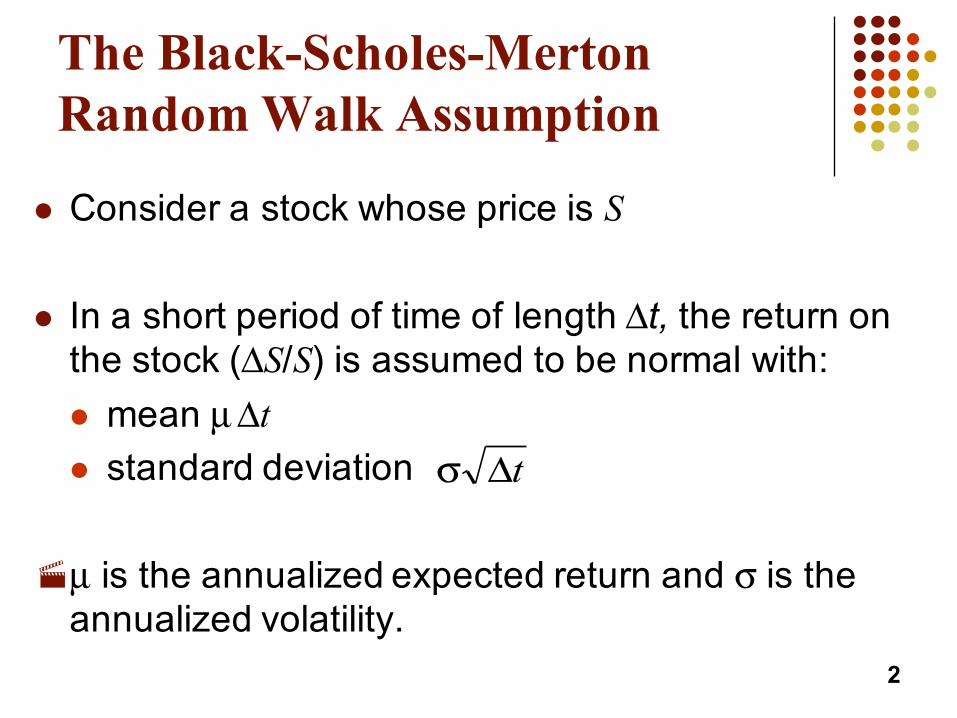
l Assume that the Normal(µ,σ2) annual return is made up of the sum of n returns of shorter horizons (eg. monthly, weekly):

l We have n=1/Δt intervals of length Δt in a year (eg. for monthly n=1/(1/12) = 12 intervals of length 1/12 of a year), therefore:

3

1 1

2 2

1 1

( ) ( ) ( ) thus ( ) /

( ) ( ) ( ) thus ( ) /

n n

i i i ii i

n n

i i i ii i

E r E r nE r E r n

Var r Var r nVar r Var r n

µ µ

σ σ

= =

= =

= = = =

= = = =

∑ ∑

∑ ∑

2 2 2

( ) / / (1/ )

( ) / / (1/ )

( )

i

i

i

E r n t tVar r n t t

Sigma r t

µ µ µσ σ σ

σ

= = Δ = Δ

= = Δ = Δ

= Δ

The Lognormal Property

l These assumptions imply that ln ST is normally(Gaussian) distributed with mean:

and standard deviation:

l Because the logarithm of ST is normal, the future value or price (at time T) of the stock ST is said to be lognormally distributed.

TS )2/(ln 20 σ−µ+

Tσ

4

Proof, if you like details… J

§ Let a security price St evolve over time according to:§ dSt /St = µ dt + σ dZt where dZt~N(0,Δt) (Δt=variance)§ Note that this also means that dSt /St = µ dt + σ N(0,1)§ Multiplying by St on both sides yields: dSt = µSt dt + σSt dZt

§ Itô’s lemma says that if f is a function of S, i.e., ft=f(St) then:§ dft = { µSt [df/dS] + (1/2)(σSt)2 [d2f/dS2] } dt + σSt [df/dS] dZt

§ If we choose f(St) = ln(St), then df/dS = 1/St and d2f/dS2 = -1/St2

§ Therefore dft = {µ – σ2/2} dt + σ dZt

§ Remembering that ft = ln(St) and integrating between time 0 and T, we get:

5

tΔ

2 2

0 0 0 02 2 2 2

02 2 2 2

0 0

ln(S ) { / 2} { / 2} (0,T)

so we have ln( ) ln( ) ({ / 2} , ) [( / 2) , ]

or ln( / S ) [( / 2) , ] or ln( ) [ln( ) ( / 2) , ]

T T T T

t t t

T

T T

df dt d dt dt dZ T N

S S N T T T TS T T S S T T

µ σ σ µ σ σ

µ σ σ φ µ σ σφ µ σ σ φ µ σ σ

= = − + = − +

− = − ≡ −

≈ − ≈ + −

∫ ∫ ∫ ∫

The Lognormal Property(continued)

where φ[m,v] is a normal distribution with mean m and variance v

[ ]

[ ]TTSS

TTSS

T

T

22

0

220

,)2(ln

,)2(lnln

σσ−µφ≈

σσ−µ+φ≈or

6

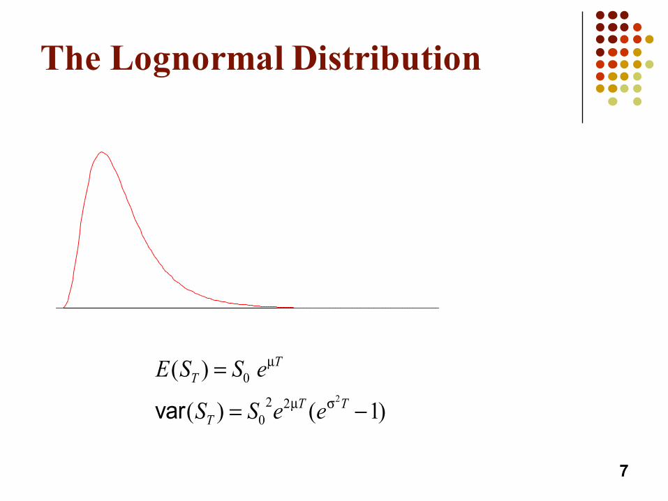
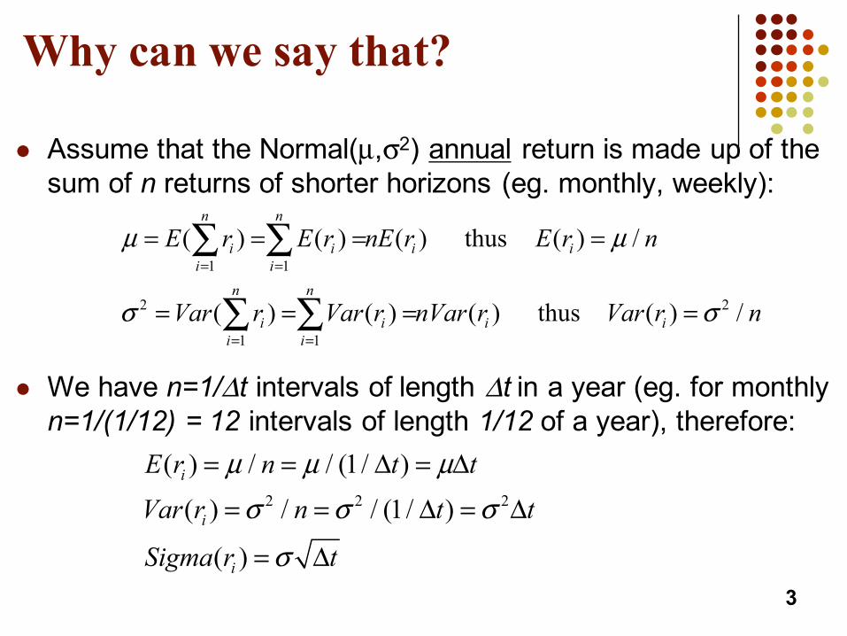
The Lognormal Distribution

E S S e

S S e eT

T

TT T

( )

( ) ( )

=

= −0

02 2 2

1

var

µ

µ σ

7

Confidence Intervals

l We know that

l The fact that the (natural) logarithm of ST is Normally distributed is useful because we can then compute probabilities of the future stock value, ST, being within a certain range of prices, below, or above a certain price.

l For example, if S0=40, T=1/2, µ=16%, and σ=20%, we have:l ln(ST) ~ N( ln(40)+(0.16-0.22/2)(1/2) , 0.22(1/2) )l Or ln(ST) ~ N( 3.759 , 0.02 )l Note that σ = (0.02)(1/2) = 0.141 (square root of the variance)

8

2 20ln ln ( 2) ,TS S T Tϕ µ σ σ⎡ ⎤≈ + −⎣ ⎦

Confidence Intervals: Going from Probabilities to Stock Prices

l Since we know that there is a 95% probability that a Normal random variable has a value within 1.96 standard deviations of its mean, we can say that, 95% of the time, we’ll have:

l 3.759 – 1.96(0.141) < ln(ST) < 3.759 + 1.96(0.141)l Or that e3.759 – 1.96(0.141) < ST < e3.759 + 1.96(0.141)

l And therefore that 32.55 < ST < 56.56

l In other words, there is a 95% probability that the stock price in six months will be between 32.55 and 56.56

9

Confidence Intervals: the Big Picture

l More generally, we can compute anything we want by taking advantage of the NORM.DIST (the older name was NORMDIST, but it still works) or NORMINV Excel functions.

l The NORMINV takes as input the cumulative probability (area under the Normal/Gaussian distribution curve up to a value x), and returns the corresponding value x.

l The NORM.DIST function takes as input a value x and returns the cumulative probability area under the Normal/Gaussian distribution curve up to that value x. It is essentially the “opposite” of NORMINV.

10

Confidence Intervals: The Big Picture

l In general, if the known/chosen input is a confidence interval probability, in order to get the corresponding stock prices, the NORMINV Excel function is needed.

l In the previous example, we could have computed directly:l eNORMINV(0.025, 3.759, 0.141) = 32.55l eNORMINV(0.975, 3.759, 0.141) = 56.56

l If, on the other hand, the known/chosen inputs are specificstock prices, in order to get the corresponding probabilities, the NORM.DIST Excel function is needed.

11

Probability of making a profit using NORM.DIST

l For example, assume that you have entered into a straddlestrategy, and you know that you will make a profit only if the stock price ends up below $40 or above $50 four months from now (recall that the payoff has a “V shape”).

l Assume that the stock has an average arithmetic return of 10%, a standard deviation of 15%, and currently trades at $43.

l What is the probability of making a profit?

12

Probability of making a profit

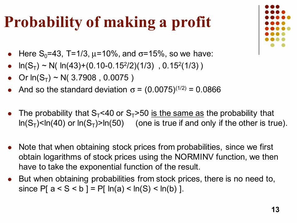
l Here S0=43, T=1/3, µ=10%, and σ=15%, so we have:l ln(ST) ~ N( ln(43)+(0.10-0.152/2)(1/3) , 0.152(1/3) )l Or ln(ST) ~ N( 3.7908 , 0.0075 )l And so the standard deviation σ = (0.0075)(1/2) = 0.0866

l The probability that ST<40 or ST>50 is the same as the probability that ln(ST)<ln(40) or ln(ST)>ln(50) (one is true if and only if the other is true).

l Note that when obtaining stock prices from probabilities, since we first obtain logarithms of stock prices using the NORMINV function, we then have to take the exponential function of the result.

l But when obtaining probabilities from stock prices, there is no need to, since P[ a < S < b ] = P[ ln(a) < ln(S) < ln(b) ].

13

Probability of making a profit

l Proba[ ln(ST)<ln(40) ] = NORM.DIST( ln(40), 3.7908, 0.0866, TRUE )l Proba[ ln(ST)>ln(50) ] = 1 - NORM.DIST( ln(50), 3.7908, 0.0866, TRUE )

(if you entered FALSE instead, the function would have returned the value of the Normal or Gaussian density function instead of the cumulative probability).

l Therefore we have:l Proba[ln(ST)<ln(40)] = .1197 or 11.97%l Proba[ln(ST)>ln(50)] = .0807 or 8.07%

l We will make a profit if either one of these scenarios comes true, thus we have a 11.97 + 8.07 = 20.04% chance of making a profit with this straddle strategy.

14

Arithmetic vs. Geometric Return

l The arithmetic average (mean) return in a short period Δt is µΔt.If Δt=1 (one year), the arithmetic average return is µ.

l This is because the return over one short period is given as: dSt /St = µ dt + σ N(0,dt)

l But over the long run, the geometric average return on the stock is closer to: µ – σ2/2.

l Recall that the future value of the stock over a longer period Tis given by ST = S0 eRT , with the rate R ~ N( µ – σ2/2 , variance).

l The geometric average return is thus analogous to the average continuously compounded return.

15

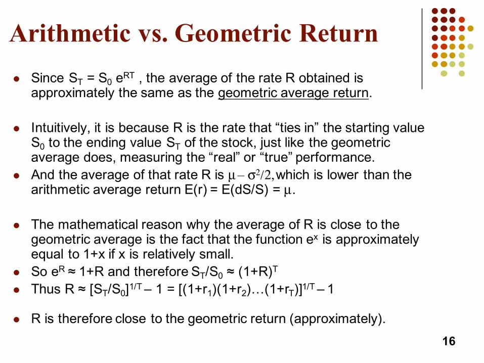
Arithmetic vs. Geometric Returnl Since ST = S0 eRT , the average of the rate R obtained is

approximately the same as the geometric average return.

l Intuitively, it is because R is the rate that “ties in” the starting value S0 to the ending value ST of the stock, just like the geometric average does, measuring the “real” or “true” performance.

l And the average of that rate R is µ – σ2/2, which is lower than the arithmetic average return E(r) = E(dS/S) = µ.

l The mathematical reason why the average of R is close to the geometric average is the fact that the function ex is approximately equal to 1+x if x is relatively small.

l So eR ≈ 1+R and therefore ST/S0 ≈ (1+R)T

l Thus R ≈ [ST/S0]1/T – 1 = [(1+r1)(1+r2)…(1+rT)]1/T – 1

l R is therefore close to the geometric return (approximately).16

17

Mutual Fund Returns

l Suppose that several returns in successive years are 15%, 20%, 30%, -20% and 25%.

l The arithmetic mean or average is 14%.

l However, the true return that was actually earned over these five years (the geometric mean return) is 12.4% per year.

Previous example solved in Excel

18

Year Return1 15.00%2 20.00%3 30.00%4 -20.00%5 25.00%

14.00% <===arithmeticaverage12.40% <===geometricaverage

12.43% <===arithmeticaverageminushalfvariance

19

“Simpler Example” Returns

l Suppose that an asset loses 50% in the first period, and gains 50% the next.

l What is its average arithmetic return µ?l What is its average geometric return GR?

l Compute the variance σ2 of these 2 returns.

l Check that GR ≈ µ – (1/2)σ2

20

“Simpler Example” Returns

l The arithmetic average return is:l µ = (-50%+50%)/2 l µ = 0%.

l The geometric average return is: l GR = [ (1-.50)(1+.50) ](1/2) -1l GR = -13.40%

l The variance σ2 = [ (-.50-0)2 + (.50-0)2 ] / 2 = 0.25

l The formula µ – (1/2)σ2 = 0 – (1/2)(0.25) = -12.50%

How to compute an annualgeometric mean from daily returns

l First, compute the daily geometric mean but do not “subtract 1” at the end, hence leave it as a “gross return” (1+GR form)

l Then, take that result to the power 252.

l Finally, subtract 1.

21

How to compute an annualgeometric mean from daily returns

22

[ ]

1

1

252

252

1

_ _ (1 _r ) ( )

_ _ _ 1

: _ (1 _r ) 1

n n

ii

n n

ii

gross daily geometric daily sampledata contains ndays

annual geometric gross daily geometric

or directly annual geometric daily

⎛ ⎞⎜ ⎟⎝ ⎠

=

⎛ ⎞⎜ ⎟⎝ ⎠

=

⎡ ⎤= +⎢ ⎥⎣ ⎦

= −

⎡ ⎤= + −⎢ ⎥⎣ ⎦

∏

∏

The Volatility Parameter: σ

l The volatility is the annualized standard deviation of the continuously compounded rate of return (per annum): σ

l The standard deviation of the return during Δt is

l If stock returns show a volatility of σ=25% per year, what is the standard deviation of the stock returns in one day?l σd = (25%)sqrt(1/252) = 1.57%.

l If the stock is currently worth $50, the standard deviation of the price change in one day is $50(1.57%) = $0.79.

tΔσ

23

Nature of Volatility

l Volatility is usually much greater when the market is open (i.e. when the asset is trading) than when it is closed.

l For this reason, when options are valued, time is usually measured in “trading days” and not calendar days.

l The number of trading days in one year is 252, the number of trading days in one month is 21.

l There are also 52 weeks in one year.

24

Estimating Volatility from Historical Data

1. Take observations S0, S1, . . . , Sn at intervals of τ years (e.g. for weekly data τ = 1/52). Therefore τ is the length of time between observations, expressed in years.

2. Calculate the continuously compounded return in each interval as:

3. Calculate the standard deviation, s , of the ui´s

4. The historical volatility estimate per annum is:

25

uSSii

i=

⎛⎝⎜

⎞⎠⎟

−ln

1

τ=σ sˆ

Estimating volatility example:

l Assume that the standard deviation (computed from the continuously compounded returns (ui’s) measured at the weekly interval) turned out to be 3.5%.

26

3.5% 1/ 52

3.5% 3.5% 52 25.24%2

1/ 5

The annualized volatility estimate is

So the annualized volatility estimate is

where τ

σ

τσ =

=

=

= =

)

)

l If the interval had been daily, τ would have been 1/252. If monthly, τ would have been 1/12. Etc…

The Concepts Underlying Black-Scholes Pricing

l The option price and the stock price depend on the same underlying source of uncertainty: stock price movements.

l As we saw before, we can form a portfolio consisting of Δ shares of the stock and a short position in the option, which eliminates this source of uncertainty.

l The portfolio is instantaneously riskless and must therefore instantaneously earn the risk-free rate.

27

The Black-Scholes Formula(See page 309)

TdT

TrKSd

TTrKSd

dNSdNeKpdNeKdNSc

rT

rT

σ−=σ

σ−+=

σσ++=

−−−=

−=−

−

10

2

01

102

210

)2/2()/ln(

)2/2()/ln(

)()(

)()(

where

28

The N(x) Function

l N(x) is the probability that a normally distributed variable with a mean of zero and a standard deviation of 1 is less than x.

l Use tables at the end of the book or Excel’s NORM.S.DIST function (or NORM.DIST but then specify a mean of 0 and a sigma of 1)

29

Some useful information

l The delta (Δ) of both the Call and the Put option can be computed from the same inputs, given the stock price today.

lΔcall = N(d1) (always positive)

lΔput = – N(– d1) (always negative)30

Properties of the Black-Scholes Formula

l As S0 becomes very large, the put option price p tends towards zero, whereas the call option is almost certain to be exercised and thus becomes very similar to a forward contract with delivery price K.

l Not surprisingly, the call option price c tends to S0 – Ke-rT.

l As S0 becomes very small, the call option price c tends to zero, whereas the put option is almost certain to be exercised and thus becomes very similar to a short forward contract with delivery price K.

l Not surprisingly, the put option price p tends towards Ke-rT – S0 .

l When the volatility σ becomes larger, both p and c become large.31

Risk-Neutral Valuationl The variable µ does not appear in the Black-Scholes equation.

l The equation is also independent of all variables affected by risk preference (µ would be an example of such variable, since a security’s expected return contains a risk premium commensurate with investors’ risk aversion levels).

l This is consistent with the risk-neutral valuation principle: since we can price an option by constructing a risk-free portfolio and using no-arbitrage principles, there is no reason for risk preferences to enter.

l The advantage is that one does not have to estimate expected returns or discount rates: the riskless rate is used instead and is observable.

32

Applying Risk-Neutral Valuation

1. Derivatives such as options can be valued as if investors were risk neutral.

2. We can thus assume that the expected return from an asset S is the risk-free rate.

3. We calculate the expected payoff from the derivative: for instance, E[Max(ST-K,0)] for a call and E[Max(K-ST,0)] for a put.

4. Finally, we discount the expected payoff at the risk-free rate.

33

Application: Pricing a Forward Contract with Risk-Neutral Valuation

l The payoff (at maturity) of a long forward contract is: ST – K.

l Since we can “pretend” that St grows risk-free at the riskless rate, we have: E(ST)= S0erT and E(K)=K.

l Thus the expected payoff in a risk-neutral world is: S0erT – K.

l Finally, using again the riskless rate but this time to discount future cash flows, the present value of the expected payoff therefore is: e-rT[S0erT – K] = S0 – Ke-rT.

34

Implied Volatility

l The implied volatility of an option is the volatility for which the Black-Scholes price equals the observed market price.

l The is a one-to-one correspondence between prices and implied volatilities.

l As a result, traders and brokers often quote implied volatilities rather than dollar prices.

l The VIX, or market volatility index, is computed in a similar manner from a range of S&P 500 index put and call options.

35

The VIX Index (S&P 500 Options Implied Volatility): January 2004 to September 2012

36

Dividend-Paying Stocks

l European options on dividend-paying stocks are valued by substituting the stock price minus the present value of dividends into the Black-Scholes-Merton formula.

l Only dividends with ex-dividend dates during life of option should be included.

l For longer-term options, the dividend yield rather than the dollar amount is assumed to be known.

37

Dividend-Paying Stocks

l Assume that the time to maturity is six months, that the riskless rate is 9% per annum, that S0=$40 and that a $0.50 dividend is expected to be paid by the stock two months from now and five months from now.

l All one has to do is replace S0 by S0 – PV(div).

l Here, S0 – PV(div) = 40 – 0.5e-0.09(2/12) – 0.5e-0.09(5/12) = 39.0259

l The Black-Scholes formula can otherwise be used as usual.

38

American Call Options

l An American call option on a non-dividend-paying stock should never be exercised early.

l An American call on a dividend-paying stock should only ever be exercised immediately prior to an ex-dividend date.

39

Black’s Approximation for Dealing withDividends in American Call Options

Set the American price equal to the maximum of two European prices:

1. The 1st European price is for an option maturing at the same time as the American option.

2. The 2nd European price is for an option maturing just before the final ex-dividend date.

40