1

Valuing Managerial Flexibility:An Application of Real-Option Theory to Mining Investments

Margaret E. Slade

Department of Economics

The University of British Columbia

Vancouver, BC V6T 1Z1

Canada

E-mail slade@econ.ubc.ca

February 2000

ABSTRACT

The value of managerial flexibility is assessed empirically using data on prices, unit costs, oreextraction, grade, reserves, and metal output for a panel of twenty one Canadian copper mines.A real-option model is estimated and solved to yield the value of the project as well as the optionvalue that is associated with flexible operation. Most previous empirical researchers consider theinitial-investment decision but neglect the possibility of flexible operation thereafter. Moreover,although they assume that price is stochastic, they ignore cost and reserve uncertainty. Finally,they usually model price as a geometric Brownian motion or other nonstationary process.Transition equations for three state variables, copper price, unit cost, and remaining reserves, areestimated here. Differences in assumptions (e.g., flexible vs. inflexible operating policies,stochastic vs. deterministic state variables, and mean-reverting vs. nonstationary stochasticprocesses) are found to lead to large differences in estimated project and option values.

Key words: real options, contingent-claims analysis, discounted-cash flow, copper mining, unitroot, panel data

JEL Classifications: D21, G31, L72

__________________This research was funded by a Social Sciences and Humanities Research Council of Canada Major CollaborativeResearch Grant (#412-93-0005). I would like to thank the mining company executives who shared theirknowledge of the industry with me. I would also like to thank Michael Brennan, Diderik Lund, Brendan McCabe,Joris Pinkse, Robert Pindyck, Henry Thille, Raman Uppal, Denise Young, two referees, and seminar participantsat the Universities of British Columbia, Oslo, Seattle, Victoria, Washington, and Washington State forthoughtful suggestions and Nathalie Moyen for valuable research assistance.

2

I: Introduction

The similarity between real and financial decision making has been recognized for at least

two decades, when researchers such as Tourinho (1979), Brennan and Schwartz (1985), and

McDonald and Siegel (1985) extended the financial-option theories of Black and Scholes (1973)

and Merton (1973) to encompass irreversible real investment, such as investment in mining.

Nevertheless, in contrast to financial decision makers, few mining-industry practitioners have

been persuaded to adopt real-option methods. It is therefore natural to ask if the problems that

they face are more complex. One way to address this question is to collect the most reliable data

that are available to industry decision makers and use those data to assess the problems and

pitfalls that are associated with real-investment decisions. In this paper, I use a rich data set on

prices, unit costs, ore extraction, grade, reserves, and metal output for a panel of twenty one

copper mines -- projects that are both irreversible and uncertain. The panel includes all Canadian

mines that operated between 1980 and 1993 in which copper was the primary commodity.

These data are available from public sources, but they have not been previously assembled in a

consistent fashion.

Empirical research based on real-option theory has been largely confined to natural-

resource industries.1 In those studies, researchers often adopt a set of simplifying assumptions

for reasons of tractability. Common assumptions are that: i) Flexible entry and exit is the

principal source of option value; flexible operation (the ability to suspend and reactivate

operations) is unimportant.2 ii) Price is the principal source of uncertainty; cost and reserve

fluctuations are of second order. iii) Price is a nonstationary random variable; mean reversion is

not observed. Assessment of the validity of those assumptions and/or the consequences of

relaxing them should be informative.

When an investment is irreversible, it is clear that the timing of its initiation is important -

- one would like to be in the market when prices are high and costs are low. Furthermore, the

ability to close temporarily and reopen when conditions are more favorable can increase a

project's value and can mitigate the problems that are associated with poor timing. In other

words, managerial flexibility can be exercised in response to changed economic conditions.

Since initial openings and final closings of copper mines are relatively rare events in well

explored regions such as Canada, whereas temporary closings and reopenings are more

1 See, for example, Paddock, Siegel, and Smith (1988), Stensland and Tjostheim (1989), Gibson andSchwartz (1990), Brennan (1991), Cortazar and Schwartz (1994), Harchaoui and Lasserre (1995), Schwartz(1997), and Schwartz and Smith (1998). Quigg (1993), in contrast, assesses real-estate development.2 Flexible operation was considered by Brennan and Schwartz (1985). Since that time, however, mostempirical researchers have assessed the entry decision but not the possibility of flexible operation thereafter.Bjerksund and Ekern (1990) and Moel and Tufano (1998) are exceptions.

3

common, and since people in the industry claim that managerial flexibility is the more important

of the two, I focus on flexible operation.

Much has been written about the instability of metal prices (see, for example, Slade

1991). Although less publicized, costs and reserves also fluctuate randomly. For example, as a

mine is developed, knowledge is acquired about the grade and geochemical and mineralogical

properties of its ores that cause refining and smelting costs to vary. In addition, the volume of

ore of each grade is constantly reassessed. Nevertheless, fluctuating costs and reserve estimates

have been largely neglected in the real-options literature, possibly because data on those

variables are more difficult to obtain. In order to assess the importance of cost and reserve

uncertainty, I use panel data on all three random variables to construct a multivariate stochastic

model that can be compared to one in which price alone is uncertain.

Finally, in the early empirical literature on real options, it was assumed that price was a

nonstationary random variable, usually a geometric Brownian motion. More recently, however,

researchers have begun to question this assumption and to consider the impact of mean

reversion.3 Nevertheless, in much of this literature, models with stationary and nonstationary

prices are estimated and compared, but no direct tests of stationarity are performed. Moreover,

since the stationary and nonstationary models are not nested, comparisons are usually made

based on their ability to replicate futures-market prices. Failure to assess stationarity directly is

perhaps due to two factors -- a lack of data on commodity spot prices and comparatively short

time series for commodity futures prices. In this paper, I use historic data on spot prices to

assess stationarity directly, and I estimate a model that is based on the outcome of those tests.

The organization of the paper is as follows. The next section contains a brief overview

of real-option theory and its application to project evaluation and contrasts this method of

assessing value with the methods that are used by mining companies and investment banks.

Section III describes the industry and the data, which is an unbalanced panel. Indeed, many of

the mines were initiated, suspended, reopened, and/or closed during the 1980-1993 period.

Section IV discusses the validity of and reasons for adopting the simplifying assumptions that

are listed above. Section V presents the real-option model and the econometric estimates of the

transition equations. Section VI assesses magnitudes by solving for project and option values

under what are deemed to be realistic assumptions and contrasting those values with ones

obtained under more standard assumptions. To anticipate, I find that the magnitudes involved

(i.e., the differences in project and option values) are large. Moreover, the largest differences

result when comparing stationary and nonstationary diffusion processes. Finally, section VII

3 For econometric models with mean reversion, see for example, Gibson and Schwartz (1990),Brennan (1991), Schwartz (1997), and Schwartz and Smith (1997). Other researchers use calibrated models toassess the effects of mean reversion (see, for example, Laughton and Jacoby, 1995).

4

returns to the question of why real-option methods have not revolutionized real-investment-

decision making in the mining industry.

II: Real-Option Methods and Current Industry Practice

In few fields of economics is the gap between theory and practice as large as in the area

of project evaluation. In particular, most mining-industry analysts still use some version of the

discounted-cash flow (DCF) or net-present value (NPV) methods that were advocated by Irving

Fisher in 1907. These traditional techniques, which are appropriate for valuing safe assets,

make inappropriate adjustments to account for risk and fail to price the flexibility that is inherent

in managing risky assets. Although many industry practitioners claim to be dissatisfied with

appraisals based on DCF,4 it is common for analysts to assume that a project will open

immediately and continue to produce without cessation until the capital equipment is scrapped.

In situations where uncertainty is important, they make ad hoc adjustments to their calculations

in an attempt value risk.5

The situation in financial markets can be contrasted with that just described. Indeed,

modern methods that adjust for risk and allocate value to flexibility have revolutionized financial-

market-decision making. In particular, the theories that were advocated by Black and Scholes

(1973) and Merton (1973) to price financial options are routinely applied in a variety of related

situations where they provide analysts with methods of pricing derivative securities and of

calculating optimal rules for managing investment portfolios.6

Researchers such as Tourinho (1979), Brennan and Schwartz (1985), and McDonald

and Siegel (1985) suggested similar methods for pricing and managing real assets approximately

two decades ago.7 Their real-option theories, which incorporate uncertainty in a theoretically

consistent fashion, can be used to make optimal decisions concerning the timing of openings,

temporary closings, reopenings, scrapings, and all aspects of a project's life cycle.

Nevertheless, few mining-industry decision makers have been persuaded to put these theories to

practical use. In what follows, I briefly describe real-option methods and contrast those

methods with current industry practice.

4 See, for example, Hayes and Garvin (1982), MacCallum (1987), and Bhappu and Guzman (1995).5 Some industry analysts do this by using a large hurdle or discount rate whereas others adjust theprotection or coverage ratio, which is the net-present value divided by the initial investment.6 At about the same time, researchers derived methods that could be used for social evaluation ofenvironmental resources that have alternative (e.g., recreational) uses (Arrow and Fisher 1974 and Henry1974, for example). Their models also treat risk in a theoretically consistent manner.7 Dixit and Pindyck (1994) and Trigeorgis (1996) contain comprehensive discussion of the use of real-option methods to evaluate projects. The first develops the subject in continuous time, whereas the seconduses discrete time.

5

IIa: Valuation Methods Based on Real-Option Theory

Derivative securities such as financial options are usually priced using some variant of

the contingent-claims analysis (CCA) that was developed by Black and Scholes (1973) and

others.8 The idea behind CCA is to value a financial option, not on its own, but as part of a

riskless portfolio. For example, suppose that the underlying security is a stock. It is possible to

take a long position in the derivative security (the stock option) and a short position in the

underlying asset (the stock).9 Since both positions are affected by the same source of

uncertainty (the stock price), the capital gains associated with one investment are exactly offset

by the losses associated with the other. The rate of return on the portfolio is thus riskless and

should therefore equal the risk-free rate. The building block of the Black-Scholes method is a

differential equation that relates the expected future value of the derivative security to the price of

the underlying security and the riskless rate. This differential equation can be solved to obtain

the option's current value. In addition, it yields an optimal rule for exercising the option.

Investing in a mining project has much in common with exercising a financial option.

First, both are at least partially irreversible. Second, timing is crucial. Indeed, taking an

irreversible action means forfeiting the option to wait for new information concerning market

conditions. When this information is valuable, the lost option value must be added to the direct

cost of investing. CCA, therefore, assigns at least as high a value to a potential investment

project as the value that is obtained using DCF techniques. In other words, flexibility does not

have a negative price.

Although there exist considerable similarities between real and financial options, there are

also important differences. For example, most real assets are equivalent to a sequence of

options: acquiring a property gives the owner the option to explore, obtaining information from

the exploration phase gives him the option to develop, and developing gives him the option to

extract. Moreover, after a mine is fully operational, the owner has the option to mothball or to

abandon. Methods of pricing compound options that have been developed in the finance

literature, however, can be adapted to solve this sequential-decision-making problem.10

A difficulty is encountered in applying the Black-Scholes formula to real options,

however, that does not arise with derivative securities. Indeed, the value of a real asset can be

contingent on the value of state variables that are not traded. For example, costs include human

capital that is not bought and sold. To overcome this difficulty, one can use a method that was

developed by Brennan and Schwartz (1982) and Cox, Ingersol, and Ross (1985), which 8 An option gives the owner the right, but not the obligation, to buy (a call option) or sell (a putoption) a specified quantity of an asset (the underlying security or claim upon which the option is contingent)for a specified price (the strike price) on or before a specified date (the expiration date).9 With a short (long) position in the futures market, for example, the investor promises to sell (buy)an asset at a fixed price (the futures price) on a fixed date (the due date).10 For a discussion of compound options, see Trigeorgis (1996).

6

consists of adjusting the drift of each stochastic process by an amount that reflects a process-

specific risk premium, where the risk premium is obtained from an equilibrium model of

financial markets. Future expected cash flows can then be discounted using the risk-free rate.11

This procedure has the additional advantage that, unlike conventional real-option models of

traded natural-resource assets, it is not necessary to model the convenience yield that is

associated with holding each asset.12

IIb: Current Industry Practice 13

Mining Companies

In 1996, I conducted an informal survey to determine how nonferrous-metal-mining

companies evaluate projects. Interviews with vice presidents in charge of corporate development

led me to conclude that, although there is considerable variation across firms, certain practices

emerge as central tendencies. Moreover, my conclusions are consistent with the more systematic

evidence reported by Bhappu and Guzman (1995). The following stylized facts are therefore

listed with the caveat that individual firms deviate from the norm.

• Virtually all firms use some form of DCF calculation to evaluate projects. The base

calculation is often supplemented with sensitivity analysis for key parameters such as price.

Some analysts use Monte Carlo techniques internally, but they often do not present these results

to senior management.

• Most firms use a long-run commodity price. In other words, they replace the random

variable with its expected value. Moreover, there is substantial agreement concerning this price.

For example, in 1996, the long-run copper price was U.S. $1.00 per pound. A possible reason

for this consensus is that most large companies subscribe to the forecasting services of a small

number of consultants (e.g., Brook Hunt and Commodities Research Unit).

• Most firms adjust for risk by using a hurdle rate, which is an upward adjustment in the

discount rate. Although this hurdle varies across firms and across projects within firms, the

11 An alternative procedure is to adjust the discount rate to reflect risk. This alternative, however, hasthe disadvantage that the risk that is associated with different sources of uncertainty is discounted by the samefactor.12 Convenience yield is defined as the flow of services that accrues to the owner of a physicalcommodity but not to the owner of a contract for future delivery of that commodity (Kaldor, 1939, Working,1948). For example, physical inventory can be used to smooth production, avoid stockouts, and facilitatesales scheduling. The role that is played by convenience yield in real-option theory is similar to the roleplayed by dividends in financial-option theory. For a discussion of convenience yield in commodity markets,see Pindyck (1993 and 1994).13 This section is based on Moyen, Slade, and Uppal (1996).

7

most common rate is 15%. Rates are adjusted upward to reflect, for example, extreme political

risk and downward when there is competition to acquire properties.

• Very few decision makers had heard of real-option theory, and none had used it.

Typically, firms make adjustments to their DCF calculations, the most important being an

increase in the discount rate to reflect risk, a practice that has a number of drawbacks. For

example, suppose that the principal source of uncertainty is price. First, if the commodity is

traded in a futures market, managers can hedge against price risk. Second, even in the absence

of hedging, since price risk is not very systematic,14 shareholders of mining companies can self

insure by diversifying their portfolios. Third, mine managers have some degree of operating

flexibility. Indeed, if price falls to an unacceptable level, the mine can be mothballed until

conditions improve. As a result, even though mining is highly risky, much of that risk is

hedgeable, diversifiable, or avoidable. Finally, in the presence of multiple sources of

uncertainty with different risk characteristics, it is inappropriate to use a uniform discount factor

to adjust for all of those risks.

Banks

Banks that help finance mining projects must also undertake appraisals. Like producers,

they use a standard DCF analysis that utilizes parameters that were obtained in a prior technical

review. The principal difference is the way that they handle risk.

Most banks do not increase the discount rate to reflect greater risk. Instead, they use the

bank's cost of money for the discount rate and adjust the protection or coverage ratio, which is

the net-present value divided by the initial investment. For example, a typical rule might be to

invest if this ratio exceeds 1.5. In addition, they might insist that the payback period, the time

that is required to repay the loan, not exceed one half to two thirds of the mine's planned

lifetime. Finally, banks are often willing to accept price risk, which they can hedge, but are less

willing to assume any technical risk.

III: The Industry and the Data

IIIa: The Industry

The 21 mines in the panel were chosen to satisfy two criteria. First, their principal

commodity had to be copper, and second, they had to be active during some portion of the 1980-

1993 period. Moreover, all Canadian mines that satisfy these criteria are included in the sample.

14 For example, the covariance between dp/p and most measures of the return on the market portfolio isessentially zero.

8

Most mines produce more than one commodity from the same ore. For example,

coproducts can include copper, silver, and gold or lead and zinc. When commodities are of

equal importance, the prices, costs, and reserves of each commodity influence operating

decisions. When one commodity dominates in value, in contrast, one can assume that openings

and closings respond to the price, cost, and reserves of that commodity. For this reason, I limit

attention to mines where copper is the dominant product.

Prior to the early 1970s, North American mining companies sold copper on the basis of a

producer price that they set themselves, whereas European producers set prices based on

London Metal Exchange quotes.15 In the seventies, however, there was a gradual transition to

an exchange-based pricing system in North America, and by 1980 the transition was virtually

complete. The time period for the analysis, which begins in 1980, was chosen to avoid the

transition between pricing systems.

All copper mines in the sample are found in the provinces of British Columbia and

Quebec. Moreover, B.C. mines tend to be open pit, whereas Quebec mines tend to be

underground. Open-pit mines are low cost per ton of ore mined and low grade (the average

grade in the sample is 0.5%). Underground mines, in contrast, are high cost per ton of ore

mined and high grade (the average grade in the sample is 2.0%). These two opposing factors

tend to equalize the cost of metal produced across categories. There is, however, considerable

variation in metal-mining costs across mines and across years for a given mine. Mines in the

sample range from very large, low-cost properties such as Highland Valley that operated during

the entire period, to small, marginal mines such as Granduc and Lemoine that closed in the early

eighties. Table I lists the mines as well as their locations.

All mines experienced at least one event during the period, where an event can be an

opening, merger, expansion, temporary closing, reopening, or final closure. Most mines are

located in well known mining districts, and openings are often difficult to distinguish from

reopenings and expansions. Indeed, new mines are often located close to existing mines and

might be considered extensions rather than green-field properties.16 Furthermore, closures are

rarely final, as final closure involves complete restoration of the site for nonmining purposes.17

Finally, many properties changed hands during the period, and some properties that were in

close proximity merged. Table I also summarizes the mines' histories.

Although a few large firms such as Cominco, Noranda, and Teck account for a

substantial fraction of copper production in Canada, the industry is relatively unconcentrated.

For example, the 21 mines were owned by 18 distinct companies in 1996, some as sole

15 For an analysis of the two pricing systems and the transition period, see Slade (1988 and 1991).16 An exception is the large new copper mine, Louvicourt, that was recently opened in Quebec. Theopening, however, was outside of the sample period.17 Moel and Tufano (1998) confirm this claim.

9

proprietors and others as partners in joint ventures. Table I also indicates the owner of each

mine in 1996.

Production of copper is not a single process; instead it consists of many phases. First,

ore is extracted from a mine and sent to a mill, which is usually located close to the mine site.

The output of the mill is called concentrate. Concentrate is shipped to a smelter, where blister is

produced; blister is then refined in a refinery. The output of the refinery, which is in the form of

ingots, is nearly 100% pure metal. From a mining company's point of view, however, mining

and milling are the important phases of production where most value is added. Indeed, refining

and smelting are often performed by custom smelters for a fixed charge.

IIIb: The Data

Unless otherwise noted, all variables are yearly and span the 1980-93 period. All

monetary variables are in real Canadian dollars, 1993 = 1.00. Mining-industry data, however,

are usually reported in U.S. dollars, and people familiar with the industry are accustomed to

such numbers. It is therefore helpful to compare the two units. In 1993, a price of U.S. $1.00

per pound was equivalent to CAN $1.35, and costs of U.S. $0.75 were roughly equal to CAN $

1.00.

The London Metal Exchange (LME) is the most important exchange for copper trading.

Although a copper contract also trades on the Commodity Exchange of New York (COMEX),

that market is considerably thinner. For this reason, I use the LME copper price. Monthly

prices are averages of the grade A cash-settlement price published in Nonferrous Metal Data.

The Canadian consumer-price index, which was obtained from DataStream, and the

U.S./Canadian exchange rate, which was obtained from Citibase, were used to convert nominal

U.S. to real Canadian cents per pound.18 The yearly price is an average of the monthly prices.

This variable, which is denoted PRICE, is common to all mines.

Other variables vary by mine as well as over time. All mine data are reported on a yearly

frequency. The panel, however, is unbalanced, since some mines opened and others suspended

operations during the sample period. In addition, not all variables are available for every mine in

every year in which it was active.

Average costs, which include the costs of mining, milling, smelting, refining, shipping,

and marketing, are published by Brook Hunt, a consulting firm that specializes in the mining

industry. According to industry sources, these costs are the most reliable available and are used

extensively by firms in the industry. The unit-cost variable is denoted COST. Reserve data, in

18 The same series were used to convert all monetary variables to real Canadian $.

10

millions of tonnes of ore,19 are from the Canadian Mines Handbook and are denoted

RESERVES.

All other mine data were collected from the Canadian Minerals Yearbook. Ore milled,

which is measured in millions of tonnes of ore per year, is denoted ORE. Metal refined, which

is measured in thousands of tonnes of copper per year, is denoted METAL. Not all metal is

refined by a vertically integrated mining company, and many concentrates, especially those

milled in B.C., are shipped to custom smelters. The mines, however, keep track of the refined

copper that is attributable to their ores. Indeed, smelting and refining are often performed for a

fixed charge per tonne of metal, in which case the mining company is the residual claimant on

the finished product.

Grade represents the metal content of the ore. In other words, if recovery were 100%,

grade would equal metal refined divided by ore mined. In practice, however, recovery is

incomplete, and the rate of recovery varies between 80 and 95%. Ore grade is denoted GRADE.

Mine capacity is also published on a yearly basis. A variable, denoted CU for capacity

utilization, was constructed as ore milled divided by ore capacity.

Summary statistics for these data are contained in Table II. The variables are shown in

levels as well as in fractional changes, where the fractional change in a variable xt is calculated as

(∆x/x)t = (xt - xt-1)/xt-1.

Other data are used directly in the estimations or as instrumental variables. A provincial-

mining-wage rate was constructed by dividing the total wage and salary bill for

nickel/copper/zinc mines in each province, in thousands of dollars per year, by the number of

employees of such mines in that province. The raw-wage variables are found in Statistics

Canada Catalogue # 26-223, table 2; the constructed variable is denoted WAGE.

A provincial-mining energy-price index was constructed as a share-weighted average of

the prices of nine classes of fuels that were purchased by copper/nickel/zinc mines in the

province. The raw data consist of two variables for each fuel -- the value and quantity of

provincial-mining-industry purchases. Individual provincial-energy prices were obtained by

dividing the value by the quantity. These data were then aggregated to form the index. The raw

data are found in Statistics Canada Catalogue # 26-223, table 6. The constructed variable is

denoted ENERGY PRICE.

Finally, Canadian industrial-production data, in millions of dollars per year, were

obtained from Statistics Canada's computerized data base Cansim. This variable is called

INDPROD.

19 A tonne, which is a metric ton, weighs 1000 kgs.

11

IV: Model Assumptions

IVa: The Sources of Option Value

According to industry sources, there is little option value associated with the large

modern copper mines that have come on stream in recent years (e.g., Quebrada Blanca and

Louvicourt). People in the industry claim that once such properties are acquired, whether

through discovery or purchase, they are developed as quickly as possible, and that, since these

mines are low cost, they are rarely mothballed. Furthermore, due to the high fixed cost of

infrastructure development, there is virtually no green-field development of marginal mines.

Instead, mines become marginal, at which time they are often sold to smaller companies.

If one takes these claims seriously, one is forced to conclude that there is no option value

associated with the entry decision. This extreme position, however, is belied by industry

actions. For example, the development of the large low-cost nickel deposit that was discovered

in Voisey's Bay several years ago was postponed and downsized due to the depressed state of

the nickel market.

It is clear, in contrast, that operating flexibility is important. For example, table I shows

that mines do not simply open and produce at a constant rate until reserves are exhausted.20

Furthermore, in the late 1990s, when the price of copper was extremely low, most Canadian

copper mines (including the low-cost Highland Valley mine) suspended operations. The table

also indicates that the industry is better characterized by suspensions followed by reactivations,

which is an indication that the market is cyclical, than by frequent expansions, which would be

evidence of steady growth.21

Both sources of option value, flexibility in the initial investment decision and flexible

management thereafter, are probably important. I emphasize flexible operation because it is

more obvious in the data. Flexible operation was considered by Brennan and Schwartz (1985)

in their original article. Since that time, however, most empirical researchers have assessed the

entry decision but have neglected the possibility of flexible management thereafter.22

IVb: The Number of Random Variables

As is standard in the CCA literature, the transition equations that determine the evolution

of the stochastic state variables, x, are assumed to be Ito processes of the form

20 In particular, even though many closures in the table are marked as permanent (C rather then T), asdiscussed in section IIIa, it is difficult to distinguish temporary and permanent closures, and mines do reopenafter they have been declared closed.21 It is sometimes possible to determine the reason for a suspension. Low price is the most frequentlylisted cause in my data. Low reserves is the second.22 Adding the initial-investment and final-closure decisions would be straight forward. It only requirestwo opening and two closing-cost parameters rather than one of each.

12

dx = µ(x,t) dt + σ(x,t) dz, (1)

where µ is a vector of instantaneous drifts in the state variables, σ is a vector of standard

deviations or volatilities of the random increments to those variables, and dz is a vector of

increments to standard Wiener processes, z.23 The vectors µ and σ can depend on the state and

on time. Finally, the random increments dzi can be contemporaneously correlated with

correlation coefficients ρijdt, i,j = 1,2,3.

Equation (1), which shows how the state variables evolve, is silent as to the choice of

those variables. Most empirical researchers who estimate real-option models have assumed that

commodity price is the dominant source of uncertainty and have ignored reserve and cost

fluctuations.24 Nevertheless, the reserve estimates that are published at the time that a mine is

opened are only rough guesses that are constantly revised as new geological and metallurgical

information arrives. Moreover, high cash flows can trigger exploratory effort that leads to

endogenous reserve additions. Furthermore, costs can vary due to, for example, changes in

factor prices, ore grade, or the scale of operation.

Table II shows that costs and reserves are highly variable. Variability, however, does

not necessarily mean that each is an independent stochastic process. Indeed, fluctuations in

costs and reserves could be entirely due to endogenous responses to price uncertainty. To

illustrate, consider two extreme cases. First, when price rises, exploration leads to reserve

additions, and previously uneconomic deposits are reclassified as economic reserves. Higher

prices also cause output to expand, which changes unit costs if there are economies of scale. In

terms of equation (1), the situation is equivalent to σy = 0, and µy is a function of price (p) for y

= cost (c) and reserves (R).

At the opposite extreme, it is possible that costs and reserves are independent stochastic

processes (σy > 0 and ρpy = 0) that are not driven by price (µy and σy do not depend on p for y

= c, R). Whether the data come from one of these extreme cases or from an intermediate

situation is an empirical issue to which I will return. For the moment, it suffices to assume that

costs and reserves are potentially random variables in their own rights.

A complication arises when modeling cost and reserve uncertainty that does not arise

with respect to price. Indeed, when assets are contingent on the values of state variables that are

not traded, an equilibrium model of asset prices is needed to value contingent claims. Following

23 A Wiener process or Brownian motion is a continuous-time stochastic process that is a Markovprocess with independent increments that are normally distributed (see Dixit and Pindyck 1994 for a morecomplete discussion of Ito processes and Brownian motion).24 Multivariate models have also been estimated. The additional stochastic processes, however, areusually interest rates and/or convenience yields (see Schwartz 1997 and the references therein).

13

Brennan and Schwartz (1982) this complication is handled as follows. Equation (1) describes

the actual evolution of the state variables. If one subtracts a vector of asset-specific risk premia

λ from the drifts, one can discount expected future profits at the risk-free rate, even when the

state variables are not actively traded and hedging is therefore more complex.25 The risk premia,

which are assumed to be constant here, come from an equilibrium model of capital markets, such

as the capital-asset pricing model (CAPM).

Adjusting the drifts leads to a new set of transition equations

dx' = [µ(x',t) - λ ]dt + σ(x',t) dz'. (2)

In other words, there is a set of fictitious state variables, x', with adjusted drifts, µ - λ, such that

the expected stream of future profits that is associated with these variables can be evaluated as if

the decision maker were risk neutral.

Equations (1) and (2) include non stationary and mean-reverting processes as special

cases. The next task is to determine which assumption best fits the data.

IVc: Nonstationarity or Mean Reversion

Following the theoretical literature, applied researchers often assume that commodity

price follows a geometric Brownian motion (GBM) or other nonstationary process.26 This

assumption leads to a substantial simplification of the problem. Indeed, although it is often

possible to solve nonstationary real-option models analytically, when mean reversion is

assumed, numerical methods must be used to obtain project and option values. Nevertheless,

there is evidence of mean reversion in commodity prices (Bessembinder, et. al. 1995), and

researchers have investigated the implications of mean reversion for project evaluation, hedging,

and the term structure of futures prices.

There is, however, surprisingly little direct investigation of the time-series properties of

spot prices in this literature. This omission is perhaps due to the fact that most researchers

assume that the spot price is unobservable, which leads them to use the price of the immediately

maturing futures contract as a proxy.27 This substitution has several disadvantages. For

example, not all months are active as delivery months on the Commodity Exchange of New

York, and, when a month is active, delivery can occur on any day of that month at the discretion

25 Each risk premium depends on the covariation of process-specific uncertainty with aggregate wealth.This method is also used by, for example, Gibson and Schwartz (1990), Schwartz (1997), and Schwartz andSmith (1998).26 The simplest nonstationary model of price changes is dp = µ p dt + σ p dz, where µ and σ areconstant.27 See, for example, Fama and French (1987), Gibson and Schwartz (1990), Brennan (1991),Bessembinder et. al. (1995), and Schwartz (1997).

14

of the seller. The London Metal Exchange, in contrast, publishes a daily cash-settlement price

that is an accurate indication of the spot position for trading metal.

The stochastic processes in my real-option model are spot price, unit cost, and remaining

reserves.28 Prior to estimating transition equations for these processes, I attempt to determine if

they are stationary or if they have one or more unit roots. In my data, however, only the price

series is of sufficient length for valid inference concerning stationarity. All other variables are

measured at yearly frequencies for 14 years. I therefore perform tests on the monthly price

series. Unfortunately, in addition to a sufficient number of observations, accurate tests of

stationarity also require a long time span (more than 14 years). For this reason, I also assess

yearly spot-price data from the 1919-1993 period.29

The assessment of stationarity, which includes unit-root and variance-ratio tests, is

discussed in appendix A. To summarize, all of the tests indicate that price follows a stationary

stochastic process. However, the rate of mean reversion is slow, with a half life of

approximately seven years. Finally, the evidence is surprisingly strong.30

In the absence of sufficient cost data, I hypothesize that the time-series properties of

costs are similar to those of prices.31 It seems highly unlikely, however, that reserves are mean

reverting. Nevertheless, rather than impose specific stationarity assumptions on these

processes, the transition equations that are estimated nest the two possibilities.

V: The Real-Option Model

The real-option model with flexible operation is a two-state optimal-switching decision

problem. In this problem, flexible operation is valuable for the following reason. When a mine

is optimally idle, the option to reopen has value because, if the situation improves and the state

variables drift into the profitable region, reactivation can occur. When the mine is operating

profitably, the option to idle has value because, if the situation worsens and the state variables

drift into the unprofitable region, the firm can protect itself by closing and waiting. Effectively,

the firm can truncate the distribution of all possible profit-sample paths from below.

28 Price is common to all mines, whereas costs and reserves vary by mine.29 The 1919-1993 prices are measured in real US cents per pound. When I used prices that had beenconverted to Canadian cents, the test statistics were very unstable. This is perhaps due to the poor quality ofthe exchange-rate data in the early years.30 A half life is the period of time in which any deviation is expected to be halved. Pindyck (1999)finds similar half lives for energy prices. In contrast to the strong evidence that copper prices are stationary,however, he finds only weak evidence that energy prices are mean reverting. He attributes the failure to rejecta unit root, not to a lack of stationarity, but to insufficient data.31 If prices are integrated, for example, one might expect prices and costs to be cointegrated.

15

I assume that an active mine produces one unit of output per unit of time at a cost ct,

which is sold at a price pt.32 The manager's objective is to maximize the expected present value

of after-tax cash flows, given the values of the state variables, the equations that determine their

evolution, and the constraint that reserves be nonnegative. The vector of state variables, xt,

consists of price, unit cost, remaining reserves, and the status of the mine. The mine-status

variable, which is denoted Ut, can take on the values open and closed. The manager's choice or

control variable, Dt, is to operate the mine or not. If the mine is closed (open) and operates

(doesn't operate), a fixed opening (closing) cost of Co (Cc) is incurred. When the mine is open,

extraction occurs and an after-tax cash flow is earned. When the mine is idle, a per-period

maintenance cost of Cm is incurred. At the end of each period, the new state vector is

determined by the transition equations and the process is repeated until reserves are exhausted.

Va: Transition Equation Specification

A number of studies have concluded that a multivariate model of price outperforms a

univariate process.33 For natural-resource commodities, the net or shadow price (price net of

marginal cost) is the important variable. In my model, net price is the sum of two stochastic

components. In contrast to previous studies, however, both are potentially mean reverting.

Prices and costs are hypothesized to evolve as follows:34

dptpt

= µp(p - pt)dt + σpdzpt, p = (1 + m) c , t=1,...T,

(3)

where p is the price to which pt reverts, and m is a markup over industry long-run average cost,

c , and

dcitcit

= [µc(c i - cit) + β'vit]dt + σcdzcit, c i = c + f(ui,γ), (4)

where i denotes the ith mine, c i is the cost to which cit reverts, vit is a vector of variables that

will be determined by the data, and ui is a vector of characteristics of the ith mine, such as the

32 Except for one feature of the data, it would be straight forward to model the choice of output.Endogenous output determination requires evidence of diminishing returns as capacity is approached.However, the data show no such evidence. Without diminishing returns, it is never optimal to produce atless than full capacity.33 See for example, Gibson and Schwartz (1990), Brennan (1991), Cortazar and Schwartz (1994),Schwartz (1997), and Schwartz and Smith (1998).34 There are many ways to specify a mean-reverting process. I (somewhat arbitrarily) chose one thatappears in Dixit and Pindyck (1994) for the price and cost-transition equations.

16

mining method used or the average grade of ores mined. Finally, p , c i, µp, µc, σp, σc, β, and

γ are parameters or parameter vectors that will be estimated.

The hypothesized transition equation for reserves takes the form

dRit = [- Oit + µR(wit,Kit)]dt + σR(Kit)dzNit, (5)

where O is ore extraction, wit is a vector of variables that will be determined by the data, and Kit

is mine capacity, which is included as a measure of the scale of the mine. For example, when

mines are of very different sizes, σR is unlikely to be constant across deposits.

When Kit enters µR and σR linearly, equation (5) can be rewritten as

dNit = µN(wit) dt + σN dzNit, (6)

where dNit = (dRit + Oit)/Kit is the net change in reserves, which has been normalized by

capacity, and the drift and volatility have also been normalized.

The three transition equations can be related in a number of ways. First, long-run price

is a markup over long-run average cost; second, changes in capacity utilization or reserves can

drive changes in costs, and changes in prices and costs can drive reserve additions and

revaluations. Finally, the stochastic processes can be correlated. Each of these possibilities is

explored below.

I am interested in assessing operating policies for a single deposit. Unfortunately, from

the point of view of estimation, the maximum number of observations for a given deposit is

fourteen. Cost and reserve data are therefore pooled to ensure sufficient degrees of freedom,

and unmeasured deposit heterogeneity is captured by mine fixed effects. In addition, whenever

possible, variables are normalized so as to be unit free (e.g., capacity utilization is used rather

than output).

Prior to estimating the transition equations, the determinants of the levels of costs and

reserves were investigated econometrically. The conclusions that follow from this analysis,

which is described in appendix B, are: i) Costs are higher when grade, capacity utilization, and

remaining reserves are lower, and ii) Reserves respond positively to higher prices but not to

lower costs. This information is used in specifying the transition equations.

17

Vb: Single-Equation Estimates

Prices and Costs

Since the data are discrete, it is necessary to approximate the continuous-time diffusion

processes. A discrete-time approximation that nests both mean-reverting and nonstationary

processes is

xt - xt -1xt-1

= [α + β xt-1 + γTyt] ∆t + σx ∆Zt, (7)

where y is a vector of predetermined variables, and Z is a random walk. When β = 0, x is a

discrete-time analog of a GBM with drift, and when β < 0, the process is mean reverting. One

therefore has an additional test of stationarity.

Table IIIa contains estimates of equation (7) for yearly prices and costs. An additional

lagged dependent variable is included to test the specification. The column entitled "Sum of

lagged variables" shows that the total effect of lagged prices or costs is independent of the length

of the lag, a conclusion that remains valid for longer lags. The column entitled "P value lagged

variables", which tests the null hypothesis that lagged x's are not significant, shows that the null

is always rejected. Finally, estimates of β are negative. This is further evidence that prices and

costs are mean reverting.

The information in the unit-cost equations (see appendix B) was used in specifying the

transition equation for costs. However, of the two endogenous variables, years of reserves

remaining and capacity utilization, only the latter was found to be significant.35 The equation

also includes mine fixed effects to allow for systematic cost differences across mines.

Systematic fluctuations due to fluctuations in factor-prices, however, which cannot be predicted

ex ante, are not removed. Similarly, it is assumed that the average grade of ores in a mine is

known a priori, but that within-mine changes in grade cannot be forecast.

Table IIIa shows that the coefficients of the output variable in the cost equations are

always negative and significant. Furthermore, the column marked "P value EOS" indicates that

the null of no economies of scale is rejected at any reasonable level of confidence.

The estimates of σp and σc range between 12 and 23%. Moreover, the relative

magnitude of σp and σc is unexpected. Indeed costs, even after correcting for fluctuations in

capacity utilization and systematic differences across mines, are more variable than prices.

People familiar with the industry, however, confirm the popular notion that costs are not more

35 An instrumental variables technique is used to correct for endogeneity. The instruments are theexogenous variables in the system of equations as well as percentage changes in these variables. Equationswith RES/CAP are not shown.

18

variable than prices. I originally thought that the perverse finding was merely an exchange-rate

effect (i.e., costs are incurred in Canadian dollars, reported in U.S. dollars, and converted back

to Canadian dollars). The effect persists, however, when variables are measured in other

currencies. As a compromise between industry-expert and statistical evidence, when I construct

the real-option model, I assume that σp and σc are equal.

There are only 13 yearly observations on price changes in the sample period. As an

additional check, I estimated transition equations for price using the monthly-price data. These

equations are shown in Table IIIb, which confirms that the sum of the coefficients of lagged

prices is independent of the length of the lag and that the null that lagged prices are not

significant (i.e, no mean reversion) is always rejected. The estimates of σp shown in

parentheses in table IIIb are annualized values. These estimates, which average 20%, are

somewhat higher than those obtained from the yearly data. The difference is due to the monthly

variability that is averaged out of the yearly data.

Reserves

High prices and low costs can trigger exploration and endogenous reserve additions.

Furthermore, since reserves are defined as mineralized deposits that are economic at current

prices and costs, price and cost fluctuations can alter reserve estimates in a more passive way.

Reserves also fluctuate over time as knowledge is accumulated about the nature of a deposit.

Finally, since news can be either good or bad, reserve revisions can be either positive or

negative.

The dependent variable in the reserve-transition equation is net changes, ∆Nt = (Rt - Rt-1

+ Ot-1)/Kt-1, where R denotes reserves, O is extraction, and K is capacity. The discrete-time

equation, which nests mean-reverting and nonstationary processes, is

∆Nt = [ αN + βNNt-1 + γNTyt] ∆t + σN ∆ZNt. (8)

If reserves are nonstationary, estimates of βN should be zero.

Table IIIc, which contains estimates of various specifications of this equation, reveals a

number of empirical regularities. First, lagged prices and costs are never significant

determinants of net reserve additions. In other words, reserve revisions appear to be due almost

entirely to new geologic and metallurgical information, not to changed economic conditions.

Furthermore, the importance of exploration and endogenous reserve additions, which could be

triggered by high prices and low costs, seems to be minimal. This finding is not very surprising

for mature, well-explored mining areas. The coefficients of lagged reserves, in contrast, which

19

if negative are evidence of mean reversion, are significant under some specifications but not

under others.

The last equation in table IIIc contains lagged values of all three variables, price, cost,

and net reserves. The column marked "P value Joint" tests the null hypothesis that the

coefficients of these lagged variables are jointly insignificant. One cannot reject this null at the

5% level of confidence. The evidence concerning mean reversion is thus mixed, whereas the

economic variables are never significant.

Vc: System Estimates

Two systems of three transition equations were estimated. They are distinguished by

whether they contain lagged values of reserves in the reserve-transition equation. Each system is

estimated by three-stage least squares with a full variance/covariance matrix.

The first set of transition equations in table IVa, which includes lagged reserves, shows

that the coefficients of this variable are not significant, either individually or jointly, an indication

that reserves are nonstationary. The second system excludes lagged reserves. With both

systems, the estimated coefficients of the nonreserve variables are similar to the single-equation

estimates.

Table IVb contains estimates of the variance/covariance matrix of the errors in each

system of equations. This table also shows Breusch-Pagan (1980) LM tests of the hypothesis

that the matrices are diagonal. The null hypothesis that the errors are uncorrelated across

equations cannot be rejected at standard levels of confidence. It therefore seems that costs and

reserves are stochastic processes in their own rights and are not simply driven by price

fluctuations.

Given that the errors in the transition equations appear to be uncorrelated, and given the

increased degrees of freedom associated with the single-equation estimates, I chose to use the

latter in implementing the real-option model.36 The equations that are used are

∆p/pt =[0.377 - 0.003 pt-1]∆t + 0.20 ∆Zpt,

∆c/cit = [ α ic - 0.003 cit-1 - 0.433 ∆Q/Qit]∆t + 0.20 ∆Zcit, ∆Nit = α iN ∆t + 1.56 ∆ZNit,

36 The number of observations that can be used to estimate the system of equations issmaller than for any single-equation estimate. This is due to the fact that not all variables areavailable for each mine in every year in which it was active. An observation is not used toestimate a transition equation if some variable that appears in that equation is missing for thatobservation. In estimating the system of equations, in contrast, one must omit theintersection of the observations that were excluded from the single equations.

20

where α ic and α iN are mine-specific constants, i = 1,..., 21.

VI: Model Comparisons

It is now possible to assess the importance of distinguishing between flexible and

inflexible operating policies, stochastic and deterministic costs and reserves, and stationary and

nonstationary stochastic processes. I compare my estimates of project and option values to

estimates obtained under assumptions that are more common in the real-options literature.

Solution methods for all models are described in appendix C. In brief, suggestions of Cox,

Ross, and Rubinstein (1979), Nelson and Ramaswamy (1990), and He (1990) are exploited to

approximate the continuous-time diffusion processes and to reduce the dimensionality of the

decision trees. The discrete-time contingent-claims-analysis model is then solved numerically

using standard dynamic-programming techniques.

VIa: Parameter Values

The econometric estimates of the parameters in the transition equations are used in

implementing the model. There are, however, a number of other parameters that must be

chosen. These include the length of the decision period, ∆t, the planning horizon, T, the risk-

free rate of return, r, the opening, closing, and maintenance costs, Co, Cc, and Cm, the profit-

tax rate, τ, and the asset-specific risk premia, λ.

The period between decisions, ∆t, must be chosen sufficiently small so that the binomial

gives a good approximation to the normal. To determine ∆t, I experimented with increasingly

smaller values and compared the associated project and option values. The approximation is

good even for a fairly coarse grid. For this reason, I set ∆t equal to 1/4, which means that

decisions are made quarterly.37

The planned project lifetime is set at 20 years. Due to the possibility of flexible

operation, however, reserves can remain at the end of this period, in which case the mine

continues to produce until reserves are depleted.38 The choice of 20 years is arbitrary.

Nevertheless, in a twenty-year period, the scope for flexibility is large.

The real risk-free rate that is used is 5% per annum, which is the real rate of return on

Canadian treasury bills averaged over the 14 year period. The associated discount factor, δ, is

0.95.

37 It is straight forward to use a finer grid, but the increased accuracy does not seem worthwhile. Eventhe difference between yearly and quarterly decisions is small.38 When reserves are stochastic, a mine produces until reserves are depleted or until discounting rendersthe value of further cash flows essentially zero.

21

The mine model is constructed so that the scale of operation is irrelevant. Indeed, output

and capacity are normalized to one. Opening, closing, and maintenance costs are therefore per

pound of metal capacity. Furthermore, since I evaluate flexible operation, opening costs are in

fact reactivation costs, and closing cost are for temporary suspensions. Interviews with people

in the industry produced a consensus of ten, twenty, and two cents per pound for Co, Cc, and

Cm, respectively. These estimates, however, are very rough.

Taxation of mining companies can be complex. In addition to profit taxes, these firms

usually pay royalties and severance taxes. Furthermore, they can often deduct depletion

allowances from their taxable income. Taxation, however, is not of primary interest here. For

this reason, only a constant profit-tax rate, τ, of 25% is used.

Risk premia were obtained from a capital-asset-pricing model. According to the CAPM,

the risk premium on asset x, which is the rate of return on that asset minus the risk-free rate, rx -

rf, depends on the covariation between the asset's rate of return and the rate of return on the

market portfolio, rm. Formally,

E(λx) = E(rx - rf) = βx(rm - rf), βx = Cov(rx,rm)/Var(rm). (9)

Estimation of risk premia therefore requires a measure of the market rate of return. I used two --

the rate of return on the Toronto Stock Exchange (TSE 300) and on Standard and Poors (S&P

500). Regardless of the market-return variable used, however, the correlation between that

variable and the three stochastic processes, price, cost, and reserves, was not significantly

different from zero. Furthermore, the signs of the correlations were sensitive to the choice of

period as well as the choice of data (i.e., monthly or yearly). For these reasons, I set λx = 0 for

x = p, c, and R.

The estimates of the transition equation for prices are based on equation (7). It is

possible, however, to rearrange this equation so that it conforms to equation (3). In other

words, one can solve for the mean to which price reverts. This yields an average price, p , of

135 Canadian cents per pound, a value that is almost exactly the industry's 'long-run' price of

U.S. $1.00. The average cost in the cost-transition equation differs by mine. For this reason, I

do not solve for an average cost. Instead, I experiment with various values of c i. Table II

shows that the means of ∆p/p and ∆c/c are not significantly different from zero. Moreover, the

negative drift in prices is due to a precipitous drop at the beginning of 1980 that was associated

with the silver-market bubble. For these reasons,the GBM drift parameter µ x (see appendix C)

is set equal to zero for x = p and c.

A reserve equation of the form of (6) is used to implement the model. For comparison

purposes, however, an equation of the form (dR + O)/R = µR dt + σR dzR, where R is reserves

22

and O is ore extraction, was investigated. The estimated parameters are µR = 0.04 and σR =

0.15. This means that reserve estimates, net of extraction, grow at an average of 4% per year,

and that the standard deviation of these estimates is 15%, which is only slightly less than the

volatility of price and cost.

The model parameters are summarized in table V.

VIb: Comparisons

A number of comparisons can be made. Indeed, there are four models that can be used

to assign value to projects; the first two are not flexible in that managerial intervention in the

operating policy is not allowed, whereas the second two are flexible.

The first inflexible model has no uncertainty. This version, which I call NUN for no

uncertainty, is equivalent to the standard industry practice of replacing random variables with

their expected values.39 The second inflexible model incorporates uncertainty via the estimated

transition equations.40 Since the initial-investment decision is not modeled, the mine is open in

the first period. Moreover, it remains open until reserves are depleted, which is a standard

assumption in the real-options literature. I call this version NFO for no flexible operation.

The two flexible models differ from one another in the form of the transition equations

for prices and costs. With the first, these variables are stationary, whereas with the second, they

are not. I call the first flexible model MR for mean reversion and the second GBM for geometric

Brownian motion.

In addition, there are several versions of the three models that incorporate uncertainty.

Indeed, there can be one, two, or three stochastic processes. In other words, any combination

of price, cost, and reserves can be random. In what follows, the two flexible models are first

compared to the simplest NPV (the NUN) model. With this set of comparisons, I consider the

version of the flexible models in which only prices and costs are random. A second set of

comparisons involves pitting the two flexible models against the uncertain model without flexible

management (NFO). When these comparisons are made, a number of different combinations of

stochastic processes are considered.

39 Prices and costs, which are stationary, are set equal to their means. Reserves, which arenonstationary, are set equal to the expected value at the time that the calculation is made (i.e., at t = 0).40 The mean-reverting (GBM) transition equations are used when comparisons are made with the mean-reverting (GBM) models.

23

Flexible Operation versus NUN

Table VI summarizes the first set of comparisons. In the top half of the table, a discount

rate of 5% is used, and the value of the mine under three sets of assumptions is calculated:

NUN, MR, and GBM. Project values are denoted V with appropriate subscripts.

For the model with no uncertainty, price is constant at the mean to which it reverts (i.e.,

p = 135¢ per pound). For the other two models, price starts at its mean (i.e., p0 = p ). Three

values of cost are considered: 108¢ per pound, which is the average of the unit-costs in the data,

and high and low values of 120¢ and 98¢, respectively. As with price, these numbers are the

constant costs in the NUN model, whereas they are initial conditions for the flexible models.

Furthermore, they are the average values to which costs revert in the MR model. Finally,

differences, VF - VNUN, and percentage differences in values, 100(VF - VNUN)/VF, are

calculated, where F = MR or GBM. In other words, the two flexible models with uncertainty

are compared to a model in which random variables have been replaced by their means, a

common practice in the industry.

First, consider the NUN and mean-reverting models. The top half of table VI shows that

the difference in values is small when cost is low (approximately 3%). The gap widens,

however, as the average level of cost rises, as one would expect. Indeed, when cost is higher,

the possibility of temporary closure and reopening has greater value.41 With the high-cost mine,

for example, the difference in value is 28% of the MR value.

Although the divergence increases with average cost, the two sets of values, VNUN and

VMR, are not radically different. The table shows, however, that GBM project values are

markedly different from the other two. With the high-cost assumption, for example, the value

associated with the GBM is more than twice the comparable MR value.

This finding is somewhat startling. It means that, if you believe that mean-reversion is

correct, it can be better to use a standard NVP calculation with random variables replaced by

their expected values than to use a real-option model that is constructed under assumptions that

are prevalent in the literature. In other words, if stochastic processes are treated inappropriately

from an empirical point of view, estimates of project values can be off by very large amounts.

The reason for this finding is simple. When a random variable is modeled as a GBM, in

the course of twenty years it is bound to drift into areas that are well outside of its historic range,

irrespective of its initial condition. When it is modeled as mean-reverting, in contrast, it has no

such tendency. Furthermore, flexible operation limits downside risk but not upside return and

therefore enhances the value of uncertainty. Finally, the discrepancy between MR and GBM

valuations grows as T lengthens.

41 If costs are too high, however, there is no value to flexibility, since the mine will never operate.

24

The second half of the table contains the same MR and GBM project values. The NUN

calculations, in contrast, are performed using a discount rate of 15%, as is standard industry

practice. With such a high discount rate, the NUN values are much smaller than those obtained

from either flexible model. It is well known in the industry that NPV calculations tend to

undervalue projects (see Davis 1996 for evidence). With this data, it seems that use of a high

discount rate plays a bigger role in the low valuation than failure to value flexibility.

Flexible Operation versus NFO

Table VII contains project and option values for the mean-reversion model under various

stochastic assumptions: a single random variable -- price or cost, two random variables -- price

and cost, and three random variables -- price, cost, and reserves. In every case, the level to

which price reverts, p , is 135¢. In the models where price is stochastic, however, it assumes

three possible initial conditions, 110¢, 135¢, and 165¢. Costs revert to three possible means, c

= 98¢, 108¢, and 120¢. Furthermore, these values are initial conditions for cost in the versions

of the model in which it is stochastic. Finally, in the version of the model in which reserves are

stochastic, they initially equal twenty years of production at annual capacity. With stochastic

reserves, however, this is just an initial estimate that is constantly updated. All other parameters

are as before.

The first number in each entry in the table is the project value, V, when the mine is

initially open;42 the second number (in parentheses) is the associated option value VMR - VNFO,

and the third number (in square brackets) is the relative or percentage option value, which is

100x(VMR - VNFO)/VMR.

The table does not contain entries for the single random variable, reserves. Option

values for this case are zero. Indeed, since the stopping rule is the same in the MR and NFO

models -- shut down when reserves fall to zero -- and since price and cost are constant, there is

no value associated with flexible operation. However, if one compares project values obtained

under the assumption of stochastic reserves to the NUN cases, they are higher when reserves are

uncertain.43

Comparing the model in which only price is uncertain to models with two or more

stochastic processes, one can see that project and option values tend to increase as sources of

uncertainty are added. Moreover, due to interactions among the variables, the combined effects

can be more than the sum of the single-stochastic-process values. For example, under the low-

42 To save on space, numbers for the initially-closed mine are not shown. The project values for thiscase, however, are often the project values shown in the table minus the opening cost.43 This is true because reserves have a positive drift and are thus supermartingales. The expected timeto depletion is therefore less than the time when the expected extraction path hits zero. With discounting,this implies a lower value function for the certainty case.

25

price, low-cost scenario, the option value when both price and cost are uncertain (22.7) is

greater than the sum of the single-random-variable values (7.5 + 11.2).

The option values for low-cost mines that are shown in the table are small.

Moreover, given that the costs considered here are in the just-below-average to marginal

range, the 'low-cost' number of 98¢ is not in the tail of the cost distribution. For example,

costs of the largest and most profitable mine in the sample, Highland Valley, average 85¢ per

pound, and the new mines that are opening in Chile have costs that are substantially lower

(around 65¢ per pound). Truly low-cost mines are never mothballed, and their option value

is therefore zero.

Turning to the GBM model in table VIII, the most striking feature is that project

values are more variable and option values are greater when random variables are

nonstationary. Moreover, this regularity is particularly striking for option values. As

before, the finding is due to the fact that risk is greater when variables are nonstationary, and

downside risk is limited by the option to close.

To me, the option values for low-cost mines that are shown in table VIII seem

unrealistically high. For example, when only price is stochastic and is initially set at its

mean, the option value associated with the MR model is 6.0 or 2% of the value. The

comparable option value for the GBM model, in contrast, is 85.1 or nearly 20% of the value.

Furthermore, the discrepancy is still greater when cost is the only random variable. Finally,

when the two-variable GBM model was run with p0 = p = 135, and c0 = c = 85, a set of

parameters that is appropriate for the low-cost Highland Valley mine, the GBM option value

was 17% of the value (not shown in the table). With the MR model, in contrast, the

comparable number was zero. People in the industry claim, and the data confirm, that

suspensions rarely occur at a mine like Highland Valley. Nevertheless, in 1999 when the

price of copper fell to below 70¢ US per pound, operations at Highland Valley were

suspended. My feeling is that the true option value probably lies somewhere between the

two estimates.

With the GBM model, option values for the two-variable case are always less than

the sum of the option values for the corresponding single-variable models. Furthermore, the

project and option values from the two single-variable cases are very similar to each other.

These regularities occur because price and cost enter the profit function in a symmetric

fashion (i.e., as p - c) and because the volatility of p - c is less than the sum of their

respective volatilities. Neither of these regularities, however, characterizes the MR model.

Indeed, the dynamics of the MR model are more complex, since the probability that a

variable will increase is not constant but instead depends on the level of that variable.

26

VII: Conclusions and Extensions

The models of this paper can be distinguished by their number of stochastic

processes -- from zero to three, by the assumptions concerning the evolution of those

processes -- mean reverting (MR) or geometric Brownian motion (GBM), and by the

presence or absence of managerial flexibility. Clearly, the assumptions that underlie the

construction of each case are important determinants of the associated project and option

values.

The most startling contrast is between models in which prices and costs are stationary

and those in which they are not. In particular, the option values that are associated with the

nonstationary transition equations are systematically larger than the comparable stationary

values. To illustrate, in the case that best fits the data (prices and costs stochastic and

initially set at their means), the GBM project value is almost twice the MR value, and the

GBM option value is almost ten times the MR value. With other initial conditions and

means, the discrepancies can be even greater.

The large differences found here can be contrasted with much smaller differences

found by others. For example, Lo and Wang (1995) calculated call option values for mean-

reverting and GBM stock prices and found differences on the order of 5%. In contrast to a

mine, however, the life of a financial option is typically under a year. When lives are short

and mean reversion is slow, it is not surprising that differences are small. When lives are

long, however, as with real investments, the reverse is true.

Schwartz (1997) also compares project values in models where prices can be

stationary or nonstationary. In contrast to my research, however, the timing of the initial

investment is flexible in his models, but operation is not. Contrary to my findings, he notes

that project values are higher under the MR assumption. His conclusion is due to the fact

that, if price is low today and one waits, the situation is expected to improve when prices are

mean reverting but not when they are martingales. The value of postponing entry is thus

greater in the former case.

The conclusion that follows inevitably from these findings is that back-of-the-

envelope calculations are highly suspect. For example, it is standard practice in the literature

to assume that random variables evolve in a certain way, to use data to calibrate a few model

parameters, and then use the calibrated model to evaluate projects. Unfortunately, if the

original assumptions concerning the evolution of the state variables or the sources of option

value are not realistic, the resulting errors can be large.

27

The simulations show that an NPV calculation with random variables replaced by

their means can yield project values that are closer to MR values than those obtained using a

GBM real-option calculation. In the paper, I argue that prices and costs are mean reverting

If one accepts my conclusion, then the GBM values are off by a substantial amount.44 Even

if my conclusion is disputed, my findings should serve as a caution that it is extremely

important to specify reasonable dynamics for the state variables. The unit-root assumption is

firmly embedded in the theory of price formation in efficient financial markets. However,

mean reversion is consistent with the substantial empirical evidence of copper-market

inefficiency that has accumulated (e.g., Goss 1983, Bird 1985, Gilbert 1986, Pindyck and

Rotemberg 1990, and Jones and Uri 1990).

There are a number of possible reasons why real-option theory has not yet

revolutionized practical investment-decision making. The first and most important is the lack

of good data. For example, I have used the best cost and reserve data that are available to the

industry, but neither the number of observations on each variable nor the accuracy of those

observations is comparable to the situation in financial-markets. Poor-quality data make it

difficult to test for mean reversion and to estimate reliable transition equations, which are

crucial determinants of project values.

The second reason is that the value of many real assets is contingent on the value of

state variables that are not traded. Although one can adjust the drifts of the stochastic

processes to reflect this fact, the estimates that one obtains of the adjustment factors are

sensitive to the choice of the time period of the data and, to a lesser extent, to the market-

portfolio proxy that is used. These problems, however, are not very different from those

that are currently encountered when estimating risk-adjusted discount rates.

Routine application of real-option theory to practical investment problems is not

likely to become the norm in the near future. Nevertheless, the qualitative insights that the

theory offers are undoubtedly valuable. In addition, when industry analysts become more

familiar with those insights, it is possible that data collection practices will improve so that

more accurate quantitative predictions will be feasible.

There are a number of possible extensions to the model, some of which have been

discussed. For example, I have assumed that, when a mine is active, it produces at capacity.

The data, in contrast, show that production is not as regular as this assumption would imply.

It is theoretically possible to allow for variable capacity utilization. A necessary condition for

such an extension, however, would be evidence of a range of outputs where marginal cost

44 A rigorous verification of this hypothesis, which is beyond the scope of this paper, would requiremarket data on project values.

28

increases. Otherwise, it is optimal to operate at capacity or not at all. No such evidence was

uncovered in my data.

A second extension would be to model the initial-investment and final-closure

decisions. As long as the scale of operation is fixed, this modification is straight forward.45

It only requires two opening and two closing-cost parameters rather than one of each. I have

argued, however, that the sort of green-field mine that is currently coming on stream tends to

be developed as soon as feasibility permits. When this is true, the option value associated

with project timing is small.

It is clearly important to specify appropriate dynamics for commodity prices. The

mean to which price reverts here is constant. It would be possible, however, to allow the

mean to follow a quadratic trend and to allow that trend to be stochastic, as in Pindyck

(1999). This extension would be consistent with the theoretical model and empirical

evidence found in Slade (1982).

Perhaps the most interesting extension, and the most demanding, would be to

integrate a model of the exploration process with one that incorporates flexibility in the

production phase.46 In other words, it would be possible to use the model of this paper to

value producing properties in a larger model where the other decisions are when to explore

and when to cease, where cessation could mean either mothballing the property or

commencing project development.47

45 Modeling the optimal scale of investment is also an interesting extension. However, as with thechoice of output, it requires evidence of diminishing returns at some level of investment, evidence that is notobvious in my data.46 An attempt to endogenize the reserve-acquisition process failed here, which is not surprising. Indeed,the mining areas studied are mature, and significant discoveries in well explored regions are rare.47 This extension is more in the spirit of the Paddock, Siegel, and Smith (1988) research. They,however, do not model the production phase. Instead they use market prices of developed properties forvaluation purposes. Their analysis therefore encompasses the value of flexibility, albeit in an indirectmanner.

29

References Cited:

Arrow, K.J. and Fisher, A.C. (1974) "Environmental Preservation, Uncertainty, and

Irreversibility," Quarterly Journal of Economics, 88: 312-319.

Bessembinder, H., Coughenour, J.F., and Seguin, P.J., and Smoller, M.M. (1995) "Mean

Reversion in Equilibrium Asset Prices: Evidence from the Futures Term Structure,"

Journal of Finance, 50: 361-375.

Bhappu, R.R. and Guzman, J. (1995) "Mineral Investment Decision Making," Engineering and

Mining Journal, July, 36-38.

Bird, P. (1985) "The Weak Form of Efficiency of the London Metal Exchange, Applied

Economics, 17: 571-587.

Bjerksund, P. and Ekern, S. (1990) "Managing Investment Opportunities Under Price

Uncertainty: From 'Last Chance' to 'Wait and See' Strategies," Financial Management,

Autumn, 65-83.

Black, F., and Scholes, M. (1973) "The Pricing of Options and Corporate Liabilities," Journal

of Political Economy 81: 637-654.

Brennan, M.J. and Schwartz, E.S. (1982) "Consistent Regulatory Policy Under Uncertainty,"

Bell Journal of Economics, 13: 506-521.

____________________________ (1985) "Evaluating Natural-Resource Assets," Journal of

Business 58: 135-157.

___________ (1991) "The Price of Convenience and the Valuation of Commodity Contingent

Claims," in D Lund and B. Oksendal (eds) Stochastic Models and Option Values, North

Holland, Amsterdam.

Breusch, T.S. and Pagan, A.R. (1980) "The Lagrange Multiplier Test and its Applications to

Model Specification in Econometrics," Review of Economic Studies, 47: 239-254.

Campbell, J.Y. and Mankiw, N.G. "Are Output Fluctuations Transitory?" Quarterly Journal of

Economics, 102: 857-880.

Cochrane, J.H. (1988) "How Big is the Random Walk in GNP?" Journal of Political Economy,

96: 893-920.

Cortazar, G. and Schwartz, E.S. (1994) "The Valuation of Commodity Contingent Claims,"

Journal of Derivatives, 1: 27-39.

Cox, J.C., Ingersoll, J.E., and Ross, S.A. (1985) "An Intertemporal, General Equilibrium

Model of Asset Prices," Econometrica, 53:363-384.

________, Ross, S. and Rubinstein, M. (1979) “Option Pricing: A Simplified Approach,"

Journal of Financial Economics 7, 229-263.

30

Davis, G.A. (1996) "Option Premiums in Mineral Asset Pricing: Are They Important?" Land

Economics, 72: 167-186.

Dickey, D.A. and Fuller, W.A. (1979) "Likelihood-Ratio Statistics for Autoregressive Time

Series With a Unit Root, Econometrica, 49: 1057-1072.

Dixit, A.K. and Pindyck, R.S. (1994) Investment Under Uncertainty, Princeton University

Press, Princeton, NJ.

Fama, E.F., and French, K.R. (1987) "Commodity Futures Prices: Some Evidence on Forecast

Power, Premiums, and the Theory of Storage," Journal of Business, 60: 55-74.

Fisher, I. (1907) The Rate of Interest: Its Nature, Determination, and Relation to Economic

Phenomena, Macmillan, New York.

Fuller, W.A. (1976) Introduction to Statistical Time Series, John Wiley, New York.

Gibson, R. and Schwartz, E.S. (1990) "Stochastic Convenience Yield and the Pricing of Oil

Contingent Claims," Journal of Finance, 45: 959-976.

Gilbert, C.L. (1987) "Testing the Efficient-Market Hypothesis on Averaged Data," Applied

Economics, 18: 1149-1166.

Goss, B.A. (1983) "The Semi-Strong Form of Efficiency of the London Metal Exchange,"

Applied Economics, 15: 681-698.

Harchaoui, T.M. and Lasserre, P. (1995) "Testing the Option-Value Theory of Irreversible

Investment," University of Montreal mimeo.

Hayes, R.H. and Garvin, D.A. (1991) "Managing as if Tomorrow Mattered," Harvard Business

Review 60: 71-79.

He, H. (1990) "Convergence from Discrete- to Continuous-Time Contingent Claims Prices,"

Review of Financial Studies 3: 523-546.

Henry, C. (1974) "Investment Decisions Under Uncertainty: The Irreversibility Effect,"

American Economic Review, 64: 1006-1012.

Jones, J.D. and Uri, N. (1990) "Market Efficiency, Spot-Metal Prices, and Cointegration,"

Resources Policy, 16: 261-268.

Kaldor, N. (1939) ""Speculation and Economic Stability," The Review of Economic Studies 7:

1-27.

Kwiatkowski, D., Phillips, P.C.B., Schmidt, P., and Shin, Y. (1992) "Testing the Null of

Stationarity Against the Alternative of a Unit Root: How Sure Are We That Economic

Time Series Have a Unit Root?" Journal of Econometrics, 54: 159-178.

Laughton, D.G. and Jacoby, H.D. (1995) "The Effects of Reversion on Commodity Projects of

Different Length," in L. Trigeorgis (ed.) Real Options in Capital Investment: Models,

Strategies, and Applications, London: Praeger.

31

Leybourne, S.J. and McCabe, B.P.M. (1994) "A Consistent Test for a Unit Root," Journal of

Business and Economic Statistics, 12: 157-66.

_______________________________ (1996) "Modified Stationarity Tests With Data

Dependent Model-Selection Rules," University of B.C. mimeo.

Lintner, J. (1965) "The Valuation of Risky Assets and the Selection of Risky Investments in

Stock Portfolios and Capital Budgets," Review of Economics and Statistics 47: 13-37.

Lo, A.W. and Wang, J. (1995) "Implementing Option-Pricing Models When Asset Returns are

Predictable," Journal of Finance, 50: 87-129.

MacCallum, J.S. (1987) "The Net Present Value Method: Part of Our Investment Problem,"

Business Quarterly Fall: 7-9.

McDonald, R. and Siegel, D. (1985) "Investment and the Valuation of Firms When There is an

Option to Shutdown," International Economic Review, 26: 331-349.

Merton, R.C. (1973) "The Theory of Rational Option Pricing," Bell Journal of Economics and

Management Science, 4: 141-183.

Moel, A. and Tufano, P. (1998) "When are Real Options Exercised? An Empirical Study of

Mine Closings," Harvard University mimeo.

Moyen, N., Slade, M.E., and Uppal, R. (1996) "Valuing Risk and Flexibility," Resources

Policy, 22; 63-74.

Nelson, D.B., and Ramaswamy, K. (1990) "Simple Binomial Processes as Diffusion

Approximations in Financial Models," Review of Financial Studies, 3: 393-430.

Pantula, S.G. (1991) "Asymptotic Distributions of Unit-Root Tests When the Process is Nearly

Stationary," Journal of Business and Economic Statistics, 9: 63-71.

Paddock, J.L., Siegel, D.R., and Smith, J.L. (1988) "Option Valuation of Claims on Real

Assets: The Case of Offshore Petroleum Leases," Quarterly Journal of Economics 479-

508.

Phillips, P.C.B. and Perron, P. (1988) "Testing for a Unit Root in Time Series Regression,"

Biometrika, 75: 335-346.

Pindyck, R.S. and Rotemberg, J. (1990) "The Excess Co-movement of Commodity

Prices," Economic Journal, 100: 1173-1189.

___________ (1993) "The Present-Value Model of Rational Commodity Pricing," Economic

Journal 103: 511-530.

___________ (1994) "Inventories and the Short-Run Dynamics of Commodity Prices," Rand

Journal of Economics, 25: 141-159.

____________(1999) "The Long-Run Evolution of Energy Prices," The Energy Journal, 20:

Quigg, L. (1993) "Empirical Testing of Real-Option Models," Journal of Finance, 18: 621-640.

32

Schwartz, E.S. (1997) "The Stochastic Behavior of Commodity Prices: Implications for

Valuation and Hedging," Journal of Finance, 52: 923-974.

_____________ and Smith, J.E. (1998) "Short-Term Variations and Long-Term Dynamics in

Commodity Prices," UCLA Working Paper #14-97.

Schwert, G.W. (1987) "Effects of Model Specification on Tests for Unit Roots in

Macroeconomic Data," Journal of Monetary Economics, 20: 73-103.

Sharpe, W.F. (1964) "Capital Asset Prices: A Theory of Market Equilibrium Under Conditions

of Risk," Journal of Finance 19, 425-442.

Slade, M.E. (1982) "Trends in Natural-Resource Commodity Prices: An Analysis of the Time

Domain", Journal of Environmental Economics and Management 9: 122-137.

__________ (1988) The Pricing of Metals, Centre for Resource Studies Monograph, Queen's

University, Kingston Ontario.

__________ (1991) "Market Structure, Marketing Method, and Price Instability", Quarterly

Journal of Economics, 106: 1309-1340.

Stensland, G. and Tjostheim, D.B. (1989) "Optimal Investments Using Empirical Dynamic

Programming with Application to Natural Resources, Journal of Business, 62: 99-120.

Trigeorgis, L. (1996) Real Options, The MIT Press, Cambridge.

Tourinho, O.A. (1979) "The Valuation of Reserves of Natural Resources: An Option Pricing

Approach," Ph.D. dissertation, University of California, Berkeley.

Working, H. (1948) "The Theory of Inverse Carrying Charges in Futures Markets," Journal of

Farm Economics 30: 1-28.

33

Appendix A:

Unit-Root Tests

The two most commonly used tests for a unit root are the augmented Dickey/Fuller

(ADF, Dickey and Fuller 1979) test, where the null is a unit root and the alternative is a

stationary AR(p) process, and the Phillips/Perron (1988) test that extends the Dickey Fuller test

to allow for non-white-noise errors. These tests, however, are not appropriate when significant

MA components are present (Schwert 1987 and Pantula 1991). In particular, standard tests are

prone to reject the null unless the MA coefficient is close to zero. Leybourne and McCabe (1994

and 1996) suggest a stationarity test (i.e., the alternative is a unit root) where the null is an

AR(p) process and the alternative an ARIMA(p,1,1). Moreover, they provide a means of

selecting the optimal length of the AR component, p.

Table A shows the results of applying Phillips/Perron and Leybourne/McCabe tests to

the natural logarithm of monthly and yearly real price for various values of p. Each model

contains a constant term but no trend. Critical values of the t and Z statistics for the

Phillips/Perron test were tabulated by Fuller (1976); the relevant 1% and 5% values are shown

under the table. One can see that the null hypothesis of a unit root is rejected at 5% for both tests

and both time series.

Preliminary data analysis, however, revealed a positive and significant MA(1)

component in the price series. Rejection of a unit root by the Phillips/Perron test might therefore

be spurious.

The Leybourne/McCabe test is shown in the second half of table A. The Zm statistic,

which is normally distributed, is used to select the optimal value of p, p˚. This statistic should

be small for p ≥ p . The values of the Zm statistic shown in the table indicate that p = 13 for

the monthly data and 3 for the yearly data. The s α statistic is used to test the null of stationarity.

Critical values of s α were calculated by Kwiatkowski, Phillips, Schmidt, and Shin (1992); the

relevant 1% and 5% values are shown under the table. One can see that, for p ≥ p , the null of

stationarity cannot be rejected at standard levels of confidence.

One can also assess the extent to which price shocks are temporary or permanent.

Following Cochrane (1986), Campbell and Mankiw (187), and Pindyck (1999) I use variance-

ratio tests to address this issue. These tests involve computing Rk for various values of k,

where

Rk = 1k

Var(pt+k - pt)Var(pt+1 - pt) . (A1)

34

If price follows a random walk, this ratio should approach 1 as k increases. However, if shocks

are entirely temporary, the ratio should approach zero. Figure A shows Rk plotted as a function

of k for the logarithm of the yearly price. One can see that the ratio decays exponentially

towards zero, implying that shocks eventually die out. Decay is slow, however. Indeed half of

the shock persists after seven years.

For a final assessment of the unit-root hypothesis, I computed the mean and standard

deviation of yearly copper price over the seventy-five year period. If price is a stationary

random variable, its moments should be independent of the length of the sample period, whereas

if price is nonstationary, its standard deviation should increase as the period lengthens. The

results can be found in the third and fourth rows of table IIa, which show that the first and

second empirical moments of the price distribution do not change when the length of the sample

period increases by a factor of five.

Appendix B:

Determinants of the Level of Costs and Reserves

Both the level and the variability of prices are exogenous to the firm. Costs and

reserves, however, can vary for endogenous reasons. In addition, there is an exogenous

systematic component to cost and reserve fluctuations due to, for example, changes in factor

prices, as well as an exogenous idiosyncratic component due to, for example, the arrival of new

information concerning metallurgical characteristics. As an exploratory exercise that will guide

the cost and reserve transition-equation estimation, I first decompose the levels of these variables

into their components.

Table B contains estimates of unit-cost functions.48 The explanatory variables are grade,

years of reserves remaining = RES/CAP, capacity utilization, mining-factor prices, industrial

production, and mine fixed effects. The industrial-production variable is included to capture

changes in input prices other than labor and energy.49 Since capacity utilization and remaining

reserves are endogenous, I use an instrumental-variables technique to estimate the cost

equations.50

48 Since the cost-function estimation is only an exploratory exercise, the estimated unit-cost functionsdo not satisfy theoretical properties such as linear-homogeneity in prices.49 In other words, I assume that factor prices are procyclical.50 The instruments are the exogenous variables in the system of equations as well as percentagechanges in those variables.

35

The table shows that costs are higher when grade, capacity utilization, and remaining

reserves are lower. The reason for the first cost-increasing effect is obvious. The second effect

is an indication that there are short-run economies of scale (EOS) in mining.51 Moreover,

adding the square of capacity utilization does not change this conclusion. The third cost-

increasing factor is a depletion effect. Costs are positively related to energy prices but not

significantly related to wages. Finally, costs are positively related to industrial production.

The first equation in table B, which includes the grade of ores mined, indicates that the

cost/grade relationship is negative, as one would expect.52 The second and third equations in

the table assess cost/grade relationships for underground and open-pit mines separately. This is

accomplished by interacting GRADE with dummy variables, DOPEN and DUNDER, that equal

one if the mine is open pit and underground, respectively. One can see that variations in grade

have a very significant negative impact on open-pit-mining costs but virtually no impact on

underground costs. Finally, reserves respond positively to higher prices but not to lower costs

(not shown in the tables).

Appendix C:

Solving the Real-Option Model

The Stationary Model

The state vector in the real-option model consists of copper price, unit cost, remaining

reserves, and the operating status of the mine (open or closed). The first three of these variables

are continuous-diffusion processes. To solve the CCA problem, these variables are partitioned

into discrete intervals. Partitioning is accomplished using a modification of the binomial

approximation of Cox, Ross, and Rubinstein (1979), where the parameters of the binomial

distributions are chosen to approximate the normals in the estimated transition equations.

Specifically, as ∆t, the time between decisions, goes to zero, the binomials converge to normals

with the given parameters.

Consider first the mean-reverting version of equation (2), which can be written as

dyt = [ µy (y - yt) - λy] yt dt + σy yt dzy

51 Economies of scale are properties of a long-run cost function. Nevertheless, I use the phraseeconomies of scale here and elsewhere in the paper to denote costs that fall as output expands.52 Note that systematic differences in grade across mines are picked up by the fixed effects. The gradevariable, therefore, only captures variations in grade within mines.

36

= µyt dt + σyt dz, y = p or c, (C1)

where the primes have been omitted for notational simplicity. The object is to approximate the

normally distributed variable, dy, with a binomial.53

With the binomial distribution, yt+1 can take on only two values: yt + ∆yt+ and

yt - ∆yt-. In other words, y can increase by an amount ∆yt+ or decrease by an amount

∆yt-. Nelson and Ramaswamy (1990) show that, with an appropriate choice of the probability

of an increase, these increments can be made equal,

∆yt+ = ∆yt- = ∆yt = ∆t σyt. (C2)

In particular, the probability of an increase, qy(yt,t) = qyt, is obtained by letting

syt = 12 +

∆ t µyt

2 σyt . (C3)

Then

qyt = Prob[up] =

syt if 0 < syt < 1

0 if syt ≤ 0

1 if syt ≥ 1

. (C4)

where 'up' denotes the event that y increases. The probability of 'down' is 1 - qyt.

If ∆yt were independent of t, an up followed by a down would result in the same value

of yt+2 as a down followed by an up, which would reduce the dimensionality of the problem

substantially. This will be true if and only if σyt is constant. Unfortunately, the conditional

standard deviation in (C1) is not constant. However, (C1) can be transformed in such a way as

to purge its heteroskedasticity. Specifically, one can use the transformation Y = f(y) = ln(y) and

apply Ito's lemma, dY = f 'dy + 1/2 f '' dy2, to (C1) to obtain

dYt = (µyt - 12 σy2) dt + σy dzy

53 Recall that one could not reject independence of errors across equations. It is therefore possible toapproximate each diffusion process in isolation.

37

= {µy [y - exp(Yt)] - λy - 12 σy2} dt + σy dzy = µYt dt + σy dzy(C5)

In discrete time, the process Yt evolves according to

Yt = Yt-1 + ∆t σy εt, (C6)

where εt takes on the value + 1 with probability qYt and - 1 with probability 1 - qYt, µYt in (C3)

is obtained from (C5), and σYt = σy. In other words, the drift, and therefore the probability of

an increase, is state dependent, but the step size is constant.

Equations (C3)-(C6), with appropriate substitutions, are used to yield binomial

approximations to the processes for prices and costs. One advantage of mean reversion is that,

when the state variable is sufficiently high (low), the probability of up (down) is zero. This

means that the number of possible values that price and cost can assume is independent of the

planning horizon, T; it depends only on the fineness of the approximation, ∆t.

The diffusion process for reserves can be approximated in a similar manner. In

implementing the model, capacity is assumed to be constant throughout the mine's active life.

Without loss of generality, one can choose units so that capacity equals one. The drift in

reserves, R, is then minus one times ore extraction plus a constant, µRt = - Ot + µR, and the

volatility is constant, σRt = σN. With these definitions, equations (C3)-(C6) can be used to find

the step size and the probability that reserves increase.

The timing of events is as follows. In the beginning of each period, the manager

observes the current state. He must then decide whether to operate the mine or let it lie idle.

Clearly, the optimal decision depends on the state and time. If the mine status changes from

closed to open, an opening charge of Co is incurred, and if it changes from open to closed, a

closing cost of Cc is paid. Extraction occurs if the mine operates, in which case an after-tax cash

flow is earned. If the mine does not operate, a maintenance cost of ∆t Cm must be paid. At the

end of period t, the t+1 state vector is determined by the transition equations, and the process is

repeated.

The discrete-time CCA model is solved in two steps. First, the binomial probabilities

and all possible discrete realizations of the state variables are generated, and second, the model is

solved recursively, beginning in the last period.54 This process yields the value of the project

and the option value that is associated with flexibility.

54 The last period is not necessarily 20/∆t. Indeed, due to the possibility of temporary closure, reservesneed not be exhausted in 20 years, which prolongs the mine's life.

38

The probability of moving from any feasible set of values for the random variables to any

other set depends only on the current state.55 To illustrate, suppose that there are only two

random variables, the natural logarithms of price, P = ln(p), and cost, C = ln(c).56 If the current

price is Pt and the current cost is Ct, in the next period price and cost can be

(Pt + ∆P, Ct + ∆C), (Pt + ∆P, Ct - ∆C), (Pt - ∆P, Ct + ∆C), or (Pt - ∆P, Ct - ∆C). The

associated transition probabilities are qPt.qCt, qPt.(1 - qCt), (1 - qPt).qCt, and (1 - qPt).(1 - qCt),

where qPt (qCt) is the probability that price (cost) increases, which depends on Pt (Ct).

Over a long time horizon, in contrast, the state variable Y can assume any value between

Y - n1∆Y and Y + n2∆Y in increments of ∆Y, where Y = ln(y), Y is the mean of Y, ∆Y is

determined by (C2), and n1 (n2) is determined such that the probability of down (up) at Y -

n1∆Y (Y + n2∆Y ) is zero.

Ore extraction and metal output are assumed to be constant in periods when the mine is

active and zero when it is idle. Without loss of generality, they are normalized to one. Let the

mine status at the beginning of period t be Ut, where Ut can equal A for active or S for shut, and

let Xt = (Pt,Ct,Nt,Ut) denote the period-t state vector. As Ut assumes only two values, if there

are nP discrete values of price, nC values of cost, and nN values of net reserves, Xt can take on

nX = 2.nP.nC.nN distinct values. Let χ be the nX vector of possible states with jth element

denoted χj. Call the manager's decision Dt, where Dt = A if the mine operates and S if the mine

is idle. The transition equation for U is then Ut+1 = Dt.

The single-period after-tax operating profit is

πt = π(Xt, Dt) = ∆t {(pt - ct)(1 - τ) I(Dt = A) - Cm I(Dt = S)

- Co I(Ut = S and Dt = A) - Cc I(Ut = A and Dt = S)}, (C7)

where τ is the profit-tax rate and I(.) is the indicator function that equals one if its argument is

true and zero otherwise.

In each period, the maximum value of the mine depends only on Xt and t. As is

standard, one begins in the last period. The value of the mine in the last period is the maximum

of π(XT,A) - δ Cc and π(XT,S), where δ = 1/(1 + r) is the discount factor. Indeed, if the mine

is open and reserves are positive, the manager can extract in the last period and then shut down

or shut down at the beginning of the period. If the mine is closed, in contrast, the manager's

choice is to open the mine, extract, and then close, or to allow the mine to remain idle. If the

55 When the model is implemented, it is assumed that, when open, the mine produces at a constantrate. ∆Q/Q in the cost-transition equation is therefore zero.56 In what follows in this subsection, 'price' and 'cost' refer to the natural logarithms.

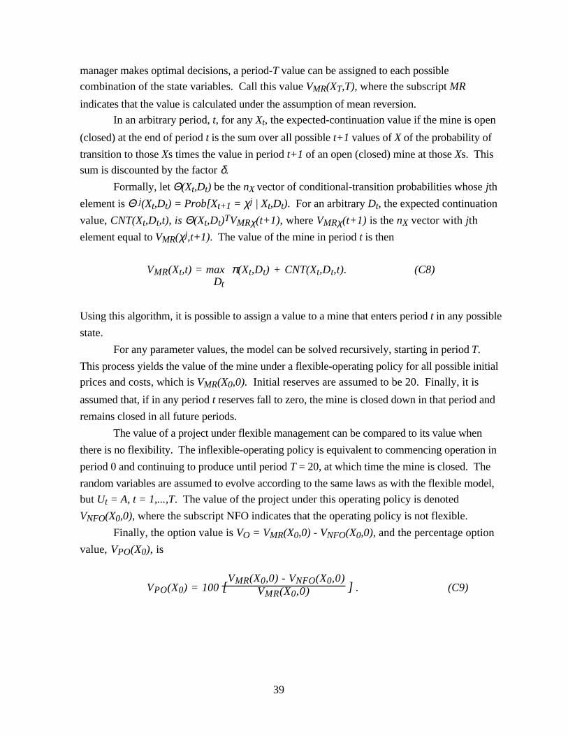
39

manager makes optimal decisions, a period-T value can be assigned to each possible

combination of the state variables. Call this value VMR(XT,T), where the subscript MR

indicates that the value is calculated under the assumption of mean reversion.

In an arbitrary period, t, for any Xt, the expected-continuation value if the mine is open

(closed) at the end of period t is the sum over all possible t+1 values of X of the probability of

transition to those Xs times the value in period t+1 of an open (closed) mine at those Xs. This

sum is discounted by the factor δ.

Formally, let Θ(Xt,Dt) be the nX vector of conditional-transition probabilities whose jth

element is Θ j(Xt,Dt) = Prob[Xt+1 = χj | Xt,Dt). For an arbitrary Dt, the expected continuation

value, CNT(Xt,Dt,t), is Θ(Xt,Dt)TVMRχ(t+1), where VMRχ(t+1) is the nX vector with jth

element equal to VMR(χj,t+1). The value of the mine in period t is then

VMR(Xt,t) = max π(Xt,Dt) + CNT(Xt,Dt,t). (C8)Dt

Using this algorithm, it is possible to assign a value to a mine that enters period t in any possible

state.

For any parameter values, the model can be solved recursively, starting in period T.

This process yields the value of the mine under a flexible-operating policy for all possible initial

prices and costs, which is VMR(X0,0). Initial reserves are assumed to be 20. Finally, it is

assumed that, if in any period t reserves fall to zero, the mine is closed down in that period and

remains closed in all future periods.

The value of a project under flexible management can be compared to its value when

there is no flexibility. The inflexible-operating policy is equivalent to commencing operation in

period 0 and continuing to produce until period T = 20, at which time the mine is closed. The

random variables are assumed to evolve according to the same laws as with the flexible model,

but Ut = A, t = 1,...,T. The value of the project under this operating policy is denoted

VNFO(X0,0), where the subscript NFO indicates that the operating policy is not flexible.

Finally, the option value is VO = VMR(X0,0) - VNFO(X0,0), and the percentage option

value, VPO(X0), is

VPO(X0) = 100 [VMR(X0,0) - VNFO(X0,0)

VMR(X0,0) ] . (C9)

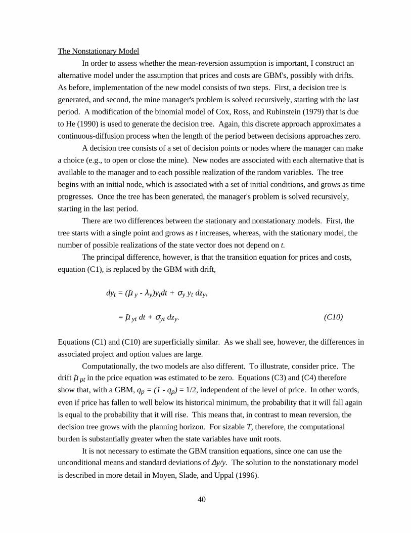
40

The Nonstationary Model

In order to assess whether the mean-reversion assumption is important, I construct an

alternative model under the assumption that prices and costs are GBM's, possibly with drifts.

As before, implementation of the new model consists of two steps. First, a decision tree is

generated, and second, the mine manager's problem is solved recursively, starting with the last

period. A modification of the binomial model of Cox, Ross, and Rubinstein (1979) that is due

to He (1990) is used to generate the decision tree. Again, this discrete approach approximates a

continuous-diffusion process when the length of the period between decisions approaches zero.

A decision tree consists of a set of decision points or nodes where the manager can make

a choice (e.g., to open or close the mine). New nodes are associated with each alternative that is

available to the manager and to each possible realization of the random variables. The tree

begins with an initial node, which is associated with a set of initial conditions, and grows as time

progresses. Once the tree has been generated, the manager's problem is solved recursively,

starting in the last period.

There are two differences between the stationary and nonstationary models. First, the

tree starts with a single point and grows as t increases, whereas, with the stationary model, the

number of possible realizations of the state vector does not depend on t.

The principal difference, however, is that the transition equation for prices and costs,

equation (C1), is replaced by the GBM with drift,

dyt = (µ y - λy)ytdt + σy yt dzy,

= µ yt dt + σyt dzy. (C10)

Equations (C1) and (C10) are superficially similar. As we shall see, however, the differences in

associated project and option values are large.

Computationally, the two models are also different. To illustrate, consider price. The

drift µ pt in the price equation was estimated to be zero. Equations (C3) and (C4) therefore

show that, with a GBM, qp = (1 - qp) = 1/2, independent of the level of price. In other words,

even if price has fallen to well below its historical minimum, the probability that it will fall again

is equal to the probability that it will rise. This means that, in contrast to mean reversion, the

decision tree grows with the planning horizon. For sizable T, therefore, the computational

burden is substantially greater when the state variables have unit roots.

It is not necessary to estimate the GBM transition equations, since one can use the

unconditional means and standard deviations of ∆y/y. The solution to the nonstationary model

is described in more detail in Moyen, Slade, and Uppal (1996).

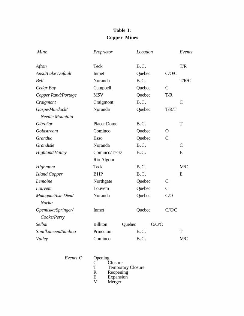
Table I:

Copper Mines

Mine Proprietor Location Events

Afton Teck B.C. T/R

Ansil/Lake Dufault Inmet Quebec C/O/C

Bell Noranda B.C. T/R/C

Cedar Bay Campbell Quebec C

Copper Rand/Portage MSV Quebec T/R

Craigmont Craigmont B.C. C

Gaspe/Murdock/ Noranda Quebec T/R/T

Needle Mountain

Gibraltar Placer Dome B.C. T

Goldstream Cominco Quebec O

Granduc Esso Quebec C

Grandisle Noranda B.C. C

Highland Valley Cominco/Teck/ B.C. E

Rio Algom

Highmont Teck B.C. M/C

Island Copper BHP B.C. E

Lemoine Northgate Quebec C

Louvem Louvem Quebec C

Matagami/Isle Dieu/ Noranda Quebec C/O

Norita

Opemiska/Springer/ Inmet Quebec C/C/C

Cooke/Perry

Selbai Billiton Quebec O/O/C

Similkameen/Simlico Princeton B.C. T

Valley Cominco B.C. M/C

Events:O OpeningC ClosureT Temporary ClosureR ReopeningE ExpansionM Merger

Table II:

Summary Statistics

IIa: Yearly Data

Variable # of

Obs.

Mean Standard

Deviation

Minimum Maximum Units

PRICE 14a 142.3 33.4 110.1 223.9 ¢/lbc

∆P/P 13a -0.039 0.169 -0.274 0.326 unit free

PRICE 75b 138.6 33.3 82.7 237.2 ¢/lbc

∆P/P 75b 0.004 0.136 -0.329 0.326 unit free

COST 175 108.0 29.9 46.8 205.6 ¢/lbc

∆C/C 152 0.029 0.253 -0.424 1.388 unit free

RESERVES 168 100.5 180.3 0.074 852.8 106 tonnes

∆R/R 140 0.013 1.19 -0.813 12.67 unit free

ORE 185 6.52 9.68 0.032 46.3 106 tonnes/yr

∆O/O 160 0.068 0.645 -0.893 6.50 unit free

METAL 184 26.7 33.1 0.015 177.4 103 tonnes/yr

∆Q/Q 158 0.140 1.12 -0.947 9.212 unit free

GRADE 187 1.15 1.26 0.150 8.200 percent

∆G/G 162 0.079 0.792 -0.615 8.377 unit free

CU 185 76.9 28.5 5.52 156.6 percent

∆CU/CU 160 0.065 0.649 -0.856 6.50 unit free

a) 1980-1993, b) 1918-1993, All other data from a panel of 21 mines between 1980-1993c) Real Canadian (1993) cents per pound

IIb: Monthly Data, 1980-1993

Variable # of

Obs.

Mean Standard

Deviation

Minimum Maximum Units

PRICE 168 142.8 35.5 96.6 310.4 ¢/lba

∆P/P 167 -0.004 0.063 -0.207 0.287 unit free

a) Real Canadian (1993) cents per pound

Table V:

Other Model Parameters

Model Parameters

Variable Name Value Units

Time between decisions ∆t 0.25 Years

Planning horizon T 20.0 Years

Risk-free rate of interest r 5.0 Percent

Opening cost Co 10.0 CAN ¢/lb

Closing cost Cc 20.0 CAN ¢/lb

Maintenance cost Cm 2.0 CAN ¢/lb/yr

Profit-tax rate τ 25.0 Percent

Mean price p 135.0 CAN ¢/lb

Price drift parameter, GBMa µ p 0.0 Unit free

Price risk premiumc λp 0.0 Percent

Cost drift parameter, GBMb µ c 0.0 Unit free

Cost risk premiumb λc 0.0 Percent

Reserve risk premiumb λR 0.0 Percent

a) From an equation of the form ∆y/y = µ∆t + σ∆z.b) From a capital-asset-pricing model.

Table VI:

Comparison of Flexible and NUN Project Values

Mine Initially OpenNUN = No Uncertainty

MR = Flexible Policy with Mean-Reverting Prices and CostsGBM = Flexible Policy with GBM Prices and Costs

NUN Discount Rate = 5% per year

C0 = C

CAN ¢/lb

VNUN VM R VGBM

Difference

and

% Differencea

MR

Difference

and

% Differenceb

GBM

98 346.4 357.0 502.3 (10.6) [3.0] (155.9) [31.0]

108 250.8 274.5 445.0 (23.7) [8.6] (194.2) [43.6]

120 136.0 188.3 383.9 (52.3) [27.8] (247.9) [64.6]

NUN Discount Rate = 15% per year

C0 = C

CAN ¢/lb

VNUN VM R VGBM

Difference

and

% Differencea

MR

Difference

and

% Differenceb

GBM

98 180.8 357.0 502.3 (176.2) [49.4] (321.5) [64.0]

108 131.6 274.5 445.0 (142.9) [52.1] (313.4) [70.4]

120 72.6 188.3 383.9 (115.7) [61.4] (311.3) [81.1]

Average price: 135¢/lb, Risk-free rate: 5%/yr, Profit-tax rate: 25%,Reopening cost: 10¢/lb, Closing cost: 20¢/lb, Maintenance cost: 2¢/lb/yr

Costs and prices in real (1993) Canadian ¢/lb

a) (VMR - VNUN) and [100(VMR - VNUN)/VMR]

b) (VGBM - VNUN) and [100(VGBM - VNUN)/VGBM]

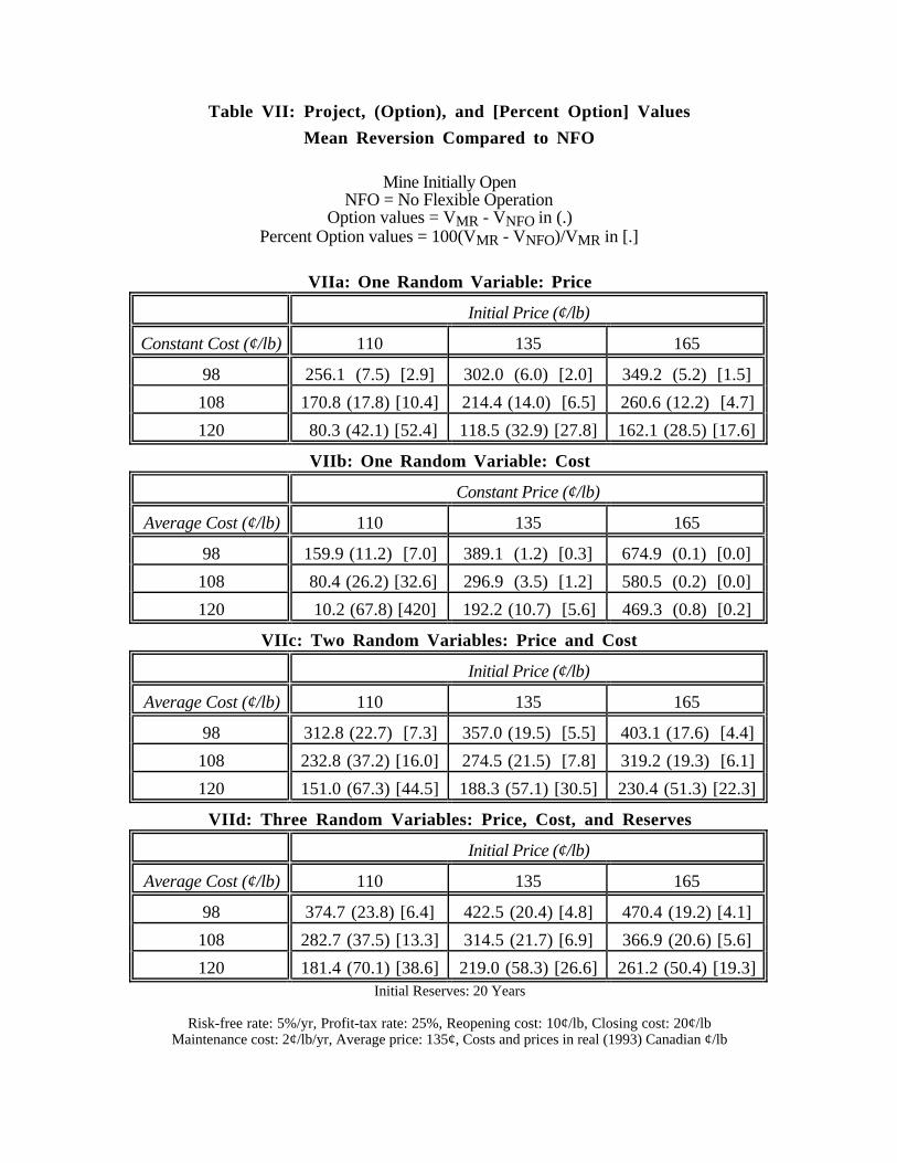
Table VII: Project, (Option), and [Percent Option] Values

Mean Reversion Compared to NFO

Mine Initially OpenNFO = No Flexible Operation

Option values = VMR - VNFO in (.)Percent Option values = 100(VMR - VNFO)/VMR in [.]

VIIa: One Random Variable: Price

Initial Price (¢/lb)

Constant Cost (¢/lb) 110 135 165

98 256.1 (7.5) [2.9] 302.0 (6.0) [2.0] 349.2 (5.2) [1.5]

108 170.8 (17.8) [10.4] 214.4 (14.0) [6.5] 260.6 (12.2) [4.7]

120 80.3 (42.1) [52.4] 118.5 (32.9) [27.8] 162.1 (28.5) [17.6]

VIIb: One Random Variable: Cost

Constant Price (¢/lb)

Average Cost (¢/lb) 110 135 165

98 159.9 (11.2) [7.0] 389.1 (1.2) [0.3] 674.9 (0.1) [0.0]

108 80.4 (26.2) [32.6] 296.9 (3.5) [1.2] 580.5 (0.2) [0.0]

120 10.2 (67.8) [420] 192.2 (10.7) [5.6] 469.3 (0.8) [0.2]

VIIc: Two Random Variables: Price and Cost

Initial Price (¢/lb)

Average Cost (¢/lb) 110 135 165

98 312.8 (22.7) [7.3] 357.0 (19.5) [5.5] 403.1 (17.6) [4.4]

108 232.8 (37.2) [16.0] 274.5 (21.5) [7.8] 319.2 (19.3) [6.1]

120 151.0 (67.3) [44.5] 188.3 (57.1) [30.5] 230.4 (51.3) [22.3]

VIId: Three Random Variables: Price, Cost, and Reserves

Initial Price (¢/lb)

Average Cost (¢/lb) 110 135 165

98 374.7 (23.8) [6.4] 422.5 (20.4) [4.8] 470.4 (19.2) [4.1]

108 282.7 (37.5) [13.3] 314.5 (21.7) [6.9] 366.9 (20.6) [5.6]

120 181.4 (70.1) [38.6] 219.0 (58.3) [26.6] 261.2 (50.4) [19.3]Initial Reserves: 20 Years

Risk-free rate: 5%/yr, Profit-tax rate: 25%, Reopening cost: 10¢/lb, Closing cost: 20¢/lbMaintenance cost: 2¢/lb/yr, Average price: 135¢, Costs and prices in real (1993) Canadian ¢/lb

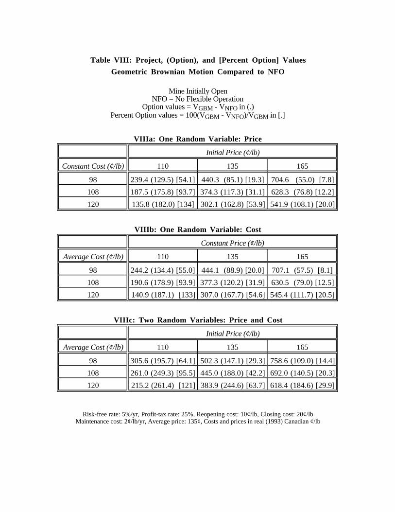
Table VIII: Project, (Option), and [Percent Option] Values

Geometric Brownian Motion Compared to NFO

Mine Initially OpenNFO = No Flexible Operation

Option values = VGBM - VNFO in (.)Percent Option values = 100(VGBM - VNFO)/VGBM in [.]

VIIIa: One Random Variable: Price

Initial Price (¢/lb)

Constant Cost (¢/lb) 110 135 165

98 239.4 (129.5) [54.1] 440.3 (85.1) [19.3] 704.6 (55.0) [7.8]

108 187.5 (175.8) [93.7] 374.3 (117.3) [31.1] 628.3 (76.8) [12.2]

120 135.8 (182.0) [134] 302.1 (162.8) [53.9] 541.9 (108.1) [20.0]

VIIIb: One Random Variable: Cost

Constant Price (¢/lb)

Average Cost (¢/lb) 110 135 165

98 244.2 (134.4) [55.0] 444.1 (88.9) [20.0] 707.1 (57.5) [8.1]

108 190.6 (178.9) [93.9] 377.3 (120.2) [31.9] 630.5 (79.0) [12.5]

120 140.9 (187.1) [133] 307.0 (167.7) [54.6] 545.4 (111.7) [20.5]

VIIIc: Two Random Variables: Price and Cost

Initial Price (¢/lb)

Average Cost (¢/lb) 110 135 165

98 305.6 (195.7) [64.1] 502.3 (147.1) [29.3] 758.6 (109.0) [14.4]

108 261.0 (249.3) [95.5] 445.0 (188.0) [42.2] 692.0 (140.5) [20.3]

120 215.2 (261.4) [121] 383.9 (244.6) [63.7] 618.4 (184.6) [29.9]

Risk-free rate: 5%/yr, Profit-tax rate: 25%, Reopening cost: 10¢/lb, Closing cost: 20¢/lbMaintenance cost: 2¢/lb/yr, Average price: 135¢, Costs and prices in real (1993) Canadian ¢/lb

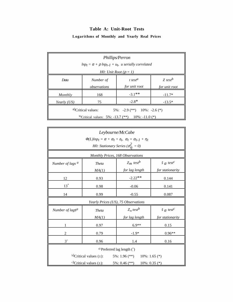
Table A: Unit-Root Tests

Logarithms of Monthly and Yearly Real Prices

Phillips/Perron

lnpt = α + ρ lnpt-1 + ut, u serially correlated

H0: Unit Root (ρ = 1)

Data Number of

observations

t testa

for unit root

Z testb

for unit root

Monthly 168 -3.1** -11.7*

Yearly (US) 75 -2.8* -13.5*

a)Critical values: 5%: -2.9 (**) 10%: -2.6 (*)

b)Critical values: 5%: -13.7 (**) 10%: -11.0 (*)

Leybourne/McCabe

Φ(L)lnpt = α + αt + εt, αt = αt-1 + ηt

H0: Stationary Series (σ2η = 0)

Monthly Prices, 168 Observations

Number of lags a Theta

MA(1)

Zm testb

for lag length

s α testc

for stationarity

12 0.93 -2.22** 0.144

13 0.98 -0.06 0.141

14 0.99 -0.55 0.087

Yearly Prices (US), 75 Observations

Number of lagsa Theta

MA(1)

Zm testb

for lag length

s α testc

for stationarity

1 0.97 6.9** 0.15

2 0.79 -1.9* 0.96**

3˚ 0.96 1.4 0.16

a) Preferred lag length (˚)

b)Critical values (±): 5%: 1.96 (**) 10%: 1.65 (*)

c)Critical values (±): 5%: 0.46 (**) 10%: 0.35 (*)

Table III:

Transition Equations

IIIa: Yearly Prices and Costs

xt - xt -1xt-1

= [α + β1xt-1 + β2xt-2 + γTyt]∆t + σ ∆Z

Dependent

Variable

# of

Obs.

Constant x-1 x-2 %∆METAL

Sum

lagged

variables

P value

lagged

variables

P value

EOS

σ R2

PRICEa) 13 -0.039

(-0.8)

0.169

PRICEa)

*

13 0.377

(2.0)

-0.0029

(-2.3)

-0.003 0.02 0.139 0.33

PRICEa) 12 0.458

(1.9)

-0.0005

(-0.2)

-0.0028

(-1.9)

-0.003 0.04 0.123 0.42

COSTb) 137 -0.415

(-2.8)

0.00 0.230 0.24

COSTb)

*

137 -0.0029

(-4.2)

-0.433

(-4.2)

-0.003 0.00 0.00 0.222 0.29

COSTb) 125 -0.0021

(-2.3)

-0.0007

(-0.7)

-0.500

(-4.9)

-0.003 0.00 0.00 0.216 0.26

t statistics in parenthesesa) OLS estimates

b) IV estimates, Mine fixed effects not shown* indicates an equation that is used in the numerical solutions

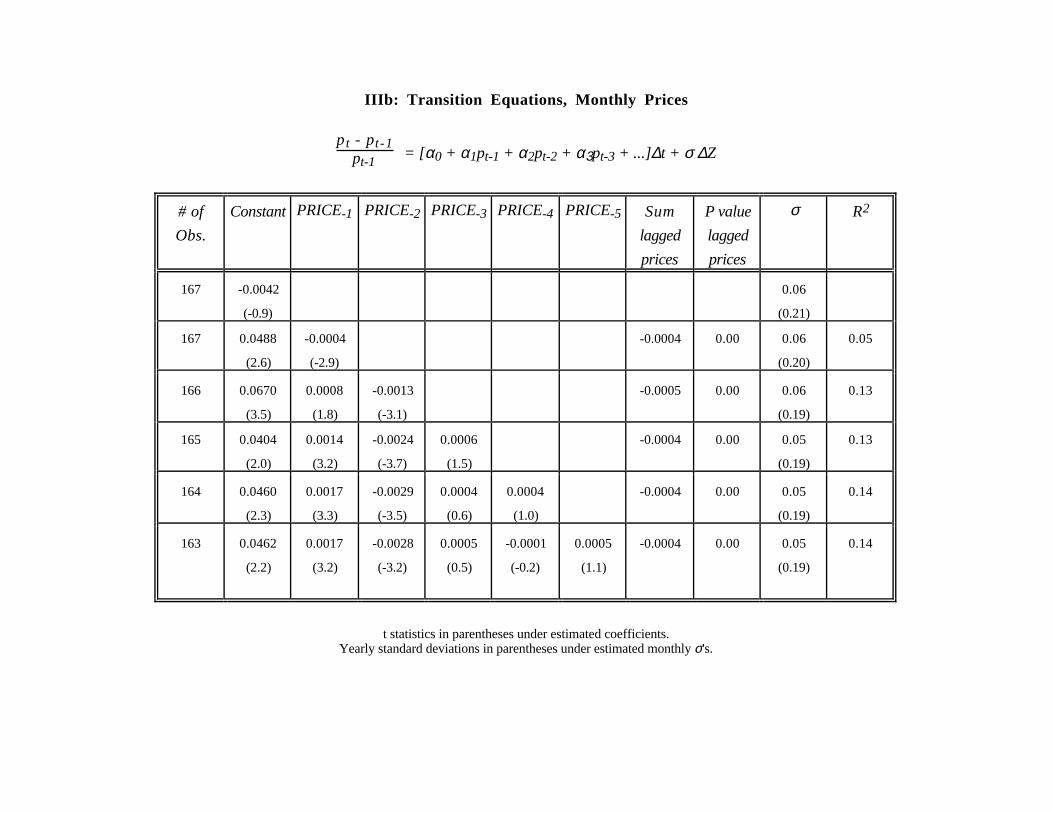
IIIb: Transition Equations, Monthly Prices

pt - pt-1pt-1

= [α0 + α1pt-1 + α2pt-2 + α3pt-3 + ...]∆t + σ ∆Z

# of

Obs.

Constant PRICE-1 PRICE-2 PRICE-3 PRICE-4 PRICE-5 Sum

lagged

prices

P value

lagged

prices

σ R2

167 -0.0042

(-0.9)

0.06

(0.21)

167 0.0488

(2.6)

-0.0004

(-2.9)

-0.0004 0.00 0.06

(0.20)

0.05

166 0.0670

(3.5)

0.0008

(1.8)

-0.0013

(-3.1)

-0.0005 0.00 0.06

(0.19)

0.13

165 0.0404

(2.0)

0.0014

(3.2)

-0.0024

(-3.7)

0.0006

(1.5)

-0.0004 0.00 0.05

(0.19)

0.13

164 0.0460

(2.3)

0.0017

(3.3)

-0.0029

(-3.5)

0.0004

(0.6)

0.0004

(1.0)

-0.0004 0.00 0.05

(0.19)

0.14

163 0.0462

(2.2)

0.0017

(3.2)

-0.0028

(-3.2)

0.0005

(0.5)

-0.0001

(-0.2)

0.0005

(1.1)

-0.0004 0.00 0.05

(0.19)

0.14

t statistics in parentheses under estimated coefficients.Yearly standard deviations in parentheses under estimated monthly σ's.

III c: Transition Equations, Yearly Reserves Net of Extraction

∆Nt = Rt - Rt-1 + Ot-1

Kt-1 = [ α0 + α1Nt-1 + α2Nt-2 + α3Nt-3 + β1pt-1 + β2pt-2 + γ1ct-1 + γ2ct-2]∆t + σ∆Z

Number

of Obs.

p-1 p-2 c-1 c-2 N-1 N-2 N-3 P value

Σp-i

P value

Σc-i

P value

ΣN-i

P value

Joint

σ R2

115

*

1.56 0.26

115 0.001

(0.5)

0.65 1.56 0.26

107 -0.004

(-1.0)

0.30 1.61 0.27

115 -0.005

(-1.8)

0.07 1.54 0.26

99 0.008

(1.2)

-0.009

(-1.2)

0.48 1.57 0.30

95 -0.014

(-1.4)

0.012

(1.1)

0.36 1.90 0.26

93 -0.022

(-2.8)

0.017

(2.2)

0.01 1.47 0.41

73 -0.009

(-1.1)

-0.009

(-0.8)

0.013

(1.7)

0.13 1.37 0.25

87 0.012

(1.4)

-0.007

(-0.9)

-0.012

(-1.1)

0.004

(0.4)

-0.023

(-2.7)

0.018

(2.1)

0.37 0.53 0.01 0.08 1.48 0.44

t statistics in parentheses, Mine fixed effects not shown* indicates an equation that is used in the numerical solutions

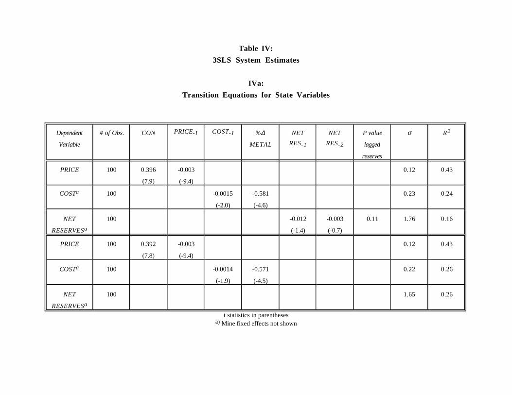
Table IV:

3SLS System Estimates

IVa:

Transition Equations for State Variables

Dependent

Variable

# of Obs. CON PRICE-1 COST-1 %∆

METAL

NET

RES-1

NET

RES-2

P value

lagged

reserves

σ R2

PRICE 100 0.396

(7.9)

-0.003

(-9.4)

0.12 0.43

COSTa 100 -0.0015

(-2.0)

-0.581

(-4.6)

0.23 0.24

NET

RESERVESa

100 -0.012

(-1.4)

-0.003

(-0.7)

0.11 1.76 0.16

PRICE 100 0.392

(7.8)

-0.003

(-9.4)

0.12 0.43

COSTa 100 -0.0014

(-1.9)

-0.571

(-4.5)

0.22 0.26

NET

RESERVESa

100 1.65 0.26

t statistics in parenthesesa) Mine fixed effects not shown

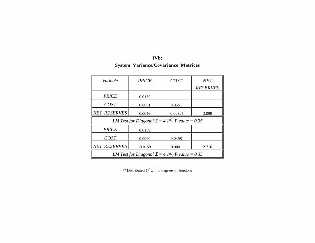
IVb:

System Variance/Covariance Matrices

Variable PRICE COST NET

RESERVES

PRICE 0.0139

COST 0.0061 0.0561

NET RESERVES 0.0046 -0.00395 3.099

LM Test for Diagonal Σ = 4.1a), P value = 0.35

PRICE 0.0139

COST 0.0060 0.0498

NET RESERVES -0.0159 0.0001 2.716

LM Test for Diagonal Σ = 4.1a), P value = 0.35

a) Distributed χ2 with 3 degrees of freedom

Table B:

Unit-Cost Functions

ct = β'xt + ut

# of Obs. GRADE GRADEx

DOPEN

GRADEx

DUNDER

RES/CAP CU WAGE ENERGY

PRICE

INDPROD σ R2

155 -4.451

(-3.2)

-0.387

(-1.5)

-51.36

(-2.5)

-3.567

(-0.2)

31.38

(4.7)

71.99

(6.7)

23.9 0.39

155 -160.3

(-6.2)

-0.310

(-1.4)

-13.63

(-0.7)

9.44

(0.6)

23.38

(4.0)

54.65

(6.1)

20.8 0.54

155 0.259

(0.1)

-0.399

(-1.6)

-46.35

(-2.3)

-1.867

(-0.1)

30.55

(4.6)

66.80

(4.6)

23.9 0.39

Instrumental varaibles estimatest statistics in parentheses

Mine fixed effects not shown

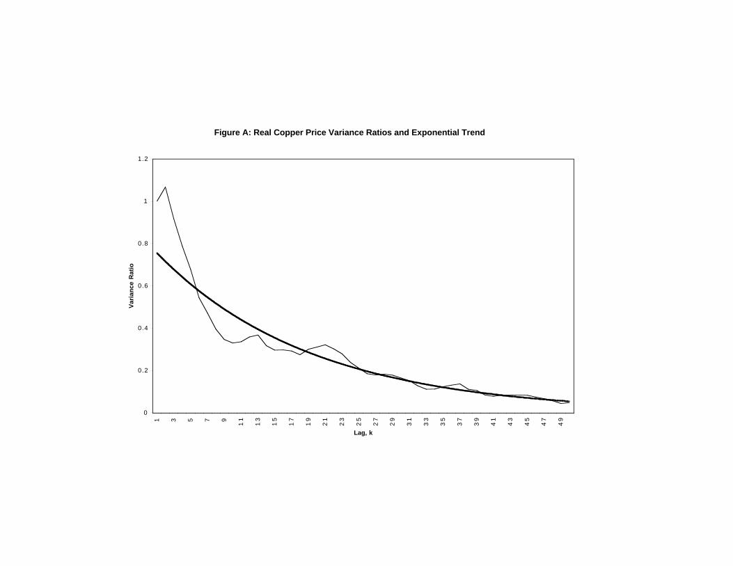
Figure A: Real Copper Price Variance Ratios and Exponential Trend

0

0.2

0.4

0.6

0.8

1

1.21 3 5 7 9

11

13

15

17

19

21

23

25

27

29

31

33

35

37

39

41

43

45

47

49

Lag, k

Var

ianc

e R

atio