Value Regularization and Fenchel Dualityjmlr.csail.mit.edu/papers/volume8/rifkin07a/rifkin07a.pdf · the combination of value regularization and Fenchel duality are valuable tools

Journal of Machine Learning Research 8 (2007) 441-479 Submitted 3/06; Revised 10/06; Published 3/07

Value Regularization and Fenchel Duality

Ryan M. Rifkin [email protected]

Honda Research Institute USA, Inc.One Cambridge Center, Suite 401Cambridge, MA 02142, USA

Ross A. Lippert [email protected]

Department of MathematicsMassachusetts Institute of Technology77 Massachusetts AvenueCambridge, MA 02139-4307, USA

Editor: Peter Bartlett

AbstractRegularization is an approach to function learning that balances fit and smoothness. In practice,we search for a function f with a finite representation f = ∑i ciφi(·). In most treatments, the ci

are the primary objects of study. We consider value regularization, constructing optimization prob-lems in which the predicted values at the training points are the primary variables, and thereforethe central objects of study. Although this is a simple change, it has profound consequences. Fromconvex conjugacy and the theory of Fenchel duality, we derive separate optimality conditions forthe regularization and loss portions of the learning problem; this technique yields clean and shortderivations of standard algorithms. This framework is ideally suited to studying many other phe-nomena at the intersection of learning theory and optimization. We obtain a value-based variantof the representer theorem, which underscores the transductive nature of regularization in repro-ducing kernel Hilbert spaces. We unify and extend previous results on learning kernel functions,with very simple proofs. We analyze the use of unregularized bias terms in optimization problems,and low-rank approximations to kernel matrices, obtaining new results in these areas. In summary,the combination of value regularization and Fenchel duality are valuable tools for studying theoptimization problems in machine learning.Keywords: kernel machines, duality, optimization, convex analysis, kernel learning

1. Introduction

Given a set of training data (X1,Y1), . . . ,(Xn,Yn), the inductive supervised learning task is to learna function f that, given a new X value, will predict the associated Y value. A common frameworkfor solving this problem is Tikhonov regularization (Tikhonov and Arsenin, 1977):

inff∈F

n

∑i=1

v( f (Xi),Yi)+λ2

Ω( f )

. (1)

In this general form, F is a space of functions from which f must be selected, and v( f (Xi),Yi)is the loss, indicating the penalty we pay when we see Xi, predict f (Xi), and the true value is Yi. Fora large class of functions F , simply minimizing ∑n

i=1 v( f (Xi),Yi) directly is ill-posed and leads tooverfitting the training data. We restore well-posedness by introducing a regularization term Ω( f )

c©2007 Ryan M. Rifkin and Ross A. Lippert.

RIFKIN AND LIPPERT

that penalizes elements of f that are too “complex”. The regularization parameter, λ, controls thetradeoff between finding a function of low complexity and fitting the training data.

A large amount of work (Wahba, 1990; Evgeniou et al., 2000) takes F to be a reproducingkernel Hilbert space (RKHS) H (Aronszajn, 1950) induced by a kernel function k. In this situation,we rewrite (1) as

inff∈H

n

∑i=1

v( f (Xi),Yi)+λ2|| f ||2k

, (2)

indicating that the regularization term is now the squared norm of the function in the RKHS.Many common algorithms, including support vector machines for classification (Cortes and Vapnik,1995) and regression (Vapnik, 1998), regularized least squares (Wahba, 1990; Poggio and Girosi,1990; Rifkin, 2002), and kernel logistic regression (Jaakkola and Haussler, 1999) are instances ofTikhonov regularization: different loss functions yield different algorithms.1

A consequence of the so-called representer theorem (Wahba, 1990; Scholkopf et al., 2001), isthat the minimizer of (2) will have the form

f (x) =n

∑i=1

cik(x,Xi). (3)

In other words, in an RKHS, a function f which minimizes (2) is a sum of kernel functions k(·,Xi)over the data points. We solve a Tikhonov regularization (or, equivalently, train a predictor) byfinding the coefficients ci. Assuming that the loss function is convex, the minimization of (2) (or(1)) is tractable.

Defining K as the n × n kernel matrix with Ki j = k(Xi,X j), the regularization penalty || f ||2kbecomes ctKc, the output at training point i is given by f (Xi) = ∑n

j=1 c jk(Xi,X j) = (Kc)i, and wecan rewrite (2) as

infc∈Rn

n

∑i=1

v((Kc)i,Yi)+λ2

ctKc

. (4)

Regularizing in an RKHS is special in that it has a representer theorem: the optimal solutionin an infinite-dimensional space of functions is found by solving a finite dimensional minimizationproblem. Although most other function space regularizers do not have similar properties, we mayconsider other regularizers as modifications of (4): replacing ctKc with ctc, we obtain ridge re-gression (Tikhonov and Arsenin, 1977), and replacing it with ∑n

i=1 |ci|, we obtain L1-regularization(Zhu et al., 2003). In such cases, we are assuming that we are looking for a function of the form(3) a priori. There is nothing wrong with this, but it should not be confused with the case of RKHSregularization, where (3) arises naturally from a search for an optimizing function.

In general, an equation like (4) is used as the starting point for thinking algorithmically aboutfinding c. For example, in a standard development of support vector machines (Cristianini andShaw-Taylor, 2000; Rifkin, 2002), one starts with (4) instantiated with the SVM hinge lossv( f (Xi),Yi) = (1−yi f (Xi))+, introducing slack variables ξi = v( f (Xi),Yi) and constraints to handle

1. Technically speaking, to derive an algorithm such as the classic SVM one also needs an unregularized bias term b:this issue is discussed in detail later in the paper.

442

VALUE REGULARIZATION AND FENCHEL DUALITY

the non-differentiability of the hinge loss at 0 as well as an unregularized bias term b, yielding aquadratic program:2

minc∈Rn,ξ∈Rn,b∈R

1n ∑n

i=1 ξi +λcT Kc

subject to : Yi(

∑nj=1 c jk(Xi,X j)+b

)

≥ 1−ξi i = 1, . . . ,n

ξi ≥ 0 i = 1, . . . ,n.

This program is called the primal problem. In order to expose sparsity in the solution, the La-grangian dual is taken, yielding the dual problem:

maxα∈Rn

∑ni=1 αi − 1

(2λ)2 αtdiag(Y )Kdiag(Y )α

subject to : ∑ni=1Yiαi = 0

0 ≤ αi ≤ 1n i = 1, . . . ,n.

It is then observed that the dual problem is easier to solve (because of its simpler constraint struc-ture), and that solutions to the primal can be easily obtained from solutions to the dual.

We propose to take a different approach to Tikhonov regularization, that we believe to be morefundamental. The approach rests on two ideas.

First, we consider the predicted values yi ≡ f (Xi) = (Kc)i to be the central objects of study, andwrite our optimization problems in terms of y. In the case of RKHS regularization with a positive-definite kernel, the matrix K is typically non-singular (Micchelli, 1986), 3 and we rewrite (4) as avalue regularization:

infy∈Rn

λ2

ytK−1y+n

∑i=1

v(yi,Yi)

.

Although this is a simple transformation, the consequences are far-reaching. Looking at the rewrit-ten problem, we notice that the kernel matrix K appears only in the regularization—it does notappear in the loss term. This is intuitive, as the loss function (of course) cares only about thepredicted outputs, not what combination of kernel coefficients generated those predicted outputs.Additionally, we see that the loss function decomposes into n separate single-point loss functions.In contrast, if the ci are the primary variables, the loss at each data point is a function of the entire cvector.

The benefits of value regularization are greatly amplified by the second central idea of this work:instead of Lagrangian duality, we use Fenchel duality (Borwein and Lewis, 2000), a form of dualitythat is well-matched to the problems of learning theory. Although we discuss Fenchel duality ingreater detail below, we present a brief overview here. Consider an optimization problem of theform:

infy∈Rn

f (y)+g(y). (5)

2. Traditional derivations parametrize the loss function instead of the regularization, with a constant C = 12λ , but that is

a minor point.3. Throughout this paper, when we work with an RKHS regularizer we will generally assume that the kernel function is

positive definite and the points are in general position, implying the existence of K−1. This assumption can be easilyrelaxed using pseudoinverses, although the mathematics becomes somewhat more cumbersome.

443

RIFKIN AND LIPPERT

Fenchel duality defines a so-called Fenchel dual:

supz∈Rn

− f ∗(z)−g∗(−z), (6)

where f ∗,g∗ are Fenchel-Legendre conjugates (definition 4) computed via auxiliary (and by design,simpler) optimization problems on f and g separately. Convexity of f and g (and some topologicalqualifications) ensure that the optimal objective values of (5) and (6) are equivalent, and that anyoptimal y and z satisfy:

f (y)− ytz+ f ∗(z) = 0

g(y)+ ytz+g∗(−z) = 0.

Fenchel duality encompasses other notions of duality such as Lagrangian duality and seems tobe a natural concept to apply to regularization problems where f and g each arise from differentconsiderations—for supervised learning problems, one will come from regularization and the otherfrom empirical loss.

Elaborating on this idea, Fenchel duality gives us a separation of concerns which is not presentin the Lagrangian approach. The point of formulating an optimization problem such as a quadraticprogram is ultimately to derive optimality conditions and algorithms for finding optimal solutions.For convex optimization problems, all local optima are globally optimal, and we can formulatea complete set of optimality conditions which the primal and dual solutions will simultaneouslysatisfy. These are generally known as the Karush-Kuhn-Tucker (KKT) conditions (Bazaraa et al.,1993).4 Fenchel duality makes it clear that the two functions f and g, or, in our case, the loss termand the regularization, contribute individual local optimality conditions, and the total optimalityconditions for the overall problem are simply the union of the individual optimality conditions.Put differently, using Fenchel duality, we can derive a table for nr regularizations and nl losses,and immediately combine these to derive optimality conditions for nrnl learning problems. Thisidea is obscured by the Lagrangian duality approach to deriving optimality conditions for learningproblems. As an example, for the common case of the RKHS regularizer 1

2 ytK−1y, we will find thatthe primal-dual relationship is given by y = λ−1Kz. This condition is independent of the loss—itshows up simultaneously in SVM, regularized least squares, and logistic regression.

Value regularization and Fenchel duality reinforce each other’s strengths. Because the kernelaffects only the regularization term and not the loss term, applying Fenchel duality to value regular-ization yields extremely clean formulations. The major contribution of this paper is the combinationof value regularization and Fenchel duality in a framework that yields new insights into many of theoptimization problems that arise in learning theory.

We present, in Section 3, a primer on convex analysis and Fenchel duality, with emphasis onthe key ideas that are needed for learning theory. We believe that this section provides a sufficientlyself-contained summary of convex analysis to allow a machine learning researcher to apply ourframework to new problems.

In Section 4, we specialize the convex analysis results to Tikhonov value regularizations con-sisting of the sum of a regularization and a loss term. Section 5 specializes the result further to theRKHS case and obtains very simple derivations of well-known kernel machines.

Section 6 is concerned with value regularization in the context of L1 regularization, a regular-ization with the explicit goal of obtaining sparsity in the finite representation. In Section 6.1, we

4. The complete KKT conditions for SVM can be found (among other places) in Rifkin (2002).

444


briefly discuss 1-norm support vector machines, and emphasize a key distinction between RKHSand other regularizations: in RKHS regularization, the ci, which are the expansion coefficients inthe finite representation of the learned function, and the zi, which are the dual variables associatedwith the yi in the value regularization problem, are identifiable (z = λ−1c). This is a consequenceof the RKHS regularization, and does not hold for more general regularizations. In Section 6.2, wepresent a simpler derivation of the relationship between support vector regression and sparse ap-proximation, first discovered in Girosi (1998); essentially, the problems are duals, with the width ofthe ε-tube in the support vector regression problem becoming the sparsity regularizer in the sparseapproximation problem.

In Section 7, we develop a new view of the representer theorem, in the context of value regular-ization. The common wisdom about the representer theorem is that it guarantees that the solutionto an optimization problem in an (infinite-dimensional) function space has a finite representation asan expansion of kernel functions around the training points. While this is certainly true, we gainadditional insights by considering an augmented problem in which the test points also appear inthe regularization, but not in the loss. In the augmented optimization problem the predicted out-puts at the training points do not change, and the expansion coefficients at the test points vanish—arepresenter theorem. This underscores the fact that for supervised learning in an RKHS, inductionand transduction are identical. In the context of transductive or semi-supervised algorithms, thepicture is more complex. There have been several recent articles that turn transductive algorithmsinto semi-supervised algorithms via an appeal to the representer theorem. While this is formallyvalid, the resulting transductive algorithm is not equivalent to the semi-supervised algorithm, andthe transductive algorithm is perhaps the more “natural” choice. Section 7.1 is devoted to a discus-sion of this topic.

Recently, there has been interest in “learning the kernel”. In Section 8, we may view this as avalue regularization where the kernel matrix itself is an auxiliary parameter to be optimized. Thevalue-based formulation is ideal here, because the kernel appears only in the regularization term andnot in the loss term. We first derive a general result that gives optimality conditions for a generalconvex penalty F(K) on the kernel matrix. Work to date has considered only the case where F is0 for some set of semi-definite matrices, and infinite otherwise. Lanckriet et al. (2004) considers acase where the kernel function is a linear combination of a finite set of kernels; we will see that aminor modification to their formulation yields a representer theorem and an agreement of inductiveand transductive algorithms. Argyriou et al. (2005) work with a convex set generated by an infinite,continuously parametrized set of kernel functions. We give proofs of their main results which areshorter and simpler, and also more general, allowing arbitrary convex loss functions (Argyriou et al.(2005) requires differentiability).

In Section 9, we show how infimal convolutions, a form of optimization relaxation (see Section3.4) are useful in learning theory. We first explore the idea of “biased” regularizations, the best-known example being the unregularized bias term b in the standard formulation of support vectormachines. We show that unregularized bias terms arise from infimal convolutions and that theoptimality conditions implied by bias terms are independent of both the particular loss functionand the particular regularization. For example, including an unregularized constant term b in anyTikhonov optimization problem yields a constraint on the dual variables ∑zi = 0; this constraintdoes not require a particular loss function, or even that we work in an RKHS. More generally, wecan include unregularized polynomial functions or even include an unregularized element of an

445

RIFKIN AND LIPPERT

arbitrary convex set. In Section 9.2, we see that the computation of leave-one-out values can alsobe viewed as a biased regularization via infimal convolution.

In Section 10, we explore low rank kernel matrix approximations such as the Nystrom ap-proximation, which consists of picking a partition N ∪M of the data, and approximating K with

K =

(

KNN KNM

KMN KNMK−1MMKMN

)

. In Willams and Seeger (2000), the authors suggest using K in place

of K. Several authors (Rifkin, 2002; Rasmusen and Williams, 2006) have found empirically that thisworks poorly, but that a closely related approach (the subset of regressors method) of constrainingci to be zero for points not in the subset M works quite well. These two approaches are extremelyclosely related mathematically. With value regularization and Fenchel duality, we explore in detailthe relation between these methods. The subset of regressors method is, in some sense, the “natu-ral” algorithm arising from the low-rank matrix approximation, while the Nystrom method makesan unwarranted identification of the dual variables, z, and the coefficients of expansion in the finiterepresentation, c.

The framework presented here requires a moderate mathematical investment by the reader. Forthis reason, we have organized the paper so that the material on convex analysis (Section 3) can bedigested in several chunks and give a roadmap (Figure 1) to illustrate which sections are accessibleusing only a subset of Section 3. Additionally, in Section 3.5, we provide a cheat sheet of key ideasfrom convex analysis, stated without their full qualifying conditions. Alternatively, readers may usethe roadmap to skip unnecessary review.

Fenchel duality will find many uses in machine learning theory. Very recently (while the presentpaper was under review), Dudık and Schapire (2006) used Fenchel duality to explore maximumentropy distribution estimation under constraints, and Altun and Smola (2006) explored relationsbetween divergence minimization and statistical inference. In summary, Fenchel duality is a pow-erful way to look at the regularization problems that arise in learning theory. While it requires somemathematical sophistication, the resulting formulations are elegant and yield new insights. We hopethat many people will find this approach useful.

2. Notation

A training set is a set of labelled points (X1,Y1), . . . ,(Xn,Yn). We will sometimes use N to referto the set x1, . . . ,xn, and we may have an additional set of (unlabelled) points of size m called M(e.g., N = X1, . . . ,Xn and M = Xn+1, . . . ,Xn+m).

Throughout this paper, Yi (capitalized) refers to given labels for training points. yi are variablesthat we optimize over. In general, we can imagine that we are learning a function f , and yi = f (Xi),but we generally think of optimizing the yi directly rather than using f as an intermediary.

Beginning in Section 3, we will frequently take Fenchel-Legendre conjugates and use z to denotevariables conjugate to y (i.e., we are using z to refer to “dual variables”). We will also sometimesobtain functions of the form f (x) = ∑i cik(Xi,x) and exclusively use ci to refer to the expansioncoefficients in the finite representation of f .

We define ei to be the n-vector whose ith entry is 1 and whose other entries are zero: the ithbasis vector in the standard basis for R

n (n will always be clear from context). We define 1n to be avector of length n whose entries are all 1.

We use H to refer to affine (or hyperplane) functions, Hv,c(y) = vty− c. For any symmetricpositive semidefinite matrix, QA(y) = 1

2 ytAy. We write (y)+ = maxy,0.

446


and Support Functions

for RKHS5.1 Optimality Conditions

of Kernel Matrices10 Low−Rank Approximations

3.2 Fenchel Duality

9 Biased Regularizations

6 L1 Regularizations

8 Learning the Kernel

7 Representer Theorem

5.2 RKHS Regularization Examples

4 Tikhonov Regularization

3.1 Closed Convex Functions

Auxiliary Parameters3.3 Functions with

3.4 Infimal Convolution, Indicator

Figure 1: A roadmap of this paper. The sections on convex analysis are in the left-hand column,while the “applications” are in the right-hand column.

If S,S′ ⊂Rn and A ∈R

m×n, then S+S′ = y+y′ : y ∈ S,y′ ∈ S′, S−S′ = y−y′ : y ∈ S,y′ ∈ S′,SS′ = yy′ : y ∈ S,y′ ∈ S′, and AS = Ay : y ∈ S. In particular, AR

n is the column space of A.We denote the topological interior of S ⊂ R

n by int(S). A cone is a set S with the property thatR≥0S ⊂ S.

We write Bp ⊂ Rn where Bp = y ∈ R

n : ||y||p ≤ 1 where || · ||p is the p-norm. We write A† forthe pseudoinverse of a matrix A.

3. Convex Analysis

In this section, we develop the necessary topics in convex analysis, including the needed elementsof Fenchel duality theory. All results in this section can be found in Borwein and Lewis (2000) and

447

RIFKIN AND LIPPERT

Rockafellar and Wets (2004), although in some cases we have substituted less general versions ofthe results that are sufficient for our purposes, and in some cases we have elaborated (with proofs)ideas that are introduced as exercises in these books.

3.1 Closed Convex Functions

Definition 1 Given a function f : Rn → [−∞,∞], the epigraph of f , epi f , is defined by

epi f = (y,e) : e ≥ f (y) ⊂ Rn ×R.

We say f is closed or convex if epi f is closed, or convex.We define dom f = y ∈ R

n : f (y) < ∞.We say f is proper when dom f 6= /0 and f > −∞ (i.e., ∀y, f (y) > −∞).

(Some texts consider f : Rn → (−∞,∞], whereupon f > −∞ is automatic.)

We will mostly be considering f which do not take the value −∞ (such functions are somewhatpathological), in which case f being proper is equivalent to dom f 6= /0. Allowing f to take thevalue of ∞ merely allows some portions of epi f to have no projection onto R

n (dom f is thatprojection). One way of viewing constrained minimization problems is as unconstrained problemswith an objective function that can take the value ∞. Indicator functions (introduced in Section3.4) are a device for this purpose. We will not do arithmetic involving ∞ except where the result isunambiguous (e.g., ∞+1 = ∞).

The functions of primary interest to us are closed, convex, proper functions. We will call such afunction a ccp function.

Definition 2 Given f : Rn → (−∞,∞], we define the set argminy∈Rn f (y) as follows,

argminy∈Rn

f (y) =

Rn infy∈Rn f (y) = ∞

y : f (y) = f0 infy∈Rn f (y) = f0 ∈ R

/0 infy∈Rn f (y) = −∞

with symmetrical definitions for argmax when needed.

If f is proper, then the first case cannot occur. The occurrence of the middle case (given f proper)is equivalent to f being bounded from below. However, even in the second case, argminy f (y) maystill be empty.

The notion of a supporting hyperplane gives us a non-smooth generalization of the gradient,called a subgradient.

Definition 3 (subgradients and subdifferentials) If f : Rn → (−∞,∞] is convex and y ∈ dom f ,

then φ ∈ Rn is a subgradient of f at y if it satisfies φtz ≤ f (y+ z)− f (y) for all z ∈ R

n.The set of all such φ is the subdifferential and denoted ∂ f (y). By convention, ∂ f (y) = /0 if

y /∈ dom f .

∂ f is a function (y → ∂ f (y)) whose values are convex sets. If f is differentiable at y, then ∂ f (y)contains a single point, the gradient, but not so if non-differentiable at y. It is possible for thesubdifferential of a convex function to be /0 when y ∈ dom f (for example, f (y) =−√

y has ∂ f (0) =/0 even though f (0) = 0). However, ∂ f (y) 6= /0 for y ∈ int(dom f ) (by Theorem 3.1.8 of Borweinand Lewis, 2000).

448


f (y0)

y0− f ∗(z)

Hz, f ∗(z)(y) = zy− f ∗(z)

(y0, f (y0))

Figure 2: A graphical illustration of the Fenchel-Legendre conjugate.

3.2 Fenchel Duality

Central to Fenchel duality is the Fenchel-Legendre conjugate,

Definition 4 (Fenchel-Legendre conjugate) Given a function f : Rn → [−∞,∞], the Fenchel-

Legendre conjugate is

f ∗(z) = supyytz− f (y). (7)

Table 1 lists a few general, easily derived conjugation identities.For a convex function f of one variable, one can get a sense of what the conjugate and subgra-

dient look like by examining a graph of f (y). For a given y, one finds a point (y0, f (y0)) (on theboundary of epi f ) such that epi f is supported at y0 by a line of the form Hz,c(y) = zy− c (i.e., z isthe slope of a tangent line of epi f at (y0, f (y0)) ). If such a supporting line exists, then f ∗(z) = c,otherwise f ∗(z) = ∞. Because f is convex, at most one such supporting line can exist; if f is linearin a neighborhood of y0 then Hz,c supports f at multiple points. Figure 2 illustrates the idea.

449

RIFKIN AND LIPPERT

f = g∗ g = f ∗ qualifiersf (y) g(z)

h(y)+ c h∗(z)− ch(y)−aty h∗(z+a)

ah(y) ah∗(z/a) a > 0h(A−1y+b) h∗(Atz)−b · z A non-singular

12 ytAy 1

2 ztA−1z A symmetric positive definitevty+b δv(z)−b

Table 1: Some conjugates and properties of conjugation.

More generally, we can work in terms of affine functions and epigraphs. Equation 7 is equivalentto

epi f ∗ =\

y∈dom f

epi Hy, f (y).

Being an arbitrary intersection of closed and convex sets, epi f ∗ is closed and convex. Thus, f ∗ isclosed and convex even if f is neither. Additionally, for z ∈ dom f ∗, by (7), we have Hz, f ∗(z)(y) =zty− f ∗(z) ≤ f (y) for all y, and hence,

epi f ⊂\

z∈dom f ∗

epi Hz, f ∗(z),

holding with equality when f is closed and convex (Theorem 4.2.1 of Borwein and Lewis, 2000).

Theorem 5 (biconjugation) f : Rn → (−∞,∞] is closed and convex iff f ∗∗ = f .

In particular, conjugation is a bijection between ccp functions.The supremum in (7) is attained if and only if Hz, f ∗(z)(y) = f (y) for some y. Thus, z ∈ ∂ f (y) is

equivalent to f (y) = ytz− f ∗(z) (Theorem 3.3.4 of Borwein and Lewis, 2000).

Theorem 6 (Fenchel-Young) Let f : Rn → (−∞,∞] be convex. ∀y,z ∈ R

n,

f (y)+ f ∗(z) ≥ ytz

with equality holding iff z ∈ ∂ f (y).

Combining the previous results, if f is closed and convex then z ∈ ∂ f (y) ⇔ y ∈ ∂ f ∗(z), and ifz ∈ int(dom f ∗) the supremum in (7) is attained.

Fenchel duality can be motivated from Theorem 6 by considering two functions simultaneously.Given convex f ,g : R

n → (−∞,∞]

f (y)+ f ∗(z)− ytz ≥ 0 (8)

g(y)+g∗(−z)− yt(−z) ≥ 0. (9)

Summing the above inequalities and minimizing,

f (y)+g(y)+ f ∗(z)+g∗(−z) ≥ 0 (10)

infy f (y)+g(y)+ inf

z f ∗(z)+g∗(−z) ≥ 0. (11)

450


If ∃y,z ∈ Rn such that (10) is an equality, then clearly (11) holds with equality as well and the

individual infima are attained. Moreover, (8) and (9) become equalities and thus z ∈ ∂ f (y) and−z ∈ ∂g(y) (and y ∈ ∂ f ∗(z) and y ∈ ∂g∗(−z), if f ,g are ccp). We now quote the fundamentaltheorem of Fenchel duality, which supplies sufficient conditions for (11) to hold and for either ofthe infima to attain. Our statement is less general than Theorem 3.3.5 of Borwein and Lewis (2000),but will serve for our purposes.

Theorem 7 (Fenchel duality) Let f ,g : Rn → (−∞,∞] be convex with f + g bounded below. If

0∈ int(dom f −dom g), then (11) is an equality and the infimum of infz f ∗(z)+g∗(−z) is attained.

The topological sufficiency condition, 0 ∈ int(dom f −dom g), is stronger than dom f ∩dom g 6= /0(which is necessary for f +g to be proper) and weaker than dom f ∩ int(dom g) 6= /0 or int(dom f )∩dom g 6= /0 (which is, in practice, easier to check).

Corollary 8 Let f ,g : Rn → (−∞,∞] be ccp with f +g bounded below. If 0∈ int(dom f ∗+dom g∗),

then (11) is an equality and the infimum of infy f (y)+g(y) is attained.

Proof We apply Theorem 7 to f ∗(z) and g∗(−z), noting that dom g∗(−z) = −dom g∗(z), and thatf +g bounded below implies f ∗(z)+g∗(−z) is bounded below, by Equation 11. This shows that

infz f ∗(z)+g∗(−z)+ inf

y f ∗∗(y)+g∗∗(y) ≥ 0

is an equality; applying Theorem 5 proves the result.Combining the above two corollaries yields the following variant which we will later apply to learn-ing problems.

Corollary 9 Let f ,g : Rn → (−∞,∞] be ccp with f +g bounded below. If 0 ∈ int(dom f −dom g)

or 0 ∈ int(dom f ∗ +dom g∗), then

infy,z

f (y)+g(y)+ f ∗(z)+g∗(−z) = 0,

and all minimizers y,z satisfy the complementarity equations:

f (y)− ytz+ f ∗(z) = 0

g(y)+ ytz+g∗(−z) = 0.

Additionally, if 0 ∈ int(dom f −dom g) and 0 ∈ int(dom f ∗+dom g∗) then a minimizer (y,z) exists.

We are primarily interested in examples where f and g are ccp, both bounded below, and satisfy bothsufficiency conditions. In this case, we see that the minimality conditions of (11) are given by a pairof coupled complementarity equations, each being dependent on only one of the two functions fand g. In the simple case where f and g are both differentiable, these complementary equations arenothing more than z = ∇ f (y) and −z = ∇g(y), which is clearly the minimality condition for f (y)+g(y). The value of these relations is their generality to non-smooth functions. In our applicationsto learning, we will be considering the above equations with the regularizer and the loss functiontaking on the roles of f and g.

451

RIFKIN AND LIPPERT

3.3 Functions with Auxiliary Parameters

We are frequently interested in functions of the form h′(y) = infu h(y,u). If the infimum is attainedfor all y where h′(y) is finite, then we say h′ is exact. We will study the properties of h′ throughthose of h.

Lemma 10 If h : Rn ×R

m → [−∞,∞] with h′(y) = infu h(y,u) then h′∗(z) = h∗(z,0).

Proof h∗(z,0) = supy,uytz−h(y,u) = supyytz−h′(y) = h′∗(z).It is important to note that h(y,u) being convex in y for fixed u does not guarantee that h′ is convex.If h is ccp then h′ is convex and dom h′ 6= /0, however, this does not guarantee that h′ is exact, closed,or that h′ > −∞ (i.e., that h′ is proper). We can obtain such guarantees by studying projections ofdom h∗ onto a subset of its variables.

Lemma 11 Let h : Rn ×R

m → (−∞,∞] be ccp with h′(y) = infu h(y,u). If W = w ∈ Rm : ∃z ∈

Rn,(z,w) ∈ dom h∗ then 0 ∈W ⇒∀y,h′(y) > −∞.

Proof ∃y,h′(y) = −∞ ⇒∀z,h∗(z,0) = ∞ ⇒ 0 /∈W .

Corollary 12 Let h,h′ be as in Lemma 11.

z ∈ ∂h′(y) and h′(y) = h(y,u) ⇔ (z,0) ∈ ∂h(y,u).

Proof If h′(y)−ytz+h′∗(z) = 0 and h′(y) = h(y,u) then h(y,u)−ytz+h∗(z,0) = 0 and thus (z,0) ∈∂h(y,u). Conversely, if h(y,u)− ytz + h∗(z,0) = 0, since h(y,u) ≥ h′(y), we have 0 ≥ h′(y)− ytz +h′∗(z). Thus h′(y)− ytz+h′∗(z) = 0 and h′(y) = h(y,u).

Lemma 13 Let h,h′ be as in Lemma 11. If 0 ∈ int(W ) then h′ is ccp and exact.

Proof For fixed y∈ dom h′, define gy(y′,u) =

0 y′ = y∞ else

. It is straightforward to see that g∗y(z,w) =

ytz w = 0∞ else

, and dom g∗y = Rn ×0m. Hence, dom h∗ +dom g∗y = R

n ×W , and Corollary 8 ap-

plies:

infu

h(y,u) = infd,u

h(d,u)+gy(d,u)

= − infz,w

h∗(z,w)+g∗y(−z,−w)

= − infzh∗(z,0)− ytz

= supzytz−h∗(z,0)

= h′∗∗(y),

and there exists d,u which attain infd,uh(d,u)+g(d,u), hence h(y,u) = h′(y) = h′∗∗(y).

452


3.4 Infimal Convolution, Indicator and Support Functions

We introduce the notion of infimal convolution, an idea which will play a key role throughout thiswork.

Definition 14 (infimal convolution) For f ,g : Rn → (−∞,∞], we define f ? g : R

n → [−∞,∞], theinfimal convolution of f and g, by

( f ?g)(y) = infy′ f (y− y′)+g(y′). (12)

We say f ?g is exact if the infimum of (12) is attained whenever ( f ?g)(y) is finite. If f ?g is exactand ( f ?g)(y) is finite, we write ( f ?g)(y) = f (y− y′)+g(y′), implicitly defining y′ as a minimizerof (12). The following theorem relates optimality conditions for f and g to optimality conditionsfor f ?g.

Theorem 15 Let f ,g : Rn → (−∞,∞] be ccp.

• ( f ?g)∗(z) = f ∗(z)+g∗(z). If 0 ∈ dom f ∗−dom g∗, then f ?g > −∞.

• z ∈ ∂( f ?g)(y) and ( f ?g)(y) = f (y− y′)+g(y′) ⇔ z ∈ ∂ f (y− y′)∩∂g(y′).

• If 0 ∈ int(dom f ∗−dom g∗), then f ?g = ( f ∗ +g∗)∗ and is exact (as well as ccp).

Proof Let h(y,y′) = f (y− y′)+g(y′). ( f ?g)(y) = infy′ h(y,y′), hence f ?g is convex. It is straight-forward to show that h∗(z,z′) = f ∗(z)+g∗(z+ z′). Lastly, define W = z′ ∈ R

n : (z,z′) ∈ dom h∗=dom f ∗−dom g∗. With these results in place, we specialize the previous results.

The first claim is by Lemma 11 and the third by Lemma 13. The second is Corollary 12 withthe additional observation:

h(y,y′)− ytz+h∗(z,0) = 0

⇔ f (y− y′)+g(y′)− zt(y− y′ + y′)+ f ∗(z)+g∗(z) = 0

⇔[

f (y− y′)− zt(y− y′)+ f ∗(z)]

+[

g(y′)− zt(y′)+g∗(z)]

= 0

Since the two bracketed terms are non-negative (by Theorem 6), the last line is equivalent tof (y− y′)− zt(y− y′)+ f ∗(z) = g(y′)− zt(y′)+g∗(z) = 0.

Many functions of interest can be expressed in terms of infimal convolutions of simpler func-tions.

There are a number of useful auxiliary functions and sets one may define relative to a given setC.

Definition 16 (indicator functions, support functions, and polarity) For any non-empty set C ⊂R

n, the indicator function δC, the support function σC, and the polar of C, C are given by

δC(y) =

0 y ∈C∞ y /∈C

σC(y) = supz∈C

zty

C = z ∈ Rn : ∀y ∈C,ytz ≤ 1.

453

RIFKIN AND LIPPERT

Indicator functions allow us to work entirely with unconstrained functions—a problem of theform “minimize f (y) subject to y ∈ C” becomes “minimize f (y) + δC(y).” The support functionσC(y) has a simple interpretation as the largest projection of any element of C onto the line generatedby y. Indicator functions, support functions, and polars are closely related, as the following lemmashows.

Lemma 17 Let C ⊂ Rn be non-empty. σC is ccp, δ∗C = σC, C is closed and convex, and 0 ∈C.

Proof C non-empty implies σC(0) = 0, so σC is proper. Since epi σC =T

y∈C epi Hy,0 and arbitraryintersections of closed and convex sets are closed and convex, σC is ccp.

By definition, δ∗C(z) = supyytz−δC(y) = supy∈C ytz = σC(z).C = z ∈ R

n : σC(z) ≤ 1 is closed and convex, since it is the level set of a closed, convexfunction, and σC(0) = 0 implies 0 ∈C.

If C is closed, convex and non-empty, then δC is ccp, and Theorem 6 applies:

z ∈ ∂δC(y) ⇔ y ∈ ∂σC(z) ⇔ δC(y)− ytz+σC(z) = 0

⇔ y ∈C,∀y′ ∈C,zt(y′− y) ≤ 0.

If C is a cone then σC = δC , and C = z ∈Rn : ∀y ∈C,zty ≤ 0. If C is a vector subspace (a special

case of a cone), then C = C⊥ = z ∈ Rn : ∀y ∈C,zty = 0.

Lemma 18 Let A,B ⊂ Rn be closed, convex and non-empty.

δA+B = δA ?δB σA+B = σA +σB

δA∩B = δA +δB σA∩B = σA ?σB (if 0 ∈ int(A−B))

σA∪B = σA⊕B δ∗∗A∪B = δA⊕B

where A⊕B is the closure of the convex hull of A∪B.

Proof The identities for δA∩B, δA+B, and σA∪B are easily shown. The others are from conjugation,(with σA∩B requiring Theorem 15, and hence the sufficiency condition).

A number of functions can be built up from support functions. For example, any norm can bedefined as the support function of a closed convex set (namely, the unit ball of the associated dualnorm). Table 2 contains common examples.

3.5 Summary

Figure 3 provides a concise summary of some of the most important ideas we have presented in thissection. In the summary, we ignore necessary technical conditions, but we emphasize that all theapplications of convex analysis in this paper refer to and demonstrate the relevant technical con-ditions. We believe this summary will be useful, especially to readers unfamiliar with the abstracttheory of convex functions and conjugacy.

Keep in mind that if f and g are differentiable, much of the theory given here reduces to findinga y such that ∇ f (y)+∇g(y) = 0. In a very real sense, the entire purpose of the development in thissection is to extend intuitions about the unconstrained optimization of differentiable functions to theconstrained and non-differentiable setting. This is crucial, as the only unconstrained differentiableexamples we are aware of in learning theory are regularized least squares and logistic regression.

454


C σC(y)λC,λ ≥ 0 λσC(y)

AC σC(Aty)Bp ||y|| p

p−1

Rn δ0(y)

Rn≥0 δR

n≤0

(y)[−1,1]n ∑i |yi|[0,1]n ∑i(yi)+

K δK(y)

Table 2: Support functions for common convex sets. C and C′ are arbitrary non-empty closed con-vex sets. K is an arbitrary non-empty closed convex cone. A is an arbitrary matrix.

Summary of Key Convex Analysis Concepts

• (Fenchel-Legendre Conjugate) f ∗(z) = supy ytz− f (y).

• (Biconjugation) f ∗∗ = f .

• (Fenchel-Young Theorem) f (y)− ytz + f ∗(z) ≥ 0, and z ∈ ∂ f (y) ⇔ y ∈ ∂ f ∗(z) ⇔ f (y)−ytz+ f ∗(z) = 0.

• (Fenchel Duality) The minimizer of f (y)+g(y) satisfies

f (y)− ytz+ f ∗(z) = 0

g(y)+ ytz+g∗(−z) = 0

for some z which also minimizes f ∗(z)+g∗(−z).

• (Auxiliary Parameters: h′(y) = infu h(y,u)) h′∗(z) = h∗(z,0).

• (Infimal Convolutions: ( f ?g)(y) = infy′ f (y− y′)+g(y′)) ( f ?g)∗ = f ∗ +g∗.

• (Indicator and Support Functions) δC(y) =

0 y ∈C∞ y /∈C

, and σC(z) = supy∈C ytz. δ∗C = σC.

If C is a vector space, δ∗C = δC⊥ .

Figure 3: Summary of key notions of convex conjugacy. In this figure, we assume that all nec-essary technical conditions (convexity and closedness of functions, exactness of infimalconvolutions, etc.) are met; the technical conditions are given in full in the text. Allexamples given in this paper satisfy the necessary technical conditions. Of course, whenconsidering new examples, the conditions must be checked.

455

RIFKIN AND LIPPERT

4. Tikhonov Regularization

We now specialize the general theory of Fenchel duality to the inductive learning scenario.

Definition 19 (loss functions and regularization) A loss function is any closed convex functionv : R → (∞,∞], which is bounded below and finite at 0.

A regularization is any closed convex function R : Rn → R≥0, such that R(0) = 0.

Typically, a loss function, vi, represents the penalty for a value mismatching some prescribedvalue or set of values (e.g., vi(yi) = (yi −Yi)

2), while a regularization represents a measure of non-smoothness among a set of values y1, . . . ,yn.

Clearly, regularizations and loss functions are closed under addition. We can also show that theconjugates of regularizations and loss functions are, respectively, regularizations and loss functions.

Lemma 20 If v is a loss function, then v∗ is a loss function. If R is a regularization, then R∗ is aregularization.

Proof Since v∗ and R∗ are closed and convex, we need only show that v∗ is bounded below and finiteat 0 and that R∗(z) ≥ 0 with R∗(0) = 0.

v is bounded below, so v∗(0) =− infy v(y) is finite. v(0) =− infz v∗(z) is finite, so v∗ is boundedbelow.

Since R(0) = − infz R∗(z) = 0, R∗ is non-negative and R∗(0) = − infy R(y) = 0.As a consequence, regularizations and losses are closed under infimal convolution.

The following lemma shows that if the loss function can be decomposed over data points, thenits conjugate can likewise be decomposed.

Lemma 21 Let V : Rn → (−∞,∞] be given by V (y) = ∑n

i=1 vi(yi) for loss functions vi. Then V ∗(z) =

∑ni=1 v∗i (zi).

Proof A direct consequence of the definition,

V ∗(z) = supy

ytz−∑i

vi(yi)

= ∑i

supyi

yizi − vi(yi)

= ∑i

v∗i (zi).

We are now able to state the main theorem that we will use to study regularization problems.

Theorem 22 (regression Fenchel duality) Let R : Rn → R≥0 be a regularization and V (y) =

∑ni=1 vi(yi) for loss functions vi : R → R. If 0 ∈ int(dom R− dom V ) or 0 ∈ int(dom R∗ + dom V ∗)

then

infy,z

R(y)+V (y)+R∗(z)+V ∗(−z) = 0

with all minimizers y,z satisfying the complementarity equations:

R(y)− ytz+R∗(z) = 0 (13)

vi(yi)+ yizi + v∗i (−zi) = 0. (14)

Additionally, if 0 ∈ int(dom R−dom V ) and 0 ∈ int(dom R∗ +dom V ∗) then a minimizer exists.

456


loss dual loss optimality conditionv(y) v∗(−z) v(y)+ yz+ v∗(−z) = 0

f (Y − y) f ∗(z)− zY f (Y − y)+(Y − y)(−z)+ f ∗(z) = 0f (1− yY ) f ∗

(

zY

)

− zY f (1− yY )+(1− yY )−z

Y + f ∗(

zY

)

= 012 y2 1

2 z2 y+ z = 0|y| δ[−1,1](z) |y|+ yz = 0,z ∈ [−1,1]

(y)+ δ[−1,0](z) (y)+ + yz = 0,z ∈ [−1,0]12(y)2

+ δR≤0(z)+ 12 z2 (y)+ + z = 0,z ≤ 0

(|y|− ε)+ δ[−1,1](z)+ ε|z|

|y| ≥ ε z+ sign(y) = 0|y| ≤ ε z ∈ [−1,1]

12(Y − y)2 1

2 z2 − zY y+ z = Y|Y − y| δ[−1,1](z)− zY |Y − y| = (Y − y)z,z ∈ [−1,1]|1− yY | δ[−1,1]

(

zY

)

− zY |1− yY | = (1− yY ) z

Y , zY ∈ [−1,1]

(1− yY )+ δ[0,1]

(

zY

)

− zY (1− yY )+ = (1− yY ) z

Y , zY ∈ [0,1]

12(1− yY )2

+ δR≥0

(

zY

)

+ 12

z2

Y 2 − zY (1− yY )+ = z

Y , zY ≥ 0

(|Y − y|− ε)+ δ[−1,1](z)+ ε|z|− zY

|Y − y| ≥ ε z = sign(Y − y)|Y − y| ≤ ε z ∈ [−1,1]

log(1+ exp(−yY )) δ[0,1]

(

zY

)

+ zY log z

Y + 1 = (1+ exp(−yY )) zY

(

1− zY

)

log(

1− zY

)

Table 3: A list of common loss functions and their local optimality conditions. Note that we areconsidering v∗(−z), not v∗(z). Also note that some of the loss functions can be furthersimplified under the assumption Y ∈ −1,1.

We identify the yi as values taken by the learned function, scored by vi, and the function values arepenalized by R(y). Equation 13 is a complementarity equation in 2n variables. Equation 14 is nindependent complementarity equations in 2 variables. If R and vi are differentiable these equationsare equivalent to z = ∇R(y) and −zi = d

dy vi(yi).

4.1 Loss Functions

Table 3 recapitulates many of the loss functions seen in practice. In this paper, we deal exclusivelywith pointwise losses, so Table 3 is in terms of a single regression value y and a single training valueY with subscripts omitted.

The derivations in Table 3 can all be obtained without much effort from identities and defini-tions previously stated and earlier derivations in the table. It is helpful to observe that many lossfunctions can be expressed in terms of infimal convolutions of simple functions. For example,(y)+ = σ[0,1](y) = (| · |?δR≤0)(y) and (|y|− ε)+ = (| · |?δ[−ε,ε])(y).

It should be noted that these derivations can be checked graphically, since the losses are func-tions of a single variable. For example, Figure 4 shows a graph of (1 − y)+, the well-knownhinge loss, with supporting hyperplanes. From the figure, it is plain that the only supporting hy-perplanes are those with slopes in the interval [−1,0], thus dom f ∗ = [−1,0], and that f ∗(y) = ywhen y ∈ [−1,0].

457

RIFKIN AND LIPPERT

(1,0)

(0,1)

h(y) = 4(1− y)/5

h(y) = (1− y)/3

y

(1− y)+

Figure 4: The graph of (1− y)+ with a couple supporting hyperplanes.

4.2 Regularization Functions

By Lemma 20, if R1,R2 : Rn → [0,∞] are regularizations, then R1 +R2 and R1 ?R2 are, which gives

two ways of building more complicated regularizations out of simpler ones. The basic buildingblocks of regularizations are indicator functions, support functions, and quadratic forms. The iden-tities to keep in mind are σ∗

C = δC, Q∗A = QA−1 for non-singular A, and R1 ? R2 = (R∗

1 + R∗2)

∗ (withappropriate conditions from Theorem 15).

We might think of sums of regularizations as adding further penalties on the regression values,as R ≤ R + R′. On the other hand, infimal convolutions add slack, R ≥ R ? R′. Since these twooperations are conjugates of each other, it is clear that any additional restriction in the primal resultsin extra freedom in the dual and vice versa.

5. Regularization in Reproducing Kernel Hilbert Spaces

We now turn to our primary example, Tikhonov regularization in a reproducing kernel Hilbert space(RKHS).

458


reg. dual reg. optimality conditionR(y) R∗(z) R(y)− yz+R∗(−z) = 0

R1 ?R2(y) R∗1(z)+R∗

2(z) R1(y− y′)− (y− y′)tz+R∗1(z) = R2(y′)− y′tz+R∗

2(z) = 0R(Aty) R∗(A†z)+δARn(z) R(Aty)− ytz+R(A†z) = 0,z ∈ AR

n

σC(y) δC(z) σC(z) = ytz,z ∈CσC(Aty) δAC(z) σC(z) = ytz,z ∈C

QA(y) = 12 ytAy QA†(z)+δARn(z) z = Ay

||y||p δ||z||q≤1(z) ||y||p = ytz, ||z||q ≤ 1,( 1p + 1

q = 1)

||Aty||1 δA[−1,1]n(z) ||Aty||1 = ytz,z ∈ A[−1,1]n12 ||y||2p 1

2 ||z||2q ||y||2p = ||z||2q = ytz,( 1p + 1

q = 1)

Table 4: Common regularization choices.

5.1 Optimality Conditions for RKHS Regularization

Recall that the “standard” approach in machine learning is to start with a Tikhonov regularizationproblem over an RKHS (2), to invoke the representer theorem to show that the solution can beexpressed as a collection of coefficients (3), and to write optimization problems in terms of thesecoefficients. We start with a mathematical program in terms of the yi, using a regularization QK−1

(with K symmetric, positive definite); in this framework, we are able to state general optimalityconditions and derive a very clean form of the representer theorem.

Specialized to the RKHS case, we are considering primal problems of the form

infy∈Rn

12

λytK−1y+V (y)

,

where we have made the target labels Yi implicit in V . The associated dual problem is

infz∈Rn

12

λ−1ztKz+V ∗(z)

.

Equation 13 specializes to

12

λytK−1y− ytz+12

λ−1ztKz = 0

12(y−λ−1Kz)t(λK−1y− z) = 0.

and thus we obtain the optimality conditions z = λK−1y (or y = λ−1Kz). This demonstrates thatwhenever we are performing regularization in an RKHS, the optimal y values at the training pointscan be obtained by multiplying the optimal dual variables z by λ−1K, for any convex loss function.

5.2 RKHS Regularization Examples

In RKHS regularization, we have a regularizer R(y) = λQK−1(y), with conjugate R∗(z) = λ−1QK(z),and optimality conditions y = λ−1Kz. By incorporating a loss function, we can derive well-knownkernel machines.

459

RIFKIN AND LIPPERT

5.2.1 REGULARIZED LEAST SQUARES

The square loss is given by v(yi) = 12(Yi − yi)

2. Although it is listed in Table 3, we derive the dualloss here, for pedagogical purposes:

v∗(−z) = supy′−y′z− 1

2(y′−Y )2.

We see that v∗(−z) is quadratic in y′, and we can find the sup by taking the derivative:

∂v∗

∂y′= −z+(Y − y′).

Setting the derivative to 0, we obtain y = Y − z, and substituting, we see that

v∗(−z) = −zY +12

z2.

The optimality equation v(yi)+ yizi + v∗(zi) reduces to y+ z = Y , so (13) and (14) become

yi + zi = Yi

λ−1Kz = y.

Combined,

y+λK−1y = λ−1Kz+ z = Y,

leading to the standard regularized least squares formulation.

5.2.2 UNBIASED SVM

The support vector machine arises from the combination of RKHS regularization and the hinge lossv(y) = (1− yY )+. The dual of the hinge loss, v∗(−z) = δ[0,1](

zY )− z

Y , is most easily derived using agraphical approach (see Figure 4), but it can also be derived directly. Regularizing in an RKHS, wehave the primal and dual problems:

infy∈Rn

12

λytK−1y+∑i

(1− yiYi)+

infz∈Rn

12

λ−1ztKz+∑i

(

δ[0,1]

(

zi

Yi

)

− zi

Yi

)

.

We see how the δ function in the dual loss provides the well-known “box constraints” in the SVMdual.

Given v(y),v∗(−z), it is also straightforward to derive the optimality condition

(1− yY )+ = (1− yY )zY

andzY

∈ [0,1].

460


A case analysis on the sign of (1− yY ) yields

(1− yiYi) < 0 ⇐⇒ zi

Yi= 0

(1− yiYi) = 0 ⇐⇒ zi

Yi∈ [0,1]

(1− yiYi) > 0 ⇐⇒ zi

Yi= 1.

With the regularization condition y = λ−1Kz, we have derived the KKT conditions for the SVM. Toobtain a more “standard” formulation, we could introduce variables αi ≡ zi

Yi, c = λ−1z, eliminating

y from the system (in favor of z and α), and introducing a “regularization constant” C = 12λ .

In this section, we have derived an “unbiased” SVM. In practice, the SVM usually includes anunregularized bias term b. We show how to handle the bias term b in Section 9.1.

6. L1 Regularizations

Tikhonov regularization in a reproducing kernel Hilbert space is the most common form of regu-larization in practice, and has a number of mathematical properties which make it especially nice.In particular, the representer theorem makes RKHS regularization essentially the only case wherewe can start with a problem of optimizing an infinite-dimensional function in a function space, andobtain a finite-dimensional representation.5 Nevertheless, other regularizations may be of interest.In these cases, we are generally forced to assume a priori that the functions we are looking for arecoefficients in some finite dimensional space.

6.1 1-norm Support Vector Machines

As a consequence of the use of the hinge loss, support vector machines yield a sparse solution—points which live outside the margin have c = z = 0. Nevertheless, because all points which areerrors or live inside the margin are support vectors, in noisy problems, one generally finds thatat least a constant fraction of the examples (lower-bounded by the Bayes error rate) are supportvectors. Instead of using RKHS regularization, we can a priori choose a finite-dimensional functionspace of expansion coefficients of kernel functions around the training points y = ∑i K(x,xi)ci, andregularize ||c||1. If we combine this idea with the hinge loss, we obtain the 1-norm support vectormachine (Zhu et al., 2003).

We consider R(y) = ||K−1y||1. If we use the hinge loss (or any other piecewise linear lossfunction), the resulting mathematical optimization problem is a linear program. The dual regularizeris R∗(z) = δK−1[−1,1]n(z). As usual, we can combine primal and dual regularizers with primal anddual loss functions. Note that in these formulations, the formula c = λ−1z does not hold: if wesolved a problem in y and z, we would need to then solve c = K−1y to obtain c. In practice, weexpect that algorithms based directly on c are probably the most useful.

5. Kernel-based algorithms are made practical by two factors: the representer theorem for RKHS’s and kernels whichmake kernel products (and therefore the representations) easy to compute. One can construct RKHS’s, for example,via embeddings, where learning is not practical because of a computationally difficult feature map and inner product.We thank a reviewer for pointing out this distinction.

461

RIFKIN AND LIPPERT

6.2 Sparse Approximation and Support Vector Regression

In Girosi (1998), an “equivalence” between a certain sparse approximation problem and a modifiedform of SVM regression is developed. In slightly simplified form, the equivalence is quite easy toderive.

We begin by considering the sparse approximation problem. We are given noiseless samples(X1,Y1), . . . ,(Xn,Yn) from a target function f t which is assumed to live in an RKHS H . We willfind a function which is a coefficient expansion around the data points: f (x) = ∑i K(x,xi),ci. Thegoal is to minimize the distance between f t and f (x) in the RKHS norm,6 while maintaining sparsityof the coefficient representation c:

infc∈Rn

12|| f t − f ||2H + ε||c||1

=12|| f t ||2H + inf

c∈Rn

12

ctKc−Y tc+ ε||c||1

.

where we used basic properties of RKHS and the assumption that f t(x) ∈ H to expand || f t − f ||2H .Now we turn to a variant of support vector machine regression. A standard support vector

regression machine is obtained when we use a loss v(yi) = (|Yi−yi|−ε)+, linearly penalizing pointswhich lie outside a tube. Girosi instead considers a “hard margin” variant, where points are requiredto lie inside the tube. His primal problem is:

infy∈Rn

λQK−1(y)+δ[−ε,ε]n(Y − y)

.

The dual to the “hard loss” v(yi) = δ[−ε,ε](Yi − yi) is given by

v∗(−zi) = supy′i

−y′izi −δ[Yi−ε,Yi+ε](y′i)

= max−(Yi − ε)zi,−(Yi + ε)zi= −Yizi + ε|zi|.

Therefore, the dual problem is

infz∈Rn

λ−1QK(z)−Y tz+ ε||z||1

= λ · infz∈Rn

QK(λ−1z)−Y t(λ−1z)+ ε||λ−1z||1

.

We see that the sparse approximation variant and the support vector regression variant have optimalvalues that differ by a constant 1

2 || f t ||2H and a positive multiplier λ, with c = λ−1z. The sparsitycontrol parameter ε becomes the width of the allowed tube in the regression problem. This makessense: as we increase ε, we get more sparsity, but our predicted y values must become less tightlyconstrained in order to achieve that sparsity.7

6. In earlier treatments of sparse decomposition (such as Chen et al., 1995) the goal was to minimize functional distancein L2 rather than H ; this distance (of course) needed to be approximated empirically.

7. Girosi considered biased regularizations with a free constant b. In order to incorporate this, he was forced to makeadditional assumptions on f t and K. While these assumptions gave a formal equivalence between the sparse problemand the biased SVM regression quadratic program, we feel that the simplified version presented here illuminates theessential equivalence much more clearly.

462


7. Representer Theorem

We can generalize beyond the training points to talk about the predicted values at future points—ourown version of the representer theorem. We consider a scenario where we have n training points andm additional unlabelled points and show how the y values at the unlabelled points can be determinedvia kernel expansions around the training points.

We begin by relating arbitrary regularizations in higher and lower-dimensional spaces.

Lemma 23 Let R : Rn+m → (−∞,∞] be a regularization, and let R′ = infy2∈Rm R(y1,y2). If 0 ∈

int(dom R∗), then R′ is ccp and exact, R′ is a regularization, and R′∗(z1) = R∗(z1,0). Additionally,

y1 ∈ ∂R′∗(z1) and R′(y1) = R(y1,y2) ⇔ (y1,y2) ∈ ∂R∗(z1,0).

Proof By Lemmas 11 and 13, we have R′ being ccp and exact. Clearly, infy1 R′(y1) = R′(0) = 0.The last claim comes from Corollary 12 and Theorem 6.

We specialize the lemma to the quadratic form regularizers associated with RKHS:

Corollary 24 Let K =

(

KNN KNM

KMN KMM

)

∈R(n+m)×(n+m) be symmetric positive definite where KNN ∈

Rn×n. For all y1 ∈ R

n,

infy2∈Rm

QK−1(y1,y2) = QK−1NN

(y1), (15)

where the infimum is (uniquely) attained at y2 = KMNK−1NNy1.

Proof Let R(y1,y2) = QK−1(y1,y2), and R′(y1) = infy2 R(y1,y2). R∗(z1,z2) = QK(z1,z2), thus dom R∗

= Rn+m and R′ is therefore closed and exact. R′∗(z1,0) = QK(z1,0) = QKNN (z1), so R′(y1) =

QK−1NN

(y1), hence (15). Given y1, let z1 satisfy KNNz1 = y1. Then, y1 ∈ ∂R′∗(z1). Also,

(

y1

y2

)

∈∂R∗(z1,0) iff y2 = KMNz1. By the last part of Lemma 23, y2 ∈ argminy2

QK−1(y1,y2). Since z1 isunique given y1, y2 is unique.

We are now able to prove an optimization-centered variant of the representer theorem.

Theorem 25 Let X1, . . . ,Xn, . . . ,Xn+m ∈ Rd with k : R

d ×Rd → R an symmetric positive definite

kernel function. Let K ∈ R(n+m)×(n+m) be defined by Ki j = k(Xi,X j) for 1 ≤ i, j ≤ n+m with KNN ∈

Rn×n the upper left submatrix of K.

For any function V : Rn → (−∞,∞],

infy∈Rn+m

QK−1(y)+V (y1, . . . ,yn) = infy′∈Rn

QK−1NN

(y′)+V (y′)

,

where yi = y′i for 1 ≤ i ≤ n and yi = ∑nj=1 k(Xi,X j)c j with c = K−1

NNy′.

Proof Since the loss term V is independent of the last m components of y,

infy∈Rn+m

QK−1(y)+V (y1, . . . ,yn) = infy′∈Rn

infy′′∈Rm

QK−1(y′,y′′)+V (y′)

= infy′∈Rn

infy′′∈Rm

QK−1NN

(y′)+V (y′)

,

463

RIFKIN AND LIPPERT

by Corollary 24.Our variant of the representer theorem shows that any point yi which appears in the regularizationbut not the loss term can be determined from an expansion of the kernel function about the train-ing points. Thus, solving the n variable optimization problem simultaneously “solves” all n + moptimization problems with any additional set of m lossless points. This was made possible by the“subsetting” property of quadratic form regularizers, developed in Corollary 24.

An alternate way of thinking about this version of the representer theorem is that for regular-ization in an RKHS, the inductive and transductive cases “match”: if we are given n training pointsand m testing points in advance, we can either train the standard n point optimization problem anduse the coefficients c to compute the y values at the test points, or we can directly solve a largeroptimization problem in which the test points appear in the regularization but not in the loss.

In RKHS regularization, we define c≡K−1y = λ−1z; this is justified by the representer theorem.We see that not only can we compute the values at test points, but the coefficients c have a directand simple relation to the dual variables z. As we will see in later sections, when we explore otherregularizations and kernel approximations, when we leave the RKHS setting, the simple relationbetween c and z is severed.

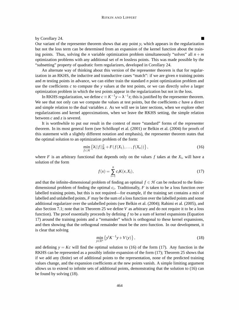
It is worthwhile to put our result in the context of more “standard” forms of the representertheorem. In its most general form (see Scholkopf et al. (2001) or Belkin et al. (2004) for proofs ofthis statement with a slightly different notation and emphasis), the representer theorem states thatthe optimal solution to an optimization problem of the form:

minf∈H

λ|| f ||2K +F( f (X1), . . . , f (Xn))

, (16)

where F is an arbitrary functional that depends only on the values f takes at the Xi, will have asolution of the form

f (x) =n

∑i=1

ciK(x,Xi), (17)

and that the infinite-dimensional problem of finding an optimal f ∈ H can be reduced to the finite-dimensional problem of finding the optimal ci. Traditionally, F is taken to be a loss function overlabelled training points, but this is not required—for example, if the training set contains a mix oflabelled and unlabelled points, F may be the sum of a loss function over the labelled points and someadditional regularizer over the unlabelled points (see Belkin et al. (2004); Rahimi et al. (2005), andalso Section 7.1; note that in Theorem 25 we define V as arbitrary and do not require it to be a lossfunction). The proof essentially proceeds by defining f to be a sum of kernel expansions (Equation17) around the training points and a “remainder” which is orthogonal to these kernel expansions,and then showing that the orthogonal remainder must be the zero function. In our development, itis clear that solving

miny∈Rn

ytK−1y+V (y)

, (18)

and defining y = Kc will find the optimal solution to (16) of the form (17). Any function in theRKHS can be represented as a possibly infinite expansion of the form (17); Theorem 25 shows thatif we add any (finite) set of additional points to the representation, none of the predicted trainingvalues change, and the expansion coefficients at the new points vanish. A simple limiting argumentallows us to extend to infinite sets of additional points, demonstrating that the solution to (16) canbe found by solving (18).

464


7.1 Semi-supervised and Transductive Learning

In this section we discuss in detail the somewhat subtle relationships between semi-supervised,transductive and inductive learning, quadratic regularizers, and the representer theorem.

In standard usage, inductive and semi-supervised learning are viewed as problems of taking atraining set (fully labelled for the inductive case, partially unlabelled for the semi-supervised case)and learning a function that classifies new examples. In contrast, transductive learning is oftenviewed as the problem of predicting the labels at unlabelled points, given the locations of thosepoints in advance. It must be understood that this distinction is somewhat artificial, based on notionsof what we consider a function. In particular, given any transductive algorithm A , we obtain a semi-supervised algorithm for classifying new points by rerunning A with all points seen so far whenevera prediction is needed. From this bird’s-eye view, all problems about “out of sample” extensions fortransductive algorithms (see for example Bengio et al. (2003)) vanish. This is a perfectly legitimatesemi-supervised algorithm, in that it provides a function for computing the values at new points;however, because evaluating the function requires solving an optimization problem, many peopleare uncomfortable with this algorithm. At the present time, it seems that it is common usage in themachine learning community to accept predictive functions which are weighted sums of expansionsaround a fixed basis as legitimate semi-supervised solutions, but to reject predictive functions whichrequire solving optimization problems as being merely transductive algorithms. This viewpoint isin some sense arbitrary, but also reflects genuine computational concerns; for the remainder of thissection, we refer to transductive and inductive algorithms as the terms are commonly used.

Given an arbitrary transductive algorithm, it is possible to turn it into an inductive algorithm byembedding the optimization in an RKHS. An excellent example is manifold regularization Belkinand Niyogi (2003). As originally formulated, manifold regularization is defined only for points ona graph, and is therefore a transductive algorithm. In Belkin et al. (2004), the authors construct aninductive algorithm by considering the optimization problem:

miny∈Rm+n

λ1ytK−1y+λ2ytLy+V (yN)

, (19)

where we have n labelled and m unlabelled points, yN are the predicted values at (just) the labelledpoints, and L is the graph Laplacian of (all) the data. The term ytLy is an additional smoothnesspenalty on the predicted values that respects the notion that we expect the data to live on or neara low-dimensional manifold. By the standard representer theorem, solving the above optimizationis equivalent to finding a function with minimal sum of its RKHS norm and the “loss function”λ2ytLy+V (yN). Similar extensions of straightforward RKHS regularizers with additional penaltiesare known for time series (Rahimi et al., 2005) and structured prediction (Altun et al., 2005).8 Infact, whenever the additional regularization term is a quadratic form QL, we can view the semi-supervised algorithm as finding the optimal function in a data-dependent “warped” RKHS (seeSindhwani et al. (2005) for details).

While we certainly agree that Problem 19 gives a finite-dimensional solution to an infinite-dimensional problem, we question whether this problem is the “right” problem to solve. In particu-lar, we consider two “strategies” for classifying new points:

8. We have not seen many examples in the machine learning literature of researchers treating the outputs y as thepredictive values. The above algorithms are generally phrased in terms of c, or sometimes in terms of f (x), with f (x)viewed as dependent on c.

465

RIFKIN AND LIPPERT

• (Inductive) Solve Problem 19. Compute c via y = Kc, yielding a “function” f (x) = ∑i ciK(x,xi).Use f to predict values at new points.

• (Transductive) When presented with a new point, compute an augmented form of optimiza-tion Problem 19 by adding the new point to the RKHS and additional regularization terms.Predict the value at the new point as the associated optimal value in the augmented optimiza-tion problem.

Given sufficient computational resources, we consider the transductive approach to be the “natural”choice, in that it treats previous and future unlabelled points on an equal basis. The inductive al-gorithm may be appropriate as a computationally more tractable substitute, but it is crucial to keepin mind that we do not expect the inductive and transductive approaches to give the same answer.This is in direct contrast to the case of standard RKHS supervised learning, where Theorem 25shows that the inductive and transductive approaches give the same answer. For RKHS supervisedlearning, unlabelled points do not contribute to the loss (we implicitly assume vi(yi) = 0 for unla-belled points). On the other hand, when we consider a data-dependent smoothness functional overunlabelled data, additional points give us additional information about this smoothness penalizer.In the transductive semi-supervised case, adding the unlabelled point to the optimization problemcan change the predictions at previous points, both labelled and unlabelled. We will see anotherexample of this phenomenon in Section 8.

An alternate perspective on problems like Problem 19 is to think of the smoothness penaltyQL(y) as part of the regularizer, rather than part of the loss. From this viewpoint, we no longer havea (data independent) RKHS regularizer, and so Theorem 25 does not apply.

8. Learning the Kernel

Standard RKHS regularization involves a fixed kernel function k and kernel matrix K. Recently,there has been substantial interest in scenarios in which a kernel matrix or kernel function is learnedfrom the data, simultaneously with learning a prediction function. We first develop some verygeneral results on this case, and then show how these results can easily be used to obtain andgeneralize results from the recent literature.

We consider a variant of Tikhonov regularization where the regularization term itself containsparameters u ∈ R

p, which are optimized; we learn the regularization in tandem with the regression.The primal becomes

infy,u

R(y,u)+∑i

vi(y)

.

where R(y,u) is convex in y. Given the independence of the loss from u, we can move the u-infimuminside

infy

infu

R(y,u)+∑i

vi(y)

obtaining a new regularization R′(y) = infu R(y,u). We will assume through the remainder thatR(y,u) is ccp.

466


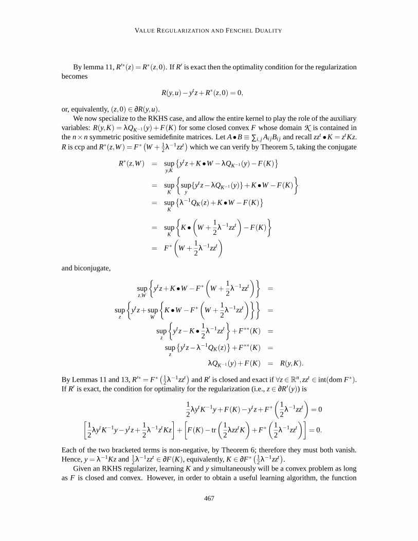
By lemma 11, R′∗(z) = R∗(z,0). If R′ is exact then the optimality condition for the regularizationbecomes

R(y,u)− ytz+R∗(z,0) = 0,

or, equivalently, (z,0) ∈ ∂R(y,u).We now specialize to the RKHS case, and allow the entire kernel to play the role of the auxiliary

variables: R(y,K) = λQK−1(y)+ F(K) for some closed convex F whose domain K is contained inthe n×n symmetric positive semidefinite matrices. Let A•B ≡ ∑i, j Ai jBi j and recall zzt •K = ztKz.R is ccp and R∗(z,W ) = F∗ (

W + 12 λ−1zzt

)

which we can verify by Theorem 5, taking the conjugate

R∗(z,W ) = supy,K

ytz+K •W −λQK−1(y)−F(K)

= supK

supyytz−λQK−1(y)+K •W −F(K)

= supK

λ−1QK(z)+K •W −F(K)

= supK

K •(

W +12

λ−1zzt)

−F(K)

= F∗(

W +12

λ−1zzt)

and biconjugate,

supz,W

ytz+K •W −F∗(

W +12

λ−1zzt)

=

supz

ytz+ supW

K •W −F∗(

W +12

λ−1zzt)

=

supz

ytz−K • 12

λ−1zzt

+F∗∗(K) =

supz

ytz−λ−1QK(z)

+F∗∗(K) =

λQK−1(y)+F(K) = R(y,K).

By Lemmas 11 and 13, R′∗ = F∗ (

12 λ−1zzt

)

and R′ is closed and exact if ∀z ∈ Rn,zzt ∈ int(dom F∗).

If R′ is exact, the condition for optimality for the regularization (i.e., z ∈ ∂R′(y)) is

12

λytK−1y+F(K)− ytz+F∗(

12

λ−1zzt)

= 0[

12

λytK−1y− ytz+12

λ−1ztKz

]

+

[

F(K)− tr

(

12

λzztK

)

+F∗(

12

λ−1zzt)]

= 0.

Each of the two bracketed terms is non-negative, by Theorem 6; therefore they must both vanish.Hence, y = λ−1Kz and 1

2 λ−1zzt ∈ ∂F(K), equivalently, K ∈ ∂F∗ (

12 λ−1zzt

)

.Given an RKHS regularizer, learning K and y simultaneously will be a convex problem as long

as F is closed and convex. However, in order to obtain a useful learning algorithm, the function

467

RIFKIN AND LIPPERT

F must provide a meaningful constraint on allowable kernels, and there must be a mechanism forpredicting values at new points. Abusing notation, let FN and FM be the versions of F that operate onn×n and m×m matrices, respectively (we usually suppress this notation). Suppose that, wheneverm > n, we have the property that FN(A) = infK:KNN=A FM(K). In this case, it is straightforward tosee that adding additional “testing” points to the regularizer, but not the loss, will not change theobjective value, nor will it change the y values at the “training” points. This leads to a transductivealgorithm. Furthermore, if the minimizer in the inf is unique, we can use KN to determine KM giventhe new x points, we will have a representer theorem, and the inductive and transductive cases willbe identical.

Lanckriet et al. (2004) consider a transductive scenario, where the training and testing pointsare known in advance. They start with a finite set of kernels K1, . . . ,Kk (the Ki are over the trainingand testing sets) and take F(K) = δKu,c(K), where

Ku,c ≡

K : K = ∑i

uiKi, tr(K) = c, K 0

.

(Lanckriet et al. (2004) frequently consider Ku+,c as well, where the u are constrained to be nonnega-tive.) A primary concern in Lanckriet et al. (2004) is showing that when the SVM hinge loss is used,the resulting optimizations can be phrased as semidefinite programming problems. They recognizethat it is important to “entangle” the training and testing kernel matrices—if we simply allowed Kto range over the entire semidefinite cone, for example, we would obtain kernel matrices which fitthe training data well and ignored the testing data. Using a finite combination of kernel matrices es-sentially means that we are learning a kernel function parametrized by u, and applying this functionto both training and testing points. Because Lanckriet et al. (2004) constrain the trace of the entirekernel matrix K, adding additional testing points can change the value at training points, and theycannot easily and directly perform induction. If they had instead chosen to constrain the trace of thekernel matrix over only the training points, or simply to constrain the sum of the ui, they could haveobtained a representer theorem, and there would have been agreement between their transductivealgorithm and the obvious inductive algorithm. Lanckriet et al. (2004) focus primarily on the SVMhinge loss. In fact, any convex loss can be used, and the resulting optimization problem can be castas a semidefinite programming problem (Recht, 2006).

While Lanckriet et al. (2004) consider a finitely generated set of kernel matrices, Argyriou et al.(2005) works with a convex set generated by an infinite, continuously parametrized set of kernelfunctions, the primary example being Gaussian kernels with all bandwidths in some closed interval.Argyriou et al. (2005) show that the optimal kernel function will have a “representation” in terms ofn+1 basic kernels. Because we have separated our concerns with the kernel function appearing onlyin the regularization and not in the loss, we are able to give a very simple proof of their result. Givena subset, K , of the n× n symmetric positive semidefinite matrices, we consider F(K) = δK ⊕(K),where K ⊕ is the convex hull of K .

Lemma 26 Let z ∈ Rn and K ∈ K ⊕. There exists K = ∑n+1

i=1 tiKi with ti ≥ 0 and ∑i ti = 1 such thatKz = Kz.

Proof Let Y = K ′z : K′ ∈ K and Y⊕ = K′z : K′ ∈ K ⊕. Clearly, Y⊕ is the convex hull of Y andKz ∈Y⊕. By Caratheodory’s theorem (Rockafellar and Wets (2004), Theorem 2.29), ∃t ∈R

n+1, ti ≥0,∑i ti = 1 such that Kz = ∑i tiyi with yi ∈ Y and hence yi = Kiz for some Ki ∈ K .

468


F∗ = σK ⊕ . Let us assume that K ⊕ is closed (compactness of K is sufficient but not necessary).Under this assumption, F is ccp, and the optimality condition from the regularization term becomes

y = λ−1Kz and ztKz = σK ⊕(zzt),K ∈ K ⊕. (20)

Corollary 27 Let z ∈ Rn,K ∈ K ⊕ and K ∈ K ⊕ be as in Lemma 26. If y,z,K satisfy (20) then y,z, K

do. Additionally, if ti > 0 then ztKiz = σK ⊕(zzt).

Proof The first claim comes directly from Kz = Kz. The second claim comes from ztKz = σK ⊕(zzt)and a standard argument.Since K does not appear in the loss optimality conditions (which depend only on z and y), we seethat we can construct an optimal y, K, and z for the entire kernel learning problem where K isa convex combination of at most n + 1 “atoms” of K that solve the problem. Our result is bothsubstantially simpler than the result of Argyriou et al. (2005), and more general in that it appliesto arbitrary convex loss functions: Argyriou et al. (2005)’s argument was essentially a saddle pointargument which required differentiability of the loss.

Our work generalizes previous results in this field, in that we have shown that one may usean arbitrary kernel penalizer F(K); previous work has used only δ functions. Exploring alternatepenalizers and developing algorithms is a topic for future work.

9. Regularizations and Bias

In this section, we consider relaxing primal regularizations by means of infimal convolutions. Theprimary application is unregularized bias terms for kernel machines. In Section 9.1, we obtain verygeneral results for biased regularizations, independent of particular loss functions and even partic-ular regularizers. In Section 9.2, we use similar techniques to analyze leave-one-out computationsfor RKHS learning.

9.1 Learning with Bias

So far, we have considered regularization in an RKHS, deriving formulations of regularized leastsquares and an unbiased version of the support vector machine. In practice, the SVM is generallyused with an unregularized bias term b (Poggio et al., 2001). This gives the regularization theproperty that R(y + b1n) = R(y)—constant shifts of the regression values are free. This can beachieved by taking a base regularization such as R = λQK−1 and replacing it with R′ = λQK−1 ?δ1nR

where 1n ∈ Rn is the vector of all 1s. In this case, we will see that the subgradient relation for the

regularization becomes

z ∈ ∂R′(y) ⇔(

λ−1K 1n

1tn 0

)(

zb

)

=

(

y0

)

, (21)

which relates y to both z and the bias parameter b.We examine biased regularizations more generally. Without loss of generality, we cast this

theorem in terms of an infimal convolution in the primal regularization, though by biconjugation,this lemma applies symmetrically to the primal and dual.

469

RIFKIN AND LIPPERT

Lemma 28 (bias) Let C ⊂ Rn be a closed convex set containing 0. Let R : R

n → (−∞,∞] be ccpwhere R′ = R?δC is exact. Then z ∈ ∂R′(y) iff ∃c ∈C such that

∀c′ ∈C,zt(c′− c) ≤ 0

R(y− c)− (y− c)tz+R∗(z) = 0. (22)

Proof By Theorem 15, z ∈ ∂R′(y) iff ∃c such that z ∈ ∂δC(c) and z ∈ ∂R(y− c). The first conditionis given by Equation 13, and the second condition is the generic condition of Theorem 6.The first condition in Lemma 28 is a normality condition on z taking different forms depending onthe geometry of C. It states that the hyperplane given by Hz,σC(z)(y) = 0 is a supporting hyperplaneof C. For example, if the boundary of C were smooth, then this condition reduces to z being anormal to C at c. If C = B, then z = λc for some λ ≥ 0.

If C is a vector subspace, then σC = δC⊥ , and (22) becomes the condition z ∈ C⊥ with c anarbitrary element of C. Thus, it seems worthwhile to specialize to the case of vector subspaces.

Corollary 29 Let V1 ⊂ V2 ⊂ Rn be vector subspaces. Let R : R

n → (−∞,∞] be ccp. Let R′ = R ?δV1 +δV2 . Then R′∗ = R∗ ?δV⊥

2+δV⊥

1and (assuming exactness of the ?’s) z ∈ ∂R′(y) iff y ∈V2,z ∈V⊥

1

and z−a ∈ ∂R(y−b) for some a ∈V⊥2 ,b ∈V1.

Proof Let R1 = R?δV1 and R2 = R1 +δV2 . By Lemma 28,

z1 ∈ ∂R1(y1) ⇔ z1 ∈V⊥1 and ∃b ∈V1 s.t. z1 ∈ ∂R1(y1 −b)

z2 ∈ ∂R2(y2) ⇔ y2 ∈V2 and ∃a ∈V⊥2 s.t. z2 −a ∈ ∂R1(y2).

Thus,

z ∈ ∂R′∗(y) ⇔ y ∈V2 and ∃a ∈V⊥2 s.t. z−a ∈V⊥

1

and ∃b ∈V1 s.t. z−a ∈ ∂R(y−b)

⇔ y ∈V2 and z ∈V⊥1 and ∃a ∈V⊥

2 ,b ∈V1 s.t. z−a ∈ ∂R(y−b),

where the last line is due to V⊥2 ⊂V⊥

1 .

Suppose we start with a regularization R, and we wish to allow a free constant bias in the yvalues. Our primal problem is:

infy,b

R(y−b1n)+n

∑i=1

(1− yiYi)+

= infy

(R?δ1nR)(y)+n

∑i=1

(1− yiYi)+

.

In the dual, the regularization term becomes (R∗ + δ(1nR)⊥)(z). We see that the dual regularizer

z ∈ (1nR)⊥ can also be written as the constraint ∑zi = 0. We have shown that for any regularizationand loss function, allowing a free unregularized constant b in the y values induces a constraint∑i zi = 0 in the dual problem. Nothing else changes: to obtain the standard “biased” SVM insteadof the unbiased SVM we derived in Section 5.2.2, we change the primal regularizer from QK−1

to QK−1 ? δ1nR, we change the dual regularizer from QK to QK + δ(1nR)⊥ , or, equivalently, we addthe constraint ∑i zi = 0 to the dual optimization problem. There is no need to take the entire dualagain—the loss function is unchanged, and in the Fenchel formulation, the regularization and lossmake separate contributions.

470


In terms of Corollary 29, the standard constant bias is obtained by choosing V1 = 1nR,V2 = Rn,

and therefore a = 0 and R?δV1 +δV2 = R?δV1 . Assuming we are using an RKHS primal regularizerQK−1 , then z ∈ ∂(QK−1 ?δV1)(y−b) iff b ∈ 1nR and z ∈ ∂QK−1(y−b), or, equivalently, if (21) holds.

We can incorporate the same bias into regularized least squares. Recalling that the loss opti-mality condition for RLS is y+ z = Y , we can eliminate either y or z from the optimality condition,obtaining either a pure primal or pure dual formulation for the so-called least squares SVM (Suykenset al., 2002).

(

λ−1K 11t 0

)(

Yi

b

)

=

(

I +λ−1K 11t 0

)(

y0

)

(

I +λ−1K 11t 0

)(

zb

)

=

(

Yi

0

)

,

Note that introducing biases via infimal convolutions with RKHS regularization preserves therepresenter property:

Corollary 30 Let K =

(

KNN KNM

KMN KMM

)

∈R(n+m)×(n+m) be symmetric positive definite where KNN ∈

Rn×n. Let C ∈ R

n+m be a closed convex set containing 0, and let CN be the projection of C onto thefirst N dimensions. For all y1 ∈ R

n,

infy2∈Rm

(QK−1 ?δC)(y1,y2) = (QK−1NN

?δCN )(y1),

where the minimizer is of the form y2 = KMNK−1NN(y1 − c1)+ c2 where (c1,c2) ∈C.

Proof

infy2∈Rm

(QK−1 ?δC)(y1,y2) = infy2∈Rm

inf(c1,c2)∈C

QK−1((y1,y2)− (c1,c2))

= inf(c1,c2)∈C

infy2∈Rm

QK−1((y1,y2)− (c1,c2))

= infc1∈CN

infy′2∈Rm

QK−1(y1 − c1,y′2)

= infc1∈CN

QK−1NN

(y1 − c1),

where the last equality is an application of Corollary 24 (the statement about y2 then follows sincethat QK−1 ?δC and QK−1

NN?δCN are exact).

The minimizing y2 will be unique if a transversality condition holds: ∀(c1,c2),(c′1,c′2) ∈ C,c1 =

c′1 ⇒ c1 = c′2. For the standard constant-term bias, this is clear and the recovery of y2 reduces toy2 = KMNK−1

NN(y1 −1nb)+1mb.

9.2 Leave-one-out Computations

For small data sets, it is frequently of interest to do model selection via leave-one-out cross valida-tion. Done naively, this involves solving n optimization problems, one for each size n−1 subset ofthe data, and testing n− 1 functions at the remaining points. In this section, we relate the solutionof the full problem (using all the data points) to the leave-one-out value.

471

RIFKIN AND LIPPERT

We consider an n+1 point data set, and define y = (y0,yN) ∈ Rn+1 in a regression problem with

losses vi(y) for 0 ≤ i ≤ n. The “full” optimization problem, with an RKHS regularization, is

infy∈Rn+1

λQK−1(y)+n

∑i=0

vi(yi)

.

We now show how we can compute a “leave one out” score as the auxiliary variable of a biasedregularization of the form δC where C = (y0,0) ∈ R

n+1. Consider the optimization,

infy∈Rn+1

λ(QK−1 ?δC)(y)+n

∑i=0

vi(yi)

= infy∈Rn+1,β∈R

λQK−1(y−βe0)+n

∑i=0

vi(yi)

.

By Corollary 29, the right hand problem has the regularization optimality condition

(

λ−1K e0

et0 0

)(

zβ

)

=

(

y0

)

,

Clearly, at optimality, z0 = 0 and y0 will assume a value with minimal loss: v0(y0) = infy v(y) ≡ v.With z0 = 0, it is clear that the values z1, . . . ,zn and y1, . . . ,yn are an optimal solution to the restrictedproblem obtained by simply discarding (X0,Y0), and that therefore, (λ−1Kz)0 is the value we wouldobtain if we solved the restricted problem and computed the “test value” at X0. β is the leave-one-out“error” y0 − (λ−1Kz)0.

In the case of a square loss, the loss optimality conditions are z+y =Y , allowing us to eliminatey,

(

I +λ−1K e0

et0 0

)(

zβ

)

=

(

Y0

)

,

and solve for β, Defining G ≡ I +λ−1K, we have

β =et

0G−1Y

et0G−1e0

,

the standard formula for RLS leave-one-out errors.

10. Low-rank Approximation of Kernel Matrices

Given n data points, the kernel matrix K is n by n. For large n, it is impractical to compute with(or store) K. Consequently, there has been an interest in approximations to K. In this section,we consider a class of low rank approximations to K obtained by considering a vector subspaceV0 ⊂ R

n, and defining K as the lowest rank symmetric matrix such that KV0 = KV0. The primaryexample is the well-known Nystrom approximation (Baker, 1977). When the Nystrom kernel matrixapproximation was first used in machine learning applications (Willams and Seeger, 2000), thesuggested approach was to simply replace K with K; we refer to this approach as the Nystrommethod. We will show that the “natural” algorithm suggested by the Nystrom approximation is infact the subset of regressors method (Poggio and Girosi, 1990; Luo and Wahba, 1997), as opposed

472


to the Nystrom method.9 In contrast, the Nystrom method essentially makes an unwarranted (andincorrect) assumption that the representer theorem, which directly connects the dual variables z andthe function expansion coefficients c in the standard RKHS case, still holds when we replace K withK. Our observation is consonant with empirical reports (Rifkin, 2002; Rasmusen and Williams,2006) that the subset of regressors algorithm tends to outperform the Nystrom algorithm. We notein passing that whereas previous algorithmic work with the Nystrom approximation has mostlyfocussed on Gaussian Process regression or regularized least-squares, our results are all independentof the particular loss function chosen.

We first show that QK has a simple characterization.

Lemma 31 Let K, K ∈ Rn×n with K symmetric positive definite and KV0 = KV0 with rank(K) =

dimV0. Then QK = QK ?δ(KV0)⊥ .

Proof For all v ∈ V0 and n ∈ Null(K), 0 = ntKv = ntKv, thus, since rank(K) = dimV0, Null(K) =(KV0)

⊥ and V0 ∩ (KV0)⊥ = 0.

Given v ∈V0,n ∈ (KV0)⊥,

QK(v+n) =12(v+n)tK(v+n)

= QK(v)+QK(n)

QK(v+n) = (v+n)tK(v+n)

=12

vtKv =12

vtKv = QK(v).

In comparison

(QK ?δ(KV0)⊥)(v+n) = infw

QK(v+n−w)+δ(KV0)⊥(w)

= QK(v)+ infw∈(KV0)⊥

QK(n−w)

= QK(v).

Lemma 31 implies

infz

λ−1QK(z)+V ∗(−z)

= infz

λ−1(QK ?δ(KV0)⊥)(z)+V ∗(−z)

= infz∈Rn,z′∈(KV0)⊥

λ−1QK(z− z′)+V ∗(−z)

= infz′′∈Rn

λ−1QK(z′′)+ infz′∈(KV0)⊥

V ∗(−z′′− z′)

. (23)

We see that giving the regularization a non-trivial nullspace ((KV0)⊥) is equivalent to allowing an

unregularized “bias” from that same space. Hence, we expect the resulting modified dual optimiza-tion problem to have a lower value than the original dual.

9. To avoid confusion, we reiterate that the Nystrom approximation is a low-rank approximation to K, denoted by K,while the Nystrom method is obtained by simply replacing K with K in an algorithm such as regularized least squares.

473

RIFKIN AND LIPPERT

The modified primal problem, the Fenchel dual of (23), is

infyλQK−1(y)+δKV0(y)+V (y) = inf

y∈KV0λQK−1(y)+V (y) (24)

which is identical to the original optimization problem, but with a restricted domain, and hence ahigher value, in general. This is to be expected, as any pair of Fenchel duals have inversely relatedinfimal values. For the remainder of this section, the variables y and z refer, respectively to optimalsolutions to the modified primal (24) and dual (23) problems.

So far, we have considered an arbitrary subspace V0. We now specialize to the Nystrom approx-

imation, obtained by partitioning the data into two blocks N and M with K =

(

KNN KNM

KMN KMM

)

, and

taking V0 =

(

I0

)

Rn, in which case

K =

(

KNN KNM

KMN KMNK−1NNKNM

)

=

(

I 0KMNK−1

NN 0

)(

KNN KNM

KMN KMM

)

.

It is obvious that KV0 = KV0 and the expression on the right demonstrates that K is rank n.

By Corollary 29, with V2 = K

(

I0

)

Rn =

(

K−1

(

0I

)

Rm

)⊥and V1 = 0, the complementarity

relation between y and z due to the regularization terms of the modified problems (24) and (23) is

(

z0

)

= λ

K−1 K−1

(

0I

)

(0 I )K−1 0

(

yα

)

or, equivalently, ∃r ∈ Rn such that

y = λ−1K

(

r0

)

(25)

and

λ−1Kz = y+

(

0α

)

(26)

λ−1Kz = y, (27)

where (27) is obtained from (26) by multiplying the first equation on the left by

(

I 0KMNK−1

NN 0

)

and observing that K

(

r0

)

= K

(

r0

)

by construction.

In standard Tikhonov regularization in an RKHS, the complementarity equation from the regu-larization, y = λ−1Kz, and the representer theorem tells us that we can obtain an optimizing functionusing c = λ−1z. Once we have replaced K with K, this connection no longer holds, and we mustdecide how to generalize a minimizer of (23) or (24) into a function that can be used to predictthe values at future points. The Nystrom method, suggested in Willams and Seeger (2000) is touse the function fd(x) ≡ ∑n+m

i=1 λ−1zik(x,Xi), essentially “pretending” that the connection between c

474


and z is still valid. An alternate choice is to use r, yielding fp(x) ≡ ∑ni=1 λ−1rik(x,Xi).10 By (26),

fp(Xi) = fd(Xi) when 1 ≤ i ≤ n, while fd(Xi) = fp(Xi)+αi−n when n < i ≤ n+m—the two regres-sors are related, taking the same values at the first n points but generally different values on the lastm points.

By eliminating y for r in the modified primal problem (24), we see that f p is the solution of thesubset of regressors method, where we construct a function using only those coefficients associatedwith points in N:

infy∈KV0

λQK−1(y)+V (y) = infr∈Rn

λ−1QKNN (r)+V

(

λ−1(

KNN

KMN

)

r

)

.

In this sense, we can see that the subset of regressors method is associated with the modified prob-lems (24) and (23). Additionally, the function fp will recover the y values optimizing (24) at alln + m training points. In contrast, if we use the Nystrom method on the last m training points, wewill not recover the last m values—they will differ by α.

We have shown that the subset of regressors method corresponds in a natural way to the modifiedprimal and dual problems obtained by replacing K with the Nystrom approximation K, whereas theNystrom method makes the additional unwarranted assumption that it is still a good idea to constructa function to classify future points using c = λ−1z. We can also derive an interesting relationshipbetween the functions fp and fd .

We first note that by (25), y and

(

0α

)

are “K−1 orthogonal”: ytK−1

(

0α

)

=

(

r0

)t ( 0α

)

= 0.

As a consequence, the quadratic form QK−1 “distributes” over y and

(

0α

)

:

QK−1(λ−1Kz) = QK−1

(

y+

(

0α

))

= QK−1(y)+ ytK−1(

0α

)

+QK−1

(

0α

)

= QK−1(y)+QK−1

(

0α

)

.

Furthermore, by (26),

(

0α

)t

z =

(

0α

)t ((

r0

)

+λK−1(

0α

))

= λ(

0α

)t

K−1(

0α

)

= 2λQK−1

(

0α

)

.

We now consider comparing the functions fd and fp. Recall that the values of fd at all training pointsare equal to λ−1Kz while those of fp are y. Because y and z are optimal solutions to the modified

10. We chose the name fd and fp because the two functions seem to us “suggested” by the modified dual and primalproblems, respectively.

475

RIFKIN AND LIPPERT

primal and dual problems, −z ∈ ∂V (y). Since −z is a subgradient of V at y, V (y)−zt(y′−y)≤V (y′)

for all y′ ∈ Rn. Setting y′ = λ−1Kz, and noting that λ−1Kz− y =

(

0α

)

, by (26), we have,

V (y)−V (y′) ≤ zt(y′− y) = zt(

0α

)

= 2λ(

QK−1(λ−1Kz− y))

= 2λ(

QK−1(y′)−QK−1(y))

= 2λQK−1

(

0α

)

.

Recall that y was obtained by minimizing V (y) + λQK−1(y) over KV0. Comparing the functionvalues y and y′ of the regressors fp and fd respectively, we see that fd pays a higher regularization

cost as compared to fp, QK−1(y′)−QK−1(y) = QK−1

(

0α

)

. Furthermore, the difference in loss at the

last m points in favor of fd is bounded by 2λ times this difference—it is not possible for fd to havearbitrarily smaller loss. In practice, we often find that the Nystrom method produces worse functionvalues at the m points than the subset of regressors does. This provides further evidence that thesubset of regressors method should be preferred to the Nystrom method.

11. Discussion and Future Work

We have introduced a new framework for thinking about optimization in learning theory by com-bining two key elements: Fenchel duality and value regularization. Fenchel duality allows us toanalyze the optimality conditions for regularization and loss terms separately, and combine theseoptimality conditions to get complete optimality conditions for machine learning schemes. Valueregularization makes it easy to reason about optimization problems over training and testing pointssimultaneously, and isolates the RKHS kernel to the regularization term. We have used the frame-work to gain new insights into several topics in machine learning, including the representer theorem,learning a kernel matrix, biased regularizations, and low-rank approximations to kernel matrices.There remain several interesting open questions.

In Sections 7 and 8, we showed that both supervised learning in an RKHS and learning the ker-nel matrix had a representer theorem that caused the inductive and natural transductive algorithmsto make the same prediction. It would be interesting to explore this idea further, characterizingformally what sorts of conditions give rise to agreement between inductive and transductive algo-rithms.

The framework developed in this article is specialized to the case where the predicted outputsy are real-valued scalars. It is frequently of interest to make predictions on objects with morestructure: examples include multiclass classification, ranking, and classification of sequences. Theextension of the value regularization framework to these problems is in principle straightforward,but many details remain to be worked out.

Finally, although this article has focussed on the analysis of existing schemes, one may askwhether a value regularization perspective can lead to the development of new learning algorithms.It seems unlikely that value regularization in an RKHS will lead directly to improved algorithms(for example, a better SVM solver), because the inverse kernel matrix K−1 appearing in the primalis a computationally inconvenient object. However, we might imagine designing regularizers forwhich value-based optimization is computationally effective, such as a transductive algorithm with a

476


regularizer that directly imposes some non-RKHS smoothness over the input space. We are activelyworking to design and implement such algorithms.

Acknowledgments

We thank Ben Recht, Tomaso Poggio, Rob Freund, Adrian Lewis and Roger Wets for helpful dis-cussions and suggestions. We thank Gustavo Santos and Tim Sears for finding many technical errorsin earlier versions of this work. We thank our anonymous reviewers for helpful suggestions.

References

Yasemin Altun and Alex Smola. Unifying divergence minimization and statistical inference viaconvex duality. In Proceedings of the 19th Annual Conference on Lwearning Theory, 2006.

Yasemin Altun, David McAllester, and Mikhail Belkin. Maximum margin semi-supervised learningfor structured variables. In Neural Information Processing Systems, 2005.

Andreas Argyriou, Charles A. Micchelli, and Massimiliano Pontil. Learning convex combinationsof continuously parametrized basic kernels. In Proceedings of the 18th Annual Conference onLearning Theory, 2005.

Nachman Aronszajn. Theory of reproducing kernels. Transactions of the American MathematicalSociety, 68:337–404, 1950.

Christopher T. H. Baker. The Numerical Treatment of Integral Equations. Clarendon press, 1977.

Mokhtar S. Bazaraa, Hanif D. Sherali, and C. M. Shetty. Nonlinear Programming: Theory andAlgorithms. Wiley-Interscience, 2nd edition, 1993.

Mikhail Belkin and Partha Niyogi. Semi-supervised learning on riemannian manifolds. MachineLearning, 56:209–239, 2003.

Mikhail Belkin, Partha Niyogi, and Vikas Sindhwani. Manifold regularization: A geometric frame-work for learning from examples. Technical Report TR-2004-06, University of Chicago, 2004.

Yoshua Bengio, Jean-Francois Paiement, Pascal Vincent, Olivier Delalleau, Nicolas Le Roux, andMarie Ouimet. Out-of-sample extensions for LLE, Isomap, MDS, eigenmaps and spectral clus-tering. In Neural Information Processing Systems, 2003.

Jonathan M. Borwein and Adrian S. Lewis. Convex Analysis and Nonlinear Optimization. CMSBooks in Mathematics. Springer, 2000.

Scott Shaobing Chen, David L. Donoho, and Michael A. Saunders. Atomic decomposition by basispursuit. Technical Report 479, Stanford University Department of Statistics, 1995.

Corinna Cortes and Vladimir Vapnik. Support vector networks. Machine Learning, 20:1–25, 1995.

Nello Cristianini and John Shaw-Taylor. An Introduction To Support Vector Machines. CambridgeUniversity Press, 2000.

477

RIFKIN AND LIPPERT

Miroslav Dudık and Robert E. Schapire. Maximum entropy distribution estimation with generalizedregularization. In Proceedings of the 19th Annual Conference on Lwearning Theory, pages 123–138, 2006.

Theodoros Evgeniou, Massimiliano Pontil, and Tomaso Poggio. Regularization networks and sup-port vector machines. Advances In Computational Mathematics, 13(1):1–50, 2000.

Federico Girosi. An equivalence between sparse approximation and support vectomachines. NeuralComputation, 10:1455–1480, 1998.

Tommi S. Jaakkola and David Haussler. Probabilistic kernel regression models. In Proceedings ofthe 1999 Conference on AI and Statistics. Morgan Kaufmann, 1999.

Gert R. G. Lanckriet, Nello Cristianini, Peter Bartlett, Laurent El Ghaoui, and Michael I. Jordan.Learning the kernel matrix with semidefinite programming. Journal of Machine Learning Re-search, 5:24–72, 2004.

Zhen Luo and Grace Wahba. Hybrid adaptive splines. Journal of the American Statistical Society,92:107–116, 1997.

Charles A. Micchelli. Interpolation of scattered data: distance matrices and conditionally positivefunctions. Constructive Approximation, 2(1):11–22, 1986.

Tomaso Poggio and Federico Girosi. Networks for approximation and learning. Proceedings of theIEEE, 78(9):1481–1497, September 1990.

Tomaso Poggio, Sayan Mukherjee, Ryan M. Rifkin, Alex Rakhlin, and Alessandro Verri. b. InProceedings of the Conference on Uncertainty in Geometric Computations, 2001.

Ali Rahimi, Benjamin Recht, and Trevor Darrell. Learning appearance manifolds from video. InComputer Vision and Pattern Recognition, 2005.

Carl Edward Rasmusen and Chris Williams. Gaussian Processes for Machine Learning. MIT Press,2006.

Ben Recht. Unpublished phd thesis. 2006.

Ryan M. Rifkin. Everything Old Is New Again: A Fresh Look at Historical Approaches to MachineLearning. PhD thesis, Massachusetts Institute of Technology, 2002.

R. Tyrrell Rockafellar and Roger J. B. Wets. Variational Analysis. Springer, Berlin, 2004.

Bernhard Scholkopf, Ralf Herbrich, and Alex J. Smola. A generalized representer theorem. In 14thAnnual Conference on Computational Learning Theory, pages 416–426, 2001.

Vikas Sindhwani, Partha Niyogi, and Mikhail Belkin. Beyond the point cloud: from transductiveto semi-supervised learning. In Proceedings of the 22nd International Conference on MachineLearning, 2005.

Johan A. K. Suykens, Tony Van Gestel, Jos De Brabanter, Bart De Moor, and Joos Vandewalle.Least Squares Support Vector Machines. World Scientific, 2002.

478


Andrei N. Tikhonov and Vasilii Y. Arsenin. Solutions of Ill-posed problems. W. H. Winston, Wash-ington D.C., 1977.

Vladimir Vapnik. Statistical Learning Theory. John Wiley & Sons, 1998.

Grace Wahba. Spline Models for Observational Data, volume 59 of CBMS-NSF Regional Confer-ence Series in Applied Mathematics. Society for Industrial & Applied Mathematics, 1990.

Christopher K. I. Willams and Matthias Seeger. Using the Nystrom method to speed up kernelmachines. In Advances in Neural Information Processing Systems, 2000.

Ji Zhu, Saharon Rosset, Trevor Hastie, and Rob Tibshirani. 1-norm support vector machines. InNeural Information Processing Systems, 2003.

479

Documents

Value Regularization and Fenchel Dualityjmlr.csail.mit.edu/papers/volume8/rifkin07a/rifkin07a.pdf · the combination of value regularization and Fenchel duality are valuable tools