1

Valuation of public investment to support bicycling Beat Hintermann, University of Basel and CESifo

Thomas Götschi, University of Zurich

(Version: January 17, 2013)

Abstract

In this paper we develop a framework to value public investments with the purpose of increasing

bicycling that explicitly accounts internal costs of bicycling, which are typically neglected in

current established approaches that value bicycle spending by means of gross health benefits

alone, as are inframarginal benefits to existing cyclists. By monetizing internal costs independent

of health benefits, we can assess the degree of internalization of private benefits and/or the

internalization of external benefits such as environmental improvements due to altruistic

preferences by cyclists. Our framework further conceptualizes the complementarity between

“hard” (investments in infrastructure) and “soft” measures (informational campaigns) in bicycle

policy. Finally, we propose an empirical method for identifying internal costs using a latent

variable approach and apply it to eight Swiss cities. Our results imply that Swiss cyclists

internalize more than mortality-based benefits. However, because data for some important

bicycle mode choice determinants are not available, our results cannot inform policy directly at

the current stage. Instead, the contributions of our paper are the development of an economically

consistent framework to value public bicycle investments and the identification of crucial data

needs for the development of comprehensive assessments informing bicycle policy decisions.

JEL H43, H76; Q51; R41, R42.

Declaration of funding sources: We are grateful for financial support for this research from the

WWZ Forum, Basel, Switzerland.

2

1. Introduction

Transport agencies in many large cities in industrialized countries, and many regional and federal

governments, have offices responsible for designing and carrying out bicycle-friendly policies,

usually in coordination with other planning activities such as road construction or public

transportation. The role of government to design and finance bicycle policies can be justified by

the public-good characteristic of bicycle infrastructure and the substantial fixed costs, but also by

net beneficial effects associated with bicycling compared to other modes of transportation, such

as a reduction in mortality and morbidity due to increased physical activity, reduction of

congestion, and reduction in air pollution (Woodcock et al., 2009). Public interventions to

increase the level of bicycling have often been successful, implying that policy has an important

role when it comes to bicycling as a mode of transportation (Pucher et al., 2010). Although

public funds allocated to bicycle policies rarely exceed a few percent of the total transportation

budget, studies quantifying benefits indicate excellent benefit-cost—ratios for cycling

interventions (Cavill et al., 2009; Gotschi, 2011; Krizek et al., 2007; Wang et al., 2005).

However, economic decision criteria about bicycle-related investments are not well developed.

Progress has been made in terms of identifying the determinants of bicycle mode choice, in

assessing effectiveness of policy and infrastructure measures, and in the valuation of particular

costs and benefits of bicycling, but these different strands of research have not been integrated in

a framework suitable for an economically consistent cost-benefit analysis. This paper takes a

first step to fill this gap.

3

Our main contribution is the development of a conceptual as well as an empirical framework to

value bicycle-related policies1 that explicitly accounts for the internal costs of bicycling. Many

of the relevant costs and benefits associated with bicycling are intangible, such as disutility from

physical effort, inconvenience, fear of accidents, competition for crowded road space etc.

Considering the well-documented and significant health benefits from exercise associated with

bicycling, we argue that if it were not for such intangible net costs, the bicycle mode share for

short trips would be much higher than current levels in most countries.

Since intangible costs are not directly observable we rely on a latent variable approach, drawing

on results from the transportation mode choice literature to select indicator variables for internal

costs. Existing valuations of bicycle spending abstract from internal costs and implicitly assume

that the pre-intervention level of bicycling is given exogenously. Relative to this benchmark, our

framework leads to smaller net benefits for the additional bicycle-km (the increase in bicycling

due to the investment), but to additional benefits for inframarginal bicycle-km (bicycling taking

place already before the investment), which are not considered in existing valuations. The net

difference between our and existing approaches is ambiguous and depends on the context, but in

general our model leads to higher benefits at higher levels of bicycling.

As a second contribution, our model allows for an assessment of the degree of internalization of

health benefits or time savings. This is of interest because many existing analyses of cycling

imply health benefits of a magnitude which does not appear to be reflected in consumers’

choices. Along with internal costs, incomplete internalization of health benefits could be part of

an explanation for these seemingly “too low” levels of bicycling. It is also possible that

consumers consider some of the external effects of bicycling such as savings to the health care

1 We refer to bicycle policy in the broadest sense, including physical infrastructure but also any institutional and urban planning changes that affect the level of bicycling.

4

system or a reduction in air pollution (if bicycle-km substitute motorized transportation).2

Estimating the degree of internalization of health effects or other benefits requires an independent

monetization of internal costs. In the current paper we do this via money savings from bicycling

relative to public transportation, but alternative methods (e.g. savings relative to motorized

traffic, or stated preference surveys) could be used as well.

Our framework further allows to conceptualize one of the most pressing questions in promotion

of bicycling, that of interactive effects, or the optimal mix of so called “hard” and “soft”

measures. “Hard measures” (e.g. infrastructure) are aimed at reducing internal costs of bicycling.

Certain “soft measures” (informational and educational campaigns highlighting benefits of

bicycling) enable people to internalize them in their decision making. Hard and soft measures are

both considered vital ingredients to an effective mix of measures to promote bicycling (Pucher et

al., 2010), but to date there is no modeling approach available to quantify their individual and

synergistic effects, leaving it to policy makers’ best guesses to strike the optimal balance.

We apply our model to bicycling in eight Swiss cities using data from the Swiss Microcensus.

Our parameters are statistically significant and (mostly) have the expected sign, but due to data

and other limitations our results are sensitive to the inclusion of particular variables. The main

contribution of our paper is therefore conceptual. An application of the model to a richer data

context would be a fruitful avenue of future research.

The next section introduces our model and contrasts it to existing approaches from the literature.

Section 3 introduces the data, and Section 4 contains our econometric specification and presents

our empirical results. Section 5 concludes.

2 Neoclassical economic theory holds that consumers do not consider external effects, but recent research in behavioral and experimental economics implies that this may not be the case in the presence of commitment problems, pro-social preferences or reasons related to self-image (see e.g. Bernheim and Rangel, (2007) or Benabou and Tirole, (2006)

5

2. Valuation of bicycle policies

A key feature of any economic model is that people choose their actions according to their

preferences, conditionally on the set of available information. For bicycling, this means that

riders choose the level of bicycling that is optimal for them by weighing the internal costs and

benefits of bicycling against the existing alternatives. In the following we describe the most

important gross costs and benefits, and then turn to the issue of internal vs. external net costs.

2.1 Gross costs and benefits of bicycling

Bicycling is associated with a number of positive and some negative effects, and a literature has

developed on the subject with the aim of defining, quantifying and sometimes monetizing various

costs and benefits. In terms of magnitude, the most important effects are a.) decreased mortality

and morbidity as a result of physical activity, b.) increased injury risk as a result of exposure to

traffic environments, and c.) increased mortality and morbidity due to exposure to air pollutants

while riding in traffic (de Hartog et al., 2010; de Nazelle et al., 2011; Rojas-Rueda et al., 2011;

Woodcock et al., 2009).

With an assumption about substitution between bicycling and other means of transportation based

on empirical findings of substitution (Thakuriah et al., 2012), additional effects include d.)

reduced air pollution, noise and congestion, e.) lower demand for parking spaces, f.) less wear

and tear on roads, g.) time gain/loss during trips, or substituting for exercising in a gym, and h.)

intangible effects such as “livability” (Dumbaugh, 2005; Ellison and Greaves, 2011; Litman,

2004). With the exception of time savings, the substitution effects are borne not only by

bicyclists but the population as a whole.

This list is not meant to be exhaustive; its purpose is to illustrate the diversity of impacts, the

quantification and monetization of which requires contributions from various disciplines such as

6

epidemiology, physiology, urban planning, and last but not least economics.3 The literature on

(health) impact assessment of cycling has made progress along many of these lines of research by

improving the quality of individual pieces along causal pathways and reducing the number of

simplifying assumptions necessary to account for the lack of data and effect estimates, which

remains a pervasive problem in this area of research.4

Existing “gross health benefit” (GHB hereafter) valuations compute average benefits per unit of

bicycling and apply them to observed or projected increases in bicycling (e.g. Gotschi, 2011;

Saelensminde, 2004). However, most of these benefits accrue to bicyclists and should therefore

(at least partly) be internalized in people’s decision to bicycle when they trade off costs and

benefits. Equating such internal health benefits with net benefits, as is often done, amounts to

double-counting, as pointed out by Borjesson and Eliasson (2012). Whether internalization of

health benefits is complete is a different question that we address separately below; the point is

that the (implicit) assumption of zero internalization is most likely not correct. Separating

between internal and external benefits is crucial for the valuation of bicycle spending, as well as

for projecting the likely increase in bicycling as a result of bicycle promotion measures.

2.2 Internal costs of bicycling

Abstracting from leisure trips that serve no purpose of transportation, getting from A to B

conveys disutility to people in the form of money, time, and other costs. If there were only

positive health benefits (net of accident risks and increased exposure to air pollution), bicycling

3 Epidemiological studies are needed to estimate dose-response functions between physical activity and air pollution and the most relevant diseases, ideally by age, gender and activity types. Physiologists convert distance traveled by bicycle into exercise units, ideally by intensity (Ainsworth et al., 2000) Surveys are required to get an idea about the likely composition of the additional ridership. Finally, values of risk reduction derived from economic analyses, commonly referred to as the Value of a Statistical Life (VSL), are used to compute the benefits from reduced mortality, and sometimes this is further refined to take into account disability- or quality-adjusted life years. 4 See, e.g. de Geus et al., 2008; de Hartog et al., 2010; de Nazelle et al., 2011; Gotschi, 2011; Int Panis et al., 2010; Rojas-Rueda et al., 2011; Woodcock et al., 2009).

7

would be the dominant choice of transportation for all trips below a certain distance and at

moderate levels of accident risk.5 However, the bicycle mode share in Swiss cities is around 5%,

with few reaching more than 10% for all trip lengths (Federal Statistical Office, 2007, 2012).

There is a large literature devoted to identifying the determinants of transportation mode choices

in general, including bicycling. We reference key publications for selected determinants below

and refer to various additional studies for further evidence.6

We separate the determinants that have been empirically identified to affect the propensity to

bicycle into the following groups:

a.) Route characteristic which can potentially be influenced by city planners. Characteristics

shown to influence the amount of bicycling include the presence of bicycle lanes/paths; the

lane width, the volume and speed of motorized traffic; competition for space between drivers

and cyclists; the number of stops, traffic lights or other obstacles; the number of intersections

and their characteristics, accident risk; and qualitative aspects about bike lanes such as

continuity and connectivity or the presence of on-street parking. This category may also

include trip end facilities such as locking stations or the presence of showers at work (Dill,

2009; Lusk et al., 2011; Berrigan et al., 2010).

b.) External factors about the route that are treated as exogenous by planning authorities, at least

in the short or medium term. Such factors include weather (temperature and precipitation),

hilliness, city size, cultural and neighborhood characteristics including land use, and prices of

alternative modes of transportation.

5 Dutch cities and Copenhagen prove that there is no “law of nature” capping bicycle mode share anywhere close to what is observed in most cities without long history of systematic bicycle investments. 6 See e.g. Buehler and Pucher, 2012; Caulfield et al., 2012; Elston, 2002; Harris et al., 2011; Heinen and Handy, 2012; Hunt and Abraham, 2007; Kirner Providelo and Sanches, 2011; Menghini et al., 2009; Parkin et al., 2008; Plaut, 2005; Rietveld and Daniel, 2004; Sener et al., 2009; Smith, 1991; Troped et al., 2001; Vandenbulcke, 2011; Wardman et al., 2007; Xing et al., 2010.

8

c.) Personal characteristics of actual and potential (i.e. marginal) bicyclists, such as age, race,

gender, education, car ownership, aversion to driving, perception of bicycle-friendliness of

the traffic environment or environmental preferences (Heinen and Handy, 2012).

d.) Internal costs and benefits. Here we include items that affect the utility from bicycling

directly, such as psychological costs due to effort or fear of accidents, conflict with drivers,

inconvenience factors such as perspiration or problems with dress code etc, but also costs

from time loss relative to other modes of transport (time gains would be benefits). Some

mode choice studies explicitly consider this type of cost, whereas in the majority internal

costs are implicit.7 Smith (1991) finds that psychological costs of bicycling are a significant

predictor of bicycle mode choice. Similarly, Rietveld and Daniel (2004) report “generalized

costs” as a significant predictor variable, in which they include measures such as costs of

effort or fear of accidents, and Hunt and Abraham find that bicyclists choose routes that are

least “onerous”. Menghini et al. (2010) conclude that trip length is the dominant factor for

route choice, which is consistent with high time costs and/or costs of physical exertion.8

In our empirical model, we rely on some these mode choice determinants to control for the

overall level of bicycling in a city, as well as to proxy for the internal costs of bicycling.

2.3 The social value of bicycle spending

The effect of including internal costs of bicycling on the valuation of bicycle spending can be

profound. Figure 1 illustrates. On the horizontal axis we measure bicycle-km per capita in a

7 For example, it is not necessarily the presence of a bike path per se that increases the propensity to bike, but the lowering of the perceived risk, and of interactions with motorized vehicles due to the physical separation from traffic. The same is true for other mode choice determinants. 8 This study is based on GPS data of actual routes, which are compared to constructed non-chosen alternative routes. The main result is that Zurich bicyclists are willing to make only slight detours in order to improve along another dimension (such as the presence of a bike trail or fewer stops), implying large time and effort costs of bicycling.

9

population (Q), ordered by the internal net marginal cost associated with them.9 The MC curve

contains all marginal (net) costs per km that vary over the amount of bicycling, allowing for the

possibility of negative net marginal costs associated with the “lowest-hanging” fruit. At higher

Q, marginal costs of bicycling increase because an increasing share of trips take place during

inclement weather, over hilly terrain, or are carried out by people with a stronger aversion against

exercise or risk. Naturally, the MC curve need not be linear; we focus on the linear case due to

tractability, and also because of a lack of information about the shape of the “true” MC curve.

The marginal benefits curve MBp reflects the internal or private health benefit per additional

bicycle-km that is assumed to be constant for all bicycle-km.10 The initial level of bicycling is

given by Q0; beyond this point, the internal costs of an additional bicycle-km are larger than the

internal benefits, and vice versa.

In addition to internal costs and benefits, there also exist external (net) benefits, such as health

care cost savings that accrue to the entire population in the form of lower insurance premia and/or

taxes (these positive externalities are an important justification for government spending aimed at

increasing bicycling). According to standard economic theory, consumers exclude all external

effects but fully consider all internal effects, but there is evidence that some people choose to

cycle out of environmental concern (Eriksson and Forward, 2011), meaning that perhaps not all

externalities are ignored. We return to this issue below.

If bicycling itself could be subsidized, we could achieve the social optimum 0Qopt by placing a

Pigovian subsidy equal to marginal external benefits on every bicycle-km travelled. However, a

9 The assumption that internal costs vary across bicycle-km is essential for our analysis and can be justified by heterogeneous preferences across people, as well as spatial heterogeneity of route characteristics and of exogenous factors. Ordering bicycle-km by internal cost leads to an increasing MC curve by construction. 10 This assumption confers no loss of generality since we can simply place any benefits (e.g. time savings) that depend on Q negatively into the MC cost function, thus ensuring that the MBp curve is constant in Q.

10

per-km subsidy of bicycling is currently not feasible in practice. In order to increase the level of

bicycling without a direct subsidy, the government can carry out policies that increase the

“bicycle-friendliness” of a city by reducing the internal costs associated with bicycling from MC0

to MC1, leading to an increase in bicycle-km to the new equilibrium Q1. Examples include the

expansion of bicycle infrastructure, driver education programs to raise awareness about sharing

the street, rule changes such as a reduction in the speed limits for motorized traffic or subsidies

for firms to install showers and locker rooms for their staff.

Figure 1: Costs and benefits from bicycling

The social value from bicycle spending that changes MC0 to MC1 is the sum of internal net

benefits associated with the increase in Q (area b in the figure), the corresponding external

benefits (area c), plus the benefit increase for inframarginal bicycle-km (area a). In a cost-benefit

MC0

MBp

$

0Q0

MBs

Q0opt

MC1

Q1

d

b

c

a

c0

c1

Q

11

application, a bicycle-related public investment would be warranted if the costs required to shift

the MC curve are less than the discounted stream of annual benefits a+b+c.

In contrast, benefits computed by the GHB approach would consist of internal gross benefits

(area b+d) plus external benefits (area c). Which approach yields higher benefits is ambiguous

ex ante and depends on the relative magnitude of inframarginal benefits a and internal costs d.

2.4 Incomplete internalization of benefits

Bicyclists may not fully internalize health benefits, either due to information costs or issues

related to commitment. For example, many people exercise less than they themselves deem

optimal in the long run (Bernheim and Rangel, 2007). On the other hand, it is also possible that

bicyclists have altruistic preferences and therefore internalize benefits that are technically

external to them, such as a reduction in greenhouse gas emissions.

Suppose that bicyclists (on average) only internalize p pMB <MB′ and refer to Figure 2, where we

abstract from external benefits since they are counted equally under both approaches. The social

value of the investment computed with the GHB approach is given by rectangle Q0ABQ1.

Applying our choice-based approach under the (wrong) assumption that consumers fully

internalize health benefits would results in the computation of the marginal cost curve MC0. The

projected level of bicycling after investing in bicycle-friendly policies is Q1, with resulting net

benefits of c1c0AB. However, if bicyclists internalize health benefits only partially and we are

able to identify the internal marginal costs curve given by 0MC′ , the projected benefits for the

same increase in bicycling is c1’c0’A’B’ plus the rectangle of “quasi-externalities” AA’BB’.

Conversely, it is also possible that consumers internalize most or all of the internal benefits, plus

some of the (true) externalities, leading to a situation where p pMB >MB′ . In this case, GHB plus

12

valuation of the externalities yields relatively larger benefits than our approach, because

consumers incur internal costs beyond those associated with purely internal benefits.

Figure 2: Incomplete internalization of benefits

2.5 Policy implications: Soft vs. hard measures of bicycle policy

Besides “hard measures” such as investments in bicycle infrastructure, but there is also scope for

“soft measures” such as information campaigns that aim to raise awareness about the full health

benefits from exercise that accrues to bicyclists. In practice, effective promotion of bicycling

requires a broad mixture of measures, including infrastructure improvements as well as

informational and educational campaigns (Krizek et al., 2009; Pucher et al., 2010). How to

optimize allocation of funds between these various measures may be among the most challenging

research questions regarding the advancement of bicycling.

Suppose that the initial equilibrium is characterized by Q0 in Figure 2, and that people internalize

p pMB <MB′ . Reducing internal costs by spending on infrastructure leads to a new equilibrium at

MC0

MBp

$

Q0

MC1

Q1

c0

c1

Q

MB’p

MC’0

c’0

c’1

MC’1

B’

A

A’

B

•

• •

•

D’• •

E’

Q2 Q3

C’

C •

•

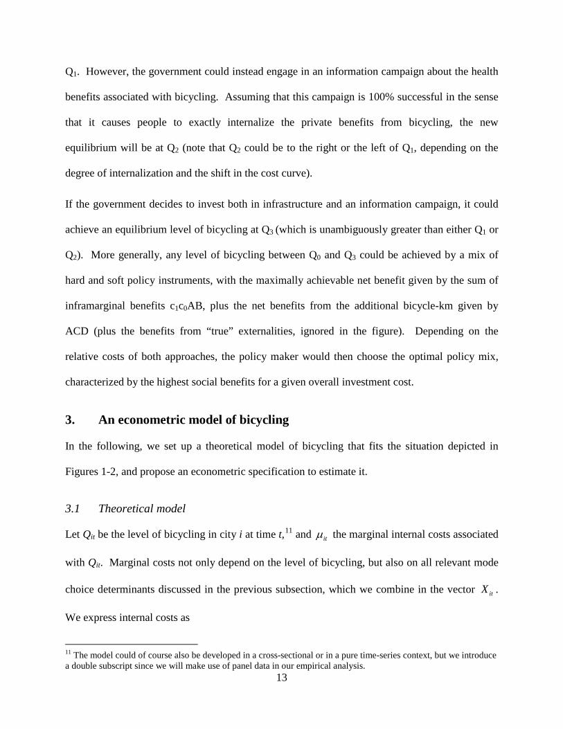
13

Q1. However, the government could instead engage in an information campaign about the health

benefits associated with bicycling. Assuming that this campaign is 100% successful in the sense

that it causes people to exactly internalize the private benefits from bicycling, the new

equilibrium will be at Q2 (note that Q2 could be to the right or the left of Q1, depending on the

degree of internalization and the shift in the cost curve).

If the government decides to invest both in infrastructure and an information campaign, it could

achieve an equilibrium level of bicycling at Q3 (which is unambiguously greater than either Q1 or

Q2). More generally, any level of bicycling between Q0 and Q3 could be achieved by a mix of

hard and soft policy instruments, with the maximally achievable net benefit given by the sum of

inframarginal benefits c1c0AB, plus the net benefits from the additional bicycle-km given by

ACD (plus the benefits from “true” externalities, ignored in the figure). Depending on the

relative costs of both approaches, the policy maker would then choose the optimal policy mix,

characterized by the highest social benefits for a given overall investment cost.

3. An econometric model of bicycling

In the following, we set up a theoretical model of bicycling that fits the situation depicted in

Figures 1-2, and propose an econometric specification to estimate it.

3.1 Theoretical model

Let Qit be the level of bicycling in city i at time t,11 and itµ the marginal internal costs associated

with Qit. Marginal costs not only depend on the level of bicycling, but also on all relevant mode

choice determinants discussed in the previous subsection, which we combine in the vector itX .

We express internal costs as

11 The model could of course also be developed in a cross-sectional or in a pure time-series context, but we introduce a double subscript since we will make use of panel data in our empirical analysis.

14

( , ) ( )it it it itf Q X g Xµ = + (1)

The function )(f ⋅ translates the level of bicycling into internal costs, with / 0itf Q∂ ∂ > , whereas

)( itg X controls for features that determine the level of bicycling (route, city and personal

characteristics). For a given level of bicycling Qit, the internal marginal cost of bicycling will be

lower in cities with better amenities for bicycling, all else equal. The translation between the

level of bicycling and associated internal costs may further depend on itX .

If consumers fully internalize internal benefits and do not consider externalities, they will equate

internal marginal costs with private marginal benefits:

,it p itMBµ = (2)

Making the assumption of full internalization allows us to substitute (2) into (1) and thus

eliminate internal marginal costs, which are unobservable. We could then quantify ,p itMB using

estimates for gross health benefits, specify a functional form for the functions (·)f and (·)g , and

estimate the corresponding parameters. However, this approach is not feasible if health benefit

estimates per km of bicycling do not significantly differ across observations.

If we are interested in assessing the degree of internalization of internal and external costs, we

need to estimate internal costs independently of internal benefits. Specifically, we express

internal costs as a function of observable variables combined in a vector itY :

( )it ith Yµ = (3)

15

The natural choice for itY are relevant mode determinants that the marginal bicyclist is likely

exposed to. To illustrate, suppose that kit itx X∈ refers to the hilliness of a city, expressed as

average elevation gain per trip from all modes combined. The corresponding instrument for

internal marginal costs itY would then be the average elevation gain from trips carried out by

bicyclists, or a distribution measure such as the 90th percentile.12 The underlying assumption of

this choice is that the elevation gain of the marginal bicyclists is higher if the average elevation

gain is higher, all else equal.13 An alternative would be to use psychological cost determinants

based on stated preferences as considered in Smith (1991), Rietveld and Daniel (2004) or Hunt

and Abraham (2007).

In addition to mode choice variables applied to bicyclists, itY can include measures of mode

substitution possibilities. For example, marginally increasing the level of bicycling in a city

where many short trips are carried out by car or public transportation should be associated with a

lower increment of internal costs, compared to increasing bicycling in a city where no such

“cheap” substitution possibilities exist.

There are two major empirical problems with estimating the marginal cost function: First,

internal costs are not observable, which requires the application of a latent variable framework if

we want to address the degree of internalization of internal and external benefits. Estimates from

latent variable approaches are indirect and therefore tend to be imprecise and sometimes also

12 In this one-dimensional example, the measure at the margin would be the maximum altitude (i.e. the steepest trip), however, since there are numerous factors determining the marginal cost at the same time the true exposure at the margin remains unknown. For practical reasons the mean or the 90th percentile can be used as proxies to reflect the distribution across cities of exposures at the margin. 13 Since h(Yit) is a multi-dimensional function, this assumption is somewhat stringent. For example, the marginal bicycle-km could take place in the rain on a crowded but completely flat road. One approach would be to create an index of marginal costs that depends on all known mode choice determinants, including personal characteristics of actual and potential riders, but such an index would have to rely on the same type of variables that we employ. We therefore chose the instrumental variable over the index approach.

16

sensitive to the model specification. Second and equally important, the data situation concerning

bicycling in general is poor. Our modeling framework therefore serves two main purposes: We

propose an empirical method to estimating the value of bicycle spending that is consistent with

economic theory, and we show what type of data would be required to make our approach more

policy-relevant.

3.2 A latent variable approach

Since the dependent variable has to be observable, we start by reverting (1):

( , ) ( )it it it itQ X Xψ µ κ= + (4)

with / 0itψ µ∂ ∂ > . The level of bicycling is a function of internal costs, with the effect possibly

being influenced by mode choice variables, and of mode choice variables themselves. A

linearized formulation of (4) is a model known as “Multiple Indicators and Multiple Causes”

(MIMIC) originally developed by Hauser and Goldberger (1971), as well as restricted versions.

We estimate the following system of equations:

( )·it it tt it i itiQ b X eb Xϕ λ µ β= + + ++ + (5)

it it itY uµ γ= + (6)

Comparing this system to the model (1)-(3) makes it clear that )( , ) / (it it ititf Q X Q Xϕ λ+= ,

( / )) (it it itg X X Xβ ϕ λ+= − , and ( )it ith Y Y γ= . The vectors of observed variables itX and itY

have dimensions (1 )x k and (1 )x m , respectively, with corresponding parameter vectors β and

λ of dimension ( 1)k x , and γ of dimension ( 1)m x .

17

Intuitively, we express the level of bicycling in city i at time t as a function of the internal costs

associated with an additional bicycle-km, while controlling for observable mode choice

characteristics collected in itX . These variables explain the “general” level of bicycling (e.g., we

expect a greater number of bicycle-km in a flat city than in a hilly one), whereas the latent

variable explains how “high up the marginal cost curve” bicycling takes place: If the level of

bicycling differs across two cities that are identical otherwise, marginally increasing bicycling is

associated with greater internal costs in the city where bicycle mode share is already higher. The

city- and time-specific constants bi and bt proxy for unobserved characteristics that influence the

level of bicycling. Unobserved characteristics that vary over both time and space end up in the

error term 2~ (0, )Qit Ne σ . The system can be estimated by maximum likelihood.

There are two natural restrictions that can be imposed on (5-6). First, the full MIMIC model

assumes that the proxy variables are measured imprecisely, which results in an additional error

term 2~ (0, )itu N µσ . This can improve precision of the estimate but also may be a cause for

unobserved variable bias. If instead no error is allowed, the MIMIC model reduces to the

“parametrically-weighted covariates” model (Yamaguchi, 2002).

Second, the marginal effect of a variable mit ity Y∈ on itQ (via itµ ) may vary over all or a subset

of mode choice characteristics:14

( )itm itm

it

Q Xy

γ ϕ λ⋅ +∂

=∂

(7)

14 Technically speaking, the effect is of course reversed: A high level of bicycling is associated with high marginal costs, not the other way around. We had to invert the relationship in order to estimate it.

18

The modulating effect itX λ has the interpretation of an interaction term. Consider the marginal

effect of ikit tx X∈ on the dependent variable:

itk k itk

it

Qx

β λ µ∂= + ⋅

∂ (8)

Variable kitx affects the dependent variable directly through kβ , but also indirectly via the latent

variable itµ . If the relationship between itµ on itQ is constant such that 0k kλ = ∀ , estimating

(5)-(6) is equivalent to the estimation of “Sheaf coefficients” (Heise, 1972).

3.3 Identification

In order to identify ,ϕ λ and γ , we have to set the origin, direction and unit of the latent

variable. The definition of the origin is implicit in (6), namely the exclusion of a constant in the

MC function, such that 0itµ = if all variables in itY are zero. This restriction is necessary

because an additional constant in the MC function could not be individually identified, because it

appears only as a product with other parameters.

The direction of the latent variable has to be specified because a positive itµ is equivalent to a

negative itµ , with the sign of ϕ and λ switched. The most natural way in our context is to

specify internal marginal costs to be positive.

The default to specify the unit of itµ is to set its standard deviation to 1, which is sufficient to

determine the relative size of areas a and d in Figure 1. The absolute magnitude of itµ is

required for policy decisions and can be derived from (2) by multiplying the parameter vector γ̂

19

by , ˆ/p it itMB µ . This is equivalent to assuming that cyclists fully internalize internal benefits, and

do not consider any external benefits.

If we are interested in the degree of internalization, we need to identify the unit of itµ

independent of internal benefits. For example, if internal (net) costs of bicycling another km

include money savings due to substituting away from driving or public transportation, we could

define the unit of itµ by setting the parameter on money savings mity to 1mγ = − (the sign must be

negative because these are internal benefits, i.e. negative costs). This yields an estimate of

internal marginal costs that is independent of ,p itMB . We can now estimate

,ˆit p it it itMB Eµ δ θ ε= + + (9)

where Eit refers to external benefits (computed outside the model, using techniques outlined in

Section 2.1), , [0,1]δ θ ∈ capture the extent to which internal and external benefits are

internalized, and itε is a random error. With fully informed and rational consumers, neoclassical

economic theory implies that 1δ = and 0θ = , which can be the basis of one-sided significance

tests against the alternative that cyclists do not fully internalize health effects 1δ < , and that they

internalize some of the external benefits ( 0θ > ). Again, this approach is not feasible if the

empirical estimates of internal benefits and externalities do not vary across observations.

3.4 The value of bicycle spending

We now turn to the computation of the areas in Figures 1 and 2. Area c has to be computed

outside of our model by specifically focusing on external effects of bicycling such as the share of

cost decreases in the health care system that accrues to non-riders, environmental benefits etc.

This is beyond the scope of this paper, and we will focus on the relative sizes of areas a, b and d.

20

To do this, we first estimate (5)-(6) subject to the identification restrictions outlined in the

previous subsection and use the parameter estimates to compute expected bicycle-km ˆitQ . We

then invert the relationship and express expected marginal costs as a function of expected

bicycle-km, observed explanatory variables and estimated parameters (detailed calculation in

appendix). The social value of bicycle spending in city i using our choice-based approach and

suppressing subscripts for convenience is15

00 2 2

Q QMC MC Q MCa b Q

∆ + ∆ ∆ ⋅∆+ = + (10)

where Q∆ is the difference in bicycle-km that results from the proposed policy, and 0MC∆ and

QMC∆ refer to the vertical difference between the old and new marginal cost function at 0Q =

and at 0Q , respectively. The difference between our approach and GHB is determined by the

relative sizes of areas a and d (derivation in appendix):

2 1 01 1 0 0

( )2 2

pQD a d Q Q MB Q α αα α −∆ ≡ − = ∆ ⋅ + − +

(11)

If the investment leads to a parallel shift of the MC curve such that 1 0α α= (which will be the

case if the mode determinants targeted by the policy are not modulator variables affecting the

relationship between internal cost and bicycle-km), the second term in (11) cancels. Taking

partial derivatives yields (derivation in Appendix)

15 Since a nonlinear function of a variable’s expectation is not the same as the expectation of a nonlinear function of the variable, we compute areas a, b and d for all city/year combinations and then take averages in our application.

21

00

20

11

0 ; 0 ;

( ) 0;2 ( )

pD DMC QQ MB

Q QD D cQα

∂ ∂= ∆ > = −∆ <

∂ ∂

∆ +∂ ∂= > = −

∂ ∂ ∆

(12)

In order, these results imply that the valuation of bicycle investments using our choice-based

approach, relative to that computed using GHB, 1.) increases with the bicycle mode share before

the investment (because this implies higher inframarginal benefits); 2.) decreases with the degree

of internalization of health benefits (because more costs are internalized and thus have to be

subtracted from benefits); 3.) increases with the slope of the new MC function (holding 0 ,Q Q∆

and pMB constant, a steeper MC function requires a larger downward shift, thus increasing

inframarginal benefits); and 4.) increases with the amount of additional bicycling if the new

intercept is negative, and vice versa (a higher Q∆ increases both a and d; the effect on the former

is larger if the “cheapest” bicycle-km are associated with negative costs).16

There is evidence implying that the relationship between bicycle spending and the resulting

increase in bicycling may be S-shaped, due to fixed costs and network effects (Levinson et al.,

2003). Combining this with an approximately linear valuation of bicycle-km that results from the

GHB approach (Lee and Skerrett, 2001) implies an S-shaped relationship between bicycle

spending and social benefits as well. Our approach affects this relationship, as it subtracts

internal costs from additional bicycle-km, but adds benefits to inframarginal km. At high levels

of bicycling, the latter term dominates and results in less flattening out of the spending/benefit

relationship relative to GHB, whereas the opposite occurs at low mode shares.

16 To provide some intuition on this last point, suppose that we shift the horizontal axis in Fig. 1 upwards. This decreases area d, while leaving area a unaffected.

22

Figure 3 illustrates, using the example of a parallel shift in the MC function. The upper right

quadrant shows the relationship between investment and bicycle-km. The upper left quadrant

translates bicycle-km to social value. This translation is approximately linear using the GHB

approach (solid line; we chose the units of social value per bicycle-km such that the slope is -1).

This leads to a relationship between spending and social value as shown by the solid line in the

lower left quadrant that is the mirror image of the spending/km relationship.

Figure 3: Spending, bicycle-km and social value

The relationship between bicycle-km and social value as computed by our approach is

represented by the dashed line. Compared to GHB, our approach leads to a lower social value

per additional bicycle-km at cycling levels below * / / 2pQ MB Qα= + ∆ (setting the first term in

eq. 11 to zero and solving for 0Q ), and higher above, meaning that the slope of the km/value

Spending($)

Spending ($)

Bicycle-km

Socialvalue

45°

*

2

pMB QQα

∆= +

S*

S**

**Q

Gross healthbenefits

Choice-based

Gross health benefits

Choice-based

45°

23

relationship is flatter below, and steeper above this threshold. At sufficiently high levels of

bicycling, the total social value from bicycling is higher when measured using our approach,

relative to GHB. In terms of the spending/social value relationship, our approach implies lower

social value per dollar of spending below S* than GHB and vice versa, leading to higher welfare

after an aggregate spending level of S**.

4. Application

In the following we describe our data and the employed variables, and present the results from an

empirical application of our model to eight Swiss cities.

4.1 Data

We use data from the Swiss national travel survey (Federal Statistical Office, 2007, 2012), a large

population based survey conducted approximately every five years. For methodological

comparability we restrict our analysis to data from the surveys from 1994, 2000, 2005 and 2010.

As part of the computer assisted telephone interview (CATI) subjects are asked to provide

information on one day of travel, tracking their mobility stage by stage. Travel mode, distance,

duration, trip purpose and additional variables are captured for each stage. Earlier surveys (1994

and 2000) captured start and endpoints of stages by address only, more recent surveys recorded

geo-coordinates using mapping software to assist CATI. Numerous additional variables are

available at the levels of trip, travel day (e.g. weather), subject (e.g. public transport pass or car

ownership), and household (e.g. number of vehicles available, including bikes).

We used Mapquest’s address search feature and GIS software to identify direct routes between

start and endpoints, which we overlaid with topographic data to derive elevation gains for each

trip stage. We extracted the number of fatal and severe accidents from annually published

accident statistics.

24

We compiled data for the 10 largest cities in Switzerland. We included all trips that originated or

ended within the limits of our sample cities. Because Lausanne and Lugano had very few

observed bicycle trips, we limited our analysis to Zurich, Bern, Basel, Geneva, St. Gallen,

Luzern, Biel and Winterthur, which gives us a total of 32 observations.

4.2 Variables

We use annual bicycle-km per capita as our dependent variable, which requires multiplying the

values from the Swiss Microcensus by 365. We work with annual rather than daily numbers

because the computation of health benefits presumes sustained long term behavior (see below).

Determinants of city-level cycling

As explanatory variables we use mode choice characteristics identified by the literature, and

which we can observe. For example, we do not have data on chosen routes and route

characteristics, which others have used successfully to identify important mode choice

determinants. (Dill and Gliebe, 2008; Menghini et al., 2009; Winters and Teschke, 2010) More

generally, we believe that the most important missing information is the extent and quality of the

bicycle network.

We control the observed level of bicycling using the following variables (for itX in eq. 5):

Hilliness: Average elevation gain of all trips (m/km). In hillier cities we expect fewer bicycle-

km per capita, all else equal.

City dispersion: Average distance of all trips. The relationship between city dispersion and

bicycle-km is nonlinear. Starting from low dispersion, increasing distances will presumably

lead to more bicycle-km, but when increasing dispersion further there will be a point where

very few trips are carried out by bicycle, thus reducing the number of bicycle-km.

25

Average precipitation: Number of days per year with >2 mm precipitation (Meteoswiss, 2012).

We expect less bicycling in rainy cities, all else equal.

Accident risk for bicyclists, computed as the number of accidents involving bicyclists that lead

to fatalities or severe injuries per million bicycle-km (source: Swiss Federal Roads Office,

ASTRA). We expect a higher bicycle mode share and therefore more bicycle-km in safer

cities, all else equal.

Price for public transportation (CHF per km) faced by the population as a whole, computed as

the price for a day pass within a city, divided by the average daily km travelled by public

transportation within the day pass zone, and adjusted for the fraction of the population that

have transportation passes.17 We accessed the price of day passes over time from the city

transportation offices of each city. Since bicycling and public transportation are substitutes at

least for short trips, we expect a positive relationship between this variable and bicycle-km.

Bicycle environment proxy: Survey responses from a large convenience sample of bicyclists

(N=5800 across our cities) to the statement “I like riding a bicycle in this city”. Available

answers ranged from 1 (completely disagree) to 6 (fully agree). (Pro Velo Switzerland, 2010)

Dummy for large cities, equal to one for Zurich, Basel, Bern and Geneva and zero otherwise.

These cities are more urban and have a more developed public transportation network

(including tramways) than the other cities in the sample.

Time dummies to identify the survey years 1994, 2000, 2005 and 2010 (reference category).

17 Because we are interested in the marginal rather than average cost, we set the marginal price per km of public transportation to zero for people with a transportation pass, and to 75% of the full price for people with “half-fare card” (the name comes from the fact that it reduces long-distance fares by 50%; however, the typical price for city-tickets is about 75% of the full price).

26

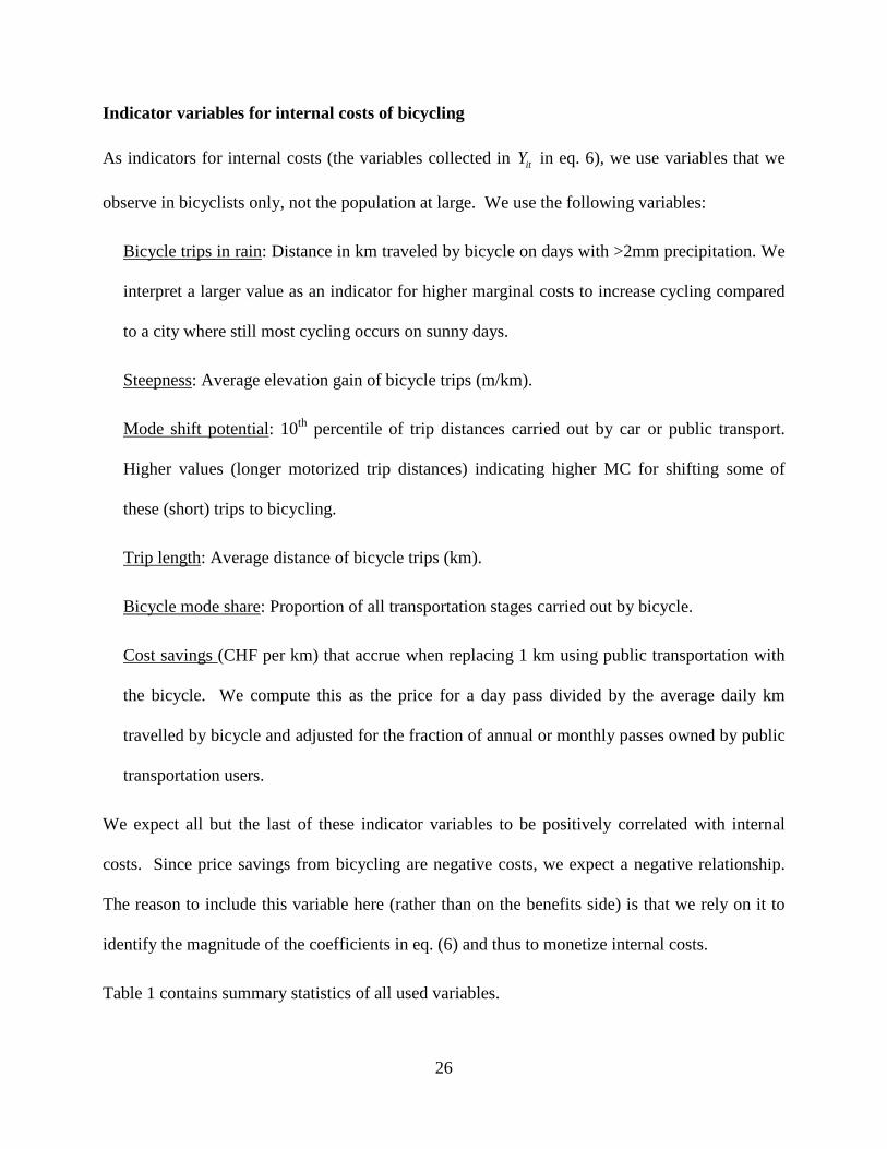
Indicator variables for internal costs of bicycling

As indicators for internal costs (the variables collected in itY in eq. 6), we use variables that we

observe in bicyclists only, not the population at large. We use the following variables:

Bicycle trips in rain: Distance in km traveled by bicycle on days with >2mm precipitation. We

interpret a larger value as an indicator for higher marginal costs to increase cycling compared

to a city where still most cycling occurs on sunny days.

Steepness: Average elevation gain of bicycle trips (m/km).

Mode shift potential: 10th percentile of trip distances carried out by car or public transport.

Higher values (longer motorized trip distances) indicating higher MC for shifting some of

these (short) trips to bicycling.

Trip length: Average distance of bicycle trips (km).

Bicycle mode share: Proportion of all transportation stages carried out by bicycle.

Cost savings (CHF per km) that accrue when replacing 1 km using public transportation with

the bicycle. We compute this as the price for a day pass divided by the average daily km

travelled by bicycle and adjusted for the fraction of annual or monthly passes owned by public

transportation users.

We expect all but the last of these indicator variables to be positively correlated with internal

costs. Since price savings from bicycling are negative costs, we expect a negative relationship.

The reason to include this variable here (rather than on the benefits side) is that we rely on it to

identify the magnitude of the coefficients in eq. (6) and thus to monetize internal costs.

Table 1 contains summary statistics of all used variables.

27

4.3 Computation of gross benefits

We calculate gross health benefits using the World Health Organisation’s Health Economic

Assessment Tool (HEAT) for cycling (Rutter et al., 2013; WHO, 2008). The tool uses a relative

risk estimate for all-cause mortality from a large Danish cohort study (Andersen et al., 2000) to

estimate avoided number of deaths from a certain level of observed cycling. We then monetize

the reduction in mortality using the value of a statistical life of $7.4 Mio (2006 dollars) used by

the US Environmental Protection Agency, which is equivalent to CHF 9.33 Mio (2010 francs).

We derive an average estimate for increasing the level of cycling by one km per capita per year in

our cities of CHF 0.50.

Table 1: Summary statistics Variable Unit Mean Std. Dev. Min Max (N=32) Av. bike-km km*year/cap 252.56 139.55 39.08 778.41 Hilliness (all modes) m/km 13.65 4.35 6.72 19.37 Dispersion (all modes) km 29.19 7.06 17.12 47.71 Rain days days/year 160.03 17.72 111.00 192.00 Accident risk fatal & severe acc.

per mio bike-km 0.72 0.39 0.12 1.54

Cost of public transport (all)

CHF/km 0.68 0.33 0.26 1.98

Subj. quality of bicycle environment

answers from 1 (very bad) to 6 (very good)

4.31 0.57 3.63 5.39

Large city 0/1 0.50 0.51 0 1 Bicycle-km in rain km 1.30 1.57 0 5.49 Elevation gain (bicycle) m/km 12.24 5.49 3.78 24.77 Mode shift potential (10th p. of car & PT trips)

km 0.93 0.13 0.71 1.22

Trip length (bicycle) km 3.92 1.56 1.93 10.67 Bicycle mode share % 6.43 2.82 1.59 11.53 Cost savings (switch from PT to bicycle)

CHF/km 0.34 0.14 0.15 0.61

28

4.4 Estimation

We estimate (5)-(6) by maximum likelihood in Stata, using code developed by Buis (2007).

Table 2 shows the estimation results. Model 1 is the most inclusive specification where we

included all mode choice determinants that seemed most important to us and for which we had

data, whereas Model 2 is a more restricted version where we removed some variables that were

statistically insignificant (dispersion and bicycle environment) and/or did not have the expected

sign (rain days). For each model, we estimated a “Sheaf coefficients” specification where 0λ =

in eq. (5) such that the relationship between internal costs and bicycle-km is constant and given

by ϕ (the models labeled 1a and 2a), as well as a version that allows the relationship between

bicycle-km and internal costs to vary over the “hilliness” variable (models 1b and 2b). We were

not able to further generalize this “parametrically-weighted covariates” model to the MIMIC

model with our data, because the estimation did not converge when an additional error term was

included.

The relationship between internal costs and bicycle-km is positive, consistent with our theory.

The coefficients on the variables that explain the city-level of bicycling (main equation) are quite

sensitive to the model specification. Among the variables that are significant in all specifications

are the “general” price for public transportation and the “large city” dummy, whereas accident

risk is only significant in the more restricted model 2. Hilliness is significant when it is also used

as a modulator variable, but not otherwise. Furthermore, the level of bicycling seems to be

increasing over time, as the time dummies are mostly negative (2010 is the reference category).

As for the indicator variables for internal costs, the amount of bicycling in rainy weather, the

distance of the most likely replacement trips and the bicycle mode share are positive and

statistically significant (although sometimes at p<0.1) in all models, whereas elevation gain

29

(“steepness”) and distance traveled by bicycle are significant only in some specifications. Price

savings from bicycling relative to using public transportation are always statistically significant

and negative, as expected. We re-scaled all coefficients in the MC equation such that the

coefficient on money savings per km is identically equal to minus one.18

Table 2: Regression results (dep. Variable: Bicycle-km per capita and year)

Model 1a Model 1b Model 2a Model 2b Coef p Coef p Coef p Coef p Main equation

Hilliness 12.34 0.361 -58.70 0.001 10.09 0.339 -33.28 0.015 Dispersion -5.19 0.260 -2.76 0.316

Raindays 1.76 0.514 4.27 0.025 Accident risk -119.51 0.191 -77.88 0.204 -175.40 0.021 -161.89 0.002

PTprice_all 247.93 0.032 214.23 0.001 215.05 0.021 158.44 0.011 bike_environment -59.52 0.540 -63.89 0.294

d_94 -92.44 0.220 -118.46 0.011 -61.83 0.325 -67.93 0.109 d_00 -88.33 0.205 -99.04 0.016 -81.74 0.221 -97.02 0.029 d_05 -47.75 0.524 11.17 0.825 -73.44 0.202 -61.56 0.115 Large 187.62 0.020 187.23 <0.001 160.65 0.020 145.14 0.001 Const. -677.03 0.217 -261.76 0.381 -449.41 0.088 110.47 0.383

lambda Const. (ϕ ) 446.032 0.001 2.248 0.551 340.838 <0.001 14.193 0.700

Hilliness ( 1λ )

28.953 <0.001

25.581 <0.001

MC equation Rain_bike 0.099 0.008 0.111 <0.001 0.116 0.003 0.113 <0.001

Steepness 0.007 0.703 0.017 0.112 0.005 0.829 0.007 0.523 Replace_trips 1.022 0.022 1.218 <0.001 0.978 0.066 1.104 0.001 Trip_length 0.059 0.203 0.056 0.025 0.056 0.268 0.042 0.097 Bike_mode 0.104 <0.001 0.126 <0.001 0.082 0.001 0.085 <0.001 PTprice_savings -1.000 0.018 -1.000 0.001 -1.000 0.053 -1.000 0.003

18 We report a t-statistic because we estimated the equation under the standard identification condition that the standard deviation of the constrained equation be one, which yields a regular estimate including standard errors for the cost savings variable. Scaling the point estimate and the associated standard error does not affect the t-statistic.

30

The sign on hilliness as a modulator variable may be counter-intuitive. We expected the

relationship between bicycling (the slope α of the MC function in Fig. 1) to be higher for hilly

cities. Since α is the inverse of the lambda function, a positive 1λ indicates a lower slope for

hilly cities. A possible explanation could be that in hilly cities, the general level of bicycling is

lower, such that a larger “reserve” of non-cyclists exists that could start to bicycle at relatively

low costs (recall that the coefficient on the indicator variable “steepness” is insignificant,

implying that this is not a major source of disutility in our sample).

Based on these parameter estimates we can now compute costs and benefits associated with an

increase in bicycling as discussed in Figures 1 and 2. Table 3 shows costs and benefits associated

with an increase in bicycling that would result from a public investment reducing accident risk by

25% (since accident risk is not a modulator variable, a decrease in accident risk implies a parallel

shift of the MC curve). These calculations are based on the parameter estimates from model 2b,

which is our preferred specification (the corresponding average numbers for the other models are

shown in Table A.1 in the appendix).

The increase in safety leads to an expected increase in average bicycling of about 29 km per

capita and year. Multiplied by the health benefits from a reduction in mortality as computed by

the HEAT tool (and the corresponding city populations), this yields an average benefit of CHF

1.9 mio using the GHB approach. This number corresponds to the sum of areas b and d in Fig. 1.

Using our choice-based approach and identifying internal costs by means of health benefits

computed by HEAT, we compute benefits that are less than half of those based on GHB (areas

a+b in Fig. 1). As shown in the theory section, this result depends on the baseline level of

bicycling. If we base the calculation on the minimum and maximum levels of bicycling in our

sample (corresponding to 39 resp. 778 km per year) rather than the mean, we obtain health

31

benefits of CHF 0.21 million and CHF 2.59 million, respectively. Increasing the baseline level of

bicycling increases the benefits computed with the choice-based approach relative to GHB,

because it leads to higher inframarginal benefits but has no effect on costs and benefits associated

with the additional bicycle-km.

Table 3: Costs and benefits of bicycling from reducing accident risk by 25%

Mean st.dev. HEAT benefits (CHF/km) 0.50 0.17

MB‘p (CHF/km) 1.63 0.34

∆Q (km/cap-year) 28.99 15.65

Baseline level of bicycling (km per cap. and year) Q0=253 Q0=39 Q0=778 Areas in Figs. 1 & 2 (mean values, mio CHF per city)

Fig. 1, area a 0.82 0.13 2.51

Fig. 1, area b 0.08 0.08 0.08

Fig. 1, area d 1.82 1.82 1.82

Fig. 2, area c0ACc1 2.66 0.41 8.21

Fig. 2, area ABC 0.28 0.28 0.28

Benefits (mean values, mio CHF per city & year) GHB based on HEAT 1.90 1.90 1.90

Choice-based, identification of MC through HEAT 0.89 0.21 2.59 Choice-based, identification of MC through cost savings 2.94 0.69 8.48

When identifying the magnitude of internal costs by means of cost savings from bicycling

relative to using public transportation, the implied benefits exceed those computed by HEAT.

Even though our results are generally sensitive to the model specification, this qualitative result

obtains in all models presented here.19 In order to map the resulting benefits to the areas marked

in Figure 2, we need to switch pMB′ and pMB . The benefits based on our approach are now area

c0ABc1, which is the sum of c0ACc1 (inframarginal benefits) and ABC (net benefits associated

19 In fact, we were not able to find an economically meaningful specification that yielded internalized benefits below those computed by HEAT.

32

with the additional bicycle-km), whereas the benefits based on HEAT are given by Q0A’B’Q1.

Not surprisingly, the former exceeds the latter, but this is not due to the method of benefits

computation per se (i.e. internal vs. external and inframarginal vs. marginal costs and benefits),

but because HEAT benefits are based on p pMB MB′< .

There are two explanations which can apply separately or jointly. First, it is possible that

consumers have altruistic preferences and internalize external benefits such as environmental

improvements (Eriksson and Forward, 2011) or a decrease in overall health costs. Second, total

internal benefits may exceed mortality-based benefits, which is the sole bases for the HEAT

numbers. If bicyclists also value decreased morbidity and generally improved physical fitness,

true internal health benefits may exceed CHF 0.5/km perhaps by enough to explain our results,

especially when considering the standard errors of our estimates.

Interestingly, the value of a statistical life (VSL) used for these computations is typically based

on mortality risk reductions only. As for internal benefits of bicycling, it is possible that people

value changes in risk-relevant parameters by more than only their impact on mortality. VSL

estimates based on hedonic wage regressions have been shown to be sensitive to the inclusion of

non-fatal risk (Black et al., 2003; Hintermann et al., 2010).20 Taking our results at face value and

making the neoclassical assumption of full internalization of internal benefits coupled with no

internalization of externalities, they would imply that the morbidity-adjusted value of risk is

about 3 times larger than that based solely on mortality.

Naturally, our capability to accurately model the complex relationships between determinants and

resulting bicycle behavior, given the limited quality of the underlying data, may serve as an

explanation. Since we are unable to control for some of the main determinants of bicycling (e.g. 20 While many hedonic wage studies include nonfatal risk in the regressions, its role is to control for wage-effects based on nonfatal risk. However, the VSL is computed solely based on the coefficient for fatal risk.

33

the quality and extent of a bicycle lane network for the main equation and route-specific

characteristics for the MC equation) we would like to emphasize that our results have to be

viewed with great caution and cannot be used to inform policy.

5. Conclusions

The proposed framework for valuation of bicycle investments adds an economic perspective to a

relatively young field of research, which to date has been studied primarily by health and

transport scientists. In particular, it expands the valuation beyond simple gross benefits

calculations, as provided by WHO’s popular HEAT tool and others. Our framework explicitly

considers internal costs to cyclists, thus allowing for the calculation of net benefits, which may

explain the often startling – and economically implausible – contrasts between large gross

benefits and surprisingly low levels of cycling. An optimal bicycle policy will maximize social

benefits. For a cost-benefit application of bicycle-related spending, the present value of annual

net benefits has to exceed the public investment.

By monetizing internal costs independently (i.e. via public transportation costs) from the benefits

(based on mortality reductions), the degree of internalization of benefits can be estimated (more

exactly, the net of internalizing internal benefits plus internalizing some externalities). This is

interesting in its own right, as it gives an indication about information costs and/or the presence

of altruistic preferences in bicyclists. Independent monetization further allows for

conceptualizing (quantifying) two key elements of a typical bicycle policies mix. The magnitude

of IMC indicates the extent to which predominantly “hard measures” – mainly infrastructure

improvements – are needed to lower internal costs. The degree of internalization on the other

hand indicates the potential of certain “soft measures” – educational campaigns that inform

people about the benefits of cycling and lead them to internalize these.

34

Finally, the framework considers inframarginal benefits, an improvement over traditional

approaches that ignore benefits to existing cycling/cyclists, even though the same measures

leading to new cycling often improve conditions for existing cycling too. Our analysis shows that

the higher the level of cycling is, the more relevant inframarginal benefits become. Our

framework is therefore preferable over gross benefits approaches in particular when valuing

investments over long assessment periods, which is appropriate given the often slow uptake of

usage, the long infrastructure lifetime and the significant non-linearities from network-effects.

A robust quantitative estimation of our framework is not yet possible, given the limited data

available to us, as well as others. The presented framework hence also serves as a rationale and

guidance for future investments in data collection efforts. While the travel survey data available

to us are quite rich and considered state of the art, they nonetheless are limited in their capability

to predict bicycle behavior. Based on existing literature and our expertise on the topic we identify

the main gaps in information relevant for internal costs at the level of routes, namely network

characteristics such as connectivity and route attributes such as objective and perceived safety

and infrastructure types. Besides richer data sets, progress in research on determinants of cycling

(including those with great spatial resolution), is needed to advance towards a quantitative

implementation of our framework.

35

Appendix

Computing slopes and intercepts in Fig. 1 using regression estimates

Estimating (5)-(6) and taking expectations gives

0ˆ ˆ ˆ ˆ ˆˆ ˆi t itit it itb bQ X X Yβ ϕ λ γ + + + + ⋅ = (A.1)

where we added a zero-subscript to indicate the benchmark (i.e. pre-investment) situation.

Substituting ˆit itMC Y γ= and inverting (A.1) leads to

0 0 0 0ˆˆˆit it it itMC c Qα= + (A.2)

with 01

ˆˆˆ t

ti

iXϕα

λ+= (A.2)

0 0ˆ( )ˆˆˆˆ it i tit itc b Xb βα− + += (A.3)

Suppose that bicycle spending shifts the marginal cost function by changing the mode choice

determinant kit itx X∈ (for example accident risk). The new MC function becomes

1 1 1 1ˆˆˆit it it itMC c Qα= + (A.5)

with 11ˆ ˆˆ

ˆ it kit it kX x

αλ λϕ

=+ + ∆

(A.6)

1 1ˆ ˆˆ ( ˆˆ ˆ )it

kit it it ki tb bc X xα β β− + += + ∆ (A.7)

( )1 0ˆ ˆ ˆ ˆ ˆk

it it it k k itQ Q x β λ µ= + ∆ + (A.8)

If kitx is not a modulator variable such that 0kλ = , the slope will remain unchanged at 0ˆ itα ,

whereas the intercept is adjusted by 0ˆ ˆi tt

ki kx βα− ∆ .

36

Derivation of equations (11) and (12)

Suppressing subscripts and setting pMC MB= , the areas in Figure 1 are given by

( )0 0

( ) / 2

· ( ) / 2

· / 2

Q

p Q

Q

b MC Q

d Q MB MC Q

a Q MC MC

= ∆ ∆

= ∆ − ∆

∆ + ∆

⋅

∆

=

⋅ (A.9)

with 1 0Q Q Q∆ = − . If consumers internalize private health benefits only partially, or if they

internalize some of the external benefits, pMB is replaced by pMB′ in Fig. 2, but all else remains

the same. We now subtract a from d while making the following substitutions:

0 0 1

0 0 1 1

0 1 0 1

( )

( )p p

MC c cMB Q MB QQ Q

α α

α α α

∆ = −= − − −

= − + ∆

(A.10)

0 0 0 1 1 0

0 1 0 1 0

1

( )

( )QMC c Q c Q

c c QQ

α α

α αα

∆ = + − +

= − − −= ∆

(A.11)

Using these substitutions, we get

20 1 0 1

0 1

2 2 1 01 1 0 0

( ) 2 ( )2 2

( )2 2

p

p

Q Q QD a d Q Q MB

QQ Q MB Q

α α α α

α αα α

− + ∆ ∆≡ − = −∆ ⋅ +

−∆ = ∆ ⋅ + − +

(11)

37

The partial derivatives of (10) w.r.t. 0,pMB α and 1α are straightforward. Using (A.2) and

(A.10), the partial w.r.t. 0Q and Q∆ are

1 0 1 00

1 1 0 0 1 0

0 1 0

( )

( ) ( )

( )p p

D Q QQ

Q Q MB c MB cc c MC

α α α

α α

∂= ∆ + −

∂= − = − − −

= − = ∆

1 1 0

1 1 1

( ) p

p

D Q Q MBQ

Q MB c

α α

α

∂= ∆ + −

∂ ∆= ⋅ − = −

Table A.1: Benefits from reducing accident risk by 25%, all models

Model 1a Model 1b Model 2a Model 2b

Mean St.de

v Mea

n St.de

v Mean St.dev Mean St.dev Parameters

HEAT benefits (CHF/km) 0.503 0.168

0.503 0.168 0.503 0.168 0.503 0.168

MB’p

(CHF/km) 1.722 0.369 2.16

7 0.424 1.518 0.335 1.633 0.341

∆Q (km/cap-year) 0.930 0.502

0.494 0.267

31.407

16.961

28.987

15.654

Benefits from reducing acc. risk by 25% (mio CHF per city and year)

GHB based on HEAT (areas b+d in Fig. 1) 0.061 0.050

0.032 0.027 2.057 1.703 1.899 1.572

Choice-based, MC identified through HEAT (areas a+b in Fig. 1) 0.017 0.013

0.010 0.009 0.922 0.665 0.894 0.807

Choice-based, MC identified through cost savings (area c0ABc1 in Fig. 2) 0.060 0.051

0.042 0.037 2.916 2.293 2.939 2.545

38

Literature

Ainsworth, B.E., Haskell, W.L., Whitt, M.C., Irwin, M.L., Swartz, A.M., Strath, S.J., O'Brien, W.L., Bassett, D.R., Jr., Schmitz, K.H., Emplaincourt, P.O., Jacobs, D.R., Jr., Leon, A.S., 2000. Compendium of physical activities: an update of activity codes and MET intensities. Med Sci Sports Exerc 32, S498-504.

Allen-Munley, C., Daniel, J., Dhar, S., 2004. Logistic model for rating urban bicycle route safety. Pedestrians and Bicycles; Developing Countries, 107-115.

Andersen, L.B., Schnohr, P., Schroll, M., Hein, H.O., 2000. All-cause mortality associated with physical activity during leisure time, work, sports, and cycling to work. Arch Intern Med 160, 1621-1628.

Benabou, R., Tirole, J., 2006. Incentives and Prosocial Behavior. American Economic Review 96, 27.

Bernheim, B.D., Rangel, A., 2007. Behavioral public economics: Welfare and policy analysis with nonstandard decision-makers, in: Diamond, P. (Ed.), Behavioral economics and its applications. Princeton University Press, Princeton, p. 312.

Berrigan, D., Pickle, L.W., Dill, J., 2010. Associations between street connectivity and active transportation. Int J Health Geogr 9, 20.

Black, D.A., Galdo, J., Liqun, L., 2003. How Robust are Hedonic Wage Estimates of the Price of Risk. National Center for Environmental Economics

Syracuse University, Washington, D.C., p. 104. Buehler, R., Pucher, J., 2012. Cycling to work in 90 large American cities: new evidence on the

role of bike paths and lanes. Transportation 39, 409-432. Buis, M.L., 2007. PROPCNSREG: Stata program fitting a linear regression with a proportionality

constraint by maximum likelihood. Caulfield, B., Brick, E., McCarthy, O.T., 2012. Determining Bicycle Infrastructure Preferences--

A Case Study of Dublin. Transportation Research: Part D: Transport and Environment 17, 413-417.

Cavill, N., Kahlmeier, S., Rutter, H., Racioppi, F., Oja, P., 2009. Economic Analyses of Transport Infrastructure and Policies Including Health Effects Related to Cycling and Walking: A systematic review. Transport Policy 15, 291-304.

de Geus, B., De Bourdeaudhuij, I., Jannes, C., Meeusen, R., 2008. Psychosocial and environmental factors associated with cycling for transport among a working population. Health Educ Res 23, 697-708.

de Hartog, J.J., Boogaard, H., Nijland, H., Hoek, G., 2010. Do The Health Benefits Of Cycling Outweigh The Risks? Environ Health Perspect.

de Nazelle, A., Nieuwenhuijsen, M.J., Anto, J.M., Brauer, M., Briggs, D., Braun-Fahrlander, C., Cavill, N., Cooper, A.R., Desqueyroux, H., Fruin, S., Hoek, G., Panis, L.I., Janssen, N., Jerrett, M., Joffe, M., Andersen, Z.J., van Kempen, E., Kingham, S., Kubesch, N., Leyden, K.M., Marshall, J.D., Matamala, J., Mellios, G., Mendez, M., Nassif, H., Ogilvie, D., Peiro, R., Perez, K., Rabl, A., Ragettli, M., Rodriguez, D., Rojas, D., Ruiz, P., Sallis, J.F., Terwoert, J., Toussaint, J.F., Tuomisto, J., Zuurbier, M., Lebret, E., 2011. Improving health through policies that promote active travel: A review of evidence to support integrated health impact assessment. Environ Int. 37, 766-777.

Dill, J., 2009. Bicycling for Transportation and Health: The Role of Infrastructure. Journal of Public Health Policy 30, S95-S110.

39

Dill, J., Gliebe, J., 2008. Understanding and Measuring Bicycling Behavior: a Focus on Travel Time and Route Choice. Oregon Transportation Research and Education Consortium (OTREC), Portland, OR, p. 70.

Dumbaugh, E., 2005. Safe Streets, Livable Streets. Journal of the American Planning Association 71, 283-300.

Ellison, R.B., Greaves, S.P., 2011. Travel time competitiveness of cycling in Sydney. Elston, M.A., 2002. Commentary: Attitudes to women's bicycling have changed. Brit Med J 325,

139-139. Eriksson, L., Forward, S.E., 2011. Is the Intention to Travel in a Pro-environmental Manner and

the Intention to Use the Car Determined by Different Factors? Transportation Research: Part D: Transport and Environment 16, 372-376.

Federal Statistical Office, 2007. Mobilität in der Schweiz: Ergebnisse des Mikrozensus 2005 zum Verkehrsverhalten. BfS, ARE, Neuchâtel, pp. 38, 41.

Federal Statistical Office, 2012. Mobilität in der Schweiz: Ergebnisse des Mikrozensus Mobilität und Verkehr 2010. BfS, ARE, Neuchâtel.

Gotschi, T., 2011. Costs and Benefits of Bicycling Investments in Portland, Oregon. Journal of Physical Activity and Health 8, S49-S58.

Harris, M.A., Reynolds, C.C., Winters, M., Chipman, M., Cripton, P.A., Cusimano, M.D., Teschke, K., 2011. The Bicyclists' Injuries and the Cycling Environment study: a protocol to tackle methodological issues facing studies of bicycling safety. BMJ Publishing Group.

Hauser, R.M., Goldberger, A.S., 1971. The Treatment of Unobservable Variables in Path Analysis. Sociological Methodology 3, 37.

Heinen, E., Handy, S., 2012. Similarities in Attitudes and Norms and the Effect on Bicycle Commuting: Evidence from the Bicycle Cities Davis and Delft. Int. J. Sustain. Transp. 6, pp 257-281.

Heise, D.R., 1972. Employing nominal variables, induced variables, and block variables in path analysis. Sociological Methods & Research 1, 27.

Hintermann, B., Alberini, A., Markandya, A., 2010. Estimating the value of life using labor market data: Are the results trustworthy? . Applied Economics 42, 1085-1100.

Hunt, J.D., Abraham, J.E., 2007. Influences on Bicycle Use. Transportation 34, 453-470. Int Panis, L., de Geus, B., Vandenbulcke, G., Willems, H., Degraeuwe, B., Bleux, N., Mishra, V.,

Thomas, I., Meeusen, R., 2010. Exposure to particulate matter in traffic: A comparison of cyclists and car passengers. Atmospheric Environment 44, 2263-2270.

Kirner Providelo, J., Sanches, S.d.P., 2011. Roadway and Traffic Characteristics for Bicycling. Transportation 38, 765-777.

Krizek, K., Forsyth, A., Baum, L., 2009. Walking and Cycling International Literature Review. Department of Transport - Walking and Cycling Branch, Melbourne, Australia.

Krizek, K., Poindexter, G., Barnes, G., Mogush, P., 2007. Analysing the Benefits and Costs of Bicycle Facilities via Online Guidelines. Planning, Practice & Research 22, 197-213.

Lee, I.M., Skerrett, P.J., 2001. Physical activity and all-cause mortality: what is the dose-response relation? Med Sci Sports Exerc 33, S459-471; discussion S493-454.

Levinson, D., Karamalaputi, R., Chen, W., 2003. If They Come, Will You Build It? Urban Transportation Growth Models. Department of Civil Engineering, University of Minnesota, St.Paul, p. 73.

Litman, T., 2004. Quantifying the Benefits of Nonmotorized Transportation For Achieving Mobility Management Objectives. Transportation Research Record 1441, 134-140.

40

Lusk, A.C., Furth, P.G., Morency, P., Miranda-Moreno, L.F., Willett, W.C., Dennerlein, J.T., 2011. Risk of injury for bicycling on cycle tracks versus in the street. Injury Prevention 17, 131-135.

Menghini, G., Carrasco, N., Schussler, N., Axhausen, K.W., 2009. Route Choice of Cyclists: discrete choice modelling based on GPS-data, Arbeitsberichte Verkehrs- und Raumplanung. IVT, ETH Zurich, Zurich.

Meteoswiss, 2012. "Langjährige homogene Temperatur- und Niederschlagsreihen der Schweiz". http://www.meteoswiss.admin.ch/web/en/services/data_portal.html.

Parkin, J., Wardman, M., Page, M., 2008. Estimation of the Determinants of Bicycle Mode Share for the Journey to Work Using Census Data. Transportation 35, 93-109.

Plaut, P.O., 2005. Non-motorized Commuting in the US. Transportation Research: Part D: Transport and Environment 10, 347-356.

Pro Velo Switzerland, 2010. "Velostaedte" Survey. www.velostaedte.ch. Release date: May 20th, 2010

Pucher, J., Dill, J., Handy, S., 2010. Infrastructure, programs, and policies to increase bicycling: An international review. Preventive Medicine 50, S106-S125.

Rietveld, P., Daniel, V., 2004. Determinants of Bicycle Use: Do Municipal Policies Matter? Transportation Research: Part A: Policy and Practice 38, 531-550.

Rojas-Rueda, D., de Nazelle, A., Tainio, M., Nieuwenhuijsen, M.J., 2011. The health risks and benefits of cycling in urban environments compared with car use: health impact assessment study. BMJ: British Medical Journal 343.

Rutter, H., Cavill, N., Racioppi, F., Dinsdale, H., Oja, P., Kahlmeier, S., 2013. Economic Impact of Reduced Mortality Due to Increased Cycling. Am J Prev Med 44, 89-92.

Saelensminde, K., 2004. Cost-Benefit Analyses of Walking and Cycling Track Networks Taking into Account Insecurity, Health Effects and External Costs of Motorized Traffic. Transportation Research: Part A: Policy and Practice 38, 593-606.

Sener, I.N., Eluru, N., Bhat, C.R., 2009. An Analysis of Bicycle Route Choice Preferences in Texas, US. Transportation 36, 511-539.

Smith, B.H., 1991. Anxiety as a Cost of Commuting to Work. Journal of Urban Economics 29, 260-266.

Thakuriah, P., Metaxatos, P., Lin, J., Jensen, E., 2012. An Examination of Factors Affecting Propensities to Use Bicycle and Pedestrian Facilities in Suburban Locations. Transportation Research: Part D: Transport and Environment 17, 341-348.

Troped, P.J., Saunders, R.P., Pate, R.R., Reininger, B., Ureda, J.R., Thompson, S.J., 2001. Associations between self-reported and objective physical environmental factors and use of a community rail-trail. Prev Med 32, 191-200.

Vandenbulcke, G., 2011. Cycle Commuting in Belgium: Spatial Determinants and 'Re-Cycling' Strategies. Transportation Research: Part A: Policy and Practice 45, 118-137.

Wang, G., Macera, C.A., Scudder-Soucie, B., Schmid, T., Pratt, M., Buchner, D., 2005. A Cost-Benefit Analysis of Physical Activity Using Bike/Pedestrian Trails. Health Promot Pract 6, 174-179.

Wardman, M., Tight, M., Page, M., 2007. Factors Influencing the Propensity to Cycle to Work. Transportation Research: Part A: Policy and Practice 41, 339-350.

WHO, 2008. Health Economic Assessment Tool for cycling. World Health Organization Office for Europe.

41

Winters, M., Teschke, K., 2010. Route Preferences Among Adults in the Near Market for Bicycling: Findings of the Cycling in Cities Study. American Journal of Health Promotion 25, 40-47.

Woodcock, J., Edwards, P., Tonne, C., Armstrong, B.G., Ashiru, O., Banister, D., Beevers, S., Chalabi, Z., Chowdhury, Z., Cohen, A., Franco, O.H., Haines, A., Hickman, R., Lindsay, G., Mittal, I., Mohan, D., Tiwari, G., Woodward, A., Roberts, I., 2009. Public health benefits of strategies to reduce greenhouse-gas emissions: urban land transport. Lancet 374, 1930-1943.

Xing, Y., Handy, S.L., Mokhtarian, P.L., 2010. Factors associated with proportions and miles of bicycling for transportation and recreation in six small US cities. Transport Res D-Tr E 15, 73-81.

Yamaguchi, K., 2002. Regression models with parametrically weighted explanatory variables. Sociological Methodology 2002, Vol 32 32, 219-245.