Valuation of Financial Instruments: Theoretical Overview ... · 1/18 Valuation of Financial Instruments: Theoretical Overview with Applications in Bloomberg Introduction In practice,

1/18

Valuation of Financial Instruments: Theoretical Overview with Applications in Bloomberg

Introduction

In practice, company valuation deals with the valuation of stocks, bonds and other financial instruments issued by the company of interest. In this chapter, we take an overview of valuation techniques in accordance with different types of securities. The understanding of differences between financial instruments is crucial for the valuation process, where valuation methods differ for types of securities.

A financial instrument is a tradable asset of any kind; either cash, evidence of an

ownership interest in an entity, or a contractual right to receive or deliver cash or another financial instrument. Valuation of certain financial instruments helps to determine the value of the whole company or just its part. It might seem that valuation of financial instruments is mostly important for financial firms, since securities issuing and trading is the biggest part of their business, but it becoming more important for production and service companies as well. Non-financial companies are actively participating in the bond market and placing free cash in cash and derivative instruments.

Boards, management and investors require valuations of equity and debt instruments for

numerous purposes including planning and reporting requirements associated with: audit compliance, corporate and personnel tax, deferred compensation, employee stock ownership plan formation and reporting, fundraises/recapitalizations, mergers, acquisitions and divestitures, litigation support, and transaction advisory services including fairness and solvency opinions.

Equity, stock, options, and derivative valuations depend on a number of variables. How

was the price of the underlying enterprise determined? How will pricing and value be determined going forward? These analyses often require complex formulas and key data/assumptions that unfortunately can lead to controversy or dispute. These analyses are the subjects of discussion in this chapter.

To address the practical side of valuation process, we provide our overview with examples

and tasks in Bloomberg Terminal, which is currently one of the most popular electronic analytical and trading platforms worldwide. For valuation purposes, Bloomberg provides investors and traders with all of the necessary tools for basic valuation of financial instruments. We believe that these examples will help students to understand how valuation works in real life and give an experience of using Bloomberg Terminal for future job opportunities.

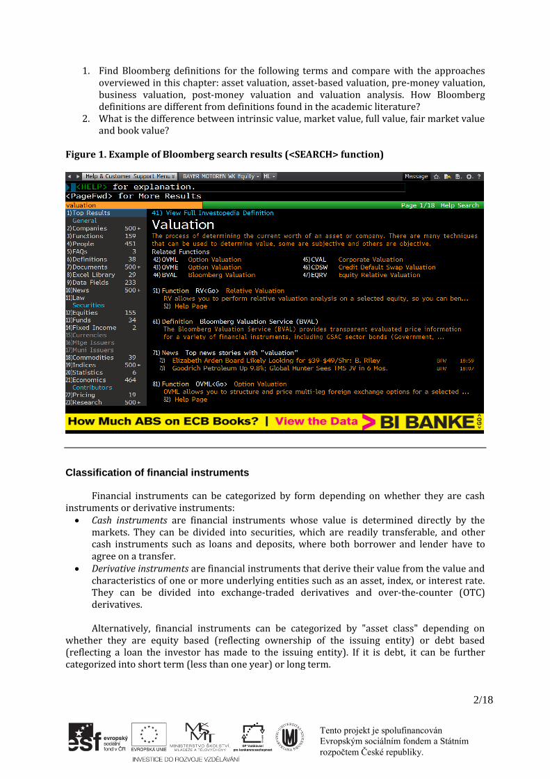
Example 1. Basic financial definitions in Bloomberg

Bloomberg Terminal offers brief, but comprehensive definitions of core valuation concepts. For example, valuation defined as the process of determining the current worth of an asset or company.

Tento projekt je spolufinancován

Evropským sociálním fondem a Státním

rozpočtem České republiky.

2/18

1. Find Bloomberg definitions for the following terms and compare with the approaches overviewed in this chapter: asset valuation, asset-based valuation, pre-money valuation, business valuation, post-money valuation and valuation analysis. How Bloomberg definitions are different from definitions found in the academic literature?

2. What is the difference between intrinsic value, market value, full value, fair market value and book value?

Figure 1. Example of Bloomberg search results (<SEARCH> function)

Classification of financial instruments

Financial instruments can be categorized by form depending on whether they are cash instruments or derivative instruments: Cash instruments are financial instruments whose value is determined directly by the

markets. They can be divided into securities, which are readily transferable, and other cash instruments such as loans and deposits, where both borrower and lender have to agree on a transfer.

Derivative instruments are financial instruments that derive their value from the value and characteristics of one or more underlying entities such as an asset, index, or interest rate. They can be divided into exchange-traded derivatives and over-the-counter (OTC) derivatives. Alternatively, financial instruments can be categorized by "asset class" depending on

whether they are equity based (reflecting ownership of the issuing entity) or debt based (reflecting a loan the investor has made to the issuing entity). If it is debt, it can be further categorized into short term (less than one year) or long term.




3/18

Table 1. Financial instruments classification according to their asset group and traded market

Asset class Instrument type

Securities Other cash Exchange-traded

derivatives OTC derivatives

Equity Stocks - Stock options, equity futures

Stock options, exotic instruments

Long-term debt Bonds Loans Bond futures Interest rate swaps

and options

Short-term debt Bills, commercial

papers

Deposits, certificates of deposit

Interest rate futures

Forward rate arguments

Foreign Exchange - FX spot Currency futures FX options and

swaps

Example 2. Financial instruments classification in Bloomberg

Bloomberg classification of financial instruments is more straightforward. There are eleven basic financial instrument classes in Bloomberg (main menu):

1. Sovereign (government) bonds 2. Credit (corporate) bonds 3. Mortgages 4. Money markets instruments 5. Municipal bonds 6. Preferred instruments 7. Equities (include stocks, ETFs, warrants, equity futures, equity options, index

options, etc.) 8. Commodities 9. Indices 10. Currencies 11. Derivatives and structured notes

Why such classification is utilized in Bloomberg? What approaches to instrument

classification is used in Bloomberg?

Valuing stocks

The problem in valuation of stocks is that there are relatively overwhelming number of valuation techniques found in the literature and employed by analysts. Generally speaking, there is no one method which is best suited for every situation. In practice, the decision on stock purchase is usually based on the combination of several valuation approaches and overall analysis of the firm. These approaches often make very different assumptions about fundamentals but they share some common characteristics allowing their classification. Classification makes it easier to understand where individual valuation models fit into the big picture, why they provide different results and when they fundamental errors in logic.

In the broadest possible terms, stock valuation methods fall into two main categories:

absolute and relative valuation approaches. Absolute valuation attempts to find an intrinsic value of the stock based on company's fundamentals, such as dividends, cash flow and growth rate. Valuation models that fall into this category include the dividend discount model, discounted cash flow model, residual income models and asset-based models. In contrast to absolute valuation models, relative valuation models operate by comparing the company in question to other similar companies. These methods generally involve calculating multiples or ratios,




4/18

such as the price-to-earnings ratio, earnings-per-share ratio, price-to-book value ratio, prices-to-sales ratio, and comparing them to the multiples of other comparable firms. There is one additional approach for stock valuation called contingent claim valuation, which uses option pricing models and in our survey falls under the rubric of real option valuation.

Within each of valuation approaches lay a myriad of sub-approaches, which share

common characteristics while varying on details. Absolute valuation models can take three forms – dividend based valuation, cash flow based valuation and residual income valuation. Relative valuation models can be structured around different multiples (earnings, book value and revenues) and an asset can be compared to very similar companies, the sector or even against the entire market.

Example 3. Financial Instrument Search

Use Security Finder to get a list of most popular common stocks available for trading in Bloomberg. According to what criteria the list is compiled?

Figure 2. Example of Bloomberg Security Finder results (<SECF> function)

Absolute Valuation Techniques

Beginning with John Burr Williams' PhD thesis “The Theory of Investment Value” in 1938, analysts have developed this insight into a group of valuation models known as discounted cash flow (DCF) valuation models. DCF models—which view the intrinsic value of common stock as the present value of its expected future cash flows—are a fundamental tool in both investment management and investment research. The value of an asset must be related to the benefits or returns we expect to receive from holding it. The concept that an asset’s value is the present value of its (expected) future cash flows in its simplest form is usually expressed by the following equation:




5/18

𝑉0 = ∑𝐶𝐹𝑡

(1 + 𝑟)𝑡

𝑛

𝑡=1

,

where 𝑉0 is the value of the asset at time t=0 (today), n is the number of cash flow periods considered, 𝐶𝐹𝑡 is the cash flow (or the expected cash flow, for risky cash flows) at time t and r is the discount rate or required rate of return.

Example 4. Stock description and basic information

Let use IBM stock as an example for our valuation exercises. What are the business activities of the company?

Figure 3. Bloomberg screen for company description (<DES> function)

Figure 3 provides basic information about the company stock. What is the company

current price (at 16:01) and if you have the budget of 10.000 USD how many stocks you can buy? What is the company market capitalization and how many shares have been issued, respectively, what is the number of shares outstanding and what is the one year maximum and minimum? How is measured the sensitivity of the stock to the market and what is actual value of this sensitivity?

Several basic DCF models should be considered a cornerstone of absolute stock valuation

according to the used notion of returns (dividends, free cash flow and residual income):

The dividend discount model (DDM) defines cash flows as dividends, which are the only form of cash returns for an investor who buys and holds a share of stock. It should be noted that dividends are less volatile than earnings and other return concepts, thus making DDM values less sensitive to short-run fluctuations in underlying value than




6/18

alternative DCF models. Analysts often view DDM values as reflecting long-run intrinsic value. However, DDM models cannot not be applied to every public company, for the reason that not every stock pays dividends. Additionally, analysts should pay attention to broad trends in dividend policy, since dividend policy practices have international differences and change through time, even in one market1. The DDM is the simplest and oldest present value approach to valuing stock.

Free cash flow to the firm (FCFF) is cash flow from operations minus capital expenditures (reinvestment in new assets, including working capital, which are needed to maintain the company as a going concern). FCFF is the part of the cash flow generated by the company’s operations that can be withdrawn by bondholders and stockholders without economically impairing the company. Free cash flow to equity (FCFE) is cash flow from operations minus capital expenditures, from which we net all payments to debt holders. FCFF is a pre-debt free cash flow concept; FCFE is a post-debt free cash flow concept. The FCFE model is the baseline free cash flow valuation model for equity, but the FCFF model may be easier to apply in several cases, such as when the company’s leverage (debt in its capital structure) is expected to change significantly over time. Free cash flow (FCFF or FCFE) can be calculated for any company.

Residual income for a given time period is the earnings for that period in excess of the

investors’ required return on beginning-of-period investment (common stockholders’ equity). The required rate of return is investors’ opportunity cost for investing in the stock: the highest expected return available from other equally risky investments, which is the return that investors forgo when investing in the stock. The residual income model states that a stock’s value is book value per share plus the present value of expected future residual earnings. Several popular valuation techniques, such as Economic Value Added developed by consulting firm Stern Stewart & Co., are based on residual income concept.

To use the DDM in the indefinite time, expected dividends should be forecasted, usually in

simplified, not individual company-specific manner. Future dividends can be forecast by assigning the stream of future dividends to one of several stylized growth patterns: constant growth forever (the Gordon growth model), two distinct stages of growth (the two-stage growth model and the H-model) or three distinct stages of growth (the three-stage growth model). The Gordon growth model, developed by Gordon and Shapiro (1956) and Gordon (1962), assumes that dividends grow indefinitely at a constant rate: 𝐷𝑡 = 𝐷𝑡−1(1 + 𝑔), where 𝐷𝑡 is the expected dividend payable at time t and g is the expected constant growth in dividends (usually measured by the growth in GDP, as he market’s implied growth rate for a stock or derived from company fundamentals2). This assumption, applied to general DCF model, yields a geometric series, which can be simplified as:

𝑉0 =𝐷0(1 + 𝑔)

𝑟 − 𝑔 or 𝑉0 =

𝐷1

𝑟 − 𝑔.

The strongest critic of the Gordon growth model lies in its oversimplification about stable

dividend growth rate from now into the indefinite future, making the model unrealistic for many or even most companies (especially in periods of economic and financial crises). For many publicly traded companies, practitioners assume growth falls into three stages (see Sharpe, Alexander, and Bailey 1999): growth phase (rapidly expanding markets, high profit margins, and an abnormally high growth rate in earnings per share), transition phase (growth slows as competition puts pressure on prices and profit margin or because of market saturation) and

1 Lesser amount of US companies have paid dividends than European comparable companies (CITATION IS

NEEDED) 2 The sustainable growth rate depends on the ROE and, using the DuPont analysis, can be expanded further to

include various ratios used in fundamental analysis.




7/18

mature phase (fundamentals stabilize at levels that can be sustained long term). The growth-phase concept provides the intuition for multistage discounted cash flow (DCF) models of all types, including multistage dividend discount models. Two-stage dividend discount model provides a useful example:

𝑉0 = ∑𝐷0(1 + 𝑔𝑆)𝑡

(1 + 𝑟)𝑡+

𝐷0(1 + 𝑔𝑆)𝑛(1 + 𝑔𝐿)

(1 + 𝑟)𝑛(𝑟 − 𝑔𝐿)

𝑛

𝑡=1

,

where 𝑔𝑆 is an extraordinary short-term rate and 𝑔𝐿 is a normal long-term rate (usually matches with the growth rate of the Gordon growth model). The two-stage model might be transformed into H-model to account for linear decline from initial supernormal growth to a normal rate at the end (see Fuller and Hsia, 1984). Various versions of the three-stage DDM depict all three stages of growth and usually customized by analyst and might be enlarged to depict any variety of growth patterns (multiple stages).

Example 5. Bloomberg dividend discount model

Dividend discount model is one of the basic valuation functions in Bloomberg, providing automatic calculations for stages of growth, interest rates, risk premiums and growth rate. Selection of growth patterns at different stages is easily customized by the analyst. Figure 4. Results of dividend discount model computations in Bloomberg (<DDM> function)

What type of dividend discount model is utilized in Bloomberg? What kind of bond is used

for automatic calculation of bond rate? What index is used for calculation of beta? How will theoretical price change, if we change the number of growth years, transitional years and growth rate at maturity?




8/18

The value of equity or whole firm can also be found by discounting FCFE or FCFF at the

required rate of return on equity r3:

𝑉0 = ∑𝐹𝐶𝐹𝐸𝑡

(1 + 𝑟)𝑡 or 𝑉𝑓𝑖𝑟𝑚 = ∑

𝐹𝐶𝐹𝐹𝑡

(1 + 𝑊𝐴𝐶𝐶)𝑡

𝑛

𝑡=1

.

𝑛

𝑡=1

Unlike dividends, FCFE or FCFF are not readily available data. Free cash flow valuation

requires analysts to fully understand company's financial statements, its operations, sources of financing and industry situation in order to accurately compute company's cash flow. Although a company reports cash flow from operations (CFO) on the statement of cash flows, it is not free cash flow needed for valuation purposes. However, this information combined with net income can be used in determining a company’s free cash flow. FCFF from net income is computed as follows:

𝐹𝐶𝐹𝐹 = 𝑁𝐼 + 𝑁𝐶𝐶 + 𝐼𝑛𝑡(1 − 𝑇𝑎𝑥 𝑟𝑎𝑡𝑒) − 𝐹𝐶𝐼𝑛𝑣 − 𝑊𝐶𝐼𝑛𝑣,

where NI is net income available to common shareholders - the bottom line in an income statement - income after depreciation, amortization, interest expense, income taxes, and the payment of dividends to preferred shareholders. Net noncash charges (NCC), such as depreciation expenses on equipment or any other kind of fixed capital, represent an adjustment for noncash decreases and increases in net income. After-tax interest expense (Int) is added back to net income, because interest expense net of the related tax savings was deducted in arriving at net income. Moreover, interest is a cash flow available to company’s capital providers (creditors). Interest expenses are taken as an after tax measure, because it is usually tax deductible. Investments in fixed capital (𝐹𝐶𝐼𝑛𝑣) are the outflows of cash to purchase fixed capital (property, equipment, intangible assets) necessary to support the company’s current and future operations. Net increases in working capital (𝑊𝐶𝐼𝑛𝑣) represent the net investment in current assets (accounts receivable) less current liabilities (accounts payable). Working capital for cash flow and valuation purposes is defined to exclude cash and short-term debt.

Net income in calculation of FCFF can be replaced with EBIT or EBITDA:

𝐹𝐶𝐹𝐹 = 𝐸𝐵𝐼𝑇(1 − 𝑇𝑎𝑥 𝑟𝑎𝑡𝑒) + 𝐷𝑒𝑝 + 𝐹𝐶𝐼𝑛𝑣 − 𝑊𝐶𝐼𝑛𝑣 or 𝐹𝐶𝐹𝐹 = 𝐸𝐵𝐼𝑇𝐷𝐴(1 − 𝑇𝑎𝑥 𝑟𝑎𝑡𝑒) + 𝐷𝑒𝑝(𝑇𝑎𝑥 𝑟𝑎𝑡𝑒) + 𝐹𝐶𝐼𝑛𝑣 − 𝑊𝐶𝐼𝑛𝑣.

Using the company's statement of cash flows, FCFF is calculated as follows:

𝐹𝐶𝐹𝐹 = 𝐶𝐹𝑂 + 𝐼𝑛𝑡(1 − 𝑇𝑎𝑥 𝑟𝑎𝑡𝑒) − 𝐹𝐶𝐼𝑛𝑣. The two free cash flow approaches, indirect (from net income) and direct (from statement

of cash flows), for valuing equity should theoretically yield the same estimates if all inputs reflect identical assumptions.4

Stock equity can be valued directly by using FCFE or indirectly by first using an FCFF

model to estimate the value of the firm and then subtracting the value of debt from FCFF to arrive at an estimate of the value of equity:

𝐹𝐶𝐹𝐸 = 𝐹𝐶𝐹𝐹 − 𝐼𝑛𝑡(1 − 𝑇𝑎𝑥 𝑟𝑎𝑡𝑒) + 𝑁𝑒𝑡 𝑏𝑜𝑟𝑟𝑜𝑤𝑖𝑛𝑔.

3 For calculation of FCFF the weighted average cost of capital (WACC) is used, since FCFF is the cash flow

available to all suppliers of capital 4 Robinson et al. (2009) provides a discussion of the direct and indirect cash flow statements formats.




9/18

Similar to DDM valuation, different growth patterns might be chosen for forecasting cash flows at different stages. For example, in this equation the growth rate is stable in the first stage before dropping to the long-run sustainable rate later:

𝑉0 = ∑𝐹𝐶𝐹𝐸𝑡

(1 + 𝑟)𝑡+

𝐹𝐶𝐹𝐸𝑛+1

𝑟 − 𝑔

1

(1 + 𝑟)𝑛.

𝑛

𝑡=1

To forecast FCFE, which usually fluctuates from year to year, the variety of models of

varying complexity should be built. The most common approach is to forecast sales with profitability, investments and financing derived from changes in sales.

Example 6. Free cash flow calculations in Bloomberg Calculations of free cash flow variables are embedded in Bloomberg directly into

standardized cash flow statement.

Figure 5. Bloomberg screen for standardized cash flow statement (<FA> function)

How different are Bloomberg calculations of FCFF and FCFE from those found in the

academic literature? Are FCFF and FCFE reported in Bloomberg different from FCFF and FCFE calculated according to above discussed formulas? Is it possible to calculate company’s value from FCFF or FCFE in Bloomberg? If yes, how would you proceed with such calculations? Is it possible to use <DDM> function for automatic calculations?

Residual income is calculated as net income minus a deduction for the cost of equity

capital. The deduction is called the equity charge and is equal to equity capital multiplied by the required rate of return on equity (the cost of equity capital in percent). The appeal of residual income models stems from a shortcoming of traditional accounting. Residual income valuation addresses the changes in the equity value for shareholders. As an economic concept,




10/18

residual income has a long history, dating back to Alfred Marshall in the late 1800s. In recent literature, the residual income concept is used in the variety of contexts, such as:

• economic profit (residual income is an estimate of the profit of the company after

deducting the cost of all capital), • abnormal earnings (in the long term the company is expected to earn its cost of capital,

any earnings in excess of the cost of capital can be termed abnormal earnings), or • economic value added (EVA)5. Specifically, economic value added is computed as

𝐸𝑉𝐴 = 𝑁𝑂𝑃𝐴𝑇 − (𝐶% ∗ 𝑇𝐶)

where NOPAT is the company's net operating profit after taxes, C% is the cost of capital and TC is total capital.

Example 7. Economic Value Added calculations in Bloomberg

Bloomberg employs automatic calculations for cost of capital based on capital structure combined with economic value added calculations. Combine Bloomberg automatic EVA calculations with your own calculations based on balance sheet information. What is economic value added spread? Figure 6. Bloomberg screen for the weighted average cost of capital and economic value added calculations (<WACC> function)

Research on the ability of value-added concepts to explain equity value and stock returns

has reached mixed conclusions. Peterson and Peterson (1996) found that value-added measures

5 EVA is the most popular commercial implementations of the residual income. It is trademarked by Stern

Stewart & Company and is generally associated with a specific set of adjustments proposed by the consulting

firm.




11/18

are slightly more highly correlated with stock returns than traditional measures, such as return on assets and return on equity. Bernstein and Pigler (1997) and Bernstein, Bayer, and Pigler (1998) found that value-added measures are no better at predicting stock performance than such measures as earnings growth.

The residual income (𝑅𝐼𝑡) model of valuation analyzes the intrinsic value of equity as the

sum of two components - the current book value of equity (𝐵0 - taken as per share measure) and the present value of expected future residual income (expected per-share book value of equity at any time t 𝐵𝑡 discounted at the required rate of return on equity investment):

𝑉0 = 𝐵0 + ∑𝑅𝐼𝑡

(1 + 𝑟)𝑡= 𝐵0 + ∑

𝐸𝑡 − 𝑟𝐵𝑡−1

(1 + 𝑟)𝑡

𝑛

𝑡=1

𝑛

𝑡=1

.

The per-share residual income in period t 𝑅𝐼𝑡 is the earnings per share (EPS) for the

current period 𝐸𝑡 minus the per-share equity charge, which is the required rate of return on equity times the book value per share at the beginning of the period 𝑟𝐵𝑡−1. This model is also referred as Edwards-Bell-Ohlson model, since its origins largely lies in the academic work of Ohlson (1995) and Feltham and Ohlson (1995) along with the earlier work of Edwards and Bell (1961). The other expression of the residual income model uses inputs from the accounting data (𝑅𝐼𝑡 = (𝑅𝑂𝐸𝑡 − 𝑟)𝐵𝑡−1):

𝑉0 = 𝐵0 + ∑(𝑅𝑂𝐸𝑡 − 𝑟)𝐵𝑡−1

(1 + 𝑟)𝑡

𝑛

𝑡=1

.

As discussed previously for DDM and FCFE valuation, forecasted changes in residual

income take different forms. The above formula depicts single-stage residual income model, which assumes a constant growth rate over time. In further stages, the residual income is usually put under one of the following assumptions:

• continues indefinitely at a positive level, • is zero from the terminal year forward, • declines to zero as ROE reverts to the cost of equity through time (ROE may decline to the

cost of equity in a competitive environment), • reflects the reversion of ROE to some mean level (ROE has been found to revert to mean

levels over time).

Valuation models based on discounting dividends or on discounting free cash flows are as theoretically sound as the residual income model. Unlike the residual income model, however, the discounted dividend and free cash flow models forecast future cash flows and find the value of stock by discounting them back to the present by using the required return. Recall that the required return is the cost of equity for both the DDM and the free cash flow to equity (FCFE) model. For the free cash flow to the firm (FCFF) model, the required return is the overall weighted average cost of capital (WACC). The RI model approaches this process differently. It starts with a value based on the balance sheet, the book value of equity, and adjusts this value by adding the present values of expected future residual income. Thus, in theory, the recognition of value is different, but the total present value, whether using expected dividends, expected free cash flow, or book value plus expected residual income, should be consistent.

Determination of discount rate

Discount rate is a general term for any rate used in finding the present value of a future cash flow. The discount rate which is used in financial calculations is usually chosen to be




12/18

equal to the cost of capital, which from an investor's point of view is the shareholder's required return on a company's equity. Required return on equity is usually expressed as a sum of current expected return on a risk-free asset (usually government bills or government bonds) and the equity risk premium - the incremental return that investors require for holding risky stocks rather than a risk-free asset. If the estimation of the expected return on a risk-free asset entirely depends on the choice of the secure asset, the equity risk premium is decided solely by the analyst and can be a reason for different, even contradicting investment conclusions. There are two broad approaches to estimate risk premium:

• by calculating the mean differences between broad-based equity-market-index returns

and government debt returns over some selected sample period • or by forecasting based on current information and expectations concerning economic and

financial fundamentals.

Within the historical equity risk premium estimate analyst should resolve several factors:

1. Which equity index represents equity market returns? Typical choice is broad-based capitalization-weighted indexes. However, the choice might be ambiguous for smaller stock markets, when geographically wider or sectorial indexes are desirable for the valuation analysis.

2. What time period of returns is used for computing the estimate? Using the longest available series would be an obvious pick. At the same time, it is hard to maintain the stationarity of returns as the main assumption behind the historical estimates approach. Empirical research by Fama and French (1989) revealed the expected equity risk premium is countercyclical in the US, which means that it is high during economic recession and general market downturn and low during economic boom and stock market bubbles.

3. What type of mean - arithmetic or geometric - is calculated? Empirically, the geometric mean is smaller by an amount equal to about one half the variance of returns, so it is always smaller than the arithmetic mean given any variability in returns. According to Hughson et al. (2006) using the sample geometric mean instead of the sample arithmetic mean does not introduce bias in the calculated expected terminal value of an investment. In investment analysis, geometric mean, as the compounding in terms of finding amounts of equivalent worth at different points in time, is the reverse process of discounting.

4. What should be considered a risk-free asset? Long-term bond yields are typically higher than short-term yields (Dimson, Marsh, and Staunton 2008). The use of a long-term government bond rate is usually favored by the practitioners. A risk premium based on a bill rate may produce a better estimate of the required rate of return for discounting a one-year-ahead cash flow, but a premium relative to bonds should produce a more plausible required return/discount rate in a multi-period context of valuation (Arzac 2005). Most of the cash flows lie in the future and the premium for expected average inflation rates built into the long-term bond rate is more plausible. A practical principle is that for the purpose of valuation, the analyst should try to match the duration of the risk-free-rate measure to the duration of the asset being valued.

Example 8. Discount rate calculations in Bloomberg Historical equity risk premium calculations are employed in Bloomberg. How Bloomberg

automatic calculations address the resolution of factors previously discussed? Which index is used for calculation of market returns? for what time period? Is it possible to establish the type of mean used in calculations? What is considered a risk-free rate? How the equity risk premium changes over time? Is the equity risk premium consistent with country risk premium and risk free rate? How is expected market return calculated?




13/18

Figure 7. Bloomberg screen for equity risk premium calculations (<EQRP> function)

Forward-looking estimates (or ex ante estimates) of the equity risk premium are usually

based on a very simple form of a present value model, such as the constant growth dividend discount model or Gordon growth model, or between macroeconomic variables and the financial variables (macroeconomic modelling).

After estimating the equity risk premium, the required return on the equity of a particular

company is estimated by:

• The capital asset pricing model (CAPM). The model was introduced by Jack Treynor (1961, 1962), William Sharpe (1964), John Lintner (1965a,b) and Jan Mossin (1966) independently, building on the earlier work of Harry Markowitz on diversification and modern portfolio theory.

• Multifactor models, such as Fama-Frecnh (1993) three-factor model. Whereas the CAPM adds a single risk premium to the risk-free rate, arbitrage pricing theory (APT) models add a set of risk premia. APT models are based on a multifactor representation of the drivers of return.

• A build-up method, such as the bond yield plus risk premium method.

Example 9. Equity risk premium calculations in Bloomberg Bloomberg provides a special regression analysis function to determine relative

performance of one instrument against another. For the calculation of equity risk premium, we use regression analysis of IBM stock returns against corresponding market S&P index returns (Bloomberg ticker SPX Index), therefore, implementing the basic capital asset pricing model.




14/18

Figure 8. Regression analysis results of two financial instruments in Bloomberg (<HRA> or <BETA> functions)

How the correlation between IBM stock and S&P index changes over time? How changing

time frame for the analysis changes correlation strength? How minimizing the distortion of data by outliers (winsorizing the data) affect the calculations of beta? How applying moving average transformation to data affects correlation coefficients and beta calculations?

The overall required rate of return of a company’s suppliers of capital is usually referred

to as the company’s cost of capital. The cost of capital is most commonly estimated using the company’s after-tax weighted average cost of capital, or weighted average cost of capital (WACC) for short: a weighted average of required rates of return for the component sources of capital. The cost of capital is relevant to equity valuation when an analyst takes an indirect, total firm value approach using a present value model. Using the cost of capital to discount expected future cash flows available to debt and equity, the total value of these claims is estimated. The balance of this value after subtracting off the market value of debt is the estimate of the value of equity. If the suppliers of capital are creditors and common stockholders, the expression for WACC is:

𝑊𝐴𝐶𝐶 =𝑀𝑉𝐷

𝑀𝑉𝐷 + 𝑀𝑉𝐶𝐸𝑟𝑑(1 − 𝑇𝑎𝑥 𝑟𝑎𝑡𝑒) +

𝑀𝑉𝐶𝐸

𝑀𝑉𝐷 + 𝑀𝑉𝐶𝐸𝑟,

where MVD and MVCE are the current market values of debt and (common) equity. Multiplying the before-tax required return on debt 𝑟𝑑 by 1 minus the marginal corporate tax rate adjusts the pretax rate 𝑟𝑑 downward to reflect the tax deductibility of corporate interest payments that is being assumed.




15/18

Relative Valuation Techniques

Relative valuation is all about the judgment on how much a stock is worth by looking at what the market is paying for similar assets. If the market is correct, on average, in the way it prices assets, discounted cash flow and relative valuations converge.

Example 11. Graphical comparison of price multiples in Bloomberg There are several ways to directly combine price multiples in Bloomberg (consider

functions <RV>, <RVR>, <RVC> and <RVG>). The graphical comparison is probably the easiest way to valuation process. Figure 9 depicts comparison of IBM and its peers according to current Price-to-earnings ratio. Consider other price multiples for the comparison.

Figure 9. Bloomberg screen for Graphical Cross Sectional Comparison (<GX> function)

Table 1. Strengths and weaknesses of stock valuation approaches

Price Ratio Inverse Price Ratio Comments Price-to-earnings (P/E) Earnings yield (E/P) Price-to-book (P/B) Book-to-market (B/P) Price-to-sales (P/S) Sales-to-price (S/P) Price-to-cash flow (P/CF) Cash flow yield (CF/P) Price-to-dividends (P/D) Dividend yield (D/P)




16/18

Example 12. Customized combined equity relative valuation in Bloomberg One of the most frequently used Bloomberg function helps determine how a stock is

priced relative to its peers. Specifically, how a stock is cheap or expensive right now and in historical context. Figure 10 depict current trading multiples of IBM stock and some of its peers.

Figure 10. Bloomberg screen for equity relative valuation (<EQRV> function)

Consider next twelve months blended P/E ratio (NTM P/E). At what premium to its peers is IBM stock currently traded? How different is the historical premium? Is the stock currently traded cheaper or more expansive compared to what it has historically traded? How different is the current price to its historical estimations?

Valuing bonds, bills and other cash instruments

The theoretical fair value of a bond is the present value of the stream of cash flows it is expected to generate. Hence, the value of a bond is obtained by discounting the bond's expected cash flows to the present using an appropriate discount rate. In practice, this discount rate is often determined by reference to similar instruments, provided that such instruments exist. Various related yield-measures are calculated for the given price.

Valuing stock options

Valuation models for derivative and fixed-income securities have changed risk management and investment practice in significant ways.

Black and Scholes (1973), Cox et al. (1979) binomial option-pricing model, the Vasicek

(1977), the Brennan and Schwartz (1979), Cox et al. (1985), and Heath et al. (1992) bond




17/18

valuation models. Yield and Spread Analysis <YAS> function

The focus of this section is on the fundamentals of derivatives' valuation. The most

illustrative example would be plain vanilla European options.

Equity option valuation (<OVME> function)




18/18

References

[1] ARZAC, E. 2005. Valuation for mergers. Buyouts, and Restructuring, New York.

[2] COPELAND, T., KOLLER, T. AND MURRIN, J. 2000. Valuation: measuring and managing the value of companies.

[3] DAMODARAN, A. 2008. Damodaran on valuation. Wiley, 2008.

[4] DIMSON, E., MARSH, P., STAUNTON, M. 2008. Abnormal global investment returns yearbook 2008.

[5] E. J. ELTON, E.J., GRUBER, M. J. BROWN, S. J. GOETZMANN, W. N. 2009. Modern portfolio theory and investment analysis. John Wiley & Sons.

[6] FAMA E. F., FRENCH, K. R. 1989. Business conditions and expected returns on stocks and bonds, Journal of financial economics, vol. 25, no. 1, pp. 23–49.

[7] FULLER, R.J., HSIA, C.-C. 1984 A simplified common stock valuation model, Financial Analysts Journal, pp. 49–56.

[8] GORDON, M. J. 1962. The investment, financing and valuation of the corporation. Homewood, Illinois: Richard Irwin.

[9] GORDON, M. J., Shapiro, E. 1956. Capital equipment analysis: the required rate of profit, Management Science, vol. 3, no. 1, pp. 102–110.

[10] HUGHSON, E., STUTZER, M., YUNG, C. 2006. The misuse of expected returns, Financial Analysts Journal, pp. 88–96, 2006.

[11] PINTO, J. E. , ELAINE HENRY, C., ROBINSON, T. R., STOWE, J. D. et al. 2010. Equity asset valuation, vol. 27. John Wiley & Sons.

[12] SHAARPE, W. F., ALEXANDER, G. J., BAILEY, J. V. 1999. Investments, vol. 6. Prentice Hall New Jersey.

[13] Financial markets and institutions. Abridged 9th ed. Mason, OH: South-Western Cengage Learning, 2011.

[14] BODIE, Z., KANE, A., MARCUS, A.J. 2011. Investments. 9th ed. New York: McGraw-Hill/Irwin, McGraw-Hill/Irwin series in finance, insurance, and real estate.

[15] MISHKIN, F.S., EAKINS., S.G. 2009. Financial markets and institutions. 6th ed. Boston: Pearson Prentice Hall.

Documents

Valuation of Financial Instruments: Theoretical Overview ... · 1/18 Valuation of Financial Instruments: Theoretical Overview with Applications in Bloomberg Introduction In practice,