Validation of topology evolution

in artificial neural networks

George Albert Florea

Department of Astronomy and Theoretical Physics

Lund University

Bachelor’s degree (BSc), Theoretical Physics

2014 03

Abstract

There is a problem with overtraining when applying Artificial Neural Net-

works to a classification problem. One factor that strongly influences the

overtraining is the network topology. Understanding the role of the network

topology is therefore important to enable the creation of more efficient Ar-

tificial Neural Networks.

We have created a computer program for investigating the role of network

topology, starting from a package called Neuroph. Upon Neuroph we have

developed different random walk techniques for evolving the network topol-

ogy. For a given topology the weights are mutated using a random walk

with decreasing step size. This we call Basic Topology and Weight Evolving

Artificial Neural Network and it is our own implementation.

We find that the network performance depends strongly on the network

topology. When the network reaches a high complexity then overtraining

becomes likely. On the other hand the network has to reach a certain

complexity so that the network can perform well on validation. In addition

to complexity, it is important how the connection between the nodes are

made. These results were obtained from testing on the Pima Indian dataset.

This dataset has few inputs but high risk of overtraining. The Pima Indian

dataset is a real dataset that gives information about the medical condition

of a group of Pima Indians. The problem is to classify if the Pima Indians

have diabetes of not. Our results are promising and suggest that methods

for evolving network topology deserves further attention because they can

improve the classification efficiency.

Acknowledgements

I would like to thank my supervisor Patrik Eden for his support and advice

during this project which has been very important for me and encouraging

to say the least and also Mattias Ohlsson for his advice and ideas in the

field of ANN.

Contents

Glossary . . . . . . . . . . . . . . . . . . . . . . . . . . . . . . . . . . . . . . . iv

1 Introduction 1

2 Theory 3

2.1 Neural networks . . . . . . . . . . . . . . . . . . . . . . . . . . . . . . . 3

2.2 MLP . . . . . . . . . . . . . . . . . . . . . . . . . . . . . . . . . . . . . . 3

2.3 Genetic algorithm . . . . . . . . . . . . . . . . . . . . . . . . . . . . . . 5

2.4 Overtraining . . . . . . . . . . . . . . . . . . . . . . . . . . . . . . . . . 7

2.5 BTWEANN . . . . . . . . . . . . . . . . . . . . . . . . . . . . . . . . . . 8

3 Materials & methods 10

3.1 Topology . . . . . . . . . . . . . . . . . . . . . . . . . . . . . . . . . . . 10

3.2 Topology and weight evolution . . . . . . . . . . . . . . . . . . . . . . . 11

3.2.1 Topology generation . . . . . . . . . . . . . . . . . . . . . . . . . 11

3.2.2 Weight mutation . . . . . . . . . . . . . . . . . . . . . . . . . . . 12

3.3 Simulation parameters . . . . . . . . . . . . . . . . . . . . . . . . . . . . 13

3.4 Topology selection methods . . . . . . . . . . . . . . . . . . . . . . . . . 14

3.5 The dataset . . . . . . . . . . . . . . . . . . . . . . . . . . . . . . . . . . 15

3.6 Simple test case . . . . . . . . . . . . . . . . . . . . . . . . . . . . . . . . 15

4 Results 16

4.1 Suitable parameter settings . . . . . . . . . . . . . . . . . . . . . . . . . 16

4.2 Performance and complexity . . . . . . . . . . . . . . . . . . . . . . . . . 21

ii

CONTENTS

5 Discussion & Outlook 27

5.1 The Pima Indian dataset . . . . . . . . . . . . . . . . . . . . . . . . . . 27

5.2 The possibilities . . . . . . . . . . . . . . . . . . . . . . . . . . . . . . . 28

Bibliography 30

iii

Glossary

Glossary

BTWEANN Basic Topology and Weight

Evolving Artificial Neural Network, our

own implementation of TWEANN

GA Genetic Algorithm, evolution of networks

by applying methods similar to how natu-

ral evolution occurs

MLP Multi Layer Perceptron, a type of ANN

architecture.

TWEANN Topology and Weight Evolving Ar-

tificial Neural Network, a category of net-

work types that changes both its topology

and weights

iv

1

Introduction

Artificial Neural Networks (ANN) are used to solve complex problems that are often

non-linear[1]. There is a problem with overtraining of the networks that essentially

means, the network solves the problem exceptionally for data points used during train-

ing but may not solve the same problem again if it is presented with new data. The

Multi Layer Perceptron (MLP) is a widely used ANN. MLP networks consist of a set

of nodes that are fully connected. Each connection carries a weight. Information is fed

to the first layer (input layer) and then travels through the network until it reaches

the last layer (output layer). There is more than one layer of nodes and every node is

connected to the nodes in the previous and the next layers. The connectivity of a net-

work is often referred to as the network topology. The topology is important because

it affects overtraining and performance.

An ANN where both the topology and weights are optimized is called Topology

and Weight Evolving Artificial Neural Network (TWEANN). Applying TWEANN to

problems has shown to be very promising in simulations[2]. The TWEANN starts with

an ANN that is underdeveloped, this means too few connections in the hidden layer(s)

for the network to be able to solve the problem. The TWEANN evolves by adding

more nodes and weights. The network is getting more complex. If the TWEANN still

can not solve the problem, then it will continue to grow until the network is able to

solve the problem at hand. In TWEANN the weights are usually updated by back

propagation. Back propagation is the ordinary method that standard MLP networks

use. An alternative to back propagation is the Genetic Algorithm (GA)[3]. The GA

1

uses features meant to mimic natural evolution such as mutation and cross-over of

the weights. The GA and TWEANN for the development of ANN are two widely used

techniques but have not been tried together on a dataset that can result in overtraining.

Our own implementation Basic Topology and Weight Evolving Artificial Neural Net-

work (BTWEANN) combines the evolution of topology with the GA for updating the

weights. Using BTWEANN our ultimate goal is to explore different strategies of topol-

ogy evolution and how topology affects overtraining. In particular how overtraining

affects performance, which we define as the number of correct classifications done by

the network. Topology can be characterised by complexity. We define complexity of

the topology as the number of active links. For a given complexity there exists different

network topologies. We believe that even with the same complexity, different network

topologies will affect the result. This has also been examined.

This article is organized as follows. In the theory section information can be found

about basic ANN and our implementation of the GA and BTWEANN. More detailed

information about the Pima Indian dataset[4] and how the simulation works is found

under Materials & Methods. In the result section we calibrate our BTWEANN. Using

our calibrated BTWEANN we study how topology and complexity influences perfor-

mance and overtraining.

2

2

Theory

2.1 Neural networks

The neural network is a tool that has been inspired by how the brain works. The

synapses are the weights and the neurons are the nodes. There is an activation func-

tion just as in our brains that processes all the incoming signals and if it reaches the

threshold it fires. Our brain can be compared to a non-linear computer. The neural

networks can be non-linear in their calculations[1]. The neural network is not a brain

but is mere an analogy to the principal functions of the biological brain.

It should be noted that there are many different types of neural networks and dif-

ferent methods of training and validation. In our simulations, the MLP serves as a

starting point.

2.2 MLP

The MLP has an input layer followed by hidden layers and finally an output layer as

shown in Figure 2.1. The inputs are being processed from the input layer to the output

layer.

Every node in the MLP has an activation function, φ(l)j , that is used for determining

what will be the output. The output, y(l)j , from the current node j in layer l, is

processing all the incoming inputs, x(l−1)i . The inputs are scaled differently depending

3

2.2 MLP

Figure 2.1: The figure shows a MLP with 2 inputs and 1 bias (top layer), 2 hidden and

1 bias (second layer) and 1 output neuron in the last layer.

on the weights, ω(l)ji . Output from y

(l)j becomes input x

(l)j for the node(s) in the next

layer. Every node in every layer has a bias input, b(l−1)0 , except the nodes in the input

layer. The bias does not have any inputs. The bias is very important because it affects

all the nodes in the coming layer and their activation functions. The bias usually has

the input value x(l−1)0 = 1 and the bias weight, ω

(l)j0 , has different values for each node.

The activation function is usually linear for the input layer, just passing through the

input data, and sigmoidal for the hidden layers. The output layer has a sigmoidal

activation function for classification problems. The calculation of the output nodes yj

are done by using the equation

y(l)j = φ

(l)j

(n∑

i=0

ω(l)ji x

(l−1)i

), j = 1, 2, 3, . . . (2.1)

the index l is the layer for the output node j.

Here the activation functions are

φ(u) = tanhu (2.2)

for the hidden layer and

φ(u) =1

1 + e−u(2.3)

for the output layer.

The weights of the MLP are determined by using a training dataset that consists of

input data and output data. During the training process the network has its weights

4

2.3 Genetic algorithm

updated. There are different ways of doing this, typically by using supervised learning

which means that the network has a teacher that corrects it when the answer is wrong.

This type of learning involves some kind of error evaluation and then weight change

so the error is diminishing. The standard weight update for the MLP is the back

propagation. In back propagation the signal is first propagated forward through the

network with the weights fixed. Then an error signal is propagated backwards through

the network and adjustments are made to the weights.

The weights are adjusted so that the error function 2.4 is being minimized. Using a

dataset the difference between the output from the network (y(n)) and the real training

data output (desired output d(n)) is used to find the network with least training error.

The training error is calculated by using the LMS (Least Mean Squared) error which

is determined by using the equation

e =1

2N

N∑n=1

(d(n)− y(n))2 (2.4)

where N is the size of the dataset that is being used.

When training is finished the network is tested against the validation dataset, un-

known for the network, with inputs and outputs as before. The performance is defined

as the number of classifications that are correct, divided by N. If the actual output

and the output from the network is on the same decimal half then the classification is

correct, else it is wrong.

2.3 Genetic algorithm

When training an ANN, some kind of error function is used to evaluate the network

and another error function to update the weights[1]. In back propagation the same

error function is also used to update the weights. In our simulation equation 2.4 is used

as the error function for evaluating the network.

For MLP different kind of back propagation algorithms are very common to use for

the purpose of training the network. However if the global minimum is to be found

5

2.3 Genetic algorithm

among other local minima, a back propagation algorithm may get trapped in a local

minimum and might never find the optimal solution. Even with different enhancements

and developed methods of back propagation this may still happen and the GA outper-

forms the back propagation algorithm[3].

Back propagation also requires differentiability and thus it cannot handle discon-

tinuous functions. GA can handle discontinuous error functions.

The GA consists of some essential parts which are:

• Chromosome encoding, meaning that the weights and bias are stored in a list of

real numbers and can be changed afterwards.

• Initiation procedure, the weights of the population are chosen randomly from a

probability distribution. In this simulation a uniform distribution between -1.0

and 1.0 is used.

• Operators, there are different kind of operators and they can be grouped into

three categories: mutation, crossover and gradient operator. The operator type

that is used in our simulations is the mutation operator.

• Parameter settings, they play an important role in the performance of the net-

work. Examples of parameters are, Parent-Scalar; determines with which prob-

ability an individual is chosen as parent, Population-Size; how many potential

parents are there, Operator-Probabilities; a list of parameters that determines

with what probability an operator will be chosen.

The question is also how many parents of the old generation should be kept when

forming the new generation. If all the parents are listed from beginning to end in

decreasing order of performance then it might be a good idea to kill half of the old

generation and choosing the best parents to produce an equal amount of offspring. On

the other hand this gives a very poor variety quite quickly. To avoid poor variety, the

process of selection needs to be restricted. The elimination is then going more slowly

and will ensure that parents performing less than average will have possibility to evolve

their weights and improve.

6

2.4 Overtraining

In our simulation the process of selection is being restricted and occurs slowly to

ensure variety. The network population is going to evolve towards a minimum due to

the fact that the worst performing network is thrown away and the best network is

allowed to reproduce. All the networks are mutating their weights but only the best

performing network produces an offspring. Evolving the networks in this way is similar

to a random-walk in weightspace because only random mutation of the weights are

taking place. The random walk will be evolving towards a minimum.

2.4 Overtraining

Every type of ANN is affected by overtraining. An overtrained ANN performs well on

the training data but lacks the ability to generalize. Overtraining is a consequence of

the networks complexity. A network can always solve a complex problem. The ques-

tion is just how many nodes and layers are needed. If the network should be able to

generalize well then increased complexity is not a good approach. The network has to

be restricted. Restricting it too much makes it stiff. A stiff network will not be able

to find a satisfiable solution. A flexible network can adapt more easily because of more

possibilities in the decision plane.

The MLP is made more complex by adding additional nodes and layers. Limiting

the topology of the network makes it less flexible and therefore the chance of overt-

training will diminish and the network performance on the provided dataset will also

be limited.

There are ways of detecting overtraining by using K-fold-cross-validation that dis-

covers overtraining. To avoid overtraining then network pruning can be used which

removes weights that are not of importance by training them to zero. Another way to

avoid overtraining is to have weights that differ a lot. Also starting out from an under-

developed structure that slowly evolves gives the best possibility to reach an optimal

combination of activated nodes. This means that the network hopefully will not get to

stiff or flexible.

7

2.5 BTWEANN

2.5 BTWEANN

TWEANN is evolving its topology and weights. TWEANN is also more flexible than

MLP’s because each node in a MLP is fully connected. Some combinations among the

connections can have higher significance than other combinations among the nodes. A

small topology might only be a few mutations away from becoming one of the best

performing networks. So it is not easy do disqualify a topology just because it is not

performing well enough, if the right nodes are combined then the results could be very

promising. A potentially good topology can also be thrown away if it is evaluated before

the weights have been optimized. These topologies can be protected by letting them

compete amongst topologies that are exactly the same when mutating their weights.

Later on all the different topologies can compete amongst each other. Thereby the best

topology is selected and further evolution of the chosen topology is possible. Testing

all sorts of combinations and performing mutations of the weights takes a lot of time.

Time is being wasted when continuing to mutate weights on a topology mapping that

turns out to be bad.

There are problems where the TWEANN works better than regular MLP networks,

for supervised learning using back propagation.[3]. There are discussions if both a

topology evolving network combined with the GA for updating the weights would give

a much better result. This is true for fixed problems where training represents the

full problem[2]. Combining topology evolution with the GA would yield a good result

if given enough time to test all possible combinations between the nodes and thereby

optimize both the topology and the weights[2].

Our implementation of the TWEANN is called BTWEANN. The topology evolves

using BTWEANN and how BTWEANN works depends on user defined settings (see

section 4.2). Using BTWEANN a node is added and connected or two unconnected

nodes become connected. Different topology mappings are tested. In our implementa-

tion, mutation of the weights are done while the topology is expanding. In BTWEANN

the weights are updated only by a random walk in weight space. The BTWEANN com-

bined with the GA feature of crossover (see section 3.3) works better[3] than mutating

the weights through random walk in weightspace. To get good results the variation of

8

2.5 BTWEANN

initial diversity of the topologies has to be large enough. What large enough means is

not an easy question to answer and has to be tested.

9

3

Materials & methods

The package called neuroph [5] was used to build this project upon and it is a free open

source package for ANN with many different features. The code is written in Java and

can be analysed deeper. Neuroph provided the basics and gave the tools to handle

MLPs.

3.1 Topology

A link is the connection between two nodes. An active link will allow data to pass

through and mutation of the weight. In figure 3.1 the solid lines between the nodes are

the activated links. The weight is set to 0 if the link is not active. The link status is

registered in a list with the integers 0 and 1. Integer value 0 means the link is not ac-

tive and 1 means it is active. This will be needed to keep track of which links are active.

We define the topology complexity as the number of active links. In our imple-

mentation, a fully connected MLP with one or more hidden layers defines the maximal

complexity that is possible to achieve.

10

3.2 Topology and weight evolution

Figure 3.1: An example of how the topology of the network can look like. In the hidden

layer node 1 is fully connected. All the nodes that have at least one connection from the

input nodes are connected to the bias and output.

3.2 Topology and weight evolution

An brief overview of how the process of evolution is done can be seen in figure 3.2.

3.2.1 Topology generation

First the network is initialized to have a single, fully connected hidden node. There

are more hidden nodes with inactive links. If a node with inactive links is chosen then

a link is activated and it is made sure that the hidden node gets input data and the

input data is sent to the output node.

A new topology is generated by choosing from the list of topologies. The new

topology is cloned a number of times and weights are initialized. Then weight mu-

11

3.2 Topology and weight evolution

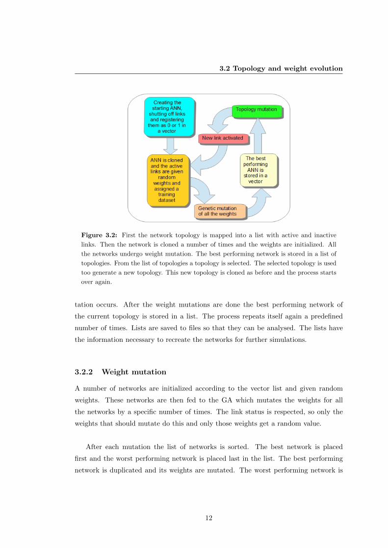
Figure 3.2: First the network topology is mapped into a list with active and inactive

links. Then the network is cloned a number of times and the weights are initialized. All

the networks undergo weight mutation. The best performing network is stored in a list of

topologies. From the list of topologies a topology is selected. The selected topology is used

too generate a new topology. This new topology is cloned as before and the process starts

over again.

tation occurs. After the weight mutations are done the best performing network of

the current topology is stored in a list. The process repeats itself again a predefined

number of times. Lists are saved to files so that they can be analysed. The lists have

the information necessary to recreate the networks for further simulations.

3.2.2 Weight mutation

A number of networks are initialized according to the vector list and given random

weights. These networks are then fed to the GA which mutates the weights for all

the networks by a specific number of times. The link status is respected, so only the

weights that should mutate do this and only those weights get a random value.

After each mutation the list of networks is sorted. The best network is placed

first and the worst performing network is placed last in the list. The best performing

network is duplicated and its weights are mutated. The worst performing network is

12

3.3 Simulation parameters

thrown away.

Topology generation occurs a predefined number of times and after a fixed number

of weight mutations the learning parameter σvar (see section 3.3) is decreased. When

the predefined number of mutations are reached then the process starts over again after

a new topology mutation has taken place.

All the weights are updated by the following equation

w = w + (2 · r − 1)σvar

Where w is the weight that is updated, the random number r generated is between 0-1.

The learning rate σvar is initialized to lr and changes by a factor δ0 = 0.85 - which was

found to be a good value. The σvar parameter changes after every ξ0 weight mutations.

3.3 Simulation parameters

The simulation parameters are presented in the bullet list below and have different

importance depending on the training method used.

• Method for topology selection. There are 6 methods available for mutating the

topology.

• Total network population. Will be used for weight mutation. (N0)

• Maximal topology. Specifying a vector of integers with the number of input nodes,

hidden nodes and output nodes.

• Maximum number of genetic mutations (mutating the weights). (GM)

• Maximum number of topology mutations. (TM)

• Initial learning rate. (lr)

• Periodic change of the initial learning rate. After a number of ξ0 weight mutations

lr is changed. (ξ0)

13

3.4 Topology selection methods

• Change of the initial learning rate. When ξ0 weight mutations have occurred then

lr is changed by a factor δ0 that is between 0 and 1. (δ0)

3.4 Topology selection methods

The parameter settings will affect the topology diversity. To keep track of the different

topologies two different lists are used. One list stores all the topologies. The other list is

used to evaluate the current topology undergoing weight mutation. Different methods

for topology selection and weight mutation strategies are developed and studied.

All the methods choose the best performing network on validation among the cur-

rent topology. This topology is then stored in a list and from that list the networks

are then chosen to be further mutated (see section 3.2.1). Below follows a list of the

available methods for topology selection.

1. Chooses a random network or the first network.

2. Chooses the first network or the last network.

3. Selects randomly a network from the list of topologies.

4. Chooses only the last network which means continuous mutation of the topology.

5. Chooses the first network with if

r · iTM2

TM≤ 1

where r is a random number between 0-1, iTM is the topology iterator, TM is

the total number of topology mutations that was specified in the beginning of the

simulation. If the condition is not met then a random topology from the topology

list is chosen. This gives much more diversity among the topologies and means it

will have a larger possibility to find a network that generalizes well. But the same

14

3.5 The dataset

mutation can for example occur twice. That topology will have a higher prob-

ability of being chosen later. For simplicity we do not look for topology duplicates.

6. Works the same way as method 5 except that after one third of the TM is done

then the networks whose topology has at most mutated once are disregarded.

This method will enhance the development of the network complexity, compared

to the fifth method.

3.5 The dataset

Our implementations of the TWEANN was applied to the Pima Indian dataset[4] prob-

lem. The dataset had 8 inputs and 1 output. Size of the dataset was 768 data points.

The dataset was split up in two parts, 70% training and 30% validation. The scope

was to classify if the Pima Indians had diabetes and should be treated or not. In our

simulations, each input is normalised so that the highest absolute value is 1.

3.6 Simple test case

The code for developing the topology was integrated with the weight mutation. This

was tested by trying to solve the XOR problem. The XOR problem is a simple test

where the ANN has to classify two data points of each type. The data points make up

a quadratic shape and same type of data points are positioned at opposite corners. The

two inputs and output for the XOR problem are as follows, {0, 0, 1; 0, 1, 0; 1, 0, 0; 1, 1, 1}.The XOR problem is a non-linear problem.

The XOR problem was used to test our implementation of the BTWEANN code.

From the beginning the ANN did not have the necessary nodes or connections to solve

the XOR problem. Then it had the nodes needed but was underdeveloped and not

allowed to evolve, so there were to few connections. The final stage was to let the ANN

evolve its topology and show that it can solve the XOR problem.

15

4

Results

The data points seen in the coming graphs represent the training and/or the validation

result of a specific topology.Now we present the Pima Indian problem. All the figures

deal with the Pima Indian data set. The same topology may occur more than once and

can give different results depending on the weight configuration of the ANN.

4.1 Suitable parameter settings

The parameters have to be adjusted so that the networks perform well enough. After

the parameters have been adjusted then it can be studied how different topologies and

complexity affects overtraining. The parameters that are being adjusted are the initial

learning rate lr, the number of weight mutations GM , the population size N0, the

frequency of change of the learning rate ξ0 and the change of lr that works well has

been found to be δ0 = 0.85.

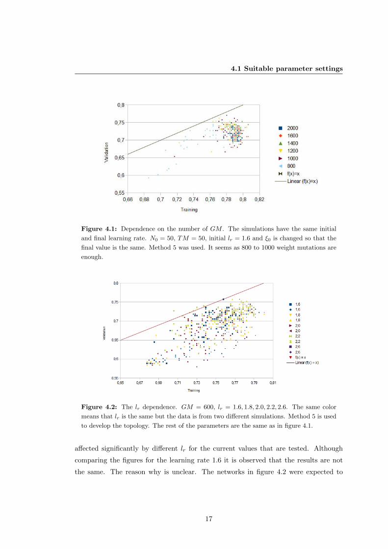
In figure 4.1 it is shown what happens if the number of genetic mutations are var-

ied. The higher the GM is the better the result until a certain value, see figure 4.1.

Fewer than 800 mutations results in networks that are not performing well enough, see

the data points for GM = 800 in figure 4.1. More than 1000 GM should result in

a higher frequency of networks becoming overtrained. The value of weight mutations

GM , needed to get a good enough result for the data set used is about 800-1000.

If parameters are almost the same then it is expected that simulation results should

be similar. In figures 4.2 and 4.3 lr is varied. The figures show that the result is not

16

4.1 Suitable parameter settings

Figure 4.1: Dependence on the number of GM . The simulations have the same initial

and final learning rate. N0 = 50, TM = 50, initial lr = 1.6 and ξ0 is changed so that the

final value is the same. Method 5 was used. It seems as 800 to 1000 weight mutations are

enough.

Figure 4.2: The lr dependence. GM = 600, lr = 1.6, 1.8, 2.0, 2.2, 2.6. The same color

means that lr is the same but the data is from two different simulations. Method 5 is used

to develop the topology. The rest of the parameters are the same as in figure 4.1.

affected significantly by different lr for the current values that are tested. Although

comparing the figures for the learning rate 1.6 it is observed that the results are not

the same. The reason why is unclear. The networks in figure 4.2 were expected to

17

4.1 Suitable parameter settings

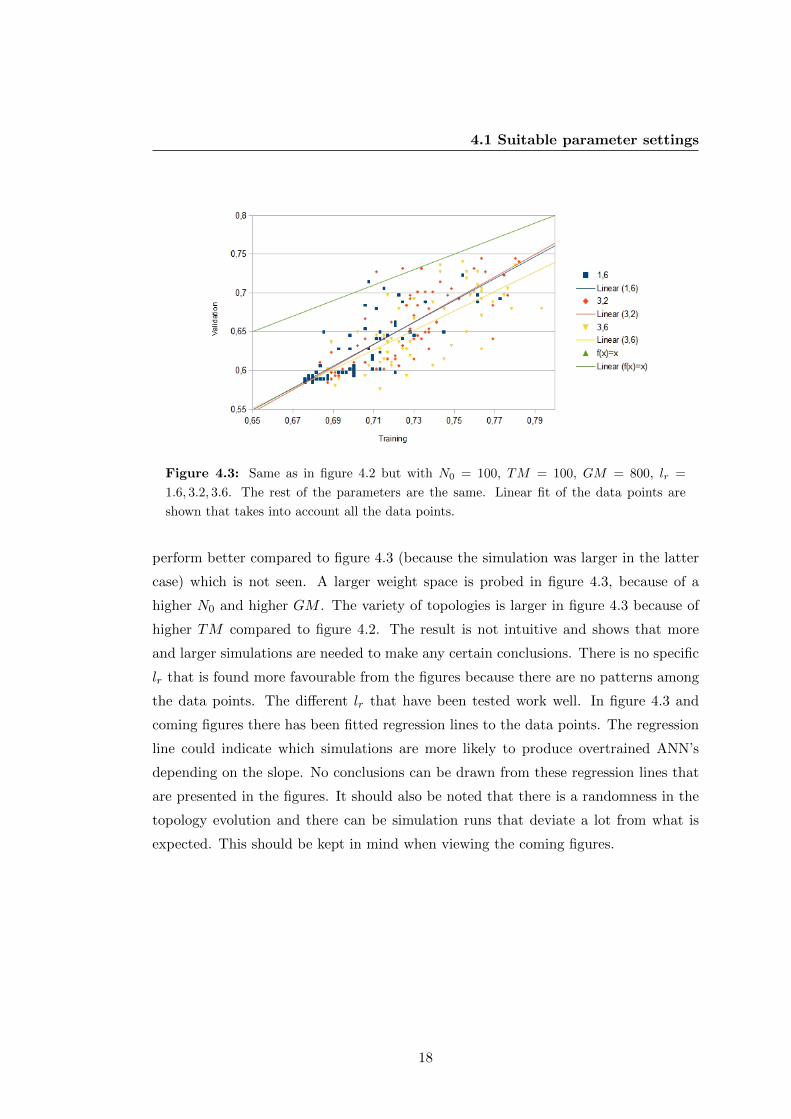
Figure 4.3: Same as in figure 4.2 but with N0 = 100, TM = 100, GM = 800, lr =

1.6, 3.2, 3.6. The rest of the parameters are the same. Linear fit of the data points are

shown that takes into account all the data points.

perform better compared to figure 4.3 (because the simulation was larger in the latter

case) which is not seen. A larger weight space is probed in figure 4.3, because of a

higher N0 and higher GM . The variety of topologies is larger in figure 4.3 because of

higher TM compared to figure 4.2. The result is not intuitive and shows that more

and larger simulations are needed to make any certain conclusions. There is no specific

lr that is found more favourable from the figures because there are no patterns among

the data points. The different lr that have been tested work well. In figure 4.3 and

coming figures there has been fitted regression lines to the data points. The regression

line could indicate which simulations are more likely to produce overtrained ANN’s

depending on the slope. No conclusions can be drawn from these regression lines that

are presented in the figures. It should also be noted that there is a randomness in the

topology evolution and there can be simulation runs that deviate a lot from what is

expected. This should be kept in mind when viewing the coming figures.

18

4.1 Suitable parameter settings

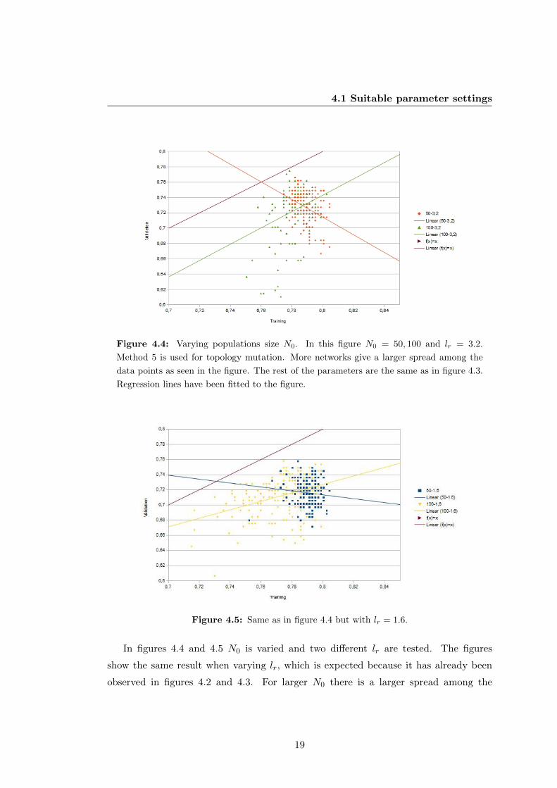
Figure 4.4: Varying populations size N0. In this figure N0 = 50, 100 and lr = 3.2.

Method 5 is used for topology mutation. More networks give a larger spread among the

data points as seen in the figure. The rest of the parameters are the same as in figure 4.3.

Regression lines have been fitted to the figure.

Figure 4.5: Same as in figure 4.4 but with lr = 1.6.

In figures 4.4 and 4.5 N0 is varied and two different lr are tested. The figures

show the same result when varying lr, which is expected because it has already been

observed in figures 4.2 and 4.3. For larger N0 there is a larger spread among the

19

4.1 Suitable parameter settings

performance of the networks as is seen in figures 4.4 and 4.5. Higher TM produces

a larger pool of simple ANN that have only one topology mutation, because method

5 is used for evolving the topology (see section 3.4). The data points for N0 = 100

will have a larger spread in its weight configurations because there are more networks

compared to N0 = 50. The reason why the data points are spread out needs to be

further investigated. If the complexity of the ANN is too simple then it cannot solve

the problem. These topologies should be the ones in the lower left corner of figures

4.4 and 4.5. Leaving out some of the data results that are part of the initial pool of

topologies might show a better result.

Figure 4.6: The data points show no bigger difference depending on the variation in ξ0.

Although the yellow points are less spread out compared to the blue. N0 = 100, lr = 3.6,

GM = 800, TM = 100. Method 5 is used.

In figure 4.6 it is shown how the performance changes when varying ξ0. It is difficult

to say that varying ξ0 shows much of a difference in figure 4.6. It was expected that

varying ξ0 would have a larger impact on the network performance because ξ0 affects

how much the network weights change. For ξ0 = 40 there seems to be a larger spread

compared to ξ0 = 160 but it is not conclusive. Figure 4.6 indicates that ξ0 can be

estimated by considering ξ0 being 4− 16% of the total GM .

20

4.2 Performance and complexity

4.2 Performance and complexity

Figure 4.7: Results obtained with methods 1, 2, 3 and 6. N0 = 100, lr = 3.2, GM = 800,

TM = 100 and ξ0 = 50.

In figure 4.7 different methods that have been developed are tested. The parameter

settings are determined from the parameter tests made in the figures before. Method

1 in figure 4.7 is not performing that well because most of the data points are in the

lower left corner of the figure. The reason could be many simple topologies and the

networks that get complex are not performing well because the connections between

the nodes are inadequate. The networks that are mutated according to method 3 tend

to get more overtrained and perform quite well on validation. Method 2 and 6 are

less overtrained than method 3 and they perform equally well on validation, at a high

frequency. All methods, except method 1, has a good spread in the upper right and

potential of finding a good ANN. The methods that avoid choosing the first topology

seem to produce networks that perform better. Generating more complex topologies is

expected to enhance the performance of the networks.

Figure 4.7 and 4.8 shows one simulation run for each method and to get a clearer

and more general result more and bigger simulations are needed. The complexity of the

ANN’s are very different in figure 4.8 depending on the method. Therefore it is difficult

to say if there is any particular pattern in the development of complexity depending

21

4.2 Performance and complexity

Figure 4.8: Developing complexity depending on method. Same as in figure 5.10 but

now showing the development of complexity during the simulation. The y-axis shows how

many links are active. The x-axis shows TM .

on the method used. Method 1 and 2 tend to get less complex in general. Method

3 chooses randomly and it is seen that this method generates ANN’s that are getting

more complex and fluctuating a lot. The fluctuations were expected because a very

simple or complex ANN could be chosen for the next mutation. Method 6 should gen-

erate more complex ANN’s at the end and does so but it seems that method 3 has more

success at generating more complex ANN’s. Method 6 is not fully developed because

the question is how much time during the simulation should be dedicated to developing

the complexity. When the ANN gets complex it can happen that the way the nodes

are connected do not favour a good performance.

Figure 4.9 shows how data points from several runs that are grouped together like

an oval shaped form. This simulation investigated the stability of the results, since the

results of one run does not affect future runs. If some parameter values are tweaked a

bit then the data points might move a little upwards to the right and spread out a bit

more. These parameters could be any of the parameters that are stated in the figure

text for figure 4.9.

22

4.2 Performance and complexity

Figure 4.9: Testing stability of ten different runs. The 10 results are plotted together in

the figure. All the parameters are the same for each simulation run. N0 = 100, lr = 3.2,

GM = 1000, TM = 150 and ξ0 = 30. The fifth method is used.

Figure 4.10: Performance depending on complexity. The first simulation run from figure

4.9. On the x-axis is the complexity. On the y-axis is the performance of the ANN.

In figure 4.10 the training and validation is affected by the network topology. Dif-

ferent topologies with the same complexity shows that the performance is affected. It

cannot be seen which training and validation result that belongs together in figure 4.10

23

4.2 Performance and complexity

but that is not of importance here. What is important and should be noted is that the

connection between the nodes makes a difference on the performance.

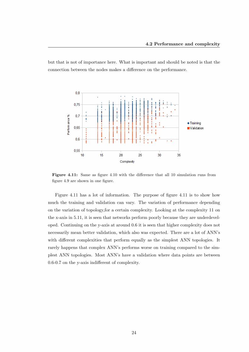
Figure 4.11: Same as figure 4.10 with the difference that all 10 simulation runs from

figure 4.9 are shown in one figure.

Figure 4.11 has a lot of information. The purpose of figure 4.11 is to show how

much the training and validation can vary. The variation of performance depending

on the variation of topology,for a certain complexity. Looking at the complexity 11 on

the x-axis in 5.11, it is seen that networks perform poorly because they are underdevel-

oped. Continuing on the y-axis at around 0.6 it is seen that higher complexity does not

necessarily mean better validation, which also was expected. There are a lot of ANN’s

with different complexities that perform equally as the simplest ANN topologies. It

rarely happens that complex ANN’s performs worse on training compared to the sim-

plest ANN topologies. Most ANN’s have a validation where data points are between

0.6-0.7 on the y-axis indifferent of complexity.

24

4.2 Performance and complexity

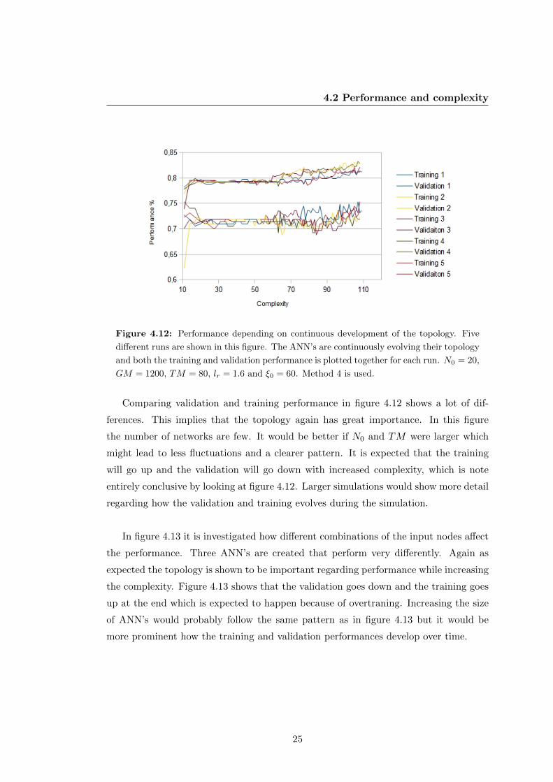
Figure 4.12: Performance depending on continuous development of the topology. Five

different runs are shown in this figure. The ANN’s are continuously evolving their topology

and both the training and validation performance is plotted together for each run. N0 = 20,

GM = 1200, TM = 80, lr = 1.6 and ξ0 = 60. Method 4 is used.

Comparing validation and training performance in figure 4.12 shows a lot of dif-

ferences. This implies that the topology again has great importance. In this figure

the number of networks are few. It would be better if N0 and TM were larger which

might lead to less fluctuations and a clearer pattern. It is expected that the training

will go up and the validation will go down with increased complexity, which is note

entirely conclusive by looking at figure 4.12. Larger simulations would show more detail

regarding how the validation and training evolves during the simulation.

In figure 4.13 it is investigated how different combinations of the input nodes affect

the performance. Three ANN’s are created that perform very differently. Again as

expected the topology is shown to be important regarding performance while increasing

the complexity. Figure 4.13 shows that the validation goes down and the training goes

up at the end which is expected to happen because of overtraning. Increasing the size

of ANN’s would probably follow the same pattern as in figure 4.13 but it would be

more prominent how the training and validation performances develop over time.

25

4.2 Performance and complexity

Figure 4.13: Same as in figure 4.12. In this figure N0 = 100, TM = 200, GM = 1000,

lr = 3.2 and ξ0 = 100. It is observed that the complexity affects the performance. The

mean value result of three different simulation runs are shown.

26

5

Discussion & Outlook

5.1 The Pima Indian dataset

In this thesis we successfully implemented topology evolution. The performance was

investigated using the Pima Indian dataset as a test bed. The Pima Indian dataset

represents a computational challenge. Nevertheless we can see some trends in the re-

sults.

Investigating different strategies for topology development and how it affects over-

training was the goal of this work. It was found that the topology plays a vital role in

how the network performs according to the figures 4.12 and 4.13. Different methods

have been developed for the purpose of improving the performance and study topology

development. Topologies show different amounts of overtraining by comparing topolo-

gies with same the complexity (see figure 4.11). Overtraining is affected by complexity

and by the topology. Continuous development of the topology indicates overtraining.

There are indications that user defined parameters like GM affects the performance

quite a lot (see figure 4.1). Also there are certain behaviours that arise when different

parameters are varied such as ξ0 and GM but these are not conclusive.

27

5.2 The possibilities

5.2 The possibilities

The topology mutation occurs randomly. Also the performance will not affect the fu-

ture development of the network topologies during simulation. however influencing the

selection process in the topology space was not the aim of this project.

The method of developing the topology is very important. A key factor is that the

diversity needs to be large. If the diversity is not large then some topologies will be

favoured by having a higher probability of being selected for topology mutation. It is a

difficult problem to optimize the search in topology space. One possibility is to look at

what similarities there are between the best and worst performing topologies regard-

ing validation. Meta-optimization of the topology would further increase performance.

In this approach knowledge from earlier simulations regarding favourable topologies is

used to further optimize the search in topology space.

The topology development can be done more efficiently. By using different methods

of restrictions to avoid the same topology appearing again and also lobotomising the

network if needed to go back to the better-less-complex topology. Then try to activate

another link that might be more promising. Trying to stop training when the perfor-

mance is decreasing is also common to use. Another way of increasing efficiency when

selecting topologies is by throwing away topologies that do not perform better than

some average performance and replace them, thereby ensuring that the possibility of

evolving depends on performance. Computational time will be saved and there will be

more time to explore unique topology architectures and weight configurations.

Selecting topologies entirely based on performance can have a downside. Topologies

that have developed but are missing some combination between the links can become

one of the best topologies for solving the problem. The poorly performing topologies

need to get a chance to evolve. Giving the chance for some poorly performing topologies

to evolve further can be done by protecting them. The protection of topologies can be

done by giving some networks immunity from being thrown away. This immunity can

be based on the topology mutation iterator. After a number of mutations the topology

will be vulnerable again. Using this kind of approach to protect certain networks will

28

5.2 The possibilities

require a list that has to be updated regularly and might be computationally demand-

ing.

Lastly it is important to say that it is difficult to make any precise conclusions from

the figures shown in the result section. More and larger simulation runs are needed so

that statistically satisfactory results can be acquired. The classification performance

was not satisfactory but the findings in this work does answer an important question.

Topology plays a vital role in the performance of the ANN.

29

Bibliography

[1] S. Haykin, Neural Networks and Learning Machines (Pearson Prentice Hall, 3rd

edition, 2009)

[2] K.O. Stanley and R. Miikkulainen, Evolving Neural Networks through Augmenting

Topologies, Evolutionary Computation 10, 99-127 (2002)

[3] D.J. Montana and L. Davis, Training Feedforward Neural Networks Using Genetic

Algorithms, In Proceedings of the International Joint Conference on Artificial

Intelligence, pp. 762-767 (1989)

[4] J.W. Smith, J.E. Everhart, W.C. Dickson, W.C. Knowler and R.S. Johannes,

Using the ADAP learning algorithm to forecast the onset of diabetes mellitus, In

Proceedings of the Symposium on Computer Applications and Medical Care, pp.

261-265 (1988)

[5] http://neuroph.sourceforge.net/

30