Springer Series in Optical Sciences 181

Valerii (Vartan) Ter-Mikirtychev

Fundamentals of Fiber Lasers and Fiber Amplifiers

Springer Series in Optical Sciences

Volume 181

Founded by

H. K. V. Lotsch

Editor-in-Chief

W. T. Rhodes

Editorial Board

Ali Adibi, AtlantaToshimitsu Asakura, SapporoTheodor W. Hänsch, GarchingTakeshi Kamiya, TokyoFerenc Krausz, GarchingBo A. J. Monemar, LinköpingHerbert Venghaus, BerlinHorst Weber, BerlinHarald Weinfurter, München

For further volumes:http://www.springer.com/series/624

Springer Series in Optical Sciences

The Springer Series in Optical Sciences, under the leadership of Editor-in-Chief William T. Rhodes,Georgia Institute of Technology, USA, provides an expanding selection of research monographs in allmajor areas of optics: lasers and quantum optics, ultrafast phenomena, optical spectroscopy techniques,optoelectronics, quantum information, information optics, applied laser technology, industrial appli-cations, and other topics of contemporary interest.

With this broad coverage of topics, the series is of use to all research scientists and engineers who needup-to-date reference books.

The editors encourage prospective authors to correspond with them in advance of submitting a man-uscript. Submission of manuscripts should be made to the Editor-in-Chief or one of the Editors. See alsowww.springer.com/series/624

Editor-in-ChiefW. T. RhodesSchool of Electrical and Computer EngineeringGeorgia Institute of TechnologyAtlanta, GA 30332-0250USAe-mail: bill.rhodes@ece.gatech.edu

Editorial BoardAli AdibiGeorgia Institute of TechnologySchool of Electrical and Computer EngineeringAtlanta, GA 30332-0250USAe-mail: adibi@ee.gatech.edu

Toshimitsu AsakuraFaculty of EngineeringHokkai-Gakuen University1-1, Minami-26, Nishi 11, Chuo-kuSapporo, Hokkaido 064-0926, Japane-mail: asakura@eli.hokkai-s-u.ac.jp

Theodor W. HänschMax-Planck-Institut für QuantenoptikHans-Kopfermann-Straße 185748 Garching, Germanye-mail: t.w.haensch@physik.uni-muenchen.de

Takeshi KamiyaMinistry of Education, Culture, SportsScience and TechnologyNational Institution for Academic Degrees3-29-1 Otsuka Bunkyo-kuTokyo 112-0012, Japane-mail: kamiyatk@niad.ac.jp

Ferenc KrauszLudwig-Maximilians-Universität MünchenLehrstuhl für Experimentelle PhysikAm Coulombwall 185748 Garching, Germany andMax-Planck-Institut für QuantenoptikHans-Kopfermann-Straße 185748 Garching, Germanye-mail: ferenc.krausz@mpq.mpg.de

Bo A. J. MonemarDepartment of Physics and Measurement TechnologyMaterials Science DivisionLinköping University58183 Linköping, Swedene-mail: bom@ifm.liu.se

Herbert VenghausFraunhofer Institut für NachrichtentechnikHeinrich-Hertz-InstitutEinsteinufer 3710587 Berlin, Germanye-mail: venghaus@hhi.de

Horst WeberOptisches InstitutTechnische Universität BerlinStraße des 17. Juni 13510623 Berlin, Germanye-mail: weber@physik.tu-berlin.de

Harald WeinfurterSektion PhysikLudwig-Maximilians-Universität MünchenSchellingstraße 4/III80799 München, Germanye-mail: harald.weinfurter@physik.uni-muenchen.de

Valerii (Vartan) Ter-Mikirtychev

Fundamentals of FiberLasers and Fiber Amplifiers

123

Valerii (Vartan) Ter-MikirtychevMountain View, CAUSA

ISSN 0342-4111 ISSN 1556-1534 (electronic)ISBN 978-3-319-02337-3 ISBN 978-3-319-02338-0 (eBook)DOI 10.1007/978-3-319-02338-0Springer Cham Heidelberg New York Dordrecht London

Library of Congress Control Number: 2013948738

� Springer International Publishing Switzerland 2014This work is subject to copyright. All rights are reserved by the Publisher, whether the whole or part ofthe material is concerned, specifically the rights of translation, reprinting, reuse of illustrations,recitation, broadcasting, reproduction on microfilms or in any other physical way, and transmission orinformation storage and retrieval, electronic adaptation, computer software, or by similar or dissimilarmethodology now known or hereafter developed. Exempted from this legal reservation are briefexcerpts in connection with reviews or scholarly analysis or material supplied specifically for thepurpose of being entered and executed on a computer system, for exclusive use by the purchaser of thework. Duplication of this publication or parts thereof is permitted only under the provisions ofthe Copyright Law of the Publisher’s location, in its current version, and permission for use mustalways be obtained from Springer. Permissions for use may be obtained through RightsLink at theCopyright Clearance Center. Violations are liable to prosecution under the respective Copyright Law.The use of general descriptive names, registered names, trademarks, service marks, etc. in thispublication does not imply, even in the absence of a specific statement, that such names are exemptfrom the relevant protective laws and regulations and therefore free for general use.While the advice and information in this book are believed to be true and accurate at the date ofpublication, neither the authors nor the editors nor the publisher can accept any legal responsibility forany errors or omissions that may be made. The publisher makes no warranty, express or implied, withrespect to the material contained herein.

Printed on acid-free paper

Springer is part of Springer Science+Business Media (www.springer.com)

Dedicated in memory of my parents Vartanand Vera,and to my wife Katerinaand my children William and Daria

Acknowledgments

I would like to thank my former and current colleagues in Russia, Japan, and USAfor useful discussion on many topics of laser physics in general and fiber opticsand fiber lasers in particular. I am indebted to Dr. P. Silfsten, Prof. T. Kurobori,Prof. K. Ueda, Dr. V. Kozlov, Prof. E. Sviridenkov, Dr. M. Dubinskii,Dr. V. Fromzel, Dr. J. Zhang, Dr. N. Klaus, Dr. S. Fuerstenau, Dr. I. McKinnie,Mr. P. Ishkanian, and Prof. J.-W. Ryu, for useful and interesting discussions. I amalso glad to have an opportunity to thank Mr. M. O’Connor of IPG, Mr. W. Wilsonof Liekki/nLight, and Mr. D. Beiko of CorActive for many useful discussions oncommercially available fibers.

I am thankful to my teachers and former colleagues at Moscow Physics andEngineering Institute (MEPhI), P. N. Lebedev Physical Institute (LPI) of theRussian Academy of Sciences, and A. M. Prokhorov General Physics Institute(GPI) of the Russian Academy of Sciences (RAS), namely: the late Prof.Yu. A. Bykovskii, Prof. E. D. Protcenko, Prof. E. A. Sviridenkov, late Prof. A. N.Oraevsky, Prof. Yu. M. Popov, the late Prof. A. P. Shotov, Prof. V. G. Sheretov (TverState University), and late Prof. A. G. Avanesov (Krasnodar State University). Also,Prof. V. P. Danilov, Prof. V. A. Smirnov. and Academician Prof. I. A. Shcherbakov,President of A. M. Prokhorov GPI RAS.

Further, I would like to express my personal gratitude to the organizer of theSpecial Physics Department of MEPhI where I had a privilege to be educated andwhat in turn made several important changes in my life and who served as a boardChair of my graduation exams, i.e., former director of P. N. Lebedev PhysicalInstitute the late Academician Prof. N. G. Basov, 1964 Nobel Prize Laureatein Physics (together with the late Academician Prof. A. M. Prokhorov and Prof.C. H. Townes).

Special thanks go to Mr. Stuart McLean, a fiber laser engineer, who did the hardwork of proofreading the whole manuscript and whose suggestions definitelyimproved the material presentation. Additionally, I give thanks to Mr. WilliamTerson for partial proofreading of the manuscript. I also highly appreciate the helpof Springer Physics Editor Mr. Christopher Caughlin, and Mr. Ho Ying Fan, bothfrom Springer for their constant help and assistance throughout the whole projectincluding manuscript preparation and publication.

vii

Finally, but not less importantly, I would like to thank my wife Katerina who isa Fiber-Optic engineer herself for her helpful suggestions including technical andstylistic, constant support and encouraging. Appearance of this book withoutKaterina’s support would be impossible.

viii Acknowledgments

Contents

1 Introduction . . . . . . . . . . . . . . . . . . . . . . . . . . . . . . . . . . . . . . . . 1References . . . . . . . . . . . . . . . . . . . . . . . . . . . . . . . . . . . . . . . . . 5

2 Optical Properties and Optical Spectroscopy of Rare EarthIons in Solids . . . . . . . . . . . . . . . . . . . . . . . . . . . . . . . . . . . . . . . 72.1 Electron–Phonon Coupling in Solids . . . . . . . . . . . . . . . . . . . 72.2 Phonon Sidebands of Optical Transition in Solids . . . . . . . . . 92.3 Optical Center Transitions: Spontaneous

and Stimulated Emission . . . . . . . . . . . . . . . . . . . . . . . . . . . 102.4 Rare Earth Centers in Solids . . . . . . . . . . . . . . . . . . . . . . . . 132.5 Homogeneous and Inhomogeneous Line Broadening. . . . . . . . 14

2.5.1 Homogeneous Broadening . . . . . . . . . . . . . . . . . . . 142.5.2 Inhomogeneous Broadening . . . . . . . . . . . . . . . . . . 16

2.6 Spectroscopic Parameters of the Optical Transition:A Brief Introduction to the Main Theories. . . . . . . . . . . . . . . 172.6.1 Judd–Ofelt Theory . . . . . . . . . . . . . . . . . . . . . . . . 182.6.2 McCumber Theory . . . . . . . . . . . . . . . . . . . . . . . . 192.6.3 Füchtbauer–Ladenburg Theory and Einstein

Coefficients . . . . . . . . . . . . . . . . . . . . . . . . . . . . . 212.7 Sensitization of Laser-Active Centers . . . . . . . . . . . . . . . . . . 23References . . . . . . . . . . . . . . . . . . . . . . . . . . . . . . . . . . . . . . . . . 25

3 Physical and Optical Properties of Laser Glass . . . . . . . . . . . . . . 273.1 Mechanical and Thermal Properties of Glass . . . . . . . . . . . . . 283.2 Optical Properties of Fibers (Attenuation) . . . . . . . . . . . . . . . 30

3.2.1 Intrinsic Glass Material Properties . . . . . . . . . . . . . 303.2.2 Waveguide Properties . . . . . . . . . . . . . . . . . . . . . . 313.2.3 Optical Connection Loss . . . . . . . . . . . . . . . . . . . . 32

3.3 Different Glass Types Used in Fiber Lasers and Amplifiers. . . 323.3.1 Silicate Glass . . . . . . . . . . . . . . . . . . . . . . . . . . . . 333.3.2 Phosphate Glass . . . . . . . . . . . . . . . . . . . . . . . . . . 343.3.3 Tellurite Glass . . . . . . . . . . . . . . . . . . . . . . . . . . . 343.3.4 Fluoride Glass and ZBLAN . . . . . . . . . . . . . . . . . . 34

References . . . . . . . . . . . . . . . . . . . . . . . . . . . . . . . . . . . . . . . . . 36

ix

4 Fiber Fabrication and High-Quality Glasses for Gain Fibers . . . . 374.1 Materials . . . . . . . . . . . . . . . . . . . . . . . . . . . . . . . . . . . . . . 374.2 Fabrication of Fiber Preforms . . . . . . . . . . . . . . . . . . . . . . . 374.3 Fiber Fabrication from the Preform. . . . . . . . . . . . . . . . . . . . 394.4 Laser-Active Fiber Fabrication . . . . . . . . . . . . . . . . . . . . . . . 394.5 MCVD Technology for Rare-Earth Doped

Fiber Production. . . . . . . . . . . . . . . . . . . . . . . . . . . . . . . . . 404.6 DND Technology . . . . . . . . . . . . . . . . . . . . . . . . . . . . . . . . 42References . . . . . . . . . . . . . . . . . . . . . . . . . . . . . . . . . . . . . . . . . 42

5 Spectroscopic Properties of Nd31, Yb31, Er31,and Tm31 Doped Fibers . . . . . . . . . . . . . . . . . . . . . . . . . . . . . . . 435.1 Spectroscopic Notations . . . . . . . . . . . . . . . . . . . . . . . . . . . 435.2 Energy Levels of Trivalent Rare Earth Ions . . . . . . . . . . . . . . 445.3 Neodymium . . . . . . . . . . . . . . . . . . . . . . . . . . . . . . . . . . . . 45

5.3.1 Nd3? Fiber Laser Challenges . . . . . . . . . . . . . . . . . 495.4 Ytterbium . . . . . . . . . . . . . . . . . . . . . . . . . . . . . . . . . . . . . 50

5.4.1 Yb3? Fiber Laser Challenges . . . . . . . . . . . . . . . . . 515.5 Erbium . . . . . . . . . . . . . . . . . . . . . . . . . . . . . . . . . . . . . . . 53

5.5.1 Er3? Fiber Laser Challenges . . . . . . . . . . . . . . . . . 565.6 Thulium . . . . . . . . . . . . . . . . . . . . . . . . . . . . . . . . . . . . . . 57

5.6.1 Tm3? Fiber Laser Challenges . . . . . . . . . . . . . . . . . 59References . . . . . . . . . . . . . . . . . . . . . . . . . . . . . . . . . . . . . . . . . 62

6 Propagation of Light and Modes in Optical Fibers . . . . . . . . . . . 656.1 V Number of the Fiber . . . . . . . . . . . . . . . . . . . . . . . . . . . . 666.2 Fiber Dispersion . . . . . . . . . . . . . . . . . . . . . . . . . . . . . . . . . 686.3 Polarization-Maintaining Fibers . . . . . . . . . . . . . . . . . . . . . . 726.4 Laser Beam Quality (M2 Parameter) . . . . . . . . . . . . . . . . . . . 73

6.4.1 Practical Recommendations on Beam QualityMeasurements Using the M2 Approach . . . . . . . . . . 75

References . . . . . . . . . . . . . . . . . . . . . . . . . . . . . . . . . . . . . . . . . 77

7 Fiber Laser Physics Fundamentals . . . . . . . . . . . . . . . . . . . . . . . 797.1 Population Inversion: Three- and Four-EnergyLevel

Systems. . . . . . . . . . . . . . . . . . . . . . . . . . . . . . . . . . . . . . . 797.1.1 Four-Level Laser Operational Scheme. . . . . . . . . . . 807.1.2 Three-Level Laser Operational Scheme . . . . . . . . . . 81

7.2 Optical Fiber Amplifiers . . . . . . . . . . . . . . . . . . . . . . . . . . . 827.2.1 Fiber Amplifier (General Consideration) . . . . . . . . . 82

7.3 Fiber Laser Thresholds and Efficiency . . . . . . . . . . . . . . . . . 907.4 Gain and Loss in Laser Resonators. . . . . . . . . . . . . . . . . . . . 93

x Contents

7.5 Fiber Laser Resonators . . . . . . . . . . . . . . . . . . . . . . . . . . . . 937.5.1 Linear Laser Resonators . . . . . . . . . . . . . . . . . . . . 937.5.2 Ring Laser Resonators. . . . . . . . . . . . . . . . . . . . . . 96

References . . . . . . . . . . . . . . . . . . . . . . . . . . . . . . . . . . . . . . . . . 98

8 Main Operating Regimes of Fiber Lasers . . . . . . . . . . . . . . . . . . 998.1 Temporal Regimes . . . . . . . . . . . . . . . . . . . . . . . . . . . . . . . 99

8.1.1 CW and Free-Running Operation of Fiber Lasers . . . 1008.1.2 Q-Switched Operation of Fiber Lasers. . . . . . . . . . . 1028.1.3 Mode-Locking of Fiber Lasers . . . . . . . . . . . . . . . . 109

8.2 Spectral Regimes . . . . . . . . . . . . . . . . . . . . . . . . . . . . . . . . 1188.2.1 Wavelength Tunable Lasers . . . . . . . . . . . . . . . . . . 1188.2.2 Single Longitudinal Mode Lasers . . . . . . . . . . . . . . 124

References . . . . . . . . . . . . . . . . . . . . . . . . . . . . . . . . . . . . . . . . . 131

9 Main Optical Components for Fiber Laser/Amplifier Design . . . . 1339.1 Laser Diodes . . . . . . . . . . . . . . . . . . . . . . . . . . . . . . . . . . . 133

9.1.1 Principles of Operation . . . . . . . . . . . . . . . . . . . . . 1339.1.2 Main Types of Diode Lasers Used in Fiber Laser

Technology . . . . . . . . . . . . . . . . . . . . . . . . . . . . . 1419.1.3 High-Power Diode Lasers . . . . . . . . . . . . . . . . . . . 1449.1.4 Fiber-Coupled Diode Lasers . . . . . . . . . . . . . . . . . . 148

9.2 Fiber-Coupled Polarization-Maintained andNon-polarization-Maintained Optical Components . . . . . . . . . 1499.2.1 Polarization-Dependent Optical Isolators . . . . . . . . . 1529.2.2 Polarization-Independent Optical Isolators . . . . . . . . 1539.2.3 High-Power Fiber-Coupled Isolators . . . . . . . . . . . . 1549.2.4 Polarization-Dependent Circulator. . . . . . . . . . . . . . 1559.2.5 Polarization-Independent Circulator. . . . . . . . . . . . . 1569.2.6 Chirped FBG as a Self-Phase Modulation

Compensator . . . . . . . . . . . . . . . . . . . . . . . . . . . . 1579.2.7 A Few Words About Fiber Endface Preparation . . . . 159

References . . . . . . . . . . . . . . . . . . . . . . . . . . . . . . . . . . . . . . . . . 160

10 High-Power Fiber Lasers . . . . . . . . . . . . . . . . . . . . . . . . . . . . . . 16110.1 Gain Fiber Pumping Technology for High-Power

Fiber Lasers . . . . . . . . . . . . . . . . . . . . . . . . . . . . . . . . . . . . 16310.2 Double-Clad Fibers and Clad-Pumping Technology . . . . . . . . 164

10.2.1 Clad-Pumping Schemes . . . . . . . . . . . . . . . . . . . . . 16510.2.2 Clad-Pumping and Triple-Clad Fibers . . . . . . . . . . . 16710.2.3 Free Space . . . . . . . . . . . . . . . . . . . . . . . . . . . . . . 16710.2.4 Fused-Pump Combiners . . . . . . . . . . . . . . . . . . . . . 169

10.3 Large-Mode Area Fibers for High-Power,Diffraction-Limited Operation . . . . . . . . . . . . . . . . . . . . . . . 170

Contents xi

10.4 Nonlinear Processes in Optical Fibers and Their Rolein Fiber Laser and Fiber Amplifiers TechnologyDevelopment . . . . . . . . . . . . . . . . . . . . . . . . . . . . . . . . . . . 17210.4.1 Threshold Power of the Stimulated

Scattering Process . . . . . . . . . . . . . . . . . . . . . . . . . 17310.4.2 Stimulated Raman Scattering . . . . . . . . . . . . . . . . . 17410.4.3 Continuous-Wave SRS . . . . . . . . . . . . . . . . . . . . . 17610.4.4 Pulsed SRS . . . . . . . . . . . . . . . . . . . . . . . . . . . . . 17610.4.5 Stimulated Brillouin Scattering . . . . . . . . . . . . . . . . 17710.4.6 Continuous-Wave SBS . . . . . . . . . . . . . . . . . . . . . 17810.4.7 Pulsed SBS . . . . . . . . . . . . . . . . . . . . . . . . . . . . . 18010.4.8 Optical Kerr Effect . . . . . . . . . . . . . . . . . . . . . . . . 18010.4.9 Self-Phase Modulation. . . . . . . . . . . . . . . . . . . . . . 18010.4.10 Cross-Phase Modulation . . . . . . . . . . . . . . . . . . . . 18210.4.11 Four-Wave Mixing . . . . . . . . . . . . . . . . . . . . . . . . 183

10.5 Self-Focusing and Self-Trapping in Optical Fibers . . . . . . . . . 18510.6 High-Power Fiber Laser Oscillators Versus Low-Power

Master Oscillator–Power Fiber Amplifier Geometry . . . . . . . . 18610.6.1 High-Power Fiber Laser Single Oscillators. . . . . . . . 18710.6.2 High-Power Master Oscillator–Power

Fiber Amplifiers . . . . . . . . . . . . . . . . . . . . . . . . . . 18910.7 Beam Combining of High-Power Fiber Lasers . . . . . . . . . . . . 195

10.7.1 Spectral Beam Combining . . . . . . . . . . . . . . . . . . . 19610.7.2 Volume Holographic Grating . . . . . . . . . . . . . . . . . 19710.7.3 Coherent Beam Combining . . . . . . . . . . . . . . . . . . 200

References . . . . . . . . . . . . . . . . . . . . . . . . . . . . . . . . . . . . . . . . . 206

11 Fiber Industrial Applications of Fiber Lasers . . . . . . . . . . . . . . . 20911.1 Laser–Material Interaction for Material Processing . . . . . . . . . 21011.2 Important Laser Parameters for Industrial Application. . . . . . . 212

11.2.1 Wavelength . . . . . . . . . . . . . . . . . . . . . . . . . . . . . 21211.2.2 Pulse Energy . . . . . . . . . . . . . . . . . . . . . . . . . . . . 21211.2.3 Pulse Width and Pulse Repetition Rate . . . . . . . . . . 21311.2.4 Power . . . . . . . . . . . . . . . . . . . . . . . . . . . . . . . . . 21311.2.5 Power Density . . . . . . . . . . . . . . . . . . . . . . . . . . . 21411.2.6 Laser Beam Quality . . . . . . . . . . . . . . . . . . . . . . . 21411.2.7 Spot Diameter . . . . . . . . . . . . . . . . . . . . . . . . . . . 215

11.3 Fiber-Optic Power Delivery Systems. . . . . . . . . . . . . . . . . . . 21511.4 Main Structure of Fiber-Optic Delivery Systems . . . . . . . . . . 22411.5 Main Industrial Applications of Fiber Lasers . . . . . . . . . . . . . 225

11.5.1 Welding. . . . . . . . . . . . . . . . . . . . . . . . . . . . . . . . 22511.5.2 Cutting . . . . . . . . . . . . . . . . . . . . . . . . . . . . . . . . 22611.5.3 Drilling . . . . . . . . . . . . . . . . . . . . . . . . . . . . . . . . 22611.5.4 Soldering . . . . . . . . . . . . . . . . . . . . . . . . . . . . . . . 226

xii Contents

11.5.5 Marking. . . . . . . . . . . . . . . . . . . . . . . . . . . . . . . . 22711.5.6 Heat Treating . . . . . . . . . . . . . . . . . . . . . . . . . . . . 22711.5.7 Metal Deposition . . . . . . . . . . . . . . . . . . . . . . . . . 22711.5.8 Paint Stripping and Surface Removal . . . . . . . . . . . 22711.5.9 Micromachining . . . . . . . . . . . . . . . . . . . . . . . . . . 22811.5.10 Semiconductor Processing with a Laser Beam . . . . . 22811.5.11 Main Competitors of Fiber Lasers in Industrial

Laser Applications . . . . . . . . . . . . . . . . . . . . . . . . 22911.5.12 Summary of Challenges for Fiber Lasers

in Industrial Applications. . . . . . . . . . . . . . . . . . . . 23011.5.13 Future of Fiber Lasers in Material Processing . . . . . 231

References . . . . . . . . . . . . . . . . . . . . . . . . . . . . . . . . . . . . . . . . . 231

12 Conclusion . . . . . . . . . . . . . . . . . . . . . . . . . . . . . . . . . . . . . . . . . 233

Index . . . . . . . . . . . . . . . . . . . . . . . . . . . . . . . . . . . . . . . . . . . . . . . . 235

Contents xiii

Symbols

A21 Einstein A coefficient (probability of spontaneous decay)B12, B21 Einstein B coefficientsb Normalized propagation constantAeff Effective cross-section area of the fiber coreDchrom Chromatic dispersiondnp Depletion region of p-n junctiondn; dp Depletion regions in n- and p-type side of the junctionE EnergyEF Fermi energyF Energy fluencef Oscillator strength of the transitionfF�D E; Tð Þ Fermi function (Fermi–Dirac probability)Fetalon Finesse of the etalong Gain coefficientG Gain factorh Planck constant�h ¼ h

2pReduced Planck constant (or Dirac’s constant)

I Laser intensitykB Boltzmann constantL LengthLeff Effective length of the fiberLlss Large-scale self-focusing characteristic lengthLsss Small-scale self-focusing characteristic lengthLloss Intracavity incidental lossM Number of modesMlens Magnification of the lens systemN ConcentrationNa; Nd Concentration of acceptor and donor impurityDN Population inversion�ni; �nf Normalized population inversionsnth Threshold population inversion

xv

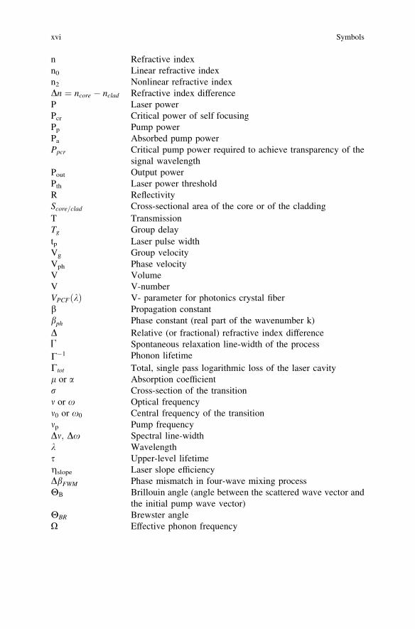
n Refractive indexn0 Linear refractive indexn2 Nonlinear refractive indexDn ¼ ncore � nclad Refractive index differenceP Laser powerPcr Critical power of self focusingPp Pump powerPa Absorbed pump powerPpcr Critical pump power required to achieve transparency of the

signal wavelengthPout Output powerPth Laser power thresholdR ReflectivityScore=clad Cross-sectional area of the core or of the claddingT TransmissionTg Group delaytp Laser pulse widthVg Group velocityVph Phase velocityV VolumeV V-numberVPCFðkÞ V- parameter for photonics crystal fiberb Propagation constantbph Phase constant (real part of the wavenumber k)D Relative (or fractional) refractive index differenceU Spontaneous relaxation line-width of the processC�1 Phonon lifetimeCtot Total, single pass logarithmic loss of the laser cavityl or a Absorption coefficientr Cross-section of the transitionm or x Optical frequencym0 or x0 Central frequency of the transitionmp Pump frequencyDm; Dx Spectral line-widthk Wavelengths Upper-level lifetimegslope Laser slope efficiencyDbFWM Phase mismatch in four-wave mixing processHB Brillouin angle (angle between the scattered wave vector and

the initial pump wave vector)HBR Brewster angleX Effective phonon frequency

xvi Symbols

X2;4;6 Judd–Ofelt parametersc Nonlinear interaction constantK Fiber Bragg grating periodrDC Material DC conductivity

Symbols xvii

Abbreviations

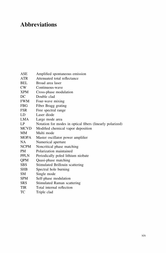
ASE Amplified spontaneous emissionATR Attenuated total reflectanceBEL Broad area laserCW Continuous-waveXPM Cross-phase modulationDC Double cladFWM Four-wave mixingFBG Fiber Bragg gratingFSR Free spectral rangeLD Laser diodeLMA Large mode areaLP Notation for modes in optical fibers (linearly polarized)MCVD Modified chemical vapor depositionMM Multi modeMOPA Master oscillator power amplifierNA Numerical apertureNCPM Noncritical phase matchingPM Polarization maintainedPPLN Periodically poled lithium niobateQPM Quasi-phase matchingSBS Stimulated Brillouin scatteringSHB Spectral hole burningSM Single modeSPM Self-phase modulationSRS Stimulated Raman scatteringTIR Total internal reflectionTC Triple clad

xix

Some of the Most Important FundamentalOptical Constants

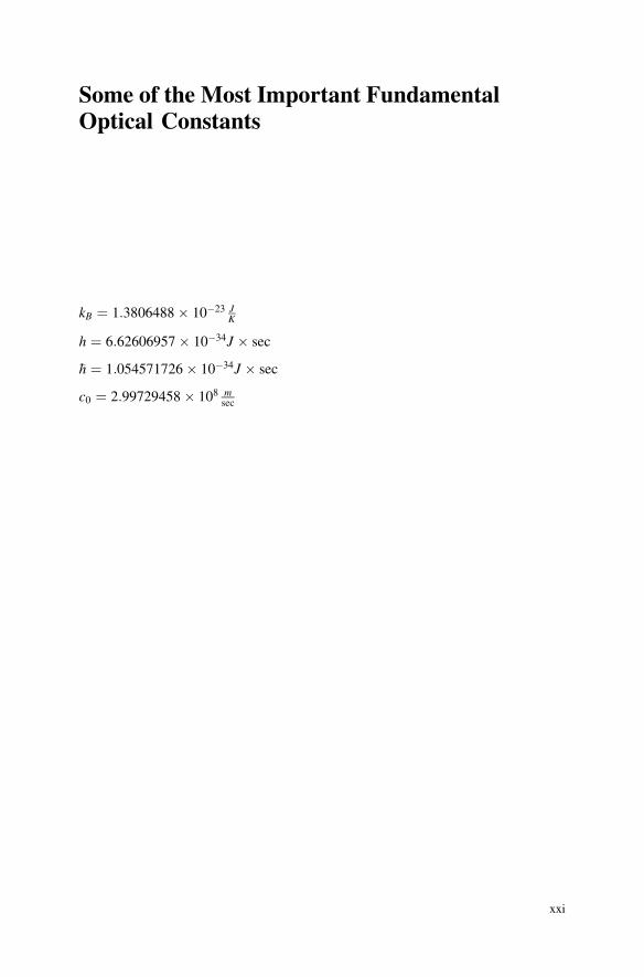
kB ¼ 1:3806488� 10�23 JK

h ¼ 6:62606957� 10�34J � sec

�h ¼ 1:054571726� 10�34J � sec

c0 ¼ 2:99729458� 108 msec

xxi

Chapter 1Introduction

The field of fiber lasers was born in 1961—almost simultaneously with theachievement of the first laser action in Ruby [1]—when Snitzer first published hisfamous paper on laser oscillation in glass [2] and then on the possibility of fiberlaser operation [3]. A few years later, in 1964, Koester and Snitzer experimentallydemonstrated amplification and observed fiber laser oscillation in a gain fiber [4].This important work was followed by other research groups who further studiedfiber lasers. However, great success in the development of other laser-active mediaduring the 1960s and 1970s, such as laser crystals and liquid-dye lasers, as well aslack of availability of diode lasers (the first operation of a diode laser was pub-lished in 1962) put serious fiber laser research on hold for several decades. In the1980s and 1990s, fiber lasers had their second birth due to the appearance ofreasonably powerful and reliable diode lasers and diode-pumped laser technology.This was accompanied by the application of fiber laser technology in opticaltelecommunication, which used a fiber amplifier rather than a fiber laser concept.The basic ideas and discoveries made during the early telecommunication ageplayed—and are still playing—a key role in the development of fiber laser andfiber amplifier systems. The following milestones or achievements should bementioned in the field of fiber lasers and fiber amplifiers as a stand-alone field ofoptics in general and laser physics in particular:

1. First operation of a fiber laser.2. First operation of a fiber amplifier.3. First operation of a diode laser.4. Chemical vapor deposition (and its modifications) fiber fabrication technol-

ogy, which allowed optical fibers to be achieved with extremely low loss.5. Sensitization of some acceptor ions (e.g., Er3+) with donors (e.g., Yb3+).6. Double-clad (DC) fibers and clad pumping technology.7. Development of highly efficient, room-temperature, and cost-effective diode

lasers.8. Development of highly efficient and cost-effective single-frequency diode

lasers.

V. Ter-Mikirtychev, Fundamentals of Fiber Lasers and Fiber Amplifiers,Springer Series in Optical Sciences 181, DOI: 10.1007/978-3-319-02338-0_1,� Springer International Publishing Switzerland 2014

1

9. Significant progress in fiber coupling technology, such as fiber-coupled diodelasers.

10. Development of highly doped gain fibers.11. Commercialization of cost-effective fiber-coupled and all-fiber optical

components.12. Discovery and development of photonic crystal fibers.13. Achievement and development of efficient Raman fiber lasers.14. Development of polarization-maintaining fiber structures.15. Fundamental spatial mode filtering in fibers and coiling technology.

From this list of milestones, one can observe that success in fiber lasers as atechnical field is a result of joint success in the field of solid-state lasers (especiallydiode-pumped lasers) and fiber technology. Accordingly, fiber lasers adoptedtechnological solutions from both of these areas. Today, fiber lasers compete withand threaten to replace most of high-power, bulk solid-state lasers and some gaslasers. The most developed fiber laser systems are based on laser glasses with thefollowing rare earth ions: Yb3+, Er3+, -Yb3+, Tm3+, and Nd3+. Note, however, thathistorically the first ion to be used in fiber laser was the Nd3+ ion; therefore, a lot ofwork has been done using Nd3+ as a laser active ion in fiber laser research,including new operational schemes for unique spectral and temporal fiber lasercharacteristics. Nevertheless, researchers and engineers soon shifted their attentionto Yb3+ and Er3+. Compared with Nd3+, Yb3+ offers higher conversion efficiency,much broader tunability in the 1 lm spectral range, and higher energy storagetime. Later, the advantages of Yb3+ were also magnified by the performance andavailability of the more technological and reliable 9XXnm indium gallium arse-nide (InGaAs) laser diodes used as pumping sources of Yb3+ fiber lasers.

With further advances in the development of diode pump laser technology andoptical telecommunication, other ions such as Er3+ and later Tm3+ received sig-nificant attention from researchers and engineers. This eventually brought powerof the fiber lasers based on these rare earth ions to hundreds of Watts, with morethan 30 % conversion efficiency for Er3+–Yb3+ systems and more than 50 % forEr3+-doped and Tm3+-doped fibers.

Meanwhile, scientists and engineers were investigating ways to significantlyreduce optical loss in fibers. In this direction, the most important technologicalbreakthrough was the discovery of a so-called modified chemical vapor deposition(MCVD, or just CVD) fiber manufacturing technique, which eventually allowedthe achievement of optical fibers with extremely low loss (\*0.2 dB/km in the1.5 lm wavelength range for undoped fibers and 0.01–0.1 dB/m for the rare-earthdoped fibers; i.e., gain fibers). Most fiber preparation processes use MCVDtechnology (or its modifications) as a core process, including gain fiberpreparation.

The next fundamental step towards the development of highly efficient fiberlasers was a proposal to use sensitization of Er3+ laser active ions in glass by Yb3+

ions. Note that in early years of laser research mentioned previously, the Nd3+ ionalso was considered to be a sensitizing ion itself (in this case, for the Yb3+ ion).

2 1 Introduction

This interest, however, was replaced by direct excitation of Yb3+ with theappearance of 9XXnm InGaAs laser diodes. For the Er3+–Yb3+ co-doped system,sensitization makes use of broad absorption of Yb3+ ions in glass at *915 and*976 nm wavelengths, which are accessible by well-developed InGaAs laserdiodes as well as achievable high Yb3+ doping concentration of the laser glass. InEr3+–Yb3+ co-doped material, excited Yb3+ ions in its absorption band have ahighly efficient energy transfer to the Er3+ ions to its upper laser energy level; inturn, this creates a condition for efficient creation of population inversion in Er3+

with subsequent laser action in the *1.5 lm spectral range. The Er3+–Yb3+ sys-tem also plays an important role in double-clad fibers, where achievement ofeffective pump absorption requires longer gain fibers. High concentration of Yb3+

(which in Er3+–Yb3+ laser glass is more than 10 times bigger than that of Er3+)enables efficient high-power pump absorption of the 915 or 976 nm spectral rangein a clad pump geometry, resulting in the achievement of reasonably short DC gainfiber lengths.

As one can imagine, the most technological and scientific efforts (as in the caseof other laser types) have been and are still being placed on the development ofsingle transverse mode fiber lasers and amplifiers operating with close to diffrac-tion-limited beam quality. In the early years of fiber laser development, gain fibersthat support only the fundamental mode had a laser active ion-doped core that wasseveral microns in diameter and an undoped cladding surrounding the core, whichwas usually about 100 lm in diameter. The pump and the signal radiation werelaunched inside the same volume—that is, each into the core from the same oropposite directions of the gain fiber with perfect beam overlap. Although it is agood solution and has several advantages, such core pumping geometry has verylimited power scalability because of the strict requirement for brightness (i.e.,optical power density per divergent solid angle ½W=cm2 � steradian�) of the pumpdiode lasers in order for it to be efficiently launched into the fiber core. Thiscircumstance limited fiber laser power to about a 1 W level at their time, whichcorresponded to the power of single-mode emitter pump diode lasers.

To increase pump power coupled into the gain fiber, in the mid-1980s, severalresearch groups almost simultaneously proposed to launch pump radiation into alarger area of cladding that surrounds a doped core, thus significantly expandingthe capability of launched pump power scaling in fiber lasers. Special fibers havebeen developed for such clad-pump propagation technology. With an externalpolymer coating of a lower refractive index, such fibers allowed simultaneouspropagation of signal radiation inside the core and pump radiation to be guidedinside cladding. Because of this dual wave-guiding property, such fibers are calleddouble-clad fibers—that is, having extra cladding for pump radiation. Note thatbecause of the reduced overlap between the pump area in the clad and theabsorbing area of the core, DC fibers require a longer length for effective pumpabsorption compared with that of core pump fibers with the same core absorptioncoefficient at the pump wavelength. Nevertheless, for high peak power and lowaverage power applications, where nonlinear optical processes create real design

1 Introduction 3

and development issues, core pump fiber technology (which uses very short gainfibers) is a powerful and often better approach.

Among the milestones listed previously, we should also emphasize coiled-fibermode filtering technology (proposed in 2000), which seems to be the simplest andleast expensive among several existing mode filtering techniques. Making use ofthe high discrimination factor between bending loss of the fundamental transversemode and that of higher order modes in large mode area fibers (LMAs), whichhave a reduced difference in refractive indices between core and cladding,researchers achieved diffraction-limited high-power laser emission from a multi-mode gain fiber by coiling the fiber to a certain radius of curvature. Note thatseveral other techniques have been suggested for single transverse mode filteringin fibers. However, coiled technology is currently the most efficient and rugged,allowing practical and commercial high-power fiber laser systems to be built withdiffraction-limited beam quality.

Currently, after rapid progress in DC fibers, high-power diode lasers and modefiltering technology (based on the previously mentioned fiber coiling approach)achieved continuous wave power levels greater than 10 kW for infrared fiber laserswith close to diffraction-limited beam quality (greater than 50 kW for multimodeoperation). These numbers continue to increase quickly. In the near future, it islikely that fiber lasers will not only penetrate several traditional laser marketsdeeper, but they will also replace several other laser types used in these markets.

The main goal of this book is to create a reasonably self-contained, singlestandpoint introduction to the field of fiber lasers and fiber amplifiers. The bookconsists of 12 chapters, including introduction and conclusion. The first severalchapters introduce the reader to the fields of lasers physics, optical spectroscopy ofrare earth ions in solids and glasses, and the basics of fiber optics and technology.This is followed by a review of the general principles of light propagation in fibersand a description of the main operational regimes of fiber lasers. The second halfof the book discusses the physics and technology of fiber lasers, including the stateof the art for components and systems. Chapter 10 is dedicated to high-power fiberlasers, fundamental physical processes that have to be addressed during researchand development, technical challenges, and important available solutions.

Chapter 11 describes the industrial applications of fiber lasers. Most chapters onthe fundamental principles of laser operation, as well as processes which take placein optical fibers in the field of high-power optical radiation, were written afteroriginal journal publications. Because of the introductory nature of the book, I donot describe systems such as photonic crystal fiber lasers, Raman lasers, Ramanamplifiers, upconversion lasers, supercontinuum oscillation, or nonlinear frequencyconversion. (Photonic crystal fibers will be briefly introduced in Chap. 11 inrelation to the optical power delivery systems.) Whenever possible throughout thebook (except for certain subsystems, such as tunable laser operation, some fiberlaser cavities, or examples of high-power fiber laser design), I tried to keepdescriptions general in nature and minimize presentation of the material, whichincludes certain fiber laser structures or designs targeted on restricting their num-bers. Therefore, the reader can use general fundamental principles, theory, available

4 1 Introduction

components, and approach modes to develop their own unique fiber lasers and fiberamplifier systems from the technical material given in the book. At the same time,available journal articles and conference presentations can be a priceless source formore detailed study of particular fiber laser schematics.

I hope this book will be helpful to students, engineers, teachers, and researchersin their daily work. The book is certainly not intended to cover all aspects of fiberlaser science and technology. Rather than the applications of fiber lasers, it willcover the fundamentals of this interesting, important, and fast-growing field oflaser physics.

References

1. T.H. Maiman, Stimulated optical radiation in ruby. Nature 187, 493–494 (1960)2. E. Snitzer, Optical maser action of Nd3+in a barium crown glass. Phys. Rev. 7(12), 444–446

(1961)3. E. Snitzer, Proposed fiber cavities for optical masers. J. Appl. Phys. 32(1), 36–39 (1961)4. Ch.J. Koester, E. Snitzer, Amplification in a fiber laser. Appl. Optics. 3(10), 1182–1186

(1964)

Recommended General Literature on Lasers

5. A. Siegman, Lasers (University Science Books, Mill Valley, California, 1986), pp. 12836. O. Svelto, Principles of Lasers, 4th edn. (Plenum Press, 2004), pp. 6057. W. Koechner, Solid-State Laser Engineering (Springer, 2006), pp. 7068. B.E.A. Saleh, M.C. Teich, Fundamentals of Photonics (Wiley, 1991), pp. 9669. R. Diehl, R.D. Diehl, High-power Diode Lasers: Fundamentals, Technology, Applications

(Springer, 2000), p. 41610. Yu.M. Popov, Semiconductor lasers. Appl. Opt. 6(11), 1818–1824 (1967)11. V.G. Dmitriev, G.G. Gurzadyan, D.N. Nikogosyan, Handbook of Nonlinear Optical Crystals

(Springer, 1999), p. 413

Recommended Literature on Optical Fibers

12. S. Nagel et al., An overview of the modified chemical vapor deposition (MCVD) process andperformance. IEEE J. Quantum Electron. 18(4), 459 (1982)

13. A.W. Snyder, J. Love, Optical Waveguide Theory (Springer, 1983), p. 73414. G.P. Agrawal, Nonlinear Fiber Optics, 3rd edn, p.466, 220115. M. Bass, E.W. Van Stryland, Fiber Optics Handbook: Fiber, Devices, and Systems for optical

communications. Optical Society of America (2001), p. 41616. D. Marcuse, Theory of Dielectric Optical Waveguides (Academic Press, 1974), p. 25717. W.A. Gambling, The rise and rise of optical fibers. IEEE J. Sel. Topics Quantum Electron.

6(6), 1084 (2000)18. L.B. Jeunhomme, Single Mode Fiber Optics: Principles And Applications (CRC Press, 1990),

p. 33919. N.S. Kapany, J.J. Burke, Optical Waveguides (Academic Press, 1972), p. 32820. J. Hecht, Understanding Fiber Optics (Prentice Hall, 2002), p. 773

1 Introduction 5

Recommended Literature on Fiber Lasers and Fiber Amplifiers

21. M.J.F. Digonnet (ed.) Rare-Earth-Doped Fiber Lasers and Amplifiers, 2nd edn. (MarcelDekker, Inc., New York, 2001), p. 777

22. H.M. Pask et al., Ytterbium-doped silica fiber lasers: versatile sources for 1–1.2 lm region.IEEE J. Sel. Top. QE 1(1), 2–13 (1995)

23. E.M. Dianov, Advances in Raman Fibers. J. Lightwave Technol. 20(8), 1457–1462 (2002)24. J.C. Yong, L. Thévenaz, B.Y. Kim, Brillouin fiber laser pumped by a DFB laser diode.

J. Lightwave Technol. 21, 546–554 (2003)25. S.A. Vasil’ev et al., Fibre gratings and their applications. Quantum Electron. 35(12),

1085–1103 (2005)26. J.C. Knight, Photonics crystal fibers and fiber lasers. J. Opt. Soc. Am. B. 24(8), 1661–1668

(2007)27. M. Young, Optics and Lasers Including Fibers and Optical Waveguides (Springer, 2000),

p. 52828. E. Desurvire, Erbium-Doped Fiber Amplifiers, Principles and Applications (Wiley Series in

Telecommunications and Signal Processing, 2002), p. 80429. F. Kan, F. Gan, Laser materials. World Scientific (1995), p. 35430. A. Bellemare, Continuous-wave silica-based erbium-doped fiber lasers. Prog. Quantum

Electron. 27(4), 211–266 (2003)31. M.E. Fermann, A. Galvanauskas, G. Sucha (eds.), Ultrafast Lasers: Technology and

Applications (CRC Press, 2003), p. 78432. D. Hewak, Properties, Processing and Applications of Glass and Rare Earth-Doped Glasses

for Optical Fibers (IET Press, 1998), p. 37633. P.C. Becker, N.A. Olsson, J.R. Simpson, Erbium-doped Fiber Amplifiers: Fundamentals and

Technology (Academic Press, 1999), p. 46034. H.M. Pask, The design and operation of solid-state Raman lasers. Prog. Quantum Electron.

27(1), 3 (2003)35. S.D. Jackson, T.A. King, Theoretical modelling of Tm3+-doped silica fiber lasers. IEEE J.

Lightwave Technol. 17(5), 948–956 (1999)36. P.F. Moulton, G.A. Rines, E.V. Slobodtchikov, K.F. Wall, G. Frith, B. Samson, A.L.G.

Carter, Tm-Doped fiber lasers: fundamentals and power scaling. IEEE J. Sel. Top. QuantumElectron. 15(1), 85–92 (2009)

37. M.E. Fermann, I. Hartl, Ultrafast fiber laser technology. IEEE J. Sel. Top. Quantum Electron.15(1), 191–206 (2009)

38. R.A. Motes, R.W. Berdine, Introduction to high power fiber lasers. Directed EnergyProfessional Society (2009), p. 233

39. M. Kimura, X. Liu, F. Adler, F. Sotier, D. Trautlein, A. Sell, Fiber Lasers: Research,Technology and Applications (Lasers and Electro-Optics Research and Technology, NovaScience Pub Inc, 2009), p. 225

6 1 Introduction

Chapter 2Optical Properties and OpticalSpectroscopy of Rare Earth Ions in Solids

2.1 Electron–Phonon Coupling in Solids

The Franck-Condon principle plays an important role in understanding the natureof optical transitions in laser-active ions in solids. According to this principle,absorption of a photon is an instantaneous process during which the nuclei areenormously heavy as compared to the electrons. In other words, the electronictransition occurs on a time scale that is short compared to nuclear motion, so thetransition probability can be calculated at a fixed nuclear position. An electronictransition is therefore considered to be a vertical transition. Thus, during lightabsorption, which occurs in femtoseconds to nanoseconds, electrons can move butnuclei cannot. The much heavier atomic nuclei have no time to readjust them-selves during the absorption act; instead, they readjust after the absorption processis over, which in turn creates vibrations. This occurrence is best illustrated bypotential energy diagrams. Figure 2.1 is an expanded energy-level diagram withthe abscissa representing the distance between the nuclei, Q. The two potentialcurves show the potential energy of the optical center as a function of this distancefor ground and excited states. Excitation is represented, according to the Franck-Condon principle, by a vertical (i.e., instantaneous) arrow (arrow A in Fig. 2.1).This arrow crosses the upper curve, higher than the lowest point. Appearance ofthe optical center after the absorption process in the excited state means that thecenter enters a nonequilibrium configuration and needs to relax into the lowerstate. This relaxation process involves radiation of phonons, which is a charac-teristic of the lattice vibration mode. Note that there is an exception: the case of0–0 transition, in which the resultant absorption and emission lines are called zero-phonon lines (ZPLs). ZPLs result from transitions between the lowest vibrationstate of the ground electronic level and that of the excited state (not indicated inthe figure).

In a Franck-Condon diagram, the relaxation process is usually denoted by adown arrow inside the individual potential curve of the electronic state (not shownin Fig. 2.1). Such relaxation processes usually take place in femtoseconds tonanoseconds. During the relaxation process, almost all of the vibration energy in

V. Ter-Mikirtychev, Fundamentals of Fiber Lasers and Fiber Amplifiers,Springer Series in Optical Sciences 181, DOI: 10.1007/978-3-319-02338-0_2,� Springer International Publishing Switzerland 2014

7

the excited center is lost by the energy exchange with the phonon reservoir (i.e.,lattice of the host material), producing heat in the system. After the relaxation, thecenter needs to relax further through the electron transition between excited andground electron levels. This process is called luminescence, starting from near thebottom of the upper potential curve and following a vertical arrow down (arrow Bin Fig. 2.1), until it crosses the lower potential curve. Similar to the absorptionprocess described previously, the luminescence transition (down arrow) does notcross the deepest point of the ground state (again, except for the previouslymentioned 0–0 transition), and some excitation energy gets converted to thevibration energy. As shown in the diagram, the absorption–emission processcontains two periods of energy dissipation; this phenomenon in turn creates aStokes shift—a process during which the emission spectrum has a luminescencefrequency lower than the related absorption frequency. (This phenomenon is alsocalled a ‘‘red shift’’ because wavelengths of the emission are longer than of theabsorption). Note that in the case of a nonlinear absorption process, such as up-conversion (i.e., the process in which two or more pump photons are used to get anion to its high exciting level with subsequent emission of photons with higher thanthe original energy), the wavelength of luminescence is shorter than that ofabsorption. Such phenomena are widely used for the development of short-wavelength lasers for the visible spectral range (up-conversion lasers), but they arebeyond the scope of this book.

S

(Q)E e

)(QEg

S

E

Q

0-0, ZPL

01

23

01

23

AB 0

Fig. 2.1 Franck-Condon diagram of the ground and excited states of the optical center in solids.The vertical axis represents energy and the horizontal axis denotes the value proportional to thedistance (i.e., normal coordinate). EeðQÞ and EgðQÞ are the excited and ground state energies,respectively. S is the Huang-Rhys factor (see text) and hx is an effective phonon energy of thehost material (i.e., the medium in which the optical center is put). Arrow A denotes the absorptionand arrow B denotes emission transitions

8 2 Optical Properties and Optical Spectroscopy of Rare Earth Ions in Solids

2.2 Phonon Sidebands of Optical Transition in Solids

During electronic transitions in solids, an optical center (usually an imperfection inthe lattice of the crystal or glass structure) may demonstrate a change in its center-to-lattice bonding configuration in the vicinity of the optical center, which in turnaffects the vibration characteristics of the host material. These modified vibrationcharacteristics of the host solid material contribute to the nature of the pureelectronic transition and create a vibronic transition of the center. Therefore, mostoptical defects in solids, especially those that do not have a screening electronicshell (e.g., color centers, some ions of transition metals), demonstrate not onlypurely electronic transitions but also a vibronic transition or what is known as a‘‘phonon sideband.’’ Note, however, that the strength of this center-to-latticebonding affects the visibility of the purely electronic transition, which sometimesis visible only at cryogenic temperatures; for example, F-centers have a verystrong electron–phonon coupling (which will be discussed in detail later). Incontrast to this, in trivalent rare earth ions, the laser-active electronic transitionsare screened from the lattice environment by an electronic shell of the ion. In theseoptical systems, a well-resolved and intense electronic transition is evident alreadyat room temperature with very weak electron–phonon couplings (i.e., phononsideband). Therefore, trivalent rare earth ions, such as Er3+, Yb3+, and Nd3+, areexamples of optical systems with weak electron–phonon couplings.

To quantitatively characterize an electron–phonon coupling and its strength, letus again consider the Franck-Condon diagram shown in Fig. 2.1. In this figure, theexcited and ground states have energies EeðQÞ and EgðQÞ; respectively, withseparation between the lowest vibration states of the upper and lower levels ofE0 ¼ hm0: Absorption and emission spectra commonly comprise of a number ofpeaks (which are usually resolved very well at cryogenic temperatures) corre-sponding to the number of phonons involved in the transition and thus reflecting avibronic structure of the final electronic level (i.e., where the transition is termi-nated). The probability of such a multiphonon transition can be expressed as follows:

Pn ¼Sn

n!expð�SÞ ð2:1Þ

where n is number of phonons involved in the transition and S is the Huang-Rhysfactor, the physical meaning of which is in the strength of the electron–phononcoupling. This expression in turn reflects the schematic shape of the phonon sidebandof the optical transition. In the spectrum of optical transition, the phonon sideband isa spectral band adjacent to the line of the pure electronic transition.

The most probable transition (emission or absorption) takes place with emissionor absorption of the energy equal to the following:

Eemabs¼ hm0 � Shm ð2:2Þ

where S (the same Huang-Rhys factor) indicates the number of phonons involved inthe corresponding transition process, h is the Planck constant and m is the frequency.

2.2 Phonon Sidebands of Optical Transition in Solids 9

It is also useful to mention two types of lattice vibration modes in solids thathave a direct relationship with some nonlinear scattering processes. In the case of aone-dimensional chain of atoms with a unit cell of two atoms, a phonon dispersionshows only one acoustic and one optical branch:

x2 qð Þ ¼ k

m�� k

ffiffiffiffiffiffiffiffiffiffiffiffiffiffiffiffiffiffiffiffiffiffiffiffiffiffiffiffiffiffiffiffiffiffiffiffi

1

ðm�Þ2� 4sin2 qað Þ

mM

s

ð2:3Þ

where q is a wave vector, k is the force constant (i.e., elastic constant, measured inunits H

m ¼kg

sec2

� �

), a is the interatomic distance, m and M are the atomic masses, and1=m� ¼ 1=mþ 1=M, where m� is the effective mass. The acoustic and optic branchesare specified by ‘‘±’’, with minus (-) for acoustical and plus (+) for optical. Thetwo phonon branches can be seen in Fig. 2.2. The higher energy branch is opticaland the lower energy branch is acoustical.

Later in the book, nonlinear scattering processes that take place in fibers will bediscussed. These processes play an important role in the power scaling of fiberlasers. Each of the phonon branches described previously participates in differentstimulated scattering processes, namely optical (stimulated Raman scattering) andacoustical (stimulated Brillouin scattering).

2.3 Optical Center Transitions: Spontaneousand Stimulated Emission

Consider an atomic system with discrete energy levels, which are annotated hereas 1 and 2. The corresponding energy states of the levels are E1 and E2. E2 isassigned a higher level, as follows:

0

max

M

ka

m

ko

FR

EQ

UE

NC

Y

WAVEVECTOR, q a2a2

Optical Branch

Acoustic Branch

)(qFig. 2.2 One-dimensionalphonon dispersion curves fora linear diatomic chainstructure. The top linecorresponds to the opticalbranch and the lower curvecorresponds to the acousticbranch. See text for details

10 2 Optical Properties and Optical Spectroscopy of Rare Earth Ions in Solids

E1\E2 ð2:4Þ

In the case of thermal equilibrium, the population density of each energy levelfollows the Boltzmann statistics, according to which

N2 ¼ N1exp �E2 � E1

kBT

� �

ð2:5Þ

where kB is the Boltzmann constant and T is the absolute temperature of thesystem. It is evident from Eq. 2.5 that the density population of the higher energylevel E2 is less than that of the lower energy level E1 in thermal equilibrium. Whenan atom absorbs light with photon energy equal to the energy separation betweentwo levels, the particle goes from lower level E1 to higher level E2. The absorbedphoton energy is as follows:

hma ¼ E2 � E1 ð2:6Þ

where h is the Planck constant and va is the frequency of the absorbed lightquantum. Once the atom appears in excited state E2 (which is the nonequilibriumstate of the atom), the atom has a few options to relax back into its original,equilibrium state E1. In the absence of any existing external photons, the first wayis to emit the energy through a so-called spontaneous decay, which can be done byeither emitting a light quantum or nonradiatively by exchanging energy with thehost material (which is usually done by emitting phonons that are vibration modesof the host material). The light-emitting part of the spontaneous decay into thelower energy level (i.e., spontaneous light emission) is represented by the A21

coefficient, which is called the Einstein coefficient after Albert Einstein, whostudied these processes in the early 20th century. The physical meaning of theEinstein coefficient A21 is the probability at which the atom decays spontaneouslyfrom E2 to E1 and is obviously related to lifetime of the excited state of the atom.

However, if there is an external light photon with energy close to the separationE2 - E1 while the atomic system is in the excited state E2, the excited atoms candecay to the lower energy level E1 through so-called stimulated emission. Thischannel of this atomic decay was introduced by Einstein. The distinctive featuresof the stimulated emission is that the emission produces photons that have thesame energy (or frequency) as the original external photon and also have the samephase. In other words, the incident photon stimulates an emission by forcing (orinducing) the atom to relax into its lower state by producing a stimulated emissionof photons at the original (i.e., incident to the atom) photon energy and its originalphase.

Because of the external inducing force, the stimulated processes can drive theatom not only from the higher energy state to the lower but also from the lowerenergy state to the higher (i.e., through stimulated emission and absorption). Theprobability of each of these processes (i.e., W21 or W12) is proportional to thedensity of the incident electromagnetic radiation energy in the unit of spectralinterval qv(v) (spectral energy density). The coefficient of proportionality for such

2.3 Optical Center Transitions: Spontaneous and Stimulated Emission 11

probabilities in this relationship is the so-called Einstein B coefficient (B21 andB12, for emission and absorption, respectively). In the general case, B21 ¼ g1

g2� B12;

where g1 and g2 are degeneracy terms for the lower and upper energy levels. Theexpression for the stimulated process probabilities, which hold for nondegeneratedlevels, with g1 = g2 = 1, becomes the following:

Wij ¼ BijqmðmÞ ð2:7Þ

Note that the function qv(v) is a radiation density per unit frequency intervalthat describes the number of photons with frequencies between v and v ? Dv. Thetotal energy density q therefore can be obtained by integrating the spectral dis-tribution over the whole spectral range.

Another function that has to be introduced here is the spectral line profile shapeg(v), which is normalized over the whole spectral range of consideration asfollows:

Z

g mð Þdm ¼ 1 ð2:8Þ

Consider the rate of the atomic energy level population exchange in units ofnumber of atoms per unit volume per unit time. The number of atoms leaving thelevel will be negative and the number of atoms entering the level will be positive.

Using notations for all three processes in the case of the nondegenerated levels(g1 = g2 = 1) introduced previously, Eq. 2.9 gives a balance of emission andabsorption processes for level E2:

dN2

dt¼ N1B12qm m0ð Þ � N2B21qm m0ð Þ � N2A21 ð2:9Þ

In the case of thermal equilibrium when dN2=dt ¼ 0; using an expression forpopulation densities in equilibrium within Boltzmann statistics results in thefollowing:

exp �hm0=ðkBTÞð Þ ¼ B12qm m0ð ÞB21qm m0ð Þ þ A21

ð2:10Þ

Therefore, resolving Eq. 2.10 for qv(v0) gives the following expression for theenergy spectral density for blackbody radiation:

qm m0ð Þ ¼A21

B21

1B12B21

� �

exp hm0= kBTð Þ� �

� 1ð2:11Þ

Again, it must be stressed that Eq. 2.11 for blackbody radiation spectral densityis for the case of thermal equilibrium.

Equation 2.12 was derived by Planck for blackbody radiation for the case ofabsence of nonradiative processes:

12 2 Optical Properties and Optical Spectroscopy of Rare Earth Ions in Solids

qm m0ð Þ ¼8phm3

cn

3

1

exp hm0=kBT

� �

� 1ð2:12Þ

where c is the speed of light and n is the refractive index of the medium.Using the Planck and Einstein relationships, the following expressions are

ready for Einstein coefficients:

B21 ¼ B12 ð2:13Þ

and

A21 ¼8phn3m3

c3B21 ð2:14Þ

Equations 2.13 and 2.14 are very important for laser physics because they relatefundamental parameters of the laser material, such as spontaneous and stimulatedemission probabilities, which in turn determine the laser gain.

2.4 Rare Earth Centers in Solids

This section reviews the basic properties of the most interesting rare earth ions forfiber lasers. The physics of rare earth ions is very interesting. However, in solid-state laser materials such as doped crystals and glasses, the most interesting rareearth ions are those in the lanthanum group—that is, the lanthanides. These ionsusually appear in a trivalent state. The 4f electron shell determines the opticalproperties of lanthanides; it is almost insensitive to the surrounding atom of thehost environment because of screening by 5s and 5p electron shells. This is thereason for weak interaction between optical centers and the crystalline field (weakelectron–phonon coupling). Such weak interactions between the 4f electrons andthe crystalline field produce a very well-resolved Stark structure of the levels,which varies slightly (compared with 3d ions, for example) from host to host. Forthe same reason, electronic transitions in trivalent rare earth ions are very narrowand demonstrate very weak phonon bands.

The spectral shape of the optical transitions of lanthanides in glasses is deter-mined mostly by the following factors:

1. Stark splitting of the degenerated energy levels of the free ion, determining thenumber of Stark levels.

2. Magnitude of the splitting, which is determined by the host material.3. Different line broadening mechanisms, such as homogeneous and inhomoge-

neous broadening.

Optical transitions between individual Stark levels contribute to the totalabsorption and emission line shape. Typical spectral line width of the lanthanide in

2.3 Optical Center Transitions: Spontaneous and Stimulated Emission 13

glass is approximately a few hundred wave-numbers. As an example of hostmaterial influence, oxide glasses demonstrate larger spectral line widths for lan-thanides compared with that of fluoride glasses.

2.5 Homogeneous and Inhomogeneous Line Broadening

The nature of spectral line broadening plays a very important role in the perfor-mance of the solid-state laser. In particular, pump conversion efficiencies of certainlaser regimes, such as single-frequency operation, heavily depend on the type ofbroadening of the laser line. This section reviews the basic properties of opticaltransition line broadening. The determination of whether the transition line shapeis homogeneously or inhomogeneously broadened is based on whether the linesare from the same type of centers or from different types. In the case of rare earthions in glasses, homogeneous and inhomogeneous broadening are the two mainmechanisms of optical transition line broadening. These two mechanisms con-tribute almost equally to the resultant spectral line width, with an individualcontribution of up to several hundred wave-numbers at 300 K. The spectral linebroadening at room temperature smooths the overall line shape, which becomesresolved only at low temperatures. With a temperature decrease, Stark levelstructure becomes more and more evident and determines the line shape charac-teristic profile.

2.5.1 Homogeneous Broadening

Purely radiative decay (i.e., spontaneous decay) is described by an exponentialfunction; the corresponding spectral line has the shape of a delta function. A goodexample of such radiative transition is a low-temperature zero-phonon line thatoccurs between the lowest vibration level of the excited state and the lowestvibration level of the lower electronic level. In the case of rare earth ions (espe-cially in crystals), such zero-phonon transitions occur between electronic states ofthe Stark systems of energy levels because the strength of an electron–phononinteraction in this case is low.

Usually, a homogeneous broadening of optical centers in solids is defined bythe random perturbation of the optical centers, such as the interaction with latticephonons or an interaction with optical centers of a similar type. Such types ofinteractions result in shortening of the excited state lifetime of the optical center.The optical transition line shape in the case of homogeneous broadening isdescribed by a Lorentzian function gL (see Fig. 2.3), which is expressed asfollows:

14 2 Optical Properties and Optical Spectroscopy of Rare Earth Ions in Solids

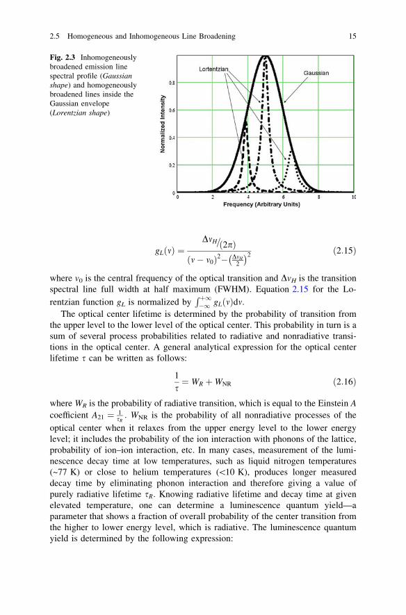
gL mð Þ ¼DmH= 2pð Þ

m� m0ð Þ2� DmH2

2 ð2:15Þ

where v0 is the central frequency of the optical transition and DvH is the transitionspectral line full width at half maximum (FWHM). Equation 2.15 for the Lo-

rentzian function gL is normalized byRþ1�1 gLðmÞdm:

The optical center lifetime is determined by the probability of transition fromthe upper level to the lower level of the optical center. This probability in turn is asum of several process probabilities related to radiative and nonradiative transi-tions in the optical center. A general analytical expression for the optical centerlifetime s can be written as follows:

1s¼ WR þWNR ð2:16Þ

where WR is the probability of radiative transition, which is equal to the Einstein Acoefficient A21 ¼ 1

sR: WNR is the probability of all nonradiative processes of the

optical center when it relaxes from the upper energy level to the lower energylevel; it includes the probability of the ion interaction with phonons of the lattice,probability of ion–ion interaction, etc. In many cases, measurement of the lumi-nescence decay time at low temperatures, such as liquid nitrogen temperatures(~77 K) or close to helium temperatures (\10 K), produces longer measureddecay time by eliminating phonon interaction and therefore giving a value ofpurely radiative lifetime sR: Knowing radiative lifetime and decay time at givenelevated temperature, one can determine a luminescence quantum yield—aparameter that shows a fraction of overall probability of the center transition fromthe higher to lower energy level, which is radiative. The luminescence quantumyield is determined by the following expression:

Fig. 2.3 Inhomogeneouslybroadened emission linespectral profile (Gaussianshape) and homogeneouslybroadened lines inside theGaussian envelope(Lorentzian shape)

2.5 Homogeneous and Inhomogeneous Line Broadening 15

gLQE ¼WR

WR þWNRð2:17Þ

Typical values of the room temperature luminescence decay in rare earth ions insolids (which is a result of the radiative and nonradiative transitions occurring inthese optical centers) span from microseconds to milliseconds and are dependenton the particular ion and the host material. For example, in glass at room tem-perature, the lifetime of Yb3+ and Er3+ ions in their most important laser transitionsare typically 1 and 10 ms, respectively.

Because of the higher phonon energy in silica glass than in phosphate glass, theprobability of a nonradiative transition for a given gap between higher and lowerenergy levels is higher in silica glass because it requires a smaller number ofparticipating phonons to fill the gap during relaxation from the upper level; thisdemonstrates the influence of the host material (energy gap law will be describedin detail later in the book). In turn, this fact explains why homogeneous broadeningin silica glass is usually greater than in phosphate glass. At low levels of doping,the ion–ion interaction between rare earth ions is very low; nonradiative transitionprobabilities originate mostly from electron exchange with lattice phonons.However, with an increase of the doping level, ion–ion interaction becomes moreand more significant and may result in concentration quenching of luminescence,which affects the optical center luminescence quantum yield. In turn, this sets alimit for doping concentration levels in fibers and laser hosts in general. Otherfactors may also affect the decision to limit concentration of the laser-active ions ata certain concentration level.

2.5.2 Inhomogeneous Broadening

Inhomogeneous broadening of the optical center’s line shape during a transitionbetween energy levels originates from a local site-to-site variation in the opticalcenter’s surrounding field in the lattice environment. The strength and symmetryof the field around the rare earth ion determine the spectral properties of the opticaltransitions, as well as the transition strength. In the case of inhomogeneousbroadening, the overall shape of the spectral line is a superposition of all indi-vidual, homogenously broadened lines corresponding to different types of theoptical center. The line shape of the inhomogeneously broadened optical transitionis described by the Gaussian line profile (see Fig. 2.3), which can be expressed asthe following function of frequency:

gG mð Þ ¼ 1DmINH

ffiffiffiffiffiffiffiffiffi

4ln2p

r

exp �4ln2m� m0

DmINH

� �2" #

ð2:18Þ

16 2 Optical Properties and Optical Spectroscopy of Rare Earth Ions in Solids

where DvINH is the FWHM of the inhomogeneously broadened line. Determinedby the optical center surrounding fields, the inhomogeneous line width is insen-sitive to the temperature of the host material.

In a real situation at room temperature, the individual contribution to the opticaltransition overall line shape by homogeneous and inhomogeneous broadening maybe different or even comparable, such as in the case of most rare earth ions inglasses. In this general case, the resultant overall line shape is best described by theso-called Voigt function, which is a convolution between Lorentzian and Gaussianprofiles:

gVOIGT mð Þ ¼Z

gG nð ÞgL m� nð Þdn

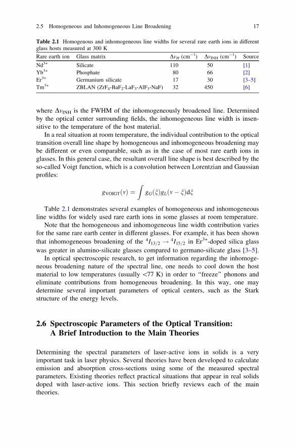
Table 2.1 demonstrates several examples of homogeneous and inhomogeneousline widths for widely used rare earth ions in some glasses at room temperature.

Note that the homogeneous and inhomogeneous line width contribution variesfor the same rare earth center in different glasses. For example, it has been shownthat inhomogeneous broadening of the 4I13=2 ! 4I15=2 in Er3+-doped silica glasswas greater in alumino-silicate glasses compared to germano-silicate glass [3–5].

In optical spectroscopic research, to get information regarding the inhomoge-neous broadening nature of the spectral line, one needs to cool down the hostmaterial to low temperatures (usually \77 K) in order to ‘‘freeze’’ phonons andeliminate contributions from homogeneous broadening. In this way, one maydetermine several important parameters of optical centers, such as the Starkstructure of the energy levels.

2.6 Spectroscopic Parameters of the Optical Transition:A Brief Introduction to the Main Theories

Determining the spectral parameters of laser-active ions in solids is a veryimportant task in laser physics. Several theories have been developed to calculateemission and absorption cross-sections using some of the measured spectralparameters. Existing theories reflect practical situations that appear in real solidsdoped with laser-active ions. This section briefly reviews each of the maintheories.

Table 2.1 Homogenous and inhomogeneous line widths for several rare earth ions in differentglass hosts measured at 300 K

Rare earth ion Glass matrix DvH (cm-1) DvINH (cm-1) Source

Nd3+ Silicate 110 50 [1]Yb3+ Phosphate 80 66 [2]Er3+ Germanium silicate 17 30 [3–5]Tm3+ ZBLAN (ZrF4-BaF2-LaF3-AlF3-NaF) 32 450 [6]

2.5 Homogeneous and Inhomogeneous Line Broadening 17

2.6.1 Judd-Ofelt Theory

The Judd-Ofelt theory [7, 8] allows one to predict the stimulated emission cross-section peaks and integrated values for transitions between any level of the ion. Thetheory is based on the assumption that the average energy difference between the 4flevels is much larger than the energy spread of the excited configuration. Theradiative transition rates and the radiative lifetimes can be obtained from theoscillator strengths of the transition. The theory gives the following expression forthe oscillator strength of the electric dipole transition (f ed) [7]:

f edij ¼

8p2mm3hð2J þ 1Þ �

n2 þ 2ð Þ2

9n�X

k¼2;4;6

Xk f NJ�

�

� Ukj j f NJ0�

�

�

�

�

�

�

�

2 ð2:19Þ

where i is the initial state of the transition, j is the final state of the transition, v is thetransition frequency, n is the refractive index of the host material, m is the electronmass, and f NJh j Ukj j f NJ0j i are the reduced matrix elements, tabulated in [9].

Within this theory, the strength of any transition f can be determined by a set ofthree parameters: Xi (i = 2, 4, 6; see Eq. 2.19 for the oscillator strength). This setof parameters completely defines and parameterizes the effect of the host on theabsorption and fluorescence properties of the ion’s transitions between differentmultiplets of the 4f N configuration. These parameters are calculated by performinga least-squares fit of the measured oscillator strengths to the theoretical ones. Themore transitions that are taken into account during the fitting procedure, the moreaccurately determined and reliable the Judd-Ofelt coefficients appear to be(although this is not the case for Yb3+, where the only transition between essen-tially two levels is presented in the electronic structure of the ion; see below). Thecomplete set of Judd-Ofelt coefficients allows the calculation of the strength of anyintegrated cross-section. Judd-Ofelt parameters are presently tabulated for prac-tically all rare earth ions in different solid materials. Table 2.2 presents the Judd-Ofelt parameters for Er3+ in different glass hosts (a detailed spectroscopic analysisof this ion will be done in Chap. 5).

For glasses, the calculated Judd-Ofelt parameters are average values of theparameters for each given site of the Er3+ ion because there is great variation of thesites that can be occupied by the ion (compared with crystals).

The Judd-Ofelt theory gives the total oscillator strength for the transitionbetween two multiplets. The theory estimates only the integrated electric dipoleoscillator strength for the particular transition (not the individual transitionsbetween different states of the multiplet). Determination of the individual transi-tions’ strength or cross-sections (spectral shapes) requires determination of thespectral distribution measurements of the relative emission spectra. This theory isparticularly valuable for predicting strengths of transitions for which direct mea-surements are difficult. Accuracy of the Judd-Ofelt analysis is about 10–15 % for

18 2 Optical Properties and Optical Spectroscopy of Rare Earth Ions in Solids

most rare earth ions [13, 14]. Detailed treatments of the theory for the case of rareearth ions, including its successes and limitations, are available elsewhere [12, 15].

On a practical note, for fiber laser development in which Yb3+ glass plays acentral role, it is practically impossible to perform a calculation of the Judd-Ofeltparameters and therefore calculate cross-section values using Judd-Ofelt theorybecause there is only a 2F5=2 ! 2F7=2 transition (i.e., essentially a two-leveltransition) for Yb3+. Other theoretical methods (described later) are used in thecase of Yb3+ to determine cross-section values of optical transitions.

2.6.2 McCumber Theory

In a glass environment, rare earth ions demonstrate broad emission and absorptionspectra; therefore, the previously introduced Einstein relationships need to beadjusted. For this important application, the McCumber theory can be used. TheMcCumber theory shows that all three processes described by Einstein in histheory—absorption, stimulated emission, and spontaneous decay—their cross-sections, and the radiative lifetime of an optical center in thermal equilibrium arerelated to each other at every single frequency using a set of theoretical formulas.These formulas are also sometimes called a generalized Einstein relationship.

Following McCumber [16], the theory assumes that the time required toestablish a thermal distribution within each manifold is short compared with thelifetime of the manifold. The main theoretical conclusion of the McCumber theoryis the following formula, which relates absorption and emission cross-sections at a

Table 2.2 Judd-Ofelt parameters for Er3+ in different glass hosts

Glass matrix X2 9 10-20

(cm2)X4 9 10-20

(cm2)X6 9 10-20

(cm2)Source

Germanate 6.4 0.75 0.34 [10]Phosphate 9.92 3.74 7.36 [10]Fluoride 1.54 1.13 1.19 [11]

1.47 1.51 1.69 [23]Borate 11.36 3.66 2.24 [10]Tellurite 7.84 1.37 1.14 [10]Gallium tellurite 6.46 1.64 1.47 [26]ZBLAN (ZrF4-BaF2-LaF3-AlF3-NaF) 2.3 0.9 1.7 [12]PKBAEr 8.05 1.46 2.28 [22]NaTFP 5.92 1.07 1.44 [23]Lead borate 3.31 1.63 1.29 [24]ZTE 3.14 1.19 1.43 [25]Oxyfluoride 2.75 1.25 0.76 [26]Silica 8.15 1.43 1.22 [28]

2.6 Spectroscopic Parameters of the Optical Transition 19

given frequency (unlike the Füchtbauer-Ladenburg theory, which gives the rela-tionship between integrated cross-sections):

r21ðmÞ ¼ r12ðmÞexpEex � hm

kT

� �

ð2:20Þ

where Eex is the excitation energy, which is temperature dependent and is the netfree energy required to excite an ion from its lower energy level to the upper levelat temperature T. At room temperature, kT & 161 cm-1. According to theMcCumber analysis, the emission and absorption cross-sections are equal at acertain frequency:

mcenter ¼Eex

hð2:21Þ

All one needs to know is Eex. To determine this important value followingMcCumber, another definition of this energy parameter is introduced:

N0þ

N0�¼ exp �Eex

kT

� �

ð2:22Þ

where N±0 is the population of the upper and lower levels in unpumped material at

temperature T.However, if one knows the positions and number of all Stark components in the

lower and upper energy levels, the same concentration ratio can be determined asfollows:

N0þ

N0�¼

expð�E0=kTÞ � 1þP

p

i¼2exp �Eþi=kT

� �

� �

1þP

q

j¼2exp �E�j=kT

ð2:23Þ

where q and p are the number of Stark components at the ground and excitedlevels, respectively; E0 is the energy separation between the lowest energy levelsof the two manifolds (zero-phonon energy); and E+i and E-j are the energy dif-ferences between ith and jth levels.

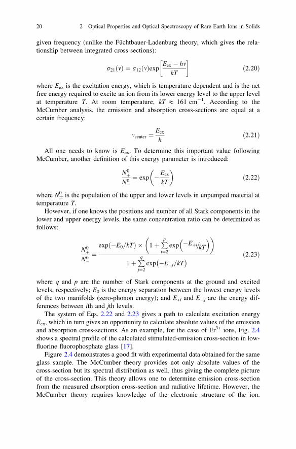
The system of Eqs. 2.22 and 2.23 gives a path to calculate excitation energyEex, which in turn gives an opportunity to calculate absolute values of the emissionand absorption cross-sections. As an example, for the case of Er3+ ions, Fig. 2.4shows a spectral profile of the calculated stimulated-emission cross-section in low-fluorine fluorophosphate glass [17].

Figure 2.4 demonstrates a good fit with experimental data obtained for the sameglass sample. The McCumber theory provides not only absolute values of thecross-section but its spectral distribution as well, thus giving the complete pictureof the cross-section. This theory allows one to determine emission cross-sectionfrom the measured absorption cross-section and radiative lifetime. However, theMcCumber theory requires knowledge of the electronic structure of the ion.

20 2 Optical Properties and Optical Spectroscopy of Rare Earth Ions in Solids

Overall, the McCumber theory is a powerful instrument in hands of researchers forcalculating important spectroscopic parameters of laser-active optical centers andis often used in laser physics.

2.6.3 Füchtbauer-Ladenburg Theory and EinsteinCoefficients

The Füchtbauer-Ladenburg theory [18, 19] provides a relationship between theabsorption coefficient and Einstein A and B coefficients for a system with twodegenerate levels, using degeneracy terms g1 and g2 for the lower and upperenergy levels. This theory assumes that in the spectral range of interest (i.e., wherethe optical transitions under consideration are taking place), the host materialrefractive index remains unchanged—an assumption that is reasonable for trivalentrare earth ions, which are being used as laser-active optical centers. The mostimportant and probably most well-known conclusion of the Füchtbauer-Ladenburgtheory is an obtained relationship between the upper-state lifetime of the laser-active ion to its emission cross-section. The corresponding Füchtbauer-Ladenburgrelationship is given by:

Z

m2r21 mð Þdm ¼ A21c2

8pn2ð2:24Þ

where n is the refractive index; A21 is the Einstein coefficient, which is determined

by radiative lifetime, A21 ¼ 1=srad; c is the speed of light in a vacuum; v is

Fig. 2.4 Comparison of theshape of the measuredstimulated-emission cross-section with that calculatedfrom the absorption cross-section using the McCumbertheory [17]. (Image courtesyof the optical Society ofAmerica)

2.6 Spectroscopic Parameters of the Optical Transition 21

frequency; and r21(v) is the spectral component of the emission cross-section.A similar equation can be written for the absorption cross-section:

Z

m2r12 mð Þdm ¼ A21c2

8pn2

g2

g1ð2:25Þ

The relationships in Eqs. 2.24 and 2.25 give a well-known relationship betweenabsorption and emission cross-sections:

g1

Z

m2r12 mð Þdm ¼ g2

Z

m2r21 mð Þdm ð2:26Þ

A comparison of the theories presented in this chapter for calculating emissioncross-sections are illustrated in Fig. 2.5 [17]. According to Fig. 2.5, the McCumbertheory shows very good agreement with measured cross-section values, whereas theEinstein analysis overestimates these values.

Another example of using the Füchtbauer-Ladenburg theory for stimulated-emission cross-section calculations is illustrated in Fig. 2.6 [20]. Dong et al. [20]determined stimulated-emission cross-sections for the 3 % Nd-doped phosphateglass at both room and liquid-nitrogen temperatures using this theory.

Figure 2.6 shows variations with temperature in the stimulated-emission cross-sections of Nd:phosphate glasses calculated using the Füchtbauer-Ladenburgtheory. The results show that the stimulated-emission cross-section is nearlyindependent of Nd3+ concentration. These results are important because depen-dence of the emission cross-section on the temperature has a significant effect onthe performance of high-power Nd:glass-based lasers.

In addition to giving a path to calculate cross-sections, the Füchtbauer-Ladenburg theory shows that large emission cross-sections and therefore a

Fig. 2.5 Comparison ofstimulated-emission cross-sections of Er3+ obtainedusing the radiative lifetime(measured), the Einsteinrelationship, and theMcCumber theory with anestimated e : Eex for thecase of fluorophosphates glass[17]. (Image courtesy of theoptical Society of America.)

22 2 Optical Properties and Optical Spectroscopy of Rare Earth Ions in Solids

large-gain bandwidth of laser transitions are leading to a short radiative lifetime.This helps researchers to determine the laser-active optical centers that are requiredfor broad-wavelength tunable laser operation and ultrashort pulse generation.

2.7 Sensitization of Laser-Active Centers

Trivalent rare earth ions used as laser-active centers in solids have several spec-troscopic properties that restrict effective optical excitation for creating inversionpopulations. The most important spectroscopic properties that have been taken intoaccount during rare-earth-doped gain fiber development for laser/amplifier appli-cations are spectral line width, accessibility of the absorption band for excitingwith pump-diode laser wavelengths, and absorption coefficients at the pumpwavelength for reasonable gain of fiber length.

If only the most widely used laser-active rare earth centers in fiber lasers (i.e.,Nd3+, Yb3+, Er3+, and Tm) and their absorption bands are considered, we can seethat all ions except for Er3+ require well-developed diode laser pump wavelengthsof 808, 915, 976 and 792 nm when using common high-intensity excitation bandswith high absorption coefficients (e.g., for Liekki Yb3+ [nLIGHT, Vancouver,WA], [1,200 dB/m of core absorption). Unlike the other ions mentioned, Er3+

demonstrates intense absorption near 1,530 nm with ~70–110 dB/m absorptioncoefficient and another absorption band near 980 nm with approximately one-thirdof that at 1,530 nm absorption band intensity. On the other hand, for high-powerapplications when pump-diode lasers are fiber coupled into 100–600 lm corefibers, a technology called clad pumping has been developed to make it possible tocouple high-power diode lasers into the gain fibers (reviewed in detail later in thisbook). To use the clad pumping technique. The gain fiber consists of a doped core

Fig. 2.6 Stimulated-emission cross-sectionsversus temperature fordifferently doped glasses. Thestraight line represents themodel described in Ref. [20],which predicts the variationof the stimulated-emissioncross-section ofNd:phosphate glasses withtemperature [20, 21]. (Imagecourtesy of the opticalSociety of America.)

2.6 Spectroscopic Parameters of the Optical Transition 23

and undoped cladding where the pump is coupled. However, because of the lowratio of core to clad diameter, the effective absorption of the pump light is reducedfrom the core absorption coefficient to the value:

aclad ¼ acoreScore

Scladð2:27Þ

where Score and Sclad are cross-section areas of the core and cladding, respectively.For typical true single-mode fibers with a core diameter of 9 lm and clad diameterof 125 lm, the cross-section area ratio is 0.005. Therefore, the clad pumpingabsorption coefficient reduces from 110 to 0.55 dB/m, which in turn requires anincrease of the fiber length by a factor of 200.

One of the well-known techniques that is used to increase absorption of laser-active ions and enhance efficiency of rare-earth ion excitation is co-doping thelaser active ion with another ion, using a more suitable pumping spectral location,a high doping concentration, and an efficient pumping excitation transfer to thelasing ion. Therefore, this technique is very important in clad pumping geometryin which, as mentioned above, effective absorption of the active laser center in thecladding is reduced significantly. As an example, in the case of Er3+, it wassuggested that Yb3+, which has an intense and broad absorption band at 980 nm,can be a very good sensitizer. Experimental and theoretical research of the energytransfer between Yb3+ and Er3+ in different materials showed that direct excitationof Yb3+ produces a very efficient energy transfer to Er3+ in several laser glass hosts(see Fig. 2.7). In the case of the Yb3+–Er3+ system, Yb3+ ions absorb pumpinglight in their broad absorption band at 980 nm, which follows an efficient energytransfer from the 2F5=2 level of Yb3+ to the 4I11=2 level of Er3+. This is followed byfast nonradiative relaxation from the 4I11=2 energy level to the metastable 4I13=2

energy level. The 4I13=2 energy level is an upper energy level of the 1,550 nm Er3+

fiber laser (see Fig. 2.7).Concentration of Yb3+ is usually much higher than the concentration of Er3+ in

such co-doped systems, which make pump absorption higher and give reasonablegain fiber lengths in case of clad-pumping geometry. In addition, 980 nm indiumgallium arsenide (InGaAs) laser diodes are available with higher power models

Fig. 2.7 Simplifiedexcitation and energy transferprocess in an Er3+-dopedglass sensitized with Yb3+

24 2 Optical Properties and Optical Spectroscopy of Rare Earth Ions in Solids

and demonstrate much higher electrical to optical efficiency ([60 %) compared to~25–30 % for 1,470–1,530 nm diode lasers used for direct Er3+ excitation. Unlikethe case of Yb3+ sensitization, however, where there is a big quantum defectbetween pump and lasing photon energies, Er3+ fiber lasers with direct (i.e., res-onant) excitation in the 1,450–1,550 nm spectral range may demonstrate highfiber-laser energy efficiency, high slope efficiency, and low quantum defects,which in turn reduce the heat generated by the laser medium. For high-power Er3+-doped fiber laser systems, such resonant excitation plays a crucial role in solvingthe problem of thermal management of the laser system. However, when thisapproach is applied to clad pumping geometry, it requires achievement of highlaser-active Er3+ concentration in laser glass with absent of luminescencequenching, which in turn is a challenging task. Because of the quasi-three-energylevel (i.e., resonant nature) of the direct excitation of Er3+ when pumped directlyinto the 1,450–1,530 nm band, this approach requires higher pump power densitiesto reach transparency of the resonant Er3+ absorption in order to eliminatereabsorption of signal power and achieve positive net gain.

References

1. J.M. Pellegrino, W.M. Yen, M.J. Weber, Composition dependence of Nd3+ homogeneous linewidths in glasses. J. Appl. Phys. 51, 6332 (1980)

2. J.T. Fournier, R.H. Bartram, Inhomogeneous broadening of the optical spectra of Yb3+ inphosphate glass. J. Phys. Chem. Solids 31, 2615–2624 (1970)

3. R.I. Laming, L. Reekie, P.R. Morkel, D.N. Payne, Multichannel cross talk and pump noisecharacterization of Er3+ doped fiber amplifiers pumped at 980 nm. Electron Lett. 25, 455–456(1989)

4. E. Desurvire, J.L. Zyskind, J.R. Simpson, Spectral gain hole-burning at 1.53 um in erbium-doped fiber amplifiers. IEEE Photon. Technol. Lett. 2(4), 246–248 (1990)

5. J.L. Zyskind, E. Desurvive, J.W. Sulho, D. DiGiovanni, Determination of homogeneous linewidth by spectral gain hole-burning in an erbium-doped fiber amplifier with a GeO2-SiO2core. IEEE Photon. Technol. Lett. 2(12), 869–871 (1990)

6. F. Roy, D. Bayart, C. Heerdt, A.L. Sauze, P. Baniel, Spectral hole burning measurementthulium-doped fiber amplifiers. Opt. Lett. 27(1), 10–12 (2002)

7. B.R. Judd, Optical absorption intensities of rare-earth ions. Phys. Rev. 127, 750–761 (1962)8. G.S. Ofelt, Intensities of crystal spectra of rare-earth ions. J. Chem. Phys. 37, 511–520 (1962)9. C.W. Nielson, G.F. Koster, Spectroscopic Coefficients for the pn; dn and f n Configurations

(MIT Press, Cambridge, MA, 1963)10. R. Reisfeld, in Spectroscopy of Solid-State Laser-Type Materials, ed. by B.D. Bartolo

(Plenum Press, New York, 1987), pp. 343–39611. R. Reisfeld, G. Katz, N. Spector, C.K. Jorgensen, C. Jacohoni, R. de Pape, J. Sol. St. Chem.

41, 253 (1982)12. F. Auzel, Risita della statz. Sper. Vetro 5, 49 (1990)13. M.J. Weber, T.E. Varitimos, B.H. Matsinger, Optical intensities of rare-earth ions in yttrium

orthoaluminate. Phys. Rev. B 8, 47 (1973)14. W.J. Miniscalco, Rare Earth Doped Fiber Lasers and Amplifiers (Marcel Dekker, Inc., New

York, 1993), p. 33

2.7 Sensitization of Laser-Active Centers 25

15. C. Gorrller-Walrand, K. Binnemans, Handbook on the Physics and Chemistry of Rare Earths,vol. 25 (Elsevier Science, 1998), p. 167

16. D.E. McCumber, Theory of phonon-terminated optical lasers. Phys. Rev. 134(2A), A299–A306 (1964)

17. W.J. Miniscalco, R.S. Quimby, General procedure for the analysis of Er3+ cross sections.Opt. Lett. 16(4), 258–260 (1991)

18. P.H. Sarkies, J.N. Sandoe, S. Parke, Variations of Nd3+ cross section for stimulated emissionwith glass composition. J. Phys. D: Appl. Phys. 4(10), 1642–1649 (1971)

19. J.N. Sandoe, P.H. Sarkies, S. Parke, Variation of Er3+ cross section for stimulated emissionwith glass composition. J. Phys. D: Appl. Phys. 5, 1788–1799 (1972)

20. J. Dong, M. Bass, C. Walters, Temperature-dependent stimulated-emission cross section andconcentration quenching in Nd3+-doped phosphate glasses. J. Opt. Soc. Am. B 21, 454–457(2004)

21. A. C. Erlandson, G. F. Albrecht, S. E. Stokowski, Model predicting the temperaturedependence of the gain coefficient and the extractable stored energy density in Nd:phosphateglass lasers. J. Opt. Soc. Am. B 9, 214–222 (1992).

22. P. Babu, H.J. Seo, K.H. Jang, R. Balakrishnaiah, C.K. Jayasankar, K.-S. Lim, V. Lavín,Optical spectroscopy, 1.5 lm emission, and upconversion properties of Er3+-dopedmetaphosphate laser glasses. J. Opt. Soc. Am. B 24, 2218–2228 (2007)

23. M. Jayasimhadri, L.R. Moorthy, K. Kojima, K. Yamamoto, N. Wada, Er-dopedtellurofluorophosphate glasses for lasers and optical amplifiers. J. Phys. Condens. Matter.17, 7705–7717 (2005)

24. W.A. Pisarski, Spectroscopic analysis of praseodymium and erbium ions in heavy metalfluoride and oxide glasses. J. Mol. Struct. 744–747, 473–479 (2005)

25. C. Laxmi kanth, B.V. Ragavaiah, B. Appa Rao, N. Veeraiah, Optical absorption, fluorescenceand thermoluminescence properties of ZnF2-MO-TeO2 (MO = ZnO, CdO and PbO) glassesdoped with Er ions. J. Lumin 109, 193–205 (2004)

26. X. Qiao, X. Fan, M. Wang, X. Zhang, Up-conversion luminescence and near infraredluminescence of Er3+ in transparent oxyfluoride glass-ceramics. Opt. Mater. 27, 597–603(2004)

27. H. Lin, K. Liu, E.Y.B. Pun, T.C. Ma, X. Peng, Q.D. An, J.Y. Yu, S.B. Jiang, Infrared andvisible fluorescence in Er-doped gallium tellurite glasses. Chem. Phys. Lett. 398, 146–150(2004)

28. D. Ning, Y. Iv-yun, P. Ming-ying, Z. Qing-ling, C. Dan-ping, T. Akai, K. Kadono,Preparation and spectroscopic properties of Er3+-doped high silica glass by sinteringnanoporous glass. Mater. Lett. 60, 1987–1989 (2006)

26 2 Optical Properties and Optical Spectroscopy of Rare Earth Ions in Solids

Chapter 3Physical and Optical Properties of LaserGlass

Glass is an amorphic material that is highly isotropic and demonstrates a highdegree of homogeneity. Unlike crystals, glass molecules are disordered but arerigidly bound. The structure of the glass shows bounds of several molecules:matrix molecules such as (SiO4)4- or (PO4)3- for silicate or phosphate glasses,respectively, and molecules of different metals or other chemical elements (usuallytheir oxides). Optical properties of optically clear glass, particularly laser glass, arecharacterized by the spectrally dependent refractive index n = f (k). For most laserglasses, the value of the refractive index in the vicinity of a 1 lm wavelength isclose to 1.5. This value depends on the particular laser glass structure and dopingof the material. Table 3.1 demonstrates several examples of the glass compositionfor several of the most commonly used laser glasses.

An important characteristic of the host material for a gain medium is itsprincipal optical phonon energy. Large phonon energy is associated with shortcarrier lifetimes arising from a large nonradiative relaxation rate. The phonons thatare participating in the nonradiative relaxation process are the highest energyphonons in the phonon spectrum of the host material, which have a big value ofdensity of states. There active phonons that are responsible for nonradiativerelaxation are called effective phonons, with individual phonon energy equal tohX. If the number of effective phonons involved in the multiphonon relaxationprocess is designated as p, then the corresponding energy gap DE can be expressedby effective phonon energy as follows:

p ¼ DE

�hXð3:1Þ

The so-called energy gap law is:

Wnr ¼ Anr � exp �v� �hX� p½ � ð3:2Þ

where Anr and v are constant parameters of the host material and �h is the reducedPlanck constant. Parameter Anr is inversely proportional to the characteristicnonradiative decay time s0, while constant v is related to the details of the

V. Ter-Mikirtychev, Fundamentals of Fiber Lasers and Fiber Amplifiers,Springer Series in Optical Sciences 181, DOI: 10.1007/978-3-319-02338-0_3,� Springer International Publishing Switzerland 2014

27

electron–phonon coupling and is a function of phonon energy and the electron–phonon coupling constant:

v ¼ ln eð Þ�hX

ð3:3Þ

where e � 1 is the ratio of the multiphonon relaxation rate for a p-phonon processto that for a (p - 1) phonon process [2]. In glasses, the value of parameter e is inthe range between 0.012 and 0.007, which is less than the value of the sameparameter in crystals. This fact motivates some researchers to conclude that thatthe strength of electron–phonon coupling in glasses is weaker than that in crystals.In general, if one considers same value of the energy gap, the probability ofmultiphonon nonradiative decay in glasses is higher compared with that in crys-tals, which in turn can be explained by a bigger span of available phonons withdifferent energies in the phonon spectrum of glasses.

It is important to note that this simple form of the energy gap law (i.e., non-radiative rate law) is only valid for rare earth (RE3+) ions that demonstrate the caseof weak electron–phonon coupling with a Huang-Rhys parameter S close to zero.

As you can see from this analysis, the nonradiative relaxation rate is a verystrong function of the lasing transition energy (the gap) to phonon energy ratio:The higher this ratio, the lower is the probability of nonradiative relaxation fromlaser-active level because more phonons have to be involved into the relaxationprocess between separated energy levels. Note that nonradiative relaxation fromthe upper energy level of the laser transition reduces the luminescence quantumyield of the optical center and therefore is critical for laser efficiency. Therefore,host materials with low phonon energies are required, especially for infrared (IR)laser materials with relatively small lasing photon energy.

3.1 Mechanical and Thermal Properties of Glass

This section briefly reviews the main thermomechanical properties of fiber glassand compares them to that of crystalline materials used for laser applications. As inthe case of volume glass, the following advantageous properties of the glass can bedefined, which make a difference in optical fibers:

Table 3.1 Composition of several commonly used optical fiber glasses [1] (Courtesy of theOptical Society of America)

Glass Composition (mol. %)

Phosphate 50(P2O5)–16.66(MgO)–33.34(Li2O)Germanate 66(GeO2)–17(BaO)–17(K2O)Tellurite 80(TeO2)–20(Li2O)ZBLAN 57.35(ZrF4)–29.63(BaF2)–3.54(LaF3)

-1.78(NaF)–5.16(InF3)–2.54(AlF3)

28 3 Physical and Optical Properties of Laser Glass

1. High degree of optical uniformity over a long length.2. Susceptibility of the glass matrix to change its nonlinear, mechanical, thermal,

and spectral parameters by appropriate doping of the glass matrix in wide rangeof doping levels.

3. Possibility of achieving required photosensitivity to the ultraviolet (UV) light inthe laser-active fiber for fiber grating recording.

4. Manufacturing optical fibers of long length with cost-effective production lines.5. Relatively easy ways of connecting different pieces of fibers with low con-

nection loss (using commercially available splicing machines).

When one cools down the glass that is in liquid phase (after melting), thetemperature point that corresponds to the transition from a liquid to a brittle glasscondition is called the glass transition temperature, Tg. The same temperature isresponsible for the transition from solid to soft phase during the heating process.More accurately, the glass transition temperature is responsible for the so-calledphase transition in glass, in which a super-cooled melt during cooling becomes aglassy structure. Below Tg, an amorphous glass is in a solid glass state and internalglass structure is mostly restored. During cooling from the liquid phase, the glasstransition is a result of increased viscosity, which in turn depends on the coolingrate. During slow cooling, there is enough time for the glass liquid to restore itslocal atomic structure, whereas during rapid cooling, this process results in anincrease in viscosity. Local atomic structure is not restored, which in turn results inan increase of the transition temperature Tg. Rapid and slow cooling result indifferent glass structures. These circumstances are taken into account in the glassmanufacturing process. Tg plays an important role in high-power fiber laser designbecause it determines the upper limit of the allowed local temperatures of the fibercomponents, as well as that of gain fibers.

Table 3.2 highlights some of the most important thermomechanical propertiesof glass in comparison with yttrium aluminium garnet (YAG) crystal, which iswidely used in laser physics (host of Nd:YAG laser material).

It is also useful here to present data on material density for several of the mostpopular glasses used in fiber laser technology (see Table 3.3).

Table 3.2 Thermomechanical properties of yttrium aluminium garnet (YAG) crystal and glass(fused silica)

Parameter YAG crystal Glass (fused silica)

Refractive index at 1,000 nm 1.83 1.47Thermal conductivity, W/(m K) 14 0.3–1.3dn/dT (10-6/K-1) 9.8 -20 to +10Hardness (Moh) 8.5 7Linear coefficient of thermal expansion (10-5/K) 0.8-0.9 0.5Melting point, �C (for glass: transition temperature Tg) 1,970 500a

Density (g/cm3) 4.57 2.5

a Transition point temperature is listed. Melting point is ~1,600 �C

3.1 Mechanical and Thermal Properties of Glass 29

Crystalline solid-state laser materials such as YAG are superior to glasses inthermal conductivity and mechanical strength. Glasses, because of the extremelylarge lengths of material used when making use of distributed heat along theirsurface, create great opportunities for solving many thermal management issuesexisting in crystalline lasers. In addition, some spectroscopic parameters of thelaser glass, such as broad absorption lines, make them superior for many diodepump applications (reviewed in later chapters).

3.2 Optical Properties of Fibers (Attenuation)

Because attenuation plays a very important role in the light propagation charac-teristics of fiber, this section provides a brief review of factors affecting thisphysical parameter of the glass. The physical reasons that are responsible forattenuation in optical fibers can be divided into three main categories: intrinsicglass material properties, waveguide properties, and optical connection loss.

3.2.1 Intrinsic Glass Material Properties

Intrinsic glass attenuation arises from absorption and scattering. Like in crystals,optical transmission properties of the glass reflect the degree of material purity andthe method of its manufacture.

Fiber attenuation is caused by bonds between hydrogen atoms and oxygen inthe glass material. The hydrogen atoms attach to oxygen sites and form hydroxylions. These oxygen and fundamental vibration bands are the most important andcommon impurities in undoped (laser-inactive) glasses, which in turn determinethe UV cutoff and the presence or absence of bands in the vicinity of 250, 1,400,and 2,700 nm. The IR edge is between 4.5 and 5.0 lm, corresponding to funda-mental inter zone optical transitions. Because of the great variety of glass com-position used for different fibers, no single glass composition provides continuoustransparency from the visible spectral region through the mid-infrared spectralregion. Note that intentionally introduced dopants, such as GeO2 and P2O5, whichmodify the fiber refractive index profile and change the manufacturing process,also affect material attenuation.

Table 3.3 Material densityof several glasses [3]

Glasses Density (g/cm3)

Silicate 2.5–2.7Borate 2.4–2.5Phosphate ~2.6Fluoride ~6–7

30 3 Physical and Optical Properties of Laser Glass

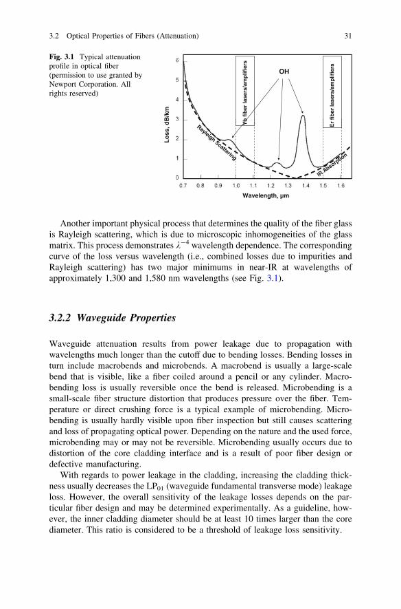
Another important physical process that determines the quality of the fiber glassis Rayleigh scattering, which is due to microscopic inhomogeneities of the glassmatrix. This process demonstrates k-4 wavelength dependence. The correspondingcurve of the loss versus wavelength (i.e., combined losses due to impurities andRayleigh scattering) has two major minimums in near-IR at wavelengths ofapproximately 1,300 and 1,580 nm wavelengths (see Fig. 3.1).

3.2.2 Waveguide Properties

Waveguide attenuation results from power leakage due to propagation withwavelengths much longer than the cutoff due to bending losses. Bending losses inturn include macrobends and microbends. A macrobend is usually a large-scalebend that is visible, like a fiber coiled around a pencil or any cylinder. Macro-bending loss is usually reversible once the bend is released. Microbending is asmall-scale fiber structure distortion that produces pressure over the fiber. Tem-perature or direct crushing force is a typical example of microbending. Micro-bending is usually hardly visible upon fiber inspection but still causes scatteringand loss of propagating optical power. Depending on the nature and the used force,microbending may or may not be reversible. Microbending usually occurs due todistortion of the core cladding interface and is a result of poor fiber design ordefective manufacturing.

With regards to power leakage in the cladding, increasing the cladding thick-ness usually decreases the LP01 (waveguide fundamental transverse mode) leakageloss. However, the overall sensitivity of the leakage losses depends on the par-ticular fiber design and may be determined experimentally. As a guideline, how-ever, the inner cladding diameter should be at least 10 times larger than the corediameter. This ratio is considered to be a threshold of leakage loss sensitivity.

Yb

fib

er la

sers

/am

plif

iers

Er

fib

er la

sers

/am

plif

iers

OH

Rayleigh Scattering

IR Absorption

Wavelength, µm

Lo

ss, d

B/k

m

Fig. 3.1 Typical attenuationprofile in optical fiber(permission to use granted byNewport Corporation. Allrights reserved)

3.2 Optical Properties of Fibers (Attenuation) 31

A detailed description of waveguide properties (i.e., fiber mode structure) iscovered in Chap. 6.

3.2.3 Optical Connection Loss

Two pieces of fiber spliced together demonstrate so-called joint losses. Currently,the commercially available splicing machines demonstrate down to 0.01–0.02 dBsplicing loss for identical fibers. If there is mode field diameter mismatch forsingle-mode fibers, the optical connection (splicing) loss can be calculated usingfollowing formula:

Lcl ¼ �20 log2w1w2

w21 þ w2

2

� �

ð3:4Þ

where w1 and w2 are mode field radii of the two spliced fibers. The mode fieldradius is defined as half of the spatial extend of the fundamental mode through alarger volume, including the inner fiber cladding, where the mode intensity dropsto the level of 1/e2.

3.3 Different Glass Types Used in Fiber Lasersand Amplifiers

Glasses differ by their principal phonon energy, which in turn affects the proba-bility of nonradiative relaxation in these glasses. Nonradiative relaxation plays animportant role in laser efficiency and therefore is a crucial parameter of the solid-state gain material.

Different chemical compounds added to the glass matrix—such as germanium,phosphorus, borate, and tellurite—can be used to create germinate, phosphate,borate, and tellurite glasses, respectively. Currently, the most widely used mate-rials for fiber laser applications are silicate, germano-silicate, tellurite, and phos-phate glasses doped with rare earth laser-active ions. Table 3.4 shows the principal

Table 3.4 Principal phononenergies in the most widelyused laser glasses [4–6]

Glass system Phonon energy (�hX, 1/cm)

Borate 1,400Phosphate 1,200Silicate 1,100Germanate 900Tellurite 700Fluorozirconate 500Chalcogenide 350

32 3 Physical and Optical Properties of Laser Glass

phonon energies for the most widely used glasses [4–6]. Borate glass demonstratesthe highest phonon energy, whereas chalcogenide glass shows the lowest phononenergy. The following sections briefly review several examples of importantglasses used in fiber laser development.

3.3.1 Silicate Glass

Silica-based optical fibers are composed primarily of silicon dioxide (SiO2) andcertain amounts of other chemicals that are added for different applications.Currently, liquid silicon tetrachloride (SiCl4) in a gaseous stream of pure oxygen isthe principal source of silicon for the vapor deposition method (which will bereviewed later). Glass medium modifiers, such as Na3+ and Al3+, are often added tofacilitate the incorporation of rare earth ions because their size is greater than thebasic network positions. The main purpose of the modifying impurities is to breakthe bridging oxygen to form non-bridging oxygen, which can later be used tocoordinate the rare earth ions. The most effective glass modifier studied in silicaglass is aluminum because it shows the most favorable characteristics. Theincorporation of 2.87 mol % of Al2O3 in Nd3+-doped silica glass has been shownto lead to elimination of Nd3+ clustering [7]. In the case of Er3+, aluminum co-doping improves the efficiency of Er3+-doped fiber amplifiers by eliminating thequenching effects [8].

Silica-based fibers have several advantages over other glass types used in fibermanufacturing. One of the main properties of the silicate glass is its manufactu-rability, which allows one to obtain high-quality fibers of long length. The nextproperty that distinguishes this fiber type is the wide range of optical transparency,thus permitting the lowest loss for optical communication. Silicate fibers aremechanically robust, demonstrating impressive tolerance to bending. Silicate glassis not hydroscopic (i.e., highly resistive to water absorption) and demonstrates ahigh degree of chemical resistance, which makes it an irreplaceable candidate formany applications where a chemically aggressive environment is present. Thesefibers have very high damage thresholds and relatively low optical nonlinearity.Probably the most serious disadvantage of the silicate glass is its high phononenergy of ~1,100 cm-1, which has to be taken into consideration when nonradi-ative multiphonon relaxation challenges development of gain fibers.

From all glass matrixes used for fiber laser applications, silicate glasses areprobably the most widely used. They are used in several high-power fiber laserapplications and currently are commercially available from a number ofcompanies.

3.3 Different Glass Types Used in Fiber Lasers and Amplifiers 33

3.3.2 Phosphate Glass

Phosphate glasses have advantages over silicate glasses in the entire set ofparameters important for laser applications. The most important advantage, par-ticularly for fiber laser applications, is that phosphate glasses allow a significantamount of doping of laser-active ions to be introduced into the glass matrix withno substantial reduction of the luminescence quantum yield. Also, phosphateglasses are stable against the action of UV radiation but have poor chemicaldurability. Only mechanical strength and thermal stability make phosphate glassinferior to silicate glass. The principal phonon energy in most phosphate glasses is~1,100–1,300 cm-1. However, the ability to be doped with a significantly higherconcentration of laser-active ions promotes the usage of phosphate glass in highpeak power, pulse lasers, and short-cavity distributed feedback fiber lasers.

3.3.3 Tellurite Glass

Tellurite glasses are the focus of a growing number of studies due to their reducedphonon energy (principal phonon energy is ~700 cm-1) and high linear andnonlinear refractive index. Tellurite glasses demonstrate good mechanical stabilityand quite wide optical transmission, ranging from 400 to 6,000 nm. Table 3.5provides the typical intrinsic loss parameters of tellurite glass.

3.3.4 Fluoride Glass and ZBLAN

ZBLAN is an abbreviation of fluorozirconate glass system composition (ZrFM4-BaF2-LaF3-AlF3-NaF) and is the basis of most fluoride fibers. It is one of manyfluoride glass compositions used to make fluoride glass and fiber. The principalphonon energy in typical fluoride glass is ~500–600 cm-1. The properties of

Table 3.5 Intrinsic loss parameters in tellurite glass [9]

UV absorption AUV = 10 9 106 dB/kmkUV = 13.0 ± 0.3 lm

Rayleigh scattering R = 0.29 dB/km (Ref. [12])IR absorption AIR = 1,000 dB/km

kIR = 4.1 lmMinimum loss (5.0 ± 0.2) 9 10-3 dB/kmMinimum loss wavelength 2.8 ± 0.1 lmLoss at 1.5 lm 0.06 dB/km

AUV and AIR are the ultraviolet (UV) and infrared (IR) absorption coefficients at correspondingwavelengths of kUV and kIR, respectively. Courtesy of the Optical Society of America

34 3 Physical and Optical Properties of Laser Glass

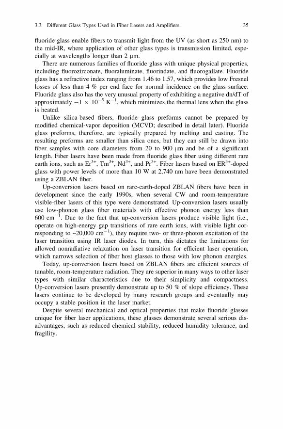
fluoride glass enable fibers to transmit light from the UV (as short as 250 nm) tothe mid-IR, where application of other glass types is transmission limited, espe-cially at wavelengths longer than 2 lm.

There are numerous families of fluoride glass with unique physical properties,including fluorozirconate, fluoraluminate, fluorindate, and fluorogallate. Fluorideglass has a refractive index ranging from 1.46 to 1.57, which provides low Fresnellosses of less than 4 % per end face for normal incidence on the glass surface.Fluoride glass also has the very unusual property of exhibiting a negative dn/dT ofapproximately -1 9 10-5 K-1, which minimizes the thermal lens when the glassis heated.

Unlike silica-based fibers, fluoride glass preforms cannot be prepared bymodified chemical-vapor deposition (MCVD; described in detail later). Fluorideglass preforms, therefore, are typically prepared by melting and casting. Theresulting preforms are smaller than silica ones, but they can still be drawn intofiber samples with core diameters from 20 to 900 lm and be of a significantlength. Fiber lasers have been made from fluoride glass fiber using different rareearth ions, such as Er3+, Tm3+, Nd3+, and Pr3+. Fiber lasers based on ER3+-dopedglass with power levels of more than 10 W at 2,740 nm have been demonstratedusing a ZBLAN fiber.

Up-conversion lasers based on rare-earth-doped ZBLAN fibers have been indevelopment since the early 1990s, when several CW and room-temperaturevisible-fiber lasers of this type were demonstrated. Up-conversion lasers usuallyuse low-phonon glass fiber materials with effective phonon energy less than600 cm-1. Due to the fact that up-conversion lasers produce visible light (i.e.,operate on high-energy gap transitions of rare earth ions, with visible light cor-responding to ~20,000 cm-1), they require two- or three-photon excitation of thelaser transition using IR laser diodes. In turn, this dictates the limitations forallowed nonradiative relaxation on laser transition for efficient laser operation,which narrows selection of fiber host glasses to those with low phonon energies.

Today, up-conversion lasers based on ZBLAN fibers are efficient sources oftunable, room-temperature radiation. They are superior in many ways to other lasertypes with similar characteristics due to their simplicity and compactness.Up-conversion lasers presently demonstrate up to 50 % of slope efficiency. Theselasers continue to be developed by many research groups and eventually mayoccupy a stable position in the laser market.

Despite several mechanical and optical properties that make fluoride glassesunique for fiber laser applications, these glasses demonstrate several serious dis-advantages, such as reduced chemical stability, reduced humidity tolerance, andfragility.

3.3 Different Glass Types Used in Fiber Lasers and Amplifiers 35

References

1. F. Pellé, N. Gardant, F. Auzel, Effect of excited-state population density on nonradiativemultiphonon relaxation rates of rare-earth ions. J. Opt. Soc. Am. B 15, 667–679 (1998)

2. C.B. Layne, W.H. Lowdermilk, M.J. Weber, Multi-phonon relaxation of rare-earth ions inoxide glasses. Phys.Rev. B, 16(1), 10–20 (1977)

3. M.J. Weber, The role of lanthanides in optical materials. American Ceramic Society annualmeeting and exposition, Cincinnati, OH, USA, 1–5 May 1995, pp. 1–18

4. R. Reisfeld, Spectroscopy of Solid-State Type Laser Materials, ed. by B. DiBartolo (PlenumPress, New York, 1987), pp. 343–396

5. C.B. Layne, M.J. Weber, Multiphonon relaxation of rare-earth ions in beryllium-fluoride glass.Phys. Rev. B16, 3259–3261 (1977)

6. D. Lezal, J. Pedlikova, J. Zavadil, Chalcogenide glasses for optical and photonics applications.Calcogenide Lett. 1(1), 11–15 (2004)

7. K. Arai, H. Namikawa, K. Kumata, T. Honda, Y. Ishii, T. Handa, Aluminium or phosphorusco-doping effects on the fluorescence and structural properties of neodymium-doped silicaglass. J. Appl. Phys. 59(10), 3430–3436 (1986)

8. S.P. Craig-Ryan, J.F. Massicott, M. Wilson, B.J. Ainslie, R. Wyatt, Optical study of lowconcentration Er3+ fibers for efficient power amplifiers, in Proceeding of ECOC’90, vol. 1(OSA, Washington DC, USA, 1990), pp. 571–574

9. M. Naftaly, S. Shen, A. Jha, Tm3+-doped tellurite glass for a broadband amplifier at 1.47 lm.Appl. Opt. 39, 4979–4984 (2000)

36 3 Physical and Optical Properties of Laser Glass

Chapter 4Fiber Fabrication and High-QualityGlasses for Gain Fibers

4.1 Materials

Glass optical fibers are almost always made from silica; however, some othermaterials, such as fluorozirconate, fluoroaluminate, and chalcogenide glasses, areused for longer-wavelength infrared applications. Most glasses demonstrate arefractive index of about 1.5. Typically, the difference between core and claddingis less than 1 %.

The core of a fiber is usually doped with laser-active ions. The most widelyused laser active ions for fiber laser applications are rare earth ions such as erbium,neodymium, ytterbium, and thulium. Each of the ions has its own absorptionbands, from which one can obtain optical gain; in turn, this creates the conditionfor optical amplification and oscillation. More detailed information on spectro-scopic characteristics of the main laser active ions in fibers are given in a laterchapter.

4.2 Fabrication of Fiber Preforms

A fiber preform is a piece of glass from which a fiber waveguide may be manu-factured by pulling it into a long length using various techniques. Most fiberpreforms are fabricated by modified chemical vapor deposition (MCVD) or out-side vapor deposition (OVD), which is a modification of MCVD. These tech-niques, which allow the achievement of optical fibers with essentially reducedlosses, revolutionized long-distance optical communications.

In the MCVD process (see Fig. 4.1), a mixture of oxygen, silicon chloride(SiCl4), and other substances [e.g., germanium chloride (GeCl4), aluminum oxide(Al2O3), rare earth dopants] are passed through a rotating silica glass tube, whichis heated from the outside to about 1,600 �C with a traversing flame.

Under high temperatures, chemical reactions in the gas take place, eventuallycreating a clear glass layer through deposition. Ingredients such as SiCl4 and

V. Ter-Mikirtychev, Fundamentals of Fiber Lasers and Fiber Amplifiers,Springer Series in Optical Sciences 181, DOI: 10.1007/978-3-319-02338-0_4,� Springer International Publishing Switzerland 2014

37

GeCl4 are easily purified by distillation because they are in liquid state at roomtemperature. Near the end of the process, the gas mixture is modified to form alayer with a higher refractive index, the precursor of the fiber core. Finally, thetube is collapsed when heated to *2,000 �C. The MCVD technique allows for theachievement of extremely low losses (\0.2 dB/km) because high-purity materialsare used during deposition and all contaminations are eliminated. Because of theabsence of hydrogen, the water content of such preforms is very small, andtherefore a strong loss peak at 1.4 lm decreases. Such a small absorption in thisspectral range is critical for optical communication applications.

An alternative to MCVD is its modification, the OVD process. Using thistechnique, a doped rod of a glass with higher refractive index is inserted into aglass tube with a lower index. Deposition occurs on the outside surface of the rod(or mandrel). When deposition is completed, the rod is removed, leaving a voidthat is collapsed after heating, eventually creating a preform. The resultant preformis a glass rod of a few centimeters diameter and roughly a meter in length.

The preforms for multimode fibers, particularly large-core fibers, are oftenfabricated with plasma outside deposition (POD), in which an outer fluorine-dopedlayer with depressed refractive index (later forming the fiber cladding) is madewith a plasma torch. The core can then be made of pure silica without any dopant.The fabrication of rare-earth-doped fibers involves various special aspects,including co-doping with other ions such as Al in special concentration ratios withlaser-active ions, as well as modification of the fiber geometry (e.g., in the cases oftriple-clad fibers).

Note that preforms for photonic crystal fibers, in which a core is surrounded bysmall holes in the cladding, are fabricated basically by stacking capillary tubes orrods that are mostly made of pure silica. However, this fiber type is outside thescope of this book.

Tube

Traversing Burner

Soot Deposition

Soot Deposition

Tube

Sintered Glass Layer

Sintered Glass Layer

Gas

Mix

ture

SiCl4

GeCl4

O2

Other

Basic MCVD

Soot Formation Zone

Fig. 4.1 Schematicillustration of modifiedchemical vapor deposition(MCVD) process

38 4 Fiber Fabrication and High-Quality Glasses for Gain Fibers

4.3 Fiber Fabrication from the Preform

Most optical fibers are currently fabricated by pulling from a preform. Along itsaxis, the preform contains a region with increased refractive index, which formsthe fiber core. When heated close to the melting point in an oven at the top of thedrawing tower (Fig. 4.2), the preform allows a thin fiber to be pulled out of thebottom side of the furnace.

The fiber from a single preform can be many kilometers long. During thepulling process, the fiber diameter is held constant by automatically adjusting thepulling speed and the furnace temperature. Before the fiber is wound up, it usuallygets a polymer coating for mechanical and chemical protection. Such coatingsoften consist of two or more different layers for optimum suppression of micro-bends. The resultant fiber structure is schematically shown in Fig. 4.3.

4.4 Laser-Active Fiber Fabrication

In laser-active fibers (i.e., gain fibers), the core is doped with laser-active ions.Typical rare-earth doping ions commonly used in fiber lasers are Yb3+, Er3+, Nd3+,and Tm3+. Co-doping laser-active fiber core with other dopants can affect the core

Fig. 4.2 Schematicillustration of the fiberfabrication process from apreform. UV Ultraviolet

4.3 Fiber Fabrication from the Preform 39

refractive index as well as the solubility of the laser-active ions themselves.Therefore, although major fiber fabrication techniques described in the previoussection are widely used for the fabrication of undoped fibers, doped (i.e., gain)fibers require modified techniques to incorporate laser-active rare earth ions intothe fiber core at certain levels of doping and distribution [1]. Currently, two majortechniques are used in laser active (gain) fiber manufacturing: MCVD (and insome cases, OVD) with solution doping of solution-phase rare earth ions and directnanoparticle deposition (DND). This section reviews each of the techniques.

4.5 MCVD Technology for Rare-Earth Doped FiberProduction

For rare-earth doped fiber manufacturing techniques based on MCVD technology,one of the main problems is that the rare earth dopants in a gas reactant should bedelivered to an oxidation reaction region together with other refractive indexcontrolling dopants. However, the rare earth reactants have a reduced vaporpressure and therefore complicate such delivery via convective transport. Toovercome this issue, one may heat the source of rare earth ions to intensify theconvection.

In MCVD, one of the most commonly used techniques for heating rare earthreactants is solution doping. In solution doping, an undoped (with rare earth ions)porous silica frit (i.e., a porous layer of silica soot) is deposited on the inner side ofa silica tube (see Fig. 4.4).

The tube is then dipped into a solution containing the rare earth ion salt. Then,the solution diffuses into the porous layer. The tube is removed from the solution,dried, and sintered into a solid glass rod, which later leads to a preform.

Figure 4.5 demonstrates the importance of Al co-doping during gain fibermanufacturing [2]. Co-doping Yb3+-doped gain fiber with Al reduces backgroundloss up to 50 times and maintains this low background loss up to a Yb3+

concentration of 1020 cm-3 [2]. Adding Al2O3 achieved a minimum loss of

Fig. 4.3 Schematic diagramof the simplest fiber structure

40 4 Fiber Fabrication and High-Quality Glasses for Gain Fibers

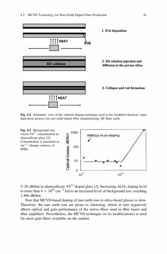
5–20 dB/km in alumosilicate Yb3+-doped glass [2]. Increasing Al2O3 doping levelto more than 4 9 1020 cm-3 led to an increased level of background loss, reaching1,400 dB/km.

Note that MCVD-based doping of rare earth ions to silica-based glasses is slow.Therefore, the rare earth ions are prone to clustering, which in turn negativelyaffects optical and gain performance of the active fibers used in fiber lasers andfiber amplifiers. Nevertheless, the MCVD technique (or its modifications) is usedfor most gain fibers available on the market.

Fig. 4.4 Schematic view of the solution doping technique used in the modified chemical vapordeposition process for rare-earth doped fiber manufacturing. RE Rare earth

Fig. 4.5 Background lossversus Yb3+ concentration inalumosilicate glass [2].Concentration is measured incm-3. (Image courtesy ofSPIE)

4.5 MCVD Technology for Rare-Earth Doped Fiber Production 41

4.6 DND Technology

For Liekki, nLight (Vancouver, WA) developed the DND technique [3]. UnlikeMCVD, DND technology directly and simultaneously (i.e., using a single step)deposits all the elements in nanoparticle size to create preforms (Fig. 4.6).

As a result, one obtains a highly doped fiber core composed of hundreds ofdeposited layers of particles with accurately controlled spatial composition. This isimportant for large mode area fibers (described in Chap. 10), which are usedwidely in high-power fiber lasers. The doping and refractive-index profile areindependently controlled, which makes it possible to achieve gain fibers withoptimized parameters.

References

1. J. Simpson, Fabrication of rare-earth doped fibers. Proc. SPIE 1171, 2–7 (1989)2. A.S. Kurkov, A.Y. Laptev, E.M. Dianov, A.N. Guryanov, V.I. karpov, V.M. Paramonov, O.I.

Medvedkov, A.A. Umnikov, V.N. protopopov, N.N. Vechkanov, S.A. Vasiliev, E.V. Pershina,Yb3+-doped double-clad fibers and lasers. Proc. SPIE 4083, 118–126 (2000)

3. S. Tammela, M. Söderlund, J. Koponen, V. Philippov, P. Stenius, The potential of directnanoparticle deposition for the next generation of optical fibers. Proc. SPIE 6116,6116.16–6116.24 (2006)

Fig. 4.6 Schematic view of the direct nanoparticle deposition technique

42 4 Fiber Fabrication and High-Quality Glasses for Gain Fibers

Chapter 5Spectroscopic Properties of Nd3+, Yb3+,Er3+, and Tm3+ Doped Fibers

5.1 Spectroscopic Notations

Rare earth (RE)3+ ion transitions show up in the optical spectrum as sharp linesthat vary little in energy position from host to host (either in glass or crystals). Thecorresponding energy level positions are designated by the following spectro-scopic notations:

2Sþ1LJ ð5:1Þ

where (2S ? 1) is the multiplicity and L is the term. The quantum number S is atotal spin and is always an integer. J is the total angular momentum, which is eitheran integer or a half-integer. L is the total orbital angular momentum, which isassigned a letter (S, P, D, F, G, H, I, K, L, M, N, etc.) that corresponds to an integer(0, 1, 2, 3, 4, 5, 6, 7, 8, 9, 10, etc.).

Because L, S, and J are all quantized vectors, they can have more than oneorientation in space. In addition, the z-components of these vectors are alsoquantized. This has several implications. First, a single L term consists of (2L ? 1)states. Due to spin–orbit interactions, these states do not necessarily have the sameenergy. Second, for any value of S, there are (2S ? 1) states. For instance, twoelectrons with the same spin can be in three different states (with three differentorientations), whereas two electrons with opposite spins have only one possible state.

Finally, each value of J represents (2J ? 1) separate states. Normally, becausethere is no preferred direction for atoms, the energies of each of the (2J ? 1) statesare equivalent. However, this degeneracy can be split by giving the atom apreferred direction, such as with an electric field (Stark effect) or magnetic field(Zeeman effect). For manifolds that demonstrate half-integer values of J, thecorresponding state is at least doubly degenerated; that is, there are at most J ? 1/2energetically distinct levels. The total number of degeneracy with regard to totalangular momentum is determined by the following expression:

L� S\J\Lþ S ð5:2Þ

Any further degeneracy is dictated by particular symmetry of the host material.

V. Ter-Mikirtychev, Fundamentals of Fiber Lasers and Fiber Amplifiers,Springer Series in Optical Sciences 181, DOI: 10.1007/978-3-319-02338-0_5,� Springer International Publishing Switzerland 2014

43

Note that when a shell is filled, the electrons occupy all possible orientations;therefore, the net L and S of the shell is zero. Thus, only unfilled shells contributeto the L and S of an atom. Similarly, from symmetry, a shell with all the orbitalsfilled except one looks and acts the same as a shell with only one electron, andshells that are missing two electrons are equivalent to shells that contain twoelectrons. For example, the upper laser level of the Nd3+ ion, 4FJ (S = 3/2; L = 3;J = 3/2 or 5/2), consists of four states and two energetically distinct levels. Thelower laser levels of Nd3+, 4IJ (S = 3/2; L = 6; J = 9/2, 11/2, 13/2, or 15/2), hasfour levels.

5.2 Energy Levels of Trivalent Rare Earth Ions

Rare-earth-doped glasses are currently the most promising and widely used activemedia of fiber lasers. Figure 5.1 shows the energy level positions of the individualrare earth ions. With a reasonable degree of accuracy, the level positions inFig. 5.1 reflect observed absorption and emission spectra of rare earth ions indifferent laser glasses.

This section presents the main spectroscopic characteristics of the most widelyused RE ions in gain fibers.

In glasses, which are the gain media of fiber lasers, RE3+ ions possess spec-troscopic parameters that are very similar to crystals. However, they demonstratesome principal differences associated with the glass nature of the environmentwhere the ion is located. Also, like in most crystals, positions of the RE3+ ionsenergy levels do not vary drastically from glass to glass, which is due to screeningof the ion by 5s and 5p electron shells. That said, the similarity in energy levelpositions does not necessarily mean there is similarity in most spectroscopicparameters of the same rare earth ion in different glasses.

Unlike crystals, glass is a disordered material that demonstrates an inhomog-enously broadened structure of the spectral lines; therefore, it shows broadabsorption and emission spectra of individual absorption and emission transitions.The following sections review the major spectroscopic parameters of the mostused RE ions in the design and development of modern fiber lasers. Different glasshosts are intentionally reviewed when describing different rare earth ions for tworeasons. First, it would be impossible within the introductory scope of this book toreview all reported laser glass materials where fiber laser action has been observed.In addition, not only does the description cover a particular type of laser glass, butit gives examples of the different host materials that have been used for fiber lasergain media. This is intended to give the reader an impression of existing diversity,as well as the similarity of the reviewed spectroscopic parameters in different laserglasses.

44 5 Spectroscopic Properties of Nd3+, Yb3+, Er3+, and Tm3+ Doped Fibers

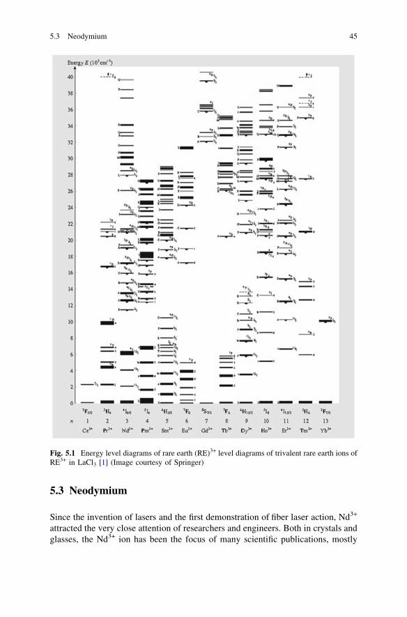
5.3 Neodymium

Since the invention of lasers and the first demonstration of fiber laser action, Nd3+

attracted the very close attention of researchers and engineers. Both in crystals andglasses, the Nd3+ ion has been the focus of many scientific publications, mostly

Fig. 5.1 Energy level diagrams of rare earth (RE)3+ level diagrams of trivalent rare earth ions ofRE3+ in LaCl3 [1] (Image courtesy of Springer)

5.3 Neodymium 45

because of Nd:YAG lasers, which became the main solid-state laser used for manyindustrial and scientific applications. Being a major active medium during the eraof nuclear fusion, the scientific study of Nd3+ in glasses is enormous. Taking intoaccount the similarity in energy-level positions of Nd3+ in different glass matrices,this section presents the spectroscopic information for Nd3+ in one of the mostdeveloped, most studied, and most widely used glass active media: phosphateglass. An energy-level diagram of the most important laser transitions for this ionis shown in Fig. 5.2.

In Fig. 5.3, the absorption spectra of the Nd3+ ion in phosphate glass are shown.Strong absorption bands are shown at 583, 750, 802 and 873 nm, which corre-spond to the following transitions between Nd3+ energy levels:

4I9/2

4I11/2

4I13/2

4I15/2

4F3/2

E88

0nm

808n

m

1050

nm

1330

nm

900n

m

1500

nm

4F5/2

11360 cm-1

0 cm-1

1840 cm-1

4700 cm-1

12400 cm-1

3850 cm-1

Fig. 5.2 Energy-leveldiagram of the mostimportant laser transitions ofNd3+

Fig. 5.3 Absorptionspectrum of Nd3+ inphosphate glasses at roomtemperature [2] (Imagecourtesy of the OpticalSociety of America)

46 5 Spectroscopic Properties of Nd3+, Yb3+, Er3+, and Tm3+ Doped Fibers

4I9=2 ! 2G7=2;4G5=2; 4I9=2 ! 4S3=2;

4F7=2; 4I9=2 ! 2H9=2;4F5=2 and 4I9=2 ! 4F3=2,

respectively (see Fig. 5.3) [2]. Absorption transitions at *802 nm (as in crystals)are the most widely used for pumping of the Nd3+-doped fiber laser because of thematured and widely available AlGaAs laser diodes in the 805 and 810 nm spectralrange.

Figure 5.4 shows the stimulated emission spectrum of the Nd3+ ion in phos-phate glass. The strongest emission peaks are located at 900, 1,053, and 1,330 nm,which correspond to the following transitions between Nd3+ energy levels:4F3=2 ! 4I9=2; 4F3=2 ! 4I11=2 and 4F3=2 ! 4I13=2, respectively (see Fig. 5.1). At300 K, the measured and radiative lifetimes of the Nd3+ ion in phosphate glassdoped with less than 3 wt % are 300 and 330 ls, respectively. The stimulatedemission cross-section was calculated using the Fuchtbauer-Ladenburg formula(see Chap. 2), giving the following values for 900, 1,053, and 1,330 nm emissionlines at 300 K: 1.5 9 10-20, 5 9 10-20, and 0.75 9 10-20 cm2, respectively.Luminescence of Nd3+ ions starts quenching seriously in this glass at an Nd3+

doping level exceeding 5 wt % (5.36 9 1020 ions/cm3). The stimulated emissioncross section is almost independent of Nd3+ concentration and has the followingtemperature dependence [2]:

r32 Tð Þ ¼ r32 T0ð Þ � exp b� T0 � Tð Þ½ � ð5:3Þ

where T0 is the temperature at which the stimulated emission cross-section isknown. r32(T0), the stimulated cross-section (between laser upper level 3 andlower level 2), is measured or known, b = 4.3 9 10-4 K-1.

For completeness of representation and for comparison, it is useful to providehere absorption and emission spectra of Nd3+-doped silicate glass, which is widelyused in gain fibers. Figures 5.5 and 5.6 show the room temperature absorption andemission spectra of the Nd-doped silicate glass [3].

As shown in Figs. 5.5 and 5.6, Nd-doped silica glass (similarly to other Nd-doped glasses) demonstrates absorption bands at 590, 750, 805, and 890 nm. The

Fig. 5.4 Stimulatedemission cross-section of 3 %doped Nd-phosphate glass [2](Image courtesy of OpticalSociety of America)

5.3 Neodymium 47

absorption bands most used for diode pumped laser applications are 805 and890 nm. Fluorescence spectra demonstrate the strongest lines at 950, 1,065, and1,320 nm. Figure 5.6 shows the most widely used emission line near 1,065 nm,which corresponds to the 4F3=2 ! 4I11=2 optical transition of Nd3+. Table 5.1shows the Judd-Ofelt parameters of the Nd3+ ion in different glasses.

Fig. 5.5 Room temperature absorption spectrum of Nd-doped silicate glass [3]

Fig. 5.6 Room temperature fluorescence spectrum of the Nd-doped silicate glass on the 4F3=2 !4I11=2 transition [3]

48 5 Spectroscopic Properties of Nd3+, Yb3+, Er3+, and Tm3+ Doped Fibers

5.3.1 Nd3+ Fiber Laser Challenges

Similar to the situation in Nd3+-doped laser crystals, one of the most important andchallenging tasks in Nd-doped glasses (and therefore, in fiber lasers and amplifiers)is to achieve high-power laser or amplifier oscillation of the 4F3=2 ! 4I9=2 tran-sition (900–950 nm). Such importance is dictated by the possibility to achieve bluelaser operation if the fundamental frequency of such oscillator can be doubled as aresult of nonlinear frequency conversion. The main challenge comes from thethree-energy level nature of the 4F3=2 ! 4I9=2 transition (Fig. 5.7) and its com-petition with the four-energy level 4F3=2 ! 4I11=2 (1,050–1,150 nm) and 4F3=2 !4I13=2 (1,330 nm) transitions. Another challenge is related to the desired bestbranching ratio into the 4F3=2 ! 4I9=2 transition—usually the ones with low sol-ubility of Nd3+ (e.g., pure fused silica). Therefore, a low concentration of Nd3+ isan expense for desired spectroscopic parameters. However, this is partly com-pensated for by the naturally long length of the gain fibers in fiber lasers andamplifiers, which may require hundreds of meters in the case of cladding pumpedNd3+ lasers.

Table 5.1 Judd-Ofelt parameters for Nd3+ in different glass hosts

Glass matrix X2 � 10�20 cm2 X4 � 10�20 cm2 X6 � 10�20 cm2 Source

Silicate Li2O� 2SiO2ð Þ 3.4 4.5 4.6 [4]Phosphate

Na2O�MgO� 2P2O5ð Þ3.5 3.6 5.0 [5]

Borate Na2O�MgO� 2Ba2O5ð Þ 5.9 6.1 7.5 [5]Tellurite (composition is not

available from the source)4.2 3.1 3.5 [5]

2F5/2

E

920n

m

976n

m

1035

nm

976n

m

2F7/2

1090

nm

11630 cm-1

11000 cm-1

10260 cm-1

1490 cm-1

1060 cm-1

600 cm-1

0 cm-1

860n

m

ZPL

Fig. 5.7 Energy leveldiagram of the mostimportant laser transitions ofYb3+

5.3 Neodymium 49

5.4 Ytterbium

As a laser-active ion in solids, such as crystals and glasses, Yb3+ can offer severaladvantages compared with traditional Nd3+ ions. These advantages include alonger upper-state lifetime, a small quantum defect (which results in lower thermalload per unit of pump power), and absence of the excited state absorption andupconversion losses because of a simple energy-level diagram (see Fig. 5.4).Yb3+-doped laser-active glasses have strong and wide absorption bands near 915and 976 nm and are suitable for diode pumping by the robust InGaAs laser diodes.In addition, Yb3+-doped laser glasses have broad and sufficiently intense emissionbands in the spectral range between 950 and 1,200 nm, with a zero-phonon line at976 nm. Room-temperature excited state lifetime is *1 ms. Due to broad emis-sion lines, Yb3+-doped laser glasses (in particular, fiber lasers) demonstrate tunablelaser action in a wide spectral range, from 980 to [1,150 nm.

The energy-level diagram of the Yb3+ ion has two manifolds: the ground 2F7/2

state and the excited 2F5/2 state. An energy-level diagram of the most importantlaser transitions of this ion is shown in Fig. 5.7. Absorption and emission spectraof the Yb3+-doped silica glass are shown in Fig. 5.8.

There are two main absorption peaks of Yb3+ in glass at 915 and 976 nm, whichcorrespond to the transition from the lowest Stark sublevel of the ground 2F7/2 stateto the second and the first (the lowest) Stark sublevels of the 2F5/2 manifold,respectively (see Fig. 5.8) [6–8]. It can be seen that Yb3+-doped glass laser is aquasi-three-level laser at room temperature.

Table 5.2 summarizes experimentally measured oscillator strengths of Yb3+ inthree of the most commonly used glass matrices, increasing in the order of silicateto germanate to phosphate. Robinson and Fournier [9] determined the oscillatorstrengths of Yb3+ ions in several glasses from room-temperature absorptionspectra. They found that Yb3+ spectra (except for the line width) are almostidentical, including relative intensities of the bands. The authors therefore

Fig. 5.8 Absorption andluminescence spectra ofYb3+-doped glass [6–8](Image courtesy of Springer)

50 5 Spectroscopic Properties of Nd3+, Yb3+, Er3+, and Tm3+ Doped Fibers

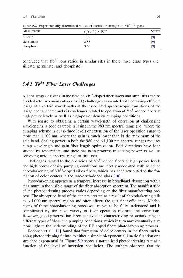
concluded that Yb3+ ions reside in similar sites in these three glass types (i.e.,silicate, germinate, and phosphate).

5.4.1 Yb3+ Fiber Laser Challenges

All challenges existing in the field of Yb3+-doped fiber lasers and amplifiers can bedivided into two main categories: (1) challenges associated with obtaining efficientlasing at a certain wavelengths at the associated spectroscopic transitions of thelasing optical center and (2) challenges related to operation of Yb3+-doped fibers athigh power levels as well as high-power density pumping conditions.

With regard to obtaining a certain wavelength of operation at challengingwavelengths, a good example is lasing in the 980 nm spectral range (i.e., where thepumping scheme is quasi-three level) or extension of the laser operation range tomore than 1,100 nm, where the gain is much lower than in the maximum of thegain band. Scaling power in both the 980 and[1,100 nm spectral ranges requirespump wavelength and gain fiber length optimization. Both directions have beenstudied by researchers, and there has been progress in scaling power as well asachieving unique spectral range of the laser.

Challenges related to the operation of Yb3+-doped fibers at high power levelsand high-power density pumping conditions are mostly associated with so-calledphotodarkening of Yb3+-doped silica fibers, which has been attributed to the for-mation of color centers in the rare-earth-doped glass [10].

Photodarkening appears as a temporal increase in broadband absorption with amaximum in the visible range of the fiber absorption spectrum. The manifestationof the photodarkening process varies depending on the fiber manufacturing pro-cess. The absorption band of the centers created as a result of photodarkening tailsto *1,000 nm spectral region and often affects the gain fiber efficiency. Mecha-nisms of these photodarkening processes are yet to be fully understood and iscomplicated by the huge variety of laser operation regimes and conditions.However, good progress has been achieved in characterizing photodarkening indifferent types of fibers and pumping conditions, which in turn may eventually givemore light to the understanding of the RE-doped fibers photodarkening process.

Koponen et al. [11] found that formation of color centers in the fibers under-going photodarkening fit into to either a simple biexponential kinetic function or astretched exponential fit. Figure 5.9 shows a normalized photodarkening rate as afunction of the level of inversion population. The authors observed that the

Table 5.2 Experimentally determined values of oscillator strength of Yb3+ in glass

Glass matrix f Yb3þ� �

� 10�6 Source

Silicate 1.82 [9]Germanate 2.83 [9]Phosphate 3.66 [9]

5.4 Ytterbium 51

photodarkening rate follows a seventh-order power dependency on the level ofinversion, as shown in Fig. 5.9. From studying two fibers with different levels ofYb3+ doping, the authors made preliminary conclusions on the photodarkeningprocess that takes place in the gain fiber. In particularly, it was suggested that thediscovered inversion dependence of the photodarkening process may be an indi-cation of a single mechanism (color-center formation) [11]. Seventh-orderdependence on population inversion may have significant influence on the fiberlaser operation. A pulse fiber amplifier may photodarken up to 105–107 timesfaster than even high-power CW fiber laser, where the level of inversion may besignificantly lower compared with a pulse regime [11]. Figures 5.9 and 5.10demonstrate the relative photodarkening rate versus level of inversion for differentoperational regimes of gain fiber operation.

Companies such as nLight (Liekki) and Nufern (East Granby, CT) achievedcertain success in developing highly photostable and highly Yb3+-doped fibers,which are commercially available.

Fig. 5.9 Measuredphotodarkening rate constantas a function of inversion.The slope of the log/log plotindicates a seventh-orderpower dependence [11](Image courtesy of SPIE)

Fig. 5.10 Normalizedphotodarkening rate as afunction of inversion,assuming a seventh-orderpower dependency. Deviceapplication regions withdifferent inversion levels arehighlighted [11] (Imagecourtesy of SPIE)

52 5 Spectroscopic Properties of Nd3+, Yb3+, Er3+, and Tm3+ Doped Fibers

5.5 Erbium

Er-doped fiber amplifiers and lasers are probably the most extensively studiedbecause of their importance in optical communication. Demand for 1.5 lm in-fiberlaser sources and amplifiers for optical signal transmission triggered an enormousnumber of research papers and successful commercial development. Several laserglasses have been developed as host materials for the Er3+ fiber lasers. Like othertrivalent rare earth ions, the spectroscopic properties of Er3+ in glass vary slightlyfrom one glass host to another. An energy-level diagram of the most importantlaser transitions of this ion is shown in Fig. 5.11.

Because RE3+ ions have similar spectroscopic properties within different glasshosts, consider the main spectroscopic properties of Er3+ in a metaphosphateglass host as an example [12]. Metaphosphate glass is a variation of phosphate glass.Er3+-doped metaphosphate glass was prepared with the following composition:mol. % of (59 - x/2)P2O5–17K2O–(15 - x/2)BaO–9Al2O3–xEr2O3, wherex = 0.01, 0.1, 1.0, 2.0, and 3.0 [12] (abbreviated glass notation is PKBAEr). We notehere that phosphate glasses are regarded as better hosts for Er3+ ions compared tosilicate glasses due to their higher phonon energy, more solubility of RE ions (whichallows the creation of highly concentrated fibers with short gain length), and smallerupconversion coefficient of the 4I13/2 level [13]. In particular, this is very importantfor Er3+-only doped gain fibers [14], in which high Er3+ concentration along with alow upconversion rate are desired.

Figure 5.12 shows the absorption spectrum of Er3+-doped metaphosphate glass,which is typical for all Er3+-doped glasses [12]. The spectrum demonstratesnumber of absorption lines spanning from 350 to 1,600 nm, which correspond tothe transition from ground energy level 4I15=2 to the upper levels of the Er3+

energy-level diagram. For fiber laser and fiber amplifiers applications, the mostimportant absorption bands are those located in the vicinity of 980 and 1,530 nm

4I11/2

E

1530

nm

1530

nm

1480

nm ZPL

980n

m

1600

nm

4I13/2

4I15/2

9700 cm-1

0 cm-1

6540 cm-1

6760 cm-1

10530 cm-1

Fig. 5.11 Energy leveldiagram of the mostimportant laser transitions ofEr3+

5.5 Erbium 53

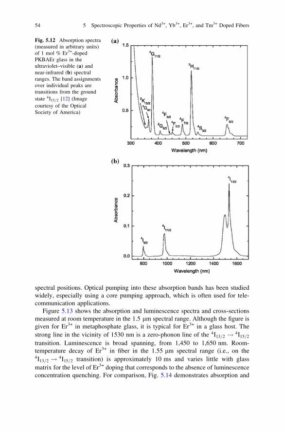
spectral positions. Optical pumping into these absorption bands has been studiedwidely, especially using a core pumping approach, which is often used for tele-communication applications.

Figure 5.13 shows the absorption and luminescence spectra and cross-sectionsmeasured at room temperature in the 1.5 lm spectral range. Although the figure isgiven for Er3+ in metaphosphate glass, it is typical for Er3+ in a glass host. Thestrong line in the vicinity of 1530 nm is a zero-phonon line of the 4I13=2 ! 4I15=2

transition. Luminescence is broad spanning, from 1,450 to 1,650 nm. Room-temperature decay of Er3+ in fiber in the 1.55 lm spectral range (i.e., on the4I13=2 ! 4I15=2 transition) is approximately 10 ms and varies little with glassmatrix for the level of Er3+ doping that corresponds to the absence of luminescenceconcentration quenching. For comparison, Fig. 5.14 demonstrates absorption and

Fig. 5.12 Absorption spectra(measured in arbitrary units)of 1 mol % Er3+-dopedPKBAEr glass in theultraviolet–visible (a) andnear-infrared (b) spectralranges. The band assignmentsover individual peaks aretransitions from the groundstate 4I15=2 [12] (Imagecourtesy of the OpticalSociety of America)

54 5 Spectroscopic Properties of Nd3+, Yb3+, Er3+, and Tm3+ Doped Fibers

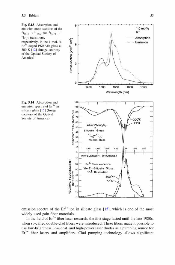
emission spectra of the Er3+ ion in silicate glass [15], which is one of the mostwidely used gain fiber materials.

In the field of Er3+ fiber laser research, the first stage lasted until the late 1980s,when so-called double-clad fibers were introduced. These fibers made it possible touse low-brightness, low-cost, and high-power laser diodes as a pumping source forEr3+ fiber lasers and amplifiers. Clad pumping technology allows significant

Fig. 5.13 Absorption andemission cross-sections of the4I15=2 ! 4I13=2 and 4I13=2 !4I15=2 transitions,respectively, in the 1 mol. %Er3+-doped PKBAEr glass at300 K [12] (Image courtesyof the Optical Society ofAmerica)

Fig. 5.14 Absorption andemission spectra of Er3+ insilicate glass [15] (Imagecourtesy of the OpticalSociety of America)

5.5 Erbium 55

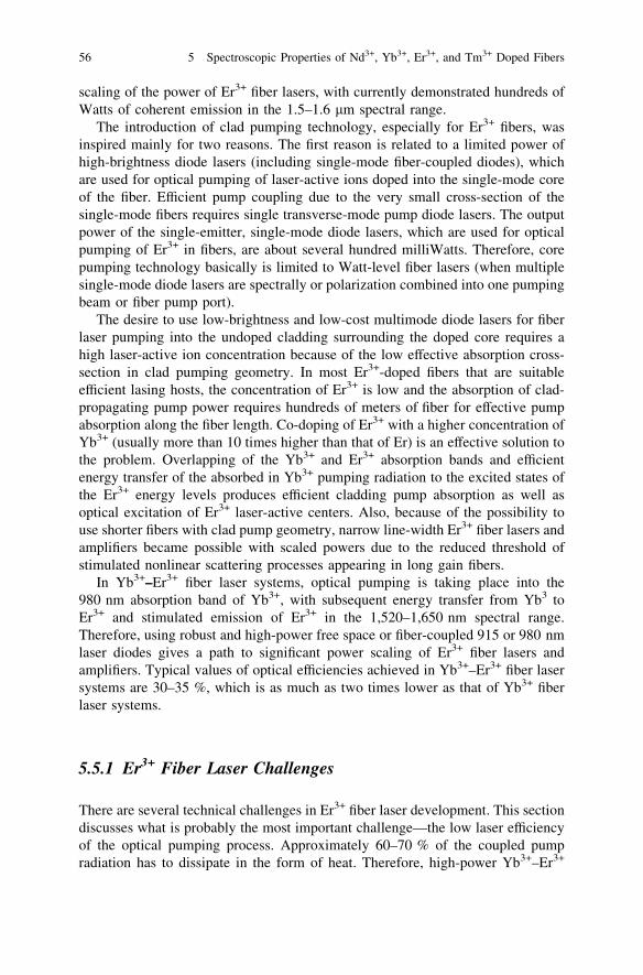
scaling of the power of Er3+ fiber lasers, with currently demonstrated hundreds ofWatts of coherent emission in the 1.5–1.6 lm spectral range.

The introduction of clad pumping technology, especially for Er3+ fibers, wasinspired mainly for two reasons. The first reason is related to a limited power ofhigh-brightness diode lasers (including single-mode fiber-coupled diodes), whichare used for optical pumping of laser-active ions doped into the single-mode coreof the fiber. Efficient pump coupling due to the very small cross-section of thesingle-mode fibers requires single transverse-mode pump diode lasers. The outputpower of the single-emitter, single-mode diode lasers, which are used for opticalpumping of Er3+ in fibers, are about several hundred milliWatts. Therefore, corepumping technology basically is limited to Watt-level fiber lasers (when multiplesingle-mode diode lasers are spectrally or polarization combined into one pumpingbeam or fiber pump port).

The desire to use low-brightness and low-cost multimode diode lasers for fiberlaser pumping into the undoped cladding surrounding the doped core requires ahigh laser-active ion concentration because of the low effective absorption cross-section in clad pumping geometry. In most Er3+-doped fibers that are suitableefficient lasing hosts, the concentration of Er3+ is low and the absorption of clad-propagating pump power requires hundreds of meters of fiber for effective pumpabsorption along the fiber length. Co-doping of Er3+ with a higher concentration ofYb3+ (usually more than 10 times higher than that of Er) is an effective solution tothe problem. Overlapping of the Yb3+ and Er3+ absorption bands and efficientenergy transfer of the absorbed in Yb3+ pumping radiation to the excited states ofthe Er3+ energy levels produces efficient cladding pump absorption as well asoptical excitation of Er3+ laser-active centers. Also, because of the possibility touse shorter fibers with clad pump geometry, narrow line-width Er3+ fiber lasers andamplifiers became possible with scaled powers due to the reduced threshold ofstimulated nonlinear scattering processes appearing in long gain fibers.

In Yb3+–Er3+ fiber laser systems, optical pumping is taking place into the980 nm absorption band of Yb3+, with subsequent energy transfer from Yb3 toEr3+ and stimulated emission of Er3+ in the 1,520–1,650 nm spectral range.Therefore, using robust and high-power free space or fiber-coupled 915 or 980 nmlaser diodes gives a path to significant power scaling of Er3+ fiber lasers andamplifiers. Typical values of optical efficiencies achieved in Yb3+–Er3+ fiber lasersystems are 30–35 %, which is as much as two times lower as that of Yb3+ fiberlaser systems.

5.5.1 Er3+ Fiber Laser Challenges

There are several technical challenges in Er3+ fiber laser development. This sectiondiscusses what is probably the most important challenge—the low laser efficiencyof the optical pumping process. Approximately 60–70 % of the coupled pumpradiation has to dissipate in the form of heat. Therefore, high-power Yb3+–Er3+

56 5 Spectroscopic Properties of Nd3+, Yb3+, Er3+, and Tm3+ Doped Fibers

fiber laser systems require special attention to heat management. Such a lowpump-to-lasing conversion efficiency has challenged researchers to use longwavelength pumping schemes, especially those that fall into the resonantabsorption band of the Er3+ energy level system near 1530 nm. This approachemploys usage of 1,460–1,500 nm laser diodes. However, quasi-three energy levellaser operation requires fulfillment of certain reabsorption bleaching conditions(i.e., a significant reduction of optical absorption); therefore, it is not trivial,especially when low-brightness diode lasers are used in clad pumping geometry.On the other hand, much higher laser efficiencies have been demonstrated, espe-cially in core-pumping geometry due to the absence of the upconversion losses andsmall quantum defect for resonantly pumped Er3+ fiber lasers in the1,460–1,530 nm spectral range.

Current laser diodes operating in the 1.5 lm spectral range are at least twotimes less efficient than 980 nm InGaAs laser diodes when calculating electrical-to-optical efficiency; therefore, overall electrical-to-optical fiber laser efficiencystill requires improvements. However, less relaxed requirements for the heatmanagement expected from resonantly pumped Er3+ fiber lasers is a definiteadvantage for power scaling to multihundred Watt to kilowatt laser power levels.

5.6 Thulium

Thulium-doped fiber lasers and amplifiers are among the most interesting fiberlaser-based systems. They provide laser operation in the 1.47 and 1.8 lm spectralranges and fall into the so-called eye-safe range of optical wavelengths.

As a side note, laser manufacturers have referred to lasers with operatingwavelengths longer than 1,400 nm (mid to far infrared) as eye-safe. This eye-safespectral range is of great importance due to numerous military and industrialapplications. Wavelengths in this region are absorbed in anterior portions of thehuman eye (mainly the cornea) and therefore never reach the retina, which islocated at the inward backside of the eye and acts as a photosensitive screen. Thisis in contrast to the eye-hazardous portion of the optical spectrum of400–1,400 nm (visible and near infrared), where the anterior portions of the eyehave high transmittance and refractive power. Irradiance levels are typically fiveorders of magnitude greater at the retina than at the cornea for visible and nearinfrared wavelengths. Although wavelengths longer than 1,400 nm do not interactwith the retina, they can interact with the skin or cornea and cause a thermal injury.However, the eye-safe operation depends on the laser power level as well as thewavelength. High-power lasers, especially those working with high pulse energy(i.e., Q-switched or high average power lasers) may still damage the eye. There-fore, working with the laser in an eye-safe wavelength range requires often similarprecautions as those outside eye-safe spectral range.

Like in other RE-doped fiber laser systems, the main problems during devel-opment of efficient Tm3+ fiber lasers and amplifiers are connected with selecting a

5.5 Erbium 57

proper glass host material and Tm3+ ion concentration. The most efficient lasertransitions in Tm3+ are those between the 3H4 excited state and the 3F4 lower level(or 3F4 and 3H6; see Fig. 5.15). An energy-level diagram of the most importantlaser transitions of this ion is shown in Fig. 5.15.

Closeness of the 3H5 energy level position to the 3H4 excited state level requiresselection of those glass host materials that demonstrate low phonon energy tominimize nonradiative multiphonon relaxation after the excitation process. Amongall glass hosts for Tm3+ fiber lasers, tellurite glass matrices are of great interestbecause they demonstrate low phonon energy (energy of the highest phonon is780 cm-1) and a high refractive index of 2.19. Without losing the general natureof the Tm3+ glass system review and following Ref. [16], the spectroscopicparameters of Tm3+ ion in tellurite glass that are important for its main laser activetransitions at 1,470 and 1,800 nm wavelengths are presented here.

3F2,3

E

1800

nm

1487

nm

3H6

22500 cm-1

14700 cm-1

12610 cm-1

5500 cm-1

0 cm-179

3nm

3F4

3H5

3H4

1G4

8300 cm-1

2320

nm

295.5 us

2.16 ms

Fig. 5.15 Energy-leveldiagram of the mostimportant laser transitions ofTm3+

Fig. 5.16 Room-temperature absorption spectrum (a) and energy-level diagram (b) of Tm3+ intellurite glass [16] (Image courtesy of the Optical Society of America)

58 5 Spectroscopic Properties of Nd3+, Yb3+, Er3+, and Tm3+ Doped Fibers

Figure 5.16 shows an absorption spectrum and fragment of the energy-leveldiagram for the Tm3+ ion in tellurite glass. The six absorption bands (480, 675,700, 800, 1,200, and 1,700 nm) correspond to the optical transitions from theground 3H6 level to the 1G4, 3F2, 3F3, 3H4, 3H5, and 3F4, upper levels, respectively.

Figure 5.17 shows a long wavelength fragment of the luminescence spectrumof Tm3+ in tellurite glass when excited with a 793 nm laser line at roomtemperature.

These spectra shows optical transitions from 3H4 to 3F4 (1,487 nm) and from3F4 to 3H6 (1,800 nm) levels, respectively. As indicated in Ref. [16], peak posi-tions and bandwidths of the 1,487 and 1,800 nm bands remain unchanged withTm3+ concentration. Relative intensity variation of these two emission bands withchanging Tm3+ concentration is attributed to cross-relaxation processes betweenthese two optical transitions. Stimulated emission cross-section has been calcu-lated and its maximum value at a 1,800 nm wavelength is 0.65 9 10-20 cm2.

The room-temperature lifetime of Tm3+ ions in tellurite glass (low doping; i.e.,concentration quenching free limit) measured in Ref. [16] for 3H4 and 3F4 energylevels are 295.5 ls and 2.16 ms, respectively.

For comparison, Fig. 5.18 shows Tm3+ absorption and emission spectra in otherwidely used glasses. Table 5.3 summarizes the Judd-Ofelt parameters as well aslifetimes of 3F4 energy levels for different Tm3+ glasses.

5.6.1 Tm3+ Fiber Laser Challenges

Several challenges may determine the research and development directions ofTm3+-doped fiber lasers and amplifiers. One challenge is connected with obtainingan efficient gain and laser action in the 1,487 nm spectral range, which isimportant in resonant pumping of Er3+ fiber lasers and amplifiers and also can be agood replacement of costly and more complicated Raman lasers. Another

Fig. 5.17 Luminescencespectra of Tm3+ in telluriteglass for different doppingconcentrations of Tm2O3 [16](Image courtesy of theOptical Society of America)

5.6 Thulium 59

challenge is attributed to the gain and laser action in Tm3+ fibers under a pumpwavelength of *1,150 nm due to low quantum defect and promising values oflaser efficiencies; this is an alternative to AlGaAs laser diodes operating in the790–805 nm range, which are traditional pumping sources for Tm3+-fiber lasers. Aso-called two-to-one process with cross-relaxation (Fig. 5.19) has been used forpower scaling of Tm3+-fiber laser using clad pumping technology and 790 nm

Fig. 5.18 Absorption (left) and fluorescence (right) spectra of a Tm3+:germanate, b Tm3+:silica,and c Tm3+:phosphate (Reprinted with permission from [17] )

Table 5.3 Results of Judd–Ofelt analysis for Tm3+ in four different glasses [17]

Material Tm concentration(1020 ions/cm3)

X2

(10-20 cm2)X4

(10-20 cm2)X6

(10-20 cm2)

3F4 srad

(ms)

Tm:germanate 6.24 4.4 1.2 0.9 5.3��� 4.0 1.6 0.8 ���2.50 ��� ��� ��� 4.97

Tm:silica 2.37 3.7 2.3 0.6 7.0��� 6.23 1.91 1.36 4.563.52 ��� ��� ��� 6.3

Tm:borophosphate 3.99 3.6 0.7 1 8.3��� 9.8 1.9 3.4 ���

Tm:fluorophosphate ��� 4.12 1.47 0.72 ���Tm:phosphate ��� 5.7 3.0 0.8 ���

2.35 ��� ��� ��� 5.0

Reprinted with permission from [17]

60 5 Spectroscopic Properties of Nd3+, Yb3+, Er3+, and Tm3+ Doped Fibers

high-power diode lasers; this process lead to more than 60 % of pump-to-laserefficiency, which is higher than pumping quantum efficiency for this pumpwavelength [18].

Tm-fiber manufacturing technology for two-to-one process optimization has beendeveloped by Nufern for high-power applications. However, photodarkening in theTm3+ gain fiber may occur at high levels of pump power when pumping with shortwavelength (790–805 nm) laser diodes. In addition, existing but less intense infraredemission near 2.3 lm in Tm3+ glass has been observed and laser action has beenobtained [19].

Fig. 5.19 Cross-relaxationand laser operation scheme inTm3+ fiber during pumpingcircle with a 790 nm diodelaser

Table 5.4 Spectroscopic parameters of the most widely used laser active centers in silica fibersand calculated gain saturation parameters for each ion

Laser ionandpumpingscheme Q

Signal(emission)wavelengthkL � 10�7

(cm)

PumpwavelengthkP � 10�7 (cm)

Excitedstatelifetime s(s)

Emissioncross-section re

(cm2)

GainsaturationparameterIs ¼ hc

kLsreQ

(kW/cm2)

Nd3+ four-energylevel(Q = 1)

1,060 810 300� 10�6 5� 10�20 8.3

Yb3+ quasi-four-energylevel(Q = 1)

1,040 976 900� 10�6 0:6� 10�20 30 [6–8]

Er3+ three-energylevel(Q = 2)

1,540 1,480 0.01 0:4� 10�20 1.075

Tm3+ four-energylevel(Q = 1)

1,900 795 250� 10�6 0:7� 10�20 39.85

Planck constant h ¼ 6:626� 10�34 J� s; speed of light in silica glass is cSi & c/1.5 = 2 9

1010 cm/s

5.6 Thulium 61

Table 5.4 summarizes important spectroscopic parameters for fiber laserdevelopment of the most widely used rare earth ions, as well as calculated gainsaturation parameters for laser transitions. Note that the gain saturation parameterplays a central role in the fiber amplifier and fiber laser design.

References

1. G.H. Dieke, Spectra and Energy Levels of Rare Earth Ions in Crystals, 1st edn. (Wiley, NewYork, 1968)

2. J. Dong, M. Bass, C. Walters, Temperature-dependent stimulated-emission cross section andconcentration quenching in Nd3+-doped phosphate glasses. J. Opt. Soc. Am. B 21, 454–457(2004)

3. S.E. Stokowski, R.A. Saroyan, M.J. Weber, Nd-Doped Laser Glass Spectroscopic andPhysical Properties (Technical Report) (Lawrence Livermore National Lab., Livermore, CA,USA, 2004) Nov 15, Report number: UCRL-TR-208148

4. R.R. Jacobs, M.M. Weber, IEEE J. Quantum Electron. QE-12, 102 (1976)5. N.B. Brachkovskaia, A.A. Grubin, S.G. Lunter, Sov. J. Quantum Electron. 3, 998 (1976)6. A. Tünnermann, J. Limpert, A. Bruns, Diode-pumped fiber lasers, Chap. 4.3, Landolt-

Börnstein—Group VIII Advanced Materials and Technologies, 12, 125–139, in Landolt-Börnstein: Numerical Data and Functional Relationships in Science and Technology, ed. byW. Schulz (New Series, Part 12 Subseries), Advanced Materials and Technologies, vol. XV(Springer, 2008), p. 282

7. H.M. Pask et al., Ytterbium-doped silica fiber lasers: versatile sources for the 1–1.2 lmregion. IEEE J. Sel. Top. Quantum Electron. 1(1), 2–13 (1995)

8. R. Paschotta, J. Nilsson, A.C. Tropper, D.C. Hanna, Ytterbium-doped fibre amplifiers. IEEEJ. Quantum Electron. 33(7), 1049–1056 (1997)

9. ChC Robinson, J.T. Fournier, Co-ordination of Yb3+ in phosphate, silicate and germinateglasses. J. Phys. Chem. Solids 31, 895–904 (1970)

10. L.B. Glebov, Linear and nonlinear photoionization of silicate glasses. Glass Sci. Technol.75(C2) (2002)

11. J. Koponen, M. Söderlund, H. Hoffman, D. Kliner, J. Koplow, Photodarkening measurementsin LMA fibers. Proc. SPIE 6453, 64531E.1–64531E.11 (2007)

12. P. Babu, H.J. Seo, K.H. Jang, R. Balakrishnaiah, C.K. Jayasankar, K.-S. Lim, V. Lavín,Optical spectroscopy, 1.5 lm emission, and upconversion properties of Er3+-dopedmetaphosphate laser glasses. J. Opt. Soc. Am. B 24, 2218–2228 (2007)

13. S. Jiang, T. Luo, B.C. Hwang, F. Smekatala, K. Seneschal, J. Lucas, N. Peyghabarian, Er3+-doped phosphate glasses for fiber amplifiers with high gain per unit length. J. Non-Cryst.Solids 263–264, 364–368 (2000)

14. M. Dubinskii, V. Ter-Mikirtychev, J. Zhang, I. Kudryashov, Yb-free, SLM EDFA:comparison of 980, 1470 and 1530 nm excitation for the core- and clad-pumping. Proc.SPIE 6952 (2008)

15. E. Snitzer, Glass lasers. Appl. Opt. 5, 1487–1499 (1966)16. R. Balda, J. Fernández, S. García-Revilla, J.M. Fernández Navarro, Spectroscopy and

concentration quenching of the infrared emissions in Tm3+-doped TeO2-TiO2-Nb2O5 glass.Opt. Express 15, 6750–6761 (2007)

17. G. Turri, V. Sudesh, M. Richardson, M. Bass, A. Toncelli, M. Tonelli, Temperature-dependent spectroscopic properties of Tm3+ in germanate, silica, and phosphate glasses: acomparative study. J. Appl. Phys. 103, 093104.1–093104.7 (2008)

62 5 Spectroscopic Properties of Nd3+, Yb3+, Er3+, and Tm3+ Doped Fibers

18. G. Frith, B. Samson, A. Carter, D. Machewirth, J. Farroni, K. Tankala, Power Scaling790 nm-Pumped Tm3+-Doped Devices from 1.91 to 2.13 lm Photonics West, San Jose,19–24 Jan 2008

19. R.G. Smart, J.N. Carter, A.C. Tropper, D.C. Hanna, CW oscillation of Tm3+-dopedfluorozirconate fiber lasers at around 1,470, 1,900 and 2,300 nm when pumped at 790 nm.Opt. Commun. 82(5, 6), 563–570 (1991)

References 63

Chapter 6Propagation of Light and Modesin Optical Fibers

Distance transfer of electromagnetic energy (i.e., energy transfer between remotepoints in space) in the spectral range of optical frequencies (light) can be done bypropagation of an electromagnetic field in a dielectric waveguide. The mainproperties of this light propagation in an optical waveguide are determined by totalinternal reflection (TIR). TIR takes place when light that propagates in a mediumwith a refractive index of n1 can be reflected from the boundary between thismedium and another medium with a refractive index of n2, which is less than n1.The condition of TIR takes place under a certain angle (critical angle) of incidenceof light. The angle of TIR is given by the following expression:

sin HTIRð Þ ¼ n2=n1ð6:1Þ

Therefore,

HTIR ¼ arc sin n2=n1

ffi �

ð6:2Þ

On the other hand, the allowed distribution of electromagnetic fields across thefiber is referred to as the modes of the fiber. Fiber mode derivation can bedetermined by solving the Maxwell equation for a cylindrical waveguide. Intypical silica-core, silica-clad fibers, the core refractive index is very close to thatof the cladding. This condition is called a ‘‘weakly guiding approximation’’:

D ¼ ncore � ncladð Þncore

� 1 ð6:3Þ

where Dn = ncore - nclad is the refractive index difference and D is the relative (orfractional) refractive index difference of the mode.

Under this condition, the modes propagating in the fiber are linearly polarized(LP) modes characterized by two subscripts, m and n. Therefore, the full notationbecomes LPmn (the longitudinal components of the fields are small when D � 1).The LP modes are combinations of the modes found from the exact theory of thewave guide. The first subscript, m, gives the number of azimuthal, or angular,nodes (i.e., periodicity in the angular field distribution) in the electric field

V. Ter-Mikirtychev, Fundamentals of Fiber Lasers and Fiber Amplifiers,Springer Series in Optical Sciences 181, DOI: 10.1007/978-3-319-02338-0_6,� Springer International Publishing Switzerland 2014

65

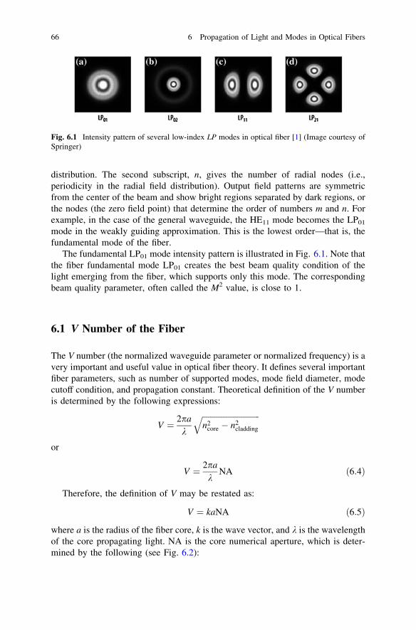
distribution. The second subscript, n, gives the number of radial nodes (i.e.,periodicity in the radial field distribution). Output field patterns are symmetricfrom the center of the beam and show bright regions separated by dark regions, orthe nodes (the zero field point) that determine the order of numbers m and n. Forexample, in the case of the general waveguide, the HE11 mode becomes the LP01

mode in the weakly guiding approximation. This is the lowest order—that is, thefundamental mode of the fiber.

The fundamental LP01 mode intensity pattern is illustrated in Fig. 6.1. Note thatthe fiber fundamental mode LP01 creates the best beam quality condition of thelight emerging from the fiber, which supports only this mode. The correspondingbeam quality parameter, often called the M2 value, is close to 1.

6.1 V Number of the Fiber

The V number (the normalized waveguide parameter or normalized frequency) is avery important and useful value in optical fiber theory. It defines several importantfiber parameters, such as number of supported modes, mode field diameter, modecutoff condition, and propagation constant. Theoretical definition of the V numberis determined by the following expressions:

V ¼ 2pa

k

ffiffiffiffiffiffiffiffiffiffiffiffiffiffiffiffiffiffiffiffiffiffiffiffiffiffiffiffiffi

n2core � n2

cladding

q

or

V ¼ 2pa

kNA ð6:4Þ

Therefore, the definition of V may be restated as:

V ¼ kaNA ð6:5Þ

where a is the radius of the fiber core, k is the wave vector, and k is the wavelengthof the core propagating light. NA is the core numerical aperture, which is deter-mined by the following (see Fig. 6.2):

Fig. 6.1 Intensity pattern of several low-index LP modes in optical fiber [1] (Image courtesy ofSpringer)

66 6 Propagation of Light and Modes in Optical Fibers

NA ¼ffiffiffiffiffiffiffiffiffiffiffiffiffiffiffiffiffiffiffiffiffiffiffiffiffiffiffi

n2core � n2

clad

� �

q

¼ n sin hð Þ ð6:6Þ

where n stands for the refractive index of the medium from which the light iscoupled into the fiber (or coupled out of the fiber) and h is the maximum angle ofincidence to couple light into the fiber (i.e., acceptance angle).

Another main fiber parameter is the normalized propagation constant b, whichis defined as follows [2]:

b ¼b2

k2

ffi �

� n2clad

n2core � n2

clad

ð6:7Þ

where k ¼ 2p=k and b=k ¼ D is the effective refractive index, b is the modepropagation constant, and 0 \ b \ 1. The value of k is the magnitude of the wavevector and defines number of waves per unit length. Therefore, the magnitude k isoften called the wave number. The number of the modes the step-index fiber cansupport may be determined using the following expression:

M � 4V2

p2ð6:8Þ

Figure 6.3 illustrates the so-called b–V diagram. If V \ 2.4048, a fiber supportsonly the fundamental LP01 mode. Thus, one can define a cutoff wavelength, kc,above which only a single mode is propagating in the waveguide with certaindimensions and refractive indices. The value b = 0 corresponds to the cutoffcondition, whereas b = 1 corresponds to the k = 0 condition.

Figure 6.3 shows the number of crossings of vertical line for a given value ofthe V number, with each curve corresponding to an individual LP mode, which inturn gives the number of modes propagating in the fiber. When the V number isless than 2.405, only the LP01 mode propagates. When the V number is greaterthan 2.405, the next LP mode can be supported by the fiber. For example, whenV = 3, both the LP01 and LP11 modes will propagate along the fiber (Fig. 6.3).

Fig. 6.2 Ray tracing inoptical fiber (schematic view)for definition of the fibernumerical aperture (h is theacceptance angle; hc is thecritical angle of the TIR)

6.1 V Number of the Fiber 67

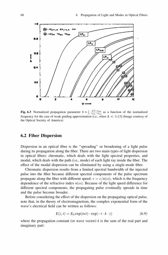
6.2 Fiber Dispersion

Dispersion in an optical fiber is the ‘‘spreading’’ or broadening of a light pulseduring its propagation along the fiber. There are two main types of light dispersionin optical fibers: chromatic, which deals with the light spectral properties, andmodal, which deals with the path (i.e., mode) of each light ray inside the fiber. Theeffect of the modal dispersion can be eliminated by using a single-mode fiber.

Chromatic dispersion results from a limited spectral bandwidth of the injectedpulse into the fiber because different spectral components of the pulse spectrumpropagate along the fiber with different speed: v ¼ c=n xð Þ, which is the frequencydependence of the refractive index n xð Þ. Because of the light speed difference fordifferent spectral components, the propagating pulse eventually spreads in timeand the pulse become broader.

Before considering the effect of the dispersion on the propagating optical pulse,note that, in the theory of electromagnetism, the complex exponential form of thewave’s electrical field can be written as follows:

Eðz; tÞ ¼ E0 expðiwtÞ � exp �i � k � zð Þ ð6:9Þ

where the propagation constant (or wave vector) k is the sum of the real part andimaginary part:

Fig. 6.3 Normalized propagation parameter b � 12 �

b=k�nclad

ncore�ncladas a function of the normalized

frequency for the case of weak guiding approximation (i.e., when D � 1) [3] (Image courtesy ofthe Optical Society of America)

68 6 Propagation of Light and Modes in Optical Fibers

k ¼ bph þ il ð6:10Þ

where l represents the attenuation constant and bph represents the phase constant.bph determines the change in phase per unit length along the propagation path andis equal to real part of the wave number. The phase constant is measured in units ofradians per meter. Therefore:

k ¼ 2pk¼ bph ð6:11Þ

To demonstrate the effect of dispersion on the propagating pulse, consider anoptical pulse with pulse width s. Also assume that the pulse propagates in a single-mode fiber. The minimum spectral width of the pulse Dxmin is inversely pro-portional to the pulse width (i.e., 1/s). Then assume that the spectral width of thepropagating pulse is much broader than the minimum spectral width:

Dx� Dxmin ð6:12Þ

It can be imagined that the overall spectrum of the pulse is a superposition ofseveral individual pulses with minimum spectral width of Dxmin. Each of theindividual pulses moves with group velocity:

Vg ¼dx

dbph

ð6:13Þ

where again bph is the phase constant and group velocity Vg is a speed at which thefiber mode power propagates along the fiber. In other words, group velocitydetermines the speed of energy propagation.

For completeness of the discussion, consider another important parametercalled phase velocity or Vph, which is determined by:

Vph ¼xk¼ c

n xð Þ ð6:14Þ

Phase velocity determines a speed at which phase (or wave front) of the wave ofcertain frequency (wavelength) propagates along the fiber.

The so-called group delay [4] demonstrates the effect of the dispersion on thepulse spreading in fiber:

Tg ¼1

Vgð6:15Þ

where Tg is the group delay time of a propagating pulse per unit length ofwaveguide. Due to chromatic dispersion, the group velocity depends on the fre-quency. Therefore:

d1

Vg

� �

¼d2bph

dx2

� �

dx ð6:16Þ

6.2 Fiber Dispersion 69

On a scale of finite frequencies, this expression becomes:

D1

Vg

� �

¼d2bph

dx2

� �

Dx ð6:17Þ

At the fiber entrance just after injection, a pulse with spectral width Dx can beconsidered as a pulse consisting of individual pulses with minimum duration s. Allpulses at the starting point coincide with each other and the overall pulse width hasthe same value of s. When the pulse starts propagating along the fiber, individualpulses travel at different speeds and require different times t to travel distance L inthe fiber. The individual pulse corresponding to given spectral component has atraveling time that can be calculated as follows:

t ¼ Tg � L ¼L

Vgð6:18Þ

Therefore, individual pulses with different frequencies will be spread along thefiber in the following time interval:

Dt ¼ L � D1

Vg

� �

ð6:19Þ

In turn, Eq. 6.19 gives the value of change of the original pulse Ds width over atraveling distance L:

Dt ¼ Ds ¼d2bph

dx2

� �

DxL ¼ � L

2� p� ck2 d2bph

dk2 þ 2kdbph

dk

Dx ð6:20Þ

Value d2bph=dk2� �

is the chromatic dispersion (more accurately,

Dchrom ¼ d2bph=dx2), determined by the fiber material [5], whereas dbph=dk isdetermined by the waveguide dispersion. Waveguide dispersion is only importantin single-mode fibers, where an evanescent wave of the fundamental modepropagates in the cladding. Because the refractive index in the cladding is lowerthan in the core, the cladding part of the mode travels faster than the part of themode that propagates in the core. In turn, this leads to the dispersion. Waveguidedispersion depends on the waveguide structure and is a part of chromaticdispersion:

Dchrom ¼ Dmat þ Dwg ð6:21Þ

Material and chromatic dispersion may have different signs depending on thepropagation wavelength (i.e., wavelength at which they are measured). In silicastep-index fiber, material and waveguide dispersions cancel each other out andtherefore lead to the minimization of chromatic dispersion near the 1,300-nmwavelength (Fig. 6.4). This fact attracts the attention of researchers in optical fibercommunications to the 1,300-nm spectral range. At this range, the pulse spreadcaused by chromatic dispersion results in limitations on the performance of the

70 6 Propagation of Light and Modes in Optical Fibers

optical transmission line. The chromatic dispersion curve can be approximated bya straight line near the wavelength of the zero dispersion. This line is called thechromatic dispersion slope (dashed line in Fig. 6.4). However, the propagation oflight with a wavelength close to 1,300 nm in silica fiber has measurable powerattenuation, especially at long distances; therefore, it is called ‘‘loss limited’’. Thisattenuation in silica fiber decreases at the 1,550 nm wavelength, where chromaticdispersion rises. Nevertheless, most optical communication systems operate in thevicinity of 1,550 nm because of a developed Er3+-doped fiber amplifier (its gainband covers the 1.55 lm range) and low attenuation. Therefore, operation in thisspectral range is chromatic dispersion limited.

Another dispersion type that needs to be mentioned is called the polarizationmode dispersion. This parameter is related to the fact that even an ideal single-mode fiber (i.e., the fiber that allows the propagation of only one fundamentaltransverse mode) actually supports two orthogonally polarized components of thesame fundamental mode. Note that an ideal single-mode fiber has the idealcylindrical symmetry and is stress free. However, such polarization degeneracybreaks in real life due to slight deviations from the fiber’s ideal cylindrical shape aswell as from stress introduced into the fiber in some cases, such as polarization-maintaining (PM) fibers. This deviation from the cylindrical symmetry and stress-induced anisotropy causes modal birefringence in the fiber, which in turn leads toslightly different propagation constants for two orthogonally polarized modes. Thiseffect also results in pulse broadening in optical fibers.

Fig. 6.4 General diagram of chromatic dispersion in a single-mode optical fiber

6.2 Fiber Dispersion 71

6.3 Polarization-Maintaining Fibers

In PM optical fiber, the plane of propagation light polarization is maintainedunchanged. This PM property of PM fiber is conditional, however. The conditionrequires the light polarization plane to be aligned at certain angle to the fiber stressgradient direction during coupling into the fiber. PM fibers are very important—not only in fiber laser applications, but also in optical telecommunications andinstrumentation. Usually, the PM property of the fiber is achieved by inducing acertain amount of stress in the core. This can be done through either elliptical coregeometry, a noncircular cladding profile, or so-called stress rods introduced intothe cladding surrounding the core. Accordingly, there are four main types of PMfiber geometries commonly used in current fiber laser technology: elliptical core,elliptical cladding, Panda profile, and Bow-tie profile (see Fig. 6.5). These PMfiber structures differ in the way that stress is introduced inside the waveguide tosuppress the cross-coupling of propagating power along two perpendicularlypolarized fiber modes.

Among all existing PM fiber types, the most widely used are Panda geometry-based fibers [6]. This geometry provides low loss, high optical quality, andsuperior uniformity along the whole length of the fiber. Commercial Panda fibershave been developed in different configurations, including large core([30–35 lm). Preservation of the circular core geometry gives the Panda-typestructure an additional advantage in the case of gain fibers. Technology of intro-ducing Panda stress rods into the cladding involves careful design, includingcladding space requirements. For gain fibers, technologists usually grow non-PMcore-doped fiber with a cladding diameter sufficient for introduced Panda stressrods. Later, after the laser/gain test is successful, stress rods are added during thenext run into the cladding surrounding the core, creating a PM fiber structure ofPanda type. The direction along the line where Panda rods and the core are locatedis called the slow axis; the perpendicular direction is called the fast axis.

PM fiber does not work as a polarizer (as it may seem to) but rather as a PMwaveguide transmitter of optical waves. Only light coupled into the fiber alongslow or fast axes will maintain its polarization plane. Launching the light into thefiber along planes other than those of slow or fast axes will not lead to the PM

Fig. 6.5 Different types of polarization-maintaining fibers (Image courtesy of Nufern)

72 6 Propagation of Light and Modes in Optical Fibers

property of the waveguide. This is why careful angle alignment during PM fibersplicing is critical. In current PM splicing machines, the angle between the stressrods of two fibers needs to be aligned by less than 1–2�. With the recent devel-opment of photonics crystal fibers, in which cladding consists of a periodicair/solid structure, Panda-like configurations have been successfully implemented.

6.4 Laser Beam Quality (M2 Parameter)

The beam quality is an important parameter of the laser, although it has beendefined in different ways. For most laser industrial applications, it is a measure ofthe focusing capability of the beam. Comparing two different laser beams with thesame focusing optics, the beams with better quality will allow tighter focusing.However, different kinds of aberrations or diffraction effects, existing either infocusing optics or in the laser oscillator active media, may affect the focus abilityof the system as they alter the laser beam wavefront.

All laser beam quality definitions can be divided into two major categories.Historically, the first method was based on the comparison of the product of laserbeam radius at the beam waist and the far-field beam divergence angle of the beam[called beam parameter products (BPP)] with that of the fundamental modeGaussian beam. The BPP is expressed in units of mm�mrad. Another method isbased on the second moment of the laser beam intensity profile. This methoddefines beam quality using the so-called M2 parameter.

By definition, a Gaussian beam with diffraction limited divergence (i.e., TEM00

mode in open laser resonators or LP01 mode in circular optical fiber) has thehighest beam quality. Correspondingly, high-order Gaussian modes demonstratepoor beam quality. Other beams, such as those originating from unstable reso-nators, may not be Gaussian in nature but may also demonstrate high beam-qualityparameters. This topic, however, is beyond the scope of this book.

Introduced by Siegman [7, 8], the M2 parameter has become a major beam-quality standard. It has been widely used since the early 1990s, both by laserresearchers as well as in laser applications in industry. Following Siegman [9](with these relationships holding in the main axes system of the beam), considerthe second moment of the beam intensity profile I(x, y) in the rectangular coor-dinates x and y, which can be expressed as follows:

r2x ¼ 4 �

RR

ðx� x0Þ2Iðx; yÞdxdyRR

Iðx; yÞdxdyð6:22Þ

where x0 is the center of gravity of the beam. For symmetrical beams, the gravitycenter usually is along the beam propagation line.

Following the expression for the variation of the Gaussian beam spot sizew(z) along the distance of propagation:

6.3 Polarization-Maintaining Fibers 73

w2ðzÞ ¼ w20 þ

kpw0

� �2

� z� z0ð Þ2 ð6:23Þ

where z0 is the Gaussian beam waist location and w0 is the beam waist. It can beshown that the analogous expression (i.e., the quadratic free-space propagationrule) can be written for the second moment of the intensity, which is then:

r2xðzÞ ¼ r2

x0 þ r2hX � z� z0ð Þ2 ð6:24Þ

and

r2hX ¼ 4 �

R R

hx � hx0ð Þ2�IFFðhx; hyÞdhxdhyR R

IFF hx; hy

� �

dhxdhyð6:25Þ

where rx0 and rh are the variance at the beam waist and the variance of the angularspread of the beam departing from the waist, respectively; z0 is the location of thebeam waist along the z axis (i.e., along the axis of propagation); IFFðhx; hyÞ is thefar field intensity distribution and hx; hy are angular coordinates of its center ofgravity. The quadratic propagation dependence is valid for any real laser beam(Gaussian or not, coherent or partially incoherent, single mode or multipletransverse mode). It is also important to note that the quadratic dependence ofbeam width given above is valid only for the second-moment beam widthdefinition.

As it is known, the Gaussian beam intensity profile can be expressed as:

IðxÞ ¼ exp �2x2=w2x

� �

ð6:26Þ

By defining wx 2rx the expression for intensity becomes:

IðxÞ ¼ exp �x2=2r2x

� �

ð6:27Þ

From the above intensity profile, Siegman defined the spot size or beam widthof an arbitrary, non-Gaussian beam (i.e., beam from real life) as the following:

Wx 2rx and Wy 2ry ð6:28Þ

where W stands for a general beam width for arbitrary real beams. Note that for theideal Gaussian TEM00 beam, the corresponding Gaussian beam parameter is w.

With above definition, the beam width W will propagate in free space followingthe same rule as the Gaussian spot size w(z) does if one multiplies the far-fieldspreading of the beam by the factor M2. Therefore, one can write for any arbitrarybeam the following width propagation rule, taking into account introduced defi-nition of the second moment width:

W2x;yðzÞ ¼ W2

0x;0y þ M2x;y �

kpW0x;0y

� �2

z� z0x;0y

� �2 ð6:29Þ

74 6 Propagation of Light and Modes in Optical Fibers

where Mx and My are parameters of the arbitrary beam under consideration and

hx;y ¼ M2x;y

kpW0x;0y

ð6:30Þ

is the divergence of the arbitrary beam. One can see that M2x;y shows how many

times the arbitrary beam divergence is bigger than that of the fundamental modeGaussian beam:

h0 ¼k

pw0ð6:31Þ

Consequently, the near-field far-field product for an arbitrary beam can bewritten as follows:

W0x;0y �Wx;yðzÞ � M2x;y �

zkp; z!1 ð6:32Þ

As can be seen from Eq. 6.32, parameters M2x;y may be interpreted as a value or

a measure of the propagating beam quality. It is natural to conclude from the aboveexpression that M2 1 characterizes a single, fundamental-mode Gaussian beam(i.e., TEM00 mode or, in the case of optical fiber, LP01 mode). It is also natural toconclude that the M2 parameter defined above shows how many times the realbeam divergence is larger than that of a diffraction-limited beam.

Despite that the M2 approach is not ideal and does have limitations, it worksquite well and is presently considered as a standard in the laser industry.

6.4.1 Practical Recommendations on Beam QualityMeasurements Using the M2 Approach

Beam quality, defined by the M2 parameter, ranges from 1 (the case of a dif-fraction-limited TEM00 laser beam) and[1 (for the arbitrary beam with high-orderor distorted modes). The National Institute for Standards and Technology and theInternational Standards Organization established standards [10] for laser beamquality measurements based on the M2 parameter, which can be implemented by aset of beam diameter measurements. An interesting and detailed discussion ofdifferent aspects of the laser beam quality can be found in Ref. [11].

The previously mentioned formalism can be reduced to practical formulas tocalculate the M2 parameter through measurements. If the M2 parameter isexpressed as a ratio of the diameter-divergence product of the laser beam underconsideration (arbitrary beam) to the ideal diffraction-limited (TEM00) beamdiameter-divergence product. It can also be given by the square of the ratio of themultimode beam diameter to the diffraction-limited beam diameter:

6.4 Laser Beam Quality (M2 Parameter) 75

M2 ¼ W0meashmeas

w0h0

� �

¼ W0meas

w0

� �2

ð6:33Þ

where W0meas is the measured beam waist diameter, hmeas is the measured full-angle divergence, w0 is the calculated (i.e., theoretical) diffraction-limitedGaussian beam waist, and h0 is the diffraction-limited Gaussian beam divergence.Recall also the Rayleigh range of the Gaussian beam, which is defined as thedistance a beam propagates from its waist to grow its diameter by a factor of

ffiffiffi

2p

,denoted as zR. For the diffraction-limited Gaussian beams, the Rayleigh range isrelated to the beam waist as follows:

w0 ¼ffiffiffiffiffiffiffi

zRkp

r

ð6:34Þ

Therefore, by measuring the arbitrary beam’s Rayleigh range, one can calculatethe beam waist for so-called imbedded fundamental mode Gaussian beams. Usingan expression for the M2 parameter, where this value is defined as a square of theratio of the multimode (i.e., unknown) beam diameter to the diffraction-limitedbeam diameter, one can calculate the unknown beam M2 parameter. Figure 6.6demonstrates an experimental setup for M2 measurement using the Rayleigh rangeapproach.

The following procedure can be used for M2 parameter measurement:

1. Insert a focusing lens in the beam under consideration. Locate and measure thebeam focus by moving an available charge-coupled device (CCD) cameraalong the beam propagating axis and estimate the smallest spot size (initiallyalong one axis; i.e., x diameter).

2. Locate the positions of the spot size where it is twice the estimated waist (i.e.,minimum) size on either side of the focus.

3. The actual focus position lies exactly halfway between these two points. Locatethe position of the waist.

4. Move the CCD camera to the actual focus position and measure the focusdiameter, which becomes the W0meas value.

LensBeam source Beam waist Position W0meas

Position where beam diameter is 1.414W0meas

zR

Beam quality measurement set-upFig. 6.6 Experimental setupfor beam qualitymeasurement

76 6 Propagation of Light and Modes in Optical Fibers

5. Measure the Rayleigh range, ZR, by finding the place along the beam propa-gation axis where the spot size grows to

ffiffiffi

2p

= 1.414 times the focused (i.e.,minimum) spot size. Do this by moving the CCD camera toward the lens untilsuch spot size is found. The distance between the beam waist location (mini-mum size) and the location of the beam where the beam size is

ffiffiffi

2p

larger is theRayleigh range ZR.

6. Using the beam waist and Rayleigh range relationship for the diffraction-lim-ited Gaussian beam, calculate the imbedded Gaussian beam diameter, whichhas the same Rayleigh range as that of the beam under consideration:

w0 ¼ffiffiffiffiffiffiffi

zRkp

r

7. Calculate M2 parameter using the following above given formula, inserting thecalculated imbedded beam waist diameter and measured diameter of the beamunder consideration (focal spot size):

M2 ¼ W0meas

w0

� �2

ð6:35Þ

This value defines the M2 parameter along the x axis (i.e., M2x ).

8. Repeat this procedure for the y axis and determine the M2 parameter along theperpendicular direction (i.e., M2

y ).

For better measurement accuracy, one may consider measuring two Rayleighranges instead of one Rayleigh range (as is demonstrated here) and calculate theM2 parameter from there. The typical value of M2 for diffraction-limited or close todiffraction-limited laser beams is between 1 and 1.5. M2 values of more than 1.5typically point to a multimode beam.

References

1. A. Tünnermann, J. Limpert, A. Bruns, Diode-pumped fiber lasers, Chap. 4.3 in LaserSystems, Part 2, Landolt-Börnstein—Group VIII Advanced Materials and Technologies, vol.12 (Springer, New York, 2008), pp 125–139

2. L.B. Jeunhomme, Single mode fiber optics: principles and applications (CRC Press, 1990),p. 339

3. D. Gloge, Weakly guiding fibers. Appl. Opt. 10(10), 2252–2258 (1971)4. R.B. Dyott, J.R. Stern, Group delay in fiber waveguides. Electron. Lett. l7, 82–84 (1971)5. M. DiDomenico Jr, Material dispersion in optical fiber waveguides. Appl. Opt. 11(3),

652–654 (1972)6. K. Okamoto, T. Edahiro, N. Shibota, Polarization properties of single-polarization fibers.

Opt. Lett. 7(11), 569–571 (1982)7. A.E. Siegman, New developments in laser resonators. Proc. SPIE 1224, 2 (1990)

6.4 Laser Beam Quality (M2 Parameter) 77

8. A.E. Siegman, Defining, measuring, and optimizing laser beam quality. Proc. SPIE 1868, 2(1993)

9. A.E. Siegman, How to (Maybe) measure laser beam quality, in DPSS Lasers: Applicationsand Issues (OSA TOPS vol. 17) ed. by M.W. Dowley, OSA, Washington D.C. (1998),pp. 184–199

10. Lasers and laser-related equipment—Test methods for laser beam widths, divergence anglesand beam propagation ratios. ISO Standard 11146 (2005)

11. T.S. Ross, W.P. Latham, Appropriate measures and consistent standard for high energy laserbeam quality. J. Directed Energy 2(1), 22–58 (2006)

78 6 Propagation of Light and Modes in Optical Fibers

Chapter 7Fiber Laser Physics Fundamentals

After reviewing the basics of solid-state physics and spectroscopy as related tofiber laser gain media, this chapter shifts the focus to the general aspects of laserphysics—especially the branches that are very important for understanding theprinciples of fiber laser operation.

7.1 Population Inversion: Three- and Four-EnergyLevel Systems

Population inversion plays a central role in the field of laser physics because itprovides a means for electromagnetic wave amplification and oscillation. Tounderstand the phenomenon of population inversion, it is important to brieflyreview the basic statistics of the particles’ distribution at thermal equilibrium.

As was described in Chap. 2, the number of particles at two neighboring non-degenerated energy levels in thermal equilibrium follows the Boltzmanndistribution:

N2 ¼ N1 exp �E2 � E1

kBT

ffi �

¼ N1 exp � h � m0

kBT

ffi �

ð7:1Þ

where E2 [ E1 (and E2 - E1 = hv0) and v0 is the resonant frequency of thetransition between these two energy levels. Particles are able to occupy either level1 with population N1 or level 2 with population N2. The total number of particlestherefore is:

N ¼ N1 þ N2 ð7:2Þ

As already shown in Chap. 2, in thermal equilibrium the lower energy level ismore populated than the higher energy level; therefore, the atomic system does notemit light and is naturally relaxed. Even at elevated temperatures, the number ofatoms occupying high-energy level 2 increases, but it never exceeds populationof the lower level. As can be seen from the Boltzmann distribution formula in

V. Ter-Mikirtychev, Fundamentals of Fiber Lasers and Fiber Amplifiers,Springer Series in Optical Sciences 181, DOI: 10.1007/978-3-319-02338-0_7,� Springer International Publishing Switzerland 2014

79

Eq. (7.1), levels 2 and 1 may become equally populated only at infinite temper-atures. However, to achieve an optical gain through stimulated emission, oneneeds to achieve a non-equilibrium situation when the number of particles at theupper level is higher than that at the lower energy level. This non-equilibriumcondition (or inverted population condition) has been suggested to achieveamplification of electromagnetic waves. During the early years of laser physics,atomic states with inverted populations were called states with absolute negativetemperatures because, from the classic viewpoint of Boltzmann distribution, such asituation corresponds to absolute negative temperatures (which, in thermodynamictheory, is known as an unachievable condition). This consideration shows that,thermodynamically, the laser is an example of a system where optical emissionoccurs with a very small value of entropy [1].

Several ways have been suggested to achieve such non-equilibrium conditions(i.e., population inversion). There are two basic pumping schemes of laser oper-ation within the concept of creation of population inversion, which in turn divideall active media into corresponding two classes (or types): the so-called four-leveland three-level laser systems. Historically speaking, the three-energy-level systemwas the first to demonstrate laser action (Ruby laser). However, for most practicalapplications, the four-energy-level scheme found much wider applications in laserdevelopment and commercialization. This chapter reviews each of these laserpumping schemes in detail because they are very important for all types of lasers,especially fiber lasers and amplifiers. In these applications, energy-level diagramsand the nature of line broadening of optical transitions can often be described byintermediate situations (i.e., so-called quasi-three-level or quasi-four-levelschemes, rather than purely three- or four-energy level schemes).

7.1.1 Four-Level Laser Operational Scheme

Figure 7.1 demonstrates the four-energy-level scheme of laser operation, which isideal for most laser applications requiring the highest efficiency along with thelowest laser threshold. As one can see from Fig. 7.1, during the pumping process,atoms are excited from the ground level 1 to the excited level 2. Then, after fastnonradiative relaxation to energy level 3 (usually within sub-nanosecond to pico-second timescale), atoms decay spontaneously to level 4 and then again throughnonradiative relaxation from level 4, returning to the original ground level 1. This isthe full excitation circle of the four-energy-level scheme. Note that spontaneousdecay from level 3 to level 4 (which is a slow process, with durations spanning fromnano-seconds to milliseconds) is exactly the transition where laser action isexpected. After fast non-radiative relaxation from level 2, particles start accumu-lating at level 3, while level 4 remains unpopulated because of fast relaxation fromit to ground level 1. Therefore, to create inversion population between levels 3 and4, only one particle needs to appear at level 3. Thus, the basic requirement forcreation of the population inversion is that relaxation from level 4 to level 1 has tobe faster than spontaneous decay from level 3 to level 4.

80 7 Fiber Laser Physics Fundamentals

7.1.2 Three-Level Laser Operational Scheme

Figure 7.2 shows the three-energy-level scheme of laser excitation. The principaldifference between the three-energy-level scheme and the four-energy-levelscheme is that the lower laser level (i.e., level 4 in Fig. 7.1) and the lowest level(i.e., ground state; level 1 in Fig. 7.1) becomes a single level (Level 1 in Fig. 7.2).Therefore, after spontaneous decay, particles do not return to the unpopulatedterminal level, as was the case in the four-energy-level scheme, but they appear toreturn to the original, populated ground state instead. In other words, within thethree-energy level scheme, the laser-terminating level is always populated.Therefore, the requirements for creating inversion population between the twolaser levels are very strict.

More than half of the total particles have to be excited to the laser’s upper levelin the three-energy-level laser operation scheme in order to create populationinversion. This condition requires much higher excitation intensities as well asspecial care to eliminate re-absorption of the amplified light while it travels alongthe laser medium. All of these factors contribute to an increased laser threshold

PUMP

2

1

3

4

Fast, non-radiative relaxation

Fast, non-radiative relaxation

Spontaneous decay

Induced emission

Fig. 7.1 Four-energy-leveldiagram of laser operation

PUMP

2

1

3Fast, non-radiative relaxation

Spontaneous decay

Induced emission

Fig. 7.2 Three-energy-leveldiagram of laser operation

7.1 Population Inversion: Three- and Four-Energy Level Systems 81

and complicate the achievement of high laser efficiencies. Nevertheless, the three-energy-level laser operation scheme is very important and has many applicationsin fiber lasers and amplifiers.

In commonly used laser excitation conditions, when the laser medium is excitedby another laser or flash lamp, it is fundamentally impossible to create populationinversion in a two-energy-level scheme. However, while exciting an isolated two-energy-level scheme using a resonant pump light with a very strong electromag-netic field, one can create a condition in which the probability of the particle toappear in the upper or lower energy level becomes a time-dependent parameter.Oscillation of the population at each of the two levels begins at the so-called Rabifrequency [2, 3]. Broadening of the spectral lines and deviation of the real energy-level systems from two-level systems (due to Stark splitting) prevents easyobservation of this phenomenon in solid-state laser media.

7.2 Optical Fiber Amplifiers

7.2.1 Fiber Amplifier (General Consideration)

A fiber amplifier basically works on same physical principles as its bulk solid-stateanalogs. The purpose of the fiber amplifier is to amplify a less powerful opticalbeam, which is propagating either inside another fiber or in free space. In this way,the amplifier is ‘‘seeded’’ with a low-power laser beam; such an optical beam iscalled a seed. There are two fundamental types of fiber laser amplifiers: thosebased on doped cores and those based on doped cladding. Doped-cladding fiberamplifiers use the evanescent field amplification principle; although they exist,they are not commonly used. Therefore, this review concentrates on core-dopedfiber amplifiers.

In core-doped fiber amplifiers, the amplifying light propagates in the samevolume where laser-active centers are located. The next subclassification is usuallydone based on the way the pump is coupled and propagates inside the gain fiber.This pump propagation classification divides all amplifiers into core-pumped andcladding-pumped fiber amplifiers. Note that the same classification is valid forfiber laser oscillators. As it is known from main principles of laser physics, thelaser oscillator is a device that contains a laser amplifier put inside an opticalresonator. The laser resonator fundamental function provides positive feedback.

This chapter considers a laser amplifier (i.e., optical amplifier) based on thestimulated emission amplification principle only. Information on other fiber opticalamplifiers, such as those based on optical nonlinearities (e.g., optical parametricamplifiers and Raman or Brillouin amplifiers) is available elsewhere. In thisintroduction, the main physical processes that take place in optical amplifiers arebriefly reviewed. A theoretical consideration of the CW and pulse amplifiers arethen presented, followed by the derived main formulas that are important forpractical design.

82 7 Fiber Laser Physics Fundamentals

7.2.1.1 Gain Saturation

As will be shown by analytical expression later in this section, high-input opticalfluence does not increase indefinitely in an amplifier but rather saturates, leading toamplifier gain reduction. Obviously, even from the general consideration of energyconservation, the gain of the amplifier has to saturate because one cannot extractmore power from the amplifier than it was excited (pumped) with. Gain saturationplays an important role in theory and practice of optical amplification and oscil-lation. The gain saturation parameter (Is), which will be introduced later in thissection, is a very important and unique parameter of the gain medium; it is oftenused to analyze and compare different gain media for certain applications. Thisparameter also plays an important role in the calculation and design of lasersystems, including amplifiers.

The advantages of operating an optical fiber amplifier in the gain saturationregime are mainly the following:

1. Small power fluctuations in the input signal do not reflect to the same extent inthe output amplified signal

2. The fiber amplifier, which has multiple spectrally close input signals withvaried intensity, may work as a gain equalizer because smaller input signalpowers have higher gain (because of less saturation) and higher input powershave lower gain (because of a higher degree of saturation)

3. A saturated optical amplifier demonstrates a high energy extraction efficiency;therefore, the overall efficiency of the system is high.

7.2.1.2 Gain Narrowing

Gain narrowing is an effect that takes place in fiber amplifiers and lasers; it isresponsible for light bandwidth reduction during amplification process. The pro-cess is a result of the fact that, due to limited gain bandwidth (usually with a bell-like gain spectral profile) of the amplifier material, the central region of the signaloptical spectrum is a subject of higher gain than the spectral wings.

For the single-pass laser amplifier, the seed line width decreases with increasinggain. For the Lorentzian atomic line shape (see Chap. 2), the optical amplifier full-width, half-maximum (FWHM) gain spectral bandwidth can be written as [2, 3]:

Dx3dB¼FWHM ¼ Dxa �ffiffiffiffiffiffiffiffiffiffiffiffiffiffiffiffiffiffiffiffiffiffiffiffiffi

3GdB x0ð Þ � 3

s

ð7:3Þ

where x0 is the central frequency of the atomic transition, G xað Þ ¼ IðLÞIð0Þ ¼

exp 2 � g xð Þ�L� 2 � l � L� �

is the amplifier gain factor expressed in units of dB,Dx0 is the natural line width of the atomic transition, g(x) is the gain coefficient,and l is the loss coefficient.

7.2 Optical Fiber Amplifiers 83

Amplifier losses and laser intracavity losses have to be taken into considerationwhen analyzing the gain narrowing effect. In the field of fiber lasers, the gainnarrowing effect may play a positive role (when a smaller spectral line width isrequired) or a negative role (when designing so-called Amplified spontaneousemission (ASE) sources with a flattened spectral distribution of output poweracross the emission spectrum).

7.2.1.3 Amplified Spontaneous Emission

Being an incoherent process, ASE extracts stored energy from the fiber amplifierby depleting the inversion population by spontaneous emission amplification. Thephysical reason for the ASE is as follows. Once excited during the pumpingprocess, electrons in the upper energy level are decaying not only through stim-ulated emission but also through spontaneous emission, which in turn is a randomprocess that depends on the level of inversion created in gain fiber. Only a fractionof the photons emitted spontaneously in all directions falls within the Numericalaperture (NA) of the fiber and therefore will be guided inside the core where theseed propagates. While propagating along the core, the amplified portion of cap-tured ASE photons interact with other laser active centers and, as other photons,these spontaneous photons are amplified by the stimulated emission process.Because ASE is mostly confined in the core, it is one of the major phenomena thatsaturates the fiber amplifier power scaling in the case of telecom type fibers(NA = 0.12, Dcore = 5 lm).

The power spectral density of the spontaneous emission induced noise Ssp(v) isa function of the frequency and amplifier gain [2, 3]:

SspðmÞ ¼ G� 1ð Þ � nsp � hm ð7:4Þ

Total integrated ASE noise power is:

PASE ¼ SspðmÞ � Dm ð7:5Þ

The optical power of the ASE light at the output of the fiber amplifier istherefore determined by the following expression [2, 3]:

PASE ¼ nsp � G� 1ð Þ � hm� Dm ð7:6Þ

where Dv stands for FWHM of the output spectrum and G is the absolute amplifiergain (see details later in this chapter). nsp is the spontaneous emission factor, whichis determined by:

nsp ¼N2

N2 � N1� � ð7:7Þ

where Ni is the average population of level i over the whole fiber length. It isevident from the expression for nsp that output ASE power in the fiber amplifier is

84 7 Fiber Laser Physics Fundamentals

large when population inversion is low. When the population inversion is high,seed can only be amplified. When the population inversion is low, the seed photonscannot only be amplified but also can be absorbed on the same transition.Therefore, the seed photons that get absorbed in the low inversion amplifier canproduce not only stimulated emission but spontaneous emission as well.

Using large mode area fibers with core diameters of 30 lm in conjunction withlow NA of *0.06, one can significantly suppress the ASE process in high-powerfiber amplifiers.

7.2.1.4 Laser Amplifier Noise

The main source of noise in fiber optical amplifiers is ASE, which has a spectrumclose to that of the amplifier gain spectrum. The noise arising from forward-propagating ASE is only a direct concern to the amplifier system because it strikesthe detector along with useful signals. The backward-propagating ASE can stilldeplete the amplifier inversion and reduce the gain.

The existence of ASE in the amplifier (or laser) system is often a major factorrestricting output power scaling with increase of the pump. Although in solid-stateand other laser systems there are several approaches to suppress ASE, such aslaser-active medium geometry and surface profile optimization, fighting ASE ingain fiber is still a big challenge because of the long lengths and small core sizes.To achieve minimum noise, optical fiber amplifiers are usually operated in a gainsaturation regime with gain between 8 and 10 dB, leaving little room for ASE andincreasing depleted stored energy.

The noise figure in a optical amplifier is defined as:

Fn ¼SNRinput

SNRoutput

� 2ni ¼ 2N2

N2 � N1ð7:8Þ

where SNRinput=output stands for the signal-to-noise ratio at the input/output of theamplifier, ni is the population inversion factor (which is equal to 1 for an idealamplifier; i.e., four-level amplifier, where the population of the lower laser level iszero). Therefore, from Eq. (7.8), one can see that the noise figure of the idealamplifier is:

Fn � 2 or 3 dB ð7:9Þ

In practical fiber amplifiers, the noise figure usually falls into the range of6–8 dB.

7.2.1.5 Laser Amplifier Phase Shift

Qualitatively speaking, the phase shift in a single-pass laser amplifier has two maincontributors: (1) the so-called free-space phase shift, which is linearly proportional

7.2 Optical Fiber Amplifiers 85

to the optical frequency; and (2) the phase shift due to atomic transition. FollowingSiegman [2, 3], the total phase shift in a single-pass laser amplifier can beexpressed as follows:

exp �i� bðmÞ þ DbatðmÞð ÞL½ � � exp �i� utot mð Þ½ � ð7:10Þ

and

utot mð Þ ¼ b mð ÞLþ Dbat mð ÞL ¼ 2pmcþ bL

2v mð Þ0

0ð7:11Þ

where v(v) is the real part of the material susceptibility (sometimes called a dis-persive part of the atomic response) of the gain medium. The first term in theexpression for the total phase shift is the basic free-space phase shiftbðmÞL ¼ ð2pmLÞ=c ¼ 2pL=k, which appears while the wave propagates through thelaser medium. As mentioned, the free-space phase shift is linearly proportional tothe frequency. The second term in the expression for the total phase shift is thephase shift due to atomic transition, Dbat mð ÞL. The magnitude of the added phaseshift due to atomic transition is proportional to the net gain (or absorption) of theoptical wave propagating through the gain medium. It can be shown that for aLorentzian shape of the atomic transition, the added phase shift is related to theoptical gain by the following expression [2, 3]:

Dbat mð ÞL ¼ 2m� m0

Dm0� g mð ÞL ¼ 2

ðm� m0ÞDm0

L � g m0ð ÞDm=2ð Þ2

m� m0ð Þ2þ Dm=2ð Þ2ð7:12Þ

where g(v0) is the gain coefficient at the center of the emission line. Note that at theresonance frequency, when v = v0, the gain is maximum but the phase shift isequal to zero. The phase shift is negative for frequencies below the resonancefrequency and positive for frequencies above the resonance frequency. The free-space phase shift usually is a major contributing factor to the amplifier phase shift.

7.2.1.6 Other Processes in Optical Amplifiers

In addition to the previously mentioned phenomena, a few other processes have tobe considered during the design and development of practical fiber amplifiers,especially at elevated optical powers. The first and probably most challengingprocess is the parasitic reflections from end surfaces of the amplifier material (poorsplicing; i.e., poor optical contacts) or other surfaces of free space optics in anamplifier system, which can cause parasitic lasing or self-pulsing (i.e., amplifierpulsing without a seed). Started oscillation obviously depletes inversion andreduces achievable gain. Self-pulsing plays an important role in stability andcreating a damage-free condition of CW fiber lasers and amplifiers. The outputinstabilities of a CW pumped three-level fiber laser, with sustained self-pulsing orself-mode-locking [4, 5], have been investigated extensively. Instability mayfollow from the nonlinear dynamics of the laser signal and from population

86 7 Fiber Laser Physics Fundamentals

inversion. It was demonstrated that higher output coupler reflectivity and sup-pressed nonlinear scattering processes, such as SBS and SRS yield to substantiallysuppressed self-pulsing, which in turn creates a condition for damage-free CWoperation.

Other processes that take place during short pulse amplification and happenunder high pulse intensity are spectral broadening (due to some nonlinear effects)and amplifying pulse distortion.

7.2.1.7 Fiber Amplifier Gains and Losses

When dealing with three-energy-level systems or quasi-three-energy-level systems(as in the case of most widely used fiber lasers, such as Yb3+ and Er3+), one needsto take into account reabsorption losses of laser radiation at the oscillationwavelength. Following Pask et al. [6], this section provides a detailed descriptionof the gains and losses in fiber amplifiers. First, consider the critical pump powerPpcr required to achieve a gain coefficient of zero at a particular point in the fiber(i.e., to reach transparency for the signal/laser wavelength), which is given by [6]:

Ppcr ¼ Ahmp1s

ral

ðrelrap � repralÞð7:13Þ

where A is the core area cross section, h is the Planck’s constant, vp is the pumplaser frequency, s is the upper-level lifetime, r is the cross-section of the quantumtransition, and e, a, p, and l denote to the emission, absorption, pump, and laserwavelengths, respectively (i.e., rap stands for the absorption cross-section at thepumping wavelength).

It is assumed in this analysis that the only loss mechanism in the fiber dopedwith laser-active ions is related to the absorption transition of the laser-activecenter and any other sources of loss-like scattering are absent. However, modernoptical fibers demonstrate measurable scattering loss (although this loss is smalldue to advanced modified chemical vapor deposition [MCVD] technology).Typical loss in modern fibers, especially those used for telecommunicationapplications (i.e., undoped), is on the order of *0.2 dB/km; for doped fibers, theloss varies from 0.01–0.1 dB/m, depending on the wavelength of laser operationand the gain fiber under consideration. Because typical fiber amplifier gain is in theorder of 10–30 dB/m, today’s state-of-the art MCVD or DND technology providevery efficient gain fibers, offering more than 75 % power conversion efficiencies(in the case of Yb3+ amplifiers and lasers).

The pump saturation power of the absorption transition of the optical center canbe expressed as:

Ps ¼hmpA

rep þ rap

� �

s/p

ð7:14Þ

7.2 Optical Fiber Amplifiers 87

where /p is the pumping quantum efficiency (for the Yb3+ ion, it is *0.92 whenthe seed wavelength is 1,064 nm and pump wavelength is 976 nm—a typicalexample of this type of amplifier).

The small-signal (unsaturated) gain for the whole length of the fiber amplifier isgiven by:

G0 ¼ g0L ¼/p rel þ ralð ÞsPa

Ahmp� NralL ð7:15Þ

In an approximation of the constant inversion along the fiber length, theabsolute gain factor of the fiber amplifier of the length L is therefore:

G ¼ PðLÞPð0Þ ¼ exp G0½ � ð7:16Þ

where Pa is the absorbed pump power, N is the laser-active center concentration,and L is the gain medium length. Note that expression NralL indicates totalabsorption loss in the whole length of the gain fiber at laser oscillation wavelength.In the general case of the varied inversion along the gain fiber, the absolute gainfactor should be integrated along the whole fiber length:

G ¼ exp½Z L

0g0ðzÞdz�: ð7:17Þ

For a high pumping level when gain coefficient g0 cannot be considered, a smallvalue saturated gain coefficient, g, can be expressed as follows:

g ¼ g0

1þ I=Isð7:18Þ

where I is the amplified light intensity and Is is a so-called gain saturationparameter, defined as an intensity of the amplifying beam in active medium atwhich the small-signal (unsaturated) gain coefficient g0 is reduced by 50 % (i.e.,half). In turn, the gain saturation parameter with good approximation can bedefined as the following general formula:

Is ¼hmL

ðrel þ reaÞs¼ hmL

relsQð7:19Þ

where Q ¼ 1þ rea=rel, and with good degree of accuracy Q = 1 for four-energy-

level systems (i.e., when rel � rea) and Q = 2 for three-energy-level systems(i.e., when rel � rea).

The stored energy in the four-level solid-state laser amplifier can be defined bythe following expression [2, 3]:

Est ¼ hmLNV ¼ g0IsV ð7:20Þ

88 7 Fiber Laser Physics Fundamentals

where V is the amplifier gain volume and N is the concentration of laser-activecenters created during the pumping process.

Note that the expressions for gain saturation parameters have been originallyderived for homogenously broadened lines, such as those appearing in crystals(e.g., YAG, ruby). However, in glass host materials, such as Yb3+ or Nd3+-dopedglasses, cross-relaxation processes are very fast (i.e., those processes responsiblefor excitation energy transfer between individual homogeneously broadenedspectral components within inhomogeneously broadened envelopes). For fastcross-relaxation in-homogeneously broadened host materials, it was shown that theprevious formulas are valid with good degree of accuracy. It is also evident fromthese expressions that, in three-energy-level transitions, gain saturates faster thanthat of four-energy level scheme.

The single-pass gain in fiber amplifiers, expressed in units of dB, can be cal-culated using following formula:

g kð Þ ¼ 10 logI

I0

ffi �

¼ 10 log eR l

0gðzÞdz

¼ 10 log exp/p rel þ ralð ÞsPa

Ahmp� Nrall

� � ð7:21Þ

7.2.1.8 Pulse Amplification

Frantz and Nodvik [7] reviewed two important practical application cases of pulseamplification in laser amplifiers: (a) the square pulse shape and (b) the Lorentzianpulse shape. The details of the analytical expressions for each of these cases can befound in Ref. [7].

(a) Square pulse shape

Figure 7.3 illustrates how the ratio of the output photon density (fluence) to inputphoton density changes versus time in units of pulse width s when the square pulsehas been injected into the amplifier.

Figure 7.3 is typical for pulse fiber amplifiers with ‘‘chopped’’ seeds, boosted inthe high-power amplification stages of the system. One can see clear temporalnarrowing of the output pulse, which is evident from Frantz–Nodvik analyses. Dueto difficulties associated with Q-switched fiber laser master oscillators, the seedchopping approach is widely used. The Frantz-Nodvik theory provides a directpath for pulse profile analysis in such fiber amplifier systems.

(b) Lorentzian pulse

The fiber amplifier seeded with a Q-switched pulse from a master oscillator, asillustrated in Fig. 7.4, does not have a square shape. One can use the aboveexpression to calculate the gain. Unlike the square-pulse seeded optical amplifier,

7.2 Optical Fiber Amplifiers 89

in which the square shape changes and the front of the pulse narrows significantly,the Lorentzian pulse preserves its bell-shaped profile (Fig. 7.4). Absence of a steepfront can be useful for some considerations of the pulse propagation in fiberamplifiers with respect to damage mechanisms of the fiber amplifier material.

7.3 Fiber Laser Thresholds and Efficiency

The laser threshold is one of the most important parameters of the laser oscillator.It reflects not only the gain properties of the active medium but also all active andpassive losses in the laser cavity. Calculated laser threshold and laser slope effi-ciency give the researcher a full set of parameters to calculate laser output power atany level of pump power.

In this section, for simplicity, the basic formulas for fiber laser threshold andlaser efficiency are presented [8, 9]. In most cases, fiber laser is a longitudinallypumped system; therefore, the theoretical expressions for this type of excitationare used.

Fig. 7.3 Ratio of the outputphoton density to inputphoton density versus time inunits of pulse width for aninitially square-shaped pulse[7]. Curve (a) shows that thetotal number of photons perunit area in the travelingpulse is 4 9 1018 cm-2.Curve (b) shows that the totalnumber of photons per unitarea in the traveling pulse is4 9 1019 cm-2. (Reprintedwith permission from Frantzand Nodvik [7],COPYRIGHT AIPPUBLISHING LLC.)

90 7 Fiber Laser Physics Fundamentals

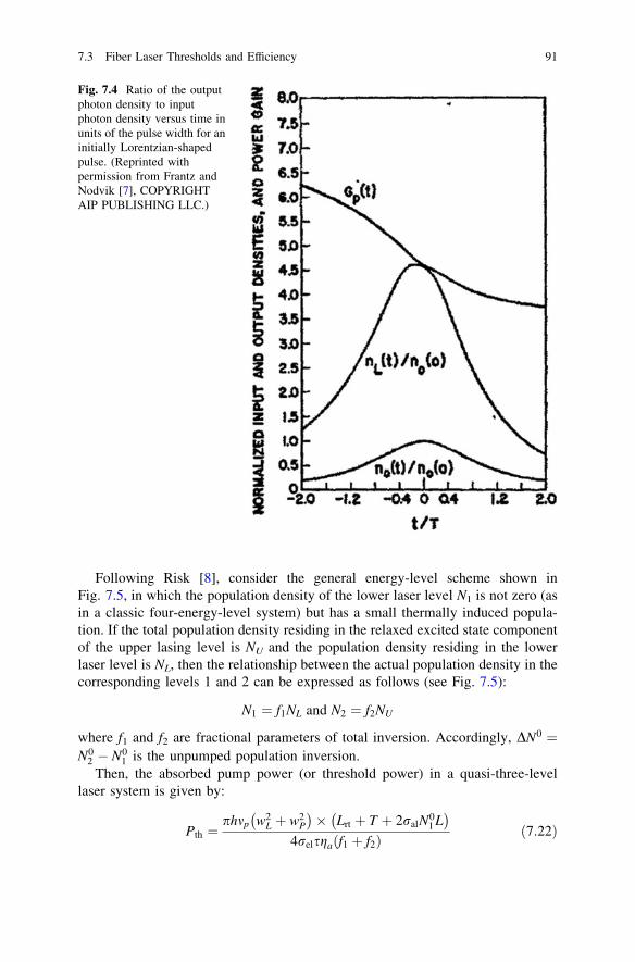
Following Risk [8], consider the general energy-level scheme shown inFig. 7.5, in which the population density of the lower laser level N1 is not zero (asin a classic four-energy-level system) but has a small thermally induced popula-tion. If the total population density residing in the relaxed excited state componentof the upper lasing level is NU and the population density residing in the lowerlaser level is NL, then the relationship between the actual population density in thecorresponding levels 1 and 2 can be expressed as follows (see Fig. 7.5):

N1 ¼ f1NL and N2 ¼ f2NU

where f1 and f2 are fractional parameters of total inversion. Accordingly, DN0 ¼N0

2 � N01 is the unpumped population inversion.

Then, the absorbed pump power (or threshold power) in a quasi-three-levellaser system is given by:

Pth ¼phmp w2

L þ w2P

� �

� Lrt þ T þ 2ralN01 L

� �

4relsga f1 þ f2ð Þ ð7:22Þ

Fig. 7.4 Ratio of the outputphoton density to inputphoton density versus time inunits of the pulse width for aninitially Lorentzian-shapedpulse. (Reprinted withpermission from Frantz andNodvik [7], COPYRIGHTAIP PUBLISHING LLC.)

7.3 Fiber Laser Thresholds and Efficiency 91

where wL and wP are the laser and pump beam waists, respectively; s is thefluorescence lifetime; T is the output mirror transmittance; and Lrt is the round-triploss, except for output coupling.

In the case of core-pumped fiber lasers, in which pump and laser beam waistsare similar, the following expression can be used to determine the laser slopeefficiency in the absence of excited state absorption:

gslope ¼dPout

dPp¼ T

ðLrt þ TÞkP

kLga

dS

dFð7:23Þ

where ga is the efficiency with which the pump photons are absorbed, dS=dF is theefficiency with which absorbed pump photons are converted to laser photons, andT= Lrt þ Tð Þ is the fraction of the laser photons that have been lost during round-tripdue to emission through output coupler from total loss. If we simplify the aboveformula for slope efficiency for the case when all absorbed pump photons areconverted to lasing photons and all pump photons have been absorbed, we can obtaina commonly used simplified expression for the laser slope efficiency, namely:

gslope ¼T

ðLrt þ TÞkP

kLð7:24Þ

Summarizing all analyses presented in this section, we can give an analyticalexpression for the laser output power in quasi-three-level case, which is the mostcommon case of fiber laser and fiber amplifiers energy-level configurations:

Pout ¼ gslope Pp � Pth

� �

ð7:25Þ

Note that in the case of Yb3+ fiber laser, where pumping can be accomplishedusing 976 nm excitation wavelength and laser can be observed at 1,030 nm

Fig. 7.5 General energy-level diagram [8]. (Imagecourtesy of the OpticalSociety of America)

92 7 Fiber Laser Physics Fundamentals

wavelength, the quantum defect ratio is kP=kL � 0:95, which in turn determinesthe maximum value of the laser slope efficiency. Typical Yb3+ fiber laser opticalefficiency is 70–80 %; slope efficiencies as high as 90 % have been achieved.

7.4 Gain and Loss in Laser Resonators

Knowing the amount of loss in the laser resonator is very important for under-standing the laser operation. There are several ways of measuring such losses. Oneof the most widely used techniques for four-energy-level lasers is based on themeasured laser threshold power as a function of varying output couplers. Thistechnique was first suggested by Findlay and Clay [10].

By measuring threshold pump power, Pth, and output coupler reflectivity, R,one can use the Findlay and Clay technique [10] to obtain the round-tripintracavity loss and small storage efficiency, gst (pump efficiency), which in turngives the value of small signal gain. By measuring the plot of ln(R) versus Pth, onecan readily derive these two important laser parameters using the followingfunction:

�ln Rð Þ ¼ 2 � gst

A� Is

ffi �

� Pth � Lloss ð7:26Þ

where the intercept of the y-axis yields –Lloss (loss), and the slope is proportional togst. Note that –Lloss = 2lL, where L is the length of the gain medium and l is thetotal internal loss coefficient due to absorption, scattering, and optical inhomoge-neity. The Findlay and Clay technique is valid for all systems and gives loss mea-surements independent of pump geometry, pulse shape, and pulse duration [10].

7.5 Fiber Laser Resonators

The physics of optical resonators used in fiber lasers is similar to the physics oftraditional laser resonators. The main differences are in intracavity componentsand geometry of the active medium. Intracavity optical components of fiber laserresonators have certain features, mostly related to the tolerance for optical dam-ages and fiber coupling. The active medium of fiber lasers is an optical waveguideusually with significantly longer length than in traditional lasers and very smalldiameter of the optical wave propagating medium. Long length and small fiberdiameters are the reasons for optical nonlinearities, which require special attentionin fiber laser development. The long length of the gain fiber in most fiber laserresonators is also the cause of challenges related to achieving short Q-switch pulsedurations. This section briefly reviews two fundamental types of laser resonators,which (as in other laser types) play an important role in practical fiber lasers.

7.3 Fiber Laser Thresholds and Efficiency 93

7.5.1 Linear Laser Resonators

A linear fiber laser resonator consists of two reflectors (usually mirror or fiberBragg gratings) set at the opposite ends of the optical cavity, gain medium in theform of laser-active ion-doped fiber, and other intracavity laser components tocontrol temporal and spectral properties of the fiber laser. In linear laser resonators,the resonator modes are usually considered as a superposition of two electro-magnetic waves traveling in opposite directions between cavity reflectors. Reso-nant frequencies of the linear resonator are given by the following expression:

m ¼ M � c0

2� n� L

�

ð7:27Þ

where M is the integer. Therefore, the frequency difference between two con-secutive (i.e., longitudinal) modes is given by:

Dm ¼ c0

2� n� Lð7:28Þ

where n is the refractive index of the medium where light propagates inside thelaser cavity.

Because light waves inside a linear laser resonator propagate in directionsopposite to each other, standing waves are created, which in turn have minimumand maximum interfering intensities. The minimum intensities of the standing-wave pattern of the intracavity laser field in the laser resonator are responsible forthe so-called spatial hole-burning effect; this affects the laser spatial gain distri-bution, which in turn favors the multispectral mode oscillation of the laser. On theother hand, because of the roundtrip nature of the light path inside the laserresonator and because the light propagates twice through the active medium duringthe cavity roundtrip, the laser gain (and loss) is accounted twice. This is a fun-damental feature of the linear laser resonator, differentiating it from the unidi-rectional ring laser resonator, which demonstrates no spatial hole burning effect.Ring laser resonators are described next.

Barnard et al. [11] developed an analytical model for rare-earth-doped fiberlasers. What makes this model appealing is that it provides formulas for the mainlaser parameters expressed in relatively easy measurable optical parameters of thesystem. According to Barnard et al. [11], in the case of a linear fiber laser cavity,the total fiber gain can be expressed as:

G ¼ expPplpPIS

p

PCSs PIS

p þ Pp

�� ls

0

@

1

A� L

2

4

3

5 ð7:29Þ

Here, the small signal gain coefficient is:

g ¼PplpPIS

p

PCSs PIS

p þ Pp

�� ls ð7:30Þ

94 7 Fiber Laser Physics Fundamentals

For the high pump level, the maximum gain is:

Gmax ¼ exp lp�

d� ls

� �

L� �

ð7:31Þ

The laser threshold is determined by the following expression (see Figs. 7.6and 7.7):

PLth ¼

hmpPCSs ½lsL� ln eRð Þ�

1� GmaxeRð Þ�dLinear laser cavity ð7:32Þ

where s = (s2 or s21) is the laser metastable level lifetime, vp is the pumpingphoton frequency, e = e1 e2 is the effective cavity transmission (with e1 and e2 asthe intracavity component single-pass transmissions), R ¼

ffiffiffiffiffiffiffiffiffiffi

R1R2p

is the effectivelaser cavity mirror reflectivity, d ¼ PCS

s =PISp is the ratio of the signal cross-satu-

ration power parameter and the pump intrinsic saturation power parameter, ls isthe small signal absorption coefficient at the signal wavelength and lp is the smallsignal pump absorption coefficient.

The signal cross saturation power PCSs is the parameter characterizing the

transfer of energy from the absorbed pump power to the signal. Parameters PCS;ISs;p

are defined as follows:

(a) (b)Fig. 7.6 Three-(a) and four-(b) energy-level laseroperation schemes

(a)

(b)

Fig. 7.7 Linear (a) and ring(b) fiber laser cavities

7.5 Fiber Laser Resonators 95

PCSs ¼

b2e

gpsAeff

ral þ b2erelð Þ three-energy-level schemeð Þ ð7:33Þ

or

PCSs ¼

b2e

gpsAeff

b2erel þ b12ralð Þ four-energy-level schemeð Þ ð7:34Þ

where s = (s2 or s21) is the upper laser level lifetime in the gain fiber, parameter

b2e for the three-energy-level scheme is N2=Ne ¼ b2e ¼ ð1þ s32=s2Þ�1 and for the

four-energy-level scheme N2=Ne ¼ b2e ¼1þ s32=s2 þ s1=s21 þ s1s32ð Þ= ss31ð Þð Þ�1 (both at the absence of seed power

Ps = 0); N1=N2 ¼ b12 ¼ s=s2 þ s32s1=s2s31 is the N1 and N2 energy-level popu-lation ratio at the absence of signal propagating power (i.e., Ps = 0); and

b12b2e ¼ b1e ¼ N1=Ne, also when Ps = 0.

PISp is the parameter that characterizes how pump absorption is saturated by the

pump light. PISp is the pump internal saturation parameter defined as:

PISp ¼

b2e

gpsAeff

rap þ b3erep

� � three-energy-level schemeð Þ ð7:35Þ

or

PISp ¼

b2e

gpsAeff

rpa þ b3erep

� � four-energy-level schemeð Þ ð7:36Þ

where b3e ¼ s32=s2ð Þ � b2e.Fiber laser slope efficiency in linear cavity can be expressed as follows:

glinear ¼gqe2 1� R2ð Þ

Teff;linear

� PISs

PCSs

1� GmaxeRð Þ�dh i

ð7:37Þ

where Teff;linear ¼ 1� R2e22

� �

þ 1� e21R1

� �

e22R2= eRð Þ is the effective output

transmission and R2 ¼ R1 � R2. One can calculate fiber laser output power inlinear cavity using the following formula:

Pout ¼ glinear Pp � Pth;linear

� �

ð7:38Þ

Optimum gain fiber length obtained in Ref. [11] for the case of linear cavity is:

Lopt ¼1

lp � d� lsln

Pp lp � d� ls

� �

PCSs ls eRð Þd

" #

ð7:39Þ

96 7 Fiber Laser Physics Fundamentals

7.5.2 Ring Laser Resonators

The ring resonator is another important type of laser cavity. It is defined as aresonator where the intracavity light travels along the ring type configuration. Thering cavity may be realized differently (i.e., using a folded type). To achieve acondition for phase shift of the traveling light wave during roundtrip of the cavityto be equal to 2p (the same condition as in the case of linear resonators), theexpression for resonant frequency can be given as follows:

m ¼ M � c0

n� Lring

ð7:40Þ

where Lring is the length of the closed loop path, M is an integer, and n is therefractive index of the fiber material. Ring laser resonators can support wavespropagating in opposite directions (i.e., clockwise and counterclockwise). How-ever, unlike linear laser resonators, ring laser resonators use a unidirectional device(e.g., an optical isolator), which allows the unidirectional propagation of the lightwave inside the laser cavity; the resonator becomes traveling wave because theconcept of the cavity mode and cavity resonance frequency are no longer definedas the same wave (as in the case of a standing wave resonator).

Following similar consideration of the cavity gain and loss, in traveling wave(unidirectional) ring resonators, the gain and loss have to be counted once. Lesscavity roundtrip gain obviously reduces laser gain; however, the absence of a hole-burning effect helps to achieve the single longitudinal mode of laser operation.Therefore, ring laser cavities are widely used for very narrow, single-longitudinalmode operation of the lasers.

However, the spatial hole-burning effect is essential for lasers in which theactive medium demonstrates a homogeneously broadening case of spectral linebroadening, where inversion of population is shared between different spectralcomponents of the laser modes. In the case of inhomogeneously broadenedspectral lines (e.g., glasses) spatial hole burning effect does not play a significantrole. In this case, a so-called spectral hole burning effect, which is a selectivebleaching of the spectral holes in the inhomogeneously broadened gain band of theoptical center [12, 13], plays a more important role in the multispectral modenature of the laser operation.

Following the results of Barnard et al. [11] and parameters introduced previ-ously, the ring fiber laser power threshold can be expressed as follows:

PRth ¼

hmpPCSs ½lsL� ln ejð Þ�

1� Gmaxejð Þ�d Ring laser cavity ð7:41Þ

where j is defined as the portion of the power that returns to the ring cavity by theoutput coupler. That is, if a filter coupler is used with 30:70 coupling ratio and30 % is recouped back into the cavity, then j = 0.3 and 1 - j = 0.7 is coupledout of the ring laser cavity. Ring fiber laser slope efficiency is defined as [11]:

7.5 Fiber Laser Resonators 97

gring ¼gqe2 1� jð Þ

Teff;ring

PISs

PCSs

1� Gmaxejð Þ�dh i

ð7:42Þ

where gq ¼ kp=ks is the quantum efficiency (i.e., ratio of pumping to signalwavelengths or corresponding photon energies); and Teff;ring ¼ 1� je is theeffective output transmission.

Using the formulas, one may obtain the ring laser output power using thefollowing general expression:

Pout ¼ gring Pp � Pth;ring

� �

ð7:43Þ

It is also important here to give an expression for optimum gain fiber lengthobtained in Ref. [11] for the case of ring cavity:

Lopt ¼1

lp � d� lsln

Pp lp � d� ls

� �

PCSs ls ekð Þd

" #

ð7:44Þ

References

1. N.G. Basov, Semiconductor lasers, Nobel lecture, Stockholm, Sweden, December 19642. A. Siegman, Lasers (University Science books, Mill Valley, 1986), pp. 12833. C.R. Giles, E. Desurvire, Propagation of signal and noise in concatenated erbium-doped fiber

optical amplifiers. IEEE J. Lightwave Technol. Lett. 9(2), 147–154 (1991)4. A. Hideur, T. Chartier, C. Ozkul, F. Sanchez, Dynamics and stabilization of a high power,

side-pumped Yb3+-doped double-clad fiber laser. Opt. Commun. 186, 311–317 (2000)5. A. Hideur, T. Chartier, M. Brunel, M. Salhi, C. Ozkul, F. Sanchez, Mode-lock, Q-switch and

CW operation of an Yb3+-doped double-clad fiber ring laser. Opt. Commun. 198, 141–146(2001)

6. H. Pask et al, Ytterbium-doped silica fiber lasers: versatile sources for the 1–1.2 lm region.IEEE J. Sel.Topics in Quantum Electron. 1(1), 2–13 (1995)

7. L.M. Frantz, J.S. Nodvik, Theory of pulse propagation in a laser amplifier. J. Appl. Phys.34(8), 2346–2349 (1963)

8. W. P. Risk, Modeling of longitudinally pumped solid-state lasers exhibiting re-absorptionlosses. J. Opt. Soc. Am. B 5, 1412– (1988)

9. M.J.F. Digonnet, C.J. Gaeta, Theoretical analysis of optical fiber laser amplifiers andoscillators. Appl.Optics. 24(3), 333–342 (1985)

10. D. Findlay, R.A. Clay, The measurement of internal losses in 4-level lasers. Phys. Lett. 20(3),277–278 (1966)

11. C. Barnard, P. Myslinski, J. Chrostowski, M. Kavehrad, Analytical model for rare-earthdoped fiber amplifiers and lasers. IEEE J. Quantum Electron 30(8), 1817–1830 (1994)

12. M. Bolshtyansky, Spectral hole burning in erbium-doped fiber amplifiers. J. LightwaveTechnol. 21(4), 1032–1038 (2003)

13. E. Desurvire, J.W. Sulhov, J.L. Zyskind, J.R. Simpson, Study of spectral dependence of gainsaturation and effect of inhomogeneous broadening in erbium-doped aluminosilicate fiberamplifiers. IEEE Photon. Technol. Lett. 2, 653–655 (1990)

98 7 Fiber Laser Physics Fundamentals

Chapter 8Main Operating Regimes of Fiber Lasers

8.1 Temporal Regimes

There are three main temporal regimes in laser operation:

1. Continuous-wave (CW) and free-running2. Q-switching3. Mode-locking.

As solid-state lasers, fiber lasers demonstrate the same types of operatingregimes. However, the physical processes that take place in gain media (the fibercore) create challenges that are unique to fiber lasers, mainly because of their smallcross-section dimensions compared with other active media (typical core diameterof diffraction-limited fiber lasers: 6–30 lm) and the very long length of gainmaterial (typically in the multimeter scale). In comparison, semiconductor lasersalso have gain material with very small cross-sectional dimensions, but the gainmaterial length is on the submillimeter scale. In addition, because of the rare-earthnature of fiber lasers’ active ions, energy storage in fiber laser systems is high. Inaddition to possibility of high energy/peak power pulse production by fiber lasers,these characteristics create challenges in nonlinear processes and damage pro-cesses, which have to be addressed during fiber laser design and development.

Like many other laser types, fiber lasers also can operate in the followingoperational modes:

1. Quasi-CW operation (QCW): When the pump source is opened only for shortperiod of time to prevent excessive heating of the gain medium or pump source.

2. Gain-switched operation: When the pump source (i.e., master laser; usuallyanother laser with high peak power and short laser pulse) is pumping anotherlaser (i.e., slave laser) only during short time periods within the time frame ofthe excited state lifetime of the slave laser source. Such excitation results indirect slave laser gain modulation. This technique is widely used for pumpingof high-gain solid-state lasers, such as Ti3+:sapphire, Cr4+:forsterite, Cr4+:YAG,as well as color center lasers.

V. Ter-Mikirtychev, Fundamentals of Fiber Lasers and Fiber Amplifiers,Springer Series in Optical Sciences 181, DOI: 10.1007/978-3-319-02338-0_8,� Springer International Publishing Switzerland 2014

99

3. Q-switched mode-locked operation: A combined regime when simultaneousmode locking and Q-switching of the laser takes place, such as when the Q-switched laser pulse envelope contains mode lock laser pulses, or under con-tinuous pumping conditions the laser generates a train of such complexlymodulated pulses.

This section provides a more detailed description of the three main laserregimes. It qualitatively describes the essential differences and challenges of CWand quasi-CW operational regimes and gives a detailed theoretical and qualitativeanalysis of the Q-switch and mode-lock operation. The motivation behind suchdifferent treatments of CW and high peak power regimes is in the different degreeof challenges and issues that researchers face during laser development. For CWfiber lasers, the main challenge is usually twofold: thermal management andnonlinearities. Because of the relatively low power level (on a watt to kilowattscale), nonlinearities that appear in CW lasers mostly affect power scaling at a verynarrow laser spectral line width in the kilohertz to megahertz range. In high peakpower lasers, such as Q-switched or mode-lock lasers, high peak powers of hun-dreds of kilowatts to megawatts not only restrict power scaling but also affectalmost all fiber laser parameters, such as spectral line width, damage threshold,and power stability.

8.1.1 CW and Free-Running Operation of Fiber Lasers

8.1.1.1 Qualitative Descriptions of the Essential Differencesand Challenges

Free-Running Operation

Free-running (or QCW) operation occurs when the laser-active medium is excitedby the pump pulses with energies enough to sustain laser operation; no otherintracavity laser components are used to control/modulate the laser pulse temporalprofile. Usually, the pump pulse duration is on the order of the active medium’slifetime. Such pumping results in a chaotic number of individual pulses. Pulsedoperation with significantly shorter pumping pulses and high enough peak powerto modulate the pumped laser gain is called gain switching (reviewed later in thissection).

The QCW regime of laser operation is usually applied when one needs to limitthermal effects in the laser-active medium. The pump is switched on only for acertain period of time, which is enough to reduce thermal effects, while the laserpumping process is close to its steady-state condition. For temperature-relatedissues, one may consider the so-called duty cycle (DC)—the parameter that showshow much time the laser is exposed to the pumping within one pumping circle:

100 8 Main Operating Regimes of Fiber Lasers

DC ¼ tpTp

ð8:1Þ

where tp is the laser pulse duration and Tp is the distance between pulses(i.e., period of the pulse train). For instance, if a diode laser with a pulse durationof 0.001 ms fires one periodical pulse at a frequency of 10 pulses per second(10 Hz), the diode laser DC is 0.00001 (0.001 %). The DC of CW operation istherefore equal to 100 % because there are no pulses.

Low-DC laser operation (a few percent or less) strongly reduces the thermaleffects in glass material, which in turn can reduce heat-related damage. At thesame time, applying techniques such as Q-switching still allows one to achievevery high peak power in a pulse-repetitive mode. When average power is not anissue and high peak power is required, the QCW operating regime is a very goodsolution because QCW laser diodes and laser diode arrays are able to deliver alarge amount of energy into the active medium within a short pumping pulse. Inthe case of fiber lasers, for which thermal management requirements are relaxedcompared with diode-pumped solid-state lasers, QCW operating regime is not verycommonly used unless high peak power is required, and it is not limited by bulkand surface damage of the fiber laser intracavity components. Note that thermalmanagement issues still exist in fiber lasers due to finite heat dissipation in gainfiber and thus need to be addressed. These issues usually occur in the case of highlaser average power and need to be taken into consideration during design anddevelopment. Therefore, the development of new fiber lasers with small quantumdefects is an important task for several applications.

CW Operation

In CW laser operation, the laser is continuously pumped and continuously oscil-lates in single or multiple longitudinal or transverse modes. The CW mode isapplied when one requires high average power and high power stability of the laseremission. The CW (or CW-pumped) fiber laser class is one of the most importantand demanded class of lasers for different industrial, military, and scientificapplications.

Like in all other types of lasers, especially solid-state lasers, the CW regime offiber lasers follows similar physics and theory. The main difference during thedesign and development of CW fiber lasers compared with solid-state lasers isassociated mostly with nonlinear scattering processes and other nonlinear pro-cesses (some of which should be taken into consideration when designing solid-state lasers as well). The other nonlinear processes mentioned previously areassociated with refractive index influence by high-power propagating inside thefiber core. These nonlinear processes include the optical Kerr effect, self-focusing,cross-phase modulation, and four-wave mixing. In addition, heat management anddamage of the bulk fiber glass and end surfaces are also essential during fiber laserdesign. Modeling of the main nonlinear scattering processes, such as stimulated

8.1 Temporal Regimes 101

Brillouin scattering and stimulated Raman scattering (discussed later), contributesto successful development.

Despite the widespread opinion that fiber lasers are generally a thermal problemfree system is just not valid opinion without considering level of power underdesign. Potential thermal management issues of CW fiber lasers as important asother with other design parameters. Most development of CW fiber lasers focuseson power scaling, which is connected to the selection of high-power fiber-coupledcomponents, such as isolators, pump couplers, and gain fibers with appropriatecore and clad diameters, as well as their numerical apertures.

Presently, the most developed CW fiber lasers systems are based on Yb3+, Er3+–Yb3+, Er3+, Tm3+, and Nd3+. Free space and fiber-coupled laser diodes used forpumping mentioned fiber gain materials are available from a number of companieswith power levels of several hundreds of watts. The main challenge in CW fiberlaser commercialization is connected with the development of commerciallyavailable high-power tolerant fiber-coupled laser components. The typical diodelaser wavelengths used for pumping applications are 793, 915, 980, 1,480, and1,530 nm. Note that several impressive CW fiber laser demonstrations have beenmade in achieving high-power performance. Yb3+-based fiber lasers operatingin the 1 lm spectral range demonstrate the following highest power levels(IPG Photonics, 2011): (a) 50 kW in the MM regime, with M2 & 30; (b) 10 kW inthe SM regime (i.e., close to diffraction-limited operation) with M2 & 2; and(c) 1.1 kW in the PM regime with M2 & 1.1. At the same time, the highest fiberlaser power for the 1.5 lm spectral range with diffraction-limited beam quality iscurrently in the range of several hundreds of watts, approaching the 1 kW levelobtained with the Yb3+–Er3+ system. Both Yb3+ and Er3+ fiber laser systems arepumped with InGaAs high-power diode lasers.

8.1.2 Q-Switched Operation of Fiber Lasers

Q-switched fiber lasers are currently one of the most important and challengingtypes of fiber lasers because they have probably highest potential (when operatingat high average power levels) for different applications (including nonlinear fre-quency conversion). However, they suffer from bulk and surface damage resultingfrom high peak power pulses that interact with fiber material for nanoseconds.

This section briefly reviews the basic theory of Q-switched laser operationalregimes and then mentions the challenges associated with this mode of laseroperation for high peak power fiber lasers. The section begins with generalQ-switch theory and then goes on to the CW-pumped, repetitive Q-switch regimein fiber lasers.

Q-switching of the laser resonator was first introduced in 1961 by Hellwarth [1]and experimentally demonstrated by McClung and Hellwarth in 1962. The mainidea of laser cavity Q-switching is that the laser should produce high peak powerand short pulses if the laser resonator Q factor changes rapidly from its highest

102 8 Main Operating Regimes of Fiber Lasers

value to the lowest (i.e., when intracavity loss changes from a high to low value).Initially, laser action is disabled by introducing a high loss (low Q condition).During such a low Q condition, pump power builds up the inversion population;when the latter reaches its peak value, the laser cavity Q factor switches to its highvalue (i.e., intracavity loss is removed). As soon as the laser cavity Q factor ishigh, radiation starts to build up inside the laser resonator from its spontaneousemission. After a certain period of time (buildup time or delay), due to the highvalue of the inversion population, the laser dynamically (through stimulatedemission) generates a high intensity pulse within a short period of time, which iscalled the Q-switched laser pulse or giant pulse (Fig. 8.1).

8.1.2.1 General Analyses of the Laser Q-Switched Operating Regime

Following the original work of Wagner and Lengyel [2], consider a laser cavitywith two end reflectors: gain medium and Q-switch device. Here, formulas forcalculating the main parameters of the laser emission in Q-switch mode of oper-ation are outlined.

In their analyses, Wagner and Lengyel [2] introduced the normalized variables:

�n ¼ N

N0ð8:2Þ

where N is the population inversion per unit volume and N0 is the number of activeions in the volume element (concentration).

Fig. 8.1 Inversion in theQ-switched pulse (Reprintedwith permission from [2])

8.1 Temporal Regimes 103

The normalized initial and final population inversions per unit volume for thehigh ð�niÞ and low ð�nf Þ Q state of the laser cavity during the pump process arerelated by the following transcendental equation:

�ni � �nf ¼ �nth � ln�ni

�nf

ffi �

ð8:3Þ

where the �nth population inversion density at the threshold can be expressed as:

�nth ¼ln 1

R1R2

h i

þ N0ralL

2N0 rel þ ralð ÞL ð8:4Þ

where R1 and R2 are reflectivity of the laser cavity mirrors, rel and ral are theemission and absorption cross-sections of the laser-active ion at laser wavelength,N0 is the total concentration of laser-active centers, and L is the fiber gain mediumlength. Output energy of the Q-switched laser pulse can be expressed as follows:

Ep ¼ hmL1c

VN0 � ð�ni � �nf Þ ð8:5Þ

where V is gain volume, N0 is the number of active ions in the volume element(concentration), h� mL is the photon energy at laser emission frequency, andc ¼ 1þ g2=g1, g1; g2 are degeneracies of the upper and lower laser levels. Notethat for a three-energy level system with no degeneracy g2=g1 ¼ 1, c = 2. For afour-energy level system, c = 1.

Consequently, the duration of the Q-switch pulse is:

tp ¼ Tres

�ni � �nf

�ni � �nth 1þ ln �ni�nth

� �h i ð8:6Þ

where Tres ¼ L � n=c � Ctot is the lifetime of the laser photon in the laser resonator;Ctot is the total, single-pass logarithmic loss of the cavity (useful laser logarithmicoutput plus intrinsic logarithmic loss; i.e., lnð1� Tint rÞ, where Tint r is the overallintrinsic loss of the intracavity medium), and n is the intracavity refractive index.Ctot can be expressed as follows:

Ctot ¼ � lnffiffiffiffiffiffiffiffiffiffi

R1R2p� �

þ ln 1� Tint rð Þ

ð8:7Þ

Therefore, the peak power of the Q-switched laser pulse is:

Ppeak ¼Ep

tpð8:8Þ

or

Ppeak ¼12

�nth log �nth=�nið Þ þ �ni � �nth½ � VN0hmL

Tres

ffi �

ð8:9Þ

104 8 Main Operating Regimes of Fiber Lasers

8.1.2.2 CW-Pumped, Repetitive Q-Switching Regime Analyses

We will start by estimating the maximum obtainable pulse energy from aCW-pumped Q-switched laser. The maximum extracted pulse energy from aCW-pumped Q-switched laser is given by [2, 3]:

Ep ¼ hmL1c

VDN ð8:10Þ

where hvL is the laser photon energy, V is the gain volume, and DN is the pop-ulation inversion difference per unit volume (non-normalized) between high (Ni)and low (Nf) Q mode of operation:

DN ¼ Ni � Nf ð8:11Þ

Note that because most practical CW-pumped lasers are four-energy level (orquasi-four-energy level), we will assume that c = 1. We also assume that NihhNT ,which is valid for four-energy-level laser systems, and N1 ¼ rap � Ip � s21 � Nth,which is an asymptotic value of the population inversion that is reached during thetime duration between laser pulses larger than the time of spontaneous decay s21

under a pumping intensity Ip. Then, solving a rate equation that describes the pumpcircle can give us the following expression for the time-dependent populationinversion:

NðtÞ ¼ N1 � N1 � Nf

� �

exp � t

s21

ffi �

ð8:12Þ

Consequently, for the repetitive Q-switching with pulse repetition rate f, themaximum time available for the inversion population to build up between laserpulses is:

Dt ¼ 1f

ð8:13Þ

Therefore, the expression for the value of population inversion achieved duringsuch a buildup of time becomes:

Ni ¼ N1 � N1 � Nf

� �

exp � 1s21f

ffi �

ð8:14Þ

In the approximation of ASE free operation (i.e., when Nf is negligibly small)and in the case when the laser is Q-switched with repetition rate f, we can expressthe population inversion difference per unit volume between high (Ni) and low (Nf)Q modes as follows:

DN ¼ Ni � Nf exp � 1s21f

ffi �

¼ N1 1� exp � 1s21f

ffi �� �ffi �

ð8:15Þ

8.1 Temporal Regimes 105

The output laser power in the CW regime is proportional to the difference ofpopulation inversions in the absence of stimulated emission ðN1Þ and that at thelaser threshold ðNthÞ and can be expressed as follows:

PCW ¼T

T þ LRT

ffi �

hmLVðN1 � NthÞ

s21ð8:16Þ

where s21 is the upper laser level lifetime, T is the transmission of the laser outputcoupler, and LRT is the laser cavity round-trip loss.

The threshold value of population inversion (similar to the previous paragraph)can be expressed as follows:

Nth ¼ln 1

R1R2

h i

þ N0rLaL

2 rLe þ rL

a

� �

Lð8:17Þ

Consequently, the Q-switched laser pulse energy can be expressed by:

Ep ¼ hmLVN1 1� exp1

s21f

� �ffi �

ð8:18Þ

or

Ep ¼ PCWs21 þ NthhmLVð Þ � 1� exp1

s21f

� �ffi �

ð8:19Þ

Knowing the fiber laser output power in the CW regime and the active ionspectroscopic parameters along with the gain fiber geometrical parameters, onecan calculate the Q-switched laser pulse energy.

Laser average power can be expressed as:

Pav ¼Tf

T þ LRT

ffi �

hmLV Ni � Nf

� �

ð8:20Þ

Finally, we will give an expression for the ratio of the CW-pumped Q-switchedlaser average power and output power in CW operation because this is animportant measure of the laser performance:

Pav

Pcw

¼ f s21

T

Ni � Nf

N1 � Nth

ffi �

ð8:21Þ

where T is the transmission of the laser output coupler.

8.1.2.3 Damage Problem

In optical materials, laser damage is a complex subject because of the many factorsaffecting the phenomenon, such as the presence of material volume defects andsurface polishing quality. Creating a single model that can describe laser-induced

106 8 Main Operating Regimes of Fiber Lasers

damage at different power levels and different qualities of the material irradiatedby the laser beam appears to be a very challenging task. Nevertheless, a few lawswere found to describe fairly well the bulk and surface damage thresholds ofdielectric materials, thus providing a ballpark value of the damage threshold.

The well-established square root law [3] describes the bulk damage of solid-state materials, such as crystal or glasses, and can be reasonably well applied tofiber laser systems. As is well known, the energy fluence J=cm2½ �, which corre-sponds to the limit when bulk damage start appearing in dielectric solids such ascrystals or glasses, can be expressed as follows [4]:

F � 25�ffiffiffiffi

tpp

ð8:22Þ

ðF � 10�ffiffiffiffi

tpp

for the case of surface damage Þ ð8:23Þ

where tp is the laser pulse duration expressed in nanoseconds. This formula worksquite well for nanosecond pulses longer than 5–10 ns, which is the case of most Q-switched fiber lasers. (For pulses close to 1 ns in duration, this formula may not beas accurate.) Assuming several meters of total fiber laser cavity roundtrip time,which gives a pulse duration of tens nanoseconds for the Q-switch pulses, we cansee that if the pulse duration is 25 ns, the maximum allowed laser pulse energyfluence when the laser fiber is in bulk damage-free condition is *125 J/cm2. If wetake the gain fiber diameter of 30 lm, which is almost the highest currentlycommercially available for diffraction-limited operations, the allowed pulseenergy is about 880 lJ, which in turn corresponds to about 30 kW of pulse peakpower. For comparison, Q-switched solid-state lasers such as Nd:YAG can easilyexceed tens of millijoules in pulse energies and over a megawatt of peak power indamage-free operation because of the bigger mode size of solid-state lasers. Thetypical damage pattern of the fiber laser output resulting from high peak poweroutput laser pulses is illustrated in Fig. 8.2.

Another challenge of high peak power fiber lasers (which include Q-switch andmode-locked systems) is to suppress the so-called self-phase modulation (SPM),described in more detail later in the book, and in such a way to preserve theoriginal or required spectral line width of the laser. This is usually achieved byproperly designed gain fiber core diameter and length, as well as the profile of thelaser pulse propagating inside the fiber. The ratio of the rise time of the laser pulseto the pulse duration is critical for SPM (and therefore the resultant laser spectralline-width), which can be minimized by using Gaussian laser pulses. The laser linebroadening due to SPM is maximized with super-Gaussian laser pulses.

Note that when the pulse duration approaches the 1 ns barrier (or less), theoptical breakdown processes, which include avalanche ionization and avalanchebreakdown, are too slow. Therefore, the damage threshold for short laser pulseswith sub nanosecond durations (or even below 10 ps) is usually higher. This factexplains why short-pulse fiber lasers (especially mode-locked fiber lasers,described in the next section) are more successful in scaling the fiber laser pulseenergy up to several millijoules and peak powers of *10 MW and higher.

8.1 Temporal Regimes 107

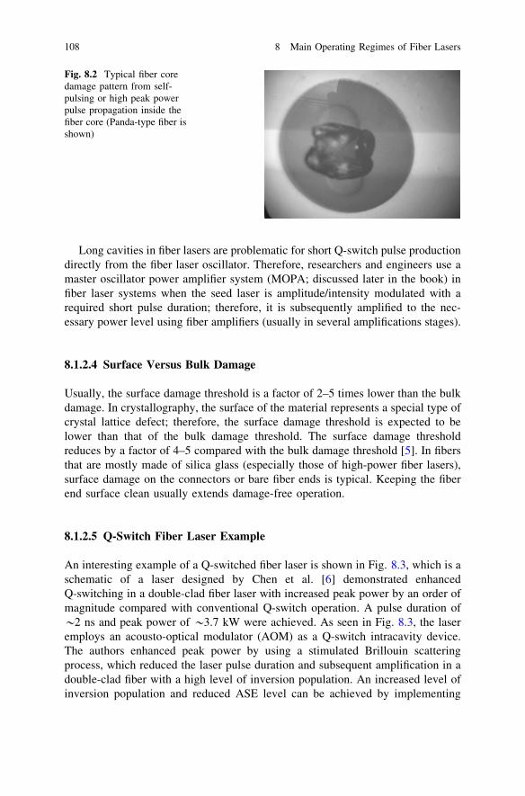
Long cavities in fiber lasers are problematic for short Q-switch pulse productiondirectly from the fiber laser oscillator. Therefore, researchers and engineers use amaster oscillator power amplifier system (MOPA; discussed later in the book) infiber laser systems when the seed laser is amplitude/intensity modulated with arequired short pulse duration; therefore, it is subsequently amplified to the nec-essary power level using fiber amplifiers (usually in several amplifications stages).

8.1.2.4 Surface Versus Bulk Damage

Usually, the surface damage threshold is a factor of 2–5 times lower than the bulkdamage. In crystallography, the surface of the material represents a special type ofcrystal lattice defect; therefore, the surface damage threshold is expected to belower than that of the bulk damage threshold. The surface damage thresholdreduces by a factor of 4–5 compared with the bulk damage threshold [5]. In fibersthat are mostly made of silica glass (especially those of high-power fiber lasers),surface damage on the connectors or bare fiber ends is typical. Keeping the fiberend surface clean usually extends damage-free operation.

8.1.2.5 Q-Switch Fiber Laser Example

An interesting example of a Q-switched fiber laser is shown in Fig. 8.3, which is aschematic of a laser designed by Chen et al. [6] demonstrated enhancedQ-switching in a double-clad fiber laser with increased peak power by an order ofmagnitude compared with conventional Q-switch operation. A pulse duration of*2 ns and peak power of *3.7 kW were achieved. As seen in Fig. 8.3, the laseremploys an acousto-optical modulator (AOM) as a Q-switch intracavity device.The authors enhanced peak power by using a stimulated Brillouin scatteringprocess, which reduced the laser pulse duration and subsequent amplification in adouble-clad fiber with a high level of inversion population. An increased level ofinversion population and reduced ASE level can be achieved by implementing

Fig. 8.2 Typical fiber coredamage pattern from self-pulsing or high peak powerpulse propagation inside thefiber core (Panda-type fiber isshown)

108 8 Main Operating Regimes of Fiber Lasers

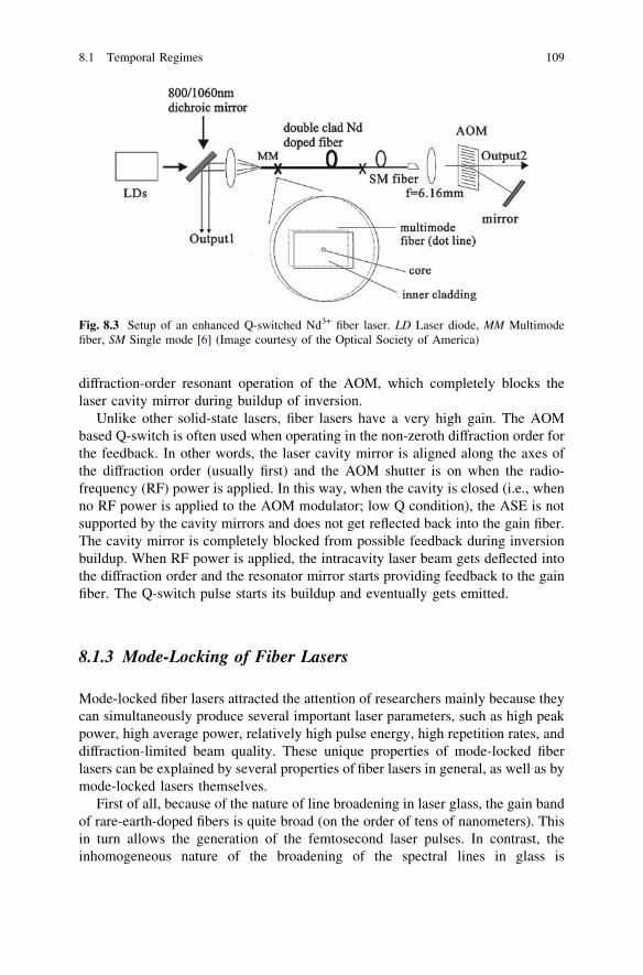
diffraction-order resonant operation of the AOM, which completely blocks thelaser cavity mirror during buildup of inversion.

Unlike other solid-state lasers, fiber lasers have a very high gain. The AOMbased Q-switch is often used when operating in the non-zeroth diffraction order forthe feedback. In other words, the laser cavity mirror is aligned along the axes ofthe diffraction order (usually first) and the AOM shutter is on when the radio-frequency (RF) power is applied. In this way, when the cavity is closed (i.e., whenno RF power is applied to the AOM modulator; low Q condition), the ASE is notsupported by the cavity mirrors and does not get reflected back into the gain fiber.The cavity mirror is completely blocked from possible feedback during inversionbuildup. When RF power is applied, the intracavity laser beam gets deflected intothe diffraction order and the resonator mirror starts providing feedback to the gainfiber. The Q-switch pulse starts its buildup and eventually gets emitted.

8.1.3 Mode-Locking of Fiber Lasers

Mode-locked fiber lasers attracted the attention of researchers mainly because theycan simultaneously produce several important laser parameters, such as high peakpower, high average power, relatively high pulse energy, high repetition rates, anddiffraction-limited beam quality. These unique properties of mode-locked fiberlasers can be explained by several properties of fiber lasers in general, as well as bymode-locked lasers themselves.

First of all, because of the nature of line broadening in laser glass, the gain bandof rare-earth-doped fibers is quite broad (on the order of tens of nanometers). Thisin turn allows the generation of the femtosecond laser pulses. In contrast, theinhomogeneous nature of the broadening of the spectral lines in glass is

Fig. 8.3 Setup of an enhanced Q-switched Nd3+ fiber laser. LD Laser diode, MM Multimodefiber, SM Single mode [6] (Image courtesy of the Optical Society of America)

8.1 Temporal Regimes 109

problematic for an energy-efficient narrow line-width in the glass laser oscillator.In the fiber laser, however, because of the high gain that comes from the long fiberlength and small core diameter, this type of glass laser is quite power efficient.Secondly, the high gain of fiber laser material allows the the fiber lasers to operatewith quite low pump powers and to use intracavity optical elements with relativelyhigh optical losses. Several dispersion compensation elements used in mode-locked fiber lasers cannot be used in traditional bulk solid-state lasers.

8.1.3.1 General Analysis of the Laser Mode-LockingOperating Regime

The regime of so-called mode-locking in lasers has been studied since the early1960s. In laser literature, several published reports on the mode-lock operation ofthe laser appeared in 1963. Since that time, laser mode-locking has been studiedextensively, both experimentally and theoretically [7]. This section gives a generalanalysis of the mode-locking regime of the laser operation.

In a free-running regime of operation, the laser oscillation is a complex com-bination of transverse and longitudinal modes without phase or amplitude corre-lation between modes. It is interesting to consider a situation in which the adjacentlongitudinal modes under passive (from passive intracavity devices) or active(from active intracavity device) modulation are forced into constant phase dif-ferences between each other. The process that leads to the establishment of such afixed adjacent longitudinal mode phase separation is called mode-locking.

During the mode-locking process, the laser system starts from noise, whichconsists of a series of short, irregular pulses with irregular phases. These pulses aretravelling back and forth between the two end mirrors of the laser resonator andare amplified by each transit in the laser-active medium. Kuizenga and Siegman[8] developed a theory describing mode-locked laser operation, predicting themode-locked laser pulse duration and the mode-locked laser spectral bandwidth.According to Kuizenga and Siegman [8], there are two competing mechanismsaffecting the creation of intracavity laser pulse width during the mode-lock regime.The first mechanism is due to the laser gain, which leads to the bandwidth-limitedgain factor and thus a reduction in the spectral width of the intracavity laser pulses,therefore lengthening the pulse width in each transit. The second mechanism isrelated to the effect of the modulator. The modulator shortens the pulse byaffecting the pulse tails due to the time-varying transmission of the modulator.

The equilibrium condition between the lengthening from the active mediumand shortening due to the modulator eventually determines what the steady-statepulse width is. The pulse gets shorter per transit, and one pulse per roundtrip timeis selected. In a spectral domain, the development of the mode-locked regime isrelated to the amplitude modulator’s modulating frequency. If the amplitude ismodulated with a sinusoidal modulation at a frequency Dxres, which is equal to theinverse value of the laser resonator round trip, the sinusoidal modulation of thecentral mode at the modulation frequency produces sidebands at x ± Dxres. These

110 8 Main Operating Regimes of Fiber Lasers

sideband frequencies injection-lock the adjacent modes, which in turn lock theirneighbors. According to Kuizenga and Siegman [8], in the case of the amplitudemodulation (AM) type of the intracavity optical modulator, the mode-locked laserpulse width and the laser pulse spectral bandwidth are as follows:

Dtp ¼ffiffiffiffiffiffiffiffiffiffiffiffiffiffiffiffiffi

ln 2 �ffiffiffi

2pp

p� g0 � L

dl

ffi �14

� 1fm � Dmg

ffi �12

ð8:24Þ

Dmp ¼ffiffiffiffiffiffiffiffiffiffiffiffiffiffiffiffiffiffiffiffi

2 � ln 2ffiffiffi

2pp

1� g0 � L

dl

ffi ��14

� 1fm � Dmg

ffi ��12

ð8:25Þ

where Dvg is the gain bandwidth of the laser medium; fm is the modulator fre-quency, which is expected to be close to the inverse value of the roundtrip time; g0

� L is the laser gain, and dl is the modulation depth. Note that for the case of AMmodulation, the pulse width–bandwidth product is Dtp � Dvg = 0.44. (Dvg is thespectral bandwidth of the mode-locked Gaussian pulse.)

Further assume that the laser demonstrates M longitudinal modes. The electricfield of an individual mode i can be expressed by the following formula [7]:

Emðz; tÞ ¼ E0msin xmt þ /m½ � � sin kmz½ � ð8:26Þ

where z is the coordinate along the propagation direction, E0m is the mode fieldamplitude, xm is the mode frequency, c is the speed of light, /m is the phase of thefield of the mth mode, and km ¼ xm=c is the wave-number of the mth mode.

If we introduce the central frequency x0 of the laser emission spectrum, thefollowing formula will describe the spectral position of each of the m longitudinalmodes:

xm ¼ x0 þ mDxres ð8:27Þ

where Dxres is a spectral separation of equidistant longitudinal modes of theFabry–Perot interferometer located on the frequency axis (expressed in hertz):

Dxres ¼2pc

Lres

¼ 2p� Dmres ð8:28Þ

In the case of fiber analysis, the speed of light c has to be replaced in thisformula by c/n, where n is the fiber material refractive index. Lres is the distancebetween laser cavity mirrors.

The resulting time dependent electrical field at point z can be expressed as:

Eðz; tÞ ¼X

M�1

m¼0

E0msin xmt þ /mð Þ � sin km � zð Þ ð8:29Þ

During a free-running regime, in the case of the homogeneously broadenedspectral line, individual laser modes undergo amplification during the round trip ofthe laser cavity across the whole gain band of the laser medium. However, because

8.1 Temporal Regimes 111

of the limited gain bandwidth and gain distribution inside the gain band, not allmodes amplify evenly. Those modes whose spectral frequencies are at the wingsof the gain profile undergo much less gain and therefore join the laser oscillationwith a delay, compared with a mode corresponding to the central frequency of thegain band. After a number of the round trips, the free-running laser spectralbandwidth therefore gets narrowed compared with the luminescence band andeven the spectral width of the gain band. The individual spectral modes, however,are not locked, and the mode phases are not related. In the case of multilongitu-dinal mode oscillation, the frequency resonances appear not only at the frequenciesof the longitudinal modes, but also on their nonlinear (parametric) frequencymixed modes because of the mode interaction. This in turn further complicatesachieving a steady state condition of the laser.

In addition, inhomogeneously broadened spectral lines, which take place infiber lasers, contribute additional characteristics to the laser dynamics. Thesecontributions are related to additional frequency variations, variations of therelaxation oscillations, and frequency interactions within the inhomogeneouslybroadened spectral line envelope [3, 9, 10]. Mode competitions and phase varia-tions inside the oscillating spectral band result in the variation of frequencies ofeach mode. The unlocked laser is therefore noisy. In general, if the laser cavitylifetime is long compared to the lifetime of the population inversion, the lasertends to be stable. If, however, the lifetime of the population inversion is longcompared to the laser cavity lifetime, the laser is unstable and demonstratesspiking in its temporary profile. On the other hand, when the mode phases arelocked, the field of each mode reaches the maximum at the same time. The modecompetition in a locked laser therefore does not exist, and all modes are equi-distantly positioned in the frequency domain. Note that the noise in mode-lockedlasers is significantly reduced by several orders of magnitudes compared with afree-running (i.e., unlocked) regime.

Consider the electric field inside the laser cavity. The intracavity electric field ina standing-wave laser resonator can be expressed as:

E z; tð Þ ¼X

M�12

m¼M�12

E0m exp ikmz½ � � exp �ikmz½ �ð Þexp ixmtð Þ ð8:30Þ

and

E z; tð Þ ¼X

M�1

m¼0

E0m exp ikmz½ � � exp �ikmz½ �ð Þexp i x0 þ mDxresð Þtð Þ ð8:31Þ

where z is the coordinate on the laser axis 0 \ z \ Lres, Lres is the resonator length,km is the wave vector of the mth individual mode:

km ¼xm

c¼ 1

cx0 þ mDxresð Þ ¼ k0 þ

m2pLres

ð8:32Þ

112 8 Main Operating Regimes of Fiber Lasers

where m = 0, 1, … M.The resultant field of the M modes is the following sum [7]:

E z; tð Þ ¼ exp i x0t � k0zþ p2

� �h i

X

M�12

m¼�M�12

E0mexp im Dxrest �pz

Lres

ffi �� �

þ exp i x0t þ k0z� p2

� �h i

X

M�1

m¼0

E0mexp im Dxrest þpz

Lres

ffi �� �

ð8:33Þ

Equation 8.33 shows that the field is modulated with the frequency Dxres insidethe pulse envelope. Therefore, the distance between individual pulses in theenvelope is equal to the laser cavity roundtrip trt. The front terms in each part ofthe above expression describe the light inside the laser cavity travelling to the rightand to the left. The terms under the expression maximize at z = 0 (one of thecavity mirrors) and t = 0, that is, in the points where the high-intensity pulse iscreated. The new maximum appears when t ¼ p=Dxres at a distance of z ¼ Lres,which corresponds to the location of the second laser cavity mirror.

When z = 0 (at one of the cavity mirrors), the intracavity electric field can beexpressed as:

E tð Þ ¼ 12

X

M�1

m¼0

E0mexp �i x0 þ mDxresð Þt þ i/mð Þ

þ 12

X

M�1

m¼0

E0mexp þi x0 þ mDxrestð Þ � i/mð Þð8:34Þ

All these modes will be locked once the following condition for phase isachieved:

u0 ¼ /1 ¼ � � � ¼ /m ð8:35Þ

If we assume for simplicity that, for all values of m, the amplitude of theindividual field is E0m ¼ E0 and the phase of individual field is /m ¼ 0, one canobtain the following sum for total electric field value:

E tð Þ ¼ 12

X

M�1

m¼0

E0exp i x0 þ mDxresð Þtð Þ þ 12

X

M�1

m¼0

E0exp �iðx0 þ mDxresÞtð Þ

¼ 12

E0 exp �ix0tð Þ exp �iMDxrestð Þ � 1exp �iDxrestð Þ � 1

þ exp þix0texp þiMDxrest � 1ð Þ

exp þiDxrestð Þ

ffi �� �

¼ E0sin2 MDxrest

2

� �

sin2 Dxrest2

� � cos x0 þ M � 1ð ÞDxres

2

ffi �

t

ð8:36Þ

8.1 Temporal Regimes 113

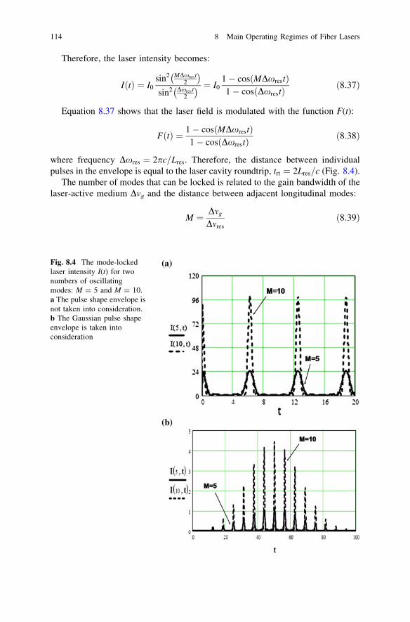
Therefore, the laser intensity becomes:

I tð Þ ¼ I0sin2 MDxrest

2

� �

sin2 Dxrest2

� � ¼ I01� cos MDxrestð Þ1� cos Dxrestð Þ ð8:37Þ

Equation 8.37 shows that the laser field is modulated with the function F(t):

F tð Þ ¼ 1� cos MDxrestð Þ1� cos Dxrestð Þ ð8:38Þ

where frequency Dxres ¼ 2pc=Lres. Therefore, the distance between individualpulses in the envelope is equal to the laser cavity roundtrip, trt ¼ 2Lres=c (Fig. 8.4).

The number of modes that can be locked is related to the gain bandwidth of thelaser-active medium Dvg and the distance between adjacent longitudinal modes:

M ¼ Dmg

Dmres

ð8:39Þ

Fig. 8.4 The mode-lockedlaser intensity I(t) for twonumbers of oscillatingmodes: M = 5 and M = 10.a The pulse shape envelope isnot taken into consideration.b The Gaussian pulse shapeenvelope is taken intoconsideration

114 8 Main Operating Regimes of Fiber Lasers

To estimate the mode-locked laser pulse-width, we assume that it correspondsto the half of the time span between zeros of the function F(t):

Dtp ¼2p

MDxres

¼ 2Lres

Mc¼ 2p

DxLð8:40Þ

where DxL ¼ MDxres is the total laser spectral band width.As a result of the uncertainty principle between the intensity of the individual

laser pulse and its phase, one can obtain the following expression for the shortestpulse obtainable during mode-locking operation of the laser, which is:

Dtp ¼C

Dmg� trt

Mð8:41Þ

where constant C is the time bandwidth product. Constant C is equal to 0.44 forGaussian-shaped pulses and 0.315 for sech2-shaped pulses. The latter is veryimportant in optical soliton laser oscillation and soliton pulse propagation. One cansee from Eq. 8.41 for the minimum pulse width of the mode-locked laser that theminimum pulse duration is inversely proportional to the number of the lockedlongitudinal modes. In other words, under similar other laser parameters, the morelongitudinal modes that are locked, the shorter pulse the laser is expected togenerate. Therefore, active media with very broad emission spectra (e.g., transitionmetals in crystals, color centers, liquid dyes, laser-active glasses) are the mostpromising laser materials for ultra short pulse generation. For the same interlongitudinal mode distance for the laser resonator mentioned above, laser gainmaterials may cover a very big number of spectral modes.

It is interesting to compare the laser intensities for two cases: free-running(unlocked) and mode-locked lasers. Assuming the laser demonstrates M operatingmodes, the peak and average power of the laser depend on the locking conditionsof the individual laser modes. In the case of unlocked lasers, both average andpeak power are proportional to the number of modes M:

PFR;AV � ME20m ð8:42Þ

Ppeak;FR;m � ME20m ð8:43Þ

In the case of mode-locked lasers:

PM�L;AV � ME20m ð8:44Þ

Ppeak;M�L;m � M2E20m ¼

trt

DtpPAV;M�L ð8:45Þ

Therefore:

Ppeak;M�L;m

PAV;M�L¼ M ð8:46Þ

8.1 Temporal Regimes 115

One can see that the ratio of the average powers for these two regimes equals to1, whereas the ratio of the peak powers is equal to M. One can also see that thepeak power of the most intense mode-locked laser pulse is M times higher than theaverage power of the same laser. Therefore, in mode-locked lasers, the peak powerhas a strong dependence on number of modes. By knowing the laser cavity’sgeometrical parameters, such as cavity length, the mode-locked laser averagepower, and pulse duration, one can estimate the individual pulse peak power.

A generalization of the expression for the mode-locked pulse duration for thecase of so-called Chirped pulses (i.e., when there is a linear frequency shift duringthe pulse) can be written as follows:

Dtp ¼1

Dmg

2ln2p

ffi �

ffiffiffiffiffiffiffiffiffiffiffiffiffiffiffiffiffiffiffiffiffiffiffiffiffiffiffiffi

1þ ba

ffi �2 !

v

u

u

t ð8:47Þ

where a is the Gaussian parameter (envelope) of the pulse and b is the pulse Chirp,both of which are determined from the electrical field of the laser pulse:

EðtÞ ¼ 12

E0exp �at2� �

exp i 2pmLt þ bt2� �

ð8:48Þ

In the time domain (i.e., oscilloscope trace), the regime of the laser mode-lockoperation is viewed as a train of ultrashort laser pulses separated by a time dif-ference equal to the laser cavity roundtrip time. Depending on the type of modelocking, the train of mode-locked pulses may either be enclosed on the Q-switchedpulse envelope (Fig. 8.5) or simply represent a traveling pulse train (Fig. 8.6).

Fig. 8.5 Q-switched-mode-locked pulse train in a Yb3+-doped fiber laser [26]. (Image courtesyof IOP)

116 8 Main Operating Regimes of Fiber Lasers

(The distance between two pulses on these figures, which corresponds to theresonator roundtrip time, is approximately trt � 50 ns:)

Similar to Q-switching, mode-locking of the laser can be realized using activeand passive techniques. In the case of active mode-locking, one needs to modulatethe laser resonator parameters with a frequency equal to (or equal to integernumber) the frequency difference between adjacent longitudinal modes. Usuallythis type of mode-locking is realized using acousto-optical modulators, electro-optical modulators, synchronous pumping, or optically modulated saturableabsorbers. In the case of passive mode-locking, a special passive nonlinear opticalelement is introduced into the laser cavity. Several techniques have been devel-oped to implement passive mode-locking of the laser. Among those the mostwidely used are the saturable absorber (SA), Kerr lens mode-locking (KLM), andnonlinear polarization rotation (NLPR). For extended study of the mode-lock laserregime, the reader is referred to existing textbooks on laser physics [3, 9, 11].

Fiber lasers use both active and passive techniques to achieve the mode-lockedregime of operation. Similar to the case of bulk lasers, these techniques includesemiconductor saturable absorbing mirrors and acousto-optical switches. Nonlin-earities in fibers, such as production of solitons, are widely used in production ofultrashort laser pulses.

A typical mode-locked fiber laser cavity consists of rare-earth-doped gainfiber, an intracavity intensity modulator (passive or active), a pump-couplingdevice (e.g., WDM), end mirrors (in case of standing-wave cavity), and anintracavity dispersion compensating device (e.g., a grating pair). The large normal

Fig. 8.6 Continuous wave mode-locking pulse train in a Yb3+-doped fiber laser [26]. (Imagecourtesy of IOP)

8.1 Temporal Regimes 117

group-velocity dispersion of the intracavity fiber is compensated for or balancedby a dispersion compensation of the grating or prism pair. A problem associatedwith mode-locked fiber laser systems comes from polarization dependence of theintracavity intensity modulator performance. Usually, thermal perturbations causepolarization drift in the fiber, which in turn produce an unstable fiber laser output.There have been several solutions to this problem, including the use of polariza-tion-independent modulator technology or all intracavity fibers, such as polari-zation-maintained (PM) fibers.

Note that having pulse durations in the subnanosecond range (as was mentionedearlier) is not enough to develop a time-dependent avalanche process, which leadsto material breakdown. Mode-locked fiber lasers, especially those with pulsedurations of less than 10–20 ps, have much higher glass damage threshold thanQ-switched lasers. Mode-locked fiber lasers have several important applications infundamental research and industry. They are also successfully used for nonlinearfrequency conversion to ultraviolet, visible, and infrared spectral ranges because oftheir high laser peak powers.

8.2 Spectral Regimes

8.2.1 Wavelength Tunable Lasers

Fiber lasers, like most solid-state lasers, demonstrate similar techniques andschemes for wavelength tunable operation. As in their solid-state laser counter-parts, tunable fiber lasers consist of the following main parts: gain medium, opticalresonator mirrors, and wavelength dispersive element. As in solid-state lasers, thewavelength dispersive element can be a separate part of the fiber laser resonator orit can act as one of the fiber laser resonator mirrors.

This section briefly reviews some commonly used types of dispersive elementsthat are used in the design and development of tunable fiber lasers: diffractiongratings, prisms, birefringence plates, and intracavity etalons or their combination(e.g., grating-prism based tunable lasers). However, this list is not limited to thesewavelength dispersive elements. For example, some intracavity wavelength dis-persive systems, such as acousto-optical deflectors and tilted Fabry–Perot etalons,are also used by researchers. Again, as in other solid-state lasers, both CW andQ-switched laser operation regimes can be achieved for tunable fiber lasers.

8.2.1.1 Diffraction Gratings Based Tunable Lasers

Diffraction gratings are probably the most commonly used element in solid-state laserresonators. The popularity of this tuning element is due to its high wavelengthselectivity (dispersion). However, metallic gratings have a relatively low damage

118 8 Main Operating Regimes of Fiber Lasers

threshold, especially for the high peak power Q-switch nanosecond pulses andhigh pulse energies of the laser (i.e., *1 J/cm2 [12], although they withstand[150 kW/cm2 power densities in the CW mode, as in the case of the 10.6 lmwavelength of the laser beam and power densities of more than 200 W/cm2 [13, 14]).

Different gratings are presently used for different schemes of the tunable laserresonator and wavelength range. The groove density of the commonly used ruledgold- or aluminum-coated metallic diffraction gratings for tunable laser applica-tions typically range from 300 to 1,200 grooves/mm. The groove density of theholographic gratings, which have greater dispersion than that of the ruled gratings,can reach 3,600 grooves/mm. Note that ruled diffraction gratings are successfullyused in the infrared range of the spectrum, where their reflectivity is very high(over 95 %) in wide spectral range; holographic grating can be used in the visibleand ultraviolet spectral range.

This section outlines the most important parameters of diffraction grating forlaser tuning applications. In the Littrow configuration (Fig. 8.7b)—that is, whenincident and diffracted rays are in autocollimation—the input and output rayspropagate along the same axis (one of the most commonly used geometries, asdescribed later).

Fig. 8.7 Schematic and raypath in a planereflective-diffraction grating

8.2 Spectral Regimes 119

Consider a reflective diffraction grating with the groove density d operating inthe mth diffraction order, as shown in Fig. 8.7a.

Let us derive analytical expression for the diffraction grating angular dispersionbecause it plays an important role in the field of tunable lasers. A general, well-known relationship between the angle of incidence a and the angle of diffractionbm in the case of reflective diffraction grating operating in the mth order of dif-fraction in a vacuum (n = 1) can be expressed as:

sin aþ sin bm ¼mkd

ð8:49Þ

where d is the grating period (i.e., the inverse value of the grooves’ density 1=d).The angular spread dbm of the spectrum of the diffracted beam in mth order in

the diffraction for wavelength span of dk is called the angular dispersion Dgrating,which can be expressed as follows:

Dgrating ¼dbm

dk¼ m

dcosbmð8:50Þ

Substituting the ratio of the diffraction order to the groove period from thegeneral diffraction grating relationship given above, one can obtain the followinggeneral formula, which relates the angular dispersion, incident angle, diffractionangle, and the wavelength:

Dgrating ¼dbm

dk¼ sinaþ sinbm

kcosbmð8:51Þ

In the case of Littrow configuration (Fig. 8.6b), a ¼ b, one can obtain thefollowing expression for angular dispersion:

Dgrating ¼ 2tan að Þ

kð8:52Þ

where a is the angle of incidence and k is the wavelength.For the diffraction gratings used in tunable laser resonators, the most important

case is when the grating period produces only two working orders: zeroth and firstdiffraction order. In this case, intracavity losses introduced by the grating areminimal because the diffracted beam is used for the positive feedback in the laserresonator and zeroth order radiation is used for the output coupling. The diffractiongrating period that corresponds to the Littrow (i.e., autocollimation) configurationcan be defined as follows:

k2� dLittrow �

3k2

ð8:53Þ

The minimum spectral transmission of the diffraction grating-based resonatorcan be calculated using the following formula:

120 8 Main Operating Regimes of Fiber Lasers

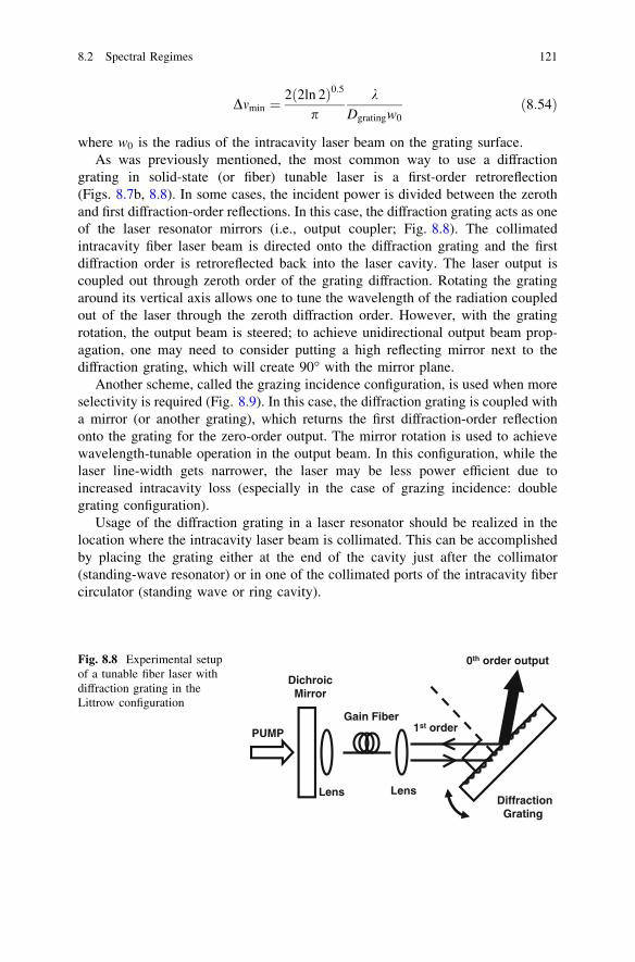
Dmmin ¼2 2ln 2ð Þ0:5

pk

Dgratingw0ð8:54Þ

where w0 is the radius of the intracavity laser beam on the grating surface.As was previously mentioned, the most common way to use a diffraction

grating in solid-state (or fiber) tunable laser is a first-order retroreflection(Figs. 8.7b, 8.8). In some cases, the incident power is divided between the zerothand first diffraction-order reflections. In this case, the diffraction grating acts as oneof the laser resonator mirrors (i.e., output coupler; Fig. 8.8). The collimatedintracavity fiber laser beam is directed onto the diffraction grating and the firstdiffraction order is retroreflected back into the laser cavity. The laser output iscoupled out through zeroth order of the grating diffraction. Rotating the gratingaround its vertical axis allows one to tune the wavelength of the radiation coupledout of the laser through the zeroth diffraction order. However, with the gratingrotation, the output beam is steered; to achieve unidirectional output beam prop-agation, one may need to consider putting a high reflecting mirror next to thediffraction grating, which will create 90� with the mirror plane.

Another scheme, called the grazing incidence configuration, is used when moreselectivity is required (Fig. 8.9). In this case, the diffraction grating is coupled witha mirror (or another grating), which returns the first diffraction-order reflectiononto the grating for the zero-order output. The mirror rotation is used to achievewavelength-tunable operation in the output beam. In this configuration, while thelaser line-width gets narrower, the laser may be less power efficient due toincreased intracavity loss (especially in the case of grazing incidence: doublegrating configuration).

Usage of the diffraction grating in a laser resonator should be realized in thelocation where the intracavity laser beam is collimated. This can be accomplishedby placing the grating either at the end of the cavity just after the collimator(standing-wave resonator) or in one of the collimated ports of the intracavity fibercirculator (standing wave or ring cavity).

PUMP

0th order output

Gain Fiber

Diffraction Grating

LensLens

DichroicMirror

1st order

Fig. 8.8 Experimental setupof a tunable fiber laser withdiffraction grating in theLittrow configuration

8.2 Spectral Regimes 121

8.2.1.2 Prism-Based Tunable Lasers

The simplest and most cost-effective dispersive intracavity laser element is asimple optical prism. Material selection is usually dictated by the spectral range ofoperation and required dispersion, which is proportional to the prism refractiveindex. Fused silica is commonly used for the visible and near-infrared spectralrange, where the highest possible dispersion is not required. In the same spectralrange, prisms made of sapphire, YAG, or flint glass are used for higher dispersion.In the long wavelength range of the optical spectrum (i.e., near or over 3 lm),CaF2 or similar crystals are widely used. In the ultraviolet spectral range, crys-talline quartz is a good choice because it has high transmission in this spectralrange. Because most laser systems are polarized, Brewster angle prisms can beused, which can provide minimal intracavity loss for S polarization. Note that aprism-based intracavity tuning element is one of the most power tolerant becauseits damage threshold is determined only by a surface and bulk damage threshold ofthe prism material, which is very high compared with metallic grating or even anetalon (which has reflective coatings with limited damage threshold; describedlater in this chapter).

Figure 8.10 shows a prism-tuned fiber laser schematic similar to that used byHanna et al. [15]. The design employs a high-dispersion prism set consisting ofthree prisms (for increased dispersion) between a fiber end and feedback mirror(output coupler). The tuning is achieved by angular adjustment of the mirror closeto the prism. If high reflecting mirrors are used on both resonator ends, the outputradiation is coupled through the reflection from one facet of the prism. Note that asimilar dispersive resonator is widely used for tunable solid-state lasers, such asTi3+:sapphire laser.

This section provides some formulas to calculate the prism-based tunable laserline-width. Dispersion of the single prism-based resonator with the prism’s apexangle, which allows the incident light to enter the prism under the Brewstercondition tan HBR ¼ nð Þ on both prism facets, can be calculated by the followingformula:

PUMP

Gain Fiber

Diffraction Grating

LensLens

DichroicMirror

Reflective Mirror

0th order output

1st order

Fig. 8.9 Grazing incidenceconfiguration with awavelength-tuning rotatingmirror

122 8 Main Operating Regimes of Fiber Lasers

Dres ¼ 4dn

dkð8:55Þ

The typical value of the dispersion dn=dkð Þ in visible spectral range for mostprism materials is *0.05 mrad/nm. Then, the full dispersion is Dres = 2 9 10-4

rad/nm.For the prism-based laser resonator, the selective loss spectral distribution of

the resonator has the following bandwidth:

dkres ¼ffiffiffiffiffiffiffiffiffi

Lloss

p hres

Dres

ð8:56Þ

where Lloss is the total nonselective losses of the resonator at the wavelength of thelaser emission and hres is laser divergence. If one assumes klaser ¼ 500 nm, non-selective losses of Lloss ¼ 0:01, and laser divergence of hres ¼ 0:001, then theestimated bandwidth of the laser emission is close to: dkres � 0:5 nm ordmres � 20 cm�1, which obviously points to a not very high selectivity of theprism-based resonator. The wavelength selectivity, however, can be improvedusing a sequence of prisms (Fig. 8.10) or an intracavity prism with a high index ofrefraction.

8.2.1.3 Birefringent Tuning Plates (Lyot Filter)-Based Lasers

The birefringent plate-based intracavity tuning element is another example of ahigh-power tolerant dispersive element. An intracavity wavelength filter of thistype adjusts the wavelength of maximum transmission by rotation of the filter(Fig. 8.11).

Usually, a birefringent plate is cut in such way that its optical axis is in theplane of the plate [16]. Tuning of the wavelength is accomplished by rotation ofthe plate about its normal axes. The birefringent plate needs to be located betweentwo polarizers or the plate has to be oriented at the Brewster angle to the laser

PUMP

Gain Fiber

LensLens

DichroicMirror

Output Coupler

Output

Fig. 8.10 Example of aprism-tuned fiber laserschematic

8.2 Spectral Regimes 123

resonator axis. Multiple plates are used for higher filter selectivity. Each individualplate of the so-called multistage Lyot filter is usually made of crystalline quartz.Each plate’s thickness differs by an integer number.

Basic formulas are presented here to describe the operation of the birefringenttunable filter and its main parameters. For the case of the ring laser resonator(which is very important in fiber lasers), when the plate is inserted into the ringlaser cavity at the Brewster angle ðhBRÞ, sF is defined as a transmission of the S-polarized beam through the plate as follows (assuming the P-polarized beam istransmitted through the plate without loss):

sF ¼2n

n2 þ 1ð Þ ð8:57Þ

where n � no þ neð Þ=2; no þ neð Þ, no=ne are ordinary/extraordinary refractiveindexes. Then, the ring laser resonator transmission band width can be computedas follows:

dmres �2 1� sFð Þ � c

plplate ne � noð Þ

ffiffiffiffiffiffiffiffiffiffiffiffiffiffiffiffiffiffiffiffi

� ln 2ln sF

ffi �

s

ð8:58Þ

where lplate is the plate thickness.Figure 8.12 shows a typical linear tunable fiber laser schematic with a bire-

fringent tunable filter as an intracavity wavelength selective element.A more detailed description of Lyot filters for tunable laser applications can be

found in Hodgkinson and Vukusic [16], Hanna e al. [17] and references therein.

8.2.2 Single Longitudinal Mode Lasers

Longitudinal laser modes (sometimes called axial modes) belong to the frequencydomain of the laser mode structure. While oscillating on a single transverse mode

BR

Resonator Beam

Optical axis of the crystalline

quartz crystal

Rotation direction

of the whole assembly

Normal to the plate’s surface

Fig. 8.11 A typicalthree-stage birefringent filter

124 8 Main Operating Regimes of Fiber Lasers

(TEM00 for open resonators and LP01 for optical fibers) with close to diffraction-limited beam quality, the laser may oscillate at the same time on several longi-tudinal (i.e., spectral) modes.

For a laser with the Fabry–Perot resonator length Lres, spacing of the laserlongitudinal modes is given by:

Dmres ¼c

2nLres

ð8:59Þ

where n is the refractive index of the space between laser cavity mirrors and c is thespeed of light. From this formula, it is clear that the laser resonator mode structure isa sequence of periodic and equidistant discrete frequencies. If the laser gainmedium has a gain band width that is wider than a longitudinal mode separation andthe laser gain is high enough, several longitudinal modes that fall into the laser gainbandwidth have a chance to reach the threshold and participate in laser operation.Oscillation on several longitudinal modes is called multi–longitudinal mode laseroperation.

The number of the longitudinal modes participating in the laser operation canusually be read as a third mode index. For open laser resonators, the general modenotation can be read as:

TEMmnq ð8:60Þ

where q is the longitudinal mode index. The number of oscillating longitudinalmodes in the laser depends on several factors, including (but not limited to)intracavity loss distribution at laser frequencies, length of the laser resonator,pump power, and laser medium gain band. If one is able to reduce the number ofoscillating longitudinal modes to one, the laser starts oscillating on a single lon-gitudinal mode; that is, it becomes a single-frequency (SF) laser.

8.2.2.1 Single-Frequency Laser Operation

In practice, the goal of selecting a single longitudinal mode of laser operation canbe achieved using several effective and well-developed techniques:

PUMP

Gain Fiber

LensLens

DichroicMirror Output Coupler

Output

3-stage Birefringent

Tunable Filter

Fig. 8.12 Birefringent plate(Lyot filter)-based fiber laser

8.2 Spectral Regimes 125

1. Using an intra-cavity Fabry–Perot (FP) etalon, which creates its own trans-mission spectral profile on the background of the laser cavity mode separation andworks as an intracavity axial mode filter.

2. Using a wavelength-dispersive, highly selective laser resonator, which cre-ates high wavelength-dependent cavity losses on frequencies other than thoseselected for laser operation.

3. Using very short laser cavities, in which the laser resonator itself acts as ahighly selective FP etalon (by frequency filter) by introducing increased separationof neighboring longitudinal modes.

4. Seeding a higher power laser by an SF seed laser, which is injection seedingbased on the forced oscillation of slave (i.e., higher power laser, by injecting lowpower, SF master oscillator).

5. Using passive Q-switching, which uses a longer buildup time during passiveQ-switch laser creation compared with that of active Q-switching (longer builduptimes require more laser roundtrips of photons in the cavity, which in turn acts as alongitudinal mode discriminator).

6. Cooling of the laser gain medium, which is especially important in the caseof solid-state lasers, when the gain medium emission spectral bandwidth getsnarrower during cooling (this technique forces reduction of the laser gain band,which in turn reduces the number of longitudinal modes participating in laseraction).

Different techniques are used in different types of lasers and at differentoperational conditions. This section gives a more detailed review of the techniquesthat are more practical and more widely used in fiber lasers.

8.2.2.2 IntraCavity Fabry-Perot Etalon

This technique is an effective method of single longitudinal mode selection in lasersand is widely used in fiber lasers for longitudinal mode selection (or tenability; e.g.,with the scanning FP etalon by Micron Optics).

As mentioned previously, the laser resonator longitudinal mode separation is asfollows:

Dmres ¼c

2nLresð Þ ð8:61Þ

From this expression, one see that a thin intracavity FP etalon with a freespectral range bigger than the laser cavity mode separation can act as an efficientlaser resonator axial mode filter. Here, the basic formulas for the FP etalon aregiven. The FP etalon mode spacing, which is also called the free spectral range(FSR), is determined by the following expression:

DmFSR ¼ FSRetalon ¼c

2netalonLetalon

ð8:62Þ

126 8 Main Operating Regimes of Fiber Lasers

where netalon is the refractive index of the material between etalon reflectingsurfaces and Letalon is the distance between etalon reflecting surfaces (or base of theetalon). Another important parameter of the FP etalon is its finesse. For a loss-freeetalon, finesse is determined by:

Fetalon ¼p R1R2ð Þ1=4

1�ffiffiffiffiffiffiffiffiffiffiffiffiffiffi

R1R2ð Þp ð8:63Þ

The finesse indicates how much narrower the transmission peak of the etalon isthan the spectral separation between neighboring transmission peaks (i.e., FSR).

One can deduce accordingly that individual transmission peak of the FP etalonhas the following spectral width:

Dmpeak ¼FSRetalon

Fetalon

ð8:64Þ

As a rule of thumb to achieve a single longitudinal mode operation of the laser,the etalon FSRetalon should be wider than the laser medium-gain band. It alsorequires that FSR of the intracavity FP etalon is wider than the distance betweenthe neighboring frequency modes of the laser resonator.

In an interesting case of so-called microchip lasers, the laser cavity itself is veryshort and acts as a laser resonator and FP longitudinal mode filter. Such lasers wereproposed in the late 1980s and were based mostly on existing solid-state lasermaterials such as Nd:YVO4, in which a high concentration of active ions allowefficient pump power absorption in a thickness of millimeter and submillimeterscales. With laser mirrors directly created on such thin crystal surfaces, the wholelaser might be less than 1 mm thick and favorable conditions for SF oscillation arereadily available. Microchip laser geometry is difficult to realize in the case of fiberlasers because of the long length of the fiber laser-active medium. However, SFmicrochip solid-state lasers can be used (and are used) as a master oscillators orseeds in high-power fiber laser MOPA systems.

Another widely used technique to achieve single-frequency oscillation in fiberlasers is based on the development of so-called fiber Bragg gratings (FBGs). FBGscan be directly written into the single-mode doped fiber core by recording a pictureof periodical change of the core refractive index using an ultraviolet laser. Such apicture is a result of the interaction between two coherent ultraviolet laser beams,usually after a split of a single laser, that are then redirected to create an inter-ference pattern on the fiber.

The fundamental physical principle behind FBG is Bragg reflection. When lighttravels through the region of periodically alternative regions of high and lowrefractive indexes, it is partly reflected at each index step. If the distance betweenthe low and high index of refraction allows all the reflected light waves to add inphase, then the integrated reflection grows up significantly. This in-phasereflecting condition can be satisfied for certain wavelengths and is possible whenthe doubled distance between two reflections (grating period; i.e., the distance

8.2 Spectral Regimes 127

between the low and high refractive index areas) is equal to an integral number ofpropagating light wavelengths:

kB ¼ 2nK and LFBG ¼ NK ð8:65Þ

where K is the grating period, N is the number of the FBG refractive index periodicvariations, and and LFBG is the FBG length.

It is useful here to give basic formulas for the calculation of the main param-eters of FBG. There are two main parameters in the design of FBG and itsapplications: FBG reflectivity and FBG spectral bandwidth. The FBG reflectivitycan be computed using the following expression [18, 19]:

RFBG ¼ tan h2 pdnLFBG

kB

ffi �

ð8:66Þ

where dn is the refractive index variation along the grating period.The FBG spectral bandwidth can be expressed using following relationship:

DkFBG ¼2dn

p

ffi �

kB ð8:67Þ

FBGs act as reflectors, and a couple of them inside the laser cavity can create anFP intracavity etalon. On the other hand, narrow spectral band reflective FBGs,used as a laser cavity mirror along with short gain fiber, allow the achievement ofthe single longitudinal operation of the fiber lasers. Figure 8.13 shows an exampleof SF fiber lasers using FBGs as a narrowband output coupler.

Another effective use of FBGs for SF fiber laser operation is a so-called dis-tributed feedback (DFB) linear laser configuration. In this type of SF fiber laser,the Bragg grating is written into (or close to) the core of the gain fiber. Forachieving single-sided output, the FBG was written on the fiber by offsetting thephase shift from the center position by half a grating period [20]. Single polari-zation is achieved by creating the phase-shifted FBG with ultraviolet lightpolarized perpendicular to the propagation axes of the gain fiber by forcing lightphotons with certain polarization states to be coupled into the waveguide. Usingsuch an approach, researchers [21] achieved [20 mW of unidirectional and singlepolarization (PER *40 dB) fiber laser output.

Single-frequency lasers are widely used in science and technology for differentapplications, from optical communications and nonlinear optics to sensors ofdifferent types.

8.2.2.3 Minimum Line-Width of the Laser

When lasers operate on a single longitudinal mode, the minimum laser line-widthis determined by the spontaneous emission noise. This is valid for gas and mosttypes of solid-state lasers. Based on a semi-classical approach, the following

128 8 Main Operating Regimes of Fiber Lasers

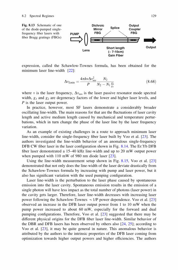
expression, called the Schawlow-Townes formula, has been obtained for theminimum laser line-width [22]:

DmLmin ¼4phmDm2

res

P

N2

N2 � N1g2g1

ð8:68Þ

where m is the laser frequency, Dmres is the laser passive resonator mode spectralwidth, g1 and g2 are degeneracy factors of the lower and higher laser levels, andP is the laser output power.

In practice, however, most SF lasers demonstrate a considerably broaderoscillating line-width. The main reasons for that are the fluctuations of laser cavitylength and active medium length caused by mechanical and temperature pertur-bations, which in turn change the phase of the laser line by the laser frequencyvariation.

As an example of existing challenges in a route to approach minimum laserline-width, consider the single-frequency fiber laser built by Voo et al. [23]. Theauthors investigated the line-width behavior of an anomalous single-frequencyDFB CW fiber laser in the laser configuration shown in Fig. 8.14. The Er:Yb DFBfiber laser demonstrated a 15–40 kHz line-width and up to 20 mW output powerwhen pumped with 110 mW of 980 nm diode laser [23].

Using the line-width measurement setup shown in Fig. 8.15, Voo et al. [23]demonstrated that not only does the line-width of the laser deviate drastically fromthe Schawlow-Townes formula by increasing with pump and laser power, but italso has significant variation with the used pumping configuration.

Laser line-width is the perturbation to the laser phase caused by spontaneousemission into the laser cavity. Spontaneous emission results in the emission of asingle photon will have less impact as the total number of photons (laser power) inthe cavity gets larger. Therefore, laser line-width decreases with increasing laserpower following the Schawlow-Townes *1/P power dependence. Voo et al. [23]observed an increase in the DFB laser output power from 1 to 10 mW when thepump power increased to about 60 mW, especially for the forward and dualpumping configurations. Therefore, Voo et al. [23] suggested that there may bedifferent physical origins for the DFB fiber laser line-width. Similar behavior ofthe DBR and DFB lasers has been observed by others also [24, 25]; according toVoo et al. [23], it may be quite general in nature. This anomalous behavior isattributed by the authors to the intrinsic properties of the DFB laser coming fromoptimization towards higher output powers and higher efficiencies. The authors

PUMP

Short length (~ 7-10cm) Gain Fiber

Lens

DichroicMirrorFBG

Output

Output Coupler

FBG

SpliceFig. 8.13 Schematic of oneof the diode-pumped single-frequency fiber lasers withfiber Bragg gratings (FBGs)

8.2 Spectral Regimes 129

suggest that the master oscillator-power amplifier configuration is expected toproduce better results in terms of line-width.

In pulsed laser systems, the laser spectral line limit is determined by theso-called transform limited condition. For Gaussian pulses, this condition can beexpressed as follows:

DmLlim tp � 0:44 ð8:69Þ

where tp is the laser pulse width. It is assumed that the pulse is Chirp free.

Fig. 8.14 Distributed feedback (DFB) fiber laser pumping configurations: a backward (counter)pumping, b forward (co-) pumping, and c dual side pumping schemes [23] (Image courtesy ofSPIE)

Fig. 8.15 Experimental setup for line-width measurement using a delayed self-heterodynetechnique [23]. DFB, distributed feedback (Image courtesy of SPIE)

130 8 Main Operating Regimes of Fiber Lasers

References

1. R.W. Hellwarth, Control of fluorescent pulsations, in Advances in Quantum Electronics, ed.by J.R. Singer (Columbia University Press, New York, 1961), pp. 334–341

2. W.G. Wagner, B.A. Lengyel, Evaluation of the giant pulse in a laser. J. Appl. Phys. 34(7),2040–2046 (1963)

3. W. Koechner, Solid-State Laser Engineering, 5th edn. (Springer, Berlin, 1999), p. 7464. A.V. Smith, B.T. Do, Bulk and surface laser damage of silica by picosecond and nanosecond

pulses at 1064 nm. Appl. Opt. 47(26), 418–4832 (2008)5. F.Y. Génin, A. Salleo, T.V. Pistor, L.L. Chase, Role of light intensification by cracks in

optical breakdown on surfaces. J. Opt. Soc. Am. A: 18, 2607–2616 (2001)6. Z.J. Chen, A.B. Grudinin, J. Porta, J.D. Minelly, Enhanced Q switching in double-clad fiber

lasers. Opt. Lett. 23, 454–456 (1998)7. A.M. Ratner, Spectral, Spatial, and Temporal Properties of Lasers (Plenum Press, New York,

1972), pp. 1–2208. D.J. Kuizenga, A.E. Siegman, FM and AM mode locking of the homogeneous laser—Part I:

Theory. IEEE J. Quantum Electron. 6(11), 694–708 (1970)9. A. Siegman, Lasers (University Science books, USA, 1986), p. 1283

10. H. Statz, G.A. deMars, Quantum Electronics, ed. by C.H. Townes (Columbia UniversityPress, New York, 1960), p. 530

11. O. Svelto, Principles of Lasers, 4th edn. (Plenum Press, New York, 1998), p. 60512. D.H. Gill, B.E. Newnam, Picosecond-pulse damage studies of diffraction gratings, in

Damage in Laser Materials, vol. 727, ed. by H.E. Bennett, A.H. Guenther, D. Milam, B.E.Newnam (National Bureau of Standards Special Publication, USA, 1986), pp. 154–161

13. E.G. Loewen, E. Popov, Diffraction Gratings and Applications (Marcel Dekker, Inc., NewYork, 1997), p. 485

14. C.A. Huguley, J.S. Loomis, Optical material damage from 10.6 lm CW radiation, in Damagein Laser Materials, vol. 435, ed. by A.J. Glass, A.H. Guenther (National Bureau of StandardsSpecial Publication, USA, 1975)

15. D.C. Hanna, R.M. Percival, I.R. Perry, R.G. Smart, P.J. Suni, A.C. Tropper, An Ytterbium-doped monomode fibre laser: broadly tunable operation from 1.010 lm to 1.162 lm andthree level operation at 974 nm. J. Mod. Opt. 37(4), 517–525 (1990)

16. I.J. Hodgkinson, J.I. Vukusic, Birefringent filters for tuning flashlamp-pumped dye lasers:simplified theory and design (T). Appl. Opt. 17, 1944–1948 (1978)

17. D.C. Hanna, R.M. Percival, R.G. Smart, A.C. Tropper, Efficient and tunable operation of aTm3þ-doped fibre laser. Opt. Commun. 75, 283–286 (1989)

18. T. Erdogan, Fiber grating spectra. J. Lightwave Technol. 15, 1227–1294 (1997)19. A. Othonos, K. Kalli, FBG: Fundamentals and Applications in Telecommunications and

Sensing (Artech House, Boston, 1999). Chapter 520. V.C. Lauridsen et al., Design of DFB fiber lasers, in Proceedings of ECOC, vol. 3,

(Edinburgh, UK, 1997), pp. 39–4221. M. Ibsen et al., Robust high power ([ 20 mW) all-fiber DFB lasers with unidirectional and

truly single polarization outputs, Conference Proceedings, CLEO’ 99, (Wasgington DC,OSA, 1999), pp. 245–246

22. A.L. Schawlow, C.H. Townes, Infrared and optical masers. Phys. Rev. 112, 1940–1949(1958)

23. N.Y. Voo, P. Horak, M. Ibsen, W.H. Loh, Linewidth and phase noise characteristics of DFBfibre lasers, in Proceedings SPIE, vol. 5620, 2004, Solid State Laser Technologies andFemtosecond Phenomena, eds. by Jonathan A. C. Terry; W. Andrew Clarkson, pp. 179–186

24. NP Photonics, Scorpion’ Laser Module, Product Data Sheet Rev 4. Available at: http://www.npphotonics.com/files/Laser_Module.pdf

25. W.H. Loh, S.D. Butterworth, W.A. Clarkson, Efficient distributed feedback erbium-dopedgermanosilicate fiber laser pumped in the 520 nm band. Electron. Lett. 32, 2088–2089 (1996)

References 131

26. Y. Gan, W.H. Xiang, G.Z. Zhang, Studies on ytterbium-doped fibre laser operating indifferent regime. J. Phys: Conf. Ser. 48, 795–799 (2006)

27. L. Reekie, R.J. Mears, S.B. Poole, D.N. Payne, Tunable single-mode fiber lasers. IEEE J.Lightwave Technol. 4(7), 956–960 (1986)

28. K.R. German, Grazing angle tuner for CW lasers. Appl. Opt. 20, 3168–3171 (1981)29. J.T. Kringlebotn, P.R. Morkel, L. Reekie, J.L. Archambault, D.N. Payne, Efficient diode-

pumped single-frequency erbium: ytterbium fibre laser. IEEE Photonics Technol. Lett. 5(10),1162–1164 (1993)

132 8 Main Operating Regimes of Fiber Lasers

Chapter 9Main Optical Components for FiberLaser/Amplifier Design

9.1 Laser Diodes

9.1.1 Principles of Operation

The first reported theoretical analysis and prediction of laser action based on asemiconductor diode was published in 1959 in the USSR [1]. The first operation ofa semiconductor laser (also called a ‘‘diode laser’’ or ‘‘laser diode’’) was reportedin 1962 in the USA [2]. Semiconductor lasers play a very important role in thefiber laser field. Therefore, this section provides a detailed description of thephysical processes that take place in these laser devices.

Unlike isolated atoms and molecules (and even some laser optical centers indoped dielectrics), semiconductors demonstrate wide energy bands. These bandsare separated by a bandgap (Fig. 9.1). Typical values of the bandgap of semi-conductor materials for the most commonly used and commercially availablediode lasers are on the order of a few electron volts. Under certain excitationconditions, such as injecting an electrical current, optical excitation, or heating,electrons from the valence band can move from the valence band to the conductionband after absorbing energy by an excitation process. As a result of this interbandelectron transition, a pair of charge carriers can be created (i.e., electrons in theconduction band and holes in the valence band), which is called an electron–holepair. If an electron undergoes reverse transition (i.e., from the conduction band tothe valence band), the process is called electron–hole recombination. The result ofthis interband recombination is usually an extraction of energy that was receivedduring the excitation process.

In equilibrium, electron–hole pairs can be created and recombined as a result ofthermal diffusion and spontaneous emission of photons. Thermal equilibrium ofelectrons and holes, in this case, produces a certain concentration of electrons inthe conduction band and holes in the valence band. Note that electrons are fer-mions (their spin equals 1/2) and thus follow so-called Fermi–Dirac statistics.Therefore, a probability of the electron occupying a certain level with energy E at

V. Ter-Mikirtychev, Fundamentals of Fiber Lasers and Fiber Amplifiers,Springer Series in Optical Sciences 181, DOI: 10.1007/978-3-319-02338-0_9,� Springer International Publishing Switzerland 2014

133

temperature T in either the conduction or valence band is described by thefollowing Fermi–Dirac formula:

fF�DðE; TÞ ¼1

1þ exp E�EF

kT

h i ð9:1Þ

where T is the absolute temperature, EF is the Fermi energy, and k is the Boltz-mann constant. The Fermi energy EF (and, associated with it, the Fermi level in asemiconductor) is an energy that corresponds to the highest energy state occupiedby a carrier (either an electron or hole; Fig 9.1). The Fermi level and Fermi energyplay a very important role in the physics of the semiconductor lasers, particularlyin the creation of the population inversion.

In equilibrium, the number of electrons in the valence band is essentially higherthan in the conduction band; therefore, absorption of light during excitation is amajor process for interband transitions. If, however, one creates a condition whereelectrons occupy the majority of levels at the bottom of the conduction band andholes occupy most levels at the top of the valence band, such a condition is called adegenerate condition or a degenerate state. In degenerate semiconductors, emis-sion processes will dominate the absorption. To create a population inversioncondition, one must fill more than half of the levels in the band of the order ofkT near the band’s edge with electrons (in the conduction band) and holes (in thevalence band).

In the theory of semiconductor lasers, the condition of population inversion isexpressed in terms of Fermi energy for electrons in the conduction band and holesin the valence band. As mentioned above, Fermi energy defines the energy levelwith the highest energy that can be occupied by an electron. The probability of theelectron to occupy Fermi level is given by:

fF�DðEe; TÞe ¼1

1þ exp Ee�EFe

kT

h i ð9:2Þ

Fig. 9.1 Energy spectrum ofthe degenerate semiconductor

134 9 Main Optical Components for Fiber Laser/Amplifier Design

where EFe is the Fermi energy of the electron. With increasing electron concen-tration in the conduction band, the Fermi energy of the electron increases;therefore, electron degeneracy increases as well (Fig. 9.1).

Similarly, the probability for holes to occupy energy levels in the valence canbe determined as follows:

fF�DðEh; TÞh ¼1

1þ exp EFh�Eh

kT

h i ð9:3Þ

where EFh is the Fermi energy for holes. Note that:

fF�D Eh; Tð Þh¼ 1� fF�D Ee; Tð Þe ð9:4Þ

If the semiconductor material demonstrates the degenerate state for bothelectrons and holes, then the energy gap between Fermi energy for electrons andFermi energy for holes exceeds the bandgap of the material:

EFe � EFh [ Eg ð9:5Þ

This condition in turn is required for amplification of light in a semiconductorand basically defines the condition of population inversion.

There are several ways to create a condition of inversion population in semi-conductors: namely, optical pumping, excitation with an electron beam, andinjection of carriers through the p-n junction of the semiconductor. Carrierinjection through a p-n junction is the most popular option; this section describesits use to create the required conditions for amplification and oscillation insemiconductors. Because the first diode laser was based on a single GaAs crystal,an example of a semiconductor laser based on this material and physical processesleading to the laser action are reviewed here.

Consider a GaAs crystal doped with Zn. The dopant creates an energy levelwithin the bandgap close to the top of the valence band (Fig 9.2b). Electronstraveling in the valence band need little thermal energy kT (kT is *0.025 eV at300 K, while the bandgap of GaAs is *1.4 eV) to jump into the above-mentionedenergy level, leaving behind positively charged holes (Fig 9.2b). In this case, theimpurity level is called an acceptor level because an electron is accepted to thislevel.

As a result, a created hole can work as a trap for another electron still travelingin the valence band. Once trapped by this hole, the valence band propagating theelectron leaves another hole behind. In this way, one can consider holes movingaround in the valence band. The moving hole becomes a carrier of charge, and thematerial now becomes a p-type semiconductor (Fig. 9.2b). In a p-type semicon-ductor, holes are considered majority carriers.

On the other hand, if the same GaAs material is doped with Si, the impuritycreates an energy level in the bandgap; in this case, it is very close to the bottom ofthe conduction band. With similar considerations as mentioned above, an impurityelectron occupying an energy level in the bandgap very close to the conduction

9.1 Laser Diodes 135

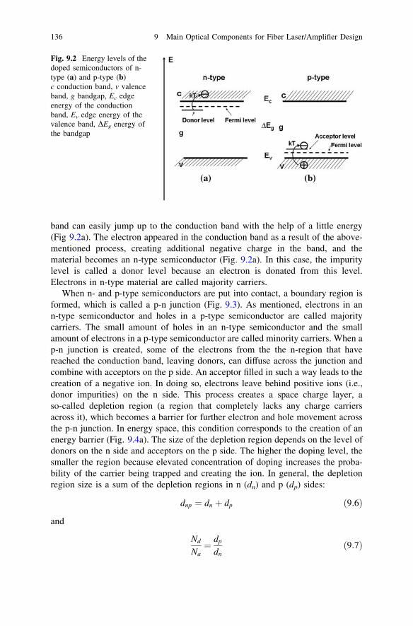
band can easily jump up to the conduction band with the help of a little energy(Fig 9.2a). The electron appeared in the conduction band as a result of the above-mentioned process, creating additional negative charge in the band, and thematerial becomes an n-type semiconductor (Fig. 9.2a). In this case, the impuritylevel is called a donor level because an electron is donated from this level.Electrons in n-type material are called majority carriers.

When n- and p-type semiconductors are put into contact, a boundary region isformed, which is called a p-n junction (Fig. 9.3). As mentioned, electrons in ann-type semiconductor and holes in a p-type semiconductor are called majoritycarriers. The small amount of holes in an n-type semiconductor and the smallamount of electrons in a p-type semiconductor are called minority carriers. When ap-n junction is created, some of the electrons from the the n-region that havereached the conduction band, leaving donors, can diffuse across the junction andcombine with acceptors on the p side. An acceptor filled in such a way leads to thecreation of a negative ion. In doing so, electrons leave behind positive ions (i.e.,donor impurities) on the n side. This process creates a space charge layer, aso-called depletion region (a region that completely lacks any charge carriersacross it), which becomes a barrier for further electron and hole movement acrossthe p-n junction. In energy space, this condition corresponds to the creation of anenergy barrier (Fig. 9.4a). The size of the depletion region depends on the level ofdonors on the n side and acceptors on the p side. The higher the doping level, thesmaller the region because elevated concentration of doping increases the proba-bility of the carrier being trapped and creating the ion. In general, the depletionregion size is a sum of the depletion regions in n (dn) and p (dp) sides:

dnp ¼ dn þ dp ð9:6Þ

and

Nd

Na¼ dp

dnð9:7Þ

Fig. 9.2 Energy levels of thedoped semiconductors of n-type (a) and p-type (b)c conduction band, v valenceband, g bandgap, Ec edgeenergy of the conductionband, Ev edge energy of thevalence band, DEg energy ofthe bandgap

136 9 Main Optical Components for Fiber Laser/Amplifier Design

where Nd and Na are concentrations of donors and acceptors, respectively. Ifdoping level of the p-type side is higher than the n-type side (i.e., Nd \ Na), thendn [ dp; that is, the depletion region mostly occupies the n-type of the semicon-ductor. The typical size of the depletion region is on the order of a fraction of themicron (i.e., *0.1, *0.4 lm for doping density *1016 cm-3) [3].

If one applies an external electric field or so-called forward bias (forwardvoltage) across the p-n junction (positive to p-type and negative to n-type), it cancreate an additional amount of electrons following the appearance of electricalfield (i.e., injected) at the n-side and holes at the p-side of the junction (Fig 9.4b).Basically, the necessary voltage (the bias voltage) is required to overcome apotential barrier created in the depletion region. As one can see from Fig. 9.4,applying forward voltage reduces the existing energy barrier. The forward voltagerequired to overcome the energy barrier of the p-n junction is very close to the

Fig. 9.3 Depletion region inthe junction area of n-typeand p-type semiconductors

Fig. 9.4 Energy banddiagram for a p-n junction:(a) V = 0; (b) V [ 0. EFe andEFh, Fermi energies forelectrons and holes,respectively

9.1 Laser Diodes 137

energy of the bandgap and is on the order of 1–2 V (for visible and infrared diodelasers). Note that when no forward voltage is applied, the two Fermi levels arealigned (Fig 9.4a). However, when the forward voltage is applied, the Fermi levelsbecome separated by a value close to eV and the energy barrier for the carriers getssmaller. In the condition of applied forward voltage, electrons can more easilypenetrate into the p-type side. During diffusion, the electron penetration depth intop-type material (i.e., a length; the carrier defuses before recombination), which iscalled a minority diffusion length, can be determined by the following formula:

dM ¼ffiffiffiffiffiffiffiffiffiffiffiffiffiffiffiffiffiffi

DM � sM

pð9:8Þ

where DM is the bulk minority diffusion coefficient (for GaAs, DM = 10 cm2/s)and sM (for GaAs, sM = 1 ns) is the lifetime (i.e., minority carrier recombinationtime) [4]. Calculated this way, penetration distance is *1 lm. This distancedetermines the laser-active region in a semiconductor laser in the direction per-pendicular to the plane of junction.

Injected electrons into the p-type and injected holes into the n-type of thesemiconductor boundary can recombine and in such a way emit a light with photonenergy roughly corresponding to the bandgap of the semiconductor material. If onethen creates a resonator (usually two cleaves perpendicular to the plane of thejunction), this may bring the system to the threshold condition, where gain due tothe stimulated emission from carrier recombination overcomes losses. The currentrequired to achieve the lasing threshold is called the threshold current (Fig. 9.6)and is a very important parameter of the semiconductor laser. This is the basicprinciple of semiconductor laser operation and in fact describes the first semi-conductor lasers based on GaAs single crystals (Fig. 9.5). Such a semiconductorlaser type is also called a homojunction laser, in which both n-type and p-typesemiconductors are made of the same material. Also described was an injectiontype of pumping for semiconductor lasers. Other pumping architectures have beensuggested, including optical pumping and electron beam pumping approaches.

Fig. 9.5 Configuration of theedge-emitting semiconductorlaser [12] (Image courtesy ofthe OpticalSociety ofAmerica)

138 9 Main Optical Components for Fiber Laser/Amplifier Design

However, among the commercially available and most widely used diode lasers,injection lasers are widely used, especially as pump sources of fiber lasers andamplifiers.

One of the biggest problems in the operation of early diode lasers was heating,which in turn prevented room-temperature continuous-wave (CW) operation. Toovercome this problem, an interesting method was suggested, which consisted ofcreating a suitable multilayered crystal of GaAs and AlGaAs. Variation in electricaland optical properties in the multilayered crystal required replacement of a largefraction of the Ga. Technological development continued in this direction in orderto maintain no sizing defects in the interfaces between the layers, as caused by sizematch of the crystal lattices. This eventually lead to the creation of so-calledheterostructure diode lasers, which allowed CW operation at room temperature.After this important discovery, the field of diode lasers grew dramatically. Thefollowing section reviews the most widely used types of diode lasers.

Figure 9.6 shows the typical function of the diode laser’s output power versuspump current. Note that the diode laser’s output power pump dependence curvehas a rollover area, which is called a kink. This kink arises from local overheatingof the chip at high pump current and should be avoided. Usually diode lasermanufacturers specify a so-called kink-free operation, which is typically definedby a distance from the kink in current values. Working in a kink-free pump currentzone prolongs the diode laser’s lifetime.

9.1.1.1 Metal–Organic Vapor Deposition for Diode Laser ChipFabrication

Several techniques have been developed for semiconductor laser material manu-facturing. One of the most commonly used techniques for thin-film deposition andhigh-quality crystalline chip manufacturing is metal–organic vapor deposition

Fig. 9.6 General view of theoutput power versus pumpcurrent function for the diodelaser

9.1 Laser Diodes 139

(MOCVD) or its variations. MOCVD is popular for several reasons, including itsexcellent thickness control, possibility to grow numerous thin (*1 nm) layers ofcomplex heterostructures, good uniformity of growth structures, capabilities ofpatterned (i.e., localized) growth, and scalability for large area-multiple wafergrowth. In addition, the MOCVD technique demonstrates high growth yield.

MOCVD uses a process of epitaxial growth, which in turn consists of depos-iting thin layers of material at a desired thickness and molecular composition. Thegeneral schematic of the MOCVD process is illustrated in Fig. 9.7.

For the case of GaAs-based diode laser structures, the GaAs substrate in theform of a thin disk 50–90 mm in diameter (a wafer) is placed in a reactionchamber, heated up to temperatures of 600–1100 �C (see Fig. 9.7). During theMOCVD process, source materials through mass flow control and pressure controlare thermally deposited in the reaction chamber; the semiconductor material growsepitaxially on the wafer and creates crystalline layers from the gaseous phase. TheSiO2 insulation layer is deposited and contact structuring is created, then bothsides of the chip are gold coated for electrical connection. The wafer is cleavedinto bars and diode laser cavity mirrors are then deposited. The created bar is thensoldered onto a copper heatsink (which later acts as an electrode or ground). Thewired chip is then packaged into different packaging configurations, includinghermetically sealed systems. For better thermal management (especially in the

Fig. 9.7 a Schematic of the MOCVD technique. b The main steps in a simple GaAs-based diodelaser emitter/bar manufacturing process

140 9 Main Optical Components for Fiber Laser/Amplifier Design

case of high-power diodes), the p-side of the chip is heatsinked and a wire isattached to the opposite side (i.e., the top of the structure that consequentlybecomes a negative electrode; attached to n-type of the semiconductor). Packageddiode lasers may later be fiber coupled (see details later in this chapter).

9.1.2 Main Types of Diode Lasers Used in Fiber LaserTechnology

The most common semiconductors used in laser diodes are compounds based ongallium arsenide, indium gallium arsenide, phosphide, and gallium nitride.Table 9.1 shows most commonly used semiconductor laser compounds and relatedwavelengths of operation in applications for diode pumping of fiber lasers and fiberamplifiers.

9.1.2.1 Basic Structure of Diode Lasers (Single Emitters)

Fabry–Perot Lasers

In the simplest form of the laser diode, an optical waveguide is made on the crystalsurface in such a way that the light is confined to a relatively narrow line. The twoends of the crystal are cleaved to form perfectly smooth, parallel edges, thusforming a Fabry–Perot (FP) resonator with semiconductor gain material locatedbetween reflecting surfaces. Light in the laser diode travels along the waveguidecreated by the p-n junction and is reflected from the end faces of the semicon-ductor. Because one end of the semiconductor material is cleaved the travelinglight inside the diode, the laser cavity undergoes incomplete reflection from thisend facet and emerges outside the diode laser resonator. When the laser thresholdis reached (i.e., when more amplification than loss is achieved), the diode laserbegins to oscillate.

In most types of diode lasers (edge-emitting lasers), the light is confined in avery thin layer—a waveguide. This waveguide is usually supports only a singleoptical mode in one direction (i.e., in the direction perpendicular to the semi-conductor layers or the plane of junction). In this direction, therefore, the diode

Table 9.1 Main types ofdiode laser matrixes andrelated wavelengths ofoperation

Semiconductor compounds Wavelength of operation (nm)

AlGaInP *630–690InGaAlAs/GaAlAs *780–880InGaAs *900–1200InGaAsP/InP *1400–1850InGaAsSb *2000–2200

9.1 Laser Diodes 141

laser beam is close to diffraction limited. In the perpendicular direction, if thewaveguide is wide compared to the wavelength of light, the laser is multimode. Inthis case, due to diffraction, the beam diverges rapidly after leaving the semi-conductor chip, typically at *40� vertically (fast axes) by *10� laterally (slowaxes). The typical wavelength temperature dependence is *0.3 nm/�C. If the laserdiode emitting area is strongly asymmetric, the diode laser is called a broad-arealaser (BAL); this is the case for multimode edge-emitting diode lasers.

The wavelength emitted by a diode laser is a function of the bandgap of thesemiconductor and the modes of the optical cavity. In the laboratory environmentand product installations, spectral properties of the semiconductor laser depend ontemperature and pump current (in the case of injection lasers).

9.1.2.2 Distributed Feedback Lasers and Distributed Bragg ReflectorLasers

Distributed feedback lasers (DFB) are one of the most important type of singleemitter diode lasers used in the field of fiber lasers. This type of diode laser is oftenused as a seed source in high-power fiber amplifiers. To stabilize the lasingwavelength, a diffraction grating is etched close to the p-n junction of the diode(Fig. 9.8). This grating acts like an optical filter, causing a single wavelength to befed back to the gain region; therefore, it affects the laser spectral parameters.Because the distributed feedback (i.e., grating) provides the feedback that isrequired for lasing, reflection from the facets is not required. Therefore, usuallyone facet of a DFB diode laser is antireflection coated.

The DFB laser has a stable wavelength that is set during manufacturing by thepitch of the grating; it can only be tuned slightly with temperature (usually*0.06 nm/K) or by pump current (usually *0.007 nm/mA). DFB diode lasersoperate on a single longitudinal mode with extremely narrow spectral line width ofless than 1 MHz. DFB diode lasers are very sensitive to optical feedback; there-fore, they are usually manufactured with an optical isolator in between thesemiconductor chip and fiber where the laser is coupled (in the case of fiber-coupled devices).

In distributed Bragg reflector (DBR) diode lasers, as with DFB lasers, a Bragggrating is integrated into the diode (Fig. 9.9). However, instead of being etchedinto the gain medium of the chip, the grating is positioned outside the active region

Fig. 9.8 Distributedfeedback (DFB) diode laserstructure (Image courtesy ofSacher Lasetechnik)

142 9 Main Optical Components for Fiber Laser/Amplifier Design

of the cavity. The grating acts as a mirror and reflects a single wavelength backinto the cavity. The rear facet of the laser chip has a high reflection coating,whereas the front facet has an antireflection coating. In some configurations ofDBR lasers, it is possible to provide individual control of the different semicon-ductor chip sections. This in turn allows the achievement of certain flexibility inelectrical modulation of the laser. The laser wavelength tunability of the DBR laseris achieved by synchronously changing the current of the Bragg and the phasesection of the laser.

Both DFB and DBR diode lasers (similar to other diode lasers) are wavelengthtunable with current and temperature. Thermally tuned DFB and DBR lasers havevery large mode-hop free tuning ranges, which can span over hundreds ofgigahertz.

9.1.2.3 Vertical Cavity Surface-Emitting Semiconductor Lasers

Vertical cavity surface-emitting lasers (VCSELs) have their optical cavity axisalong the direction of current flow (i.e., perpendicular to the plane of junction)rather than perpendicular to the current flow as in conventional edge-emitting laserdiodes (described previously). The active region length is very short comparedwith the lateral dimensions (Fig. 9.10). The VCSEL laser resonator consists of two

Fig. 9.9 Distributed Braggreflector diode laser structure(Image courtesy of SacherLasetechnik)

Fig. 9.10 Vertical cavitysurface-emitting laser(VCSEL) structure. DBRdistributed Bragg reflector

9.1 Laser Diodes 143

DBR mirrors parallel to the wafer surface, with an active layer consisting of one ormore quantum wells of semiconductor laser-active material. The planar DBRmirrors consist of layers with alternating high and low refractive indices, creatingboth a high reflector and an output coupler. VCSELs have better wavelengthstability, reduced temperature wavelength dependence (\0.1 nm/C), improvedreliability due to the higher light intensity of the edge versus the surface geometry,and higher temperature of operation ([70 �C). Commercially available high-power VCSELs (i.e., Princeton Photonics) demonstrate more than 1 kW of opticalpower from the 1 mm core (0.4 NA at 975 nm).

Having relatively large mirror surfaces, dielectric mirrors may be fabricatedwith a high degree of wavelength-selective reflectance using a multilayer coatingstructure. Because of the possible high mirror reflectivity, VCSELs have loweroutput powers when compared to edge-emitting lasers. The main advantage of aVSCEL is its round beam shape (compared with the highly astigmatic beamemerging from edge-emitting laser diodes) and convenience of the laser inspectionduring fabrication. Because of their round beam structure, VCSELs also allowresonator geometries and structures that are similar to conventional solid-statelasers, along with similar thermal lensing issues and challenges concerning laserresonator stability. Because the laser resonator axis is in the same direction as thepumping current flow, the shape, size, and structure of the electrodes are essential.

9.1.3 High-Power Diode Lasers

Commercial production and development of laser diodes has been significant sincethe early 1990s. One of the biggest interests is in their power scaling. BALsbecame a focus of the commercial development of high-power diode lasers.Mainly, the diode laser power scaling included single-emitter strip-diode lasers,bars (linear arrays of single emitters), and stacks of such broad-area diode laserstructures. Thus, the principal scaling roadmap is straightforward.

9.1.3.1 Single Emitters

The typically single-emitter BAL layer structure has *1 lm dimension in thedirection perpendicular to the plane of junction (single transverse mode, diffrac-tion-limited propagation) and typically 50–200 lm dimension along the plane ofjunction (i.e., multitransverse mode propagation; see Fig. 9.11). The edge-emittinglaser cavity is about *500 lm. For comparison, the VCSEL laser cavity is typ-ically a few micrometers long.

The wider the multimode dimension of the BAL, the higher is the power that isachievable from the single emitter. (However, there is a limitation related to theonset of the ASE process and parasitic lasing in transverse direction.) Powerscaling of a single-emitter BAL is limited by *5 MW/cm2, mainly because of the

144 9 Main Optical Components for Fiber Laser/Amplifier Design

facet damage; therefore, it allows a 1 9 100 lm laser strip to withhold an opticalpower of typically *3–5 W.

9.1.3.2 Diode Laser Linear Array (Bar)

Numerous applications, ranging from material processing to diode pumping ofsolid-state lasers, drive scientists and engineers to develop more powerful single-emitter BALs. However, straightforward power scaling of diode lasers is limitedby the high power density of the diode laser chip front facet, which in turnproduces a large thermal load and risks a diode chip failure.

Another way to scale the diode laser power is to create single-emitter lineararrays with stable and reliable performance of the individual multimode emitter.Diode arrays are created by linearly aligning a number of single diode laseremitters (during the chip manufacturing process) as a one-dimensional array ofBALs (Fig. 9.12). They typically contain between 19 and 50 emitters, each being*100–200 lm wide. A typical diode laser bar has a laser resonator length ofapproximately a millimeter, a 10 mm width, and has 10 9 40� of divergence atfull-width half-maximum (FWHM) in the slow direction (plane of junction:multimode operation) and fast direction (perpendicular to the plane of junction:single mode, diffraction-limited operation).

Diode laser bars generate tens of watts of output power (typically 20–50 W).The power of a diode laser array depends on the wavelength, chip structure,cooling configuration, and the mode of operation. The most challenging opera-tional mode is CW because, at 100 % duty circle, the heat load on the chip istremendous at a high power level of operation. Currently, the most powerful CWdiode laser bars have wavelengths between 780 and 980 nm, with electrical tooptical conversion efficiency of more than 60 %. Figure 9.13 shows a typical viewof a diode laser bar packaged in a so-called microchannel cooled heatsink andconductively cooled packages. Microchannel technology produces highly efficientheat removal capability (compared to conductively cooled systems).

Fig. 9.11 Schematicstructure of a broad-area laserdiode

9.1 Laser Diodes 145

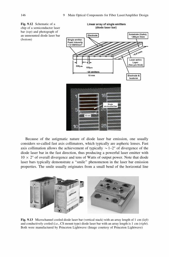
Because of the astigmatic nature of diode laser bar emission, one usuallyconsiders so-called fast axis collimators, which typically are aspheric lenses. Fastaxis collimation allows the achievement of typically *1–2� of divergence of thediode laser bar in the fast direction, thus producing a powerful laser emitter with10 9 2� of overall divergence and tens of Watts of output power. Note that diodelaser bars typically demonstrate a ‘‘smile’’ phenomenon in the laser bar emissionproperties. The smile usually originates from a small bend of the horizontal line

Fig. 9.12 Schematic of achip of a semiconductor laserbar (top) and photograph ofan unmounted diode laser bar(bottom)

Fig. 9.13 Microchannel cooled diode laser bar (vertical stack) with an array length of 1 cm (left)and conductively cooled (i.e., CS mount type) diode laser bar with an array length is 1 cm (right).Both were manufactured by Princeton Lightwave (Image courtesy of Princeton Lightwave)

146 9 Main Optical Components for Fiber Laser/Amplifier Design

where single emitters are located; it is a technological drawback that affects fastaxis collimation and focusing of the diode laser bar radiation. This in turn mayaffect diode laser fiber-coupling efficiency, which is critical for fiber laser and fiberamplifier applications.

9.1.3.3 Diode Laser Stack of Bars

Further power scaling of the diode lasers uses one- or two-dimensional stacks ofseveral diode bars. Usually, bars are arranged in horizontal or vertical directions,depending on applications. Most fiber laser applications require efficient fiber-coupled high-power diode laser beam delivery for optical pumping. Horizontallystacked diode laser bars are usually used in high-power diode pumping ofcrystalline or glass slab lasers. Vertical stacks can be manufactured from a two-dimensional wafer packaged into the heat sink. An example schematic of a water-cooled diode laser stack is shown in Fig. 9.14.

Packaging the diode laser bars close to each other provides many advantageswith respect to the output beam and beam management. However, heat removalusually applies restriction to the separation of the individual bars. Because of thisreason, most high-power diode laser stacks have low overall brightness, and onemay consider diode stack polarization or spectral beam combining technologies.Similar to the fast axis microlensing of diode laser bars, two-dimensional diodelaser stacks are microlensed by a mask (matrix) of high-aperture aspheric lenses.

Commercially available diode laser stacks may be arranged in two-dimensionalstructures (vertically and horizontally), providing more than several hundredsWatts of diode laser emission. A diode laser stack–beam combination allows theachievement of thousands of watts and is very important for power scaling of fiberlasers. The possibility of fiber-coupling options creates additional advantages for

Fig. 9.14 Schematic of ahigh-power, water-cooledvertical laser diode stack. Thelaser diode stack height istypically 10–50 mm but mayvary beyond this dimension,depending on several factorsincluding power level,operational duty factor,number of bars, and bar-to-bar distance. (Permission touse granted by NewportCorporation. All rightsreserved)

9.1 Laser Diodes 147

fiber laser technology because it gives an opportunity to build the all-fiber (no freespace) high-power fiber laser systems that are required for many industrial andmilitary applications.

9.1.4 Fiber-Coupled Diode Lasers

Although the fiber-coupled diode laser concept has existed for years, scientists andengineers started sensing a real advantage in using fiber pigtails of diode laserswith the development of fiber lasers and fiber amplifiers. The advantages of usinglight emerging from optical fiber compared with direct diode laser emissioninclude the following:

1. For many applications that use direct light from a laser diode, it is convenient touse a fiber-coupled diode laser beam to deliver the laser light to the place whereit is needed.

2. The fiber-coupled light has a circular geometry (unlike direct emissions fromedge-emitting diode lasers), which is very convenient for many subsequentbeam transformations.

3. The use of fiber-coupled laser diodes in laser pumping applications allows theachievement of easy (alignment-free) diode laser maintenance, including diodelaser replacement and service.

4. The manageable fiber length of fiber-coupled diode lasers allows the achieve-ment of separate locations for the pump and the main laser cavity. Such flex-ibility in the relative displacement of pump and cavity optics is especiallyimportant for high-power laser systems, in which the thermal management ofboth diode lasers and active laser media requires careful consideration.

5. In fiber lasers and amplifiers in which an all-fiber approach is applied, fiber-coupled diode lasers allow all-fiber solutions; together with other fiber-coupledcomponents, the entire system is practically alignment free.

Usually, diode lasers are fiber coupled into single-mode or multimode opticalfibers, depending on the mode structure of the original diode laser. Fiber couplingefficiencies depend strongly on the power level of the diode laser, the diode laserstructure, and the approach of fiber coupling (i.e., lens based or fiber profiling).Power diode laser systems with high average power may create overheatingconditions at the fiber entrance, which in turn may result in stress and damage ofthe fiber endface. Special care has to be taken with the fiber termination enclosurefacing the diode laser beam.

When fiber profiling is used, the fiber tip that faces the laser diode-emittingsurface is shaped by polishing for efficient, direct coupling of the diode laserradiation. Efficiencies of more than 92 % are achieved using such a fiber-couplinggeometry. This high fiber-coupling efficiency is very important for high-powerdiode lasers, where minimization of heat dissipation plays an important role in the

148 9 Main Optical Components for Fiber Laser/Amplifier Design

reliability of the component. However, the direct coupling of the fiber laser beaminto the fiber prevents the possibility of locating additional optical componentsbetween the diode laser and fiber, such as dichroic mirrors (for protection againstback reflection) or optical isolators (e.g., in DFB fiber-coupled diode lasers, whereoptical feedback compromises DFB diode laser parameters and therefore incor-poration of an optical isolator is a must).

Fiber-coupled diode lasers are characterized by power—spectral as well asoptical parameters of the fiber into which the diode laser light has been coupled.Usually, optical parameters of the fiber include the fiber core diameter and corenumerical aperture. The most common fiber diameters of fiber-coupled diodelasers are 6, 9, 50, 105, 200, 400, and 600 microns, whereas numerical aperturesusually are 0.12, 0.15, or 0.22.

Along with obvious and important advantages, a fiber-coupling approach hasseveral disadvantages, including the following:

• Higher cost compared with free-space diode emitters.• Decreased output power because fiber coupling has limited efficiency, especially

for high-power diode laser bars.• Inability (at times) to insert an additional optical component, such as an optical

isolator, between the diode laser output and fiber input.• For multimode diode lasers using multimode fibers, the polarization maintaining

propagation of the diode laser beam is lost.• Fiber-coupled diode lasers are more susceptible to optical damage due to back

reflections; they require special consideration for protection against opticaldamage using additional in-line beam splitters and filters.

9.2 Fiber-Coupled Polarization-Maintainedand Non-polarization-Maintained OpticalComponents

This section reviews the most common fiber-optic components used in fiber lasersand fiber amplifiers. Depending on the manufacturing process used in the devel-opment process, there are two main categories of fiber-optic components: free-space components and fused components. Free-space fiber-optic componentsemploy free-space optics, such as lenses and optical filters, in between input andoutput fiber ports of the device. In the case of fused components, all fiber ports arefused together to create optical contact. In either approach, however, the mainprinciple (i.e., the principle of optical brightness preservation) has to be main-tained in order to design reliable and low-loss systems. Unmatched opticalbrightness usually results in excess heat generated in the place of transition fromone aperture to another, which in turn impact power tolerance and power trans-mission efficiency/loss of the device. Fiber-coupled optical components that arenot brightness limited allow more than 95 % of power transmission.

9.1 Laser Diodes 149

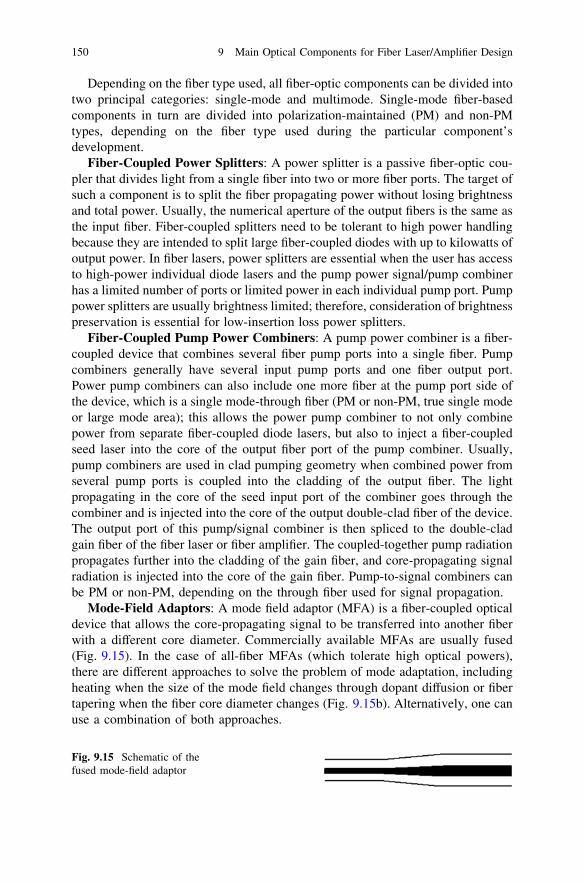
Depending on the fiber type used, all fiber-optic components can be divided intotwo principal categories: single-mode and multimode. Single-mode fiber-basedcomponents in turn are divided into polarization-maintained (PM) and non-PMtypes, depending on the fiber type used during the particular component’sdevelopment.

Fiber-Coupled Power Splitters: A power splitter is a passive fiber-optic cou-pler that divides light from a single fiber into two or more fiber ports. The target ofsuch a component is to split the fiber propagating power without losing brightnessand total power. Usually, the numerical aperture of the output fibers is the same asthe input fiber. Fiber-coupled splitters need to be tolerant to high power handlingbecause they are intended to split large fiber-coupled diodes with up to kilowatts ofoutput power. In fiber lasers, power splitters are essential when the user has accessto high-power individual diode lasers and the pump power signal/pump combinerhas a limited number of ports or limited power in each individual pump port. Pumppower splitters are usually brightness limited; therefore, consideration of brightnesspreservation is essential for low-insertion loss power splitters.

Fiber-Coupled Pump Power Combiners: A pump power combiner is a fiber-coupled device that combines several fiber pump ports into a single fiber. Pumpcombiners generally have several input pump ports and one fiber output port.Power pump combiners can also include one more fiber at the pump port side ofthe device, which is a single mode-through fiber (PM or non-PM, true single modeor large mode area); this allows the power pump combiner to not only combinepower from separate fiber-coupled diode lasers, but also to inject a fiber-coupledseed laser into the core of the output fiber port of the pump combiner. Usually,pump combiners are used in clad pumping geometry when combined power fromseveral pump ports is coupled into the cladding of the output fiber. The lightpropagating in the core of the seed input port of the combiner goes through thecombiner and is injected into the core of the output double-clad fiber of the device.The output port of this pump/signal combiner is then spliced to the double-cladgain fiber of the fiber laser or fiber amplifier. The coupled-together pump radiationpropagates further into the cladding of the gain fiber, and core-propagating signalradiation is injected into the core of the gain fiber. Pump-to-signal combiners canbe PM or non-PM, depending on the through fiber used for signal propagation.

Mode-Field Adaptors: A mode field adaptor (MFA) is a fiber-coupled opticaldevice that allows the core-propagating signal to be transferred into another fiberwith a different core diameter. Commercially available MFAs are usually fused(Fig. 9.15). In the case of all-fiber MFAs (which tolerate high optical powers),there are different approaches to solve the problem of mode adaptation, includingheating when the size of the mode field changes through dopant diffusion or fibertapering when the fiber core diameter changes (Fig. 9.15b). Alternatively, one canuse a combination of both approaches.

Fig. 9.15 Schematic of thefused mode-field adaptor

150 9 Main Optical Components for Fiber Laser/Amplifier Design

Because most applications deal with fundamental mode fiber lasers andamplifiers, the aim of an MFA is to preserve the energy (loss-free propagation) inthe fundamental mode of the fiber; therefore, this mode transformation has to bedone adiabatically. The adiabaticity criteria use an assumption that the charac-teristic angle of tapering should be smaller than the diffraction angle of the field ateach point along the taper [5]. The analytical expression for the diffraction anglefor step index fiber is as follows:

hD ¼2�

ffiffiffiffiffiffiffiffi

ln Vp

V� NA ð9:9Þ

where V is the V-number and NA is the fiber core numerical aperture. The dif-fraction angle applies for the fundamental mode of the fiber only. Another way toformulate the mode-matching criteria is to require that core sizes and numericalapertures of the input and output fibers (or their V-numbers) have to be matched.This condition creates challenges in the manufacturing process.

In general, MFAs are usually low-insertion-loss devices, unless backwardpropagation of the optical signal takes place when they become brightness limited.MFAs play an important role in the development of high-power fiber laser systemsand amplifiers, which often use multistage geometries with increased gain andfiber core diameters. MFAs can be made in a PM or non-PM configuration,depending on the fibers used in its input and output ports.

Cladding light strippers: Optical devices that strip residual cladding propa-gating light while preserving core propagating energy are called cladding lightstrippers (or cladding beam dumps). The ability to strip cladding light fromdouble-clad fiber is required for many different reasons during fiber laser design.Cladding propagating power can reach power levels of the hundreds of Watts (notethat cladding NA is typically several times higher than NA of the core). By locallychanging cladding NA (e.g., by changing the refractive index of the materialsurrounding cladding), it is possible to achieve significant attenuation of thecladding propagating light. Figure 9.16 demonstrates an example of the use of acladding power stripper in fiber laser [6].

Fig. 9.16 Example of a simple fiber laser/amplifier design employing a cladding power stripper[6]. (Image courtesy of SPIE)

9.2 Fiber-Coupled Polarization-Maintained 151

As shown in Fig. 9.15a, Wetter et al. [6] used an all-fiber 6 ? 191 TFB splicedto a 20–400 Yb3+-doped DCF gain fiber. The fiber laser resonator is formed by twofiber Bragg gratings (FBGs), which act as the laser cavity mirrors (i.e., highreflector and output coupler). A cladding light stripper is introduced after the gainfiber to strip all the unwanted light in the forward and backward direction. Theauthors [6] achieved attenuation of more than 20 dB in the cladding, practicallywithout signal loss. After stripping the damped cladding, light energy has to beproperly distributed along the stripper and heat sink. Cladding strippers canpotentially strip tens to hundreds of Watts in high-power fiber lasers and amplifiers.

Optical Isolators: A fiber-coupled optical isolator is an optical device thatallows for unidirectional core propagation of light with a high degree of opticalisolation in the backward propagation direction (Fig. 9.17). Fiber-coupled opticalisolators can be single or double/multistage depending on the degree of requiredoptical isolation of the core-propagating light.

9.2.1 Polarization-Dependent Optical Isolators

Figure 9.18 shows the structure of a polarization-dependent optical isolator. Theoptical isolator consists of a polarizer, an analyzer, and a 45� Faraday rotatorinserted between them. The polarizer and analyzer main axes are rotated at 45�relative to each other.

Fig. 9.17 Schematic viewof a packaged two-portfiber-coupled opticalisolator

Fig. 9.18 Composition ofpolarization-sensitive opticalisolator (Image courtesy ofFDK Corporation)

152 9 Main Optical Components for Fiber Laser/Amplifier Design

When light propagates forward through the optical isolator, it first goes throughthe polarizer, where it is transformed into a linearly polarized light. Then, the lightpasses through the Faraday rotator, where the polarization plane of the lightentering the rotator is rotated 45� to its original orientation. Finally, the lightpasses through the analyzer without loss because the analyzer is tilted in such away that its polarization plane is set in the same direction as the light exiting therotator. On the way back, the light first passes through the analyzer, where it istransformed into linearly polarized light. Then, it passes through the Faradayrotator, getting a 45� rotation of its polarization direction in the same rotationdirection as on the way forward in the initial tilt. Finally, because the total tilt ofthe back-propagating light polarization plane is 90�, it is completely blocked bythe polarizer.

It is important to mention the recent developed all-fiber isolators. These devicesare based on 56 wt % terbium (Tb)-doped silicate fiber, and the fiber polarizers aremade of Corning SP1060 single-polarization fiber [7]. Sun et al. [7] demonstrated17 dB optical isolation at 1,053 nm. This approach shows the potential forachieving compact, high-power isolators in the near future.

Polarization-dependent isolators have wide applications, not only betweenstages of multistate fiber amplifiers but also in semiconductor lasers, especially theDFB type, which are very sensitive to backward-propagating light. The opticalisolators are usually compared by their insertion loss and degree of isolation at thewavelength of interest.

9.2.2 Polarization-Independent Optical Isolators

Unlike polarization-dependent optical isolators, polarization-independent isolatorshave a 45� Faraday rotator placed between two wedge-shaped birefringent plates(Fig. 9.16a and b). Birefringent plates can be manufactured from TiO2 singlecrystals (rutile), which demonstrate superior extinction ratios and big differencesbetween ordinary and extraordinary beam refractive indexes.

When light enters a polarization-insensitive isolator, it first undergoes apolarization separation into ordinary and extraordinary beam components by thefirst birefringent plate (see Fig. 9.19a). The two beams then enter a Faradayrotator; the polarization planes are each rotated 45� after passing through therotator. After that, the ordinary and extraordinary beams pass through a secondwedged birefringent plate. The second birefringent plate has an optic axis orientedin such a way that the relationship between ordinary and extraordinary beams ismaintained. Finally, both beams are refracted in an identical parallel direction afterpassing through the second wedged birefringent plate.

Backward-propagating light incident on the same optical isolator is separatedinto ordinary and extraordinary beams, whose relationship is reversed with that ofa forward light due to the nonreciprocality of the Faraday rotation (see Fig. 9.19b).Eventually, when reaching first birefringent plate, the beams do not become

9.2 Fiber-Coupled Polarization-Maintained 153

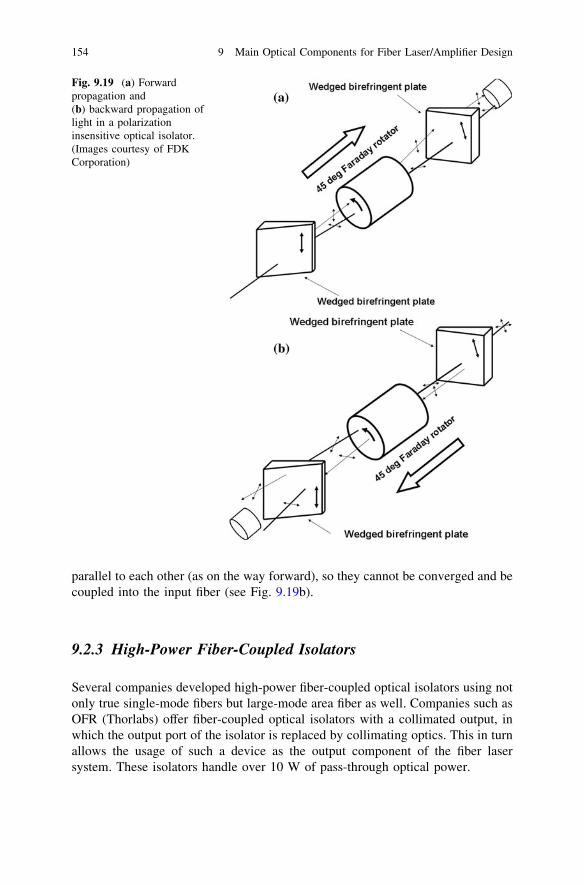
parallel to each other (as on the way forward), so they cannot be converged and becoupled into the input fiber (see Fig. 9.19b).

9.2.3 High-Power Fiber-Coupled Isolators

Several companies developed high-power fiber-coupled optical isolators using notonly true single-mode fibers but large-mode area fiber as well. Companies such asOFR (Thorlabs) offer fiber-coupled optical isolators with a collimated output, inwhich the output port of the isolator is replaced by collimating optics. This in turnallows the usage of such a device as the output component of the fiber lasersystem. These isolators handle over 10 W of pass-through optical power.

Fig. 9.19 (a) Forwardpropagation and(b) backward propagation oflight in a polarizationinsensitive optical isolator.(Images courtesy of FDKCorporation)

154 9 Main Optical Components for Fiber Laser/Amplifier Design

Optical Circulators: A fiber-coupled optical circulator is a passive N-portdevice that couples light from port 1 to port 2, port 2 to port 3, and so on, to portN - 1 to port N. It has a high degree of isolation in opposite directions. Opticalcirculators allow unidirectional propagation of the light traveling in the fiber coreand therefore are very useful in ring-fiber resonators.

Two principal structural components are shared by most optical circulators: apolarization rotation device (usually a Faraday rotator) and a polarization beam-splitting device (usually a polarizing prism or set of prisms). In the case of fiber-coupled circulators, each circulator port is effectively fiber coupled. The operationprinciple of an optical circulator is very similar to that used in an optical isolator.Using a polarization rotation of the light propagating forward through the system,an optical circulator uses the same polarization rotation again when the light is onthe way back. Unlike isolators in which the back-propagating beam gets dumped,an optical circulator uses backward-propagating light as an output signal of itsoutput ports (i.e., from port N to port N ? 1). However, there is approximately30 dB of isolation between port N and port N - 1. A typical view of the packagedfiber-coupled optical circulator is shown in Fig. 9.20.

The main challenge during the design of the optical circulator is to obtain asmall insertion loss. Lately, because of growing demand for optical circulatorsused in high-power fiber laser technology, scaling the power tolerance of opticalcirculators is an important task. The following sections provide the design struc-ture of some optical circulators as described in the literature.

9.2.4 Polarization-Dependent Circulator

Figure 9.21 shows a conventional polarization-sensitive (polarization-dependent)optical circulator [8]. Forward propagation is similar to that in optical isolator.Because the Faraday rotator rotates the propagating light polarization in the samedirection (e.g., clockwise), one can easily reproduce the path of the light beamthrough the circulator shown in Fig. 9.21. In the case of fiber-coupled circulators,each port is fiber coupled (not shown in the figure).

(Image courtesy of the Optical Society of America)

Fig. 9.20 The schematic andlight propagation directionsof a packaged three-portfiber-coupled opticalcirculator

9.2 Fiber-Coupled Polarization-Maintained 155

9.2.5 Polarization-Independent Circulator

The polarization-independent optical circulator is somewhat more complicatedbecause it must include polarization-insensitive components or set of polarization-sensitive components that produce overall device polarization insensitivity. Fig-ure 9.22 shows an example design of the polarization-insensitive circulator, whichuses prism-based polarization separators, a Faraday rotator, and a half-wave plate.Shirasaki et al. [9] used total internal reflection to make ordinary and extraordinarybeams adjacent (Fig. 9.23).

The Faraday rotator employs a permanent magnet and Faraday garnet crystal.High-power, compactly packaged fiber-coupled optical circulators still demon-strate challenges. However, some companies (e.g., OFR) have already startedcommercial development of such circulators.

Fiber Bragg Gratings: The FBG is an optical device that employs a constantperiod grating (uniform grating) of higher and lower refractive indices in the fibercore (or in the vicinity of the ring surrounding the core) along the light-propa-gating direction (Fig. 9.24). This technology uses a photosensitive optical fiberthat is exposed to deep ultraviolet laser light through a grating, thus creating aninterferometric pattern along the light propagation direction in the fiber core and amodulated profile of the fiber core refractive index.

Depending on the refractive index grating period and grating length, FBGsoperate as optical filters or mirrors. FBGs play an important role in spectral line-width control of fiber lasers. The reflectivity of the uniform grating with constantmodulation amplitude and constant period can be obtained using the coupled modetheory [10], given by the following formula:

Fig. 9.21 Schematic viewof a polarization-dependentfour-port optical circulator [8]

Fig. 9.22 Prism-basedpolarization separator [9].(Image courtesy of theOptical Society of America)

156 9 Main Optical Components for Fiber Laser/Amplifier Design

RðL; kÞ ¼ j2 sin h2ðs � LÞDb2 sin h2ðs � LÞ þ s2 cos h2ðs � LÞ

ð9:10Þ

where j ¼ pDnk Mpower is the power coupling coefficient for the sinusoidal variation

of the refractive index, Db ¼ b� p=K is the detuning wavevector, b ¼ 2pn0k is the

propagation constant, and Mpower is the fraction of the fiber mode power contained

in the fiber core and s ¼ffiffiffiffiffiffiffiffiffiffiffiffiffiffiffiffiffiffiffi

j2 � Db2p

.The FWHM of the spectral bandwidth for the uniform diffraction grating is as

follows [11]:

Dk ¼ kBR

ffiffiffiffiffiffiffiffiffiffiffiffiffiffiffiffiffiffiffiffiffiffiffiffiffiffiffiffiffiffiffiffi

Dn

2n0

� �2

þ 1N

� �2s

ð9:11Þ

where R is the coefficient that determines the grating strength (R = 1 for stronggrating and R = 0.5 for weak grating), Dn is the refractive index modulation, kB isthe central wavelength of operation (Bragg wavelength), and N is the number ofgrating lines along the whole length of the grating.

9.2.6 Chirped FBG as a Self-Phase ModulationCompensator

In a pulsed fiber laser system as a result of self-phase modulation (SPM; discussedin detail in Chap. 10), the original laser pulse is chirped. Using a special FBG typecalled chirped FBG (CFBG), one can compensate for the pulse chirp and ensureundisturbed laser pulse propagation in the amplifier. CFBG is an FBG where the

Fig. 9.23 Schematic of apolarization-insensitiveoptical circulator [9]. (Imagecourtesy of the OpticalSociety of America)

9.2 Fiber-Coupled Polarization-Maintained 157

regions with high refractive index are not uniformly spaced or are not perpen-dicular to the length of the fiber (Fig. 9.25).

If we introduce a chirp bandwidth Dkchirp and an effective index of refractionneff and FBG period K, one can express wavelength chirp bandwidth of thegratings as:

Dkchirp ¼ 2neffDKchirp ð9:12Þ

where DKchirp = Klong - Kshort. FBG dispersion is then described by the fol-lowing expression:

AD ¼ 2Lgrating � 1�DkchirpVgroup

� � ð9:13Þ

where Lgrating is the FBG length and Vgroup is the group velocity. A typical value ofthe FBG is 10 ns/m/Dkchirp.

Depending on the sign of the FBG dispersion, AD, one can either compress orbroaden the optical pulse. For Gaussian-shaped laser pulses, the followingexpression is used to calculate the pulse width deviation from its original value:

tp ¼ tpð0Þ 1þ 2pc DkchirpADLgrating

� �

=k2� 0:5 ð9:14Þ

where tp(0) is the original pulse width of the laser entering the amplifier. Bybalancing the grating length, grating dispersion, and chirp bandwidth, one cancontrol the pulse width of the pulse propagating in the amplifier.

Fig. 9.24 Schematic view ofthe fiber Bragg grating

Fig. 9.25 Schematicexample of a chirped fiberBragg grating

158 9 Main Optical Components for Fiber Laser/Amplifier Design

9.2.7 A Few Words About Fiber Endface Preparation

In addition to fiber cleaving, there are four common types of fiber end preparationsused in fiber lasers, either for fiber-coupled pump diode terminations or in outputports of fiber laser systems (Fig. 9.26):

1. A flat polish of the end face of the fiber, which results in back reflection ofabout -14 dB (i.e., 4 %).

2. A physical contact polish produces a slightly curved end face that forces thefibers in the mating connectors into contact. This reduces back reflection toabout -40 dB by eliminating the fiber-to-air interface. This is the most com-monly used preparation.

3. An angled physical contact polish adds 8 degrees or more to a flat polishcondition. When used with fiber-to-fiber contact, this type of polishing keepsthe fiber ends together. Also, light at the interface is reflected at a large angle,missing the core. Back reflections can be reduced to about -70 dB with thistechnique, or even more if larger angles are used.

4. A high-power flat-polished end face preparation is typically used for high-power fiber-coupled diode laser termination. The idea is to spatially separatethe metallic part of the ferrule from the bare fiber end to prevent the depositionof metal particles on the fiber end face (e.g., in case back-propagating intenselaser light hits the area next to the fiber).

Fiber end face preparation (in terms of surface profile) plays an important rolein high-power fiber lasers because it determines optical back reflection into thegain material, which in turn may reduce fiber laser performance. Note that a highdegree of cleanliness of the termination surface is required in most high-powerfiber laser applications due to a high probability of damage to a poorly cleanedsurface.

Fig. 9.26 The mostcommonly used fiber end facepreparation types (applied toferrule-based connectors)

9.2 Fiber-Coupled Polarization-Maintained 159

References

1. N.G. Basov, B.M. Vul, YuM Popov, Quantum-mechanical semiconductor generators andamplifiers of electromagnetic oscillations. Sov. Phys. JETP 10, 416–417 (1959)

2. R.N. Hall, G.E. Fenner, J.D. Kingsley, T.J. Soltys, R.O. Carlson, Coherent light emissionfrom GaAs junctions. Phys. Rev. Lett. 9(9), 366–369 (1962)

3. S.D. Offsey, J.M. Woodall, A.C. Warren, P.D. Kirchner, T.I. Chappell, G.D. Pettit, Appl.Phys. Lett. vol. 48, 475 (1986)

4. S.M. Sze, Physics of semiconductor devices (Wiley-Interscience, New York, 1981), pp. 8805. J.D. Love, Spot size, adiabaticity and diffraction in tapered fibers. Electron. Lett. 23, 993–994

(1987)6. A.Wetter, M.Faucher, B.Sévigny, High power cladding light strippers, in Proceedings of

SPIE, vol. 6873, 687327.1–8, (2008)7. L. Sun, S. Jiang, J.D. Zuegel, J.R. Marciante, All-fiber optical isolator based on Faraday

rotation in highly terbium-doped fiber. Opt. Lett. 35, 706–708 (2010)8. T. Matsumoto, K. Sato, Polarization-independent optical circulator: an experiment. Appl.

Opt. 19, 108–112 (1980)9. M. Shirasaki, H. Kuwahara, T.Obokata, Compact polarization-independent optical circulator.

Appl.Opt. 20, 2683– 2687 (1981)10. D.K.W. Lam, B.K. Garside, Characterization of single-mode optical fiber filters. Appl. Opt.

20, 440–445 (1981)11. P.S. Russell, J.L. Archambault, L. Reekie, Fiber gratings. Physics World, October 1993 issue,

pp. 41–46 (1993)12. I. Gorog, P.V. Goedertier, J.D. Knox, I.Ladany, J.P. Wittke, A.H. Firester, Information

scanning technology: applications of CW AlGaAs injection lasers. Appl. Opt. 15, 1425–(1976)

13. M.I. Nathan, Semiconductor lasers. Appl. Opt. 5, 1514–1528 (1966)

160 9 Main Optical Components for Fiber Laser/Amplifier Design

Chapter 10High-Power Fiber Lasers

High-power fiber lasers occupy probably the most challenging and demandingplace in the whole field of fiber laser technology; they also are state of the art. Bothcontinuous-wave (CW) and pulsed high-power fiber laser systems constantlyrequire technological advances. This chapter describes the main challenges in thedevelopment of high-power fiber lasers—the solution of which creates a path tosuccessful laser development.

The main challenges in scaling-up fiber laser power are:

1. Nonlinear effects must be eliminated. For CW fiber lasers, two main nonlineareffects restrict power scaling: stimulated Brillouin scattering (SBS) and stim-ulated Raman scattering (SRS). Large core size and short fiber length willincrease SRS and SBS thresholds.

2. For close to diffraction-limited beam quality (i.e., fundamental LP01 modeoperation) at high operation powers, large-mode area (LMA), double-clad (DC)fiber with a high doping level of the active ion is required.

3. Core glass and end-facet damage must be eliminated because they may lead tofiber laser efficiency degradation or fatal breakdown.

4. High-power and high-brightness diode laser pumps and pump-coupling systemswith high damage thresholds and high pump/signal power coupling efficiencywith low thermal load must be developed.

5. Thermal management must occur to avoid heat-induced damage. Thermaleffects may cause instability or even reduction in beam quality, change in laserwavelength or line-width, or polarization instability. In the case of challengesrelated to preservation of good beam quality, LMA fiber should be used with anumerical aperture (NA) below a certain value to discriminate high-ordermodes using coiling technology. The temperature dependence of the refractiveindex has a direct influence on the NA and hence the mode-discriminationcapabilities of the LMA fiber.

6. Photodarkening must be addressed.7. Robust, commercially available fiber-optic components and system configura-

tions must be developed, such that the whole laser system maintains its

V. Ter-Mikirtychev, Fundamentals of Fiber Lasers and Fiber Amplifiers,Springer Series in Optical Sciences 181, DOI: 10.1007/978-3-319-02338-0_10,� Springer International Publishing Switzerland 2014

161

efficiency, beam quality, and damage-free operation while operating at highaverage power.

8. Polarization maintenance problems must be addressed to maintain precisephase control for coherent beam combining and nonlinear frequencyconversion.

Processes in high-power CW fiber lasers that lead to bulk and surface damageof the fiber material include the following:

• Optical nonlinearities create self-pulsing in high-power fiber lasers. Self-pulsingis thought to be a reason for self-mode locking and self-Q-switching in opticalfibers and causes self-focusing, resulting in bulk optical damage of the fiberglass.

• Thermal stress on the output of the fiber produces surface damage. A powerlevel of 200–500 kW/cm2 (depending on the condition of the fiber end surface)is considered to be the upper limit for damage-free fiber laser operation due tothermal stress.

Prevention strategyThe threshold of SBS and SRS optical processes can be increased by the

following:

1. Increasing laser line-width when possible.2. Decreasing gain fiber length.3. Increasing gain fiber core diameter.4. End-capping the fiber.5. Reducing thermal load.

In most cases, during development of high-power fiber lasers, the followingnonlinear processes have to be taken into consideration: SRS, SBS, four-wavemixing (FWM), self-phase modulation (SPM), cross-phase modulation (XPM),and self-focusing. These nonlinear processes play a key role in the development ofreliable fiber laser systems and will be discussed later in this chapter.

Some authors have suggested using new fiber materials, such as YAG, toreplace silica to ease several challenges of fiber lasers’ power scaling. By replacingsilica with YAG in the fiber core and optimizing fiber parameters, such as corediameter and fiber length, Parthasarathy et al. [1] showed that the limit for theYAG fiber laser is 6 kW per fiber in a multimode operation (compared to 1.8 kWfor a silica-based fiber laser). Because of the smaller SBS gain in YAG(\10–12 m/W), the maximum output power of 30 kW can be achieved from asingle fiber without a significant increase in fiber core diameter [1]. Significantimprovement is also expected for single-mode laser operation using this approach.

162 10 High-Power Fiber Lasers

10.1 Gain Fiber Pumping Technology for High-PowerFiber Lasers

The way that pumping radiation is coupled into the gain fiber determines the fiberlaser pumping scheme. There are two main types of such coupling: when pumpinglight is coupled directly into the core (so-called core-pumped gain fibers) and whenpumping light is coupled into the cladding (so-called clad-pumped gain fibers).Each pumping scheme has its advantages and disadvantages. Depending on theapplication, researchers and engineers give preference to one of these pumpcoupling schemes. This section compares the two fundamental pumping schemes,which should help the reader to understand the pump-type selection strategy.

Core Pumping: This pumping scheme is applied to single-clad gain fibers(Fig. 10.1). Its main advantages include a high core absorption, which allows for ashort gain fiber length. However, it is restricted by its limited pump power due tohigh-brightness (single transverse mode) diode lasers, which are required forsuccessful core pumping. This results in core darkening with creation of parasiticabsorption due to high power density.

Clad Pumping: This pumping scheme is applied to DC and triple-clad (TC) gainfibers. A low-index polymer is typically used as a second/third (outer) cladding(Fig. 10.2). Its main advantages include the ability to couple high-power pumpradiation from low-brightness diode lasers while maintaining the fundamentalmode of the fiber laser radiation emerging from the doped fiber core. The downsideis reduced effective pump absorption; therefore, longer fibers are required foreffective absorption of the pump, which in turn affects the power threshold ofnonlinear processes inside the core. Another limitation is reduced power densitydue to large clad diameters. For example, high-power densities are required for truethree-energy-level lasers, such as Er3+, and may be a limitation when reabsorptionsaturation is required. Nevertheless, using a DC fiber helps to scale fiber sources tohigher power levels, which are not achievable with core-pump geometry, as well ashigher pulse energies, because the large multimode inner cladding facilitates theuse of higher-power and lower-cost multimode pump sources.

Fig. 10.1 Typical structureof the single-clad Panda-typefiber (Image courtesy ofNufern)

10.1 Gain Fiber Pumping Technology for High-Power Fiber Lasers 163

10.2 Double-Clad Fibers and Clad-Pumping Technology

A DC fiber is an optical fiber with two claddings that are equally important forlight propagation through it. The main difference between single-clad fiber and DCfiber is the value of the refractive index of the outer cladding. This differenceallows the wave-guided propagation of light inside the cladding of DC fiber at thesame time that another wavelength of light is propagated in the DC fiber core. Atthe same time, cladding of the single-clad fiber has a purpose of creating wave-guiding condition for the core propagating light. Cladding of the single-clad fiberis not designed to be a waveguide. Usually in both cases of single- and DC fibers,the outer cladding is made of a polymer, which has a special lower refractive indexin the case of DC fibers.

Because the DC fiber can waveguide laser radiation in the cladding and coresimultaneously, DC fibers are widely used in fiber lasers and fiber amplifiers,especially with elevated power. Because of the bigger diameter of the claddingcompared to that of the core, it is much easier to launch higher pump power intothe cladding. In the case of DC fiber, the core is doped and acts as the gain mediumof the fiber amplifier or laser. The pump light is coupled into the inner cladding.While propagating along the fiber, the pump light rays cross the core area; in thisway, they perform optical pumping of the core, creating population inversion. Theeffective absorption coefficient of the light propagating along the cladding at thewavelength of the absorption for the ions in the doped core is reduced by a factorof the ratio of cladding-to-core areas.

The so-called clad-pumping technology was developed in the mid-1980s,basically revolutionizing the power scaling of fiber lasers and amplifiers with closeto diffraction-limited beam quality. There is only one main disadvantage in thedesign of practical fiber laser systems: a reduced (by a factor of cladding-to-corearea ratio) x ¼ Sclad=Score effective absorption coefficient, which in turn requires anincreased length of gain fiber to achieve full pump absorption. In addition to theincreased cost of the longer gain fiber, this disadvantage also reduces the threshold

Low index polymer

Fig. 10.2 Typical structureof the double-clad Panda-typefiber (Image courtesy ofNufern)

164 10 High-Power Fiber Lasers

of nonlinear processes inside the core. Therefore, for high peak power applica-tions, one may preserve short, single-clad, highly doped fiber. Note that the usageof a modified shape of the first cladding geometry (as opposed to round) was usedto aid absorption of pump light by the doped fiber core. OFS (Furukawa, Avon,CT) introduced the so-called star cladding geometry to optimize cladding pumpabsorption.

For a typical true single-mode DC fiber with 5 and 125-lm core and claddiameters, respectively, effective absorption of the core at the pump wavelength isreduced by a factor of (125/5)2 = 625. For example, in Yb3+-doped DC 5/125fiber developed by Nufern, this effective absorption coefficient reduction leads toabout 10 m of gain fiber required to absorb 99 % of pump power propagating incladding. However, the ability to launch several tens of watts into the DC 125micron cladding makes this type of fiber very popular and widely used.

10.2.1 Clad-Pumping Schemes

Several pumping schemes to launch pump light into DC fiber have been devel-oped. These schemes include end pumping, which launches pump light into one orboth opposite ends of the fiber; fused fiber bundling, in which several multimodefibers are fusion-spliced to the inner cladding; and V-groove side pumping, inwhich the pump beam is launched by total internal reflection from a V-shapedgroove cut into the inner cladding of the fiber. The main challenges of thesepumping schemes include obstruction of the fiber ends and limited scalability forend pumping; the need for DC fiber and a fused bundle with matching dimensionsfor the fused fiber combiner; and relatively high alignment sensitivity for V-grooveside pumping geometry.

On the other hand, wavelength division multiplexing (WDM) is a technique inwhich optical signals with different wavelengths transmitted together are separatedor combined while being transmitted separately. This technique was mostly usedfor optical fiber communications because of the power restrictions of these devices.However, they are more and more often used in fiber laser technology. Because ofthe free space optics that are a core technology of the free space, micro-optics basedWDM, until recently this method was mostly used for core-pumping geometry.With the development of TC fibers, which can tolerate high incident pump powers,WDM devices are also being used in clad-pumping configurations.

Among all mentioned DC fiber pump-coupling techniques, probably the mostwidely used in medium- to high-power fiber lasers and amplifiers is fused-fiberbundling, which can be manufactured with or without a signal fiber incorporatedinto the bundle of several multimode fibers. Sometimes, the signal fiber (which canbe an LMA or single-mode fiber) is called a through fiber or signal-though fiber.Typical pump power transmission from pump fiber ports to the DC fiber claddingis more than 90 %, whereas signal fiber power transmission through a fibercombiner is more than 80 %.

10.2 Double-Clad Fibers and Clad-Pumping Technology 165

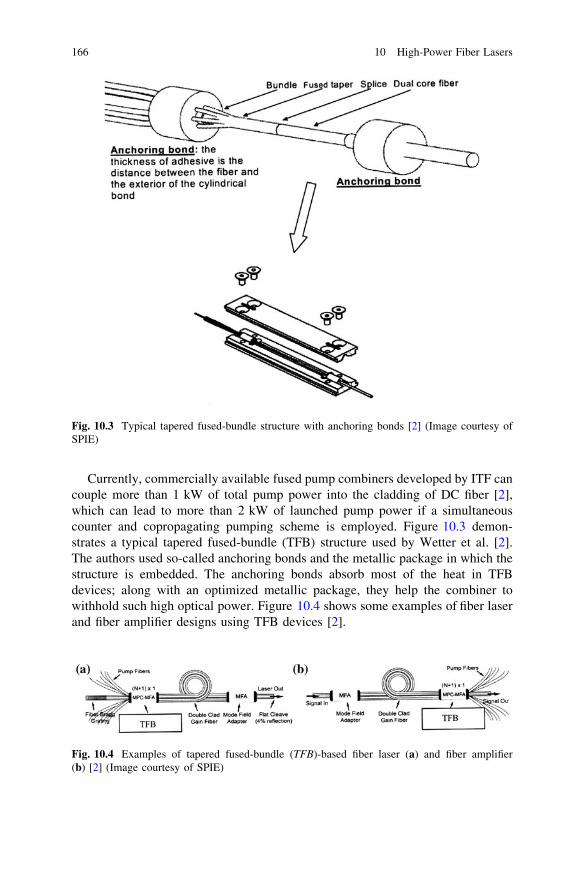
Currently, commercially available fused pump combiners developed by ITF cancouple more than 1 kW of total pump power into the cladding of DC fiber [2],which can lead to more than 2 kW of launched pump power if a simultaneouscounter and copropagating pumping scheme is employed. Figure 10.3 demon-strates a typical tapered fused-bundle (TFB) structure used by Wetter et al. [2].The authors used so-called anchoring bonds and the metallic package in which thestructure is embedded. The anchoring bonds absorb most of the heat in TFBdevices; along with an optimized metallic package, they help the combiner towithhold such high optical power. Figure 10.4 shows some examples of fiber laserand fiber amplifier designs using TFB devices [2].

Fig. 10.3 Typical tapered fused-bundle structure with anchoring bonds [2] (Image courtesy ofSPIE)

Fig. 10.4 Examples of tapered fused-bundle (TFB)-based fiber laser (a) and fiber amplifier(b) [2] (Image courtesy of SPIE)

166 10 High-Power Fiber Lasers

10.2.2 Clad-Pumping and Triple-Clad Fibers

TC fibers are all-glass DC fiber configurations in which the core, inner cladding,and outer cladding are all made of optical glass (Fig. 10.5). Similar to ordinary DCfibers, a polymer is used as a protection for the outer glass layer. The pumpinglight propagates inside the inner cladding, whereas the glass outer cladding servesas a reliable and rugged outer guiding layer with a low refractive index. This is astate-of-the-art gain fiber technology for high-power DC fibers.

Using TC fibers in fiber laser design and development has the followingadvantages:

1. Reliable pump guiding.2. No need for index matching during fiber recoating.3. High power tolerance for end-face pump coupling in fiber-optic devices, such

as WDM.

TC fiber is also a good solution for some clad-pumping applications in whichpumping light experiences optical absorption in the polymer cladding at the pumpwavelength, such as when induced by water absorption bands.

10.2.3 Free Space

Free-space pumping technology was historically first used in fiber lasers. Today, itis still a good option, especially for applications such as high-power fiber lasers, inwhich some of the fiber-coupled components are not readily available. Free-spacepump coupling can work well for both core- and clad-pumping applications.

With the appearance of DC fibers and clad-pumping technology, free-spacepump beam coupling regained popularity because of more relaxed requirementsfor focusing conditions. Among issues and challenges that have to be addressed inthe use of free-space pumping are fiber and lens holders, heat dissipating mounts,and other heat management problems. With a continuing reduction in prices forlens optics, such as aspheric lenses, the free-space pumping approach still attracts

Fig. 10.5 Typical structure of the triple-clad Panda-type fiber (Image courtesy of Nufern)

10.2 Double-Clad Fibers and Clad-Pumping Technology 167

the attention of researchers. However, for many applications, such as militaryapplications or those with harsh operational conditions, an alignment-freeapproach (i.e., all-fiber solution) looks more attractive, although at a higher costfor the all-fiber components and splicing equipment.

Today’s filter-based, fiber-coupled WDM components are free-space pump-coupling components packaged in a very compact enclosure with fiber pigtails ateach connection port (also with fused WDM fiber components). Several free-spacesolutions have been suggested in recent years, in addition to straightforward endfree-space pump coupling—namely, the embedded V-groove, prism coupler, andembedded mirror. Figure 10.6 summarizes these techniques. Most of the suggested

PUMP

Cladding

Cladding

Core

Reflector

Cladding

Cladding

Core

PUMP

PUMP

Prism

Prism

(a)

(b)

(c)

Fig. 10.6 a Diagram of anembedded mirrorside-pumping technique(cross-sectional side view).b Fiber V-grooveconfiguration [4] (Imagecourtesy of IET IEE).c Prism-based pump-couplerconfiguration for double-cladfibers

168 10 High-Power Fiber Lasers

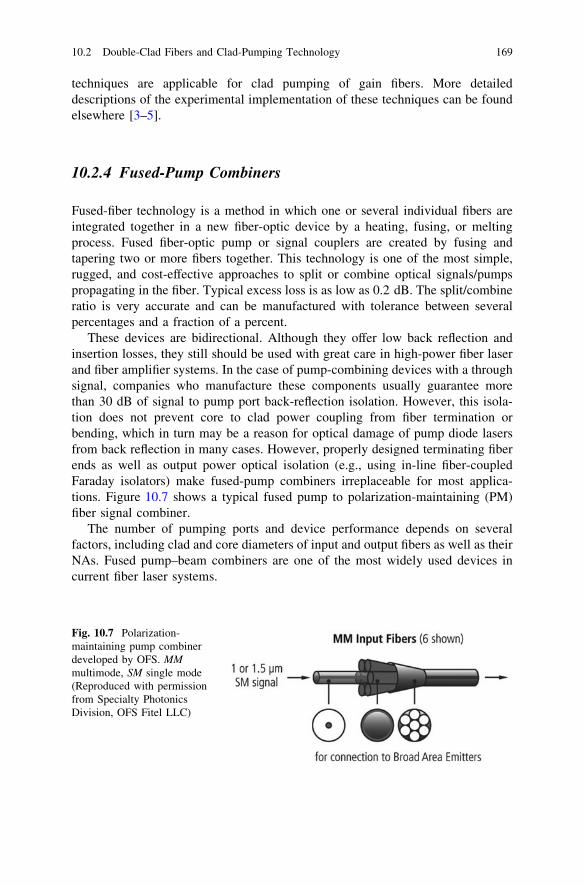
techniques are applicable for clad pumping of gain fibers. More detaileddescriptions of the experimental implementation of these techniques can be foundelsewhere [3–5].

10.2.4 Fused-Pump Combiners

Fused-fiber technology is a method in which one or several individual fibers areintegrated together in a new fiber-optic device by a heating, fusing, or meltingprocess. Fused fiber-optic pump or signal couplers are created by fusing andtapering two or more fibers together. This technology is one of the most simple,rugged, and cost-effective approaches to split or combine optical signals/pumpspropagating in the fiber. Typical excess loss is as low as 0.2 dB. The split/combineratio is very accurate and can be manufactured with tolerance between severalpercentages and a fraction of a percent.

These devices are bidirectional. Although they offer low back reflection andinsertion losses, they still should be used with great care in high-power fiber laserand fiber amplifier systems. In the case of pump-combining devices with a throughsignal, companies who manufacture these components usually guarantee morethan 30 dB of signal to pump port back-reflection isolation. However, this isola-tion does not prevent core to clad power coupling from fiber termination orbending, which in turn may be a reason for optical damage of pump diode lasersfrom back reflection in many cases. However, properly designed terminating fiberends as well as output power optical isolation (e.g., using in-line fiber-coupledFaraday isolators) make fused-pump combiners irreplaceable for most applica-tions. Figure 10.7 shows a typical fused pump to polarization-maintaining (PM)fiber signal combiner.

The number of pumping ports and device performance depends on severalfactors, including clad and core diameters of input and output fibers as well as theirNAs. Fused pump–beam combiners are one of the most widely used devices incurrent fiber laser systems.

Fig. 10.7 Polarization-maintaining pump combinerdeveloped by OFS. MMmultimode, SM single mode(Reproduced with permissionfrom Specialty PhotonicsDivision, OFS Fitel LLC)

10.2 Double-Clad Fibers and Clad-Pumping Technology 169

10.3 Large-Mode Area Fibers for High-Power,Diffraction-Limited Operation

An LMA fiber can be defined as an optical fiber that has a larger than true single-mode fiber core diameter, supporting only one or a few propagating spatial modes.The concept of LMA fibers was developed in the 1990s and mainly was inspired byresearchers who worked in the field of high peak power and single-frequency fiberlasers and amplifiers. For these applications, it is desirable to use optical fibers withincreased core areas, but preserving their single spatial-mode propagation as inmany cases. LMA fibers have a much higher threshold of practically all nonlin-earities due to the reduced intensities of the light propagating in the core, as well asa higher optical damage threshold. These features of LMA fibers make them irre-placeable for several applications, such as amplification of high peak power pulsesor for amplification or oscillation of single-frequency laser radiation in gain fibers.

It may seem that the easiest way to design such an LMA fiber is to create asmall difference between the core and cladding refractive indexes, which in turndecreases the NA of the core. However, because of the weaker guidance of thelight waves inside the core in this case, the propagating losses can become highfrom small imperfections of the inner fiber or from fiber bending. Therefore, suchan approach is very limited. Among existing reliable and bend loss-insensitiveLMA fibers (both doped and undoped) with close to one propagating spatial mode,the biggest core diameter is 10–15 lm with a NA of 0.06–0.08. Figure 10.8 showsthe typical panda-type PM LMA fiber profile, pictured from the fiber end.

To make LMA fibers more practical, several other techniques have been sug-gested. One of them is to achieve specially optimized refractive index profiles,which suppresses high-order mode propagation. This approach currently allowsthe achievement of up to a 30-lm LMA fiber core diameter. Note that fibermanufacturing with a sophisticated refractive index profile is a common challenge.

Fig. 10.8 Typicalpolarization-maintaininglarge-area mode 20/125double-clad fiber profile. Thismagnified photograph istaken from the fiber end(Image courtesy of nLight/Liekki)

170 10 High-Power Fiber Lasers

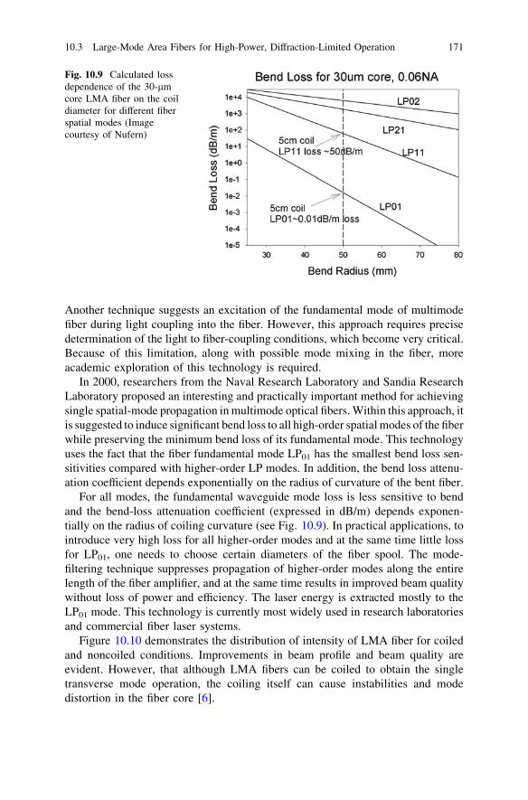
Another technique suggests an excitation of the fundamental mode of multimodefiber during light coupling into the fiber. However, this approach requires precisedetermination of the light to fiber-coupling conditions, which become very critical.Because of this limitation, along with possible mode mixing in the fiber, moreacademic exploration of this technology is required.

In 2000, researchers from the Naval Research Laboratory and Sandia ResearchLaboratory proposed an interesting and practically important method for achievingsingle spatial-mode propagation in multimode optical fibers. Within this approach, itis suggested to induce significant bend loss to all high-order spatial modes of the fiberwhile preserving the minimum bend loss of its fundamental mode. This technologyuses the fact that the fiber fundamental mode LP01 has the smallest bend loss sen-sitivities compared with higher-order LP modes. In addition, the bend loss attenu-ation coefficient depends exponentially on the radius of curvature of the bent fiber.

For all modes, the fundamental waveguide mode loss is less sensitive to bendand the bend-loss attenuation coefficient (expressed in dB/m) depends exponen-tially on the radius of coiling curvature (see Fig. 10.9). In practical applications, tointroduce very high loss for all higher-order modes and at the same time little lossfor LP01, one needs to choose certain diameters of the fiber spool. The mode-filtering technique suppresses propagation of higher-order modes along the entirelength of the fiber amplifier, and at the same time results in improved beam qualitywithout loss of power and efficiency. The laser energy is extracted mostly to theLP01 mode. This technology is currently most widely used in research laboratoriesand commercial fiber laser systems.

Figure 10.10 demonstrates the distribution of intensity of LMA fiber for coiledand noncoiled conditions. Improvements in beam profile and beam quality areevident. However, that although LMA fibers can be coiled to obtain the singletransverse mode operation, the coiling itself can cause instabilities and modedistortion in the fiber core [6].

Fig. 10.9 Calculated lossdependence of the 30-lmcore LMA fiber on the coildiameter for different fiberspatial modes (Imagecourtesy of Nufern)

10.3 Large-Mode Area Fibers for High-Power, Diffraction-Limited Operation 171

10.4 Nonlinear Processes in Optical Fibers and Their Rolein Fiber Laser and Fiber Amplifiers TechnologyDevelopment

All nonlinear processes that take place in optical fibers can be grouped into twomain categories: nonlinear scattering processes and nonlinear power dependenceof the fiber refractive index. Nonlinear processes that belong to first group includeSBS and SRS. The second group combines the processes of SPM, XPM, andFWM. From a practical viewpoint, SBS, SRS, and FWM mostly affect powerdistribution among several spectral lines corresponding to individual propagatingwaves, whereas SPM and XPM mostly affect spectral parameters of the propa-gating signals. Because of the crucial importance of nonlinear processes in fiberlasers design and development, each individual nonlinear process is described inmore detail below.

To review the main nonlinear processes that take place in fibers and play animportant role in the design and development of high-power fiber laser and fiberamplifier systems, several important parameters of optical fibers are introducedhere. First, consider the so-called effective length (Leff), which is determined by theabsorption characteristics of the fiber:

Leff ¼ 1P0

Z

PðzÞdz ¼Z

expð�lzÞdz ¼ 1� expð�lLÞl

ð10:1Þ

where P0 is the original optical power entering fiber, P(z) is the optical powerinside the fiber at given point z along the fiber length, L is the total fiber length, andl is the fiber absorption coefficient at the wavelength of light propagation.

Another important fiber parameter is the effective area Aeff, which is defined as:

Aeff ¼

R10 EaðrÞj j2r dr

ffi �2

R10 EaðrÞj j4r dr

ð10:2Þ

where Ea is the amplitude of the fundamental fiber mode and EaðrÞj j2¼ IðrÞ is theintensity of the fiber fundamental mode at radius r from the axis of the fiber.

Fig. 10.10 Near–field spatialprofile of the output from amultimode fiber amplifier(dcore = 25 lm) when thefiber is coiled (right) and notcoiled (left) [46] (Imagecourtesy of SPIE)

172 10 High-Power Fiber Lasers

In the case of conventional step index fibers, the field distribution of thefundamental mode is very well approximated by a Gaussian function. Therefore,the effective area of the fiber core is equal to:

Aeff ¼ pwðkÞ2 ð10:3Þ

where 2w(k) is the so-called mode field diameter (MFD) of the fiber core at wave-length k. Note that for fibers other than step index fibers (i.e., dispersion-shifted ordispersion-flattened fibers), the MFD cannot be approximated by a Gaussian functionand one should use other methods to determine MFD. But in the first approximationestimate of the effective core area of the fiber, in most practical cases of high-powerfiber lasers, MFD gives a good value that can be taken to determine Aeff.

Also, recall the power dependence of the glass refractive index, which plays animportant role in understanding the optical nonlinearities in fibers. As is wellknown, the glass refractive index can be expressed as:

n ¼ n0 þ n2P

Aeff

ð10:4Þ

where n0 is the linear refractive index of the fiber core (measured at low opticalpower levels), n2 is the nonlinear refractive index coefficient (which has a value of2.35 9 10-20 m2/W for silica), and P is the optical power of the propagating lightwave in watts.

10.4.1 Threshold Power of the Stimulated Scattering Process

It is useful here to review the basic formulas that determine the threshold of thestimulated scattering process. For the general case of a stimulated scatteringprocess (SRS or SBS) with an arbitrary pulse width of excitation (CW; i.e., sta-tionery or pulsed), one can derive an analytical expression for the scatteringprocess power threshold in a nonstationary regime of excitation. FollowingYa et al. [7], one can obtain:

gPthpeak

Aeff

Leff ¼ M when Ctp � 15 ð10:5Þ

and

gPthpeak

Aeff

Leff ¼M2 þ Ctp� �2

2Ctp

when Ctp � 15 ð10:6Þ

where g is a stimulated scattering gain given in cm/W, Pth peak is the threshold peakpower of the scattering process given in watts, Leff is the effective length of the fibergiven in centimeters, Aeff is the effective area of the fiber core given in cm2, U is thespectral line-width of spontaneous scattering process given in hertz, tp is thepropagating optical pulse width given in seconds, and M is a numerical factor that

10.4 Nonlinear Processes in Optical Fibers 173

determines a gain value of exp(M), which is usually considered as sufficient toamplify noise photons that shifted during stimulated scattering process opticalfrequency to the detectable level. The value of M is typically 30 for the generaltheory of stimulated scattering. For SRS, M = 16, whereas M = 21 for SBS.

10.4.2 Stimulated Raman Scattering

Raman scattering is an important and interesting phenomenon that was discoveredin 1928 independently in Russia (by Landsberg and Mandelstam) and India (byRaman and Krishnan) in crystals and liquids, respectively. Historically, the processis named after Sir C.V. Raman, the Indian scientist who made this importantdiscovery in liquids.

Unlike many applications of Raman scattering in spectroscopy and optics, inthe field of fiber lasers—especially high-power fiber lasers—the Raman scatteringphenomenon is often considered to be an obstacle rather than an opportunity(except for Raman fiber lasers or special cases when the Raman effect is used tocontrol other nonlinear processes). Therefore, this important nonlinear process isdiscussed in detail here.

The basic physical idea behind Raman scattering is an interaction of an incidentlight wave with intrinsic vibrations of molecules. When a light wave is propa-gating in the medium, it scatters, creating a phonon through excitation of themolecule vibrations. As in any scattering process, both energy and momentum (orwave vector) have to be preserved. Raman scattering, similar to Brillouin scat-tering (with respect to the photon–phonon interaction), is an inelastic scatteringprocess of light photons propagating inside the medium with optical phonons ofthe medium (more detailed information about optical and acoustical phonons insolids can be found in different textbooks on solid-state physics). The result of thisphoton–phonon interaction is a number of new photons with energy equal to thesum or difference between the energy of the original photon and integer number ofphonon energy. Therefore, when the light is propagating inside the Raman activemedium, new frequencies appear in the spectrum of scattered waves. This spec-trum consists of frequency components shifted with respect to the incident photon.These frequency separations between individual spectral components of the so-called Raman spectrum correspond to the intrinsic phonon energy of the medium.Shifted frequency components are located on both sides of the spectral position ofthe incident light wave. Those spectral components that appear on the low-energyside from the original light wave frequency are called Stokes components, whereaswhose located on the high-energy side are anti-Stokes components. Anti-Stokescomponents correspond with the added phonon energy to the original light-wavephoton energy and Stokes components correspond with the subtracted phononenergy. Separation from the original signal light-wave frequency with one phononcalled the first Stokes (or first anti-Stokes), with two phonons is called secondstokes (or second anti-Stokes), and so on.

174 10 High-Power Fiber Lasers

In crystalline solids, where wave vector selection rules have to be strictlyfollowed, the Raman spectrum consists of very narrow bands; in glasses, wherewave vector selection rules are practically absent and which are disorderedmaterials, Raman scattering response is a series of broad bands that demonstrate aspectral distribution of the scattering process rather than a strictly defined fre-quency shift. At room temperature (close to 300 K), anti-Stokes components aregreatly weaker than Stokes components.

The study of the Raman scattering phenomenon changed drastically with theappearance of lasers in 1961, when high-intensity laser beams became available toresearchers. A new process was observed by Woodbury and Ng in 1962 using laserlight as an excitation source in Raman scattering experiments. When a weakoptical signal at a frequency corresponding to a Stokes Raman scattering com-ponent is injected into the medium together with strong pump light, it will beamplified with gain that is proportional to the pump power. This is called SRS.

In laser physics, SRS gain is a measure of the signal wave amplification in the fieldof high-power pump radiation. SRS also has a so-called critical power or thresholdpower, which corresponds to the appearance of scattered optical power and iscomparable to that of the pump power (usually in the first Stokes component). Ifpositive feedback is provided (Fabry–Perot optical resonators are commonly used forsuch applications), a coherent Raman wave can be obtained. The device that employsa Raman active material and an optical resonator to produce coherent emission atRaman Stokes and anti-Stokes spectral components is called a Raman laser.

In optical fibers where large pump intensities and long interaction lengths areeasily available, a weak spontaneous Raman scattering signal is amplified to thepower level of input laser intensities, and the process becomes SRS. Figure 10.11demonstrates a typical Raman gain spectral dependence for different glasses. Theslightly different spectral position of the first Stokes component near 440 cm-1 is aresult of different phonon energy of different materials shown in the figure. Thesephonon energies correspond to different energies of intrinsic vibration.

Fig. 10.11 Raman gain indifferent glasses [47] (Imagecourtesy of the OpticalSociety of America)

10.4 Nonlinear Processes in Optical Fibers 175

10.4.3 Continuous-Wave SRS

In the case of CW pump in the SRS process, the critical power (or threshold) isdetermined by the following expression:

PthSRS ¼16 Aeff

gRLeff

ð10:7Þ

where gR is Raman gain measured in cm/W. It has the following value in fusedsilica at a 1-lm wavelength of pump light:

gR ¼ 9:8� 10�11 cm=W ð10:8Þ

Note that Raman gain is inversely proportional to the pump wavelength:

gR /1kp

ð10:9Þ

For an arbitrary pump signal spectral bandwidth (Dxp), Raman gain is determined as:

gRARBðDxpÞ ¼ gR 1þ Dxp

CR

� ��1

ð10:10Þ

CR is the homogeneous width of the Raman line, which in silica fibers is:

CR ¼ 6� 1012 Hz ð10:11Þ

Therefore, the SRS threshold power for an arbitrary spectral line-width of thepump beam is:

PthSRSðDxpÞ ¼16Aeff

gRARBðDxpÞLeff

ð10:12Þ

As shown in Fig. 10.11, in GeO2-doped fibers, Raman gain is about 10 timeshigher than in fused silica. From above formula to determine SRS threshold power,one can easily calculate this important parameter. For silica fiber with effectivelength of 10 m and core diameter of 6 lm, where CW laser light with 1-lmwavelength propagates in the core, this critical power is approximately 550 W.

10.4.4 Pulsed SRS

From the previous analysis, the threshold peak power of the SRS in silica fiber canbe calculated using the following formulas:

gR

Pthpeak

Aeff

Leff ¼ 16 when tp � 1:3 ps ð10:13Þ

176 10 High-Power Fiber Lasers

and

gR

Pthpeak

Aeff

Leff ¼8þ CRtp

� �2

2CRtp

when tp � 1:3 ps; CR ¼ 6� 1012 Hz ð10:14Þ

The calculation of the SRS threshold power is very important in fiber laserdesign and development because it is one of those threshold powers that mayrestrict power scaling of the fiber laser or amplifier. From the analysis in thissection, one can see that shortening fiber length, increasing fiber core diameter,and increasing propagating laser signal spectral line-width result in increasing SRSthreshold.

10.4.5 Stimulated Brillouin Scattering

The physical nature of the Brillouin scattering phenomenon is very similar to thatof Raman scattering. The main difference is that Brillouin scattering defines aprocess where an incident (or propagating) light wave interacts with acousticalphonons of the medium (i.e., with its lattice vibration modes). This process waspredicted by Mandelstam in 1918 (published in 1926) and Brillouin in 1922. Itdescribes an inelastic scattering of an incident optical wave on the thermallyexcited acoustical waves/phonons. Historically, the effect is named after Brillouin.Gross was the first to demonstrate this effect experimentally in crystals and liquids.

Brillouin scattering demonstrates a similar picture of frequency shifts of thescattered light to that of Raman scattering with all notations of Stokes and anti-Stokes given in the previous section. Because the optical phonon energy is muchsmaller than acoustical phonon energy, Brillouin scattering shifts are much smallerthan that of Raman scattering.

The Brillouin scattering frequency shift that appears in the Brillouin scatteringspectra corresponds to the energy of vibration modes of the lattice, which belongto the medium of the light propagation and can be expressed as:

hmB ¼ h2nVa

kp

ffiffiffiffiffiffiffiffiffiffiffiffiffiffiffiffiffiffiffiffiffiffiffiffiffiffiffiffi

1� cos hB

2

� �

s

ð10:15Þ

where n is the medium refractive index at pump wavelength, Va is the acousticvelocity of the medium, and hB is the angle between the scattered wave vector andthe initial pump wave vector. This frequency shift is approximately 11.25 GHz forsilica fiber at a 1.5-lm wavelength of pump light, which corresponds to the energyof acoustic vibration mode in silica. vB varies inversely with kp.

From the previous formula, one can see that in case of single mode fibers,nonzero frequency shift is possible only for one value of phase-matching angle hB:

hB ¼ p ð10:16Þ

10.4 Nonlinear Processes in Optical Fibers 177

The physical meaning of this solution is that the SBS phase-matching conditionis possible in case of counter propagating waves. In other words, the SBS Stokescomponent is expected to emerge from the fiber at the input end (i.e., backscat-tering). In the SRS case, the Stokes component copropagates with the pump (i.e.,forward scattering).

10.4.6 Continuous-Wave SBS

Following the same logic as in the case of SRS for CW pumping in the SBSprocess, a critical power (or threshold) is determined by the following expression:

PthSBSðDxpÞ ¼21Aeff

gBARBðDxpÞLeff

where gBARB is the Brillouin gain measured in cm/W for an arbitrary spectral line-width of the pump signal.

As it was shown in Ref. [8], SBS gain coefficient in a steady-state regime can beexpressed as:

gBst ¼ gB ¼4p2n7p2CB

ctqk2 ð10:17Þ

where n is the refractive index of the medium, p is the elastooptic coefficient, UB isthe lifetime of the SBS active acoustic phonon, t is the acoustic phonon speed ofpropagation, q is the density of the medium, and k is the laser wavelength in avacuum. It has the following value in fused silica at a 1.5-lm wavelength of pumplight:

gB ¼ 4:3� 10�9 cm=W ð10:18Þ

This result is almost three orders of magnitude larger than that of the Ramanscattering. Unlike Raman gain, it is almost independent of the wavelength.

Figure 10.12 shows a measured SBS gain spectrum for pure silica fiber mea-sured at 828-nm pump wavelength.

The 20-GHz spectral shift in Fig. 10.10 at a 826-nm pump wavelength gives an11 GHz shift at a 1,500-nm wavelength according to the following relationship:

mB /1kp

As shown in Fig. 10.12, a Brillouin line-width of 275 MHz at 826-nm exci-tation wavelength should give an *80 MHz Brillouin line-width at 1,500-nmexcitation wavelength. Brillouin scattering line-width is inversely proportional tothe square of the excitation wavelength.

178 10 High-Power Fiber Lasers

For arbitrary pump-signal spectral bandwidth (Dxp), Brillouin gain is deter-mined as:

gBARBðDxpÞ ¼ gB 1þ Dxp

CB

� ��1

ð10:19Þ

UB-1 is the phonon lifetime of the medium, which in silica fibers is:

C�1B ¼ 10 ns ð10:20Þ

The expected spectral dependence of UB is inversely proportionality to the squareof pump wavelength:

CB /1

k2p

ð10:21Þ

As one can see, the SBS threshold in fibers in most cases (unless the pump laserline-width is very broad) is much lower than that of the SRS. This is why SBSusually appears much earlier in scaling up the fiber laser power and is moredangerous because of its back-propagating nature. For 10 m of silica fiber with acore diameter of 6 lm and propagating pump signal spectral line-width in the sub-MHz range, the SBS threshold is few watts, which is the limit for straightforwarddesign of single-frequency CW fiber lasers using conventional Yb3+-doped DCfibers pumped at 976 nm with about 2 dB/m pump absorption.

Fig. 10.12 Gain spectra ofpure silica fiber measuredwith 828-nm wavelength ofexcitation [48] (Imagecourtesy of the OpticalSociety of America)

10.4 Nonlinear Processes in Optical Fibers 179

10.4.7 Pulsed SBS

Similarly to SRS, the following formulas can be used for an SBS power thresholdcalculation in the case of optical pulse excitation for both stationary (long-pulse)and nonstationary (short-pulse excitation):

gB

Pthpeak

Aeff

Leff ¼ 21 when tp � 100 ns ð10:22Þ

and

gB

Pthpeak

Aeff

Leff ¼212 þ CBtp

� �2

2CBtp

when tp � 100 ns; CB � 100� 106 Hz

ð10:23Þ

where M = 21 for the SBS process in silica fibers.Knowing the transient SBS gain coefficient gives a path to calculate the

threshold of SBS in pulsed fiber lasers and amplifiers.

10.4.8 Optical Kerr Effect

The three processes described in this section are based on the optical Kerr effect infibers. This important optical phenomenon is devoted to the process of instanta-neous nonlinear optical response of the dielectric medium to the propagating light.This process describes a change in the refractive index of the medium due to thepropagating of high-intensity electromagnetic radiation.

The basic formula of the optical Kerr effect is expressed in the followingrelationship:

Dn ¼ n2I � n2P

Aeff

ð10:24Þ

where n2 is the nonlinear refractive index of the optical medium where high-intensitylight is propagating, expressed in cm2/W; I is the intensity of the light beam,expressed in W/cm2; and P is the optical power of the propagating beam, expressedin watts. The typical value for the nonlinear refractive index in glass fibers varies inthe range of 2–5 9 10-16 cm2/W, depending on the fiber glass composition.

10.4.9 Self-Phase Modulation

SPM is a phenomenon caused by nonlinear phase modulation of the optical beaminduced by its own intensity. The optical Kerr effect plays central role in the SPM

180 10 High-Power Fiber Lasers

phenomenon, which creates a different phase condition for the peak of the pulse ascompared to its rising and falling edges. The latter process results in the directchange of the pulse spectral characteristics. In addition to the distortion of spectralcharacteristics of the fiber laser pulses, SPM causes power instability and inten-sifies the self-mode-locking effect.

Consider an optical pulse propagating in a fiber with Kerr nonlinearity. If weassume that the propagating pulse has a uniform intensity profile, the phaseacquired by the pulse after propagating length Leff of the fiber can be expressed as:

uðt; LÞ ¼ x0t �x0 n0 þ n2

PðtÞAeff

h i

Leff

cð10:25Þ

where x0 is the carrier frequency of the propagating in the fiber pulse. Theinstantaneous carrier frequency of the propagating pulse is then:

xðt; LÞ ¼ duðt; LÞdt

¼ x0 �x0n2Leff

c

dPðtÞdt

ð10:26Þ

For the important case of Gaussian pulse shape, intensity of the pulse variesaccording to the following Gaussian function:

PðtÞ ¼ P0 exp � t2

s20

� �

ð10:27Þ

One can obtain the following expression for the propagating signal-pulseduration at full width, half maximum:

tp ¼ 2ffiffiffiffiffiffiffi

ln 2p

� s0 ð10:28Þ

Spectral broadening of the Gaussian pulse propagating inside a fiber due toSPM can be determined as follows:

dxðt; LÞ ¼ xðt; LÞ � x0 ¼2x0n2LeffP0

cs20Aeff

t exp � t2

s20

� �

ð10:29Þ

By zeroing a time derivative of the above function, one can determine themaximum spectral broadening due to SPM of the propagating Gaussian pulse asfollows:

dxmax ¼ 0:86s�10

n2x0

cAeff

P0Leff ð10:30Þ

If one considers general case of a super-Gaussian pulse shape, the SPM-inducedchirp dx(t) can be derived from the temporally varying phase with the followingexpression [9]:

dxðtÞ ¼ 2m

s0

Leff

LNL

t

s0

� �2m�1

exp � t

s0

� �2m !

ð10:31Þ

10.4 Nonlinear Processes in Optical Fibers 181

LNL is nonlinear fiber length, which is:

LNL ¼ cP0ð Þ�1 ð10:32Þ

The nonlinear parameter c is defined as:

c ¼ n2x0

cAeff

ð10:33Þ

For Gaussian pulse shape, m = 1, whereas m = 3 for the super-Gaussian pulseshape.

For an unchirped Gaussian pulse, Dx0 ¼ s�10 where Dx0 is the spectral width of

the pulse at 1= exp þ1ð Þ level. Therefore, for the Gaussian pulse width with m = 1,the maximum spectral broadening factor is:

dxmax ¼ 0:86 Dx0 umax ¼ 0:86s�10

n2x0

cAeff

P0Leff : ð10:34Þ

10.4.10 Cross-Phase Modulation

Unlike SPM, XPM takes place in the case of multiple-beam co-propagation alongthe fiber. Particularly, XPM is a phenomenon in which intensity of one propa-gating optical signal influences the phase of another co-propagating optical signal.An analytical expression that describes a refractive index change of oneco-propagating signal Dn1 in the field of I2 intensity of the second co-propagatingsignal is as follows:

Dn1 ¼ 2� n2 � I2 ð10:35Þ

For certainty, one can assume that indexes 1 and 2 correspond to the individualwavelength of the co-propagating beams (i.e., k1 and k2. One can see from theexpression for the phase change that XPM is twice as effective as SPM for thesame intensity of interacting signal waves.

In fibers, there are two main contributions of the XPM phenomenon to thepropagating signal pulses along the fiber length: spectral broadening enhancementand frequency shift. For the case of Gaussian pulse shape with spectral frequencyx1, combined spectral broadening of this pulse induced by another co-propagatingpulse (i.e., pump pulse) with spectral frequency x2 is given by the followingexpression [10]:

Dx1SPMþXPM �x1

cn2ðI1 þ 2I2Þ

L

s0ð10:36Þ

182 10 High-Power Fiber Lasers

Spectral broadening enhancement therefore is:

Dx1SPMþXPM

Dx1SPM

¼ 1þ 2I2

I1

� �

ð10:37Þ

On the other hand, the maximum XPM-induced frequency chirp is:

dx1max ¼ 2x1

cn2I2

Lw

s0ð10:38Þ

where Lw is the walkoff length and s0 is the pulse width. The walkoff length Lw isdetermined by the following expression:

Lw ¼s0

dj j ð10:39Þ

where d ¼ mg1 � mg2

mg1mg2is a group velocity mismatch between the two pulses and mgi is

the group velocity of an individual traveling signal pulse.In fiber lasers, XPM is used for synchronization of individual mode-locked fiber

lasers, as well as some other applications.

10.4.11 Four-Wave Mixing

FWM is a third-order nonlinear process in silica fibers. As in the case of SBS andSRS, this process results in redistribution of power among several spectral com-ponents that appear during propagation of high-intensity light in the fiber.

Due to the phase sensitivity of this nonlinear process, there are several ways toachieve efficient FWM. Unlike FWM process in bulk media, where FWM phase-matching may be achieved by choosing appropriate angles between interactingbeams, in fibers high efficiency of the FWM can be achieved over long distances ofindividual signal propagation under conditions of phase matching. Obviously, thisin turn can be achieved either by small spectral separation of individual signalsparticipating in the FWM process or by choosing the appropriate dispersiondependence of the fiber in which FWM expected to take place.

In fibers under certain dispersion conditions (i.e., near zero-dispersion point),three optical frequencies (ma, mb, and mc) mix up to produce a fourth frequency mabc

as follows:

mabc ¼ ma þ mb � mc ð10:40Þ

where a, b = c.The number of generated mixing products K during the process of FWM for a

number of wavelengths N launched into the fiber is expressed by the following:

K ¼ N2ðN � 1Þ2

ð10:41Þ

10.4 Nonlinear Processes in Optical Fibers 183

To calculate the optical power of the signal created by the FWM process, oneshould consider several factors that influence this value, including the spectralspacing of individual signals participating in FWM process and the dispersion ofthe fiber material where FWM takes place.

The optical power of the signal appearing as a result of the FWM process can becalculated using following expression:

Pabc ¼ gFWMD2degc

2PaPbPc expð�lLeffÞ ð10:42Þ

Here, c is a nonlinear interaction constant that represents the strength of the Kerrnonlinearity in the fiber, given by:

c ¼ 2pn21

Aeffkð10:43Þ

In these equations, n2 is the nonlinear refractive index (typical value is3 W-1 km-1), Leff is the effective length of the fiber, D2

deg is the degeneracy factor(which is equal to 3 for two mixing waves or 6 for three distinct mixing waves),l is the loss coefficient (typical value is 4.5 9 10-7 cm-1, which corresponds to0.2 dB/km for telecom fibers and *5–10 dB/m for gain fibers), Aeff is the effectivecross-section area of the fiber core, and Pa,b,c is the individual channel power.gFWM is the FWM process efficiency in gain fiber (i.e., EDFA, YDFA or TmDFA),which can be expressed as:

gFWM ¼l2

l2 þ Db2FWM

1þ4 exp �lLeffð Þ sin2 DbFWMLeff=2

ffi �

1� exp �lLeffð Þð Þ2

2

4

3

5 ð10:44Þ

where Aeff is the effective area (i.e., fiber core area) and DbFWM is the phasemismatch between interacting waves, which in turn depends on chromatic dis-persion Dchrom (typical value for telecom fibers is 17 ps 9 nm-1 9 km-1), itsslope oDchrom=ok (typical value is 0.8 ps 9 nm-2 9 km-1), and spectral spacingbetween channels Dv (i.e., individual signals):

DbFWM ¼2pk2

cDm2 Dchrom þ Dm

k2

c

oDchrom

ok

� �

ð10:45Þ

In the case of high signal attenuation—that is, when ½1� exp �lLeffð Þ � 1�—FWM efficiency becomes:

gFWM ¼l2

l2 þ Db2FWM

ð10:46Þ

Note that FWM is essentially a phase-matching process. That is, for energy tobe interchanged between individual channels, all channels must operate in phase,which in turn requires a small value of DbFWM. The above expression for FWMefficiency indicates also that smaller spectral separation between channels resultsin higher FWM efficiency.

184 10 High-Power Fiber Lasers

10.5 Self-Focusing and Self-Trapping in Optical Fibers

Self-focusing was theoretically predicted by Askarian in the USSR [11] in 1962,who studied the phenomenon of high-power electromagnetic field propagation inplasma. In the following years, several groups in the USSR and USA carried outexperimental verification of this phenomenon as well as its further theoreticalconsideration. The main idea behind this interesting and very important physicalprocess is in the nonlinear optical response of the medium refractive index to thepropagating electromagnetic wave. This section presents basic formulas thatdescribe the self-focusing and self-trapping phenomena and their importance in thefield of fiber lasers, especially high-power fiber lasers and amplifiers.

One of the important parameters of the self-focusing phenomenon is theso-called critical power of the process. It determines the threshold of self-focusingand can be calculated using following expression, which can be obtained byconsideration of total internal reflection from the wall of the nonlinear waveguidecreated in the field of the high-power beam [12]:

Pcr ¼ Pselftr � ð1:22kÞ2 132 n0n2

ð10:47Þ

where k is the wavelength of propagating electromagnetic wave in vacuum (givenin centimeters) and n0 and n2 are the linear and nonlinear refractive indexes,respectively. (In glass, n2 & 2.5 9 10-16 cm2/W). With variations of the non-linear refractive index in different glasses of optical fibers, the range of Pcr isusually 1–3 MW. Note that the critical power of self-focusing depends only on thewavelength, linear refractive index, and nonlinear refractive index.

The physical meaning of this power can be described as the condition when thelight beams with power greater than Pcr experience focusing; with power less thanthis value, they will become defocused due to diffraction. As it is known, forcylindrical geometry the angle of diffraction h is:

h � 1:22k

n0Dð10:48Þ

where D is the beam diameter. When the light wave has a power of P = Pcr, aso-called autocollimation or self-trapping takes place (i.e., when divergence of thebeam is compensated by self-focusing) [13].

Exceeding the optical power of the propagating beam above the critical powerdetermines the mechanism of self-focusing, which dominates in this process.When the optical power exceeds the critical power by approximately\10 times, aso-called large-scale self-focusing (LSS) takes place, with a characteristic distancebetween the surface of the medium and the first self-focus which is as follows (inpassive medium without loss) [14]:

LLSS �pD2n0

2kffiffiffiffiffiffiffiffiffi

P�Pcr

Pcr

q � D2 �ffiffiffiffiffiffiffiffiffiffiffiffiffiffiffiffiffiffiffiffiffiffiffi

n0

n2ðP� PcrÞ

r

ð10:49Þ

10.5 Self-Focusing and Self-Trapping in Optical Fibers 185

When exceeding of the critical power is high ([104 times), then small-scaleperturbations of the beam intensity create instabilities of the propagating beam,which in turn cause a so-called small scale self-focusing with a characteristiclength, where the electrical field of the beam increases exp(p) = 23 times [15, 16]:

Lsss ¼kn0Aeff

8pn2Pð10:50Þ

In glass, when P/Aeff & 3 GW/cm2, the small-scale self-focusing length isLsss * 8 cm. Small-scale self-focusing appears first when P [ Pcr, which is acommon situation in high-power Q-switched or mode-locked fiber lasers.

The ratio of the characteristic lengths for these two limits is [16]:

Lsss

LLSS

�ffiffiffiffiffiffi

Pcr

P

r

ð10:51Þ

Using this expression, one can determine smallest characteristic length. That is,the first self-focus appeared during high peak-power beam propagation, which inturn determines the dominant self-focusing mechanism. Note that the character-istic length of self-focusing is smaller in an amplifying medium compared with anattenuating medium [17].

Self-focusing plays an important role in the design of high-power fiber lasersystems because it is one of the main mechanism for bulk damage of fiber glassunder conditions of high peak-power pulse propagation. This phenomenon alsoplays an important role in the design and development of bulk solid-state laserswith high peak power.

10.6 High-Power Fiber Laser Oscillators VersusLow-Power Master Oscillator–Power Fiber AmplifierGeometry

A straightforward way to achieve high-power laser radiation is to build a single andpowerful laser oscillator with a required set of parameters. Being the oldest solu-tion, this approach may look like the simplest way to achieve the goal. However, asit is known from traditional solid-state laser technology based on crystalline,ceramic, or bulk glass laser-active elements, an increased pump level dramaticallychanges the picture of fundamental physical processes that take place inside thelaser cavity. Most of these processes fall into two categories: thermal managementand nonlinear optical phenomena. These processes deteriorate laser parameters andtherefore have to be taken into consideration during laser design and development.

Taking these problems into account, one may need to find a means to preservethe original or required laser parameters and at the same time be able to scalepower of the whole laser system. The main idea behind such an alternativetechnology would be to create a relatively low-power master oscillator (MO),

186 10 High-Power Fiber Lasers

where physical processes that may deteriorate laser parameters are not evident.This allows one to achieve all required laser parameters from a single laser exceptpower. The ‘‘ideal’’ laser beam from the MO is then injected into the system oflaser amplifiers to eventually achieve the required level of power. Figure 10.13shows a general schematic of these two approaches.

The second approach is called master oscillator–power amplifier (MOPA)geometry, which is very widely used in laboratories for scaling-up the power oflaser systems. This approach was implemented in commercial solid-state and otherlaser products decades ago. Today, the MOPA is a well-known configuration inlaser physics. It consists of a master laser oscillator (seed laser) and a poweramplifier (booster) to boost the output power.

The following sections describe several examples of fiber laser systems, usingeach of the approach modes to solve the problem of laser power scaling.

10.6.1 High-Power Fiber Laser Single Oscillators

Despite the challenges associated with high intracavity optical power, high-powerfiber laser oscillators still play an important role in the fiber laser field, especiallyin those branches where certain laser parameters have to be achieved directly fromthe laser source and would be problematic in the case of a MOPA. For example,such laser parameters may involve wavelength tunability, intracavity nonlinearfrequency conversion, or high-power, tunable ASE-free operation.

Figure 10.14 shows an example schematic of a highly efficient and widelytunable narrow line-width ring fiber laser [18]. The laser is based on Yb3+-doped

Fiber Laser Oscillator

MOPA

Gain

Positive Feedback(ring or linear cavity)

PowerOutput

Master Oscillator

ISOLow

powerpre-amp

Spectral filtering ISO

High power

ampDiode laserFiber laserSolid-state laser (microchip)

PowerOutput

Intra-cavity optics

Output coupler

Ampl modulator

ISO optical isolator

Fig. 10.13 Schematics of fiber laser oscillator (top) and master oscillator–power fiber amplifier(MOPA; bottom) configurations. Note In fiber lasers, MOPA optical isolators are placed inbetween each amplification stage

10.6 High-Power Fiber Laser Oscillators Versus Low-Power Master Oscillator 187

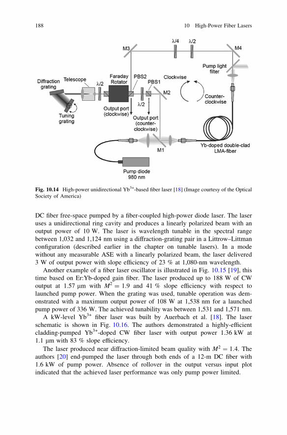
DC fiber free-space pumped by a fiber-coupled high-power diode laser. The laseruses a unidirectional ring cavity and produces a linearly polarized beam with anoutput power of 10 W. The laser is wavelength tunable in the spectral rangebetween 1,032 and 1,124 nm using a diffraction-grating pair in a Littrow–Littmanconfiguration (described earlier in the chapter on tunable lasers). In a modewithout any measurable ASE with a linearly polarized beam, the laser delivered3 W of output power with slope efficiency of 23 % at 1,080-nm wavelength.

Another example of a fiber laser oscillator is illustrated in Fig. 10.15 [19], thistime based on Er:Yb-doped gain fiber. The laser produced up to 188 W of CWoutput at 1.57 lm with M2 = 1.9 and 41 % slope efficiency with respect tolaunched pump power. When the grating was used, tunable operation was dem-onstrated with a maximum output power of 108 W at 1,538 nm for a launchedpump power of 336 W. The achieved tunability was between 1,531 and 1,571 nm.

A kW-level Yb3+ fiber laser was built by Auerbach et al. [18]. The laserschematic is shown in Fig. 10.16. The authors demonstrated a highly-efficientcladding-pumped Yb3+-doped CW fiber laser with output power 1.36 kW at1.1 lm with 83 % slope efficiency.

The laser produced near diffraction-limited beam quality with M2 ¼ 1:4. Theauthors [20] end-pumped the laser through both ends of a 12-m DC fiber with1.6 kW of pump power. Absence of rollover in the output versus input plotindicated that the achieved laser performance was only pump power limited.

Fig. 10.14 High-power unidirectional Yb3+-based fiber laser [18] (Image courtesy of the OpticalSociety of America)

188 10 High-Power Fiber Lasers

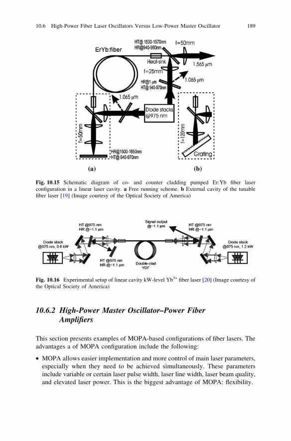
10.6.2 High-Power Master Oscillator–Power FiberAmplifiers

This section presents examples of MOPA-based configurations of fiber lasers. Theadvantages a of MOPA configuration include the following:

• MOPA allows easier implementation and more control of main laser parameters,especially when they need to be achieved simultaneously. These parametersinclude variable or certain laser pulse width, laser line width, laser beam quality,and elevated laser power. This is the biggest advantage of MOPA: flexibility.

Fig. 10.15 Schematic diagram of co- and counter cladding pumped Er:Yb fiber laserconfiguration in a linear laser cavity. a Free running scheme. b External cavity of the tunablefiber laser [19] (Image courtesy of the Optical Society of America)

Fig. 10.16 Experimental setup of linear cavity kW-level Yb3+ fiber laser [20] (Image courtesy ofthe Optical Society of America)

10.6 High-Power Fiber Laser Oscillators Versus Low-Power Master Oscillator 189

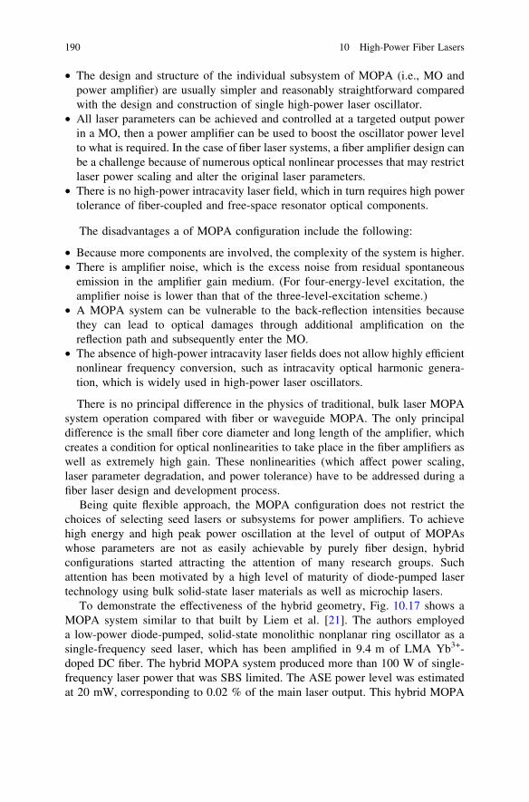
• The design and structure of the individual subsystem of MOPA (i.e., MO andpower amplifier) are usually simpler and reasonably straightforward comparedwith the design and construction of single high-power laser oscillator.

• All laser parameters can be achieved and controlled at a targeted output powerin a MO, then a power amplifier can be used to boost the oscillator power levelto what is required. In the case of fiber laser systems, a fiber amplifier design canbe a challenge because of numerous optical nonlinear processes that may restrictlaser power scaling and alter the original laser parameters.

• There is no high-power intracavity laser field, which in turn requires high powertolerance of fiber-coupled and free-space resonator optical components.

The disadvantages a of MOPA configuration include the following:

• Because more components are involved, the complexity of the system is higher.• There is amplifier noise, which is the excess noise from residual spontaneous

emission in the amplifier gain medium. (For four-energy-level excitation, theamplifier noise is lower than that of the three-level-excitation scheme.)

• A MOPA system can be vulnerable to the back-reflection intensities becausethey can lead to optical damages through additional amplification on thereflection path and subsequently enter the MO.

• The absence of high-power intracavity laser fields does not allow highly efficientnonlinear frequency conversion, such as intracavity optical harmonic genera-tion, which is widely used in high-power laser oscillators.

There is no principal difference in the physics of traditional, bulk laser MOPAsystem operation compared with fiber or waveguide MOPA. The only principaldifference is the small fiber core diameter and long length of the amplifier, whichcreates a condition for optical nonlinearities to take place in the fiber amplifiers aswell as extremely high gain. These nonlinearities (which affect power scaling,laser parameter degradation, and power tolerance) have to be addressed during afiber laser design and development process.

Being quite flexible approach, the MOPA configuration does not restrict thechoices of selecting seed lasers or subsystems for power amplifiers. To achievehigh energy and high peak power oscillation at the level of output of MOPAswhose parameters are not as easily achievable by purely fiber design, hybridconfigurations started attracting the attention of many research groups. Suchattention has been motivated by a high level of maturity of diode-pumped lasertechnology using bulk solid-state laser materials as well as microchip lasers.

To demonstrate the effectiveness of the hybrid geometry, Fig. 10.17 shows aMOPA system similar to that built by Liem et al. [21]. The authors employeda low-power diode-pumped, solid-state monolithic nonplanar ring oscillator as asingle-frequency seed laser, which has been amplified in 9.4 m of LMA Yb3+-doped DC fiber. The hybrid MOPA system produced more than 100 W of single-frequency laser power that was SBS limited. The ASE power level was estimatedat 20 mW, corresponding to 0.02 % of the main laser output. This hybrid MOPA

190 10 High-Power Fiber Lasers

configuration preserves excellent beam quality, a high degree of polarization, andsingle-frequency nature of the seed laser. The system is scalable to a power levelof more than 200 W.

Figure 10.18 shows an example of high-power pulsed MOPA design in which aYb3+-doped DC fiber amplifier was used by Dupriez et al. [22]. The MOPAconsists of a current modulated seed laser diode, three-stage preamplifier, and a

Double clad LMA gain fiber

Single frequencyNPRO or Microchip

Laser

Optical Isolator

Output

Fiber coupled,multimode pump

diode lasers

Dichroicmirror

LensLens Lens

Optical Isolator

Fig. 10.17 Schematic setup of the single-frequency master oscillator–fiber power amplifier.LMA large mode area, NPRO nonplanar ring oscillator

Fig. 10.18 Experimental setup of a 321-W average power pulse MOPA-based Yb3+ fiber laser[22]. CP cladding pumped, CFBG chirped fiber Bragg grating (Image courtesy of the OpticalSociety of America)

10.6 High-Power Fiber Laser Oscillators Versus Low-Power Master Oscillator 191

high-power amplifier. In total, 492 lW of diode laser power is injected into thethree-stage preamplifier and is boosted to 2 W of output power before it enters thelast high-power amplifier stage. The final high-power amplifier is counter-pumpedwith a high-power 975-nm diode laser and produces 321 W of average power at1,060-nm wavelength. The laser demonstrates 20-ps pulses at a 1-GHz repetitionrate. Despite high peak power of the laser pulses, the observed SPM was moderateand no Raman scattering has been detected at the output of fiber power amplifier.

Another example of a high peak power nanosecond MOPA was developed byNufern [23], as shown in Fig. 10.19. The authors [23] demonstrated a monolithiclinearly-polarized pulsed Yb3+-doped fiber laser, with [10 kW peak power, tun-able pulse duration of 2 ns to 0.2 ls, tunable repetition rate of 50 kHz to 50 MHz,and 50 W average power in a diffraction-limited, linearly polarized, and stabilized0.8 nm line-width output beam operating at 106 nm.

A high average power, femtosecond Yb3+ fiber MOPA was reported byRoser et al. [24]. Using the fiber laser schematic shown in Fig. 10.20, the authors[24] demonstrated 90.4 W average power of 500-fs pulses while the laser operatedat a 0.9 MHz pulse repetition rate. The femtosecond pulse peak power from such afiber laser system reached the 200-MW level.

Fig. 10.19 Linearly polarized, nanosecond fiber laser design [23]. LMA large mode area,MO master oscillator PM, polarization maintained; SM, single mode. (Image courtesy of Theinternational Society for Optics and Photonics (SPIE).)

Fig. 10.20 Experimental setup of a high average power femtosecond MOPA system [24]. AOMacousto-optical modulator, OI optical isolator (Image courtesy of SPIE)

192 10 High-Power Fiber Lasers

The MOPA configuration has also been employed for resonantly pumpedEr-only high-power amplifiers. The approach is considered to be a power-scalable,eye-safe, highly efficient alternative to existing high-power Yb3+ fiber lasers in the1-lm range of the optical spectrum). Dubinskii et al. [25] implemented the high-power cladding-pumped Yb3+-free Er3+ amplifier system resonantly pumped at1,480 and 1,530 nm, as shown in Fig. 10.21. The authors [25] designed a single-frequency Er3+ fiber laser using a single-frequency diode laser as a MO, onepreamplifier, and a high-power cladding-pumped amplifier. Using a Liekki Er3+-doped 20/125 LMA gain fiber in a booster stage, the authors achieved 46 % slopeefficiency versus absorbed power when cladding pumped with 1,520–1,530-nmfiber-coupled laser diodes, as well as more than 9 W of CW optical power withdiffraction-limited beam quality at a 1,570-nm wavelength.

An interesting approach to scale output power of single-frequency fiber laserswas introduced by Zeringue et al. [26]. The authors used monolithic PM Yb3+-doped fiber amplifier seeded with a combination of broad (tunable in the1,035–1,045-nm range) and single-frequency (1,065-nm) laser signals, as shown inFig. 10.22. This two-tone concept was used in conjunction with externally appliedor intrinsically formed thermal gradients to achieve SBS suppression factors of upto 7 dB in a 7-m-long Yb3+-doped 25/400 fiber. Achieved output power of the

Fig. 10.21 Schematic of resonantly pumped Yb3+-free, Er3+ fiber amplifier [26]. LMA largemode area (Image courtesy of SPIE)

10.6 High-Power Fiber Laser Oscillators Versus Low-Power Master Oscillator 193

single-frequency laser ranged from 80 to 203 W, with slope efficiencies of70–80 %. Using an external thermal gradient, the authors measured 100 kHznominal line-width at 203 W of output power of the laser.

Goodno et al. [27] built a four-stage, Tm3+-doped fiber amplifier chain thatemitted 608 W of single-frequency output power. The laser showed an optical gainof 53 dB, 54 % slope efficiency, and beam quality with M2 of 1.05, as shown inFig. 10.23. The output power was limited by available pump power and showednow saturation with increasing pump power level. The laser system preserved theinput \5-MHz line width, imposing negligible phase noise above 3 kHz.A comparison of the measured SBS limit as well as analytically analyzed thermal

Fig. 10.22 Experimental setup used in Zeringue et al. [26]. PD photodiode, ISO isolator; PMpower meter, OSA optical spectrum analyzer, WDM wavelength-division multiplexer. The ASEfilter is used to suppress noise introduced by the broadband laser [23] (Image courtesy of SPIE)

Fig. 10.23 Experimental setup of a four-stage, single-frequency Tm3+-fiber laser MOPA [27].ASE, amplified spontaneous emission; DFB, distributed feedback laser. (Image courtesy of Theinternational Society for Optics and Photonics (SPIE).)

194 10 High-Power Fiber Lasers

limit suggests a maximum possible achievable single-frequency power of*750 W from this fiber laser, scalable to the 1-kW level [27].

It is important to note that selection of the approach used in the design anddevelopment of a high-power fiber laser system depends on many factors, whichhave to be taken into consideration during the decision-making process in selectinga schematic. These factors include the fundamental allowance of the theoreticalmodeling, required flexibility of the targeted output laser parameters, and allocatedcost. This decision also involves information on the availability of the fiber-coupledand free-space optical components used in both MOPA and oscillator systems.

10.7 Beam Combining of High-Power Fiber Lasers

The unique advantages of fiber laser systems—high efficiency, high beam quality,relaxed thermal management issues, and low cost of ownership—helped them tocapture several industrial markets as well as some military applications. The latterapplications, however, requires a high level of average or CW powers in the orderof 50–100 kW, while at the same time maintaining high beam quality ofdiffraction-limited operation.

Two ways to scale the power of laser systems have been implemented intopractice: (a) scaling power of an individual oscillator without degradation ofimportant laser parameters and (b) beam combination of already constructedlasers. By pushing the capabilities to the maximum possible level, both methodscan usually be implemented by researchers and engineers. This section reviews themain approaches for high-power beam combing.

The most important parameters of the individual high-power fiber laser sourcesand their control when considering laser beam combinations include wavelengthcontrol, line-width control, and polarization control. By exploring these laserparameters, one may achieve different beam combinations to scale the fiber lasersystem output power. By combining several laser beams while preserving the beamparameter product (i.e., the productof the beam diameter and the angleofdivergence),one may not only scale the output power but also increase the beam brightness.

There are three main approaches for beam combining to increase the outputlaser beam power (see [28] for a review):

1. Spectral beam combining (sometimes called wavelength beam combining, orWBC).

2. Coherent beam combining.3. Side-by-side beam combining.

The traditional polarization beam combining technique (PBC; see Fig. 10.24),which combines two linear polarized beams and uses polarization beam splitters/combiners, increases brightness. However, it also results in an unpolarized outputbeam and therefore cannot be used for repeatable beam combiners based on thepolarization control principle. Another reason that restricts the use of PBC in

10.6 High-Power Fiber Laser Oscillators Versus Low-Power Master Oscillator 195

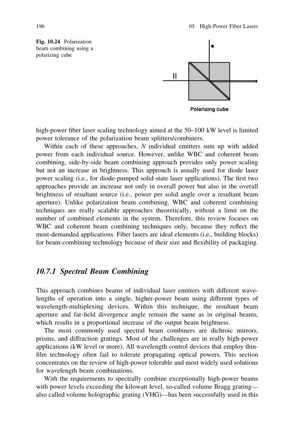
high-power fiber laser scaling technology aimed at the 50–100 kW level is limitedpower tolerance of the polarization beam splitters/combiners.

Within each of these approaches, N individual emitters sum up with addedpower from each individual source. However, unlike WBC and coherent beamcombining, side-by-side beam combining approach provides only power scalingbut not an increase in brightness. This approach is usually used for diode laserpower scaling (i.e., for diode-pumped solid-state laser applications). The first twoapproaches provide an increase not only in overall power but also in the overallbrightness of resultant source (i.e., power per solid angle over a resultant beamaperture). Unlike polarization beam combining, WBC and coherent combiningtechniques are really scalable approaches theoretically, without a limit on thenumber of combined elements in the system. Therefore, this review focuses onWBC and coherent beam combining techniques only, because they reflect themost-demanded applications. Fiber lasers are ideal elements (i.e., building blocks)for beam-combining technology because of their size and flexibility of packaging.

10.7.1 Spectral Beam Combining

This approach combines beams of individual laser emitters with different wave-lengths of operation into a single, higher-power beam using different types ofwavelength-multiplexing devices. Within this technique, the resultant beamaperture and far-field divergence angle remain the same as in original beams,which results in a proportional increase of the output beam brightness.

The most commonly used spectral beam combiners are dichroic mirrors,prisms, and diffraction gratings. Most of the challenges are in really high-powerapplications (kW level or more). All wavelength control devices that employ thin-film technology often fail to tolerate propagating optical powers. This sectionconcentrates on the review of high-power tolerable and most widely used solutionsfor wavelength beam combinations.

With the requirements to spectrally combine exceptionally high-power beamswith power levels exceeding the kilowatt level, so-called volume Bragg grating—also called volume holographic grating (VHG)—has been successfully used in this

Fig. 10.24 Polarizationbeam combining using apolarizing cube

196 10 High-Power Fiber Lasers

application [29]. Figure 10.25a shows a schematic view of a spectral beam-combining technique using VHG (For comparison, diffraction-grating WBC isshown in Fig. 10.25b).

Being a repeatable device (i.e., the device allows a consequent beam combi-nation of a theoretically unlimited number of single beams), VHG are the mostwidely used multiplexers, particularly for high-power fiber laser systems [29].Highly efficient diffractive Bragg gratings in photo-thermo-refractive (PTR)inorganic glass have been applied for high-power laser systems [30, 31]. PTR glassdemonstrates high diffraction efficiency ([95 %) in both the transmitting andreflecting types of Bragg gratings. This material demonstrates exceptional thermaland mechanical stability as well as high optical quality. Ciapurin et al. [31]reported low PTR absorption in of 1 lm spectral range with power densitytolerance of 100 kW/cm2.

10.7.2 Volume Holographic Grating

Because of the very important role that VHG plays in the beam combinationtechnology, it is useful here to present some overview on general properties ofVHG [32–36]. VHG is a thick Bragg diffraction grating recorded in a PTR glass(Note that VHG can be fabricated in other materials, such as photo-refractivecrystals or gelatin). In addition to WBC applications, VHG are widely used forhighly efficient spectral narrowing of high- and low-power diode lasers. Generally,VHGs can be categorized into transmission and reflection types (see Fig. 10.26),depending on the direction of incident and diffracted light.

The simplest nonslanted transmission and reflection gratings demonstrate thecommon characteristics of the VHG. Consider a nonslanted transmission grating

Fig. 10.25 Spectral beamcombining using a volumeholographic (Bragg) grating(a) and a diffractiongrating (b)

10.7 Beam Combining of High-Power Fiber Lasers 197

with index modulation Dn, with typical values between ð100 300Þ � 10�6 andthickness d. The diffraction efficiency is defined as the ratio between the diffractedintensity and the incident intensity, without considering absorption and Fresnelreflections at the surfaces. When the Bragg condition is satisfied for wavelengthkB, the diffraction efficiency effB is given as:

effB ¼ sin2 p� Dn� d

kB cos Hn

� �

ð10:52Þ

where hn is the incident angle inside the medium of index n. When the gratingstrength Dn increases from zero, the diffraction efficiency increases from 0 to100 % when:

Dn ¼ kB cos Hn

2dð10:53Þ

For even stronger gratings, the diffraction efficiency effB will decrease from100 % because the diffracted beam is diffracted again by the same grating andcoupled back into the original incident beam.

Due to the volume hologram, Bragg-matching condition VHGs have highlysensitive wavelength and angle selectivity. Consider a weak nonslanted trans-mission grating (i.e., effB \100 %). When the incident wavelength k is differentthan the Bragg wavelength kB, the diffraction efficiency eff(k) can be approxi-mated as a typical sinc function:

effðkÞ ¼ effB �sin kB�k

Dk

� �

kB�kDk

� �

" #2

ð10:54Þ

where Dk is the wavelength deviation at the first null, as shown in Fig. 10.27 (top).

Fig. 10.26 Two types ofvolume holographic grating(VHG): reflectionholographic grating (left) andtransmission holographicgrating (right) (Imagecourtesy of Ondax)

198 10 High-Power Fiber Lasers

Similarly when the incident angle in air h is different than the Bragg angle HB,the diffraction efficiency effB can be approximated as a typical sinc function:

effðHÞ ¼ effB �sin HB�H

DH

� �

HB�HDH

� �

" #2

ð10:55Þ

where DH is the incident angle deviation at the first null, as shown in Fig. 10.27(right).

Using this analysis, one can calculate the required Bragg grating parameters forthe incident spectrum of a multichannel laser system. Calculation and manufac-turability analyses show that practical minimum spectral separation of individuallaser channels should be 2 nm or more to avoid cross-talk. For a more detailedtheory of VHG, please see Ref. [36].

Fig. 10.27 Typicalwavelength and angledependence curves forvolume holographic gratings(VHGs). When the Braggcondition is equal towavelengthkB and incidentangle HB, the diffractionefficiency is effB (the centralmaximum on the figures)

10.7 Beam Combining of High-Power Fiber Lasers 199

VHG can be used not only in spectral but in coherent combiners as well. VHGsrecorded in glass have been first suggested for use in coherent coupling of diodelasers in Refs. [37, 38]. The basic idea of this approach is to use volume Bragggratings to create extremely dispersive external resonators for coherently com-bining individual lasers. The VHG is acting within this approach as a commonoutput coupler. Venus et al. [37, 38] coherently coupled two 980-nm diode lasersand produced single wavelength output for both diodes with spectral width nar-rowed to \30 pm. Similar technology can be applied for high-power fiber lasersusing coherent beam combining and is potentially capable of achieving 100-kWlevel of coherent fiber laser radiation.

10.7.3 Coherent Beam Combining

Coherent beam combining adds beams emerging from different individual lasersources (or gain sections) passively or actively phase-locked to each other, usuallyby some intracavity element or external force to each of the laser resonators (i.e.,compensation of phase errors using phase-conjugate elements such as SBS andphase detection with active compensation), with beams interacting externally tothe individual laser. In other words, this beam-combining approach forces indi-vidual sources to operate with the same frequency spectrum and with the samephase. Using a spatial overlapping of individual emitters’ electrical fields, coherentbeam combining results in power scaling of the output laser emission.

There are two basic approaches for coherent laser coupling. The first is to injectcoherent radiation to the separate lasers and force them to emit coherently. Thisapproach allows for the oscillation of all components of the system in the samemode. However, this approach involves certain risk in systems such as MOPAbecause back-seeding power may produce optical damage to all in-line lasercomponents; it also requires subsequent coherent coupling of the individual laserseven if individual locking is successful.

The second approach is to design a multichannel high-power laser resonator thatprovides coherent emission of all its components. This approach allows phase controlto be obviated in the channels, but the main problem that prevents stable and efficientcoupling is a tendency of a multichannel system to switch between different modes ofa complex laser resonator. However, if one achieves high spectral and angle selec-tivity in the combining device, the second approach may become very effective.

For example, consider two designs. In the approach shown in Fig. 10.28, aso-called all-fiber approach for coherent beam combining was proposed [39].Here, the authors demonstrated the use of half of a fused-taper single-mode fibercoupler as an output mirror–beam combiner for two fiber lasers. The approach canbe used for combining high-power fiber lasers. By tuning one of the fiber laser’sBragg grating mirrors, the authors observed fiber laser injection locking. Theydemonstrated both spatial and spectral combination of two fiber lasers. Later,a similar approach (see Fig. 10.29) was implemented by another group [40], whodemonstrated highly efficient coherent beam combining of N fiber lasers byY-shaped fused fiber couplers. The authors [40] obtained 2.65 W of combined

200 10 High-Power Fiber Lasers

fiber laser emission by combining eight erbium-doped fiber lasers with an 85 %combining efficiency.

For the multielement intracavity beam combination, an interesting design hasbeen suggested and implemented [41], as shown in Fig. 10.30. The authors usedthe design to scale the power of the fiber laser system consisting of large numbersof elements while maintaining good beam quality. As one can see from Fig. 10.30,the authors used a MOPA configuration as a building block of the system, whichdefined temporal and spectral characteristics of the individual source.

Each fiber oscillator is placed at the focal plane of the MO array lens; therefore,every oscillator radiation is collimated before falling onto the diffraction grating[41]. The end mirror and grating in the MO array section act as a complex mirror

Fig. 10.28 Experimental setup. OSA optical spectrum analyzer, WDM wavelength-divisionmultiplexer [39] (Image courtesy of the Optical Society of America)

Fig. 10.29 a Experimental setup and b power evolution of the N = 8 fiber laser coherent array[40]. WDM wavelength-division multiplexer; PC, polarization controller; EDF,erbium dopedfiber; FC, fiber connector, APC, angle-polished connector. (Imagecourtesy of the Optical Societyof America.)

10.7 Beam Combining of High-Power Fiber Lasers 201

and provide feedback at different wavelengths for each fiber oscillator. Subse-quently reflected emissions then seed each oscillator on its individual wavelength,which then follow with its own amplifier. Using a similar approach, amplifiedbeams are combined on the second diffraction grating; after recollimation, they arecoupled out of the system as an output beam (Fig. 10.30).

Shay et al. [42] experimentally demonstrated an original technique for coherentbeam combining of laser beams. Using a so-called Locking of Optical Coherenceby Single-detector Electronic-frequency Tagging (LOCSET), the authors achievedphase locking of an array of five 145-W fiber amplifiers. The resultant laser beamproduced a record 725-W optical power as a result of coherent beam combination(see Fig. 10.31).

As shown in Fig. 10.31, the MO is coupled into two single-mode PM 1 9 8power splitters, which have separate phase modulators in each of the eight legs.The output of the modulators is coupled into eight single-mode PM optical fibers.

Fig. 10.30 MOPA implementation of a wavelength beam combining system. Each element inthe master oscillator operates at a unique wavelength determined by the grating. Part of the lightfrom each oscillator element is used to seed its own amplifier and the amplifier outputs arecombined with an identical transform lens and grating [41] (Image courtesy of the OpticalSociety of America)

Fig. 10.31 Block diagram ofLocking of OpticalCoherence by Single-detectorElectronic-frequencyTagging (LOCSET) beam-combining experiment [42].PM phase modulator, PDphotodetector (Imagecourtesy of SPIE)

202 10 High-Power Fiber Lasers

After each modulator, the light gets coupled into fiber amplifiers. Each amplifieroutput is collimated by the lens optics and, after passing through a beam splitter, isdirected onto a single photodetector by a focusing lens. A small-amplitude radio-frequency (RF) phase modulator is applied to each of the phase modulators at aunique individual RF frequency. The photodetector produces a photocurrent thatcontains the RF phase modulation frequencies of each beam. In addition, theamplitude of each RF frequency component contains the optical phase error signalfor each of the array elements. By electronically extracting the optical phase errorfor each array element and feeding it back to the corresponding phase modulator,the authors [42] were able to lock each array element to the same phase as theother element in the system.

Unlike other approaches, this technique does not require a reference beam.Avoiding the use of an external reference beam from the electronic phase-lockingsystem simplifies the optical alignment and allows the usage of a single photo-detector for the whole system of N combining channels. Mechanical andenvironmental tolerance of the approach may lead to reliable and practical multi-kilowatt laser systems.

An interesting approach has been demonstrated by Fridman et al. [43], whoachieved simultaneous coherent and spectral beam combination in one system(Fig. 10.32). Coherent combination was achieved in the horizontal direction usingan interferometric combiner, while spectral combining was implemented in thevertical direction using linear diffraction grating. The authors [43] experimentallydemonstrated a combining efficiency of more than 80 % with resultant beamquality of M2 = 1.15.

Ludewigt et al. [44] demonstrated the spectral beam combination of four narrowline-width LMA photonic crystal fiber amplifiers (Fig. 10.33). Each individualbeam had a spectral width of *90 pm at an output power of *2.1 kW and a beamquality of M2 * 4. The polarization-independent grating allowed an efficiency of99 %. The combined beam has an average power of 8.2 kW (pump power limited)with a good beam quality, practically preserving the beam quality of the individualfiber amplifiers.

Drachenberg et al. [45] presented high-power, high-spectral-density beamcombining using VBG of five 150-W beams with a spectral separation of 0.25 nm

Fig. 10.32 A schematic usedfor simultaneous coherentand spectral combination offour fiber laser beams [43].FBG fiber Bragg grating(Image courtesy of SPIE)

10.7 Beam Combining of High-Power Fiber Lasers 203

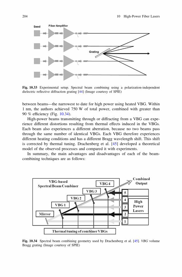
between beams—the narrowest to date for high power using heated VBG. Within1 nm, the authors achieved 750 W of total power, combined with greater than90 % efficiency (Fig. 10.34).

High-power beams transmitting through or diffracting from a VBG can expe-rience different distortions resulting from thermal effects induced in the VBGs.Each beam also experiences a different aberration, because no two beams passthrough the same number of identical VBGs. Each VBG therefore experiencesdifferent heating conditions and has a different Bragg wavelength shift. This shiftis corrected by thermal tuning. Drachenberg et al. [45] developed a theoreticalmodel of the observed processes and compared it with experiments.

In summary, the main advantages and disadvantages of each of the beam-combining techniques are as follows:

Fig. 10.33 Experimental setup. Spectral beam combining using a polarization-independentdielectric reflective diffraction grating [44] (Image courtesy of SPIE)

Fig. 10.34 Spectral beam combining geometry used by Drachenberg et al. [45]. VBG volumeBragg grating (Image courtesy of SPIE)

204 10 High-Power Fiber Lasers

10.7.3.1 Spectral Beam Combining

• Does not require coherency of individual beams to be combined beams.• Because of an increased spectral width of the resultant beam, the spectral bright-

ness (i.e., brightness per unit spectral bandwidth ½W=cm2 � steradian� nm�) isreduced.

• Reasonably preserves the original beam quality.• Is an additive technique in terms of power scaling (i.e., except for the power

reduction, failure of one source does not affect the performance of other sourcesand the resultant beam).

• Requires narrower possible line-width of individual laser emitters, especially ifa large number of beams has to be combined. In turn, this often requires single-frequency operation of individual lasers, which may be a challenging task—particularly for high-power systems due to being detrimental for power-scalingnonlinear optical processes.

10.7.3.2 Coherent Beam Combining

• Often requires individual sources to share laser resonator components to achievecoherency of the output combined beam, which in turn complicates the wholesystem design. Particularly, increased intracavity power applies additionalpower tolerance requirements to laser cavity optics.

• Usually demonstrates increased spectral brightness because the technique eitherpreserves or even reduces individual laser spectral line-width while addingoptical power in the resultant beam.

• Reasonably preserves the original beam quality.• Not an additive technique in terms of power scaling (i.e., failure of one source

affects the performance of other sources and the resultant beam, including beamquality).

• Does not necessary require single frequency (i.e., very narrow spectral line-width) of individual laser emitters.

At the current stage of technology development (except for the cases when theresultant output beam spectral bandwidth is of concern, such as in the case ofnonlinear frequency conversion or applications where long coherence length isrequired), spectral beam combing shows great promise for the power scaling offiber lasers.

10.7 Beam Combining of High-Power Fiber Lasers 205

References

1. T.A. Parthasarathy, R.S. Hay, G.E. Fair, F.K. Hopkins, Predicted performance limits ofyttrium aluminum garnet fiber lasers. Opt. Eng. 49(9), 094302 (2010)

2. A. Wetter, M. Faucher, M. Lovelady, F. Seguin, Tapered fused-bundle splitter capable of1 kW CW operation. Proc. SPIE 6453, 64530I.1–64530I.10 (2007)

3. J.P. Koplow, S.W. Moore, D.A.V. Kliner, A new method for side pumping of double-cladfiber sources. IEEE J. Quantum Electron. 39(4), 529–540 (2003)

4. D.J. Ropin, L. Goldberg, High efficiency side-coupling of light into optical fibres usingimbedded v-grooves. Electron. Lett. 31(25), 2204–2205 (1995)

5. H. Weber, W. Luthy, H.P. Weber, V. Neuman, H. Berthou, G. Kotrotsios, A longitudinal andside-pumped single transverse mode double-clad fiber laser with a special silicone coating.Opt. Commun. 115, 99–104 (1995)

6. J.M. Fini, Bend distortion in large-mode-area amplifier fiber design, Proc. SPIE 6781 (2007)7. B.Y. Zel’Dovich, N.F. Pilipetsky, V.V. Shkunov, Principles of Phase Conjugation (Springer

Series in Optical Sciences, Berlin, 1985), p. 250 (Hardcover)8. G.W. Faris et al., High–resolution stimulated Brillouin gain spectroscopy in glasses and

crystals. JOSA B 10(4), 587–599 (1993)9. G.P. Agrawal, Nonlinear Fiber Optics, 3rd edn. (Academic Press, New York, 2001), p. 466

10. R.R. Alfano et al., Cross-phase modulation and induced focusing due to optical nonlinearitiesin optical fibers and bulk materials. J. Opt. Soc. Am. B. 6(4), 824–829 (1989)

11. G.A. Askarian, Effect of the gradient of a strong electromagnetic ray on electrons and atoms.Zh. Eksp. Teor. Fiz. 42, 1361–1570 (1962)

12. G.M. Zverev, V.A. Pashkov, Self-focusing of laser radiation in solid dielectrics. Sov. Phys.JETP 30(4), 616–621 (1970)

13. R.Y. Chiao, E. Garmire, C.H. Townes, Self-trapping of optical beams. Phys. Rev. Lett. 13,479–482 (1964)

14. S.A. Akhmanov, A.P. Sukhorukov, R.V. Khokhlov, Self focusing and diffraction of light in anonlinear medium. Sov. Phys. Uspekhi 93, 609–636 (1968)

15. V.I. Bespalov, V.I. Talanov, Filamentary structure of light beams in nonlinear liquids. JETPLett. 3, 307–310 (1966)

16. A.A. Mak, L.N. Soms, V.A. Fromzel, V.E. Yashiin, Lasers Based on Neodymium Glass(Nauka, Moscow, 1990), pp. 1–288

17. S.A. Akhmanov, A.P. Sukhorukov, R.V. Khokhlov, Self-focusing and diffraction of light in anonlinear medium. Phys. Uspekhi 10, 609–636 (1968)

18. M. Auerbach, P. Adel, D. Wandt, C. Fallnich, S. Unger, S. Jetschke, H. Mueller, 10 Wwidely tunable narrow linewidth double-clad fiber ring laser. Opt. Express 10, 139–144(2002)

19. D.Y. Shen, J.K. Sahu, W.A. Clarkson, Highly efficient Er, Yb-doped fiber laser with 188 Wfree-running and [100 W tunable output power. Opt. Express 13, 4916–4921 (2005)

20. Y. Jeong, J. Sahu, D. Payne, J. Nilsson, Ytterbium-doped large-core fiber laser with 1.36 kWcontinuous-wave output power. Opt. Express 12, 6088–6092 (2004)

21. A. Liem, J. Limpert, H. Zellmer, A. Tünnermann, 100-W single-frequency master-oscillatorfiber power amplifier. Opt. Lett. 28, 1537–1539 (2003)

22. P. Dupriez, A. Piper, A. Malinowski, J.K. Sahu, M. Ibsen, Y. Jeong, L.M.B. Hickey, M.N.Zervas, J. Nilsson, D.J. Richardson, 321 W average power, 1 GHz, 20 ps, 1060 nm pulsedfiber MOPA source, in Optical Fiber Communication Conference and Exposition and TheNational Fiber Optic Engineers Conference, Technical Digest (CD) (Optical Society ofAmerica, 2005), paper PDP3

23. V. Khitrov, B. Samson, D. Machewirth, K. Tankala, 50 W single-mode linearly polarizedhigh peak power pulsed fiber laser with tunable ns-ls pulse durations and kHz-MHzrepetition. Proc. SPIE 6873, 68730C1–68730C6 (2008)

206 10 High-Power Fiber Lasers

24. F. Roser, D. Schimpf, O. Schmidt, B. Ortac, K. Rademaker, J. Limpert, A. Tunnermann,90 W average power high energy femtosecond fiber laser system. Proc. SPIE 6453,645310.1–645310.4 (2007)

25. M. Dubinskii, V. Ter-Mikirtychev, J. Zhang, I. Kudryashov, Yb-free, SLM EDFA:comparison of 980-, 1470- and 1530-nm excitation for the core-and clad-pumping. Proc.SPIE 6952, 695205 (2008)

26. C. Zeringue, I. Dajani, C. Vergien, C. Robin, Pump limited 203 W monolithic singlefrequency fiber amplifier: a two-tone approach. Proc. SPIE 7914, paper 7914-115 (2011)

27. G.D. Goodno, L.D. Book, J.E. Rothenberg, 600-W, single-mode, single-frequency thuliumfiber laser amplifier. Proc. SPIE 7195, paper 71950Y-1-10 (2009)

28. T.Y. Fan, Laser beam combining for high-power, high radiance sources. IEEE J. Sel. Top.Quantum Electron. 11, 567–577 (2005)

29. I. Ciapurin, L. Glebov, E. Rotari, V. Smirnov, Spectral beam combining by PTR Bragggratings, in Proceedings of Solid State and Diode Lasers Technical Review (SSDLTR) (2003),pp. HPFib—4

30. L.B. Glebov, V.I. Smirnov, M.C. Stickley, I.V. Ciapurin, Laser weapons technology III. Proc.SPIE 4724, 101–109 (2002)

31. I.V. Ciapurin, L.B. Glebov, C.M. Stickley, in Proceedings of Solid State and Diode LasersTechnical Review. Albuquerque, Paper HPFIB4 (2002)

32. O. Andrusyak, D. Drachenberg, V. Smirnov, G. Venus, L. Glebov, Fiber laser system withkW-level spectrally-combined output, in 21st Annual Solid State and Diode LaserTechnology Review, SSDLTR-2008 Technical Digest, Albuquerque, NM (June 2008), pp. 2–6

33. O. Andrusyak, I. Ciapurin, V. Smirnov, G.Venus, N. Vorobiev, L. Glebov, External andcommon-cavity high spectral density beam combining of high power fiber lasers, fiber lasersV: technology, systems, and applications, ed. by J. Broeng, C. Headley, Proceedings of SPIE,vol. 6873 (2008), p. 685314

34. A. Sevian, O. Andrusyak, I. Ciapurin, G. Venus, V. Smirnov, L. Glebov, Efficient powerscaling of laser radiation by spectral beam combining. Opt. Lett. 33, 384–386 (2008)

35. A. Sevian, O. Andrusyak, I. Ciapurin, G. Venus, V. Smirnov, L. Glebov, Efficient powerscaling of laser radiation by spectral beam combining: erratum. Opt. Lett. 33, 760 (2008)

36. I.V. Ciapurin, L.B. Glebov, V.I. Smirnov, Modeling of Gaussian beam diffraction on volumeBragg gratings in PTR glass. Proc. SPIE 5742, 183–194 (2005), See also Introduction toVolume Holographic Gratings (VHG), Ondax, white paper (www.ondax.com)

37. G. Venus, A. Sevian, V. Smirnov, L. Glebov, Stable coherent coupling of laser diodes by avolume Bragg grating in photothermorefractive glass. Opt. Lett. 31, 1453–1455 (2006)

38. G. Venus, A. Sevian, L. Glebov, in Stable Coherent Coupling of Laser Diodes by a VolumeBragg Rating in PTR Glass. High-Power Diode Laser Technology and Applications IV, ed.by M. Zediker, Proceedings of SPIE, vol. 6104 (2006), p. 61040S

39. V.A. Kozlov, J. Hernández-Cordero, T.F. Morse, All-fiber coherent beam combining of fiberlasers. Opt. Lett. 24, 1814–1816 (1999)

40. A. Shirakawa, K. Matsuo, K. Ueda, Fiber laser coherent array for power scaling, bandwidthnarrowing and beam direction control, in Advanced Solid-State Photonics, Technical Digest(Optical Society of America, 2005), paper MC3, pp. 553–558

41. S.J. Augst, J.K. Ranka, T.Y. Fan, A. Sanchez, Beam combining of ytterbium fiber amplifiers.J. Opt. Soc. Am. B 24, 1707–1715 (2007)

42. T. Shay, J. Baker, A. Sanchez, C. Robin, C. Vergien, C. Zeringue, D. Gallant, C. Lu,B. Pulford, T. Bronder, A. Lucero, in High-Power Phase Locking of a Fiber Amplifier Array,Fiber Lasers VI: Technology, Systems, and Applications, ed. by D.V. Gapontsev,D.A. Kliner, J.W. Dawson, K. Tankala, Proceedings of SPIE, vol. 7195, 71951M

43. M. Fridman, V. Eckhouse, N. Davidson, A.A. Friesem, Simultaneous coherent and spectraladdition of fiber lasers. Opt. Lett. 33, 648–650 (2008)

44. K. Ludewigt, M. Gowin, E.T Have1, M. Jung, C. Wirth, O. Schmidt, I. Tsybin, T. Schreiber,R. Eberhardt, J. Limpert, A. Tünnermann, High brightness spectral beam combining to8.2 kW. Proc. SPIE 7914, Paper 7914-115 (2011)

References 207

45. D. Drachenberg, I. Divliansky, V. Smirnov, G. Venus, L. Glebov, High power spectral beamcombining of fiber lasers with ultra high spectral density by thermal tuning of volume bragggratings. Proc. SPIE 7914, 79141F1–79141F10 (2011)

46. D. Kliner et al., Fiber technology reels in high power results. SPIE oemagazine, Jan 2004,pp. 32–35

47. G.I. Stegeman, R.H. Stolen, Waveguides and fibers for nonlinear optics. J. Opt. Soc. Am. B 6,652–662 (1989)

48. N. Shibata, R.G. Waarts, R.P. Braun, Brillouin-gain spectra for single-mode fibers havingpure-silica, GeO2-doped, and P2O5-doped cores. Opt. Lett. 12, 269–271 (1987)

208 10 High-Power Fiber Lasers

Chapter 11Fiber Industrial Applicationsof Fiber Lasers

As is evident from the material presented in earlier chapters, fiber lasers in generaland high-power fiber lasers in particular are at a crossroads of two importantdirections in the field of lasers: laser diode pumping technology (including high-power diode laser development) and laser-active optical fiber technology.

In the early twentyfirst century, commercially available fiber lasers—operatingin continuous-wave (CW) and pulse modes, with high CW, average, and peakpower and short pulse widths—started a new era for fiber laser industrial appli-cations. The combination of diode laser development and state-of-the-art gain fibertechnology resulted in unbeatable fiber laser system parameters: high reliability,long lifetime, low cost of ownership, high wall plug efficiency, compact design,and all-fiber architecture (with practically no free-space optics involved, thereforeproviding increased immunity to environmental conditions). All of these qualitiestogether overtake traditional laser technology in many aspects, including high-power diode-pumped solid-state lasers (DPSS) and some gas lasers.

The industrial laser market includes laser sources with average power levels,usually greater than *10 W and extending to 30–50 kW. Most 10 W systems areused for marking applications, whereas kilowatt lasers are traditionally used forwelding and metal cutting. Because of the closeness of the fundamental fre-quencies (i.e., laser wavelengths) between widely used neodymium lasers (mostlyNd:YAG, Yb3+:YAG, and Nd:YVO4) and that of Yb3+ fiber lasers, which are themost powerful and the most developed high-power fiber lasers, the fiber laser is anexcellent substitute for the DPSS laser. A wide range of industrial applications arebeing explored using DPSS lasers. However, because of several unique features,fiber lasers are expected to penetrate in other fields of industrial use where, forexample, diode lasers are the primary sources of light.

Of all fiber laser architectures, the master oscillator–power amplifier (MOPA)configuration is probably one of the most often sought for industrial applications,pushing DPSS lasers aside in many applications because of its unique features(especially for power scaling and flexibility of pulse management). With MOPA,industrial laser users are given a very attractive option to substitute for traditionaltechnologies in the 1,064 nm spectral range (and its harmonics). Currently, MOPAtechnology offers not only CW single-transverse mode lasers with close to

V. Ter-Mikirtychev, Fundamentals of Fiber Lasers and Fiber Amplifiers,Springer Series in Optical Sciences 181, DOI: 10.1007/978-3-319-02338-0_11,� Springer International Publishing Switzerland 2014

209

diffraction-limited beam quality, but also quasi-CW, pulse Yb3+ laser systems withkilowatts of output power and close to diffraction-limited beams—which werenever before available from fiber lasers for industrial uses.

In the industrial sector, MOPAs offer a wide range of pulse widths, usuallybetween 10 and 200 ns and pulse repetition rates (PRR) in the hundreds ofkilohertz, which are very important for several material processing applicationsthat require high-speed processing, such as some types of marking. The mostwidely used MOPA design employs a directly modulated master oscillator (often adiode laser) or amplitude-modulated output of a master oscillator with subsequentamplification in fiber amplifiers (usually several amplifier stages). This approachallows practically complete control of the PRR, pulse duration, and pulse wave-form of the output beam, which is required in several applications where control ofpeak power and pulse profile is a concern. Most material processing applications[1–3] are sensitive to the laser power level, laser peak power, wavelength, andlaser beam quality (which in turn affect the focusing capability of the beam).

Figure 11.1 shows a typical schematic for laser material processing. As one cansee from the figure, the material processing setup usually has a visible pilot laserfor alignment purposes; an observation system; optics that includes windows,mirrors, prisms, and a lens system; a high-power laser; and a workpiece withtranslation capability.

11.1 Laser–Material Interaction for Material Processing

Laser material processing explores certain physical processes during the laser’sinteraction with the matter. The central process that makes laser material pro-cessing possible is light absorption in the sample. Absorbed light transfers energyto electrons and phonons of the material and in such a way converts laser photon

Fig. 11.1 General schematicof laser material processing

210 11 Fiber Industrial Applications of Fiber Lasers

energy into heat. Prolonging the interaction between the laser beam and thematerial leads to increased heat dissipation and therefore is responsible for thematerial’s temperature increase. Some applications, such as polymer processing,restrict significant heat dissipation; therefore, short-pulse, limited average powerlasers with elevated peak power are required. Processes that take place in thesample illuminated by the laser beam (both positively and negatively affecting thedesired material treatment) require the laser to operate with certain pulse durations,PRRs, and pulse energies.

Because of the importance of the light absorption process in laser materialprocessing, the optical absorption depth has to be defined. Attenuation of the laserpower inside the processing material by 63 % determines a volume where thispower is dissipated, which in turn produces a heat that diffuses to the followingdistance [4]:

L ¼ffiffiffiffiffiffiffiffiffiffiffiffiffiffiffiffi

ð4DmtpÞq

ð11:1Þ

where L is the heat diffusion distance (or depth) in meters, Dm is the thermaldiffusivity of the material in m2/s (see Table 11.1), and tp is the laser pulse width inseconds.

Thermal diffusion length plays an important role in the optimization and designof laser material processing for given materials. For example, the light penetrationlength (i.e., absorption length) is shorter than the diffusivity length, so the localtemperature rise at the spot of laser–material interaction will be limited. However,if the diffusion length is shorter than the light absorption length, the temperaturewill increase fast with subsequent melting. To balance between overheating andtargeted material treatment, one should optimize both the laser wavelength ofoperation as well as the laser pulse duration (or time of interaction). For materialsthat demonstrate low thermal conductivity, one may use longer laser pulses.

A good example of the light absorption length is the case of CO2 lasers(operating wavelength is 10,600 nm) as used for material processing of metalsamples. Because metals are not transparent to most infrared laser light (ratherreflecting and absorbing it), CO2 lasers do not seem to be the best choice forapplications such as metal welding and cutting. However, particularly because ofthe high operating powers and power densities that can be achieved on a metalsurface with CO2 lasers, this type of laser is still widely used for such importantapplications.

In general, metals have a high degree of electrical conductivity, which in turnstrongly affects their surface reflectivity properties. However, because of a large

Table 11.1 Thermaldiffusivity of certain metals atroom temperature (some datais taken from [4, 5])

Material Thermal diffusivity, Dm (m2/s)

Steel 4.2 9 10-6

Aluminum 8.418 9 10-5

Copper 1.1234 9 10-4

11.1 Laser–Material Interaction for Material Processing 211

electrical conductivity, metals also demonstrate a complex value of its refraction.Both the real part (which is the refractive index) and the imaginary part (which isan absorption coefficient) increase with wavelength and become close in value toeach other at longer wavelengths (i.e., [1,000 nm), where the metal’s reflectivitycan be expressed as the Hagen-Rubens relation [4, 5]:

R � 1� 2ffiffiffiffiffiffiffiffiffiffiffiffiffiffiffiffiffiffiffiffiffi

0:003krDC

p ð11:2Þ

where k is the wavelength in micrometers and rDC is the material direct currentconductivity in X-1 cm-1. In other words, materials with high electrical con-ductivity demonstrate high reflectance at longer wavelengths.

Unlike metals, ceramic and glass materials demonstrate high absorption, notonly in infrared but also in the ultraviolet (UV) spectral range. However, the highmelting points of these materials as well as poor thermal conductivity make theirprocessing harder.

11.2 Important Laser Parameters for IndustrialApplication

A deep understanding of laser parameters and how they affect the laser–materialinteraction process allows for many opportunities to use lasers in material pro-cessing. Several laser parameters are usually considered during the design andoptimization of material processing, which in turn affects not only laser parameterselection but also choosing the right laser type or system.

11.2.1 Wavelength

Because of the importance of the absorption process in laser material processing,laser wavelength is probably one of the first parameters to be considered.Table 11.2 shows the most widely used types of lasers and corresponding oper-ation wavelengths.

11.2.2 Pulse Energy

The pulse energy delivered by the laser beam into the interaction zone is one of themost important parameters during material processing evaluation. Pulse energyaffects the energy density and together with pulse profile (i.e., pulse shaping)provides control of the process, including desired heating and cooling times.

212 11 Fiber Industrial Applications of Fiber Lasers

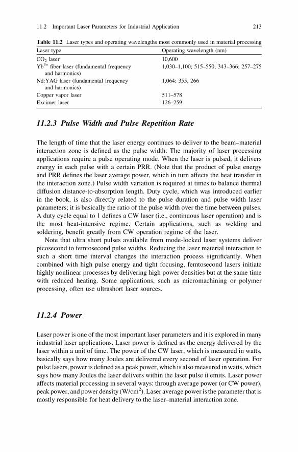
11.2.3 Pulse Width and Pulse Repetition Rate

The length of time that the laser energy continues to deliver to the beam–materialinteraction zone is defined as the pulse width. The majority of laser processingapplications require a pulse operating mode. When the laser is pulsed, it deliversenergy in each pulse with a certain PRR. (Note that the product of pulse energyand PRR defines the laser average power, which in turn affects the heat transfer inthe interaction zone.) Pulse width variation is required at times to balance thermaldiffusion distance-to-absorption length. Duty cycle, which was introduced earlierin the book, is also directly related to the pulse duration and pulse width laserparameters; it is basically the ratio of the pulse width over the time between pulses.A duty cycle equal to 1 defines a CW laser (i.e., continuous laser operation) and isthe most heat-intensive regime. Certain applications, such as welding andsoldering, benefit greatly from CW operation regime of the laser.

Note that ultra short pulses available from mode-locked laser systems deliverpicosecond to femtosecond pulse widths. Reducing the laser material interaction tosuch a short time interval changes the interaction process significantly. Whencombined with high pulse energy and tight focusing, femtosecond lasers initiatehighly nonlinear processes by delivering high power densities but at the same timewith reduced heating. Some applications, such as micromachining or polymerprocessing, often use ultrashort laser sources.

11.2.4 Power

Laser power is one of the most important laser parameters and it is explored in manyindustrial laser applications. Laser power is defined as the energy delivered by thelaser within a unit of time. The power of the CW laser, which is measured in watts,basically says how many Joules are delivered every second of laser operation. Forpulse lasers, power is defined as a peak power, which is also measured in watts, whichsays how many Joules the laser delivers within the laser pulse it emits. Laser poweraffects material processing in several ways: through average power (or CW power),peak power, and power density (W/cm2). Laser average power is the parameter that ismostly responsible for heat delivery to the laser–material interaction zone.

Table 11.2 Laser types and operating wavelengths most commonly used in material processing

Laser type Operating wavelength (nm)

CO2 laser 10,600Yb3+ fiber laser (fundamental frequency

and harmonics)1,030–1,100; 515–550; 343–366; 257–275

Nd:YAG laser (fundamental frequencyand harmonics)

1,064; 355, 266

Copper vapor laser 511–578Excimer laser 126–259

11.2 Important Laser Parameters for Industrial Application 213

11.2.5 Power Density

Power density is determined as the laser beam power over an area of the beamfocal spot in the processing zone. It basically says how many photons (and theirenergies) travel to the beam–material interaction area every second. Power densityis measured in terms of watts per centimeters squared and is calculated as pulseenergy divided by spot size. Even in a single spot, the power density can varysignificantly depending on the beam quality of the laser. Table 11.3 demonstratesseveral examples of required power densities for most important laser materialprocessing applications.

11.2.6 Laser Beam Quality

Laser beam quality is a measure of the beam quality deviation from the ‘‘ideal’’diffraction-limited Gaussian beam. At the same time, in the context of materialprocessing applications, the beam quality also implies an energy distribution in thelaser beam, which in turn affects the laser–material interaction process and theresult of material treatment. A beam, as it was discussed earlier in the book, ischaracterized using an M2 value, which is equal to 1 for a perfect Gaussian beam(i.e., its fundamental transverse mode). Most desired beam qualities for materialprocessing applications are close to those with an M2 of 1 (usually between 1 and1.5) and demonstrate a central lobe of intensity distribution close to that of aGaussian profile.

Applications such as micromachining or small-hole drilling require an M2 of*1, whereas applications such as welding and cutting may benefit from high M2

values of *50. Taking into account that most lasers with a high value of the M2

parameter have higher beam power, one may consider the beam quality togetherwith power required for the particular application (i.e., temperature rise). Note thatM2 affects the focusing capability of the beam and more accurately the beamRayleigh range, which in turn affects the depth of the focus.

As an example, UV excimer lasers, which have very poor beam quality but highpulse energy, cannot be tightly focused. However, because of the uniqueness ofthis laser type to operate in the UV spectral range with high pulse energies,excimer lasers are widely used by masking their beams to produce a desiredpattern at the interaction zone. Excimer lasers are commonly used for etching

Table 11.3 Power densityvalues for several materialprocessing applications

Material treatment process with lasers Power density (MW/cm2)

Welding *0.1Cutting 1–100Marking 10Micromachining 10–1,000

214 11 Fiber Industrial Applications of Fiber Lasers

(i.e., silicon chips) and Bragg fiber grating manufacturing, which in turn plays avery important role in fiber laser development. This spectral range (i.e.,126–259 nm) is a challenging one for fiber lasers.

11.2.7 Spot Diameter

A laser beam is usually focused onto the interaction zone. The focused laser beamsize is determined by a focal spot diameter. Focal spot diameter is a function of thefocusing lens focal length, the laser beam quality, the laser wavelength of oper-ation, and the laser beam diameter before focusing:

dspot ¼ 4FlensM2 kp � D

ð11:3Þ

where Flens is the focal length of the lens, M2 is the beam quality parameter, k isthe laser wavelength, and D is the laser beam diameter before focusing.

11.3 Fiber-Optic Power Delivery Systems

Several important applications (e.g., material processing, medicine, imaging,military) require reliable, flexible, and high-quality laser beam delivery systems.As a result, fiber-optic power delivery systems are considered to be some of themost promising solutions. At the same time, the widespread use of the fiber lasertechnology creates a potential for a unique combination of fiber lasers and fiberpower-delivery systems. Fiber-optic delivery systems demonstrate a number ofimportant advantages compared with traditional free-space solutions, including thefollowing:

1. Mechanical flexibility of the optical guide2. Separation in the space of the laser source and the workplace (the target)3. Elimination of complex and often expensive opto-mechanics4. Access to small spaces5. The possibility to affect (homogenize) an intensity profile of multimode laser

beams6. The possibility of spatial mode filtering7. Improvement of beam pointing stability (spatial jitter)8. The possibility of compact bundling of several fiber-optic sources due to a

small diameter of individual fibers9. Easy field servicing of the power transport systems (replacement and repair)

10. Reduced cost of some components

11.2 Important Laser Parameters for Industrial Application 215

There are also challenges in the fiber type of the optical power delivery system.The main challenges are:

1. Propagating power/energy limitations2. Polarization preservation of high-power guided beams3. Beam quality preservation of high-power beams

This section reviews the primary elements of fiber-optic power delivery systemsand the fiber laser output, as well as the main types of optical fiber devices used foroptical power transfer.

As was described earlier in the book, high beam–quality fiber lasers (particu-larly in commercially available systems) typically use either single-mode opticalfibers or large-mode area fibers. Both of these types of fibers allow for an optionalpolarization-maintaining feature. The typical core mode field diameters of theoptical fibers of high beam–quality fiber lasers are between 6 and 35 lm. Usingthe square root law, one may calculate the optical damage threshold for propa-gating nanosecond pulses in these fibers, which gives the damage threshold valueon the order of several J/cm2. This, in turn, gives the maximum propagating in thefiber pulse energy of a fraction of a millijoule. At the same time, the nonlinearscattering processes described earlier, such as stimulated Brillouin scattering andstimulated Raman scattering, also limit the peak power of propagating pulses toseveral tens of kilowatts. Therefore, for safe and reliable operation, optical powerdelivery systems based on optical fibers need to be carefully designed. Forapplications where sub-millijoule, nanosecond optical pulses are sufficient, onemay use a properly terminated single-fiber laser source to bring the requiredoptical power to the workplace. However, other applications may require higherpulse energies and average powers.

Examples of fiber-optic delivery systems

Several solutions have been suggested and experimentally demonstrated toincrease the damage threshold and therefore increase the power level of fiber-opticbeam delivery systems. The most adopted approaches are using fiber bundles,using photonics fibers, and using hollow fibers. This section reviews the funda-mental properties of each of these approaches.

Fiber Bundles:

As mentioned, the individual single optical fiber has a limited capacity totransmit a high-power and high-pulse energy beam. It is therefore reasonable toexpect that with a closely packed array of single fibers, one can scale the trans-mitted power practically linearly with the number of used individual fibers. This isexactly the idea behind a system called a fiber bundle. Typically, the fiber bundleconsists of an array of several multimode fibers packed together (usually glued).Each individual fiber carries light independently. Therefore, in most cases, opticaldamage and power limitation conditions have to be considered separately for eachfiber.

216 11 Fiber Industrial Applications of Fiber Lasers

(a) Manufacturing of fiber-optic bundles

The first step in manufacturing a fiber optic bundle is the creation of a singlefiber. The single fiber is manufactured/drawn from a preform (see Chap. 4 fordetails). After the single fiber is created, a number of these fibers (typicallybetween 40 and 200) are bundled together. The bundled fibers are then packedtogether, heated, and again drawn, creating a very robust array of such multifibers,which are a few millimeters in diameter. Lastly, the created multifibers (about 200)are again packed together following heating and drawing processes, which resultin a fiber bundle consisting thousands of single fibers (Fig. 11.2).

It is important to note that each individual fiber has its own cladding, which isbasically preserved during the bundle manufacturing process. During the lightinjection at the input port of the bundle, some light gets trapped in the fibercladding. The bundle design usually takes this into consideration by creating layersbetween individual fibers (which acts as an outer cladding) to dump (absorb) thecladding propagating light. Cladding propagating power limits the overall trans-mission efficiency of the fiber bundle. Typical power attenuation of the fiberbundle in the visible-infrared spectral range is in the order of a few dB/m (usuallyaround 1–1.2 dB/m). Spectrally, glass fiber bundles operate at between 400 and2,200 nm. Fiber bundles, which are used for UV applications (such as UV curingdevices), employ special UV-transmitting individual fibers; the bundle operates inthe wavelength range below 400 nm with better than 45 % optical transmission[6]. There are fiber bundles created by the utilization of plastic individual fibers.Such bundles are typically used in the visible range of optical spectrum(*400–700 nm).

Fig. 11.2 Multibundlefiber-optic structure

11.3 Fiber-Optic Power Delivery Systems 217

(b) Coherent and noncoherent fiber-optic bundles

There are a number of applications where one requires the transmission ofimages through a mechanically flexible waveguide, rather than optical power. Inthese applications, it is very important to preserve the relative position of indi-vidual fibers within the bundle at both ends of the device. Because a structuredfiber bundle preserves the original image at the output port, the fiber bundles arereferred to as ‘‘coherent bundles’’. Coherent bundles preserve spatial variation ofthe injected intensity of the optical beam at the input port of the bundle. As one canexpect, the image’s spatial resolution is basically determined by the center-to-center spacing of individual fibers in the bundle (Dd) and the transverse magni-fication of the lens system (Mlens), which couples and decouples an optical beam inand from the fiber-optic bundle [6]:

Dx ¼ Dd

Mlens

ð11:4Þ

Figure 11.3 illustrates a basic cross-sectional structure of the fiber-optic bundle.Note that an alternative way to achieve a lateral magnification in the fiber bundle isto use a tapered individual fiber.

(c) Power transmission by fiber-optic bundles

In addition to the transfer mentioned above, fiber-optic bundles are used forpower/energy delivery. Fiber bundles may also be used to divide light from asingle source into several beams or to reshape an original beam in order to coupleit between different optical devices. For energy transmission applications, theindividual fiber requirements are more lenient because the transmitted pulseenergy scales with the number of fibers in the bundle, allowing one to keep thepropagating energy fluence along the bundle below the damage threshold forindividual fibers. Exploring a particle image velocimetry application. Stephenset al. [7] demonstrated a high energy delivery of nanosecond optical pulses from afrequency-doubled Nd:YAG laser source. Using the fiber-optic bundle, the authors[7] delivered 25 mJ of 532 nm pulse energy to the target.

Δd center-to-center fiber spacing

Individual fiber core

Individual fiber cladding

fiber binder (epoxy)

Fig. 11.3 Cross sectionalstructure of a singlefiber-optic bundle

218 11 Fiber Industrial Applications of Fiber Lasers

(d) Pump combiner/coupler

Chapter 10 described so-called fused pump combiners. Such polarization-maintaining and single-mode pump combiners with feed-through double-cladfibers play a very important role in fiber laser and fiber amplifier technologies. Avariation of fiber-optic bundling technology, namely a fused modification of it,plays a very important role in combining and transferring optical power fromseveral fiber-coupled laser sources. A fused-fiber pump combiner without a feed-through fiber but with an output multimode fiber may act as an N ! 1 type ofoptical coupler/combiner (Fig. 11.4) and is widely used for direct pumpingapplications in fiber laser and fiber amplifier systems.

In several applications, such as material processing, in which it is required todeliver an average power to the target with relaxed requirements for the polari-zation and beam quality, such pump couplers are very useful. Fused-pump cou-plers/combiners deliver several hundred watts of optical power from a singleoutput fiber. The advantage of such a coupler is in a single-fiber (round) output,high pump laser-coupling efficiency ([90 %), and mechanical flexibility of thepower delivery system. Note that, as in any optical system, it is necessary toconsider brightness preservation during the design of such N ! 1 optical couplers.

Photonics Fibers:

Photonics crystal fibers (PCF) (Holley fibers), which appeared in the early1990s, have a special place in the fiber science and technology. Due to their uniqueproperties (mainly versatility), they are widely used and have become uniqueplayers in several important applications, ranging from fiber laser sources tooptical power guides.

Following Tünnermann et al. [8], we will review the main technical charac-teristics of this type of optical fiber. Figure 11.5a shows a fundamental cross-sectional view of the PCF. The basic idea behind PCF technology is to achieve acontrollable refractive index profile in the fiber cladding by creating an array of airholes in the fiber cladding. The air holes have diameter d and pitch K. The holes’orientation follows a triangular geometry, as shown in Fig. 11.5a, b.

Fusion area

Single outputMM fiber

Example: 105/125 NA=0.22

Input MM fibersExample: 105/125 NA=0.15

INPUT

OUTPUT

Fig. 11.4 Fused opticalpump-coupler structure.Numerical aperture (NA)

11.3 Fiber-Optic Power Delivery Systems 219

As one can expect, filling the fiber cladding with multiple air holes reduces anaverage (or effective) refractive index of the cladding glass. This in turn shouldaffect both the propagating condition of the optical waves inside the fiber core(condition of the total internal reflection) as well as the numerical aperture (NA) ofthe fiber core.

The V-parameter of the PCF can be expressed as follows [9]:

VPCFðkÞ ¼2pk

Kffiffiffiffiffiffiffiffiffiffiffiffiffiffiffiffiffiffiffiffiffiffiffiffiffiffiffiffiffiffiffiffiffiffiffi

nðkÞ2core � nðkÞ2clad

q

ð11:5Þ

For VPCF [ p, the fiber starts supporting high-order propagating modes (cutoffcondition) [9]. Unlike conventional step-index fibers, where wavelength depen-dence of the refractive index of the cladding material follows the conventionaldispersion trend, the effective refractive index of the PCF has a very strongwavelength dependence (Fig. 11.6).

As shown in Fig. 11.6, for a very big pitch value K compared with the wholediameter d (more glass mass in the cladding structure), the effective refractiveindex basically approaches the refractive index of the solid glass. In the oppositecase—that is, when the value of the pitch is close to that of the air hole diameter—the effective refractive index decreases (more air in the cladding structure). Whenaddressing the condition of single-mode propagation in PCF, it is useful to illus-trate a plot, as shown in Fig. 11.7.

PCF GlassCore

Air

Glass

(a)

(b)

Fig. 11.5 a Fundamental,cross-sectional structure of aPCF. b Scanning electronmicroscope micrographs of aPCF produced by the NavalResearch laboratory (left).The diameter of the solid coreat the center of the fiber is5 lm, whereas the diameterof the holes is 4 lm (right).(Reproduced from US NavalResearch Laboratory at http://www.nrl.navy.mil/techtransfer/viewpdf_st.php?id=70)

220 11 Fiber Industrial Applications of Fiber Lasers

Figure 11.7 demonstrates a dependence of the wavelength to the pitch ratio k=Kversus the relative hole diameter d=K. As one can see from Fig. 11.7, when therelative air hole diameter is less than 0.45, the PCF demonstrates a single spatialmode propagation for any wavelength (endlessly single-mode PCF) [10]. Animportant conclusion can be made when PCF demonstrates a relative hole diam-eter less than 0.45. In this case, one may achieve a single mode propagation withtheoretically any core size, provided that the pitch value is chosen accordingly.Note, however, that if the value k=K becomes too small (\0.1), scattering loss dueto longitudinal nonuniformities such as microbending, macrobending, anddielectric imperfections increases [11].

Preserving a single spatial propagating mode in a wide range of the fiber coresizes is a very useful property of the PCF for high-energy and high-power fiberlaser and optical power transfer applications, for which achieving a high energy ofa single transverse mode propagation in a conventional rare-earth-doped glass fiber

Fig. 11.6 Effective index ofrefraction of a photonicscrystal fiber cladding. (Imagecourtesy of Springer)

Fig. 11.7 Single-modeversus multimode conditionsin photonics crystal fiber.(Image courtesy of Springer)

11.3 Fiber-Optic Power Delivery Systems 221

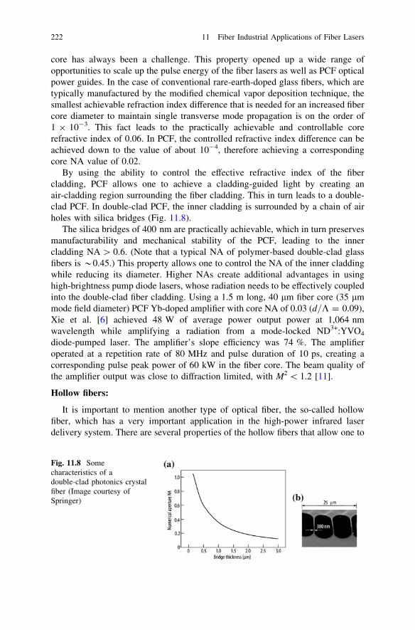
core has always been a challenge. This property opened up a wide range ofopportunities to scale up the pulse energy of the fiber lasers as well as PCF opticalpower guides. In the case of conventional rare-earth-doped glass fibers, which aretypically manufactured by the modified chemical vapor deposition technique, thesmallest achievable refraction index difference that is needed for an increased fibercore diameter to maintain single transverse mode propagation is on the order of1 9 10-3. This fact leads to the practically achievable and controllable corerefractive index of 0.06. In PCF, the controlled refractive index difference can beachieved down to the value of about 10-4, therefore achieving a correspondingcore NA value of 0.02.

By using the ability to control the effective refractive index of the fibercladding, PCF allows one to achieve a cladding-guided light by creating anair-cladding region surrounding the fiber cladding. This in turn leads to a double-clad PCF. In double-clad PCF, the inner cladding is surrounded by a chain of airholes with silica bridges (Fig. 11.8).

The silica bridges of 400 nm are practically achievable, which in turn preservesmanufacturability and mechanical stability of the PCF, leading to the innercladding NA [ 0.6. (Note that a typical NA of polymer-based double-clad glassfibers is *0.45.) This property allows one to control the NA of the inner claddingwhile reducing its diameter. Higher NAs create additional advantages in usinghigh-brightness pump diode lasers, whose radiation needs to be effectively coupledinto the double-clad fiber cladding. Using a 1.5 m long, 40 lm fiber core (35 lmmode field diameter) PCF Yb-doped amplifier with core NA of 0.03 (d=K = 0.09),Xie et al. [6] achieved 48 W of average power output power at 1,064 nmwavelength while amplifying a radiation from a mode-locked ND3+:YVO4

diode-pumped laser. The amplifier’s slope efficiency was 74 %. The amplifieroperated at a repetition rate of 80 MHz and pulse duration of 10 ps, creating acorresponding pulse peak power of 60 kW in the fiber core. The beam quality ofthe amplifier output was close to diffraction limited, with M2 \ 1.2 [11].

Hollow fibers:

It is important to mention another type of optical fiber, the so-called hollowfiber, which has a very important application in the high-power infrared laserdelivery system. There are several properties of the hollow fibers that allow one to

Fig. 11.8 Somecharacteristics of adouble-clad photonics crystalfiber (Image courtesy ofSpringer)

222 11 Fiber Industrial Applications of Fiber Lasers

transmit and deliver optical power where and when traditional solid-core opticalfibers show limited performance:

1. The spectral transmittance of hollow fiber is beyond the 20 lm wavelengthrange.

2. Hollow fiber has a relatively simple structure, which makes this system man-ufacturable and cost effective.

3. Hollow fiber has an air core, which significantly increases the optical damagethreshold (important for high-power applications).

Historically, hollow fibers have been developed and used for optical powerdelivery of high-power CO2 lasers operating at the 10.6 lm wavelength. High-power CO2 lasers are still widely used in laser material processing and occupy abig fraction of the laser market. When properly designed, hollow fibers demon-strate low insertion loss (*0.1–1 B/m). Note that the high loss nature of hollowfibers compared with all glass telecommunication fibers, where insertion losses areon the order of *0.2 dB/km, is one of the biggest limiting factors in the wide-spread use of hollow fibers.

Naturally hollow fibers show no Fresnel reflection at the input and output portsof the waveguide and, because of the air-fill core, the hollow fibers demonstratelow divergence of the output beam (low NA). Mechanically, hollow fibers aregenerally less flexible (bending strength). Nevertheless, an ability to transmit high-infrared optical power (several kilowatts) [12] makes them irreplaceable in severalapplications, ranging from laser material processing to laser surgery.

There are two main types of hollow waveguides [13]:

1. ‘‘Leaky guides’’, with an inner core refractive index of n [ 1.2. Attenuated total reflectance (ATR) guides, with an inner wall material with a

refractive index of n \ 1.

The two main structures of the hollow waveguides are shown in Fig. 11.9.The leaky guide, with n [ 1, employs a metallic and dielectric film deposited

on the inside of metallic, plastic, or glass tubing. The ATR type, which has innerwall material with n \ 1, is composed of dielectric materials and acts as a fiber

AirStructural tube

Dielectric Coating

Metallic film

Airn<1

material

(a) (b)Fig. 11.9 Two types ofhollow waveguides. a Leakyguide. b Attenuated totalreflectance guide

11.3 Fiber-Optic Power Delivery Systems 223

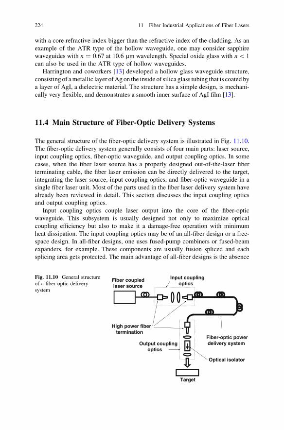
with a core refractive index bigger than the refractive index of the cladding. As anexample of the ATR type of the hollow waveguide, one may consider sapphirewaveguides with n = 0.67 at 10.6 lm wavelength. Special oxide glass with n \ 1can also be used in the ATR type of hollow waveguides.

Harrington and coworkers [13] developed a hollow glass waveguide structure,consisting of a metallic layer of Ag on the inside of silica glass tubing that is coated bya layer of AgI, a dielectric material. The structure has a simple design, is mechani-cally very flexible, and demonstrates a smooth inner surface of AgI film [13].

11.4 Main Structure of Fiber-Optic Delivery Systems

The general structure of the fiber-optic delivery system is illustrated in Fig. 11.10.The fiber-optic delivery system generally consists of four main parts: laser source,input coupling optics, fiber-optic waveguide, and output coupling optics. In somecases, when the fiber laser source has a properly designed out-of-the-laser fiberterminating cable, the fiber laser emission can be directly delivered to the target,integrating the laser source, input coupling optics, and fiber-optic waveguide in asingle fiber laser unit. Most of the parts used in the fiber laser delivery system havealready been reviewed in detail. This section discusses the input coupling opticsand output coupling optics.

Input coupling optics couple laser output into the core of the fiber-opticwaveguide. This subsystem is usually designed not only to maximize opticalcoupling efficiency but also to make it a damage-free operation with minimumheat dissipation. The input coupling optics may be of an all-fiber design or a free-space design. In all-fiber designs, one uses fused-pump combiners or fused-beamexpanders, for example. These components are usually fusion spliced and eachsplicing area gets protected. The main advantage of all-fiber designs is the absence

Fiber coupled laser source

High power fibertermination

Fiber-optic power delivery system

Input coupling optics

Output coupling optics

Target

Optical isolator

Fig. 11.10 General structureof a fiber-optic deliverysystem

224 11 Fiber Industrial Applications of Fiber Lasers

of free-space zones with high-power beams, mechanical flexibility, and no need forpreserving precise alignment of each component during the operation. The maindisadvantage is mostly in servicing, for which one needs to use an expensivefusion splicer and, in some cases, optical power limitation of available individualfiber components.

A free-space input optical coupling design offers the greatest flexibility in opticaldesign, flexibility in available free-space components, and the ability to use afree-space laser output beam, which in some cases may have advantages over fiber-coupled lasers. In the case of the free-space input optical coupler design, it is veryimportant to collect most of the laser power into the haul fiber core while taking intoaccount the fiber NA (acceptance angle of the fiber). Any light coupled into the fibercladding produces the system loss (decreased coupling efficiency) and increaseslocal temperatures, which in turn may lead to a catastrophic failure of the couplingoptics and even the fiber-optic waveguide. In the free-space input coupling opticsdesign, each fiber entrance requires proper termination. High-power fiber termi-nations are commercially available from several vendors. The fiber terminationsusually use AR coating as well as angle-polished fiber ends enclosed in high-powerfiber sockets. Note that it is extremely important to keep all optical interfaces cleanof dust and other contaminations that cause high-power laser beam scattering,burns, and as a sequence, optical damage of the glass surfaces.

Output coupling optics couple out laser beam propagating in the opticalwaveguide and focus the laser beam on a target for laser processing of the material.It is often important to incorporate a high-power optical isolator into the outputcoupling optical system because of the danger of back reflection for fiber laseroperations. The output coupling optics may include high-power fiber termination,a beam expander, and a beam focusing assembly. The particular design is dictatedmostly by the application, which may require a different focal spot, depth offocusing, and beam position precision.

11.5 Main Industrial Applications of Fiber Lasers

11.5.1 Welding

Welding is one of the most widely used applications in laser material processingand is directly related to high-power laser beams. This process requires delivery ofcertain laser power to the interaction zone within a certain period of time, which inturn is converted to the heat required for the welding process. Deposited heat thensoftens the material leading to the welding. Because of the well-controlled outputpower and heating time through laser pulse duration, lasers are considered bymany to be an ideal welding tool. Among the advantages that are demonstrated bycurrent state-of-the art current laser welding processes, one may mention precisionof welding parameters, high power density, a small interaction zone (which in turn

11.4 Main Structure of Fiber-Optic Delivery Systems 225

comes from the capability to deliver high power into a small spot), low distortionof the affected welding area, high speed of the process, and the possibility of laserwelding in air.

Disadvantages of laser welding usually come from the cost of laser weldingequipment, including high-power lasers (although fiber laser is expected to reducethe cost of ownership), requirements of well-aligned joints of the samples, as wellas dealing with high metal reflectivity of the infrared light used from high-powerlasers. Temporal regimes required for laser welding span from millisecond to CWlaser operations. Lasers with more than 1 kW of average power are usuallyrequired for both welding and cutting.

11.5.2 Cutting

Laser cutting is a process that uses a focused laser beam as a heat source to melt andthen to vaporize sample material, which in turn during sample (or beam) movingleads to the sample partition. Laser cutting is usually optimized by varying laserpower, sample feeding, and power density. Similar to welding, laser cutting usuallyuses high-power lasers and is considered a fast process when optimized. Lasercutting typically uses microsecond, millisecond, or CW laser operating regimes.

11.5.3 Drilling

During the laser drilling process, the sample material is removed to create via holes.Drilling is usually accomplished by so-called percussion or trepanning drillingprocesses. The percussion drilling process sets the focal spot diameter close to thetargeted hole size. However, there are situations (especially when the laser power islimited) when large holes have to be drilled. In this case, trepanning drilling is asolution. In this technique, the laser focal spot size is set to be smaller than thetargeted hole and the laser beam is moved within the targeted hole dimension to‘‘free’’ the area and create the hole of desired diameter. Laser drilling uses micro-second, nanosecond, and picosecond laser pulses. It is considered to be cost-effective because there is no drill breakage or wear and it is highly reproducible.

11.5.4 Soldering

Soldering uses high-power laser beams and requires local heating of samples.Fiber lasers with controlled pulse widths and controlled high average powerproduce a fast soldering process. Soldering uses millisecond to CW laser operatingregimes when high average powers are achieved.

226 11 Fiber Industrial Applications of Fiber Lasers

11.5.5 Marking

Laser marking uses a so-called ‘‘thermal shock’’ or a fast heat dissipation toremove a sample material surface layer. Laser marking has an important role inlaser material processing and generates good revenues for material processingcompanies. Because they are flexible in wavelength selection as well as temporaland energy parameters, lasers are becoming one of the most popular marking toolsfor many surfaces, including metal and plastic materials. Unlike other markingtechniques, such as printing, laser marking is a clean process that does not usehazardous materials, has a low cost of ownership, and is highly flexible for dif-ferent marking requirements. Laser marking is very stable. Laser marking typicallyuses nanosecond pulse operating regimes with \100 W of average powers. Fiberlasers are an ideal solution for laser marking applications.

11.5.6 Heat Treating

Because of their high power and tight focusing capabilities, lasers are widely usedin material local heating. Some applications require stress removal from thelocalized area without spreading the heat to the whole workpiece. Laser heatinguses localized material treatment and minimizes material distortion and stress.Laser heating uses millisecond to CW laser operation, often with good beamquality, especially when hard-to-access areas have to be heated.

11.5.7 Metal Deposition

Laser metal deposition is the process during which some metal parts are built byinjecting metal powders into the focused spot of a high-power CW laser beam. Themetal parts created as a result of direct metal deposition vary in mechanicalproperties depending on the metal alloys used during the process. Metal depositionusing high-power CW lasers is a fast process of manufacturing different parts ortheir repair.

11.5.8 Paint Stripping and Surface Removal

During laser paint stripping, painting material is removed from the sample surface.Basically, because there is no contact operation, lasers offer a clean and safesurface treatment environment with a precisely defined depth of laser–materialinteraction. (This is unlike chemical stripping, in which special care should be

11.5 Main Industrial Applications of Fiber Lasers 227

taken for the waste disposal as well as the non–localized effects of chemicals,which may spread to the other material parts and even removing unintended part ofthe sample material.) Stripping is implemented though material removal viavaporization of the painted material without significant color change or othersample degradation. Basic requirements for the surface removal or paint strippingare high absorbance of the paint at the laser wavelength and low thermalconductivity.

11.5.9 Micromachining

Micromachining is probably the most precise type of laser material processing.The process results in the production of very small parts. The process requires heatdissipation in a very small area during a very small period of time. Microma-chining requires high peak power and very short pulses, but low average power.The speed of the laser should be in the multi-kilohertz range of PRR with pico-second to femtosecond pulse durations. With shorter wavelengths and better beamquality, the process resolution increases. Micromachining is applied to metals,plastics, and composites, among others. The micromachining process using veryhigh peak power femtosecond lasers employs ionization of the material, whichtakes place in the high-intensity field of the laser beam. Micromachining requiresmode-locked lasers, which are costly compared with long-pulse and CW models.However, the advantages achieved by using a femtosecond pulse justify its use inmost micromachining applications.

11.5.10 Semiconductor Processing with a Laser Beam

Laser processing of semiconductor materials plays an important role in today’slaser applications. Semiconductors generally have strong absorption in the UV,visible, and near infrared region while demonstrating high transparency in theinfrared region of the optical spectrum. The 1,064 nm fiber and DPSS lasers areused mostly for silicon marking, whereas UV lasers (e.g., excimer) or harmonicsof fiber lasers are used for material processing of wide-bandgap semiconductors,such as gallium arsenide and indium phosphide. The temperature of the semi-conductor sample is used as an optimization parameter during processing becauseof its effect on the light absorption.

Figure 11.11 shows most of the laser material processing applications on a mapof beam quality and required laser operating average powers. As one can see, fiberlaser sources that demonstrate 3–5 kW power with diffraction-limited beamquality and up to 50 kW in multitransverse mode operation meet most ofrequirements and are a good fit for numerous applications.

228 11 Fiber Industrial Applications of Fiber Lasers

11.5.11 Main Competitors of Fiber Lasers in IndustrialLaser Applications

This section reviews the main competitors of fiber lasers used in material pro-cessing applications. Besides fiber lasers, the most widely used laser types includediode lasers, DPSS (Nd:YAG, Yb3+:YAG, Nd:VO4), solid-state thin-disk lasers,CO2 (high cost of ownership), and excimer lasers.

Although fiber laser technology is quickly replacing many diode lasers andDPSS lasers in rod and slab configurations, it still competes with solid-state thin-disk lasers that have appeared during the last decade. Thin-disk lasers have severalunique properties and therefore are considered to be one of the main competitorsfor fiber laser technology in current solid-state laser material processing. Espe-cially in applications requiring high average powers, thin-disk lasers remain indemand, even though industrial fiber lasers have demonstrated multi-kilowattlevels of operation.

Thin-disk lasers have a power-scalable (with the disk area) platform withreasonably good beam quality. Disk lasers provide short (nanosecond) pulses witha high peak power of operation. Currently, disk lasers are superior to fiber lasers inhigh-energy nanosecond pulses. Disk lasers are very attractive for weldingapplications in which high beam quality is required along with multi-kilowattoutput powers. Disk lasers are not susceptible to back reflection from highlyreflecting metal surfaces. They also are more tolerant to high-power and high-energy scaling because their intracavity light fluence is far from the optical

Fig. 11.11 Laser beam quality and average power map for different material processingapplications [11, 14] (Image courtesy of SPIE)

11.5 Main Industrial Applications of Fiber Lasers 229

damage threshold, which in turn make them quite reliable in some sensitive(failure intolerant) applications.

The long-existing gas CO2 lasers also occupy a significant part of the lasermaterial processing market because of their high power availability, especially forapplications such as welding and cutting. Using unstable laser resonators, CO2

lasers may provide diffraction-limited beam quality at elevated optical powers.Some applications that require laser wavelengths in the infrared range benefit fromthe 10 lm line of this laser. Note, however, that probably the most seriousadvantage of the CO2 laser is that they are already installed in many materialprocessing centers and companies. Even if all other parameters of fiber lasersincluding power, beam quality, and wavelength will satisfy the user, CO2 laserswill still remain on the market. There is also a discussion currently about theadvantages of using CO2 lasers versus fiber lasers in metal welding and cutting.

Excimer lasers emitting in the 126–259 nm spectral range, with their high pulseenergy reaching several hundreds of millijoules and relatively high PRR current,remain out of touch for many applications, such as lithography. Most high-powerfiber lasers operate in the near-infrared spectral range and require nonlinear fre-quency conversion to reach UV wavelengths of operation. This in turn requireshigh energy and high peak powers. Their small core size (on the order of 30 lmfor diffraction-limited systems and several hundreds of micrometers for multimodeoperation) significantly restricts the fiber laser’s pulse energy in the nanosecondrange of pulse durations. Excimer lasers will probably remain out of competitionfrom fiber lasers for most lithography applications in the near future.

11.5.12 Summary of Challenges for Fiber Lasersin Industrial Applications

In summary, the challenges facing fiber lasers in industrial applications include thefollowing:

• Back reflection when processing highly reflective materials, such as those withmetal-coated surfaces or metal parts.

• Pulse energy scaling for nanosecond fiber lasers systems due to fiber materialsurface and bulk damage.

• Availability of infrared wavelengths in the vicinity of CO2 laser sources (i.e., inthe 10 lm spectral range) for immediate and painless substitution of gas lasersources.

• Availability of visible (especially blue) and UV wavelengths with power-scalable concepts, which can effectively compete with blue-green solid state andexcimer lasers.

• Reliable and high value of polarization extinction ratio at elevated power levelswith diffraction beam quality (when nonlinear frequency conversion isconsidered).

230 11 Fiber Industrial Applications of Fiber Lasers

11.5.13 Future of Fiber Lasers in Material Processing

High-power fiber lasers will continue to penetrate the laser material processingmarket, especially where flexibility in pulse profiles, PRR, and power density arerequired. The biggest challenge will probably be in penetrating those marketswhere laser applications require more than 100 mJ of nanosecond pulses in boththe UV and infrared spectral range. Even though today the total industrial fiberlaser market totals several hundred million dollars and the whole laser materialprocessing market totals a few billion dollars, fiber lasers show great potential andpromise. Fiber lasers are already widely used for marking, thin-film ablation,welding, cutting, and semiconductor material processing (e.g., silicon). The uniqueand flexible fiber laser systems with low cost of ownership and all-fiber archi-tecture definitely make fiber laser technology a top choice for numerous materialprocessing applications.

References

1. W.M. Steen, K. Watkins, Laser Material Processing, 3rd edn. (Springer Verlag LondonLimited, UK, 2003), p. 401

2. R. Iffländer, Solid-State Lasers for Materials Processing (Springer Verlag Berlin, 2001), p. 3473. J.F. Ready, Industrial Applications of Lasers (Academic Press, New York City, 1997)4. J.P. Holman, Heat Transfer, 9th edn. (McGraw-Hill, New York, 2002) (which in turn cites A.I.

Brown, S.M. Marco, Introduction to Heat Transfer, 3rd edn., McGraw-Hill, New York, 1958and E.R.G. Eckert, R.M. Drake, Heat and Mass Transfer, McGraw-Hill, New York, 1959)

5. A. Bejan, J. H. Boyett, A.D. Kraus, Heat Transfer Handbook (Wiley-IEEE, NJ, 2003), p. 14966. T. Xie, D. Mukai, S. Guo, M. Brenner, Z. Chen, Fiber-optic-bundle-based optical coherence

tomography. Opt. Lett. 30, 1803–1805 (2005)7. T.J. Stephens, M.J. Haste, D.P. Towers, M.J. Thomson, M.R. Taghizadeh, J.D.C. Jones, D.P.

Hand, Fiber-optic delivery of high-peak-power q-switched laser pulses for in-cylinder flowmeasurement. Appl. Opt. 42, 4307–4314 (2003)

8. A. Tünnermann, J. Limpert, A. Bruns, in Diode-Pumped Fiber Lasers. Chapter 4.3 in LaserSystems, Part 2, Landolt-Börnstein—Group VIII Advanced Materials and Technologies, vol.12 (Springer, 2008), pp. 125–139

9. N.A. Mortensen, J.R. Folkenberg, M.D. Nielsen, K.P. Hansen, Modal cutoff and theV parameter in photonic crystal fibers. Opt. Lett. 28, 1879–1881 (2003)

10. T.A. Birks, J.C. Knight, P.S.J. Russell, Endlessly single-mode photonic crystal fiber. Opt.Lett. 22, 961–963 (1997)

11. J. Limpert, A. Liem, M. Reich, T. Schreiber, S. Nolte, H. Zellmer, A. Tünnermann,J. Broeng, A. Petersson, C. Jakobsen, Low-nonlinearity single-transverse-mode ytterbium-doped photonic crystal fiber amplifier. Opt. Express 12, 1313–1319 (2004)

12. A. Hongo, K. Morosawa, K. Matsumoto, T. Shiota, T. Hashimoto, Transmission of kilowatt-class CO2 laser light through dielectric-coated metallic hollow waveguides for materialprocessing. Appl. Opt. 31, 5114–5120 (1992)

13. J.A. Harrington, A review of IR transmitting, hollow waveguides. Fiber Integr. Opt. 19,211–217 (2000)

14. W.F. Krupke, Advanced Diode-Pumped Solid-State Lasers (DPSS): Near Term Trends andFuture Prospects, in Proceedings of SPIE, 2000, vol. 3889, pp. 21–32

11.5 Main Industrial Applications of Fiber Lasers 231

Chapter 12Conclusion

This chapter outlines the major conclusions of the topics reviewed in this book.

1. The physics of fiber lasers and fiber amplifiers are the same as for any otherlaser type and follow similar theoretical considerations. Most solid-state laserformulas can be used during fiber laser design and development.

2. Unlike bulk lasers, fiber laser resonator modes of optical fibers followcylindrical geometry waveguide modes. Fundamental mode (LP01) selectiontechniques in fiber lasers and fiber amplifiers are different from that of openoptical resonators.

3. Due to long length and small cross-sectional area of the fiber-active medium,fiber laser gain is enormously high. This has two big impacts on the fiber laserposition among other laser systems:

(a) Pump-to-lasing efficiency is up to 80 %, which in turn results in a highwall plug efficiency.

(b) Because of the same long gain medium and small fiber-core cross-sectionalarea, optical nonlinearities and optical damage are serious limitations inscaling up fiber laser powers and essentially peak powers.

4. Special attention has to be paid to nonlinearities and damage issues duringfiber laser design.

5. Back-propagating signal powers inside a fiber laser system can be a realdanger for several components of the fiber laser or fiber amplifier system.Careful optical isolation of each gain stage of the system is a must for safeoperation.

6. Unlike many other laser types, fiber laser and fiber amplifier systems can bemade alignment-free due to highly developed fiber-splicing technology andavailability of fiber-coupled optical components as well as fused all-fibercomponents.

V. Ter-Mikirtychev, Fundamentals of Fiber Lasers and Fiber Amplifiers,Springer Series in Optical Sciences 181, DOI: 10.1007/978-3-319-02338-0_12,� Springer International Publishing Switzerland 2014

233

7. In the case of high average power (or high CW power), the ‘‘thermalimmunity’’ of fiber lasers would be an incorrect assumption during a fiber laserdesign process. Thermal management has to be considered for reliable oper-ation with preserved laser parameters.

8. The commercial availability of reliable and low-cost fiber-coupled opticalcomponents, including pump laser diodes for fiber lasers and amplifiers, arereal challenges. Without resolving these issues, the successful development ofthe fiber laser and fiber amplifier systems (especially high power) will be veryproblematic.

234 12 Conclusion

Index

AAbsorption, 3, 7–9, 11–13, 17–25, 30, 31, 33,

34, 37, 44, 46–47, 50, 51, 53–60, 81,86, 88, 91, 93, 95, 96, 104, 127, 134,163–165, 167, 172, 179, 197, 210–213,228

Absorption band, 3, 23, 24, 46, 47, 50, 51, 53,56, 57, 59, 167

Absorption characteristics, 172Absorption coefficient, 21, 23, 24, 35, 164,

165, 172, 212Absorption cross section, 17, 20, 22, 87, 104Absorption depth, 211Absorption frequency, 8Absorption intensity, 23Absorption length, 211, 213Absorption line, 30, 53Absorption loss, 87, 88Absorption peak, 50Absorption process, 7, 8, 12, 211, 212Absorption saturation, 87, 95Absorption spectrum, 46, 48, 51, 53, 58, 59Absorption transition, 47, 87Acoustic, 10, 174, 177, 178Acoustic branch, 10Acoustic phonon, 174, 177, 178Acoustic phonon energy, 177Acoustic velocity, 177Acoustic vibration, 177Acoustic wave, 10, 174, 177, 178Active, 1–3, 7, 9, 16, 17, 21, 23–25, 27–29, 32,

34, 37–39, 41, 44, 46, 50, 56, 58, 61,73, 80, 82, 84, 85, 87, 88, 90, 93, 94,97, 99–101, 103, 104, 106, 110, 114,115, 117, 126, 127, 129, 138, 142, 143,148, 161, 174, 175, 178, 186, 200, 209,233

Active acoustic phonon, 178Active and passive techniques, 117Active centers, 23, 56, 61, 82, 84, 104Active compensation, 200Active concentration, 16, 34, 38, 56, 88, 104,

127Active electronic transition, 9Active elements, 186Active fiber, 29, 39, 41Active glass, 30, 50, 115Active ion, 2, 3, 7, 16, 17, 21, 24, 32, 34,

37–40, 50, 56, 87, 94, 99, 104, 106,127, 161

Active laser medium, 85, 100, 110, 114, 127Active layer, 144Active level, 28Active material, 175Active media, 46, 73, 80, 99, 115Active medium, 46, 85, 88, 90, 93, 94, 97, 100,

101, 110, 114, 127, 129Active mode-locking, 117Active modulation, 101, 110, 157Active optical center, 21, 23Active phonon, 27Active Q-switching, 126Active rare-earth, 23, 40Active region, 138, 142, 143Active transition, 7, 9, 58Actively phase-locked, 200Adiabatic, 151Adiabatically, 151Adiabaticity, 151Adiabaticity criteria, 151Air core, 223Air holes, 219, 220Air/solid structure, 73Air-cladding, 222

V. Ter-Mikirtychev, Fundamentals of Fiber Lasers and Fiber Amplifiers,Springer Series in Optical Sciences 181, DOI: 10.1007/978-3-319-02338-0,� Springer International Publishing Switzerland 2014

235

Air-fill, 223Aluminum (Al), 33, 37, 38, 40, 119, 211Amplification, 1, 37, 79, 80, 82–84, 87, 89,

108, 111, 135, 141, 170, 175, 187, 190,210

Amplification and oscillation, 37, 79, 135Amplification and pulse, 89, 109, 170, 210Amplification and signal wave, 175Amplification and spontaneous emission, 84Amplification in double clad fiber, 108Amplification in fiber amplifier, 210Amplification of electromagnetic waves, 80Amplification of light, 135Amplification principle, 82Amplification process, 83Amplification stages, 89Amplified spontaneous emission (ASE), 84,

85, 105, 108, 144Amplifier, 191Amplifier and Yb3þ, 191Amplifier and Er3þ, 193Amplifier and ‘‘chopped’’ seed, 89Amplifier and Brillouin, 82Amplifier and DC fiber, 191Amplifier and fiber, 1, 4, 33, 41, 52, 53, 71,

82–89, 92, 108, 142, 148–150, 153,164, 166, 169, 171, 172, 186, 187, 190,191, 193, 194, 202, 203, 210, 219, 233,234

Amplifier and gain, 83–85, 87, 88, 190Amplifier and ideal, 85Amplifier and large-mode-area, 170Amplifier and laser, 23, 82, 83, 85, 88, 89, 151,

187Amplifier and length, 49, 85, 88, 171, 190Amplifier and level, 85Amplifier and MOPA, 108, 187, 189–191, 193,

202, 209, 210Amplifier and optical, 83, 83, 85, 86, 89Amplifier and parametric, 82Amplifier and power, 108, 130, 187, 190–193,

209Amplifier and pre-amplifier, 191–193Amplifier and pulse, 82Amplifier and pulse propagation, 89, 157Amplifier and Raman, 4Amplifier and seeded, 82, 89, 193Amplifier and solid-state laser, 88Amplifier and square pulse seeded, 89Amplifier and type, 88Amplifier application, 147Amplifier array, 187, 207Amplifier chain, 194

Amplifier configuration, 130Amplifier design, 166, 190Amplifier energy level, 192Amplifier FWHM gain bandwidth, 83Amplifier gain, 83–85, 87, 88, 190Amplifier gain coefficient, 83–85, 187, 190Amplifier gain spectrum, 85Amplifier gain volume, 88Amplifier geometry, 186, 187Amplifier inversion, 85Amplifier loss, 84Amplifier material, 83, 86, 89Amplifier noise, 85, 190Amplifier of electromagnetic oscillations, 79Amplifier output, 202, 222Amplifier phase, 85, 86Amplifier phase shift, 85, 86Amplifier power, 84Amplifier pulsing, 86Amplifier slope efficiency, 222Amplifier system, 1, 5, 85, 86, 89, 108, 169,

172, 193, 233, 234Amplifier technologies, 219Analyzer, 152, 153, 201Angle alignment, 73Angle dependence, 199Angle deviation, 199Angle of diffraction, 120, 185Angle of divergence, 73, 76, 195, 196Angle of incidence, 120Angle of tapering, 151Angle of TIR, 65Angle of total internal reflection, 185Angle polished, 225Angle selectivity, 198Anomalous, 129Anomalous behavior, 129Anomalous single frequency, 129Anti-stokes, 174, 175APCAPC connectorAPC polishAperture, 66, 84, 102, 147, 149, 151, 161, 196,

220Aperture and beam, 196Aperture and numerical, 219, 220ASE and fighting, 85ASE and measurable, 188ASE and output, 84ASE and propagating, 84, 85ASE and spontaneous emission, 84, 85, 128ASE and suppression, 193ASE filter, 194

236 Index

ASE free operation, 105, 187ASE level, 108ASE light, 84ASE noise, 84ASE photons, 84ASE power, 84, 190ASE power level, 190ASE process, 85, 144ASE source, 84Askarian, 185Astigmatic, 144, 146Astigmatic nature, 146Asymptotic, 105Asymptotic value, 105Atomic, 7, 10, 12, 79, 83, 86Atomic chain, 10Atomic decay, 11Atomic distance, 7, 10Atomic energy, 12Atomic energy level, 12Atomic line, 83Atomic line shape, 83Atomic mass, 83Atomic masses, 10Atomic nuclei, 7Atomic response, 86Atomic states, 80Atomic structure, 29Atomic system, 79Atomic transition, 83, 86ATR guides, 223ATR type, 223, 224Attenuation profile, 31Available, 4, 5, 24, 29, 32, 41, 47, 52, 82, 102,

107, 133, 144, 150, 166, 175, 209, 216,225

Available and commercially, 33, 52, 102, 107,133, 139, 144, 147, 161, 209, 216, 225

Available CCD, 76Available components, 5Available fiber, 161, 209Available laser diode, 24, 47Available phonons, 28Available solution, 4Axial, 124, 126Axial mode, 124, 126Axial mode filter, 126

BBackscattering, 178Bandgap, 133, 135, 136, 138, 142, 228

Bandwidth, 23, 59, 68, 83, 110–112 , 114,115, 123, 125, 126, 128, 157, 158,176, 179, 205

Bandwidth and chirp, 158Bandwidth and estimated, 123Bandwidth and gain, 112Bandwidth and spectral, 68, 83, 111, 126,

128, 157, 176, 179, 205Bandwidth and time bandwidth product, 115Bandwidth limited, 110Bandwidth product, 111, 115Beam, 3, 4, 56, 66, 73–77, 82, 88, 91, 102,

107, 109, 119–121, 124, 125, 127,135, 138, 142, 144, 147–149, 151,153, 155, 161, 162, 164, 165, 167,169, 171, 175, 176, 180, 182, 183,185–189, 191–198, 200–205

Beam and amplified, 88, 175, 202Beam and amplifying, 82, 88Beam and arbitrary, 74–76Beam and astigmatic, 144Beam and coherent, 162, 195, 196, 200–202,

205Beam and collimated, 121, 203Beam and co-propagation, 182Beam and diffracted, 120, 198Beam and diffraction limited, 4, 75, 102, 109,

161, 164, 188, 193, 210, 228, 230Beam and electron, 135, 138Beam and extraordinary, 153, 156Beam and focal spot, 77, 214Beam and Gaussian, 73–77, 214Beam and gravity, 73, 74Beam and guided, 216Beam and incident, 198Beam and individual, 205Beam and intra-cavity beam combination, 201Beam and laser, 73–75, 77, 82, 91, 107,

109, 119, 121, 127, 142, 147–149,175, 187, 189, 195, 202, 203, 210–212,214, 215, 225–229

Beam and light, 155, 180, 185Beam and mirror-beam combination, 200Beam and multiple, 182Beam and non-gaussian, 74Beam and optical, 82, 180, 218Beam and original, 196, 205, 218Beam and output, 121, 147, 192, 196, 202,

205, 210, 223, 225Beam and polarized, 124, 188, 195Beam and pumping, 138Beam and rayleigh range, 76, 77, 214

Index 237

Beam and real, 74Beam and reference, 203Beam and resultant, 196, 203, 205Beam and spectral beam combination, 203Beam and structure, 144Beam and wavelength combining, 195, 196,

202Beam aperture, 196Beam brightness, 195, 196Beam combining, 147, 162, 195–197,

200–202, 204, 205Beam components, 153Beam coupling, 167Beam delivery, 147, 215, 216Beam diameter, 75, 76, 77, 185, 215Beam divergence, 73, 75, 76Beam dump, 151Beam expander, 225Beam focus, 76, 225Beam intensity, 73, 74, 186Beam interaction, 212–215Beam management, 147Beam material interaction, 214Beam overlap, 3Beam parameter, 73, 74Beam pass, 153, 204Beam position, 225Beam profile, 171Beam propagating axis, 76Beam propagation, 73, 186Beam propagation line, 73Beam quality, 3, 4, 66, 73, 75, 76, 102, 109,

125, 161, 162, 164, 171, 188, 189, 191,193–195, 201, 203, 205, 210, 214–216,219, 222, 228–230

Beam radius, 73Beam scattering, 225Beam shape, 144Beam size, 77Beam splitter, 149, 195, 196, 203Beam splitting device, 155Beam spot size, 73Beam transformation, 148Beam waist, 73, 74, 76, 77, 91Beam wavefront, 73Beam width, 74Birefringence, 71, 118Birefringence plate, 118Birefringency, 71, 118Blackbody radiation, 12Boltzmann, 11, 12, 79, 80Boltzmann constant, 11Boltzmann distribution, 79, 80Boltzmann distribution formula, 79

Boltzmann statistics, 11, 12Borate, 19, 30, 32, 33, 49Bragg, 93, 127–129, 142, 143, 152, 156–158,

191, 196–200, 203, 204, 215Bragg angle, 199Bragg condition, 198, 199Bragg diffraction, 197Bragg grating, 93, 127–129, 152, 156, 158,

191, 196, 197, 199, 200, 203, 204Bragg matching, 198Bragg reflection, 127Bragg reflector, 142, 143Bragg wavelength, 157, 198, 204Brewster, 122–124Brewster angle, 122–124Brewster condition, 122Brillouin, 10, 82, 102, 108, 161, 174, 177–179Brillouin amplifier, 82Brillouin angle, 199Brillouin gain, 178, 179Brillouin gain spectra, 178, 179Brillouin line-width, 178Brillouin scattering, 10, 102, 108, 161, 177,

179, 216Broadening, 13, 14, 16, 17, 68, 71, 80, 82, 87,

97, 107, 109, 181, 182, 183Broadening and homogeneously broadening,

97Broadening and inhomogeneously broadening,

14–17, 89, 97, 112Broadening and line broadening, 13, 14, 80,

109Broadening and spectral broadening, 87,

181–183BRTBulk damage, 107, 108, 122, 186, 230Bulk minority diffusion coefficient, 138

CCarrier, 27, 133–136, 138, 181Carrier density, 27Cavity, 34, 90, 93–98, 102–104, 106, 107, 109,

111–114, 116, 117, 121, 124, 126–129,140–144, 148, 186, 188, 189, 205

Cavity and intra-cavity, 84, 93–96, 100, 101,103, 104, 108–113, 117, 118, 120–128,187, 190, 200, 201, 205, 229

Cavity and intra-cavity component, 93, 95, 101Cavity and intra-cavity device, 108, 110Cavity and intra-cavity loss, 84, 93, 103,

120–122, 125Cavity and intra-cavity medium, 104Cavity and intra-cavity refractive index, 104

238 Index

Cavity and laser, 90, 94–97, 102–107, 109,111–114, 116, 117, 121, 124–129, 140,141, 144, 148, 152, 186, 189, 205

Cavity and linear laser cavity, 95, 189Cavity and optical cavity, 93, 142, 143Cavity and ring laser cavity, 97Cavity and short cavity, 34Cavity components, 93, 101Cavity gain, 93, 97Cavity geometrical parameters, 116Cavity length, 116Cavity lifetime, 112Cavity loss, 126Cavity mirror, 95, 104, 109, 111, 113, 125,

128, 140, 152Cavity mode, 97, 126Cavity mode separation, 126Cavity Q factor, 103Cavity Q-switching, 102Cavity reflectors, 94Cavity resonance frequency, 97Cavity roundtrip, 94, 97, 107, 113, 114, 116Cavity roundtrip time, 107, 116Cavity transmission, 95CFBG, 157, 191Chalcogenide, 32, 33, 37Chirp, 116, 130, 157, 158, 181–183, 191Chirp and frequency, 183Chirp and induced, 181Chirp and un-chirped, 182Chirp band-width, 158Chirp free, 130Chirped FBG, 157Chirped fiber Bragg grating, 158, 191Chirped pulse, 116Chromatic dispersion, 68–71Circular, 72, 73, 148Circular and non-circular cladding profile, 72Circular core, 72Circular geometry, 148Circular optical fiber, 73Cleaved, 140, 141Coherence, 202, 205Coherence and optical, 202Coherence length, 205Coherence tomographyCoherent, 56, 74, 84, 127, 162, 175, 195, 196,

200–203, 205, 218Coherent addition, 203, 205Coherent and incoherent, 74, 84Coherent and partially coherent, 74

Coherent array, 201Coherent beam, 162, 195, 196, 200–202, 205Coherent beam combining, 162, 195, 196, 200,

201, 205Coherent bundle, 218Coherent combination, 203Coherent coupling, 200Coherent emission, 56, 175, 200Coherent fiber laser radiation, 200Coherent laser coupling, 200Coherent radiation, 200Coherent Raman wave, 175Coherent UV laser beam, 228Coherently coupled, 200Coiling, 2, 4, 161, 171Coiling technology, 2, 161Collimated, 121, 154, 201, 203Collimated beam, 121Collimated output, 154Collimated port, 121Complex, 68, 100, 106, 110, 140, 190, 200,

201, 212, 215Complex combination, 110Complex exponential form, 68Complex heterostructures, 140Complex laser resonator, 200Complex mirror, 201Complex opto-mechanics, 215Complex value, 212Complexity, 190Conduction band, 133–136Confined, 84, 141Continuous, 4, 30, 99, 101, 117, 139, 161, 176,

178, 209, 213Continuous laser, 213Continuous pumping, 101Continuous transparency, 30Continuous-wave, 99, 139, 161, 176, 178, 209Conversion efficiency, 2, 57, 145Cooling, 29, 126, 145, 212Cooling configuration, 145Cooling rate, 29Cooling time, 212Coordinates, 74Coupled, 2, 3, 23, 24, 56, 67, 72, 76, 82, 97,

102, 121, 122, 128, 141, 142, 147–150,163, 164, 190, 191, 193, 195, 198, 200,202, 203, 219, 222, 224, 225

Coupled and fiber coupled, 2, 23, 56, 102,148–150, 152, 154–156, 159, 168, 169,190, 195, 219

Index 239

Coupled and fiber coupled circulator, 155, 156Coupled and fiber coupled components, 167Coupled and fiber coupled device, 142, 150Coupled and fiber coupled diode laser,

148–150, 159Coupled and fiber coupled optical isolator,

152, 154Coupled and fiber coupled power splitter, 150Coupled and fiber coupled pump combiner,

150Coupled and fiber coupled seed laser, 150Coupled and fiber coupled WDM component,

168Coupled and power coupled, 3Coupled diode, 2, 56, 148–150, 159Coupled into the fiber, 67, 72, 225Coupled laser source, 219Coupled mode theory, 156Coupled pump radiation, 56CPMCritical, 28, 38, 65, 67, 73, 87, 107, 147, 171,

175, 176, 178, 185, 186Critical angle, 65, 67Critical power, 175, 176, 178, 185, 186Critical pump, 87Cross phase modulation, 101, 162, 182Cross relaxation, 59–61, 89Cross saturation, 95Cross section, 17–24, 47, 54–56, 59, 87, 99,

104, 168, 184, 218, 220Cross talk, 199Cross-coupling, 72Crystal fiber, 2, 4, 38, 73, 203, 219, 221, 222Crystalline quartz, 124Cut-off, 30, 31, 66, 67, 220

DDamage, 33, 57, 101, 102, 107, 108, 145, 148,

149, 159, 161, 162, 169, 186, 190, 200,216, 225, 230, 233

Damage free, 86, 87, 107, 108, 162, 224Damage issues, 233Damage mechanism, 89Damage pattern, 107, 108Damage problem, 106–108Damage process, 86Damage threshold, 33, 100, 107, 108, 118,

122, 161, 170, 216, 218, 230Decay, 11, 14–16, 28, 80Decay and luminescence decay, 16Decay and measured decay, 15Decay and non-radiative decay, 27, 28, 80

Decay and radiative decay, 14Decay and room temperature decay, 16Decay and spontaneous decay, 11, 14, 19, 80,

81, 105Decay time, 15, 27Degeneracy, 12, 21, 43, 71, 104, 129, 135, 184Degeneracy and electron degeneracy, 135Degeneracy breaks, 71Degeneracy factors, 129, 184Degeneracy terms, 12, 21Density of population, 11, 90Diagram and b-V diagram, 67Diagram and energy band diagram, 137Diagram and energy level diagram, 7, 45, 46,

49, 50, 53, 58, 80, 81Diagram and franck-condon diagram, 7–9Diagram of embedded mirror, 168Dichroic mirror, 121–123, 125, 129, 149, 196Dielectric film, 223Dielectric imperfections, 221Dielectric materials, 107, 223Dielectric medium, 180Dielectric mirrors, 144Dielectric reflective diffraction grating, 204Dielectric solids, 107Dielectric waveguide, 65Diffraction, 118, 120, 142, 185Diffraction angle, 151Diffraction effect, 73Diffraction efficiency, 197–199Diffraction grating, 118–122, 142, 157, 188,

196, 197, 201–204Diffraction limited, 4, 73, 75–77, 99, 102, 107,

109, 142, 145, 161, 164, 170–172, 188,192, 193, 195, 210, 214, 222, 228, 230

Diffraction of light, 210Diffraction order, 109, 120, 121Diffusion, 133, 138, 150, 211, 213Diffusion coefficient, 138Diffusion length, 138, 211Diode array, 101, 145Diode emitting area, 142Diode emitting surface, 143Diode laser, 1, 3, 4, 23, 25, 56, 57, 61, 101,

102, 129, 133, 135, 139–150, 159, 161,163, 169, 187, 192, 193, 196, 197, 200,209, 210, 222, 229

Diode laser and fiber coupled, 2, 23, 56, 102,141, 148–150, 159, 167, 187, 193

Diode laser bar, 145–147, 149Diode laser beam, 147–149Diode laser emission, 147, 148Diode laser maintenance, 148

240 Index

Diode laser power, 144, 145, 192Diode laser stack, 147–148Diode laser structure, 140, 142, 143Diode pumped, 1, 2, 48, 101, 129, 190, 196,

209, 222Dipole oscillator, 18Dipole transition, 18Dirac formula and Fermi-Dirac formula, 134Dirac probability and Fermi-Dirac probability,

134, 135Dirac statistics and Fermi-Dirac statistics, 133Dirac’s constant, 27Disk, 140, 229Disk area, 229Disk lasers, 229Dispersion, 10, 68–71, 110, 117–120, 122,

123, 158, 173, 183, 184, 220Dispersion and angular dispersion, 120Dispersion and chromatic dispersion, 68–71Dispersion and FBG dispersion, 158Dispersion and fiber dispersion, 68–71Dispersion and full dispersion, 123Dispersion and grating dispersion, 158Dispersion and group velocity dispersion, 118Dispersion and intra-cavity dispersion, 117Dispersion and light dispersion, 68Dispersion and material dispersion, 184Dispersion and modal dispersion, 68Dispersion and phonon dispersion, 10Dispersion and polarization mode dispersion,

71Dispersion and waveguide dispersion, 70Dispersion and zero dispersion, 71, 183Dispersion compensation, 110, 118Dispersion condition, 183Dispersion dependence, 183Dispersion prism, 122Dispersion trend, 220Dispersion-flattened, 173Dispersion-shifted, 173Dispersive, 118, 122, 123, 126, 200Dispersive element, 118, 123Dispersive intra-cavity laser element, 122Dispersive resonator, 122Dispersive system, 118Distributed Bragg, 142–143Distributed Bragg reflector (DBR), 129,

142–143Distributed feedback (DFB), 34, 128–130,

142, 143, 149, 153DND, 40, 42, 87Dopant, 30, 37–40, 135Dopant concentration, 3, 16, 24, 136, 137

EEfficiency, 2, 24, 32, 35, 56, 57, 61, 83, 88, 91,

92, 97, 147, 149, 161, 162, 184, 197,201, 209, 222, 233

Efficiency and combining efficiency, 203Efficiency and conversion efficiency, 2, 57,

145Efficiency and coupling efficiency, 147, 148,

161, 219, 225Efficiency and diffraction efficiency, 197, 199Efficiency and energy efficiency, 25Efficiency and energy extraction efficiency, 83Efficiency and FWM efficiency, 184Efficiency and laser efficiency, 28, 32, 56, 90,

161Efficiency and optical efficiency, 25, 57Efficiency and overall efficiency, 83Efficiency and pump efficiency, 93Efficiency and quantum efficiency, 61, 88, 98Efficiency and slope efficiency, 25, 35, 92, 96,

188, 194Efficiency and storage efficiency, 93Efficiency and transmission efficiencyEfficiency and wall plug efficiency, 209, 233Einstein, 11–13, 15Einstein A coefficient, 15, 21Einstein B coefficient, 12Einstein coefficient, 11, 13Einstein analysis, 22Einstein relations, 13, 19Electro-magnetic energy, 65Electron, 7, 9, 13, 18, 28, 44, 133, 135, 136,

138, 202Electron beam, 135, 138Electron concentration, 133Electron degeneracy, 135Electron exchange, 16Electron levels, 8Electron mass, 18Electron microscope, 220Electron penetration depth, 138Electron shell, 13, 44Electron transition, 8, 133Electron–hole pair, 133Electron–hole recombination, 133Electronic level, 7, 9, 14Electronic shell, 9Electronic state, 7, 14Electronic structure, 18, 20Electronic transition, 9, 13Electron–phonon, 9, 13, 28Electro-optic, 117Electro-optical modulator, 117

Index 241

Energy, 3, 7, 10, 11, 12, 16, 18, 24, 25, 32, 35,44, 46, 53, 59, 79, 90, 95, 104, 107,133, 135, 136, 171, 177, 218

Energy and propagating, 31, 56, 67, 70, 75, 82,96, 101

Energy band, 133Energy band diagram, 137Energy barrier, 136–138Energy density, 11, 12, 212Energy dissipation, 8Energy exchange, 8Energy fluence, 107, 218Energy gap, 16, 27, 28, 135Energy level, 3, 7, 10, 14, 17, 20, 28, 44, 46,

49, 53, 59, 79, 80, 82, 87, 89, 93, 96,134, 136

Energy spectral density, 12Energy states, 10Energy storage, 99Energy transfer, 3, 24, 56, 65, 89Energy transmission, 218End face, 35, 141, 159, 161, 167Entropy, 80Erbium, 53Erbium-doped, 201Excitation energy, 8, 20, 89External cavity, 189External force, 200External light, 11External photon, 11External polymer, 3External resonator, 200Extraction energy, 83, 133

FFabry-Perot, 111, 118, 125, 126, 141, 175Faraday garnet crystal, 156Faraday isolator, 169Faraday rotator, 152, 153, 155, 156FBG, 127, 128, 152, 156, 158, 203Feedback, 34, 82, 109, 120, 122, 142, 149, 202Feedback mirror, 122Fermi energy, 134, 135Fiber, 3, 23, 28, 30, 33, 37, 39, 41, 44, 50, 53,

56, 57, 62, 66, 68, 71, 75, 82, 84, 87,92, 99, 108, 141, 151, 155, 162, 166,171, 180, 201, 215, 216, 218, 219, 224,229, 233

Fiber absorption, 51, 172Fiber amplifier, 1, 4, 52, 53, 71, 82, 85, 89,

108, 149, 164, 172, 193, 219, 233Fiber attenuation, 30Fiber Bragg grating, 127, 152, 191

Fiber bundle, 216, 217, 218Fiber cladding, 32, 38, 165, 219, 220, 222Fiber coiled, 31Fiber communication, 165Fiber component, 168, 225Fiber core, 3, 38, 39, 42, 107, 149, 151, 156,

162, 164, 171, 173, 190, 222Fiber coupled, 2, 23, 56, 102, 141, 148, 152,

155, 167, 193Fiber design, 31, 190Fiber diameter, 107, 149Fiber dispersion, 68Fiber entrance, 70, 148, 225Fiber fabrication, 1, 39Fiber geometry, 38Fiber glass, 28, 31, 101, 186Fiber inspection, 31Fiber laser, 1–5, 13, 32, 34, 37, 42, 49, 53, 56,

72, 80, 86, 92, 99, 101, 108, 118, 128,141, 154, 162, 167, 185, 192, 197, 209,215, 224, 230, 233

Fiber laser resonator, 93, 118, 233Fiber length, 3, 23, 24, 56, 88, 98, 162, 182Fiber manufacturing, 2, 40, 51, 61Fiber materials, 35, 55Fiber mode, 32, 65, 69, 72, 157, 172Fiber mode structure, 32Fiber numerical aperture, 67Fiber parameters, 66, 162Fiber perform, 164Fiber preparation, 2Fiber production, 40Fiber pumping, 163Fiber refractive index, 30, 172Fiber samples, 35Fiber spliced, 32Fiber structure, 2, 31, 39, 72Fiber technology, 2, 4, 167, 169, 209Fiber theory, 66Fiber type, 33, 38, 72, 150, 216Fiber waveguide, 37Fiber-to-air interface, 159Fluorozirconate, 34, 35Franck–Condon diagram, 7, 9Franck–Condon principle, 7Free energy, 20Free-space, 74, 85, 86, 149, 167, 187, 190,

195, 215, 225Free spectral range, 126Frequency, 4, 11, 14, 18, 22, 66, 69, 83, 87,

110, 114, 126, 129, 170, 177, 190, 203Frequency conversion, 49, 118, 187, 190, 230Frit, 40Free spectral range (FSR), 126, 127

242 Index

Furnace, 39FWHM, 15, 17, 83, 145

GGa, 139Gain, 23, 25, 27, 40, 44, 59, 80, 84, 86, 93,

109, 110, 138, 175Gain band, 51, 97, 109, 112, 125, 126Gain bandwidth, 23, 83, 111, 112, 114, 125Gain coefficient, 83, 86–88, 94, 180Gain equalizer, 83Gain fiber, 1–4, 23, 29, 41, 44, 49, 51, 52, 72,

82, 84, 88, 93, 102, 107, 128, 152, 162,165, 170, 184, 193

Gain length, 53Gain material, 32, 99, 102, 141, 159Gain medium, 27, 83, 86, 88, 93, 99, 103, 104,

125, 126, 142, 164Gain performance, 41Gain reduction, 83Gain saturation, 61, 83Gaussian beam, 73–77, 214Gaussian envelope, 15Gaussian function, 173, 181Gaussian line, 16Gaussian mode, 73Gaussian parameter, 116Gaussian profile, 214Gaussian pulse, 111, 114, 130, 181, 182Gaussian shaped, 115, 158Gaussian spot size, 74Ge, 30, 38, 176Germanate, 19, 28, 32, 50, 51, 60Germanium, 32Germanium chloride, 37Giant pulse, 103Glass, 2, 9, 9, 14, 16, 22, 27, 30, 35, 44, 173,

180, 200, 220, 223, 225Glass attenuation, 30Glass composition, 27, 30, 34, 180Glass damage, 118Glass environment, 19Glass fiber, 35, 180, 217, 241Glass host, 17, 18, 24, 53, 54, 58, 89Glass layer, 37, 167Glass liquid, 29Glass manufacturing, 29Glass mass, 220Glass material, 30, 44, 101, 212Glass matrix, 17, 19, 29, 32–34, 51Glass modifier, 33Glass molecules, 27Glass perform

Glass refractive index, 173Glass rod, 38, 40Glass slab, 147Glass structure, 9, 27, 29Glass surface, 35, 225Glass system, 32, 34, 58Glass transition, 29Glass tube, 37, 38Glass tubing, 223, 224Glass types, 32, 35, 51Glass waveguide, 224

HHalf-wave plate, 156Harmonic generation, 190Heat, 8, 25, 40, 56, 57, 145, 149, 211, 225, 227Heat delivery, 213Heat diffusion, 211Heat dissipation, 101, 148, 211, 224, 227Heat load, 145Heat management, 167Heat removal, 145, 147Heat sink, 147, 152Heat source, 226Heat transfer, 213Heat treating, 227Hole, 94, 97, 134, 135, 220, 226Hole burning, 94, 97Hole diameter, 220, 221, 226Hole dimension, 226Hole drilling, 214Hole movement, 136Hole size, 226Holley fiber, 219Hollow fiber, 216, 222, 223Homogeneous, 13, 14, 17, 111, 176Homogeneous broadening, 14–16Homogeneous line-width, 17Homogeneous nature, 109Homogeneous width, 176Host environment, 13Host glass, 35Host material, 8, 9, 11, 13, 16, 17, 18, 21, 27,

28, 43, 44Huang-Rhys factor, 9Huang-Rhys parameter, 28

IInhomogeneous, 109Inhomogeneous broadening, 14, 16, 17Inhomogeneous line-width, 17Inhomogeneous nature, 109

Index 243

Injection, 70, 126, 135, 138, 217Injection lasers, 139, 142Injection locking, 200Injection of carriers, 135Injection seeding, 126Injection type, 138Injection-lock, 111Inorganic glass, 197Intensity, 23, 32, 59, 66, 73, 74, 83, 87, 88,

103, 105, 108, 115, 171, 172, 180–182,186, 198, 214, 215, 218, 228

Interface, 31, 139, 159, 225Interferometer, 111Intra-cavity, 84, 93, 94–96, 100, 101, 103,

108–113, 117, 118, 120, 121–128, 187,190, 200, 201, 205, 229

Intra-cavity axial mode filter, 126Intra-cavity beam combination, 201Intra-cavity component, 93, 95, 101Intra-cavity device, 108, 110Intra-cavity dispersion compensating device,

117Intra-cavity electric field, 112, 113Intra-cavity etalon, 118Intra-cavity Fabry-Perot etalon, 126Intra-cavity fiber, 118, 121Intra-cavity fiber circulator, 121Intra-cavity intensity modulator, 117, 118Intra-cavity laser beam, 109, 121Intra-cavity laser field, 94, 190Intra-cavity laser pulse, 110Intra-cavity light, 96, 229Intra-cavity light fluence, 229Intra-cavity loss, 84, 93, 103, 120–122, 125,

126Intra-cavity loss distribution, 125Intra-cavity medium, 104Intra-cavity nonlinear frequency conversion,

190Intra-cavity optical harmonic generation, 190Intra-cavity optical modulator, 111Intra-cavity optical power, 187Intra-cavity prism, 123Intra-cavity refractive index, 104Intra-cavity tuning element, 122Intra-cavity wavelength dispersive system, 118Intra-cavity wavelength filter, 123Intra-cavity wavelength selective element, 124Inversion, 52, 84–86, 88, 91, 97, 103, 109Inversion population, 51, 80, 81, 84, 103, 105,

108, 135Isolator, 102, 155

JJudd-Ofelt, 18, 19, 48, 59Judd-Ofelt coefficients, 18Judd-Ofelt parameters, 18, 48, 59Judd-Ofelt theory, 18, 19Junction, 135–138, 141–145

KKerr effect, 101, 180Kerr lens, 117Kerr nonlinearity, 181Krishnan, 174

LLandsberg, 174Lanthanides, 13Laser, 2–5, 13, 19, 23, 24, 28, 35, 44, 50, 56,

73, 80, 86, 90, 94, 97, 100, 107, 117,121, 127, 144, 150, 156, 170, 175, 190,192

Laser action, 1, 3, 44, 45, 50, 59, 60, 80, 103,133, 135

Laser active, 2, 9, 21, 23, 24, 25, 28, 29, 32,34, 37–40, 50, 56, 58, 82, 84, 85, 87,88, 94, 100, 104, 110, 114, 115, 127,139, 144, 186, 209

Laser active media, 1Laser amplifier, 82, 83, 85, 86Laser applications, 28, 32, 33–35, 37, 48, 72,

73, 80, 124, 147, 159, 196, 213, 228,231

Laser average power, 101, 106, 213Laser beam, 73–75, 82, 91, 107, 109, 121, 142,

147–149, 187, 189, 195, 202, 210–212,214, 215, 225–228

Laser cavity, 90, 94, 95, 102–104, 106, 107,111–114, 116, 117, 121, 124–129, 140,141, 144, 148, 152, 186, 205

Laser center, 24Laser challenges, 49, 51, 56, 59Laser class, 101Laser components, 94, 100, 102Laser concepts, 230Laser crystals, 1, 49Laser damage, 106Laser design, 4, 29, 99, 151, 167, 186, 190,

233Laser diode, 2, 3, 24, 35, 47, 50, 55, 56, 60,

101, 102, 133, 141, 142, 144, 148, 191,209, 234

244 Index

Laser efficiency, 28, 32, 56, 57, 90, 161Laser emission, 4, 103, 104, 111, 123, 147,

148, 200, 201, 224Laser energy, 3, 171, 213Laser excitation, 81, 82Laser frequency, 87, 129Laser gain, 13, 72, 94, 97, 99, 100, 110, 111,

115, 125, 126, 233Laser glass, 3, 24, 25, 27, 30, 44, 50, 109Laser glass host, 24Laser host, 16Laser intensity, 114Laser level, 44, 81, 85, 90, 96, 104, 106Laser line, 14, 59, 107, 121, 128Laser manufacturers, 57Laser master oscillator, 89Laser material, 13, 28, 30, 110, 115, 139, 190,

210, 211–214, 223, 225, 227–229, 231Laser mode, 97, 110, 111, 115, 116, 124Laser mode-locking, 110Laser operation, 23, 35, 49, 51, 52, 57, 79–82,

87, 93, 97, 100, 101, 110, 118, 125,126, 128, 138, 162, 213, 226, 227

Laser oscillation, 1, 88, 110, 112, 115Laser oscillator, 73, 82, 90, 108, 110, 186–188,

190Laser output, 90, 96, 98, 106, 107, 118, 121,

128, 129, 149, 190, 216, 224, 225Laser parameters, 93, 94, 100, 109, 115, 149,

186, 187, 189, 190, 195, 212, 213, 234Laser performance, 106, 159, 188Laser photons, 92Laser physics, 1, 5, 13, 17, 21, 29, 79, 80, 82,

117, 175, 187Laser power, 57, 97, 102, 106, 129, 144, 145,

161, 179, 187, 189, 190, 192, 210, 213,225, 226, 233

Laser pulse, 100, 101, 105, 107, 108–111,115–117, 157, 158, 181, 192, 211, 213,225

Laser pulse-width, 115Laser pump, 23, 161Laser pumping, 56, 148, 163Laser Q-switched, 103Laser radiation, 87, 163, 164, 170, 186, 200Laser regime, 14Laser resonator, 73, 82, 93, 94, 97, 102–104,

110, 112, 115, 117, 118, 120, 121,123–127, 141, 143–145, 152, 200, 205,230, 233

Laser signal, 86, 177, 193Laser slope efficiency, 92, 96, 97Laser sources, 53, 195, 209, 213, 219, 228, 230Laser spectral line-width, 205

Laser threshold, 80, 81, 90, 93, 95, 106, 141Laser transitions, 16, 23, 46, 50, 53, 58Laser upper level, 47Laser wavelength, 23, 87, 102, 104, 143, 178,

209, 211, 212, 215, 228, 230Leakage losses, 31Leaky guides, 223Leaky typeLifetime, 11, 14, 15, 16, 19, 21, 22, 50, 59, 87,

95, 96, 104, 106, 112, 138, 178, 179Lifetime measured, 20, 47Light, 4, 7, 11, 24, 30, 35, 51, 65, 67, 68, 72,

81, 82, 83, 88, 94, 97, 113, 122, 127,128, 134, 138, 141, 144, 148, 150, 151,152, 153, 155, 163, 164, 165, 174, 177,183, 210, 211, 218, 225

Light absorption, 210, 211, 228Light beam, 155, 180, 185Light dispersion, 68Light emission, 11Light fluence, 229Light injection, 217Light intensity, 88, 144Light path, 94Light penetration, 211Light photon, 11Light polarization, 72, 153, 155Light propagation, 4, 30, 65, 155, 156, 164,

172, 177Light pulse, 68Light quantum, 11Light ray, 68Light spectral properties, 68Light speed, 68Light strippers, 151Light wavelength, 71, 142Light waves, 94, 127, 170Line, 9, 10, 12–14, 16, 23, 48, 54, 59, 67, 71,

72, 80, 107, 109, 112, 142, 173, 179,200, 230

Line broadening, 13, 14, 80, 109Line envelope, 112Line limit, 130Line profile, 12, 16Line shape, 13, 14, 16, 17, 83Line spectral profile, 15Linear, 10, 93–96, 116, 124, 145, 173, 185,

195Linear array, 145Linear cavity, 96, 189Linear diatomic chain structure, 10Linear laser cavity, 95, 189Linear laser resonator, 94Linear refractive index, 173, 185

Index 245

Line-width, 56, 110, 121, 123, 128, 129, 130,161, 173, 176–179, 187, 192, 194, 203,205

Logarithmic, 104Logarithmic loss, 104Logarithmic output, 104Longitudinal, 97, 101, 110, 111, 112, 114, 115,

124, 125, 126, 127, 128Longitudinal mode, 97, 110, 115, 124, 125,

126, 127, 128, 142Longitudinal non-uniformitiesLongitudinally pumped, 90Lorentzian, 14, 15, 17, 83, 86, 89, 91Lorentzian function, 14Loss, 2, 4, 31, 32, 33, 34, 40, 71, 87, 88, 93,

97, 103, 104, 121, 122, 123, 125, 153,169, 171, 184, 221, 223

Loss attenuation coefficient, 171Loss coefficient, 83, 93, 184Loss dependence, 171Loss distribution, 125Loss free propagation, 151Loss limited, 71Loss mechanism, 87Loss nature, 223Loss parameters, 34Loss peak, 38Loss sensitivity, 31Loss spectral distribution, 123Luminescence quantum yield, 15, 16, 34Luminescence transition, 8Lyot Filter, 123, 124, 125

MMacro bending, 31, 221Majority carriers, 135, 136Mandelstam, 174, 177Manifold, 19, 20, 43, 50MCVD, 2, 35, 37, 38, 40, 41, 87Mechanical strength, 30, 34Metal alloy, 227Metal deposition, 227Metal particles, 159Metal powder, 227Metal reflectivity, 226Metal surface, 229Metal welding, 211, 230Metastable, 24, 95Mettalic film, 223Microbending, 31, 221Microchip laser, 127, 190Minority carrier recombination time, 138Minority carriers, 136

Mirror, 91, 95, 104, 109, 110, 111, 117, 121,122, 125, 127, 128, 143, 144, 149, 152,168, 200, 201

Mirror reflectivity, 95, 144Mirror side pumping, 168Mirror surface, 144Mirror-beam combiner, 200Mode, 3, 4, 10, 11, 23, 24, 32, 42, 56, 65, 66,

67, 69–71, 73, 94, 97, 100, 101, 103,107, 109–111, 112, 114–117, 119, 124,125, 127, 141, 145, 150, 154, 157, 170,171, 173, 177, 188, 213, 219, 221

Mode adaptation, 150Mode amplitude, 110, 111, 172Mode area, 42, 85, 154, 191Mode competition, 112Mode cut-off, 66Mode discrimination, 161Mode discriminator, 126Mode distance, 115Mode field, 32, 66, 111, 150, 216Mode field adaptor, 150, 151Mode field amplitude, 111Mode field radii, 32Mode field radius, 32Mode field diameter, 32, 66, 173Mode filtering, 4Mode frequency, 111Mode index, 125Mode intensity, 32, 66Mode interaction, 112Mode loss, 171Mode matching, 151Mode mixing, 171Mode nature, 97Mode notation, 125Mode oscillation, 94, 112Mode phases, 112Mode power, 69, 157Mode propagation constant, 66, 67Mode selection, 126Mode separation, 126Mode size, 107Mode spacing, 126Mode spectral width, 69, 70, 110Mode structure, 124, 148Mode theory, 156Mode transformation, 151Mode-lock, 100, 110, 116, 117Mode-locking, 86, 109, 110, 115, 117MOPA, 108, 127, 187, 189, 190, 191, 192,

193, 194, 201, 202, 209, 210Multimode, 4, 38, 56, 76, 109, 142, 144, 145,

148, 149, 162, 165, 171, 172, 219, 221

246 Index

Multimode beam, 75, 77Multimode conditions, 221Multimode dimension, 144Multimode diode, 56, 149Multimode emitter, 145Multimode fiber, 109, 172, 219Multimode gain fiber, 4Multimode inner cladding, 163Multimode operation, 145, 162Multimode pump, 163Multi-phonon, 28, 33, 58Multiplexer, 194, 201Multi-spectral, 83, 94

NNanoparticle, 40, 42Nanoparticle deposition, 40Nd, 22, 29, 46, 47, 49, 127, 137, 209, 218Neodymium, 37, 45, 209Neodymium laser, 209Neodymium-doped, 22, 33, 47, 49Nonlinear, 3, 4, 10, 29, 34, 49, 86, 99, 101,

112, 128, 162, 165, 172, 180, 183, 186,205, 216, 233

Nonlinear absorption, 8Nonlinear dynamics, 86Nonlinear effects, 161Nonlinear fiber length, 182Nonlinear frequency conversion, 49, 190, 205,

230Nonlinear interaction, 184Nonlinear interaction constant, 184Nonlinear optical processes, 205Nonlinear optical response, 180, 185Nonlinear optics, 128Nonlinear parameter, 182Nonlinear phase modulation, 180Nonlinear power dependence, 172Nonlinear process, 99, 101, 162, 163, 172,

174, 183, 190Nonlinear refractive index, 34, 173, 180, 184,

185Nonlinear scattering, 10, 56, 87, 101, 172Nonlinear waveguide, 185Non-radiative relaxation, 80Non-radiative transition, 80n-type, 136, 137, 141

OOptical, 2, 7, 9, 10, 14, 27, 72, 82, 106, 110,

142, 145, 149, 152, 175, 178, 203, 216,225

Optical absorption, 57, 167, 211Optical amplification, 37, 83Optical amplifier, 82, 83, 85, 86, 89Optical axis, 123, 124Optical back reflection, 159Optical beam, 82, 180, 218Optical breakdown, 107Optical brightness, 149Optical cavity, 93, 142, 143Optical center, 7, 9, 10, 13–15, 17, 21, 23, 28,

87, 97, 133Optical circulator, 155–157Optical coherence, 202Optical communication, 33, 37, 38, 53, 71, 128Optical components, 93, 149, 190, 195, 233Optical connection loss, 30, 32Optical constants, 10Optical contact, 86, 149Optical conversion efficiency, 145Optical couplers, 219Optical damage, 149, 162, 169, 170, 190, 200,

216, 223, 225, 233Optical efficiency, 25, 57Optical excitation, 23, 56, 133Optical feedback, 142, 149Optical fiber, 1, 2, 4, 29, 30, 33, 37, 39, 66, 68,

70, 72, 75, 82, 85, 148, 156, 164,170–172, 175, 185, 209, 216, 219, 222

Optical fiber amplifier, 82, 83, 85Optical fiber communication, 165Optical filter, 142, 149, 156Optical frequency, 86Optical gain, 37, 80, 86, 194Optical glass, 167Optical guide, 215Optical isolator, 97, 142, 149, 152–155, 225Optical Kerr effect, 101, 180Optical loss, 2, 110Optical maserOptical mode, 141Optical modulator, 111Optical nonlinearity, 33Optical nonlinearities, 82, 93, 162, 173, 190,

233Optical parametric amplifier, 82Optical phonon, 27, 174, 177Optical power, 3, 4, 31, 84, 86, 150, 166, 172,

173, 175, 180, 184, 185, 187, 193, 196,202, 216, 218, 219, 221, 223, 230

Optical prism, 122Optical properties, 7, 27, 30, 35, 139Optical pumping, 54, 56, 135, 138, 147, 164Optical quality, 72, 197Optical resonator, 93, 175, 233

Index 247

Optical response, 180, 185Optical signal, 53, 151, 165, 169, 175, 182Optical soliton, 115Optical spectroscopy, 4Optical spectrum, 43, 57, 83, 122, 193, 194,

201, 217, 228Optical switches, 117Optical telecommunication, 2, 72Optical transitions, 7, 13, 19, 30, 59, 80Optical transmission, 30, 34, 71, 217Optical transparency, 33Optical waveguide, 65, 93, 141Optical wavelength, 57Optical waves, 72, 220Output energy, 104OVD, 37, 38, 40Oxygen, 30, 33, 37

PPanda, 72, 108, 163, 164, 170Panda fiber, 72Panda geometry, 72Panda profile, 72Panda stress rods, 72Panda type, 72, 108, 163, 168, 170Parasitic absorption, 163Parasitic lasing, 86, 144Parasitic reflections, 86Passive fiber optic coupler, 150Passive intra-cavity device, 110Passive losses, 90Passive medium, 185Passive mode-locking, 117Passive nonlinear optical element, 117Passive Q-switching, 126Passive resonator, 129Photonics crystal fibers (PCF), 219–222Penetration depth, 138Penetration distance, 138PER, 128Periodical change, 127Periodical pulse, 101Periodically alternative regions, 127Periodically polled, xiPhase, 11, 29, 69, 85, 110, 112, 127, 128, 129,

143, 181, 200, 203Phase constant, 69Phase control, 162, 200Phase detection, 200Phase differencePhase errors, 200, 203Phase locked, 200

Phase matching, 177, 178, 183, 184Phase modulation, 180Phase noise, 194Phase sectionPhase sensitivity, 183Phase separation, 110Phase shift, 86–87, 128Phase shifted, 128Phase transition, 29Phase variationsPhase velocity, 69Phosphate, 16, 17, 22, 28, 34, 46, 50Photo darkening, 51, 52, 61, 163Photon energy, 28, 104, 105, 174Photonics crystal fiber, 73, 219, 221, 222Photostable, 52Photo-thermo-refractive, 197Pitch, 142, 219, 221Plane of junction, 137, 141, 143, 144, 145Plane reflective diffraction grating, 119Plasma, 38, 185PM, 71–73, 107, 118, 150, 169, 170, 202PM fiber, 71–73p-n junction, 135–137, 141, 142POD, 38Polarization, 56, 72, 118, 128, 149, 153, 195,

196, 230Polarization beam combining (PBC), 195Polarization beam splitting, 155, 195, 196Polarization combined, 56Polarization control, 195Polarization degeneracy, 71Polarization dependence, 118Polarization direction, 153Polarization drift, 118Polarization extinction ratio, 230Polarization independent, 153, 156, 203, 204Polarization independent modulator, 118Polarization insensitive, 153, 154, 156, 157Polarization instability, 161Polarization maintained, 149, 150, 169, 193,

202Polarization mode dispersion, 71Polarization plane, 72, 153Polarization preservation, 216Polarization rotation, 117, 155Polarization sensitive, 152, 155Polarization separation, 152, 155Polarization separator, 156Polarization state, 128Polarizer, 72, 123, 152, 153Population condition, 80Population density, 11, 90

248 Index

Population exchange, 12Population inversion, 91, 103–106, 112, 134,

135Population of level, 84Positive feedback, 82, 120, 175, 187Potential energy, 7Power, 2–3, 24, 31, 35, 56, 57, 83, 99, 100,

106, 116, 139, 147, 148, 150, 159, 163,171, 172, 182, 185, 205, 213

Power amplification, 89Power amplifier, 190, 192Power attenuation, 217Power beams, 216, 225Power combiner, 150Power conversion efficiency, 87Power coupling coefficient, 157Power coupling efficiency, 161Power delivery, 4, 215, 216, 219Power density, 3, 51, 145, 197, 213, 214, 231Power dependence, 52, 173Power efficient, 110, 121Power fluctuations, 83Power guided, 216Power handling, 150Power leakage, 31Power level, 4, 35, 51, 57, 100, 102, 107, 108,

145, 148, 151, 173, 175, 190, 194, 210,216

Power limit, 188, 203, 216, 217, 225Power limitation, 216, 225Power parameter, 95Power restrictions, 165Power scalability, 3Power scaling, 3, 10, 56, 60, 84, 85, 100, 102,

144, 145, 147, 164, 187Power spectral density, 84Power splitter, 150Power stability, 100, 101Power stripper, 151Power threshold, 163, 173, 180Power tolerant, 102, 122Power transfer, 216, 221Power transmission, 149, 165, 218Power transport, 215PPLN, xiPrism, 118, 122, 123, 168, 210Prism based polarization separator, 156Prism based pump coupler, 168Prism based resonator, 122, 123Prism material, 122, 123Prism pair, 118Prism refractive index

Prism tuned, 122, 123Probability of damage, 159Probability of multi-phonon non-radiative

decay, 28Probability of radiative transition, 15Probability of spontaneous emission, 11Probability of the ion interaction, 15Probability of transition, 15Propagation axis, 74Propagation constant, 66–68, 71Propagation direction, 111, 152, 155, 156Propagation line, 73Propagation of light, 65–78Propagation parameter, 68Propagation path, 69PTR, 197p-type, 135, 136, 138Pulse amplification, 87, 89Pulse amplifiers, 82Pulse broadening, 71Pulse chirp, 116, 157Pulse distortion, 87Pulse duration, 192, 210, 213, 222, 228, 230Pulse energy, 105, 106, 107, 109, 212, 213,

216, 218, 230Pulse envelope, 100, 113, 116Pulse intensity, 87Pulse laser, 34, 213Pulse peak power, 116, 192, 222Pulse production, 99, 108Pulse profile, 89, 210, 212, 231Pulse regime, 52Pulse repetition rate, 192, 210, 211, 213, 228,

230, 231Pulse repetitive mode, 101Pulse shape, 89, 93, 181, 182Pulse spectral bandwidth, 111Pulse spectrum, 68Pulse spread, 69, 70Pulse spreading, 69Pulse temporal profile, 100Pulse train, 101, 116, 117Pulse width, 69, 70, 89, 91, 110, 111, 115, 130,

158, 173, 182, 183, 189, 210, 213Pump absorption, 3, 24, 56, 95, 96, 163, 164Pump absorption coefficient, 95Pump area, 3Pump beam, 91, 165, 167, 169, 176Pump combiner, 150, 166, 169, 219Pump combiner-coupler, 150, 219Pump conversion efficiency, 14Pump coupler configuration, 129

Index 249

Pump couplers, 102, 219Pump coupling, 56, 117, 161, 165, 167, 168Pump coupling schemes, 163Pump coupling techniques, 165Pump current, 139, 142Pump diode laser, 3, 23, 56, 169, 222Pump efficiency, 93Pump frequency, 87, 95Pump geometry, 3, 56, 93, 163Pump internal saturation parameter, 96Pump intrinsic saturation power, 95Pump laser, 2, 179, 219Pump light, 24, 82, 96, 164, 165, 175–177Pump photons, 8, 92Pump port, 56, 150, 169Pump power, 3, 25, 50, 56, 87, 88, 91, 95, 103,

125, 127, 163, 165, 175, 188Pump power combiner, 150Pump process, 104Pump propagation, 3, 82Pump pulse, 100, 182Pump pulse duration, 100Pump radiation, 3, 150, 175Pump signal, 150, 161, 176, 178, 179Pump source, 99, 139, 163Pump to laser efficiency, 61Pump wave vector, 177Pump wavelength, 3, 23, 51, 61, 88, 165,

176–179Pumping absorption, 95, 96, 163, 164, 179Pumping approach, 54, 138, 167Pumping architectures, 138Pumping beam, 56Pumping circle, 61, 100Pumping conditions, 51, 100Pumping configuration, 129, 130, 165Pumping current flow, 144Pumping excitation transfer, 24Pumping geometry, 3, 24, 25, 56, 57, 150, 165Pumping intensity, 105Pumping light, 163, 167Pumping photon, 8, 92Pumping ports, 169Pumping process, 56, 80, 88, 100Pumping pulses, 100Pumping quantum efficiency, 61, 88Pumping radiation, 56, 163Pumping scheme, 51, 57, 61, 80, 130, 163, 165Pumping sources, 2, 55, 60Pumping spectral location, 24Pumping technique, 23, 168Pumping technology, 1, 55, 56, 60, 163, 164,

167Pumping wavelength, 87

QQ-switch, 103, 107–109Q-switched fiber laser, 89, 108Q-switched mode-locked, 100, 116Q-switched operation, 102Q-switched pulse, 89, 103Q-switching, 99–101, 105, 108, 126, 162Quantum defect, 25, 50, 57, 60, 92Quantum efficiency, 61, 88, 98Quantum number, 43Quantum transition, 28Quantum yield, 15, 16, 34Quartz, 122, 124Quasi four-energy level, 80, 105Quasi continuous, 30, 101, 131Quasi phase matching, 177, 178, 183, 184Quasi three-energy level, 25, 87

RRabi frequency, 82Radiation density, 12Radiation energy, 11Radiation spectral density, 12Radiative decay, 14Radiative lifetime, 15, 18–23, 47Radiative transition, 14–16, 18Raman active material, 175Raman active medium, 174Raman amplifiers, 4, 82Raman effect, 174Raman fiber lasers, 2, 174Raman gain, 175, 176, 178Raman lasers, 4, 59Raman line, 176Raman scattering, 10, 102, 161, 174, 175, 177,

192, 216Raman spectrum, 174, 175Raman wave, 175Rare-earth center, 13, 17, 23Rare-earth doped, 23, 35, 38, 40, 41, 44, 51,

94, 109, 117, 221Rare-earth doping, 39Rare-earth ions, 2, 4, 9, 13, 14, 16–19, 21, 23,

33, 35, 37, 40, 41, 44, 45, 53, 62Rate constant, 52Rate equation, 105Rate law, 28Rayleigh scattering, 31, 34Recombination, 133, 138Reflectivity, 87, 93, 95, 104, 119, 128, 144,

156, 211, 212, 226Relaxation line-width, xRelaxation oscillations, 112

250 Index

Relaxation process, 7, 27, 59, 89Relaxation rate, 27, 28Resonant absorption, 25, 57Resonant excitation, 25Resonant frequency, 79, 99Resonant nature, 25Resonant pump, 82Resonant pumping, 59Resonator, 73, 82, 93, 94, 96, 97, 102–104,

109, 110, 112, 115, 117–129, 138, 141,143–145, 152, 155, 175, 190, 200, 205,230, 233

Resonator axial mode, 126Resonator axis, 124, 144Resonator ends, 122Resonator geometries, 144Resonator length, 112, 125, 145Resonator longitudinal mode, 126Resonator mirror, 109, 118, 121Resonator mode, 94, 125, 129, 233Resonator modes, 94, 233Resonator optical components, 190Resonator parameters, 117Resonator Q factor, 102Resonator round trip, 110Resonator stability, 144Resonator transmission, 124Ring cavity, 96–98, 121, 188Ring laser resonator, 94, 96, 97, 124Ring oscillator, 190, 191Ring resonator, 96, 97Ring type configuration, 96Rotation, 117, 121, 123, 124, 153, 155

SSapphire, 99, 122, 224Sapphire waveguides, 224Saturable absorber, 117Saturable absorbing mirrors, 117Saturation parameter, 61, 83, 88, 96Saturation power, 87, 95Saturation power parameter, 95Saturation regime, 85Schawlow-Townes formula, 129Schawlow-Townes power dependence, 129Selective bleaching, 97Self-focusing, 101, 162, 185, 186Self-focusing mechanism, 186Semiconductor, 99, 117, 133–144, 146, 153,

228, 231Semiconductor boundary, 138Semiconductor chip, 142Semiconductor chip sections, 143

Semiconductor compounds, 141Semiconductor diode, 133Semiconductor gain material, 141Semiconductor laser, 17, 99, 133–135, 138,

139, 141–144, 146, 153Semiconductor layer, 136, 140, 144Semiconductor materials, 228Semiconductor saturable absorbing mirror,

117Silica fiber, 51, 61, 71, 176–180, 183Silicate, 17, 27, 30, 32–34, 47–51, 53, 55, 153Slave laser, 99Spectral bandwidth, 68, 83, 110, 111, 126,

128, 157, 176, 179, 205Spectral beam combining, 147, 195–197, 204,

205Spectral broadening, 87, 181–183Spectral characteristics, 181, 201Spectral component, 22, 68, 70, 89, 174, 175Spectral density, 12, 84, 203Spectral distribution, 18, 20, 84, 123, 175Spectral domain, 110Spectral energy, 11Spectral frequencies, 112Spectral hole burning, 97Spectral interval, 11Spectral line, 12–17, 23, 44, 82, 84, 97, 100,

107, 109, 111, 112, 130, 142, 156, 172,173, 176–179, 205

Spectral line broadening, 14Spectral line-width, 173, 176, 177, 179, 205Spectral mode, 94, 97, 112, 115, 125Spectral narrowing, 197Spectral parameters, 17, 29, 142, 172Spectral position, 54, 111, 174, 175Spectral profile, 15, 20, 83, 126Spectral properties, 16, 68, 94, 142Spectral range, 2, 3, 8, 12, 21, 25, 38, 50, 51,

54, 56, 57, 59, 65, 70, 71, 102, 118,119, 123, 126, 188, 197, 209, 212, 214,215, 217, 230, 231

Spectral region, 30Spectral separation, 111, 127, 183, 184, 199,

203Spectral shape, 13, 18Spectral transmission, 120Spectroscopic parameters, 17, 21, 30, 44, 49,

61, 62, 106Spin, 43, 133Self-phase modulation (SPM), 107, 157, 162,

172, 180, 181, 182, 192Square pulse shape, 89Standing wave cavity, 117Standing wave resonator, 97, 121

Index 251

Stark components, 20Stark effect, 43Stark levels, 13Stark splitting, 13, 82Stark structure, 13Stark sub-level, 50Stark system, 14Stimulated Brillouin scattering, 10, 108, 161,

177, 216Stimulated emission, 10, 11, 18–23, 47, 56, 59,

80, 82, 84, 85, 106, 138Stimulated emission cross section, 20, 22, 23,

47, 59Stimulated nonlinear scattering, 56Stimulated processes, 11Stimulated Raman scattering (SRC), 87, 10,

102, 161, 162, 172–180, 183, 216Stimulated scattering, 10, 173, 174Stokes, 8, 174, 175, 177, 178Storage efficiency, 93Storage time, 2Structure tube, 223Surface, 30, 35, 38, 85, 86, 101, 102, 107, 108,

121, 122, 127, 141, 143, 144, 148, 151,159, 162, 185, 198, 211, 224, 225, 227,228–230

Surface damage, 101, 102, 107, 108, 162Surface emitting semiconductor laser, 143Surface layer, 227Surface polishing, 107Surface profile, 85, 159Surface reflectivity, 211Surface removal, 227, 228Surface treatment, 227

TTellurate, 19, 28, 32, 34, 49, 58, 59Temperature dependent, 20Thermal conductivityThermal diffusionThermal diffusivityThermal distribution, 19Thermal effect, 100, 204Thermal energy, 135Thermal equilibrium, 1, 12, 19, 79, 133Thermal expansion, 29Thermal gradient, 193, 194Thermal immunity, 233Thermal injury, 57Thermal lens, 35, 144Thermal lensing, 144

Thermal limit, 29, 162Thermal load, 145, 161, 162Thermal management, 23, 30, 100–102, 140,

148, 161, 195Thermal perturbations, 118Thermal problem, 102Thermal properties, 28Thermal shock, 227Thermal stability, 34Thermal stress, 162Thermal tuning, 204Thin disk, 140, 229Thin film, 139, 231Thin layer, 140, 141Threshold, 31, 33, 56, 80, 81, 90, 91, 93, 95,

97, 100, 104, 106, 107, 108, 118, 119,122, 125, 135, 141, 161–164, 170, 173,175, 177–180, 185, 216, 223, 230

Threshold calculation, 83, 177, 180Threshold condition, 138Threshold of nonlinear scattering process, 56,

87, 101, 172Threshold of SBS, 162, 180Threshold of self-focusing, 185Threshold of SRS, 87, 176, 177, 180Threshold peak power, 176Threshold power, 91, 93, 173, 176, 177Threshold pump power, 93Threshold value, 106, 216Thulium, 37, 57Thulium-doped, 57TIR, 65, 67Total internal reflection, 156, 165, 185, 220Transition metal, 9Transition probability, 7

UUnidirectional, 97, 121, 128, 152, 155, 188Unidirectional device, 97Unidirectional output, 121Unidirectional propagation, 97, 155Unidirectional ring cavity, 188Unidirectional ring laser resonator, 97Unstable fiber laser output, 118Unstable resonators, 73Up-conversion, 8, 35Up-conversion coefficient, 53Up-conversion lasers, 8, 35Up-conversion losses, 50, 57Up-conversion rate, 53Upper energy levels, 12, 20

252 Index

Upper level, 15, 16, 20, 47, 53, 59, 80, 81, 87

VValence band, 133–136VBG, 203, 204Vertical cavity surface-emitting laser

(VCSEL), 143, 144Vertical transition, 7Vibration energy, 7, 8Vibration mode, 7, 10, 11, 177V-number, 151Voigt fucntion, 17Volume Bragg grating, 196, 204Volume defect, 106Volume glass, 28Volume hologram, 198Volume holographic grating (VHG), 196–200V-parameter, 200

WWaist, 73, 74, 76, 77, 91Waist diameter, 76, 77Waist location, 74, 77Water absorption, 33, 167Water content, 38Water cooled, 147Wave, 3, 4, 10, 14, 65–71, 79, 86, 93, 94, 97,

101, 111, 112, 117, 121, 139, 156, 161,162, 164, 173–178, 183, 185, 196, 206,210

Wave amplification, 79, 175Wave frequency, 174Wave front, 69Wave mixing, 101, 183Wave number, 14, 67, 69, 111Wave pattern, 94Wave propagating, 86, 93Wave vector, 10, 66, 68, 112, 174, 175, 177Wavelength, 2, 3, 23, 27, 31, 34, 37, 51,

57–61, 66, 69, 70, 71, 87, 88, 92, 95,

98, 102, 104, 118–124, 128, 141,142–145, 153, 157, 158, 164, 167,176–179, 183, 188, 194, 199, 202,210–213, 215, 220–224, 228, 230

Wavelength dependence, 31, 144, 220Wavelength deviation, 199Wavelength dispersive element, 118wavelength division multiplexing (WDM),

117, 165, 167, 168, 194, 201Wavelength filter, 123Wavelength fragment, 59Wavelength in vacuum, 178Wavelength of absorption, 164Wavelength of maximum transmission, 123Wavelength of operation, 51, 141, 157Wavelength of radiation, 121Wavelength of zero dispersion, 71Wavelength range, 2, 57, 119, 122, 217Wavelength selectivity, 123Wavelength shift, 204Wavelength span, 120Wavelength stability, 144, 161Wavelength temperature dependence, 142Wavelength tunability, 143, 187Wavelength tunable, 23, 118, 121, 188

YYtterbium, 37, 50Ytterbium amplifier, 21, 52Ytterbium laser, 37, 50–52Ytterbium-doped, 50–52

ZZeeman effect, 43Zero-phonon energy, 20Zero-phonon line, 14, 50, 54Zeroth order, 120, 121ZrF4-BaF2-LaF3-AlF3-NaF (ZBLAN), 17, 19,

28, 34, 35

Index 253