Embed Size (px)
Citation preview
Vacuum polarisation energies of two interacting scalar fieldswith a mass gap in (1 + 1) dimensions
By
Martin Horst Capraro
Thesis presented in partial fulfilment of the requirements for the degree
of Master of Science in the Faculty of Science
at Stellenbosch University.
Supervisor: Prof. Herbert Weigel
December 2014
DECLARATION
By submitting this dissertation electronically, I declare that the entirety of the work
contained therein is my own, original work, that I am the sole author thereof (save to
the extent explicitly otherwise stated), that reproduction and publication thereof by
Stellenbosch University will not infringe any third party rights and that I have not
previously in its entirety or in part submitted it for obtaining any qualification.
December 2014
Copyright c© 2014 Stellenbosch University
All rights reserved
2
Stellenbosch University http://scholar.sun.ac.za

Abstract
The tools of perturbative Quantum Field Theory are by now a standard part of the theoretical
physicist’s arsenal. In this thesis we investigate the spectral method, an approach that uses tools from
the quantum theory of scattering to calculate the O(~) corrections to fields. Specifically, we investigate
whether the approach can be extended to deal with two interacting scalar fields with a mass gap in
(1 + 1) dimensions. To achieve this we need to verify the analyticity of the appropriate Jost function.
All the machinery to do so is introduced during the course of the thesis. This includes the field theoretic
formalism which describes such a system, and the derivation of a number of differential equations
from which the density of states can be constructed. The numerical method is also outlined. Concrete
results are presented to verify that the approach reproduces known results. Arguments related to
Levinson’s theorem are then presented that suggest that the Jost function is indeed analytic, with
some caveats.
3
Stellenbosch University http://scholar.sun.ac.za

Opsomming
Die gereedskap van perturbatiewe Kwantumveld-teorie is teen die tyd al ‘n standaard-deel van die
teoretiese fisikus se werkskis. In hierdie tesis ondersoek ons die spektrale metode, ‘n benadering wat
gereedskap van die kwantumteorie van verstrooing gebruik om die O(~) korreksie van velde te bereken.
Ons ondersoek spesifiek of die metode uitgebrei kan word om toepaslik te wees in die geval van twee
wisselwerkende skalaarvelde met ‘n massa-gaping in (1+1) dimensies. Vir hierdie doel moet ons bepaal
of die toepaslike Jost-funksie analities is of nie. Al die masjinerie om dit te bepaal word deur die loop
van hierdie tesis ingevoer. Dit sluit in die veld-teorietiese formalisme wat so ‘n stelsel beskryf, en die
afleiding van ‘n aantal differensiaal vergelykings wat gebruik kan word om die digtheid van toestande
te konstrueer. Die numeriese metode word ook beskryf. Konkrete resultate wat bevestig dat die
metode die korrekte antwoorde in ‘n analities bekende geval weergee, word verskaf. Argumente wat
verband hou met Levinson se stelling word gebruik om te bevestig dat die Jost-funksie inderdaad
analities is, met sekere voorbehoude.
4
Stellenbosch University http://scholar.sun.ac.za
Acknowledgements
I would like to thank my supervisor, Professor Herbert Weigel, for his willingness to share his knowl-
edge with me. Without his guidance and patience this thesis would not have come to fruition. I
admire his dedication to his work, and attempted to emulate this as far as was possible.
My partner, Janel du Preez, deserves my thanks for putting up with my constant complaints. The
support of her and my friends - Hannes, Chris, David, Willem and all the rest - has kept me more or
less sane during the past two and a half years.
The various teachers who have, over the years, taught me mathematics and physics also deserve
thanks. I am afraid that I have forgotten some of your names, but I thank all of you (except for those
who didn’t teach me anything).
I would also like to thank the National Institute for Theoretical Physics for providing the bulk of
my funding in the form of a bursary. I would not have been able to pursue my studies without this.
Stellenbosch University http://scholar.sun.ac.za

CONTENTS
1. Introduction . . . . . . . . . . . . . . . . . . . . . . . . . . . . . . . . . . . . . . . . . . . . . 1
1.1 Thesis organisation . . . . . . . . . . . . . . . . . . . . . . . . . . . . . . . . . . . . . . 2
1.2 Notation and conventions . . . . . . . . . . . . . . . . . . . . . . . . . . . . . . . . . . 2
2. The Spectral Method . . . . . . . . . . . . . . . . . . . . . . . . . . . . . . . . . . . . . . . . 4
2.1 The Vacuum . . . . . . . . . . . . . . . . . . . . . . . . . . . . . . . . . . . . . . . . . 4
2.2 Vacuum Polarisation Energies and the Casimir Effect . . . . . . . . . . . . . . . . . . . 6
2.2.1 The Casimir Effect . . . . . . . . . . . . . . . . . . . . . . . . . . . . . . . . . . 7
2.3 Tools from Scattering Theory . . . . . . . . . . . . . . . . . . . . . . . . . . . . . . . . 8
2.3.1 Phase shifts and the S-matrix . . . . . . . . . . . . . . . . . . . . . . . . . . . . 9
2.3.2 The regular and Jost solutions . . . . . . . . . . . . . . . . . . . . . . . . . . . 10
2.3.3 Levinson’s Theorem . . . . . . . . . . . . . . . . . . . . . . . . . . . . . . . . . 12
2.3.4 Density of states . . . . . . . . . . . . . . . . . . . . . . . . . . . . . . . . . . . 12
2.4 Motivational Example . . . . . . . . . . . . . . . . . . . . . . . . . . . . . . . . . . . . 14
2.4.1 Lagrangian density and energy differences . . . . . . . . . . . . . . . . . . . . . 14
2.4.2 The relationship between Feynman diagrams and terms of the Born series . . . 16
2.4.3 Renormalisation of the tadpole graph . . . . . . . . . . . . . . . . . . . . . . . 17
2.4.4 Numerical Method . . . . . . . . . . . . . . . . . . . . . . . . . . . . . . . . . . 17
3. Scattering solution for two interacting scalar fields . . . . . . . . . . . . . . . . . . . . . . . 19
3.1 Expansion around a static solution . . . . . . . . . . . . . . . . . . . . . . . . . . . . . 19
3.2 Regular solution in one channel . . . . . . . . . . . . . . . . . . . . . . . . . . . . . . . 20
3.3 From the small oscillation equation to the regular solution in two channels . . . . . . . 23
4. The model . . . . . . . . . . . . . . . . . . . . . . . . . . . . . . . . . . . . . . . . . . . . . . 25
4.1 Quantum Field Theory Formalism . . . . . . . . . . . . . . . . . . . . . . . . . . . . . 25
4.1.1 Lagrangian density . . . . . . . . . . . . . . . . . . . . . . . . . . . . . . . . . . 25
4.1.2 Quantisation . . . . . . . . . . . . . . . . . . . . . . . . . . . . . . . . . . . . . 26
4.1.3 Equations of motion and canonical commutation relations . . . . . . . . . . . . 27
4.1.4 Energy density operator . . . . . . . . . . . . . . . . . . . . . . . . . . . . . . . 29
4.2 Extension of scattering theory to two coupled fields . . . . . . . . . . . . . . . . . . . . 31
4.3 Energy density . . . . . . . . . . . . . . . . . . . . . . . . . . . . . . . . . . . . . . . . 32
4.4 Derivation of the differential equations required for the numerical calculation of thephase shifts in one spatial dimension . . . . . . . . . . . . . . . . . . . . . . . . . . . . 35
4.4.1 Two interacting scalar fields with equal masses . . . . . . . . . . . . . . . . . . 35
4.4.2 Two interacting scalar fields with unequal masses . . . . . . . . . . . . . . . . . 36
4.4.3 Extracting phase shifts in the antisymmetric channel . . . . . . . . . . . . . . . 37
6
Stellenbosch University http://scholar.sun.ac.za
4.4.4 Extracting phase shifts in the symmetric channel . . . . . . . . . . . . . . . . . 38
4.4.5 The Born approximation to the phase shifts . . . . . . . . . . . . . . . . . . . . 39
4.5 Numerical calculation of binding energies . . . . . . . . . . . . . . . . . . . . . . . . . 41
4.6 Example: Two uncoupled Poschl-Teller potentials . . . . . . . . . . . . . . . . . . . . . 42
4.7 Calculating the vacuum polarisation energies of two interacting scalar fields with a massgap in (1 + 1) dimensions . . . . . . . . . . . . . . . . . . . . . . . . . . . . . . . . . . 45
5. Numerical Analysis . . . . . . . . . . . . . . . . . . . . . . . . . . . . . . . . . . . . . . . . . 48
5.1 Comments on the numerical aspect of the problem . . . . . . . . . . . . . . . . . . . . 48
5.1.1 Singularities at small momenta . . . . . . . . . . . . . . . . . . . . . . . . . . . 49
5.1.2 Numerical integration over unbounded intervals . . . . . . . . . . . . . . . . . . 50
5.1.3 Summary of the approach to performing the numerical integration . . . . . . . 51
5.1.4 A note on the numerical instability of the exponential potential in (1+1) dimen-sions, and the continuity of the S-matrix . . . . . . . . . . . . . . . . . . . . . . 52
5.2 Numerical results along the real momentum axis . . . . . . . . . . . . . . . . . . . . . 58
5.3 Numerical Check of Levinson’s Theorem for two coupled fields . . . . . . . . . . . . . 62
6. Discussion . . . . . . . . . . . . . . . . . . . . . . . . . . . . . . . . . . . . . . . . . . . . . . 65
Appendices . . . . . . . . . . . . . . . . . . . . . . . . . . . . . . . . . . . . . . . . . . . . . . . 69
BIBLIOGRAPHY . . . . . . . . . . . . . . . . . . . . . . . . . . . . . . . . . . . . . . . . . . . 76
7
Stellenbosch University http://scholar.sun.ac.za

1 Introduction
Quantum Field Theory (QFT) is the most successful physical theory currently known. In the guise
of the quantum theory of the electromagnetic force, Quantum Electrodynamics (QED), it correctly
predicts the anomalous magnetic moment of the electron to better than one part in a billion [1]. Its
genesis has been long and tortuous, consisting of the combination of Quantum Mechanics with the
classical theory of fields and Einstein’s theory of Special Relativity. As of the writing of this thesis, it
underlies our understanding of three of the four known fundamental forces of Nature. The importance
of the mathematical theory of groups in elucidating the relation between these forces generally, and
the nature of symmetry breaking specifically, was an unexpected historical development. This has
paved the way for fundamental insights into the importance of symmetry in Nature, culminating in
the modern viewpoint that places gauge fields at the heart of our understanding of the microscopic
laws that govern our Universe.
QFT has predicted more classically unexpected phenomena than it is reasonable to discuss in
depth. The effect most relevant to this thesis is that attributed to Casimir and Polder [2]. The
Casimir effect predicts that parallel conducting plates in a vacuum will experience an attractive force.
In the context of QFT this can be traced to a shift in the zero-point energies that occurs because of
the presence of the plates. This thesis deals with further manifestations of the Casimir effect. We are
principally interested in extending an approach, called the spectral method, that uses results from
the quantum theory of scattering, to study the O(~) corrections to fields. Specifically, we investigate
whether we can apply this method to calculate the O(~) correction to the energy of two interacting
scalar fields with a mass gap in (1 + 1) dimensions.
The spectral method deals with the fundamental issue of what the appropriate way is to meaning-
fully sum the expression for the zero-point energies of the vacuum. The solution that is presented is
to consider an expression like1
2
∑
n
(ωn − ω(0)n )|reg, (1.1)
where ωn and ω(0)n are the energies of the interacting and free vacuum modes respectively, and the
subscript implies that the expression has been suitably regularised and renormalised. We shall see
during the course of this thesis how this can be related to the difference of the density of states between
the interacting and free theories, and how this can be used to unambiguously compute the vacuum
polarisation energy of a renormalisable field theory. The density of states, which is a measure of the
inverse of the momentum spacing between adjacent states, will itself be constructed from the scattering
phase shifts. The latter can be computed numerically on a computer. This procedure, including the
necessary numerical algorithms, will also be outlined. The main strength of this approach is its
computational efficiency.
1
Stellenbosch University http://scholar.sun.ac.za
1. Introduction 2
A crucial ingredient of the spectral method is the identification of terms of the Born series with
Feynman diagrams, which allows us to regularise the divergent pieces of the relevant integrals by
shifting them into Feynman diagrams, which can then be renormalised by the standard method of
adding counterterms to the Lagrangian density. This is one of two fundamental limitations of the
method; the underlying field theory must be renormalisable. The other restriction is that the system
must exhibit enough symmetry to permit a decomposition in terms of partial waves.
As this thesis progresses we shall have opportunities for digressions into a number of mathematical
back alleys. The goal throughout is to maintain as much mathematical rigour as is necessary to
clearly elucidate the principles that allow us to extract meaningful information from the physical
system. References are given for many standard results, particularly from the quantum theory of
scattering, that are taken for granted. On the other hand, while the extant literature on scattering
theory is vast, the notation and terminology is often inconsistent and confusing, so that it is worthwhile
to be somewhat pedantic with a number of the definitions and calculations.
1.1 Thesis organisation
Chapter 1 introduces some background material and notational conventions.
Chapter 2 is an introduction to the spectral method and the necessary tools from scattering theory.
It includes a simple but concrete example of how the density of states can be constructed and used to
calculate the vacuum polarisation energy of a scalar field interacting with a static background field.
Chapter 3 investigates an extension of certain scattering solutions in (1 + 1) dimensions to two
interacting scalar fields, with specific reference to a perturbative expansion about a classical soliton
solution.
Chapter 4 introduces the model that underlies our approach. We quantise this model using the
canonical approach of enforcing equal-time commutation relations between fields and their conju-
gate momenta, and then derive the necessary commutation relations between the annihilation and
creation operators. We introduce a scattering ansatz, from which a set of differential equations are
constructed. The scattering phase shifts can be extracted from the solution of these equations. An
example is provided to establish that our model correctly calculates the vacuum polarisation energy
for an analytically known case.
Chapter 5 contains numerical results and comments on the manner on which these numerical data
were extracted. It also shows how the numerical data can be related to the topological structure of
the Riemann surface of the appropriate Jost function, and how this can be used to investigate the
analyticity of the Jost function.
The appendices contain a detailed proof of Levinson’s theorem for s-wave and an overview of the
various numerical methods used in this thesis.
1.2 Notation and conventions
The metric signature gµν = diag(+,−,−,−) is used. Unless stated otherwise, the convention is
to use natural units, with ~ = c = 1. The usual Einstein summation convention for doubled indices
is assumed. Operators, as opposed to their matrix representations, have hats, like A. The conjugate
transpose of a matrix is indicated by a dagger, like A†. The standard bra-ket notation for elements
Stellenbosch University http://scholar.sun.ac.za

1. Introduction 3
of Hilbert spaces corresponding to quantum states is also used.
The only (slightly) non-standard notation is the use of the letter r to refer to the ‘radial’ coordinate
in both (3+1) and (1+1) dimensions. In the latter case the metric signature is simply gµν = diag(+,−).
It should be clear from the context whether the coordinate is truly radial in the sense of three spatial
dimensions. The symbol ∂r is also used to refer to the ordinary, not partial, derivative with respect
to r in (1 + 1) dimensions. This is a purely typographical issue.
An unfortunate ambiguity in the terminology is the use of the word ‘channel’ to refer both to the
partial wave decomposition, and to the various field components that are scattering. An effort has
been made to ensure that it is obvious which meaning is intended.
Stellenbosch University http://scholar.sun.ac.za
2 The Spectral Method
The spectral method is an approach to Casimir-like effects in Quantum Field Theory (QFT) that
uses a set of tools from potential scattering theory to calculate the quantities of interest. It has been
developed over a number of years (see references [3], [4] and [5] for an introduction) and used to
investigate a variety of problems within the context of QFT, including electroweak cosmic strings [6]
and chiral soliton models stabilised by fermions [7].
This thesis is about the calculation of the vacuum polarisation energies (VPEs) of interacting
scalar fields using the spectral method, and the analytic properties of related functions, so it is only
reasonable that we discuss
i) the vacuum,
ii) vacuum polarisation energies,
iii) potential scattering theory in the spectral method,
iv) the spectral method itself.
We do so in this chapter, to the extent necessary to understand the context of the spectral method,
and then introduce a concrete application of these ideas in the guise of the conceptually simple Klein-
Gordon field coupled to a radial potential. This example serves to illustrate many of the rather
abstract notions that we need to speak sensibly about our results. We also discuss the significance
of zero-point energies in the context of the Casimir effect, and highlight the difficulty of uncritically
accepting its existence as evidence for the ‘reality’ of zero-point energies. The section on the vacuum
includes comments on technical difficulties in defining it in an unambiguous manner. We shall see
during the course of this thesis that these difficulties do not in practice prevent us from performing
physically sensible calculations with the spectral method.
2.1 The Vacuum
Classically, the vacuum is an area of space that contains ‘nothing’. In QFT the vacuum state
|0〉 is defined as the ground state of the system at hand, i.e. the state with the lowest energy for a
given theory. This state is an element of some Hilbert space, with the additional requirement that the
background spacetime be Minkowskian, with the physical symmetry being encoded in the Poincare
group. The vacuum ket state is then that state which is annihilated by all annihilation operators
acting on it from the left:
ai(k) |0〉 = 0 ∀k, i, (2.1)
4
Stellenbosch University http://scholar.sun.ac.za

2. The Spectral Method 5
while the bra in the dual space is annihilated by all creation operators acting on it from the right:
〈0| a†i (k) = 0 ∀k, i. (2.2)
It is understood that the creation and annihilation operators satisfy the standard commutation rela-
tions. The k in the equations above refer to the momentum of the particle state created/annihilated
by the relevant operator, and i refers to any internal degrees of freedom (e.g. the spin quantum
number).
Formally, a more general state of the form |n〉 is an eigenstate of the particle number operator
a†i (k)ai(k), which measures the number of quanta of a particular species with momentum k in a state.
Such states are called Fock states (see [8]), a subset of states in Fock space. Fock spaces are created
by summing the tensor products of Hilbert spaces spanned by single-particle states:
F (H) =∞⊕
n=0
S(H⊗n). (2.3)
In this equation S is a symmetrising operator that symmetrises or antisymmetrises the Hilbert
space H, depending on whether the states have integer or half-integer spin.
We should keep in mind that a theory may have sets of operators that create and annihilate
different species of particles: the Dirac field for instance has two sets, one for positive frequency
modes (particles with spin one half) and one for negative frequency modes (antiparticles with spin
one half). This also highlights the fact that it is a misnomer to refer to ‘the’ vacuum, as different
Lagrangians/models will have different vacua. There is the additional subtlety that if two observers
are accelerating relative to each other, the state that the one observer measures as the vacuum state
will be, from the other observer’s perspective, filled with uniform thermal radiation (the Unruh Effect,
see [9] and [10]). While the issue of accelerating frames of reference will not enter into our discussion
of vacuum polarisation energies, it is helpful to keep in mind the range of applicability of our theory.
The possibility of a degenerate vacuum state leads to the mechanism of so-called spontaneous
symmetry breaking, which is one part of the machinery that leads to the important Higgs mechanism,
the origin of many particles’ mass. However, no symmetry is truly broken: it is merely a case of a ‘non-
symmetric’ choice of vacuum state, with the symmetry of the Lagrangian remaining unchanged. This
is the case for potentials that allow an infinite number of degenerate vacua, forming a representation
of some Lie group that depends on the specific form of the potential. Though the theory should
respect this symmetry, the chosen vacuum configuration is not invariant under the corresponding
transformation. We shall not consider continuous symmetries in this thesis. However, we shall see in
section 3.1 how a theory with two degenerate vacua in one spatial dimension leads to soliton solutions
that interpolate between them.
The magnitude of the vacuum energy of the Universe, EΛ, has been speculated to be [11] the sum
over the vacuum modes of a scalar field,
EΛ =1
2
∑
n
~ωn. (2.4)
Stellenbosch University http://scholar.sun.ac.za
2. The Spectral Method 6
We then recall1 that the energy of a particle with momentum k and mass m is√k2c2 +m2c4 , and
perform the summation above by integrating over the momentum states, using the momentum phase
space volume factor 4πk2dk. We obtain an expression for the vacuum energy density,
ρΛc2 = 4π
∫ ∞
0
dkk2
(2π~)3
√k2c2 +m2c4 , (2.5)
which is divergent. However, we may guess that there is some energy scale at which new physics arises,
of which our current models are effective field theories, so that the upper integration limit needs to
be cut off there. This scale is typically taken to be of the order of the Planck scale, where we expect
a complete theory of quantum gravity to be required. Substituting the Planck momentum,
KPl =
√~c2GN
≈ 1019GeV/c (2.6)
in the upper integration limit above, the integral yields a value
ρΛ ≈ 2× 1091g/cm3. (2.7)
Comparing this with the observed value of the cosmological constant (obtained from the measured
acceleration of the observable Universe’s expansion),
ρ ≈ 2× 10⁻²⁹g/cm3, (2.8)
we see that there is a discrepancy of over 120 orders of magnitude. This enormous discrepancy between
the theoretical prediction for the zero-point energy of the Universe and the experimental measurement
of the cosmological constant provides us with a very glaring example of how attempting to combine
concepts in an inappropriate manner can lead to serious difficulties (or interesting problems, depending
on one’s perspective [12]).
There are additional mathematical subtleties related to defining the vacuum state of an interacting
field theory, and whether the Fock states above actually exist for such a theory, but for the purpose
of this thesis the discussion in this section is sufficient. The interested reader is directed towards e.g.
reference [13].
2.2 Vacuum Polarisation Energies and the Casimir Effect
The vacuum polarisation energy (VPE) of a given system is the O(~) correction to the classical
energy of that system. In this context a classical field theory is one where the fields commute, so
the VPE gives an indication of the leading quantum contribution to the energy. This contribution is
equivalent to the energy change stemming from the polarisation of the vacuum modes, which in turn
has its origin in the interaction of a quantum field with a background field or potential.
There are of course many examples of O(~) processes in QFT. For instance, the following Feynman
diagram represents the one-loop correction to the photon propagator. The particle interpretation is
that the virtual photon which mediates the electromagnetic force (represented by the wiggly line)
1In this section ~ and c are reinstated.
Stellenbosch University http://scholar.sun.ac.za
2. The Spectral Method 7
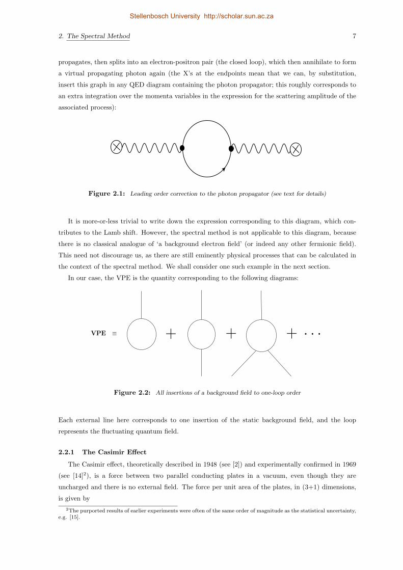
propagates, then splits into an electron-positron pair (the closed loop), which then annihilate to form
a virtual propagating photon again (the X’s at the endpoints mean that we can, by substitution,
insert this graph in any QED diagram containing the photon propagator; this roughly corresponds to
an extra integration over the momenta variables in the expression for the scattering amplitude of the
associated process):
Figure 2.1: Leading order correction to the photon propagator (see text for details)
It is more-or-less trivial to write down the expression corresponding to this diagram, which con-
tributes to the Lamb shift. However, the spectral method is not applicable to this diagram, because
there is no classical analogue of ‘a background electron field’ (or indeed any other fermionic field).
This need not discourage us, as there are still eminently physical processes that can be calculated in
the context of the spectral method. We shall consider one such example in the next section.
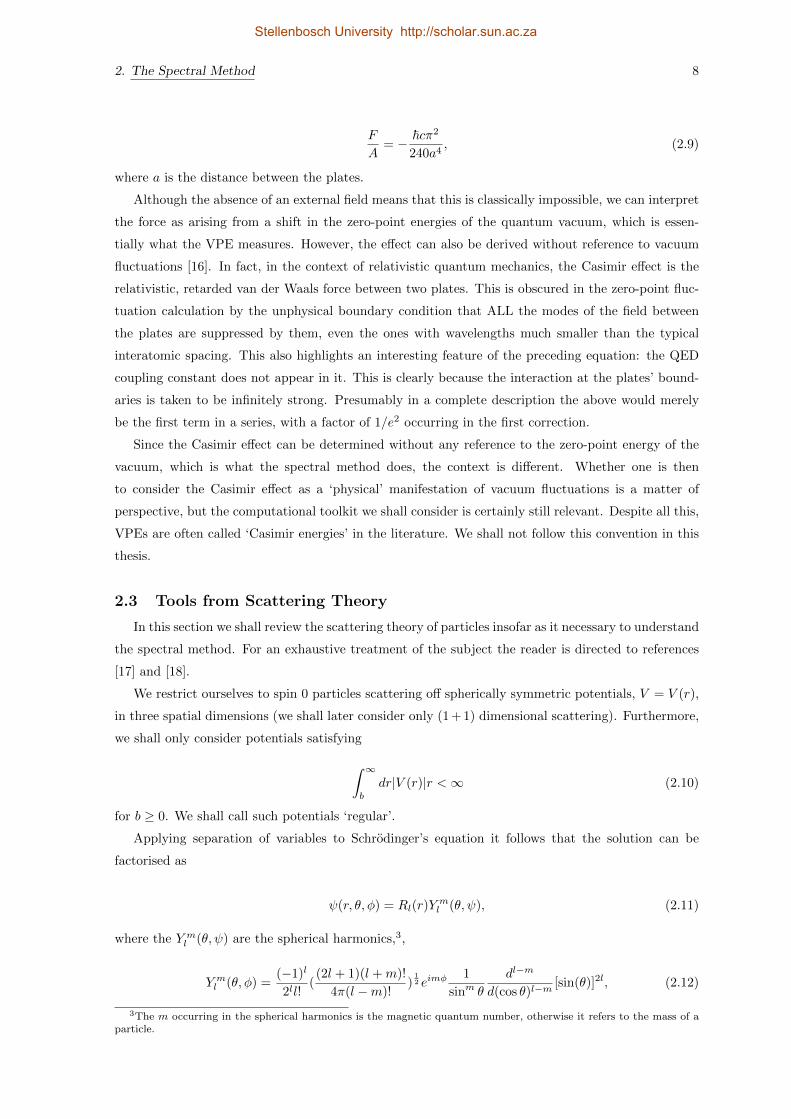
In our case, the VPE is the quantity corresponding to the following diagrams:
+ + + . . .VPE ≡
Figure 2.2: All insertions of a background field to one-loop order
Each external line here corresponds to one insertion of the static background field, and the loop
represents the fluctuating quantum field.
2.2.1 The Casimir Effect
The Casimir effect, theoretically described in 1948 (see [2]) and experimentally confirmed in 1969
(see [14]2), is a force between two parallel conducting plates in a vacuum, even though they are
uncharged and there is no external field. The force per unit area of the plates, in (3+1) dimensions,
is given by
2The purported results of earlier experiments were often of the same order of magnitude as the statistical uncertainty,e.g. [15].
Stellenbosch University http://scholar.sun.ac.za
2. The Spectral Method 8
F
A= − ~cπ2
240a4, (2.9)
where a is the distance between the plates.
Although the absence of an external field means that this is classically impossible, we can interpret
the force as arising from a shift in the zero-point energies of the quantum vacuum, which is essen-
tially what the VPE measures. However, the effect can also be derived without reference to vacuum
fluctuations [16]. In fact, in the context of relativistic quantum mechanics, the Casimir effect is the
relativistic, retarded van der Waals force between two plates. This is obscured in the zero-point fluc-
tuation calculation by the unphysical boundary condition that ALL the modes of the field between
the plates are suppressed by them, even the ones with wavelengths much smaller than the typical
interatomic spacing. This also highlights an interesting feature of the preceding equation: the QED
coupling constant does not appear in it. This is clearly because the interaction at the plates’ bound-
aries is taken to be infinitely strong. Presumably in a complete description the above would merely
be the first term in a series, with a factor of 1/e2 occurring in the first correction.
Since the Casimir effect can be determined without any reference to the zero-point energy of the
vacuum, which is what the spectral method does, the context is different. Whether one is then
to consider the Casimir effect as a ‘physical’ manifestation of vacuum fluctuations is a matter of
perspective, but the computational toolkit we shall consider is certainly still relevant. Despite all this,
VPEs are often called ‘Casimir energies’ in the literature. We shall not follow this convention in this
thesis.
2.3 Tools from Scattering Theory
In this section we shall review the scattering theory of particles insofar as it necessary to understand
the spectral method. For an exhaustive treatment of the subject the reader is directed to references
[17] and [18].
We restrict ourselves to spin 0 particles scattering off spherically symmetric potentials, V = V (r),
in three spatial dimensions (we shall later consider only (1 + 1) dimensional scattering). Furthermore,
we shall only consider potentials satisfying
∫ ∞
b
dr|V (r)|r <∞ (2.10)
for b ≥ 0. We shall call such potentials ‘regular’.
Applying separation of variables to Schrodinger’s equation it follows that the solution can be
factorised as
ψ(r, θ, φ) = Rl(r)Yml (θ, ψ), (2.11)
where the Y ml (θ, ψ) are the spherical harmonics,3,
Y ml (θ, φ) =(−1)l
2ll!((2l + 1)(l +m)!
4π(l −m)!)
12 eimφ
1
sinm θ
dl−m
d(cos θ)l−m[sin(θ)]2l, (2.12)
3The m occurring in the spherical harmonics is the magnetic quantum number, otherwise it refers to the mass of aparticle.
Stellenbosch University http://scholar.sun.ac.za

2. The Spectral Method 9
and wl ≡ rRl(r) satisfies the reduced radial Schrodinger equation4
− d2wldr2
+ [V (r) +l(l + 1)
r2]wl = Ewl. (2.13)
We note that this is identical to the time independent Schrodinger equation but with an extra term in
the effective potential that tends to throw the particle outwards. The l’s are the angular momentum
quantum numbers.
The usual approach in potential scattering theory is to look for asymptotic solutions (i.e. solutions
‘far away’, where the effect of the potential can be ignored). One possible solution in the asymptotic
regime is the combination of an incoming plane wave and an outgoing spherical wave at infinity,
namely
limr→∞
[ψ(r, θ, φ)− (ei~k·~r +A(θ, φ)
eikr
r)] = 0. (2.14)
The second, linearly independent, solution is obtained by complex conjugation and parameterisation
of an incoming spherical wave.
The function A(θ, φ)5, the amplitude of the outgoing wave, is called the scattering amplitude and
leads to the probability of a particle being scattered in a certain direction, normalised with respect to
the incoming flux:
dσ
dΩ= |A(θ, φ)|2. (2.15)
This quantity is called the scattering cross-section, and plays a central role in the experimental
scattering of particles.
2.3.1 Phase shifts and the S-matrix
Since the spherical harmonics form a complete orthonormal basis we can expand the scattering am-
plitude in terms of them. For any arbitrary function of the polar and azimuthal angles, g(θ, φ), we
have
g(θ, φ) =∑
l,m
cl,mYml (θ, φ). (2.16)
Examining the explicit formula for the spherical harmonics, and noting that the scattering ampli-
tude for a spherically symmetric potential has no φ dependence, we see that all the m terms contribute
equally to the sum in equation (2.16), yielding a degeneracy factor of (2l+ 1), so that for a potential
V (r) the scattering amplitude is
A(θ) =
∞∑
l=0
(2l + 1)al(k)Pl(cos θ), (2.17)
where the a′ls are as yet to be determined expansion coefficients and the Pl(cos θ) are Legendre
polynomials. The incoming plane wave can be expanded similarly,
4Reduced units, ~ = 1 and 2m = 1 (with m here the mass), are used throughout this section.5The angles θ and φ are measured with respect to ~k.
Stellenbosch University http://scholar.sun.ac.za
2. The Spectral Method 10
ei~k·~r = eikr cos θ =
∞∑
l=0
(2l + 1)iljl(kr)Pl(cos θ) (2.18)
with jl a spherical Bessel function, which is a solution of (2.13) for the free case (i.e. V (r) = 0).
Considering the asymptotic behaviour of jl,
limr→∞
[iljl(kr)−eikr − e−i(kr−lπ)
2ikr] = 0 (2.19)
and inserting (2.18) and (2.17) in the ansatz (2.14) we get the asymptotic behaviour of the solution
to the Schrodinger equation (2.11) for a radially symmetric potential as
limr→∞
(ψ(r, φ)−∞∑
l=0
(2l + 1)Pl(cos θ)
2ik[(1 + 2ikal(k))
eikr
r− e−i(kr−lπ)
r]) = 0. (2.20)
This may be interpreted to mean that the scattering potential changes the coefficient of the outgoing
wave by 1 + 2ikal(k). We can use this to define the S-matrix element
Sl(k) ≡ e2iδl(k) ≡ 1 + 2ikal(k). (2.21)
The factor of two in the exponent is purely due to convention. The functions δl(k) are called the
phase shifts. They play an important role in the spectral method, as we shall see.
We motivate here why we can define the S-matrix elements as pure phases. Intuitively the S-matrix
is a representation of an operator that connects free states in the asymptotic past (‘in’ states) to
states in the far future (‘out’ states). Since the Hamiltonian of a system with a spherically symmetric
potential is itself rotationally invariant we know from Noether’s theorem that angular momentum
must be conserved. This is equivalent to requiring the S-matrix to be diagonal in the representation
with angular momentum eigenkets as basis vectors. The hermiticity of the Hamiltonian, which is
required for a sensible interpretation of quantum mechanics, forces the S-matrix to be unitary (via
probability conservation). Then its eigenvalues (which are just the diagonal matrix entries) must have
a magnitude of unity, so equation (2.21) is a valid parameterisation. We shall see later, in chapter 4,
how to generalise these notions to two-channel scattering with a mass gap, in which case we shall deal
with a conceptually simple 2× 2 S-matrix.
2.3.2 The regular and Jost solutions
The free solution to the radial Schrodinger equation (2.13) is
ul(kr) = krψl(kr) = (πkr
2)
12 Jl+ 1
2(kr), (2.22)
where J is now the ordinary, not spherical, Bessel function. The general solution to the radial equation
is a linear combination of spherical Bessel and von Neumann functions, but the spherical von Neumann
function is singular at r = 0 and must be excluded if the origin is included to avoid unnormalisable
wave functions. The asymptotic behaviour of (2.22) is
limr→∞
[ul(kr)− sin(kr − lπ
2)] = 0, (2.23)
Stellenbosch University http://scholar.sun.ac.za

2. The Spectral Method 11
so that we regain the interpretation of the scatterer introducing phase shifts.
We define the regular solution, φl(k, r), by the boundary condition
limr→0
(2l + 1)!!r−l−1φl(k, r) = 1. (2.24)
The existence of such a solution is guaranteed [17] if we consider regular potentials like (2.10). (Note
that this boundary condition, unlike that of the ‘physical’ wave function ψl(k, r), is k independent).
Intuitively (2.24) means that the potential must be less singular than 1r near the origin. It is known
that the regular solution is the only one which vanishes at the origin [18] and since this is also required
of the physical solution it must be a multiple of the regular solution.
We introduce the Jost solution to the radial Schrodinger equation as fl(k, r) with the boundary
condition
limr→∞
(fl(k, r)− eilπ2 eikr) = 0 (2.25)
and
limr→∞
(f ′l (k, r)− ikeilπ2 eikr) = 0, (2.26)
where the prime denotes differentiation with respect to the spatial coordinate. The Wronskian of two
functions is defined by
W (a, b) ≡ ab′ − ba′. (2.27)
If a and b are solutions to the reduced radial Schrodinger equation then
d
drW (a, b) = 0. (2.28)
The above then allows us to see that
W [fl(k, r), fl(−k, r)] = 2ik(−1)l+1, (2.29)
which indicates linear independence6 for k 6= 0. Since there are only two linearly independent solutions
of a second order differential equation the regular solution must be expressible as a linear combination
of the Jost solutions (at least for k 6= 0). Defining the Jost function
Fl(k) = (−k)lW [fl(k, r), φl(k, r)] (2.30)
we can write the regular solution as
φl(k, r) =1
2ik−l−1[Fl(k)fl(−k, r)− (−1)lFl(−k)fl(k, r)]. (2.31)
We state a number of properties and results (see ref. [17]) that will be relevant in the context of
the spectral method:
1. The phase shift is equal to minus the phase of the Jost function
6This is a result of a theorem that says that two functions are linearly independent where their Wronskian does notdisappear, as long as they have continuous first derivatives on that interval.
Stellenbosch University http://scholar.sun.ac.za
2. The Spectral Method 12
2. Fl(−k) = [Fl(k)]∗ and Fl(−k) = |Fl|eiδl(k) ∀k ∈ R
3. lim|k|→∞
Fl(k) = 1
4. Fl(k) is analytic in the upper complex k-plane and has zeros on the positive imaginary axis
corresponding to bound states, k = iκ, so that E = −κ2 in the non-relativistic case (and these
are all the bound states)
5. These zeros are finite in number and simple (except for l ≥ 1 and Fl(0) = 0, in which case the
zero at the origin would be double, i.e. then there is a pole of second order at r = 0 and a true
bound state at E = 0)
6. For real k the phase shifts are given by δl(k) = 12i lnSl(k) = 1
2i [lnFl(−k) − lnFl(k)] (this
statement is equivalent to item 2 above)
7. The phase shifts are odd for real k.
2.3.3 Levinson’s Theorem
An important result which we shall need in the calculation presented in section 2.4 is Levinson’s
theorem, first published in 1949 [19]. A proof for the s-wave (l = 0) is presented in appendix A. The
statement of the theorem is that for potentials of type (2.10), that permit n bound states, we have
δ(0)− δ(∞) =
nπ if Fl(0) 6= 0
π(n+ 12 ) if Fl(0) = 0.
(2.32)
The convention is to take δ(∞) = 0. This reflects the fact that we do not expect a particle with
infinite energy to be perturbed by a regular potential, and is equivalent to requiring the S-matrix to
go to unity for large momenta.
This rather elegant result is of wide utility. If one is calculating the phase shift numerically, it is
immediately obvious in which regime(s) a bound state appears. On the other hand, in certain analytic
calculations involving integrals, it is convenient to perform integration by parts, which Levinson’s
theorem greatly facilitates. We shall later consider the scattering of two particles off a potential, in
which case the quantity of interest will be the sum of the phase shifts of the diagonalised S-matrix.
Even then, if the theory has a mass gap, we expect that a phase shift of some integer multiple of π
inside this mass gap at threshold, where the energy equals the mass of the lighter field, will indicate
the presence of a bound state below the mass gap when the off-diagonal coupling is omitted. We shall
numerically investigate this issue later, in section 5.3, where we shall see that it provides evidence for
the analyticity of the Jost function.
2.3.4 Density of states
The density of states plays an important role in the example provided in the next section. Intu-
itively it measures the number of states available in a given energy interval. We are only interested in
the difference between the free and interacting density of states. We motivate the form of this quantity
Stellenbosch University http://scholar.sun.ac.za

2. The Spectral Method 13
by putting the system in a ‘box’ (in one spatial dimension) and considering the antisymmetric channel
for simplicity.
In the free case the solution for the small oscillation modes is φk(r) = sin kr. In the presence of a
potential we expect the solution to approach this one asymptotically, but with a possible phase shift,
limr→∞
φk(r) sin−1(kr + δ(k)) = 1. (2.33)
Since the phase shift is only defined modulo π, we require it to be a continuous function of k that
disappears as k →∞.
We then place the system in a ‘box’ by enforcing the boundary conditions φk(0) = φk(L) = 0, for
some large L. This yields a discrete spectrum of allowed values of k, which we can enumerate as
...
kn+1L+ δ(kn+1) = (n+ 1)π
knL+ δ(kn) = nπ
... (2.34)
Next, we subtract the lower line from the upper, and divide by π(kn+1 − kn). If we assume that
this last term is sufficiently small we can approximate the difference in phase shifts by a derivative,
1
π
(L+
dδ(k)
dk
)=
1
kn+1 − kn. (2.35)
We see that the right hand side is the inverse of the momentum spacing between the states, i.e. the
density of states.
We would like to take the continuum limit L→∞. However, the density of states in the equation
above diverges in this limit as the momentum spacing becomes infinitely small. This can remedied by
considering the difference between the density of states of the interacting and free systems,
∆ρ(k) ≡ ρ(k)− ρ(0)(k) =1
π
dδ(k)
dk. (2.36)
This quantity is finite. In higher spatial dimensions there may be additional degeneracy factors and a
sum over partial waves (in one spatial dimension the analogue of angular momentum numbers are the
odd and even channels, corresponding to antisymmetric and symmetric wavefunctions, respectively).
A more rigorous definition makes use of the Green’s function Gl(r, r′, k) so that
∆ρ(k) ≡ 2k
πIm
∫ ∞
0
dr[Gl(r, r, k + iε)−G(0)l (r, r, k + iε)]. (2.37)
Here the superscript refers to the free Green’s function. There are a number of alternative represen-
tations which are not immediately relevant to us. The actual form of the Green’s function is also not
of any immediate consequence for the illustration of the example of one scalar field which is to follow:
it is sufficient that it exists as a solution to the inhomogeneous differential equation corresponding to
the relevant particle equation(s) of motion. The interested reader is directed to reference [20]. We
shall, in a later section, study the Green’s function for two channel scattering in more detail.
Stellenbosch University http://scholar.sun.ac.za
2. The Spectral Method 14
2.4 Motivational Example
Let us consider what is perhaps the simplest example possible to illustrate the concepts outlined
above: a scalar field in (1 + 1) dimensions7. A number of the expressions we shall use are purely
formal, in the sense that they may require regularisation. Nonetheless, we shall demonstrate how the
spectral method allows physically meaningful information to be extracted from such expressions.
2.4.1 Lagrangian density and energy differences
The Lagrangian density of a Klein-Gordon field coupled to a static (i.e. time independent) and
symmetric background potential is
L =1
2[(∂µφ)2 −m2φ2 − V (r)φ2]. (2.38)
After the fields are quantised we are left with an infinite set of harmonic oscillators. Specifically,
each normal mode φi is associated with a pair of creation/annihilation operators that respectively
increment/decrement the occupation number ni of that mode. The energy of each mode is
Ei = ωi(ni +1
2), (2.39)
where ωi is the energy of mode i.
We immediately see that the naive vacuum, where ni = 0 ∀i, still has the divergent energy
E =1
2
∑
i
ωi. (2.40)
Another serious problem is that this expression is not really a sum, since we may need to include
the energy of the continuum of scattering states in the form of an integral. The rest of this section
deals with the appropriate way of extracting useful physical information from this divergent quantity.
This will involve introducing the machinery from scattering theory necessary to rewrite (2.40) in a
numerically tractable form.
We begin with the observation that in QFT, in contrast to General Relativity, we are only interested
in energy differences, so that we define the quantity of interest to be
∆E ≡ 1
2
∑
i
ωi −1
2
∑
i
ω(0)i + ECT , (2.41)
where ECT is the counterterm contribution. This expression is then the difference in vacuum energy
between the full and free (i.e. where V (r) = 0) theories. While we may naively attempt to apply
normal-ordering to get rid of this infinite constant, this would overlook the fact that the first two
terms in expression (2.41) refer to different vacua. We may normal order the first term with respect
to the true vacuum of the full theory, thus getting rid of this zero-point energy, but the second term
will then not be normal ordered with respect to the non-interacting vacuum, which is the relevant
state.
We now apply the tools discussed in the previous section to rewrite (2.41) as a sum over a finite
7The example in this section closely follows the discussion in chapters 1 and 3 of [3].
Stellenbosch University http://scholar.sun.ac.za

2. The Spectral Method 15
number of bound states and an integral weighted by the difference between the density of states in
the free and interacting cases. The result is
∆E =b.s.∑
j
1
2ωj +
1
2π
∫ ∞
0
dkωdδ(k)
dk+ ECT , (2.42)
where the ωj are the bound state energies, ωj =√m2 − κ2
i . We immediately note that, since the phase
shift δ(k) goes like 1k as k tends to infinity, the second term is still divergent, and so is the counterterm
contribution. However, if the renormalisation scheme is to be consistent their combination must be
finite. We need to choose a suitable regularisation for the combination of the two. The logarithmic
divergence corresponds to the usual divergence of a scalar field theory in (1 + 1) dimensions. We use
Levinson’s Theorem (see section 2.3.3 ) to write the above as
∆E =b.s.∑
j
1
2(ωj −m) +
1
2π
∫ ∞
0
dk(ω −m)dδ(k)
dk+ ECT . (2.43)
The integral is still divergent. However, recalling that the Born approximations to the phase shifts
are exact at large k, we subtract the first Born approximation to the phase shift to obtain the finite
expression
∆E =b.s.∑
j
1
2(ωj −m) +
1
2π
∫ ∞
0
dk(ω −m)d
dk[δ(k)− δ(1)(k)] + ECT + EFD. (2.44)
We have added the Born subtraction back in the form of a Feynman diagram, EFD. This is legitimate
because terms of the Born series can be identified with Feynman diagrams, as we shall see in the next
section.
Applying integration by parts to the second term in the previous equation yields
1
2π
∫ ∞
0
dk(ω −m)d
dk[δ(k)− δ(1)(k)] =
1
2π(ω −m)[δ(k)− δ(1)(k)] |∞0 −
1
2π
∫ ∞
0
dkk
ω[δ(k)− δ(1)(k)]
= − 1
2π
∫ ∞
0
dkk
ω[δ(k)− δ(1)(k)]. (2.45)
The first two terms in the first line fall away because the Born approximation is exact as k →∞, so
that δ(∞) = δ(1)(∞), and there are no bound states in the Born approximation, so that δ(n)(0) = 0
for all n, from Levinson’s theorem. It is also the case that ω = m if k = 0.
After putting this all together, equation (2.44) becomes
∆E =1
2
b.s.∑
j
(ωj −m)− 1
2π
∫ ∞
0
dkk
ω[δ(k)− δ(1)(k)] + ECT + EFD. (2.46)
This expression is numerically very tractable. Furthermore, standard techniques from perturbative
QFT can be applied to the sum ECT +EFD. For a scalar theory in (1 + 1) dimensions, only the local
tadpole diagram occurs, and ECT + EFD = 0. This is the general procedure in the spectral method:
Subtract as many Born-approximations to the phase shift as are necessary to regularise the integrals,
then add back the subtracted piece(s) via Feynman diagrams, which can be renormalised by the usual
method of adding counterterms to the Lagrangian. For instance, if we repeat the preceding analysis
Stellenbosch University http://scholar.sun.ac.za
2. The Spectral Method 16
for a single fermion field in (1 + 1) dimensions we find that two Born subtractions are necessary to
render the relevant integral finite. It is clear that the application of this procedure is only valid when
the underlying theory is renormalisable, so that the sum ECT + EFD is finite. The following section
contains a proof that the terms of the Born series can be identified with Feynman diagrams.
2.4.2 The relationship between Feynman diagrams and terms of the Born series
The vacuum to vacuum transition amplitude for a field φ in d spatial dimensions coupled to the
background field V (x) is given by
⟨Ω+|Ω−
⟩V∝ (det[∂µ∂
µ +m2 + V − iε])− 12 , (2.47)
where |Ω+〉 and |Ω−〉 refer to the vacuum states at t = +∞ and t = −∞ respectively. This means
that we are considering a scenario where the interaction V (x) is adiabatically ‘switched on’ at an early
time −T2 , and ‘switched off’ at time +T2 .
The energy density operator is the vacuum expectation value of the component T00 of the energy
momentum tensor, ε(x) ≡ 〈0| T00 |0〉. For a single field φ coupled to the background V (x) we have8
ε(x) =1
2
∫[dφ]φ(x)Txφ(x)ei
∫ddy 1
2 [φ2−(∂φ)2−(m2+V )φ2]
∫[dφ]ei
∫ddy 1
2 [φ2]−(∂φ)2−(m2−V )φ2, (2.48)
where Tx is the position space operator defined by
Tx ≡←−∂0−→∂0 +
←−∂ · −→∂ +m2 + V (x). (2.49)
We would like to compute the vacuum expectation value of T00, as it occurs above. We note that the
expression is quadratic in the field φ, so we add an interaction that couples it linearly to a source,
compute the logarithmic derivative with respect to that source, and then set the source equal to zero9.
We then have
ε(x) =i
2Tr[−∂µ∂µ − (m2 + V )]−1δd(x− x)[−∂2
0 − ∂2 + (m2 + V )] (2.50)
= −iTr[[−∂µ∂µ − (m2 + V )]−1δd(x− x)∂20 ] + ..., (2.51)
where the ellipsis in the last line refers to contributions that do not involve V , and the notation
Tr includes space-time integration. We note that the free propagator is S0 = [−∂µ∂µ − m2]−1, so
[−∂µ∂µ − (m2 + V )]−1 = [1− S0V ]−1S0. Since V is static, we can introduce the frequency states |ω〉that satisfy 〈ω|V |ω′〉 = V δ(ω − ω′). Then the νth order term in the Feynman series of the energy
density is
ε(ν)FD(x) = i
∫dω
2πTr′[ω2(S0(ω)V )νS0(ω)δd−1(x− x)], (2.52)
where S0(ω) = (ω2 + ∂2 −m)−1 and Tr′ refers to the trace over the remaining degrees of freedom.
Since this expression gives the O(V ν) contribution to the energy density, we are justified in associating
it with the Feynman diagram (with ν external legs) contribution to the energy density (up to total
8The following is from chapters 3.3 and 3.5 of [3], which can be consulted for further details.9See chapters 5 and 6 of [21] for a general overview of this method.
Stellenbosch University http://scholar.sun.ac.za
2. The Spectral Method 17
derivatives that will not contribute to the integrated density).
2.4.3 Renormalisation of the tadpole graph
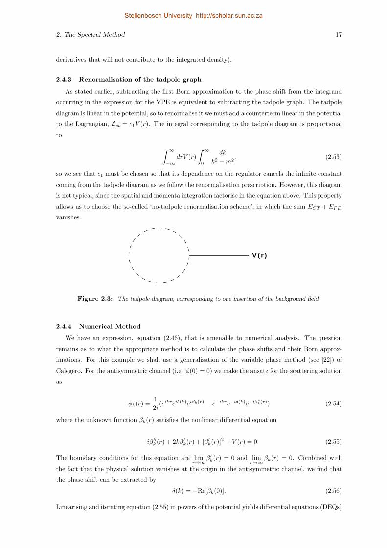
As stated earlier, subtracting the first Born approximation to the phase shift from the integrand
occurring in the expression for the VPE is equivalent to subtracting the tadpole graph. The tadpole
diagram is linear in the potential, so to renormalise it we must add a counterterm linear in the potential
to the Lagrangian, Lct = c1V (r). The integral corresponding to the tadpole diagram is proportional
to
∫ ∞
−∞drV (r)
∫ ∞
0
dk
k2 −m2, (2.53)
so we see that c1 must be chosen so that its dependence on the regulator cancels the infinite constant
coming from the tadpole diagram as we follow the renormalisation prescription. However, this diagram
is not typical, since the spatial and momenta integration factorise in the equation above. This property
allows us to choose the so-called ‘no-tadpole renormalisation scheme’, in which the sum ECT + EFD
vanishes.
V ( r )
Figure 2.3: The tadpole diagram, corresponding to one insertion of the background field
2.4.4 Numerical Method
We have an expression, equation (2.46), that is amenable to numerical analysis. The question
remains as to what the appropriate method is to calculate the phase shifts and their Born approx-
imations. For this example we shall use a generalisation of the variable phase method (see [22]) of
Calegero. For the antisymmetric channel (i.e. φ(0) = 0) we make the ansatz for the scattering solution
as
φk(r) =1
2i(eikreiδ(k)eiβk(r) − e−ikre−iδ(k)e−iβ
∗k(r)) (2.54)
where the unknown function βk(r) satisfies the nonlinear differential equation
− iβ′′k (r) + 2kβ′k(r) + [β′k(r)]2 + V (r) = 0. (2.55)
The boundary conditions for this equation are limr→∞
β′k(r) = 0 and limr→∞
βk(r) = 0. Combined with
the fact that the physical solution vanishes at the origin in the antisymmetric channel, we find that
the phase shift can be extracted by
δ(k) = −Re[βk(0)]. (2.56)
Linearising and iterating equation (2.55) in powers of the potential yields differential equations (DEQs)
Stellenbosch University http://scholar.sun.ac.za
2. The Spectral Method 18
from which the Born approximations to the phase shifts can be computed. For instance, to first order
in V (r),
− iβ′′(1)k (r) + 2kβ
′(1)k (r) + V (r) = 0, (2.57)
from which we can, together with the appropriate boundary conditions, extract
δ(1)(k) = −Re[β(1)k (0)]. (2.58)
This expression allows us to numerically determine the VPE of this simple model to arbitrary precision,
in the antisymmetric channel. To calculate the complete VPE it is necessary to sum over both channels,
but for the purpose of illustration it is sufficient to consider only the antisymmetric channel.
We shall later see in section 4.4 how this approach can be modified to deal with the case of two
fields that are scattering, where the quantity of interest is the sum of the phase shifts in the two
channels.
Stellenbosch University http://scholar.sun.ac.za
3 Scattering solution for two interacting scalar fields
In this chapter we provide an example of how scattering methods can be applied to two coupled fields
in the context of QFT. This serves both to introduce some useful conceptual tools from field theory,
and to motivate the calculation of the VPE of two interacting scalar fields which occurs later.
Consider the Lagrangian density
L = L1 + L2 + Lcoupling, (3.1)
where
1. L1 = 12∂µφ∂
µφ− λ4 (φ2 − m2
1
λ )2
2. L2 = 12∂µψ∂
µψ − m22
2 ψ2
3. Lcoupling = gψ(φ2 − m21
λ )2,
which describes two fields with densities L1 and L2 interacting via Lcoupling. Here m2 >√
2m1 and
g is a coupling constant. The φ occurring in this equation should not be confused with the regular
solution.
We shall consider a static (i.e. time independent) soliton solution of L1 that satisfies the classical
equation of motion and expand around this, quantising the small oscillation field η which will be
introduced shortly. This is equivalent to assuming that the fields commute, and calculating the O(~)
corrections to the result obtained from this assumption. We shall then rewrite this as a matrix
scattering equation.
3.1 Expansion around a static solution
We begin by considering fluctuations around a static solution of L1 which satisfies the Euler-
Lagrange equation of motion in one spatial dimension,
∂2rφ = λφ(φ2 − m2
1
λ). (3.2)
We consider specifically the stationary kink solution
φk =m1√λ
tanh(m1√
2r), (3.3)
which is a soliton [23] that reduces to the vacua ± m1√λ
at positive/negative spatial infinity (we say
that the solution interpolates between these two vacua). Defining the current
Jµ =
√λ
m1εµν∂νφk (3.4)
19
Stellenbosch University http://scholar.sun.ac.za

3. Scattering solution for two interacting scalar fields 20
we see that we have a conserved (i.e. ∂µJµ = 0) topological ‘charge’
Q =1
2
∫ ∞
−∞drJ0 =
1
2
m1√2
∫ ∞
−∞dr sech2(
m1√2r) = 1 (3.5)
for φk10. The conservation implies that this solution is topologically stable, in the sense that it cannot
continuously decay to a solution with charge Q that differs from its initial value, as this would require
infinite energy. We then look for solutions to small fluctuations around this field, i.e. solutions of L1
with
φ = φk + η. (3.6)
After quantisation, these fluctuations η about the classical solution correspond to bosons with the
mass of the lighter field φ.
To facilitate the use of results from scattering theory, we expand the complete Lagrangian to
quadratic order in η,
L =1
2∂µη∂
µη +1
2∂µψ∂
µψ − m22
2ψ2 − λ
4η2(6φ2
k −2m2
1
λ) + 4gφk(φ2
k −m2
1
λ)ψη (3.7)
which yields the Euler-Lagrange equations for the fields ψ and η respectively as
∂µ∂µψ = −m2
2ψ + 4gφk(φ2k −
m21
λ)η (3.8)
and
∂µ∂µη = 4gφk(φ2
k −m2
1
λ)ψ − λ
2(6φ2
k −2m2
1
λ)η. (3.9)
We can write this more succinctly as
∂µ∂µ
ψ
η
=
−m22 4gφk(φ2
k −m2
1
λ )
4gφk(φ2k −
m21
λ ) −λ2 (6φ2k −
2m21
λ )
ψ
η
. (3.10)
We shall refer to this as the small oscillation equation.
The 2 × 2 matrix on the right hand side has the virtue of becoming a diagonal matrix as r → ∞because of the properties of the soliton solution φk. Specifically, it becomes the mass matrix
−m2
2 0
0 −2m21
. (3.11)
We interpret this fact to mean that equation (3.10) describes asymptotically free scalar fields.
3.2 Regular solution in one channel
It is necessary at this point to return briefly to potential scattering theory in one spatial dimension.
Specifically, for s-wave the boundary conditions for the regular solution become φ(k, 0) = 0 and
φ′(k, 0) = 1. We can use this to convert the reduced radial Schrodinger equation into an integral
10Note that Jµ is conserved despite not being a Noether current.
Stellenbosch University http://scholar.sun.ac.za

3. Scattering solution for two interacting scalar fields 21
equation (by the method of Green’s functions) to obtain a Volterra integral of the second kind. We
construct the Green’s function explicitly as follows: The solution to the free equation (which is just
the Helmholtz equation in one spatial dimension) satisfies11
(∂2r + k2)φ(0)(k, r) = 0. (3.12)
The solution is
φ(0)(k, r) = c1 cos(kr) + c2 sin(kr), (3.13)
which the boundary conditions force to be
φ(0)(k, r) =sin(kr)
k. (3.14)
We note that if we ignore for the moment the fact that the delta function is actually a distribution, and
hence only properly defined under an integral sign, the Green’s function Gk(r) satisfies, by definition,
(∂2r + k2)Gk(r) = δ(r), (3.15)
and that this allows us to express φ(k, r) as
φ(k, r) = φ(0)(k, r) +
∫ r
0
dr′Gk(r − r′)V (r′)φ(r′), (3.16)
since
(∂2r + k2)φ(k, r) =
∫ r
0
dr′δ(r − r′)V (r′)φ(r′)
= V (r)φ(k, r). (3.17)
Explicit computation verifies that the appropriate Green’s function is
Gk(r − r′) =sin k(r − r′)
kθ(r′ − r), (3.18)
so that we are led to the regular solution,
φ(k, r) =sin(kr)
k+
∫ r
0
dr′sin k(r − r′)
kV (r′)φ(k, r′). (3.19)
Substitution of this equation in (2.13) verifies that this is indeed the integral version of that equation
(for l = 0).
If we define (for n = 1, 2, . . . )
φ(n)(k, r) ≡∫ r
0
dr′sin k(r − r′)
kV (r′)φ(n−1)(k, r′) (3.20)
then the bounds [17]
11We use here reduced units, ~ = 1 and 2m1 = 1.
Stellenbosch University http://scholar.sun.ac.za
3. Scattering solution for two interacting scalar fields 22
∣∣∣∣sin kr′
k
∣∣∣∣ ≤ Cr′
1 + |k|r′ e|Imk|r′ , (3.21)
for r′ > 0 and complex k, and
∣∣∣∣sin k(r − r′)
k
∣∣∣∣ ≤ Cr
1 + |k|r e|Imk|(r−r′), (3.22)
for r ≥ r′ ≥ 0, allow us to see that
|φ(1)(k, r)| ≤∫ r
0
dr′∣∣∣∣sin k(r − r′)
k
∣∣∣∣ |V (r′)|∣∣∣∣sin kr′
k
∣∣∣∣
≤ C r
1 + |k|r
∫ r
0
dr′|V (r′)| r′
1 + |k|r′ e|Imk|(r−r′)e|Imk|r′
= Cr
1 + |k|r e|Imk|r
∫ r
0
dr′|V (r′)| r′
1 + |k|r′ , (3.23)
where C is a numerical value independent of k or r. Iterating this calculation yields the general bound
|φ(n)(k, r)| ≤ C r
1 + |k|r e|Imk|r 1
n!
[C
∫ r
0
dr′r′
1 + |k|r′ |V (r′)|]n
(3.24)
for arbitrary complex k. This implies that the series
φ(k, r) =∞∑
n=0
φ(n)(k, r) (3.25)
is absolutely and uniformly convergent in any compact subset of the complex k-plane (and hence the
unique solution to (3.19)) as long as the potential is regular. It is therefore important to keep in
mind that the name regular solution is something of a misnomer for equation (3.19), as it is simply
the radial Schrodinger equation, subject to specific boundary conditions, that we have rewritten as
an integral equation. Its actual solution would depend on as many terms of equation (3.25) as are
needed to achieve the desired level of precision.
A very similar argument, using the same inequalities as above and an additional step which can
be found in reference [17], shows that the series expansion of the Jost solution is also absolutely and
uniformly convergent, but only for Imk ≥ 0. The Jost solution also solves equation (3.12), but with
the boundary conditions (2.25) and (2.26). This is accomplished by the integral equation
f(k, r) = eikr +
∫ ∞
r
dr′sin k(r − r′)
kV (r′)f(k, r′). (3.26)
The relevant series expansion is defined by
f (0)(k, r) = eikr (3.27)
and
f (n)(k, r) = eikr +
∫ ∞
r
dr′sin k(r − r′)
kV (r′)f (n−1)(k, r′). (3.28)
Stellenbosch University http://scholar.sun.ac.za

3. Scattering solution for two interacting scalar fields 23
3.3 From the small oscillation equation to the regular solution in two chan-
nels
We shall now show how the small oscillation equation leads to a matrix equation that is analogous
to the regular solution. For two fields it seems reasonable to expect equation (2.13) to become, in one
spatial dimension and for the s-wave,
[∂2r +
k2φ 0
0 k2η
]
ψ
η
= V (r)
ψ
η
, (3.29)
where V (r) is a 2× 2 matrix. This equation has a solution equivalent to the regular solution, but now
in two channels (as can again be verified by substitution)
ψ
η
=
sin kφrkφ
sin kηrkη
+
∫ r
0
dr′
sin kφ(r−r′)kφ
0
0sin kη(r−r′)
kη
V (r′)
ψ(r′)
η(r′)
. (3.30)
Equation (3.29) can in fact be obtained from the small oscillation equation if we make the stationary
ansatz,
ψ(r, t) = ψ(r)e−iEt (3.31)
and
η(r, t) = η(r)e−iEt, (3.32)
which is equivalent to energy conservation.
Substitution of this ansatz in the small oscillation equation (3.10) yields
[∂2r +
−m22 4gφk(φ2
k −m2
1
λ )
4gφk(φ2k −
m21
λ ) −λ2 (6φ2k −
2m21
λ )
]
ψ
η
= −E2
ψ
η
(3.33)
If we recall that energy is the same in both channels, but with different momenta, we have the
dispersion relations
E2 = k2φ +m2
2 (3.34)
and
E2 = k2η + 2m2
1. (3.35)
Substitution then yields
Stellenbosch University http://scholar.sun.ac.za

3. Scattering solution for two interacting scalar fields 24
[∂2r +
k2φ 0
0 k2η
]
ψ
η
= [
−m2
2 0
0 −2m21
−
−m22 4gφk(φ2
k −m2
1
λ )
4gφk(φ2k −
m21
λ ) −λ2 (6φ2k −
2m21
λ )
]
ψ
η
(3.36)
which is of the same form as (3.29), so that (3.30) is a solution, with the first factor on the right-hand
side in the equation above playing the role of V (r). The properties of the soliton solution ensure that
this reduces to the equation describing non-interacting fields at spatial infinity.
To summarise, we have constructed a solution for small fluctuations around a static soliton con-
figuration and established that it is analogous to a two channel version of the regular solution from
scattering theory. The analytic properties of the regular solution do unfortunately not carry over
simply to the two channel case. It is easy to see why: it follows from the dispersion relations that
while, for instance, the φ channel may be analytic in the upper complex momentum plane, making
the other field’s momentum complex will produce a divergence because of the exponential increase in
sin k(r− r′). It is clear that if k1 is taken real then k2 will be purely imaginary inside the momentum
gap, 0 < k1 <√m2
2 −m21 , so this may appear to be a serious problem. Fortunately, there are ways
around this (see chapter 17.1 of [17]).
Another important issue that is relevant with regard to the numerical results is the form of the
equation which relates k1 and k2 via the energy momentum relation. Specifically, naively choosing
k2 =√k2
1 −∆m2 , where ∆m ≡√m2
2 −m21 , leads to an incorrect sign for the imaginary/real part of
k2 as k1 takes values in the complex momentum plane. To get around this issue we choose to define
k2 = k1
√1− ∆m2
k21. We must use this form of the expression in the numerical program that solves the
differential equations from which the phase shifts are extracted to avoid sign errors. More specifically,
this ensures that
sgn(k1) = sgn(k2), (3.37)
which is necessary if we want δ(k) = −δ(−k), as demanded by the properties of the phase shifts
outlined in chapter 2.
Stellenbosch University http://scholar.sun.ac.za
4 The model
In this chapter we define our model within the context of QFT, and confirm that it is self-consistent
by performing the standard calculations associated with the canonical quantisation of a field theory.
An expression for the vacuum polarisation energy is derived based on a Fock decomposition of two
interacting scalar fields. We then make a connection with the spectral method by introducing a
scattering ansatz that allows us to extract the scattering phase shifts (and the Born approximations
thereof) from certain differential equations (DEQs) that can be solved by a computer. We also describe
how the discrete binding energies enter into the calculation of the VPE, and how they can be obtained
numerically.
A concrete example of this procedure is then provided and compared to the known analytic results
for a specific uncoupled problem, with positive results.
4.1 Quantum Field Theory Formalism
4.1.1 Lagrangian density
Our model consists of two coupled (real) scalar fields, in (1 + 1) dimensions, with a mass gap
(m1 < m2) interacting via a static, spherically symmetric background potential V = V (r). We shall
use |Ω〉 to denote the vacuum of this full, interacting theory. The Lagrangian density corresponding
to two scalar fields coupled by a potential with these properties is
L =1
2(∂µΦ†∂µΦ− Φ†M2Φ− Φ†V (r)Φ), (4.1)
where we have introduced the two-component field
Φ(r, t) =
φ1(r, t)
φ2(r, t)
(4.2)
and the mass matrix
M =
m1 0
0 m2
(4.3)
for notational convenience. The radial potential that couples the two fields is likewise represented by
a 2 × 2 matrix V (r) that we leave unspecified for the moment, beyond requiring it to be Hermitian,
V †(r) = V (r).
An alternative viewpoint of our model is possible. If we consider the density of our system to be
rather
L =1
2∂µΦ†∂µΦ− 1
2Φ†M2Φ− σ(Φ), (4.4)
25
Stellenbosch University http://scholar.sun.ac.za

4. The model 26
and if φ0(r) is a stationary point of the classical action, then equation (4.1) corresponds to the
harmonic approximation
L =1
2∂µΦ†∂µΦ− 1
2Φ†M2Φ− 1
2Φ†σ′′(φ0(r))Φ + · · · (4.5)
if V (r) ≡ σ′′(φ0(r)). This makes the origin of the one-loop, or O(~), truncation of the spectral method
clear: The Φ fields describe small fluctuations about the solution φ0.
This viewpoint is of course equivalent to the preceding one. Besides its numerical efficiency, the
strength of the spectral method lies in the fact that there are no approximations made beyond the
harmonic one, so that we have a ‘non-perturbative’ method up to O(~), in the sense that it includes
all contributions from the potential, as in diagram 2.2. It is still perturbative in the sense that we
ignore effects of O(~2) and higher, so that truly non-perturbative effects cannot occur.
4.1.2 Quantisation
To quantise the system described by the Lagrangian density (4.1) above, we elevate the field Φ(r, t)
to an operator
Φ(r, t) =
φ1(r, t)
φ2(r, t)
(4.6)
that acts on the Hilbert (or Fock) space of the quantum states of the system, and enforce the equal-time
commutation relations between the field components and the components of the conjugate momenta
in the Heisenberg picture:
[φa(r, t), Πb(r′, t)] = iδ(r − r′)δab (4.7)
and between the field components at equal time:
[φa(r, t), φb(r′, t)] = 0. (4.8)
It is understood that a and b label the field components, so that these equations correspond to the
four entries in a 2× 2 matrix as the Latin indices vary over their domain.
In the present case it follows from the definition of the conjugate momenta,
Π ≡ ∂L∂(∂0Φ)
, (4.9)
that
Π = ∂0Φ†(r, t), (4.10)
i.e. in our notation it is a two-component row vector. We shall see in the next section how these
commutation relations for the fields and their conjugate momenta lead to the canonical commutation
relations (CCR) for the annihilation and creation operators.
Stellenbosch University http://scholar.sun.ac.za

4. The model 27
4.1.3 Equations of motion and canonical commutation relations
We start by assuming the stationary ansatz, so that
Φ(r, t) =
φ1(r, t)
φ2(r, t)
= Φ(r)e−iEt, (4.11)
where
E =√k2
1 +m21 . (4.12)
As a result of this, the particles associated with these fields obey the following stationary wave
equation, which should be familiar from the previous chapter:
(∂2r +K2)φ(E, r) = V (r)φ(E, r). (4.13)
It is understood that φ(E, r) is the two-component solution of this matrix differential equation, and
K2 is the 2× 2 matrix in equation (3.29) with the squared momenta on the diagonal. In the general
case the φ(E, r) occurring here can be treated as a 2 × 2 matrix. The two columns are solutions of
the equation that only differ in their boundary conditions. We shall restrict ourselves for the moment
to a specific boundary condition that will appear shortly. The alert reader will also notice that this
equation is very similar in form to the reduced radial Schrodinger equation (2.13) for the s-wave,
which, in view of the discussion in the preceding chapter, makes the applicability of scattering theory
in this context obvious. The Lagrangian density is, however, more general than that occurring there.
This stationary wave equation can be derived by applying the Euler-Lagrange equation,
∂L∂Φ− ∂µ ∂L
∂(∂µΦ)= 0, (4.14)
to the Lagrangian density (4.1) and using the stationary ansatz, as before. Following on from this,
we can define annihilation and creation operators by
aα(E) = i∑
a=1,2
∫drφ
(α)a,E(r)[∂0φa(r)− iEφa(r)]eiEt (4.15)
and
a†α(E) = −i∑
a=1,2
∫drφ
(α)∗a,E (r)[∂0φa(r) + iEφa(r)]e−iEt (4.16)
respectively. The subscript E in φ(α)a,E(r) serves to remind us that this φ(α)(r) is the Jost solution of
the stationary wave equation above at the energy E, with the subscript a labelling the component.
The φa(r) are the time independent field components.
We would like to determine all the possible commutation relations between these operators. To do
so we must first fix our normalisation. We choose the so-called covariant normalisation for the fields,
with the associated Fock decomposition as
Φ(r, t) =∑
α=1,2
∫ ∞
0
dk1
(2π)2E[
φ(α)1,E(r)
φ(α)2,E(r)
e−iEtaα(E) +
φ(α)∗1,E (r)
φ(α)∗2,E (r)
eiEta†α(E)]. (4.17)
Stellenbosch University http://scholar.sun.ac.za
4. The model 28
The Greek letter labels the two independent solutions12.
Because of the profusion of super- and sub- scripts, it will be convenient in the calculations which
will appear shortly to refer to the two column vectors occurring in the integrand above as φα,E(r)
and φ∗α,E(r). This means that φ†α,E(r)φα,E(r) is an inner product. It is hoped that this will not cause
confusion.
We expect the fields to decouple and their solutions to reduce to plane waves at spatial infinity
(that this is the case can be seen from the consideration of their Wronskian, as we shall see in the
next section), so that the vectors have the asymptotic behaviour
limr→∞
φ1,E(r)e−ik1r =
1
0
and lim
r→∞φ2,E(r)e−ik2r =
0
1
. (4.18)
The reader will notice that this is the extension of the boundary condition for the Jost solution
introduced in section 2.3.2 to two fields (and for the s-wave). We also see from the definition of the
annihilation and creation operators above that they ‘mix’ the field components.
To calculate the CCR for the model, we straightforwardly substitute equation (4.17) in the ex-
pressions for the relevant operators, and use the equal-time commutation relations from the previous
section. For example,
[a1(E), a†1(E′)] = ei(E−E′)t∑
a=1,2
∫dr
∫dr′[φ
(1)a,E(Πa(r, t)− iEφa(r, t)) , φ
(1)∗a,E′(Πa(r′, t) + iE′φa(r′, t))
]
= ei(E−E′)t∑
a=1,2
∫dr
∫dr′φ
(1)a,E(r)φ
(1)∗a,E′(r
′)(E′ + E)δ(r − r′)
= ei(E−E′)t∑
a=1,2
∫drφ
(1)a,E(r)φ
(1)∗a,E′(r)(E
′ + E). (4.19)
It is clear that if the Jost solutions φα,E(r) and φ∗α,E(r) are orthonormal,
∑
a=1,2
∫drφ
(α)a,E(r)φ
(β)∗a,E′(r) = 2πδ(k1 − k′1)δα,β , (4.20)
then the commutator above is
[a1(E), a†1(E′)] = (2π)2Eδ(k1 − k′1). (4.21)
The other cases proceed similarly, so we see that the choice of covariant normalisation, together
with the orthonormality condition for the wave solutions, lead to the canonical commutation relations
[aα(E), a†β(E′)] = (2π)2Eδ(k1 − k′1)δα,β . (4.22)
These serve to define the annihilation/creation algebra for our model. The interacting vacuum ket in
the space of the combined system is then annihilated by all the annihilation operators acting on it
12The reader may be concerned about the absence of the bound states wavefunctions. However, as we shall see in thenext section, the relevant Green’s function can be constructed to have simple poles at the bound state energies. Afterrotation to the imaginary axis the contribution from the bound state wavefunctions disappears.
Stellenbosch University http://scholar.sun.ac.za

4. The model 29
from the left,
aα(E) |Ω〉 = 0 ∀α, (4.23)
while the interacting vacuum bra in the dual space is annihilated by all creation operators acting on
it from the right,
〈Ω| a†α(E) = 0 ∀α. (4.24)
These two equations serve to define the Fock space of the system.
4.1.4 Energy density operator
The calculation of the vacuum polarisation energy requires an expression for the energy density
operator, which is the component T00 of the energy momentum tensor
Tµν =∂L
∂(∂µΦ)∂νΦ− gµνL. (4.25)
We see from this that the energy density operator is given by
T00 =1
2[∂0Φ†∂0Φ + ∂1Φ†∂1Φ + Φ†(M2 + V )Φ]. (4.26)
We can construct an expression for the vacuum polarisation energy from the spatial integral over
the energy density. The energy density is by definition the VEV of the energy density operator,
ε(r) ≡ 〈Ω| T00 |Ω〉 . (4.27)
To evaluate this expression we must first calculate T00 by inserting the Fock decomposition in (4.26).
Starting with the time derivative,
∂0Φ(r, t) =∑
α=1,2
∫ ∞
0
dk1
(2π)2E[−iE
φ(α)1,E(r)
φ(α)2,E(r)
e−iEtaα(E) + iE
φ(α)∗1,E (r)
φ(α)∗2,E (r)
eiEta†α(E)], (4.28)
so
〈Ω| ∂0Φ†∂0Φ |Ω〉 =1
4π2
∑
α,β
∫ ∞
0
dk1
∫ ∞
0
dk′1[EE′
4EE′(φ
(α)1,Eφ
(β)∗1,E′ + φ
(α)2,Eφ
(β)∗2,E′)]
× e−it(E−E′) 〈Ω| aα(E)a†β(E′) |Ω〉
=1
4π
∑
α,β
∫ ∞
0
dk1
∫ ∞
0
dk′1[E(φ(α)1,Eφ
(β)∗1,E′ + φ
(α)2,Eφ
(β)∗2,E′)]
× e−it(E−E′)δ(k1 − k′1)δα,β
=1
4π
∑
α=1,2
∫ ∞
0
dk1Eφ†α,E(r)φα,E(r). (4.29)
Stellenbosch University http://scholar.sun.ac.za
4. The model 30
Note that we have used the following ‘trick’ that follows from the commutation relations,
〈Ω| aα(E)a†β(E′) |Ω〉 = 〈Ω| [aα(E), a†β(E′)] |Ω〉 − 〈Ω| a†β(E)aα(E′) |Ω〉
= [aα(E), a†β(E′)] 〈Ω|Ω〉
= (2π)2Eδ(k1 − k′1)δα,β (4.30)
since we are free to choose an orthonormal basis so that 〈Ω|Ω〉 = I.
Similarly13,
∂1Φ(r, t) =∑
α=1,2
∫ ∞
0
dk1
(2π)2E[
φ′(α)1,E (r)
φ′(α)2,E (r)
e−iEtaα(E) +
φ′(α)∗1,E (r)
φ′(α)∗2,E (r)
eiEta†α(E)], (4.31)
so
〈Ω| ∂1Φ†∂1Φ |Ω〉 =1
4π2
∑
α,β
∫ ∞
0
dk1
∫ ∞
0
[dk′1
4EE′(φ′(α)1,E φ
′(β)∗1,E′ + φ
′(α)2,E φ
′(β)∗2,E′ )e−it(E−E
′)] 〈Ω| aα(E)a†β(E′) |Ω〉
=1
4π
∑
α=1,2
∫ ∞
0
dk1
Eφ′†α,E(r)φ′α,E(r). (4.32)
Before evaluating the last term of 〈Ω| T00 |Ω〉 we note that
φ′†α,E(r)φ′α,E(r) =1
2∂r(φ
†α,E(r)φα,E(r)′)− 1
2φ†α,E(r)φ′′α,E(r) +
1
2∂r(φ
′†α,E(r)φα,E(r))− 1
2φ′′†α,E(r)φα,E(r)
=1
2∂r(∂r(φ
†α,E(r)φα,E)(r))− φ†α,E(r)(V (r)−K2)φα,E(r), (4.33)
where we have substituted the stationary wave equation (4.13). The hermiticity of V (r) and the
symmetry of K2 ensure that the equation above holds if we take the conjugate transpose of φα,k1(r).
By a similar method
〈Ω| Φ†(M2 + V )Φ |Ω〉 =1
4π2
∑
α,β
∫ ∞
0
dk1
∫ ∞
0
dk′11
4EE′φ†α,E(r)(M2 + V )φβ,E′(r)e
−it(E−E′)
× 〈Ω| aα(E)a†β(E′) |Ω〉
=1
4π
∑
α=1,2
∫ ∞
0
dk1
Eφ†α,E(r)(M2 + V )φα,E(r). (4.34)
Combining this with equations (4.32), (4.33) and (4.34) we have the expression for the energy density
as
ε(r) =1
4π
∑
α=1,2
∫ ∞
0
dk1E(1 +∂2r
4E2)φ†α,E(r)φα,E(r) + bound state piece. (4.35)
13Primed dependent variables in the following equations denote ordinary differentiation with respect to the spatialcoordinate.
Stellenbosch University http://scholar.sun.ac.za

4. The model 31
4.2 Extension of scattering theory to two coupled fields
We now introduce the Green’s function by
G(r, r′, k1) = − 2
π
∑
α=1,2
∫ ∞
0
dqφα,q(r)⊗ φ†α,q(r′)
(k1 + iε)2 − q2+ bound state piece. (4.36)
The iε prescription leads to this Green’s function being meromorphic in the upper complex k1-plane,
with poles at the bound state energies on the imaginary axis. Recalling the notation introduced
previously, the factor like φ⊗φ† is a tensor product, so the Green’s function is matrix-valued (it is in
fact a 2× 2 matrix).
This matrix Green’s function must satisfy, by definition, the following equation of the interacting
fields,
[∂2r +K2 − V (r)]G(r, r′, k1) = I2δ(r − r′). (4.37)
We need to generalise the notions of the Jost and regular solutions discussed in section 2.3 to
matrices. To do so, we recognise that the appropriate extension of the definition of the Wronskian to
matrices is
W (A,B) ≡ ATB′ −A′TB
=
∣∣∣∣∣∣∣
AT A′T
B B′
∣∣∣∣∣∣∣. (4.38)
The introduction of the transpose is necessary to ensure that the Wronskian of two different matrix
solutions of the particle equation of motion be constant [17]. This in turn ensures that these two
solutions are linearly independent. If we take A to be one of these matrix solutions, we have W (A,A) =
ATA′ −A′TA, which we may suspect is some non-zero quantity. However,
W ′(A,A) = ATA′′ −A′′TA
= ATCA−ATCA
= 0, (4.39)
where C = −V (r) +K2. So even if W (A,A) 6= 0, it will still be independent of r. If this solution A
is the Jost solution, then we know that it becomes diagonal in the limit as r → ∞, and this implies
that the constant must be 0, so that W (A,A) = 0, as is required for a sensible notion of a Wronskian.
We can then define the 2× 2 Jost function by
F (E) ≡W (f(E), φ(E)), (4.40)
where the Jost solution f(E) and the regular solution φ(E)14 satisfy respectively the boundary con-
ditions
limr→∞
e−iKrf(E, r) = I2 (4.41)
14This φ(E) does not correspond to the φα,E(r)’s in the Fock decomposition, but the notation in this section hasbeen chosen to maintain consistency with reference [17], the notation of which it is notoriously tedious to keep track of.
Stellenbosch University http://scholar.sun.ac.za
4. The model 32
and
limr→0
φ(E, r) = 0. (4.42)
This regular solution can then also be written as
φ(E, r) =1
2i[f(E)K−1F (−E)− f(−E)K−1F (E)], (4.43)
where K is the matrix with the momenta on the diagonal. The S-matrix can then be constructed as
S(E) = F (−E)F−1(E). (4.44)
4.3 Energy density
If we define the local spectral density for real k1 as
ρ(k1, r) ≡k1
itrG(r, r, k1) (4.45)
we see that this is related to the Green’s function by
Re[ρ(k1, r)] =∑
α=1,2
φ†α,E(r)φα,E(r) = Im[k1trG(r, r, k1)]. (4.46)
We now make use of the following to rewrite the expression for the energy density: the imaginary
part of the Green’s function at r = r′ is an odd function of k1, while the real part is even. Then
Re[k1G(r, r, k1)] is odd, so that Re[f(k21)k1G(r, r, k1)] is odd, while Im[f(k2
1)k1G(r, r, kr)] is even (the
function f(k21) here should not be confused with the Jost function). Then we can write, from equation
(4.35),
ε(r) =1
4π
∫ ∞
0
dk1E(1 +∂2r
4E2)Im[k1trG(r, r, k1)] + bound state piece
=1
2π
∫ ∞
−∞
dk1
iE(1 +
∂2r
4E2)(Re[k1trG(r, r, k1)] + iIm[k1trG(r, r, k1)]) + bound state piece
=1
2πi
∫ ∞
−∞dk1E(1 +
∂2r
4E2)k1trG(r, r, k1) + bound state piece. (4.47)
It is convenient to calculate this as a contour integral in the upper complex k1-plane. However, we
first need to subtract a few Born terms from the integrand to ensure that the contribution from the
semi-circle at infinity disappears. These must then be added back later as Feynman diagrams. We
define the N times Born-subtracted spectral density as
[ρ(k1, r)]N ≡ [ρ(k1, r)− ρ(0)(k1, r)− ρ(1)(k1, r)− ...− ρ(N)(k1, r)]
=k1
itr[G(r, r, k1)−G(0)(r, r, k1)−G(1)(r, r, k1)...−G(N)(r, r, k1)]. (4.48)
The superscript labels the order of the term in the Born expansion. For our purposes (i.e. for two
interacting scalar fields in (1+1) dimensions) we can restrict our attention to [ρ(k1, r)]1, (as this is the
only subtraction that is required to render the integral finite), while deriving the general case here.
The subtraction of the free spectral density ρ(0)(k1, r) corresponds to the subtraction of the energy
Stellenbosch University http://scholar.sun.ac.za
4. The model 33
of the trivial non-interacting vacuum, which has not appeared in our expressions up to this point. It
should be clear that this is justified by the form of the Born-subtracted spectral density, and means
that we are in fact calculating the difference in energy between the free and interacting vacua.
Choosing the contour of integration as in figure 4.1 and substituting the expression above, we have
ε(r) =1
2π
∮
C
dk1
√k2
1 +m21 (1 +
∂2r
4(k21 +m2
1))[ρ(k1, r)]N +
N∑
i=1
ε(i)FD(r) + εCT (r) + bound state piece,
(4.49)
where∑Ni=1 ε
(i)FD(r) and εCT (r) refer to the Feynman diagram and counterterm contributions respec-
tively.
m1
m2
iκ1
iκn
Imk1
Rek1
Figure 4.1: The assumed contour of integration appearing in equation (4.49)
By construction, the Green’s function will lead to the contour integral above picking up contri-
butions at the poles corresponding to these bound states (assuming the function has the indicated
analytic structure). These exactly cancel the sum over the bound states, and since the Born sub-
tractions eliminate the contribution from the semi-circle at infinity without introducing any poles
themselves (because there are no bound states in the Born approximation), we are left with the dis-
continuity along the cut from k1 = im1 to k1 = i∞. The expression for the energy density in the
Stellenbosch University http://scholar.sun.ac.za
4. The model 34
variable k1 = it is then
ε(r) =1
2π
∫ ∞
m1
idt√−(t2 −m2
1)
(1 +
∂2r
4(−t2 +m21)
)[ρ(t, r)]N +
N∑
i=1
ε(i)FD(r) + εCT (r)
= −∫ ∞
m1
dt
2π
√t2 −m2
1
(1− ∂2
r
4(t2 −m21)
)[ρ(t, r)]N +
N∑
i=1
ε(i)FD(r) + εCT (r). (4.50)
The minus sign in the final expression reflects the fact that we must choose the positive branch of the
square root (i.e.√k2
1 +m21 has become +i
√t2 −m2
1 ) as we can see from the above figure.
A crucial point has however been swept under the carpet, so to speak. We do not know a priori
whether or not figure 4.1 correctly reflects the analytic structure of ρ(t, r). The main issue that this
thesis is supposed to address is whether the threshold at m2 leads to the appearance of any additional
singularities in ρ(t, r). If it does, then expression (4.50) is invalid. Fortunately, as we shall see later by
using Levinson’s theorem to count the bound states, this does not appear to be the case (with some
caveats).
To calculate the total energy we integrate over the energy density,
E[V (r)] =
∫ ∞
0
drε(r). (4.51)
We see that the total energy is formulated as an integral over the radial coordinate. In one spatial
dimension this implies invariance of the interaction with respect to reflection at the origin.
The integral over t is absolutely convergent, so the order of the t and r integration can be exchanged,
and the total derivative term integrated to zero, to obtain
E[V (r)] = −∫ ∞
m1
dt
2π
√t2 −m2
1
∫ ∞
0
dr[ρ(t, r)]N +
N∑
i=1
E(i)FD + ECT . (4.52)
What remains is to find an efficient numerical method of calculating the quantity [ρ(k1, r)]N . But
by strict analogy with the motivational example in section 2.4 we identify this as a Jost-like function
(up to prefactors and, depending on the parameterisation, simple factors involving powers of the
energy and momentum in the integrand). In the next section we turn to the question of how to
construct this function; or at least how to extract phase shifts from the S-matrix, which is closely
related to the Jost function, as we have seen. In practice the phase shifts and bound states are all
that are required, because the density of states can be constructed from them. The identification of
any specific function related to the scattering of the fields as central to the determination of the O(~)
correction to the energy of two interacting scalar fields with a mass gap is then unnecessary, even
though the formulation in terms of standard methods from scattering theory can give us confidence
that the problem is physically well-defined and consistent. If we can construct DEQs related to our
scattering ansatz, solve them on a computer and extract the phase shifts from their solution, then all
that remains is to construct and solve the relevant integral related to the total energy. The caveat
is that the Jost-like solution, whatever its form, must be analytic if we are to trust our results. If it
is not, then the rotation of the integral onto the imaginary axis as in equation (4.49) is not defined,
as the required analytic continuation does not exist. The determination of analyticity is therefore an
important part of this thesis, as is the derivation of the necessary differential equations in the next
Stellenbosch University http://scholar.sun.ac.za

4. The model 35
section.
4.4 Derivation of the differential equations required for the numerical cal-
culation of the phase shifts in one spatial dimension
4.4.1 Two interacting scalar fields with equal masses
In analogy with the example in section 2.4.4, we now derive the differential equation required to
extract phase shifts from the two-channel scattering problem for scalar fields with equal masses.
We start with the second-order relativistic wave equation
(∂2r +K2)φ(E, r) = V (r)φ(E, r), (4.53)
which we introduced in the previous section as the stationary wave equation for two scalar fields
coupled by a radially symmetric potential V (r). In the present case m1 = m2, so that K2 is just the
identity matrix multiplied by k2. We could equally well write the k’s in terms of the energy and the
masses, since they are related by the relativistic energy-momentum relation
E2 = m21 + k2
1 = m22 + k2
2, (4.54)
but there is nothing to be gained by doing so in the present case. However, when m1 6= m2 we shall
do so, since momentum is no longer equal in the two channels, while energy is. We may therefore
restrict ourselves to E > 0.
Equation (4.53) has the well-known solution (see [7]), which we call the scattering solution, that
can be written as
ψscatt(E, r) = −ψ∗a(E, r) + ψa(E, r)S(E), (4.55)
where S(E) is the appropriate 2 × 2 S-matrix and the subscript a stands for ‘ansatz’. Since the
scattering solution disappears at the origin in the antisymmetric channel, ψscatt(E, 0) = 0, we can
construct the S-matrix in that case by
S(E) = limr→0
ψ−1a (E, r)ψ∗a(E, r). (4.56)
Next, we make the ansatz that
ψa(E, r) = F (E, r)A(E, r), (4.57)
where A(E, r) contains the free plane wave solutions 15,
A(E, r) =
e−ik1r 0
0 e−ik2r
. (4.58)
15While the equality of the masses implies that k1 = k2, so that A(E, r) is just a factor of eik1r, this form is relevantfor the general case where m1 6= m2. It is therefore convenient to already use this notation at this stage.
Stellenbosch University http://scholar.sun.ac.za

4. The model 36
The S-matrix at fixed energy can then be obtained (in the antisymmetric channel) by
S(E) = limr→0
ψ−1a (E, r)ψ∗a(E, r)
= limr→0
A−1(E, r)F−1(E, r)F ∗(E, r)A∗(E, r)
= limr→0
F−1(E, r)F ∗(E, r), (4.59)
since limr→0
A(E, r) = I2. The requirement that the S-matrix be unitary provides us with a convenient
consistency check for the numerical output of our program, although the off-diagonal elements must
first be multiplied by factors like√
kikj
to normalise the S-matrix relative to the incoming flux.
Inserting the ansatz (4.57) in equation (4.53) yields
F ′′ − 2ikF ′ − V F = 0, (4.60)
which is well-suited to numerical analysis, being both linear and ordinary (this is the case for all
the DEQs we shall consider). It remains to choose appropriate boundary conditions. The choice is
motivated by the physical requirement that the solutions reduce to plane waves at spatial infinity.
This is equivalent to the conditions
limr→∞
F (r) = I2 (4.61)
and
limr→∞
F ′(r) = 0, (4.62)
which should be compared with the Jost solution boundary conditions.
The solution of equation (4.60) subject to these boundary conditions allows us to construct the
S-matrix in the antisymmetric channel via (4.59), from which we can then extract the sum of the
eigenphase shifts as 12i ln detS. The construction of the S-matrix is similar in the symmetric channel
(except that ψ′(E, 0) = 0) but this case has not been included, as we are actually interested in the
case where the masses are not equal.
The case where m1 6= m2 is similar, but the differential equation for F requires more attention.
We also have two different matrix DEQs, one when the energy is in the mass gap and one when it is
outside. We now turn to this case.
4.4.2 Two interacting scalar fields with unequal masses
The discussion is broadly similar to the previous section. All the equations (4.53) - (4.60) still hold,
except for (4.58), which is no longer an acceptable ansatz for energy values inside the gap. We see from
(4.54) that since m1 6= m2, A(E, r) is no longer proportional to the unit matrix, so that we need to
pay specific attention to the commutativity of the terms. We also have two different cases, one where
the energy is in the gap (i.e. m1 < E < m2) and another where it is outside (i.e. m1 < m2 < E).
They require different differential equations if the associated wave-function is to be normalisable. In
the latter case substitution of the derivatives of A(E, r) followed by right multiplication by A−1(E, r)
Stellenbosch University http://scholar.sun.ac.za

4. The model 37
yields straightforwardly
F ′′ − 2iF ′
√E2 −m2
1 0
0√E2 −m2
2
+ [K2, F ]− V F = 0, (4.63)
where the term [K2, F ] is the commutator of the matrix
K2 =
E2 −m21 0
0 E2 −m22
(4.64)
and F , which vanishes trivially if m1 = m2.
In the gap the lower matrix entry√E2 −m2
2 must become√m2
2 − E2 . We can see this by noting
that at spatial infinity, where we assume V (r)→ 0, the stationary wave equation is of the form
φ′′(E, r) = −
E2 −m21 0
0 E2 −m22
φ(E, r). (4.65)
The upper channel is a simple harmonic oscillator, while the lower channel has solutions e−√m2
2−E2 r
and e√m2
2−E2 r. This suggests that the appropriate ansatz for A(E, r) that leads to a normalisable
wavefunction is
A(E, r) =
e−i√E2−m2
1 r 0
0 e−√m2
2−E2 r
(4.66)
which yields the DEQ for m1 < E < m2 as
F ′′ − 2F ′
i√E2 −m2
1 0
0√m2
2 − E2
+ [K2, F ]− V F = 0. (4.67)
The boundary conditions for F are the same as for the case of equal masses, so that the rest of the
analysis proceeds along lines analogous to the previous section. The phase shifts must however still
be extracted from the DEQs. We turn to this in the next section.
4.4.3 Extracting phase shifts in the antisymmetric channel
We assume here that we have constructed the relevant S-matrix as per the discussion in the
preceding section. After diagonalisation by some appropriate unitary matrix U we expect to find,
above the gap, the phase shifts on its diagonal,
US(E)U† =
e2iδ1(E) 0
0 e2iδ2(E)
. (4.68)
It is then clear that we can extract the sum of the phase shifts at a certain energy in the antisymmetric
Stellenbosch University http://scholar.sun.ac.za

4. The model 38
channel from the S-matrix as follows16:
∑
j
δj(E) =1
2iln det(U(E)SA(E)U(E)†)
=1
2iln detSA(E)
=1
2itr [lnSA(E)]
=1
2itr[ln limr→0
F−1(E, r)F ∗(E, r)]. (4.69)
The subscript A refers to the antisymmetric channel, while the last step follows from equation (4.59).
The factors like√
kikj
by which A must be multiplied to normalise the S-matrix relative to the incoming
flux cancel in detS.
This can be easily incorporated in a numerical routine. However, the expression only gives the
phase shift modulo π. To avoid this problem we construct a function that depends on r in such a
manner that it reduces to the phase shift at r = 0, and then include the derivative of this function in
the numerical routine that solves the differential equations for F . A convenient (and obvious) choice,
which does not have the discontinuities of π, is
∑
j
δj(E, r) =1
2itr[lnF−1(E, r)F ∗(E, r)
], (4.70)
which we can see is real by considering δ∗(E, r). We then include
d
dr
∑
j
δj(E, r) =1
2itr
[dF ∗
dr(F ∗)−1 − dF
drF−1
](4.71)
in the numerical routine that solves the differential equations for F , with the boundary condition
limr→∞
∑
j=1,2
δj(E, r) = 0 (see reference [7]). This allows us to unambiguously extract the sum of the
phase shifts from the numerical solution∑
j
δj(E, r). We recall that inside the mass gap we are only
interested in the element S11 of the S-matrix, since the other channel is not scattering.
4.4.4 Extracting phase shifts in the symmetric channel
The argument for the symmetric channel is very similar to that for the antisymmetric channel,
except that it is the derivative of the scattering solution which disappears at the origin, ψ′scatt(r) = 0.
The construction of the S-matrix is then slightly more involved. Specifically, following strictly the
same procedure as before, we have
SS(E) = limr→0
ψ′−1a (E, r)ψ′∗a (E, r)
= limr→0
[F ′(E, r)A(E, r) + F (E, r)A′(E, r)]−1[F ′(E, r)A(E, r) + F (E, r)A′(E, r)]∗
= limr→0
[F ′(E, r) + F (E, r)A′(E, r)]−1[F ′(E, r) + F (E, r)A′(E, r)]∗. (4.72)
16The value of the subscript j varies over the set 1 or 1, 2, depending on whether we are respectively inside oroutside the mass gap. In the former case only the lighter field is scattering.
Stellenbosch University http://scholar.sun.ac.za

4. The model 39
In contrast to the antisymmetric channel, where the S-matrix is given by the same expression inside
and outside the mass gap, we see that in the symmetric channel the presence of A′(E, r) means that
there will be two different expressions, as well as two different DEQs from which the phase shifts are
to be extracted. The expression is
SS(E) = limr→0
B(E, r)−1B∗(E, r), (4.73)
where in the gap
B(E, r) = F ′(E, r) + F (E, r)
−i√E2 −m2
1 0
0√m2
2 − E2
, (4.74)
while outside it
B(E, r) = F ′(E, r)− iF (E, r)
√E2 −m2
1 0
0√E2 −m2
2
. (4.75)
The phase shifts are then obtained as before, from
∑
j
δj(E, r) =1
2itr[ln limr→0
B(E, r)−1B∗(E, r)], (4.76)
with the appropriate B(E, r).
The possibility of discontinuities of π exists, as in the odd channel. The independent differential
equation which rectifies this is
d
dr
∑
j
δj(E, r) =1
2itr
[dB∗
dr(B∗)−1 − dB
drB−1
], (4.77)
with the same boundary conditions as before for F and F ′.
4.4.5 The Born approximation to the phase shifts
We have seen in the preceding sections how to extract phase shifts from differential equations
related to the relativistic wave equations. However, in general analogy with the example of one
scalar field outlined in section 2.4, the integrals associated with the VPE are still divergent, and can
be regularised by subtracting Born approximations to the phase shifts from the integrand. This is
because terms of the Born series coincide term-by-term with Feynman diagrams, as shown in section
2.4.2.
We introduce the Born series expansion of the matrix F as
F = I2 + F1 + F2 + . . . , (4.78)
where the subscript labels the order in the potential. The Born series’ terms have the boundary
condition
limr→∞
Fj = limr→∞
F ′j = 0 ∀j. (4.79)
Stellenbosch University http://scholar.sun.ac.za
4. The model 40
The general method of calculating the Born approximation of order j to the phase shifts is to
use the term of order (j − 1) as a source term in the relevant differential equation. For instance, to
calculate F1 for the case of two interacting scalar fields for m1 < E < m2, we use equation (4.67) to
get
F ′′1 − 2F ′1
i√E2 −m2
1 0
0√m2
2 − E2
+ [K2, F1]− V = 0. (4.80)
This is an expansion of the differential equation in powers of the potential, so the generalisation
to higher orders should be clear.
It turns out that in the case of two scalar fields in (1 + 1) dimensions we only need one Born sub-
traction to regularise the integrals. The Born approximation to the phase shift (in the antisymmetric
channel) can be calculated as follows. We start by noting that ln(1 + x) ≈ x if x is small. Then
lnSA(E) = limr→0
ln[F−1(r)F ∗(r)]
= limr→0
ln[(I2 + F1 + F2 + . . .)−1(I2 + F1 + F2 + . . .)∗]
= limr→0
[− ln(I2 + F1 + F2 + . . .) + ln(I2 + F1 + F2 + . . .)∗]
≈ limr→0
[−(F1 + F2 + . . .) + (F ∗1 + F ∗2 + . . .)]. (4.81)
So, for instance, the first Born approximation to lnS(E) in the antisymmetric channel is
lnS(1)A (E) = lim
r→0[F ∗1 (E, r)− F1(E, r)], (4.82)
where F1 can be obtained from the solution of equation (4.80) above, together with the appropriate
boundary condition. In this case, the first Born approximation to the sum of the phase shifts is 17
∑
j
δ(1)j (E) =
1
2itr[lnS
(1)A (E)
]
=1
2itr[
limr→0
[F ∗1 (E, r)− F1(E, r)]]
= −tr[
limr→0
Im[F1(E, r)]]. (4.83)
This last expression is well-suited to numerical computation, as all it requires is the solution of equation
(4.80). We recall that in the case of the odd channel the phase shifts inside and outside the gap are
obtained from the same expression.
A similar calculation in the symmetric channel yields
lnS(1)S (E) = −2i(lim
r→0Im[F ′1(E, r)
−i√E2 −m2
1 0
0√m2
2 − E2
−1
+ F1(E, r)]) (4.84)
17See footnote 13 in section 4.4.3.
Stellenbosch University http://scholar.sun.ac.za

4. The model 41
in the gap, and
lnS(1)S (E) = −2i(lim
r→0Im[F ′1(E, r)
−i√E2 −m2
1 0
0 −i√E2 −m2
2
−1
+ F1(E, r)]) (4.85)
outside it. The generalisation to equation (4.83) should be clear, and has been omitted due to the
cumbersome nature of the expression.
4.5 Numerical calculation of binding energies
The binding energies at which bound states occur are a crucial part of the calculation of the
VPEs along the real momentum axis, so a rigorous way of determining them is vital. While shooting
methods are popular, we shall take a different approach. We start by looking to solutions of the small
oscillation equation in the free case,
(∂2r +K2)φ(r) = 0. (4.86)
The reader will realise that in the odd/antisymmetric channel (where φ(0) = 0) this is the pair
φ(0)n,1(r) =
√2L sin knr
0
and φ
(0)n,2(r)
0√
2L sin knr
, (4.87)
while in the even/symmetric channel (where φ′(0) = 0) the sines are replaced by cosines, for a total
of four linearly independent solutions. The prefactor√
2L serves to normalise the solutions when the
system is discretised by putting it in a ‘box’ of length L, so that the set of solutions is orthonormal.
This discretisation also implies that the momentum/energy values are discretised, as in the familiar
case of the infinite square well. This follows from the boundary condition that the wavefunction
must disappear at the boundary, so that sin(kL) = 0, implying that kn = nπL (for n = 1, . . . , N), or
equivalently for the relativistic energy, E2n = n2π2
L2 +m21.
To find the binding energies, we then construct the interacting Hamiltonian via
H(I)n,m =
2
L
∫ L
0
dr
φ†(0)n,1 (r)V (r)φ
(0)m,1(r) φ
†(0)n,1 (r)V (r)φ
(0)m,2(r)
φ†(0)n,2 (r)V (r)φ
(0)m,1(r) φ
†(0)n,2 (r)V (r)φ
(0)m,2(r)
, (4.88)
where each block is an N ×N submatrix. In the odd channel this is simply
H(I)n,m =
2
L
∫ L
0
dr
V11(r) sin(knr) sin(kmr) V12(r) sin(knr) sin(kmr)
V21(r) sin(knr) sin(kmr) V22(r) sin(knr) sin(kmr)
, (4.89)
while cosines are substituted for the sines in the even case. The discretisation procedure also differs
in the even channel, in that the momentum values are restricted to half integer values of πL .
In practice this can be computed numerically (see appendix B (section 6) for a concise overview
of the integration method). The binding energies are found after calculating (again, numerically) the
full Hamiltonian
Hn,m = (En)2δn,m +H(I)n,m. (4.90)
Stellenbosch University http://scholar.sun.ac.za
4. The model 42
Upon diagonalisation (see appendix B again for a concise overview of the diagonalisation method)
the eigenvalues corresponding to the energies squared appear on the diagonal. These energies will in
practice depend very specifically on both the numerical parameter L (the length of the ‘box’) and the
integer nmax, that places an upper limit on the energy of the system or, equivalently, the subscripts
n and m in the Hamiltonian. However, once these two parameters are chosen ‘large enough’, in a
manner which depends on the specific details of the potential, the number of eigenvalues which are
smaller than the square of the smaller mass m1, and their values, should be stable. These are the
squares of the binding energies. The other eigenvalues cannot be trusted, since they are scattering
states that depend on the discretisation parameters, but this need not concern us, as they do not
enter into the calculation of the VPEs in this manner.
The astute reader may guess that the integral in equation (4.89) has an analytic solution, and this
is indeed the case for many typical potentials, as may be verified with a Computer Algebra System.
However, given the relatively light computational overhead required to solve the integrals numerically,
it is preferable to do so rather than e.g. writing a wrapper to a CAS. The analytic solutions themselves
may involve special functions, which require time to be properly incorporated in a program. For
example, choosing a Gaussian potential ∝ e−µx2
yields an analytic solution containing the complex
error function, which is not an intrinsic Fortran 90 function. Solving the integrals numerically therefore
allows for more robustness in an approach that already requires a considerable investment time-wise
if it is to be executed competently.
4.6 Example: Two uncoupled Poschl-Teller potentials
To test the consistency and applicability of our method we checked our numerical results against
the analytically known case of the n = 2 member of the Poschl-Teller [24] family of potentials (this
n is not related to the one in the previous section). Specifically, we checked whether the results for
two uncoupled Poschl-Teller potentials with different masses corresponded to the vacuum polarisation
energy calculated by our numerical program. Fortunately, as we shall see, they did. While this does
not tell us anything about the general coupled case, it does strongly suggest that the method developed
in this chapter for setting up a scattering problem, extracting phase shifts and bound state energies,
and numerically integrating the scattering data is valid. This is an important consistency check for
the numerical program. The program has been coded so that the following analysis only required a
different definition for the potential matrix V (r), from a general 2× 2 Hermitian matrix to a diagonal
matrix (i.e. a change in two lines of code). The logical flow of the program is unaltered, as are all
the other parameters; so agreement with the analytic result indicates a certain level of consistency in
the implementation of the Runge-Kutta algorithm and the setup of the scattering problem. Analytic
results are not known for the general coupled case; if they were this thesis would not be well-motivated.
The overview of the comparison is as follows: we start with the Lagrangian density for two uncou-
pled φ4 kinks,
L = L1 + L2 (4.91)
where
L1 =1
2∂µφ1∂
µφ1 −λ1
4
(φ2
1 −m2
1
2λ1
)2
(4.92)
Stellenbosch University http://scholar.sun.ac.za

4. The model 43
and
L2 =1
2∂µφ2∂
µφ2 −λ2
4
(φ2
2 −m2
2
2λ2
)2
. (4.93)
These each have the non-perturbative and stationary kink solution (which should be familiar from
chapter 3)
φi(r) =mi√2λi
tanh(mir
2
). (4.94)
As before, we consider small fluctuations around these solutions and expand the resultant Lagrangian
density to quadratic order in the small oscillation fields η1 and η2.
The result can be written as the following small oscillation equation for two uncoupled fields:
[∂2r − ∂2
0 −
m21
m22
]
η1
η2
=
− 3m2
1
2 sech2(m1r2 ) 0
0 − 3m22
2 sech2(m2r2 )
η1
η2
. (4.95)
To continue we note that the n = 2 Poschl-Teller potential is given (in one spatial dimension) by
V2(r) = −3m2
2sech2(
mr
2). (4.96)
This is analytically solvable [24]. We therefore see that the small oscillation equation corresponding
to small fluctuations around the two kink solutions corresponds to one of the few potentials with a
known closed form solution. This will allow us to check the accuracy and applicability of the numerical
method for extracting phase shifts developed in this chapter.
- 10 - 5 5 10
- 1.4
- 1.2
- 1.0
- 0.8
- 0.6
- 0.4
- 0.2
V2 H r L
Figure 4.2: Poschl-Teller potential V2(r) with m = 1
The phase shifts in the odd and even channels will be the same, because the potential is reflection-
less. The analytic expression for the phase shifts of a field with mass m is [3]
δkinkS (k) = δkink
A (k) = arctan(mk
)+ arctan
(m2k
). (4.97)
Stellenbosch University http://scholar.sun.ac.za

4. The model 44
Considering the previous discussion, we attempt to determine the vacuum polarisation energy
numerically, using the expression
∆E =1
2
∑
j
(ωj −m)−∫ ∞
0
dk
2π
k
ω(k)
(δA(k) + δS(k) +
< V >
k
), (4.98)
for each field of mass m, where the ωj are the bound state energies, and the phase shifts and bound
state energies are themselves to be determined numerically using the methods described in this thesis.
The addition of <V>k corresponds to the first Born subtraction.
The numerical evaluation of this expression for each field should be compared with the analytic
result for the total vacuum polarisation energy in the no-tadpole renormalisation scheme [25],
∆E = (m1 +m2)
(1
4√
3− 3
2π
). (4.99)
We shall check the integral and bound state contributions separately, as they are computed using
different methods.
The bound state momenta for this potential are given by kj = − j2m2
i
4 , with j = 1, 2. This
corresponds to relativistic bound state energies
E = √
3
4mi, 0. (4.100)
The zero energy mode arises from translational invariance, which must be included in the sum in
equation (4.98). The analytic expressions for the first Born approximation to the phase shifts are also
known, and are given by
δ(1)S (k) =
3m2i
2k
∫ ∞
0
drsech2(mir
2
)cos2(kr)
δ(1)A (k) =
3m2i
2k
∫ ∞
0
drsech2(mir
2
)sin2(kr). (4.101)
The results (up to four decimal places) for a number of different masses follow in the form of tables
of numerical data. All results are in natural units (i.e. the mass parameters are in the same units as
the energies). For clarity, the relevance of the technical parameters are as follows:
1. m1 and m2 are the mass parameters of the theory.
2. ε is the numerical error tolerance parameter in the adaptive RK45 algorithm (see appendix B
for details).
3. ntt is the numerical parameter that sets the number of momentum intervals inside the mass gap.
4. There is another variable (which is not indicated in the tables), ntt2, which determines the
number of momentum intervals outside the mass gap. It is chosen so that the size of the
momentum intervals outside and inside the gap are (more or less) equal.
5. k1 is the upper limit of the momentum interval over which the integral term of the VPE occurring
in equation (4.98) is numerically computed18.
18See section (5.1.2) for an overview of how this can be used to estimate the value of the same integral over an
Stellenbosch University http://scholar.sun.ac.za
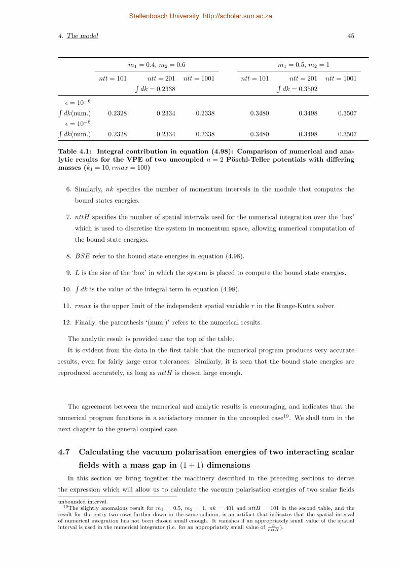
4. The model 45
m1 = 0.4, m2 = 0.6 m1 = 0.5, m2 = 1
ntt = 101 ntt = 201 ntt = 1001 ntt = 101 ntt = 201 ntt = 1001∫dk = 0.2338
∫dk = 0.3502
ε = 10−6
∫dk(num.) 0.2328 0.2334 0.2338 0.3480 0.3498 0.3507
ε = 10−8
∫dk(num.) 0.2328 0.2334 0.2338 0.3480 0.3498 0.3507
Table 4.1: Integral contribution in equation (4.98): Comparison of numerical and ana-lytic results for the VPE of two uncoupled n = 2 Poschl-Teller potentials with differingmasses (k1 = 10, rmax = 100)
6. Similarly, nk specifies the number of momentum intervals in the module that computes the
bound states energies.
7. nttH specifies the number of spatial intervals used for the numerical integration over the ‘box’
which is used to discretise the system in momentum space, allowing numerical computation of
the bound state energies.
8. BSE refer to the bound state energies in equation (4.98).
9. L is the size of the ‘box’ in which the system is placed to compute the bound state energies.
10.∫dk is the value of the integral term in equation (4.98).
11. rmax is the upper limit of the independent spatial variable r in the Runge-Kutta solver.
12. Finally, the parenthesis ‘(num.)’ refers to the numerical results.
The analytic result is provided near the top of the table.
It is evident from the data in the first table that the numerical program produces very accurate
results, even for fairly large error tolerances. Similarly, it is seen that the bound state energies are
reproduced accurately, as long as nttH is chosen large enough.
The agreement between the numerical and analytic results is encouraging, and indicates that the
numerical program functions in a satisfactory manner in the uncoupled case19. We shall turn in the
next chapter to the general coupled case.
4.7 Calculating the vacuum polarisation energies of two interacting scalar
fields with a mass gap in (1 + 1) dimensions
In this section we bring together the machinery described in the preceding sections to derive
the expression which will allow us to calculate the vacuum polarisation energies of two scalar fields
unbounded interval.19The slightly anomalous result for m1 = 0.5, m2 = 1, nk = 401 and nttH = 101 in the second table, and the
result for the entry two rows further down in the same column, is an artifact that indicates that the spatial intervalof numerical integration has not been chosen small enough. It vanishes if an appropriately small value of the spatialinterval is used in the numerical integrator (i.e. for an appropriately small value of L
nttH).
Stellenbosch University http://scholar.sun.ac.za

4. The model 46
m1 = 0.4, m2 = 0.6
nttH = 101 nttH = 201 nttH = 1001
BSE = −0.5669
nk = 201
BSE(num.) -0.5524 -0.5626 -0.5669
nk = 401
BSE(num.) -0.5495 -0.5595 -0.5669
nk = 801
BSE(num.) -0.5484 -0.5579 -0.5668
Table 4.2: Bound state contribution in equation (4.98): Comparison of numerical andanalytic results for the VPE of two uncoupled n = 2 Poschl-Teller potentials(m1 = 0.4,m2 = 0.6 and L = 60)
m1 = 0.5, m2 = 1
nttH = 101 nttH = 201 nttH = 1001
BSE = −0.8504
nk = 201
BSE(num.) -0.8296 -0.8439 -0.8504
nk = 401
BSE(num.) -0.6995 -0.8394 -0.8504
nk = 801
BSE(num.) -0.6890 -0.8373 -0.8502
Table 4.3: Bound state contribution in equation (4.98): Comparison of numerical andanalytic results for the VPE of two uncoupled n = 2 Poschl-Teller potentials(m1 = 0.5,m2 = 1 and L = 60)
of given masses interacting via a radially symmetric potential that is assumed to be regular as in
equation (2.10)20. In strict analogy with the example in section 2.4 we write the energy difference
between the free and interacting cases as a sum over a finite number of bound states and an integral
weighted by a factor that is essentially the difference between the density of states in the free and
interacting cases. The lower integration bound is now E = m1, which corresponds to k1 = 0 in the
first channel. The relevant equation is then
∆E =1
2
b.s.∑
j
(ωj −m1) +1
2πi
∫ ∞
m1
dE(E −m1)d
dE[ln detS(E)]N +
N∑
i=1
E(i)FD + ECT . (4.102)
It is understood that the subscript N means that that factor is already Born subtracted (to order N),
and the ωj are the binding energies of section 4.5. The factor of (E −m1) in the integrand ensures
that the integral exists: the Born approximation goes like 1k , so without this factor the integrand
would diverge at small k1 (or for E near m1).
20We shall find an additional bound for the exponential potential, as we shall see in a later section.
Stellenbosch University http://scholar.sun.ac.za
4. The model 47
Integration by parts on the second term yields
1
2πi
∫ ∞
m1
dE(E −m1)d
dE[ln detS(E)]N =
1
2i(E −m1)[ln detS(E)]N |∞m1
− 1
2i
∫ ∞
m1
dE[ln detS(E)]N
=1
2πi[(∞−m1)[ln detS(∞)]N ]− 1
2πi
∫ ∞
m1
dE[ln detS(E)]N
= −∑
p=+1,−1
∫ ∞
m1
dE
π[δp(E)− δ(1)
p (E)]. (4.103)
Here the fact that the S-matrix goes to unity at large momenta was used in the last line. Note also that
from equation (4.69) it follows that∑
j
δj(E) = 2i ln detS(E). The sum over p refers to the parity,
i.e. δ(E) is already the sum of the phase shifts and the summation sign refers to the summation over
the symmetric and antisymmetric channels.
Combining this with the previous equation, the quantity of interest is
∆E =1
2
b.s.∑
j
(ωj −m1)−∑
p=+1,−1
∫ ∞
m1
dE
π[δp(E)− δ(1)
p (E)] +N∑
i=1
E(i)FD + ECT . (4.104)
It should be clear at this point how the actual calculation of the VPE in (1 + 1) dimensions is to
proceed: For two masses, m1 6= m2, and a potential that is Hermitian, radial and regular, we calculate
the sum of the phase shifts and the Born approximations thereof numerically by solving equations
(4.69), (4.83), and the relevant equations for the symmetric channel, on a computer. This then allows
the integral in the expression above to be calculated numerically, and this quantity is then added to
the sum over the bound states, which are also computed numerically as described in section 4.5.
Stellenbosch University http://scholar.sun.ac.za
5 Numerical Analysis
All the machinery required to calculate the VPE has been been assembled. In this chapter we bring
all of this together to give the numerical results for a number of potentials with varying parameters, as
well as general comments on the analyticity of the Jost function and some further comments on how
the numerical data were computed. See the appendices for details of the relevant numerical methods.
5.1 Comments on the numerical aspect of the problem
Analyticity (in the sense of the satisfaction of the Cauchy-Riemann equations and the absence of
singularities) of the generalised Jost function is essential for the success of the spectral method. This
can be checked numerically by comparing the integrals associated with the VPE along the real and
positive imaginary momentum axes. If the Jost function is analytic, then the integral must have the
same value along both axes. If the function is not analytic, we must reconsider our assumptions and
find the reason for the non-analyticity by reexamining the analytic structure with respect to poles
and branch cuts. However, before we can make statements about the analyticity it is important that
we deal appropriately with the various numerical issues that already occur along the real axis.
The starting point is the integral appearing in equation (4.104). Due to the (integrable) singularities
appearing near threshold (i.e. at E = m1), it is convenient to reparameterise it as a function of the
momentum k1. We do so, perform some integration ‘tricks’, and identify the sum of the phase shifts
as the trace of the logarithm of the generalised Jost function. Doing so, we have
I = −∑
p=+1,−1
∫ ∞
0
dk1
π
k1√k1
2 +m21
[δp(k1)− δ(1)p (k1)]
= − 1
2πi
∫ ∞
0
dk1k1√
k12 +m2
1
tr[lnF (−k1)− lnF (k1)]1
= − 1
2πi
∫ ∞
−∞dk1
k1√k1
2 +m21
tr[lnF (k1)]1
= − 1
2πi
∫ ∞
−∞dk1
√k1
2 +m21
d
dk1tr[lnF (k1)]1. (5.1)
It is understood that the subscript in tr[lnF ]1 implies that the first Born term has been subtracted
from the expression.
We now have an integral along the whole real k1 axis. We can relate this to the contour integral
of the analytic continuation of the relevant function along the path illustrated in diagram 4.1 by the
judicious use of Cauchy’s theorem21. The poles corresponding to bound states on the imaginary axis
21See appendix A for a derivation of Levinson’s theorem for s-wave which follows the same general procedure as thiscalculation.
48
Stellenbosch University http://scholar.sun.ac.za

5. Numerical Analysis 49
cancel the contribution from the sum in (4.104). We are left with the following integral along the
imaginary axis from the cut at k1 = im1 in the parameter t = −ik1:
∆E = −∫ ∞
m1
dt
2π
√t2 −m2
1
d
dttr lnF (it) +
N∑
i=1
E(i)FD + ECT
= −∫ ∞
m1
dt
2π
t√t2 −m2
1
tr lnF (it) +N∑
i=1
E(i)FD + ECT . (5.2)
This should be compared to equation (4.52), which was derived in the context of QFT without explicit
reference to phase shifts or a Jost-like function. This leads to the identification
d
dttr[lnF (it)]N =
∫ ∞
0
dr[ρ(t, r)]N , (5.3)
which allows us to make contact between the numerical (LHS) and formal QFT (RHS) formalisms.
Without this identification our approach would be ambiguous. It is clear that for our approach to be
applicable the expression above for ∆E must be equal to (4.104) (or the equivalent expression in the
k1 parameterisation).
5.1.1 Singularities at small momenta
It is in practice convenient to calculate the relevant integrals in the k1 parameterisation. This is
because of the behaviour of the integrand near the threshold. This is clear if we consider the analytic
expressions for the first Born approximation (which are known, in contrast to the exact phase shift).
In n = 1 spatial dimension and one channel, for an arbitrary radial potential, they are given in the
symmetric and antisymmetric channels respectively by [3]
δ(1)S (k) = −1
k
∫ ∞
0
drV (r) cos2(kr)
δ(1)A (k) = −1
k
∫ ∞
0
drV (r) sin2(kr). (5.4)
This gives us some insight into what to expect in the two channel case. Specifically, if we compute
the integrand in the E parameterisation we expect to find two (integrable) singularities in the even
channel, one at E = m1, because of the 1k1
behaviour there, and the other at E = m2. However, in
the k1 parameterisation the factor of k1 cancels the first singularity, and the other one is shifted to
k1 = ∆m =√m2
2 −m21 . The latter is an integrable square root singularity in the E parameterisation,
but still requires special treatment numerically. We do so as follows: If we denote the integrand by
g(k1), then the preceding comments on the behaviour for small momenta is equivalent to expecting
g(k1)|k1∼∆m =Ck1√
k21 −∆m2
, (5.5)
Stellenbosch University http://scholar.sun.ac.za

5. Numerical Analysis 50
where C is some appropriate numerical constant. Then we may perform the integration over k1 near
the mass gap by
∫ ∆m+δk1
∆m
dk1g(k1) =
∫ ∆m+δk1
∆m
dk1Ck1√
k21 −∆m2
≈ C∆m
∫ δk1
0
dq1√
2q∆m
= C√
2∆mδk1 , (5.6)
where δk1 is the size of the momentum interval in the numerical program. If this ansatz for the
behaviour of g(k1)|k1∼∆m is correct, then we may extract C from the numerical data by
C = limk1→∆m
g(k1)√k2
1 −∆m2
k1. (5.7)
In practice, the numerical parameters need to be tweaked to make sure that the integral does not have
a dependence on the upper momentum limit. If this is not an issue we can perform the numerical
integration from k1 = ∆m to k1 = ∆m+δk1 using this method. This is implicitly the case for the rest
of the discussion in this chapter. Note also that this issue does not occur at all in the odd channel.
5.1.2 Numerical integration over unbounded intervals
The integral which gives the expression for the VPE must be computed numerically over an un-
bounded interval. It is clearly not possible to calculate an infinite number of points on a computer.
However, the following trick allows us to get around this limitation. Let us consider some integral
I =
∫ ∞
a
dk1g(k1). (5.8)
If it so happens that there exists a number k1 such that ∀k1 ≥ k1 the function g(k1) ≈ Dkn1
, where D
is an appropriate constant and n an integer, then
I =
∫ k1
a
dk1g(k1) +
∫ ∞
k1
dk1D
kn1
=
∫ k1
a
dk1g(k1) +D
(n− 1)kn−11
=
∫ k1
a
dk1g(k1) +k1
n− 1g(k1). (5.9)
It is fortunately known [18] that our integrand is of O(1/k31) on the real axis, and of O(1/k2
1) on the
imaginary axis, so we can make use of this method to integrate over the unbounded interval. We must
however be sure to choose a large enough numerical upper bound on the integral. We can check this
by varying the upper parameter k1. It is implicitly the case for all the results that follow that this
parameter was chosen suitably large.
Stellenbosch University http://scholar.sun.ac.za

5. Numerical Analysis 51
5.1.3 Summary of the approach to performing the numerical integration
It is convenient to summarise the previous discussion regarding the numerical integration. The
figure below breaks the integral on the real axis into a number of intervals. The dependent variable
is the integrand g(k1) ≡ k1E
∑p=+1,−1[δp(k1)− δ(1)
p (k1)]. Considering them one by one, with reference
to figure 5.1:
1∫∆m−εε
dk1g(k1); in this case we can compute and tabulate g(k1) numerically, and then integrate
using the numerical method discussed in appendix B.
2∫∆m
∆m−ε dk1g(k1); if ε is taken small enough we can simply ignore this piece.
3∫∆m+δk1
∆mdk1g(k1); we make the ansatz as in section 5.1.1 and get the contribution C
√2∆mδk1 .
4 22∫ k1max
∆m+δk1dk1g(k1); in this case we can compute and tabulate g(k1) numerically, and then
integrate using the numerical method discussed in appendix B.
5∫∞k1max
dk1g(k1); the integration over the unbounded interval is performed as in equation (5.9).
∆m
∆m− ε ∆m+ δk1
k1maxε
g(k1) = k1E f(k1)
k1
1 3
2 4
5
Figure 5.1: The various integration intervals involved in the computation of ∆E on the real axis. The plot
itself is just for illustration of the general behaviour of the integrand in the even channel.
22Number four only occurs in the even channel, as has been discussed previously.
Stellenbosch University http://scholar.sun.ac.za
5. Numerical Analysis 52
5.1.4 A note on the numerical instability of the exponential potential in (1+1) dimen-
sions, and the continuity of the S-matrix
There are certain technical difficulties associated with investigating the exponential potential ∝e−µr. Specifically, an imprudent choice of the parameter µ leads to a strong dependence of the solution
of the DEQs on the maximum value of the independent variable r in the numerical integrator. This is
evident from the equations in section 4.4 if we introduce the notation V = (Vij)e−µr for the potential
matrix, where the subscripts label the entries of that matrix. The second derivative of the second
field is then
φ′′2(r) = (∆m2 − k21)φ2 + e−µr(V21φ1 + V22φ2), (5.10)
where ∆m =√m2
2 −m21 . We want the potential to disappear at spatial infinity, so that the two
fields decouple and φ2 ∼ (∆m2 − k21)φ2. In the gap the lighter and heavier fields go respectively like
φ1 ∼ eik1r and φ2 ∼ e−κr (where κ =√
∆m2 − k21 ) as r → ∞, i.e. the heavier field is exponentially
damped. Substituting this in the expression above we then have
κ2 = (∆m2 − k21) + V21e
(κ−µ)reik1r, (5.11)
which describes the large r behaviour. Note that the term like V22φ2 has been omitted because it
includes a factor e−µr which suppresses it as r →∞.
Clearly, if κ > µ, then the dominant term on the right hand side of this equation is the second
one, rather than the first one, which is required if the equation is to satisfy the boundary condition
limr→∞
F = I2. The simplest resolution of this problem is simply to restrict our investigation to values
of the parameter µ > ∆m.
In fact, the issue is with the assumption of regular potentials. If we make the more restrictive
choice, that our potential must satisfy
∫ ∞
0
drV (r)e√m2
2−m21 r <∞, (5.12)
then the numerical instability does not occur. The reader can verify that if one chooses an exponential
potential this integral diverges for ∆m > µ, and converges otherwise. So for the case of two scalar
fields with a mass gap coupled by a exponential potential we find that it is the size of the mass gap ∆m
relative to the magnitude of the coupling µ that determines whether the solution has the appropriate
asymptotic behaviour.
Stated differently, if the the parameter µ is not suitably restricted then we would have to change
the ansatz (4.66) to something like
A =
e−ik1r 0
0 e−µr
, (5.13)
and the fields would not decouple to two plane waves: There would be a field decaying exponentially
(i.e. something like a bound state), with this decay dependent not on the momentum but on the
parameter µ. The other channel would, however, still be scattering.
Because the simplest way to increase the number of bound states is to decrease the size of the
Stellenbosch University http://scholar.sun.ac.za

5. Numerical Analysis 53
parameter µ, this result has serious consequences for any attempt verify Levinson’s theorem for two
coupled fields. We shall see that while Levinson’s theorem holds for potentials that allow one bound
state, we cannot speak with certainty for potentials that allow more, precisely because of this restric-
tion. This is not, however, a fundamental limitation, as we can adapt the differential equations as in
the preceding discussion to take the necessary boundary conditions into consideration.
The discussion in this section is summarised by the following figures, which show the dependence
of the phase shifts on the upper limit of the independent variable rmax if the parameter µ is chosen
improperly/properly for an exponential potential. Plots for a Gaussian potential are also included.
The exponential potential corresponds to potential P4 in appendix C, while the Gaussian potential
corresponds to P5. Explicitly, figures 5.2 and 5.4 have unacceptable values of µ, while the rest are
acceptable, in the sense that they do not depend on rmax. Some comments on the continuity of the
S-matrix follow the figures.
0
2
4
6
8
10
12
14
0 1 2 3 4 5 6 7 8 9 10 11
Phase
shifts
E
Even channel
0
2
4
6
8
10
12
14
0 1 2 3 4 5 6 7 8 9 10 11
Phase
shifts
E
Even channel
-2
0
2
4
6
8
10
12
14
0 1 2 3 4 5 6 7 8 9 10 11
Phase
shifts
E
Even channel
0
2
4
6
8
10
12
14
0 1 2 3 4 5 6 7 8 9 10 11
Phase
shifts
E
Even channel
Figure 5.2: Behaviour of phase shifts for the exponential potential P4 if µ < ∆m. Clock-
wise from top left: rmax = 10, 20, 30, 40 (even channel, m1 = 0.5, m2 = 1, µ = 0.4).
Stellenbosch University http://scholar.sun.ac.za
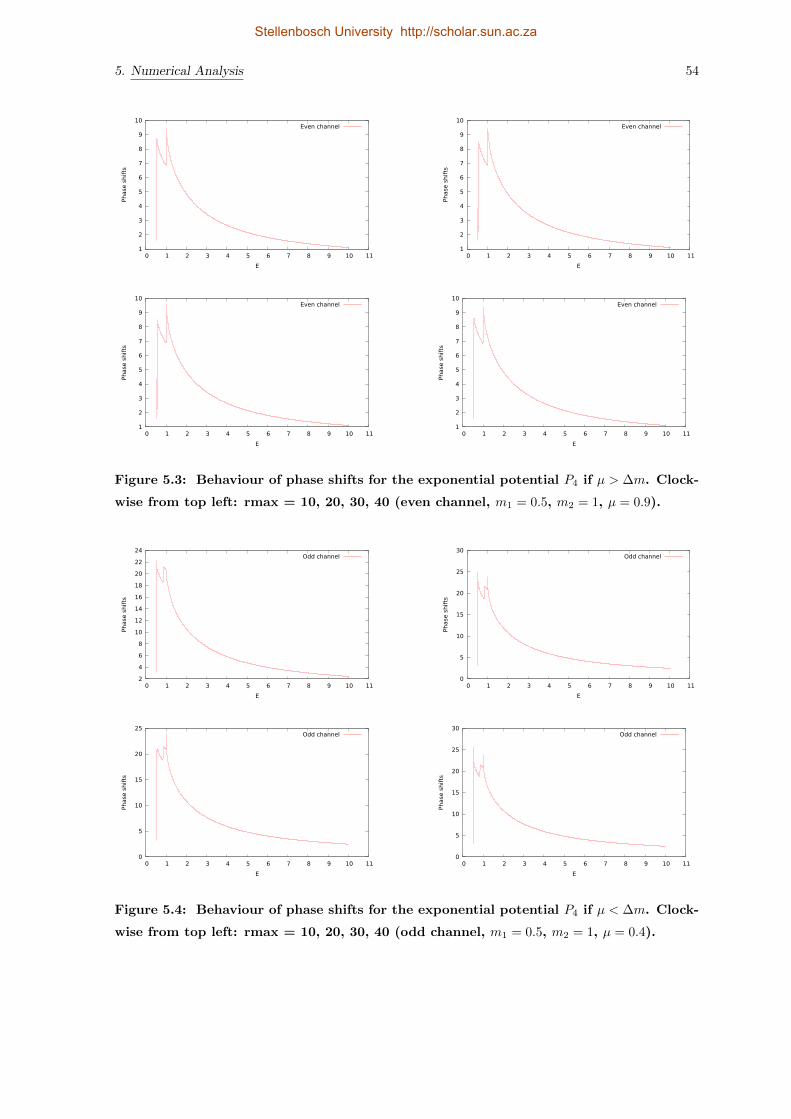
5. Numerical Analysis 54
1
2
3
4
5
6
7
8
9
10
0 1 2 3 4 5 6 7 8 9 10 11
Phase
shifts
E
Even channel
1
2
3
4
5
6
7
8
9
10
0 1 2 3 4 5 6 7 8 9 10 11
Phase
shifts
E
Even channel
1
2
3
4
5
6
7
8
9
10
0 1 2 3 4 5 6 7 8 9 10 11
Phase
shifts
E
Even channel
1
2
3
4
5
6
7
8
9
10
0 1 2 3 4 5 6 7 8 9 10 11Phase
shifts
E
Even channel
Figure 5.3: Behaviour of phase shifts for the exponential potential P4 if µ > ∆m. Clock-
wise from top left: rmax = 10, 20, 30, 40 (even channel, m1 = 0.5, m2 = 1, µ = 0.9).
2
4
6
8
10
12
14
16
18
20
22
24
0 1 2 3 4 5 6 7 8 9 10 11
Phase
shifts
E
Odd channel
0
5
10
15
20
25
30
0 1 2 3 4 5 6 7 8 9 10 11
Phase
shifts
E
Odd channel
0
5
10
15
20
25
0 1 2 3 4 5 6 7 8 9 10 11
Phase
shifts
E
Odd channel
0
5
10
15
20
25
30
0 1 2 3 4 5 6 7 8 9 10 11
Phase
shifts
E
Odd channel
Figure 5.4: Behaviour of phase shifts for the exponential potential P4 if µ < ∆m. Clock-
wise from top left: rmax = 10, 20, 30, 40 (odd channel, m1 = 0.5, m2 = 1, µ = 0.4).
Stellenbosch University http://scholar.sun.ac.za
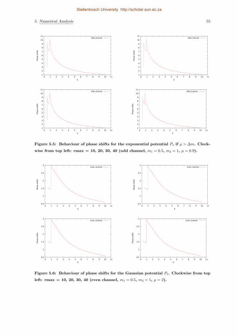
5. Numerical Analysis 55
1
2
3
4
5
6
7
8
9
10
11
0 1 2 3 4 5 6 7 8 9 10 11
Phase
shifts
E
Odd channel
1
2
3
4
5
6
7
8
9
10
11
0 1 2 3 4 5 6 7 8 9 10 11
Phase
shifts
E
Odd channel
1
2
3
4
5
6
7
8
9
10
11
0 1 2 3 4 5 6 7 8 9 10 11
Phase
shifts
E
Odd channel
1
2
3
4
5
6
7
8
9
10
11
0 1 2 3 4 5 6 7 8 9 10 11Phase
shifts
E
Odd channel
Figure 5.5: Behaviour of phase shifts for the exponential potential P4 if µ > ∆m. Clock-
wise from top left: rmax = 10, 20, 30, 40 (odd channel, m1 = 0.5, m2 = 1, µ = 0.9).
0.5
1
1.5
2
2.5
3
0 1 2 3 4 5 6 7 8 9 10 11
Phase
shifts
E
Even channel
0.5
1
1.5
2
2.5
3
0 1 2 3 4 5 6 7 8 9 10 11
Phase
shifts
E
Even channel
0.5
1
1.5
2
2.5
3
0 1 2 3 4 5 6 7 8 9 10 11
Phase
shifts
E
Even channel
0.5
1
1.5
2
2.5
3
0 1 2 3 4 5 6 7 8 9 10 11
Phase
shifts
E
Even channel
Figure 5.6: Behaviour of phase shifts for the Gaussian potential P5. Clockwise from top
left: rmax = 10, 20, 30, 40 (even channel, m1 = 0.5, m2 = 1, µ = 2).
Stellenbosch University http://scholar.sun.ac.za
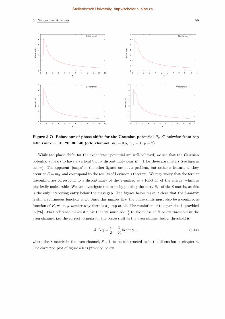
5. Numerical Analysis 56
0
1
2
3
4
5
6
7
0 1 2 3 4 5 6 7 8 9 10 11
Phase
shifts
E
Odd channel
0
1
2
3
4
5
6
7
0 1 2 3 4 5 6 7 8 9 10 11
Phase
shifts
E
Odd channel
0
1
2
3
4
5
6
7
0 1 2 3 4 5 6 7 8 9 10 11
Phase
shifts
E
Odd channel
0
1
2
3
4
5
6
7
0 1 2 3 4 5 6 7 8 9 10 11Phase
shifts
E
Odd channel
Figure 5.7: Behaviour of phase shifts for the Gaussian potential P5. Clockwise from top
left: rmax = 10, 20, 30, 40 (odd channel, m1 = 0.5, m2 = 1, µ = 2).
While the phase shifts for the exponential potential are well-behaved, we see that the Gaussian
potential appears to have a vertical ‘jump’ discontinuity near E = 1 for these parameters (see figures
below). The apparent ‘jumps’ in the other figures are not a problem, but rather a feature, as they
occur at E = m2, and correspond to the results of Levinson’s theorem. We may worry that the former
discontinuities correspond to a discontinuity of the S-matrix as a function of the energy, which is
physically undesirable. We can investigate this issue by plotting the entry S11 of the S-matrix, as this
is the only interesting entry below the mass gap. The figures below make it clear that the S-matrix
is still a continuous function of E. Since this implies that the phase shifts must also be a continuous
function of E, we may wonder why there is a jump at all. The resolution of this paradox is provided
in [26]. That reference makes it clear that we must add π2 to the phase shift below threshold in the
even channel, i.e. the correct formula for the phase shift in the even channel below threshold is
δ+(E) =π
2+
1
2iln detS+, (5.14)
where the S-matrix in the even channel, S+, is to be constructed as in the discussion in chapter 4.
The corrected plot of figure 5.6 is provided below.
Stellenbosch University http://scholar.sun.ac.za
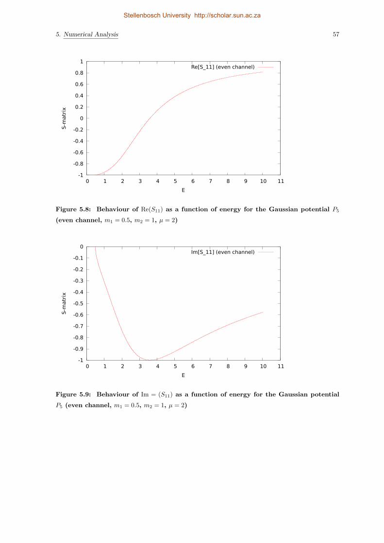
5. Numerical Analysis 57
-1
-0.8
-0.6
-0.4
-0.2
0
0.2
0.4
0.6
0.8
1
0 1 2 3 4 5 6 7 8 9 10 11
S-m
atr
ix
E
Re[S_11] (even channel)
Figure 5.8: Behaviour of Re(S11) as a function of energy for the Gaussian potential P5
(even channel, m1 = 0.5, m2 = 1, µ = 2)
-1
-0.9
-0.8
-0.7
-0.6
-0.5
-0.4
-0.3
-0.2
-0.1
0
0 1 2 3 4 5 6 7 8 9 10 11
S-m
atr
ix
E
Im[S_11] (even channel)
Figure 5.9: Behaviour of Im = (S11) as a function of energy for the Gaussian potential
P5 (even channel, m1 = 0.5, m2 = 1, µ = 2)
Stellenbosch University http://scholar.sun.ac.za

5. Numerical Analysis 58
0.5
1
1.5
2
2.5
3
3.5
0 1 2 3 4 5 6 7 8 9 10 11
Phase
shifts
E
Even channel
Figure 5.10: Corrected behaviour of phase shifts for the Gaussian potential P5 (even
channel, m1 = 0.5, m2 = 1, µ = 2, rmax = 10)
5.2 Numerical results along the real momentum axis
In this section the results (up to four decimal places) of the numerical calculations along the real
momentum axis for a specific potential with different parameters (i.e. both model and Runge-Kutta
parameters) are presented for the coupled case. If we are to trust our results we require them to
be numerically stable, in the sense that they must ‘settle down’ to a fixed value when the numerical
parameters are chosen appropriately. The data are presented in several tables, as in the example of
the uncoupled potentials that was performed as a consistency check (see section 4.6 for a reminder
of the importance of the various parameters). We must also carefully consider the behaviour of the
various pieces of the integral as outlined in subsection 5.1.3.
We consider the potential
V (r) = −e−µr
0.6 0.4
0.4 0.6
, (5.15)
which corresponds to P3 in appendix C. We could have included any number of other potentials; this
one was chosen merely by way of convenience. All the other potentials investigated with the numerical
program showed comparable properties with respect to stability of the integral for different numerical
parameters, so endless tables of numerical data would give us no more insight into the problem in this
thesis. We are not interested in any specific potential, only whether the spectral method is applicable.
To that end it is sufficient to establish that the numerical data is well-behaved, which appears to be
the case.
The VPE is calculated from equation (4.104), with the numerical piece reproduced here for con-
venience in the k1 parameterisation:
∆Enumerical =1
2
b.s.∑
j
(ωj −m1)− 1
π
∑
p=+1,−1
∫ ∞
0
dk1k1√
k21 +m2
1
[δp(k1)− δ(1)p (k1)]. (5.16)
Stellenbosch University http://scholar.sun.ac.za
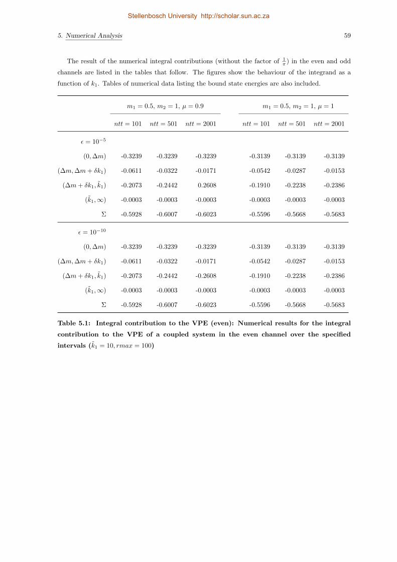
5. Numerical Analysis 59
The result of the numerical integral contributions (without the factor of 1π ) in the even and odd
channels are listed in the tables that follow. The figures show the behaviour of the integrand as a
function of k1. Tables of numerical data listing the bound state energies are also included.
m1 = 0.5, m2 = 1, µ = 0.9 m1 = 0.5, m2 = 1, µ = 1
ntt = 101 ntt = 501 ntt = 2001 ntt = 101 ntt = 501 ntt = 2001
ε = 10−5
(0,∆m) -0.3239 -0.3239 -0.3239 -0.3139 -0.3139 -0.3139
(∆m,∆m+ δk1) -0.0611 -0.0322 -0.0171 -0.0542 -0.0287 -0.0153
(∆m+ δk1, k1) -0.2073 -0.2442 0.2608 -0.1910 -0.2238 -0.2386
(k1,∞) -0.0003 -0.0003 -0.0003 -0.0003 -0.0003 -0.0003
Σ -0.5928 -0.6007 -0.6023 -0.5596 -0.5668 -0.5683
ε = 10−10
(0,∆m) -0.3239 -0.3239 -0.3239 -0.3139 -0.3139 -0.3139
(∆m,∆m+ δk1) -0.0611 -0.0322 -0.0171 -0.0542 -0.0287 -0.0153
(∆m+ δk1, k1) -0.2073 -0.2442 -0.2608 -0.1910 -0.2238 -0.2386
(k1,∞) -0.0003 -0.0003 -0.0003 -0.0003 -0.0003 -0.0003
Σ -0.5928 -0.6007 -0.6023 -0.5596 -0.5668 -0.5683
Table 5.1: Integral contribution to the VPE (even): Numerical results for the integral
contribution to the VPE of a coupled system in the even channel over the specified
intervals (k1 = 10, rmax = 100)
Stellenbosch University http://scholar.sun.ac.za

5. Numerical Analysis 60
m1 = 0.5, m2 = 1, µ = 0.9 m1 = 0.5, m2 = 1, µ = 1
ntt = 101 ntt = 501 ntt = 2001 ntt = 101 ntt = 501 ntt = 2001
ε = 10−5
(0,∆m) 0.0386 0.0386 0.0386 0.0286 0.0285 0.0285
(∆m, k1) -0.0002 0.0006 0.0008 0.0019 0.0026 0.0027
(k1,∞) -0.0003 -0.0003 -0.0003 -0.0003 -0.0003 -0.0003
Σ 0.0380 0.0389 0.0391 0.0302 0.0309 0.0309
ε = 10−10
(0,∆m) 0.0386 0.0386 0.0386 0.0286 0.0285 0.0285
(∆m, k1) -0.0002 0.0006 0.0008 0.0019 0.0026 0.0027
(k1,∞) -0.0003 -0.0003 -0.0003 -0.0003 -0.0003 -0.0003
Σ 0.0380 0.0389 0.0391 0.0302 0.0309 0.0309
Table 5.2: Integral contribution to the VPE (odd): Numerical results for the integral
contribution to the VPE of a coupled system in the odd channel over the specified
intervals (k1 = 10, rmax = 100)
Stellenbosch University http://scholar.sun.ac.za
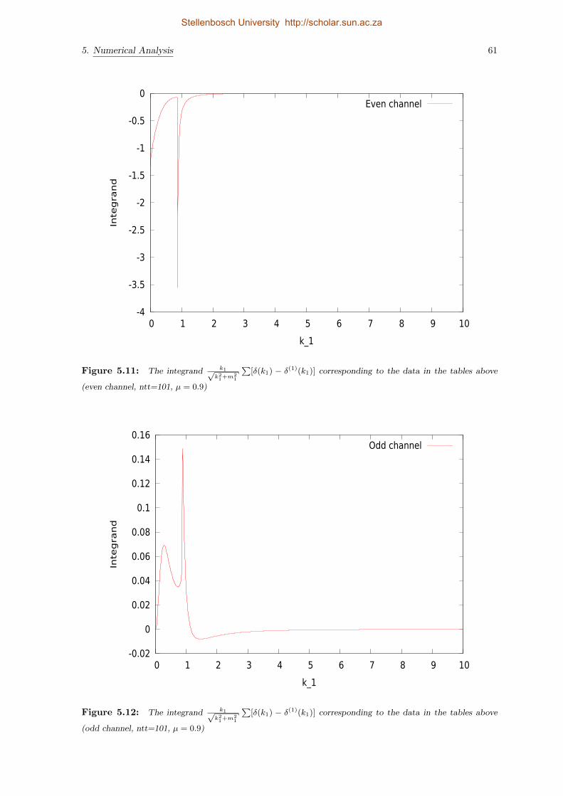
5. Numerical Analysis 61
-4
-3.5
-3
-2.5
-2
-1.5
-1
-0.5
0
0 1 2 3 4 5 6 7 8 9 10
Inte
gra
nd
k_1
Even channel
Figure 5.11: The integrand k1√k21+m
21
∑[δ(k1) − δ(1)(k1)] corresponding to the data in the tables above
(even channel, ntt=101, µ = 0.9)
-0.02
0
0.02
0.04
0.06
0.08
0.1
0.12
0.14
0.16
0 1 2 3 4 5 6 7 8 9 10
Inte
gra
nd
k_1
Odd channel
Figure 5.12: The integrand k1√k21+m
21
∑[δ(k1) − δ(1)(k1)] corresponding to the data in the tables above
(odd channel, ntt=101, µ = 0.9)
Stellenbosch University http://scholar.sun.ac.za
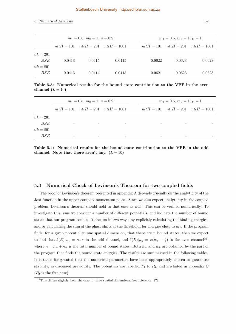
5. Numerical Analysis 62
m1 = 0.5, m2 = 1, µ = 0.9 m1 = 0.5, m2 = 1, µ = 1
nttH = 101 nttH = 201 nttH = 1001 nttH = 101 nttH = 201 nttH = 1001
nk = 201
BSE 0.0413 0.0415 0.0415 0.0622 0.0623 0.0623
nk = 801
BSE 0.0413 0.0414 0.0415 0.0621 0.0623 0.0623
Table 5.3: Numerical results for the bound state contribution to the VPE in the evenchannel (L = 10)
m1 = 0.5, m2 = 1, µ = 0.9 m1 = 0.5, m2 = 1, µ = 1
nttH = 101 nttH = 201 nttH = 1001 nttH = 101 nttH = 201 nttH = 1001
nk = 201
BSE - - - - - -
nk = 801
BSE - - - - - -
Table 5.4: Numerical results for the bound state contribution to the VPE in the oddchannel. Note that there aren’t any. (L = 10)
5.3 Numerical Check of Levinson’s Theorem for two coupled fields
The proof of Levinson’s theorem presented in appendix A depends crucially on the analyticity of the
Jost function in the upper complex momentum plane. Since we also expect analyticity in the coupled
problem, Levinson’s theorem should hold in that case as well. This can be verified numerically. To
investigate this issue we consider a number of different potentials, and indicate the number of bound
states that our program counts. It does so in two ways; by explicitly calculating the binding energies,
and by calculating the sum of the phase shifts at the threshold, for energies close to m1. If the program
finds, for a given potential in one spatial dimension, that there are n bound states, then we expect
to find that δ(E)|m1= n−π in the odd channel, and δ(E)|m1
= π(n+ − 12 ) in the even channel23,
where n = n−+n+ is the total number of bound states. Both n− and n+ are obtained by the part of
the program that finds the bound state energies. The results are summarised in the following tables.
It is taken for granted that the numerical parameters have been appropriately chosen to guarantee
stability, as discussed previously. The potentials are labelled P1 to P6, and are listed in appendix C
(P2 is the free case).
23This differs slightly from the case in three spatial dimensions. See reference [27].
Stellenbosch University http://scholar.sun.ac.za

5. Numerical Analysis 63
m1 = 0.5, m2 = 1, µ = 0.9 m1 = 0.5, m2 = 2, µ = 2.1
P1 P2 P3 P6 P1 P2 P3 P6
n− 0 0 0 0 0 0 0 0
E2 - - - - - - - -
δ(E)|m1 0 0 0 0 0 0 0 0
Table 5.5: Checking Levinson’s theorem for two coupled fields: Counting bound states
(odd channel)
m1 = 0.5, m2 = 1, µ = 0.9 m1 = 0.5, m2 = 2, µ = 2.1
P1 P2 P3 P6 P1 P2 P3 P6
n+ 0 0 1 1 0 0 1 1
E2 - - 0.0415 -0.1464 - - 0.1892 0.9075
δ(E)|m1 -1.5708 0 1.5708 1.5708 -1.5708 0 1.5708 1.5708
Table 5.6: Checking Levinson’s theorem for two coupled fields: Counting bound states
(even channel)
If we specifically consider the results for P1 to P3, we see that this corresponds to the physical
situation of starting with a small repulsive potential, and then gradually tweaking the parameters so
that it goes through zero (V (r) = P2) and then becoming slightly attractive. The resultant phase shifts
correspond to the behaviour expected from [27], which we take to mean that the results correspond
to the correct physical situation.
We conclude that our numerical program counts states in accordance with Levinson’s theorem
in one spatial dimension for potentials P1 to P3, and P6, and that this strongly suggests that the
Jost function is analytic for these potentials. This is essentially a connection between the numerical
scattering data and the topology of the Riemann surface associated with the Jost function. Specifically,
we are counting the number of poles of the surface in figure 4.1.
As stated previously, the restriction on the parameter µ prevents us from investigating potentials
with more than one bound state. This is a technical issue that should be surmountable by further
investigation of the differential equations from which the phase shifts are extracted.
However, the issue is more complicated. For certain potentials it appears that Levinson’s theorem
does not hold. This is the case for potentials with values on the diagonal that are large with respect to
those those on the off-diagonal, as the following table shows. This implies that we must be very careful
when using the methods developed in this thesis to calculate the O(~) corrections to interacting scalar
Stellenbosch University http://scholar.sun.ac.za

5. Numerical Analysis 64
fields, as they may not be applicable to certain potentials. This is an issue that warrants further
attention, but we are in general satisfied with the robustness and validity of this approach, as long as
this issue is taken into consideration.
m1 = 0.5, m2 = 1, µ = 0.9 m1 = 0.5, m2 = 2, µ = 2.1
P4 P5 P7 P8 P4 P5 P7 P8
n− 1 0 1 1 1 0 0 0
E2 0.0431 - 0.1994 0.1922 0.0651 - - -
δ(E)|m1 3.1416 3.1417 3.1418 3.1419 3.1414 3.1413 0 0
Table 5.7: Investigating the failure of Levinson’s theorem for certain potentials : Count-
ing bound states (odd channel)
m1 = 0.5, m2 = 1, µ = 0.9 m1 = 0.5, m2 = 2, µ = 2.1
P4 P5 P7 P8 P4 P5 P7 P8
n+ 0 1 0 0 0 0 1 1
E2 - 0.0269 - - - - -0.1904 -0.1986
δ(E)|m1 1.5708 1.5708 1.5708 1.5708 1.5708 1.5708 1.5708 1.5708
Table 5.8: Investigating the failure of Levinson’s theorem for certain potentials : Count-
ing bound states (even channel). Note that the correction from equation (5.14) has not
been included.
Stellenbosch University http://scholar.sun.ac.za

6 Discussion
During the course of this thesis we have seen how tools from potential scattering theory can be
applied to calculate vacuum polarisation energies in the context of Quantum Field Theory. We began
by discussing the properties of the quantum vacuum in a general manner, with several comments
about the Casimir effect and how it may be interpreted to arise from shifts in the zero-point energy
due to the presence of conducting plates.
We then reviewed various results from potential scattering theory. This included the notions of the
regular and Jost solutions, which have their origin in different boundary conditions for the solutions
of the radial Schrodinger equation. The notions of scattering phase shifts, the scattering cross section
and the S-matrix were also introduced, as was the partial wave decomposition. Levinson’s theorem
was introduced as an important tool of the spectral method. The density of states was heuristically
constructed by placing the system in a box of finite length. This notion was extended to the con-
tinuum by considering the difference between the density of states of interacting and free scattering
systems. A simple example was considered to illustrate how all these ideas can be brought together
to determine the vacuum polarisation energy of a scalar field interacting with a static background
field. This required the identification of terms of the Born series with Feynman diagrams, for which a
proof was outlined. This identification makes it clear that the spectral method is only applicable to
renormalisable field theories, and requires the usual counterterms to render the theory finite.
We continued by showing how a certain model describing two interacting fields in the context of
QFT is equivalent to the two channel regular solution from scattering theory. This was achieved by
introducing the kink solution, a soliton that interpolates between the two vacua of one of these fields.
We looked at small fluctuations around this classical solution, and expanded the Lagrangian density
to quadratic order. Some formal manipulations and use of the stationary ansatz then allowed us to
recover the regular solution in two channels. We also established that the regular series in one channel
converges.
Next, we introduced the field theoretic formalism of our toy model that describes two interacting
scalar fields with a mass gap in (1 + 1) dimensions. The system was quantised by the standard ap-
proach of enforcing equal-time commutation relations between the field operator components and the
components of the conjugate momenta in the Heisenberg picture. The Euler-Lagrange equations were
used to obtain the equation of motion. The fields were then expanded in a Fock decomposition, choos-
ing the covariant normalisation and identifying the expansion coefficients as the Jost solutions, rather
than plane waves. The annihilation and creation operators were likewise defined. The commutation
relations for these operators were calculated. We then proceeded to derive the necessary equation for
the energy density, which is the component T00 of the energy momentum tensor.
Following on from this, we extended the scattering theory formalism to describe two fields. A
65
Stellenbosch University http://scholar.sun.ac.za

6. Discussion 66
Green’s function was introduced, and its imaginary part was identified with the local spectral density.
This was then used to rewrite the expression for the energy density obtained previously. This enabled
us to derive an expression for it along the imaginary k1 axis, after appropriate Born subtractions and
evaluation of the integral corresponding to the energy density along a contour in the complex k1 plane.
Starting with a specific ansatz for the form of the scattering wavefunctions, and appropriate bound-
ary conditions, a number of ordinary, second-order complex differential equations were derived. It was
shown how the scattering phase shifts of two scalar fields with a mass gap interacting via a radial
and Hermitian potential can be extracted from these equations. This was done for both the even and
odd channels, and both inside and outside the mass gap. It was also shown how the S-matrix can be
constructed from these equations. A similar analysis was performed to find the differential equations
from which the first Born approximation to the phase shifts could be extracted. It was then explained
how the bound state energies can be determined numerically for a given potential.
The applicability of the numerical method was demonstrated by comparing the numerical results of
our Fortran 90 program to known analytic results for two uncoupled Poschl-Teller potentials. Excellent
agreement was established.
In the next chapter a number of issues related to the numerical integration of the phase shifts were
discussed. The necessary connection between scattering theory and the field theoretic formalism was
made via equation (5.3). An additional restriction on exponential potentials was found if we wish to
make the ansatz inspired by the dispersion relations. We saw that this issue is related to the chosen
boundary conditions, and is thus not a fundamental restriction of the method. Results along the real
k1 axis were presented, and it was established that the relevant integrals are numerically stable.
Finally, we confirmed that the numerical results for the scattering phase shifts of two interacting
scalar fields with a mass gap in one spatial dimension agree with Levinson’s theorem for a number
of potentials. While the numerical confirmation of Levinson’s theorem for these potentials allowing
one bound state strongly suggests that the Jost-like function for two interacting scalar fields with a
mass gap in (1 + 1) dimensions is analytic in those cases, we would ideally like to extend this result
to potentials with more bound states. This issue is currently unresolved, but should in principle only
require another look at the DEQs and further development of the numerical program. An analytic
proof of the analyticity of the Jost function is also desirable, as it is currently outstanding.
A more serious issue is the failure of Levinson’s theorem for certain potentials. This is a problem
that requires further investigation.
The most obvious avenue of further research would be to investigate a similar model in higher
spatial dimensions. While (1 + 1) dimensions presents a useful ‘laboratory’ to investigate effects like
that discussed here, a world with one spatial dimension is not very rich in dynamics, and bears little
resemblance to our own.
It is also conceivable to extend the model by considering more fields, in however many spatial
dimensions. However, the analytic properties of the scattering data quickly become difficult to deal
with when we have more than two fields.
A further hurdle is the dearth of experimentally detected scalar fields, which makes it a difficult
matter to connect the results with experiments in the real world. As the situation stands, the only
fundamental scalar field known to exist in nature (as of early 2014) is the Higgs. The main point
of interest of the toy model considered in this thesis is the treatment of the integrals occurring near
Stellenbosch University http://scholar.sun.ac.za

6. Discussion 67
the mass thresholds, their physical relevance, and whether the Jost function approach of the spectral
method is applicable. The various bosons occurring in the electroweak theory (i.e. the Higgs, W’s
and the Z) also have different masses, so this thesis can be seen as the first small step in applying
spectral methods to more realistic interacting field theories with mass gaps.
Stellenbosch University http://scholar.sun.ac.za

Appendices
68
Stellenbosch University http://scholar.sun.ac.za

69
Appendix A: Proof of Levinson’s Theorem for s-wave
As noted in section 2.3.2 , this section contains a proof of Levinson’s Theorem [19] for s-wave
(l = 0) and regular potentials in three spatial dimensions. We start by considering the following
contour integral along an arbitrary closed path in the complex plane:
∮
C
dzP ′(z)
P (z)=
∮
C
dzd
dzln[P (z)]. (1)
We assume here that P (z) is a polynomial of arbitrary order, P (z) = A(z − z1)(z − z2)...(z − zn),
where the zj are its nondegenerate roots. Then the above becomes
∮
C
dzP ′(z)
P (z)=
∮
C
dz[1
z − z1+
1
z − z2+ ...+
1
z − zn]
= 2πni (2)
where n is the number of roots of P (z) lying inside the contour C, since
1
2πi
∮
C
dz1
(z − a)n=
0 if a is not contained in C
0 if a is contained in C but n 6= 1
1 if a is contained in C and n = 1.
(3)
We can then establish Levinson’s theorem as follows: we consider the contour C0 along the x-axis
from −R to +R that skips the origin with a small semicircle of radius ε above the real axis, plus the
semicircle at R in the upper complex k-plane (see figure 1 below) and evaluate the contour integral of
the derivative of the natural logarithm of the Jost function F (k) along C0 by taking the simultaneous
limits R→∞ and ε→∞. Since we know (property 4 from section 2.3.2 )24 that F (k) is analytic in
the upper k-plane we can use the above to obtain
1
2πi
∮
C0
dkF ′(k)
F (k)= lim
ε→0R→∞
1
2πi[
∫
C1
+
∫
C2
+
∫
C3
+
∫
C4
][dkF ′(k)
F (k)] = n (4)
where n is the number of bound states inside the contour at the binding energies −κ2j . Note that our
construction of C in the figure below allows us to apply Cauchy’s theorem to a multiply connected
domain. Explicitly,
∮
C
dkF ′(k)
F (k)= 0, (5)
so
∮
C0
dkF ′(k)
F (k)=
n∑
j=1
∮
C(iκj ,r)
dkF ′(k)
F (k)= 2πin, (6)
where C(iκj , r) is the circle of some small radius r centered at iκ.
We now use the properties of the Jost function to evaluate the integral along C1 + C2 + C3 + C4
24Further properties in this appendix refer to those occurring in the same section.
Stellenbosch University http://scholar.sun.ac.za

70
C1
C2
C3
C4
iκ1
iκ2
iκn
(−ε, 0)(−R, 0) (+R, 0)
(0, iR)
Cκ1
Cκ2
Cκn
C0 = C1 + C2 + C3 + C4
C = C0 − ∑nj=1Cκj
Figure 1: Integration contour used in the proof of Levinson’s Theorem for the s-wave
term by term.
C1 and C3: From property 2 we have, for real k, F (k) = |F |e−iδ(k), so∫dkF
′(k)F (k) = −i
∫dk d
dk δl(k)
if the integration is along the real axis. Then
1
2πi[
∫
C1
+
∫
C3
][ dkF ′(k)
F (k)] =−i2πi
[
∫ −ε
−R+
∫ +R
+ε
][ dkdδ(k)
dk]
=1
2π[−δ(−ε) + δ(−R)− δ(+R) + δ(+ε)]. (7)
We take the limit as the radius of the semi-circle goes to +∞, to ensure that we enclose all the
bound states, and the limit as the radius of the small semi-circle goes to zero to deal with possible
poles there (i.e. F (0) = 0). We define δ(∞) = 0, which establishes the physically reasonable expec-
tation that a particle incident at infinite energy won’t be perturbed by a regular potential, and is
equivalent to requiring the S-matrix element to go to unity for large k (since δ(k) = 2π implies that
S = I). Then, since δ(−k) = −δ(k) (property 7), the above contributes 1π δ(0) to the total integral
along the contour C, after taking the appropriate limits.
C4: From property 3 we have lim|k|→∞
F ′(k) = 0 so that the semicircle contributes nothing to the
integral.
C2: For the small semicircle we make use of the fact that as k → 0 along the upper complex plane
Stellenbosch University http://scholar.sun.ac.za

71
F (k) = O(k) and F (k)−1 = O(k−1). So
1
2πi
∫
C2
dkF ′(k)
F (k)=
1
2πi
∫ 0
π
dθ = −1
2(8)
if F (0) = 0, and 0 otherwise.
Summing the contributions and rearranging we get Levinson’s theorem in three spatial dimensions,
δ(0) =
nπ if F (0) 6= 0
π(n+ 12 ) if F (0) = 0
(9)
which gives us a remarkably simple relationship between the phase shifts at k = 0 and the number of
bound states for a large class of potentials of type (2.10). The generalisation to l > 0 is
δ(0) = nπ, (10)
which is proved as above without the complication at k = 0.
In one spatial dimension the result in the symmetric channel changes [27] to
δ(0) = π(n− 1
2), (11)
which is relevant to our discussion of the analyticity of the Jost function of two coupled scalar fields
in chapter 5.
Appendix B: Numerical Methods
This appendix contains a concise overview of the various numerical methods and algorithms used
during the course of this thesis, with appropriate references. Unless otherwise stated, all the numer-
ical algorithms were implemented in Fortran 90, after a rather lengthy and unsuccessful attempt at
implementing them in C from scratch25.
Numerical Integration
The numerical integration method used was the 5-point Newton-Cotes formula, also known as
Boole’s rule26. Like all Newton-Cotes formulas, of any order n, Boole’s rule approximates the integral
of a function over an interval by integrating the Legendre interpolating polynomial associated with it.
The Legendre interpolating polynomial of order n is the polynomial which passes through the points
(x1, f(x1)), . . . , (xn, f(xn)), given by
P (x) =n∑
j=1
f(xj)n∏
k=1k 6=j
x− xkxj − xk
. (12)
25This is not recommended.26Due to a misprint in the 1972 edition of Abramowitz and Stegun’s venerable ‘Handbook of Mathematical Functions
with Formulas, Graphs, and Mathematical Tables’ this is widely known as Bode’s Rule.
Stellenbosch University http://scholar.sun.ac.za
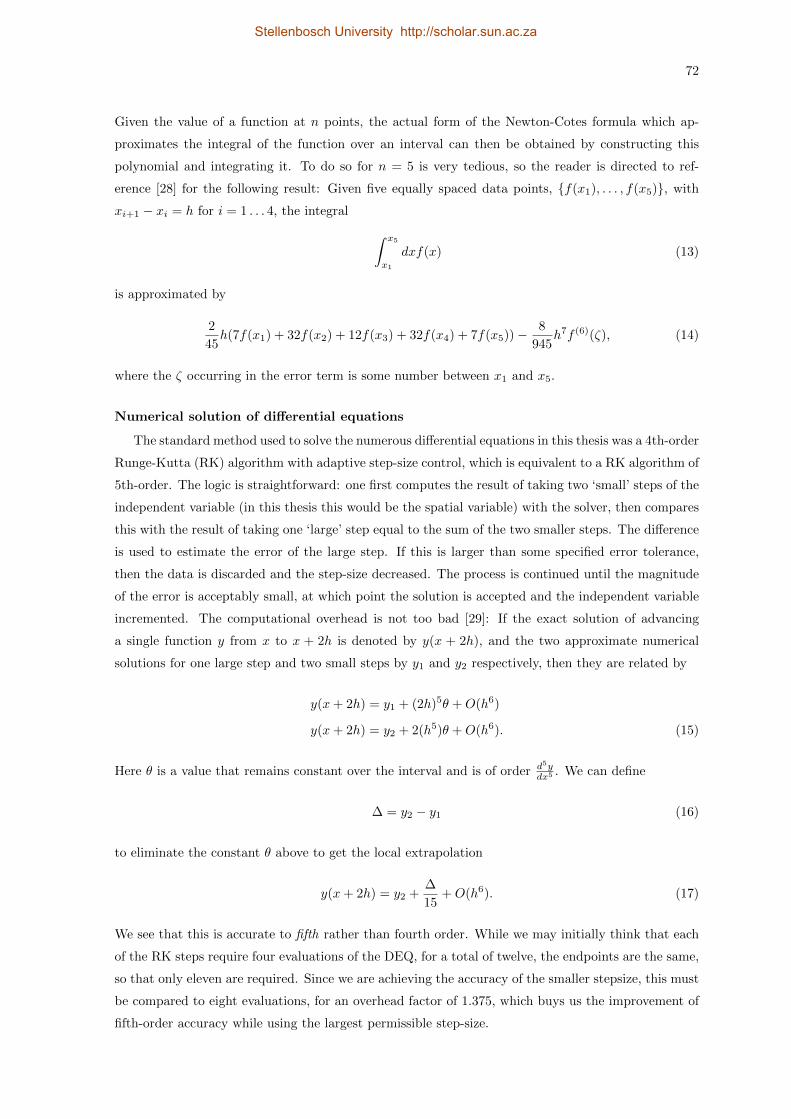
72
Given the value of a function at n points, the actual form of the Newton-Cotes formula which ap-
proximates the integral of the function over an interval can then be obtained by constructing this
polynomial and integrating it. To do so for n = 5 is very tedious, so the reader is directed to ref-
erence [28] for the following result: Given five equally spaced data points, f(x1), . . . , f(x5), with
xi+1 − xi = h for i = 1 . . . 4, the integral
∫ x5
x1
dxf(x) (13)
is approximated by
2
45h(7f(x1) + 32f(x2) + 12f(x3) + 32f(x4) + 7f(x5))− 8
945h7f (6)(ζ), (14)
where the ζ occurring in the error term is some number between x1 and x5.
Numerical solution of differential equations
The standard method used to solve the numerous differential equations in this thesis was a 4th-order
Runge-Kutta (RK) algorithm with adaptive step-size control, which is equivalent to a RK algorithm of
5th-order. The logic is straightforward: one first computes the result of taking two ‘small’ steps of the
independent variable (in this thesis this would be the spatial variable) with the solver, then compares
this with the result of taking one ‘large’ step equal to the sum of the two smaller steps. The difference
is used to estimate the error of the large step. If this is larger than some specified error tolerance,
then the data is discarded and the step-size decreased. The process is continued until the magnitude
of the error is acceptably small, at which point the solution is accepted and the independent variable
incremented. The computational overhead is not too bad [29]: If the exact solution of advancing
a single function y from x to x + 2h is denoted by y(x + 2h), and the two approximate numerical
solutions for one large step and two small steps by y1 and y2 respectively, then they are related by
y(x+ 2h) = y1 + (2h)5θ +O(h6)
y(x+ 2h) = y2 + 2(h5)θ +O(h6). (15)
Here θ is a value that remains constant over the interval and is of order d5ydx5 . We can define
∆ = y2 − y1 (16)
to eliminate the constant θ above to get the local extrapolation
y(x+ 2h) = y2 +∆
15+O(h6). (17)
We see that this is accurate to fifth rather than fourth order. While we may initially think that each
of the RK steps require four evaluations of the DEQ, for a total of twelve, the endpoints are the same,
so that only eleven are required. Since we are achieving the accuracy of the smaller stepsize, this must
be compared to eight evaluations, for an overhead factor of 1.375, which buys us the improvement of
fifth-order accuracy while using the largest permissible step-size.
Stellenbosch University http://scholar.sun.ac.za
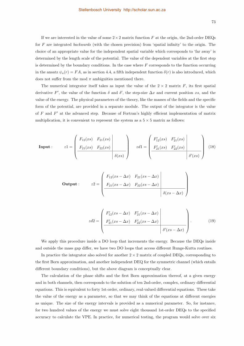
73
If we are interested in the value of some 2×2 matrix function F at the origin, the 2nd-order DEQs
for F are integrated backwards (with the chosen precision) from ‘spatial infinity’ to the origin. The
choice of an appropriate value for the independent spatial variable which corresponds to ‘far away’ is
determined by the length scale of the potential. The value of the dependent variables at the first step
is determined by the boundary conditions. In the case where F corresponds to the function occurring
in the ansatz ψa(r) = FA, as in section 4.4, a fifth independent function δ(r) is also introduced, which
does not suffer from the mod π ambiguities mentioned there.
The numerical integrator itself takes as input the value of the 2 × 2 matrix F , its first spatial
derivative F ′, the value of the function δ and δ′, the step-size ∆x and current position xs, and the
value of the energy. The physical parameters of the theory, like the masses of the fields and the specific
form of the potential, are provided in a separate module. The output of the integrator is the value
of F and F ′ at the advanced step. Because of Fortran’s highly efficient implementation of matrix
multiplication, it is convenient to represent the system as a 5× 5 matrix as follows:
Input : z1 =
F12(xs) F21(xs)
F21(xs) F22(xs)
δ(xs)
zd1 =
F ′12(xs) F ′21(xs)
F ′21(xs) F ′22(xs)
δ′(xs)
(18)
Output : z2 =
F12(xs−∆x) F21(xs−∆x)
F21(xs−∆x) F22(xs−∆x)
δ(xs−∆x)
zd2 =
F ′12(xs−∆x) F ′21(xs−∆x)
F ′21(xs−∆x) F ′22(xs−∆x)
δ′(xs−∆x)
. (19)
We apply this procedure inside a DO loop that increments the energy. Because the DEQs inside
and outside the mass gap differ, we have two DO loops that access different Runge-Kutta routines.
In practice the integrator also solved for another 2× 2 matrix of coupled DEQs, corresponding to
the first Born approximation, and another independent DEQ for the symmetric channel (which entails
different boundary conditions), but the above diagram is conceptually clear.
The calculation of the phase shifts and the first Born approximation thereof, at a given energy
and in both channels, then corresponds to the solution of ten 2nd-order, complex, ordinary differential
equations. This is equivalent to forty 1st-order, ordinary, real-valued differential equations. These take
the value of the energy as a parameter, so that we may think of the equations at different energies
as unique. The size of the energy intervals is provided as a numerical parameter. So, for instance,
for two hundred values of the energy we must solve eight thousand 1st-order DEQs to the specified
accuracy to calculate the VPE. In practice, for numerical testing, the program would solve over six
Stellenbosch University http://scholar.sun.ac.za

74
million equations in one run.
Numerical checks on the differential solver
The program used to solve the DEQs occurring in this thesis is complex enough that we need
some way of checking that the output is sensible. There are many ways in which errors can enter into
the solution of the DEQs (not the least of which is sign errors, which there are many opportunities
for). We list here some of the ways in which the consistency of the numerical data was established at
various points:
• The S-matrix is required to be unitary at every point in the simulation (from the postulates of
quantum mechanics). This is easily checked, and a deviation would indicate something amiss.
In the mass gap we only require that the element S11 have magnitude of unity. Outside the
gap we must remember to normalise the S-matrix with respect to the incoming flux. In practice
the off-diagonal elements of the S-matrix, when calculated numerically, will be non-zero, but
should be very small (typically of the order 10−10 to 10−15). This is to be expected, and not an
indication of an error, as long as they remain small for the entire duration of the simulation.
• The numerical output can be compared to the result for a potential with known analytic results.
Deviation from this would indicate an error. This was done for two uncoupled Poschl-Teller
potentials [24], with different masses, achieving excellent agreement (see section (4.6)).
• We can diagonalise the problem for equal masses, decoupling the fields, and the numerical
output should correspond with that of the undiagonalised problem. For instance, the equation
from which the phase shift for two fields with equal masses and a radial potential V = V (r) is
extracted is
F ′′ − 2ikF ′ − V F = 0. (20)
If we diagonalise the potential by the unitary matrix U , this becomes
F ′′ − 2ikF ′ −DF = 0, (21)
where D = U†V U and F = U†FU . The boundary conditions restrict the form of F so that the
off-diagonal elements remain zero. These two equations should then yield the same numerical
data if the approach is consistent. This check was performed for a number of potentials.
Despite all the care that has been taken to be sure that the numerical data is sensible, the nature
of the problem that was investigated is such that it would be wise to take the numerical results for the
coupled fields with a pinch of salt. Specifically, a negative result for the analyticity should be viewed
with suspicion. A positive result is much less likely to be false, simply because it is extremely unlikely
that unrelated functions just happen to have the same value when integrated along different axes in
the complex momentum plane.
Calculating binding energies
In section 4.5 the method for calculating binding energies for a given potential was outlined. While
the general procedure was outlined there, the diagonalisation algorithm used appears in Numerical
Stellenbosch University http://scholar.sun.ac.za

75
Recipes in Fortran 77 [30] on page 460. The algorithm is well suited to diagonalising real symmetric
matrices, using a sequence of orthogonal similarity transformations equivalent to rotations of a plane.
These are called Jacobi rotations.
It may happen that for very tightly bound potentials the numerical results for the squared binding
energies are negative. If this is the case the numerical routine used to determine the energies will
return NaNs (‘not a number’), as the routine expects the output to consist of positive real numbers.
It is then clearly not possible to calculate the VPE along the real momentum axis, as the binding
energies enter as central ingredients. This will be the case if the ground state of the system does
not correspond to vanishing fields. We can however still use these results to investigate Levinson’s
theorem.
The integrals occurring in the calculation of the binding energies were computed using Boole’s rule
(see above).
Appendix C: Potentials used to check numerical results and Levinson’s the-
orem for two coupled scalar fields with a mass gap in (1 + 1) dimensions
P1 =
0.6 0.4
0.4 0.6
e−µr. (22)
P2 = 0. (23)
P3 = −P1. (24)
P4 = −
10 0.4
0.4 10
e−µr. (25)
P5 = −
10 0.4
0.4 10
e−µr
2
. (26)
P6 = −
1.0 0.4
0.4 1.0
e−µr
2
. (27)
P7 = −
2.0 0.4
0.4 2.0
e−µr. (28)
P8 = −
2.0 0.6
0.6 2.0
e−µr. (29)
Stellenbosch University http://scholar.sun.ac.za
BIBLIOGRAPHY
[1] G. Gabrielse, D. Hanneke, T. Kinoshita, M. Nio, and Brian C. Odom. New Determination of the
Fine Structure Constant from the Electron g Value and QED. Physical Review Letters, 97:030802,
2006.
[2] H.B.G. Casimir and D. Polder. The Influence of retardation on the London-van der Waals forces.
Physical Review, 73:360–372, 1948.
[3] N. Graham M. Quandt and H. Weigel. Spectral Methods in Quantum Field Theory. Lecture
Notes in Physics, Springer-Verlag, 2009.
[4] N. Graham, R.L. Jaffe, and H. Weigel. Casimir effects in renormalizable quantum field theories.
International Journal of Modern Physics A, 17:846–869, 2002.
[5] E. Farhi, N. Graham, P. Haagensen, and R.L. Jaffe. Finite quantum fluctuations about static
field configurations. Physics Letters B, 427:334–342, 1998.
[6] H. Weigel, M. Quandt, and N. Graham. Stable charged cosmic strings. Physical Review Letters,
106:101601, 2011.
[7] E. Farhi, N. Graham, R.L. Jaffe, and H. Weigel. Searching for quantum solitons in a (3+1)-
dimensional chiral Yukawa model. Nuclear Physics B, 630:241–268, 2002.
[8] J.P. Blaizot and G. Ripka. Quantum theory of finite systems. MIT press Cambridge, 1986.
[9] P.C.W. Davies. Scalar particle production in Schwarzschild and Rindler metrics. Journal of
Physics A, 8:609–616, 1975.
[10] W.G. Unruh. Notes on black-hole evaporation. Physical Review D, 14:870, 1976.
[11] T. Ching. Relativity, Gravitation and Cosmology: A Basic Introduction. Oxford University Press,
2006.
[12] S. Weinberg. The Cosmological Constant Problem. Reviews of Modern Physics, 61:1–23, 1989.
[13] S. J. Summers. Yet More Ado About Nothing: The Remarkable Relativistic Vacuum State. by
H. Halvorson (Cambridge University Press, Cambridge), pages 317–341, 2011.
[14] D. Tabor and R.H.S. Winterton. The direct measurement of normal and retarded van der Waals
forces. Proceedings of the Royal Society of London. A. Mathematical and Physical Sciences,
312:435–450, 1969.
[15] M.J. Sparnaay. Measurements of attractive forces between flat plates. Physica, 24:751–764, 1958.
76
Stellenbosch University http://scholar.sun.ac.za

77
[16] R.L. Jaffe. The Casimir effect and the quantum vacuum. Physical Review D, 72:021301, 2005.
[17] R.G. Newton. Scattering Theory of Waves and Particles. McGraw-Hill Book Company, 1966.
[18] K. Chadan and P.C. Sabatier. Inverse Problems in Quantum Scattering Theory (Second Edition).
Spinger-Verlag New York, 1989.
[19] N. Levinson. On the uniqueness of the potential in a Schrodinger equation for a given asymptotic
phase. Danske. Vid. Selsk. Math. Fys. Medd. 25, 1-29, 1949.
[20] N. Graham, R.L. Jaffe, V. Khemani, M. Quandt, M. Scandurra, H. Weigel, et al. Calculating vac-
uum energies in renormalizable quantum field theories: A New approach to the Casimir problem.
Nuclear Physics B, 645:49–84, 2002.
[21] U. Mosel. Path Integrals in Field Theory: An Introduction. Springer-Verlag, 2004.
[22] F. Calegero. Variable Phase Approach to Potential Scattering. Academic Press, New York and
London, 1967.
[23] R. Rajaraman. Solitons and Instantons: An introduction to solitons and instantons in Quantum
Field Theory. North-Holland Amsterdam, 1982.
[24] G. Poschl and E. Teller. Bemerkungen zur Quantenmechanik des anharmonischen Oszillators.
Zeitschrift fur Physik, 83:143–151, 1933.
[25] R.F. Dashen, B. Hasslacher, and A. Neveu. Nonperturbative methods and extended-hadron
models in field theory. II. Two-dimensional models and extended hadrons. Physical Review D,
10:4130, 1974.
[26] N. Graham, M. Quandt, and H. Weigel. On the Casimir Energy of Frequency Dependent Inter-
actions. arXiv:1406.0748 [hep-th], 2014.
[27] G. Barton. Levinson’s Theorem in One-dimension: Heuristics. Journal of Physics A, 18:479–494,
1985.
[28] M. Abramowitz and I. Stegun. Handbook of Mathematical Functions with Formulas, Graphs,
and Mathematical Tables. ERIC, 1972.
[29] W.H. Press, S.A. Teukolsky, W.T. Vetterling, and B.P. Flannery. Numerical Recipes in C: The
Art of Scientific Computing. Cambridge University Press, 1992.
[30] W.H. Press. Numerical recipes in Fortran 77: The Art of Scientific Computing (Second Edition).
Cambridge University Press, 1992.
Stellenbosch University http://scholar.sun.ac.za

![Interacting scalar tensor cosmology in light of …arXiv:1502.05952v5 [astro-ph.CO] 27 Jan 2016 Noname manuscript No. (will be inserted by the editor) Interacting scalar tensor cosmology](https://img.dokumen.tips/doc/110x75/5fae6a5920eac96ac106b6af/interacting-scalar-tensor-cosmology-in-light-of-arxiv150205952v5-astro-phco.jpg)