Vacant Land and the Role of Government Intervention · Vacant Land and the Role of Government Intervention by Hans-Werner Sinn ... market equilibrium model that records fully the

Vacant Land and the Role of Government Intervention

by Hans-Werner Sinn

Regional Science and Urban Economics 16, 1986, pp. 353-385.

Regional Science and Urban Economics 16 (1986) 353-385. North-Holland

VACANT LAND AND THE ROLE OF GOVERNMENT INTERVENTION

Hans-Werner SINN* Universitiit Miinchen, 8000 Miinchen 22, BRD

Received April 1985, final version received July 1985

The paper presents a perfect foresight intertemporal equilibrium model of the land, rental and housing markets in order to explore and evaluate the causes of vacant land. It studies a number of taxes including a capital gains tax, a capital income tax, a tax on the value of vacant land and a tax on land transactions. The basic result is that vacant land is not in itself a sign of market inefficiency. On the one hand, it may be an efficiency requirement if housing investment is irreversible and rental demand is growing sufficiently fast. On the other hand, at least a part of it is likely to be a distortion resulting from the asymmetries of capital income taxation.

1. Introduction

Vacant land within city boundaries is a common phenomenon in most western countries. In West Germany, for example, it was recently estimated1 that, on average, 10% of the existing lots in urban areas are either not being used at all or are being used for inferior purposes. Contrary to any simple mechanical explanation, the vacant land was not concentrated either at the outskirts or in the centers of the cities, but was found with roughly the same relative frequency in areas of all different land price categories. Moreover, a poll indicated that the vacant land did not result from financial constraints facing the landowners, but rather from deliberate speculative choices on their part.

Politicians and even some economists have criticized this situation, arguing that the speculative withholding of land violates economic efficiency. Vacant land is seen by them as yet another sign of market failure, and various interventionist measures have been recommended as remedies. These re- commendations have included an ad valorem tax on idle land or a capital gains tax on its appreciation. Some writers even advocated compulsory building and the expropriation of resistant landowners.

The complaints are not new, they date back to at least the beginning of this century when Oppenheimer (1910, p. 254n.) argued that the speculative

*I gratefully acknowledge comments by Bernd Gutting and Murray Kemp. ‘See Dietrich, Hoffman and Junius (1981).

0166-0462/86/$3.50 0 1986, Elsevier Science Publishers B.V. (North-Holland)

354 H.-W Sinn, Vacant land and government intervention

withholding of land was the major cause of exploitation of the working class. Even at that time, however, other views on land speculation were already being expressed, and the first economist to see it in a more favourable light was probably Weber (1908, p. 48n.). He argued that, where building represented an irreversible investment, land might usefully be kept vacant to satisfy future needs and he objected strongly to the idea of government intervention.

Weber’s position has recently gained support from a number of writers including Ohls and Pines (1975), Fujita (1976), Brueckner and Rabenau (1981), Mills (1981), and Wheaton (1982), who demonstrate that there can be a ‘leapfrog’ development in urban land or even one that proceeds from the outskirts inward.2 However, while these authors offer useful conclusions concerning the location of urban land, they pay little or no attention to the explanation of why it exists, assuming away a good deal of the issue through the quite generous use of technological rigidities. Typically, total housing demand is assumed to be in fixed proportion to some exogenous population level, and in the multi-period perfect-foresight approach by Fujita it is even assumed that the overall amount ‘of land development is an exogenously determined function of time.

The approach presented in this paper is complementary to the previous work in that it attempts to explain the time path of the total amount of vacant land in a given urban area, but abstracts from spatial considerations. It builds upon models previously published by Shoup (1970) and Arnott and Lewis (1979), which were concerned with the decision problem facing a single builder with given expectations about market prices, and extends them into a market equilibrium model that records fully the intertemporal allocation pattern in the land, rental, and housing markets. 3 The basic characteristics of this model include an infinite time horizon, a time dependent demand schedule for rentals, an irreversible and perfectly durable housing investment, a free choice of the structural density of new housing, a perfect foresight on the part of all decision makers, and a given initial stock of vacant land.

The model does not necessarily imply that there will always be vacant land, but when there is, its existence is related to a growing rental demand for housing which brings about an increase in the optimal structural density over time. In these circumstances, it may be reasonable to postpone some construction activity, even if this means foregoing the immediate use of the land, so as to avoid getting stuck with a particular density in either the near or the far distant future. Vacant land has, in this case, the character of an

2A similar result is also possible in the model of Markusen and Scheffman (1978), but since the reason here is a monopolistic withdrawal of land located near the city center, it clearly does not support Weber’s view.

3A useful attempt in this direction was also made by Arnott (1980). However, the author did not provide an analytical solution to his model and referred the reader to numerical solution procedures. Preliminary results can, moreover, be found in Sinn (1984).

H.-W Sinn, Vacant land and government intervention 355

exhaustible natural resource which should not be used up all at once in the production process. It should be noted, however, that this analogy has important limitations which will be mentioned later in the paper.

As well as attempting to construct a new intertemporal equilibrium model of urban real estate markets, this paper takes up the issue of government intervention. Considered are various tax/subsidy schemes, including a rent subsidy, ad valorem and capital gains taxes on vacant land, a general income tax, and a land sales tax. The distortions brought about by these taxes are identified and evaluated, and an attempt is made to offer some insight into the second-best problem of whether or not capital gains on land should be included in the income tax base.

2. Basic assumptions

We consider a given urban area where, for natural reasons or because of an irrevocable decision of a planning authority, there is initially a homogeneous stock of vacant land B of size

B*,> 0.

In order to avoid any obvious reason for withholding land, it is assumed that the vacant land yields no immediate benefits. The stock of housing units, H, that exists at the beginning of the problem and results from past investment is:

H*>O. (2)

Buildings are not subject to depreciation and, because of prohibitive costs, cannot be altered.

New housing units, I?, can be produced from a flow of investment goods, I, and a flow of land consumption, F, by means of a linear homogeneous, strictly quasi-concave production function f (I, F). Utilizing the variable

e-I/F>0

to indicate the marginal capital intensity of land we can standardize the production function to 4(s) E f (6, 1) which indicates the number of new housing units per unit of land consumption, i.e., the marginal structural density of housing. It therefore holds that

I!I=&e)F. (4)

For the sake of simplicity it is assumed that f is characterized by a constant


partial production elasticity of housing capital,

CI = &E/C), O<a<l, (5)

which under competitive conditions equals the share of capital (i.e., non-land) expenses in the construction cost of a new housing unit. This assumption impki that &&) is proportionate to Ed, and hence the elasticity of the marginal product of capital,

is a constant given by

b=l-a.

Analogously to a, this constant may be interpreted as the share of land expenses in the total construction cost of a housing unit.

The flow of land consumed for construction reduces the stock of vacant land,

F= -I&O, (8)

and of course it is necessary that

BZO. ./-’ (9)

There are no constraints on the volume of the investment flow I. The commodities and services provided by the construction industry which are represented by this flow can be purchased on an exogenous market at _a constant price normalized to unity. There is also an exogenous market for loans with a fixed rate of interest r. A third exogenous element of the model is the demand in the rental market for housing. At each point in time it is represented by a function II, which relates the marginal willingness to pay rent, II, to the ratio of the stock of housing units, H, and a shift parameter, a, whose size indicates the position of the rental demand schedule:

II = x(H/a). (10)

The function TC is characterized by a constant absolute price elasticity oj demand

y = - alI/(Hx’) =.const. > 1, (11)

and the shift parameter is allowed to grow at a constant rate, d=const. $0.


It is assumed that the marginal-willingness-to-pay function, the market rate of interest, and the price of the capital good all reflect both private and social evaluations.

3. Efficiency conditions

This section studies the basic properties of intertemporal efficiency in the residential market. It thus provides a benchmark for an evaluation of market performance considered in the next sections.

Given the conditions of section 2, a wise planner who wants to achieve a Pareto optimal allocation has the task of choosing the time paths of land consumption {F) and the marginal capital intensity {E) such that the integral W of the present values of the maximum willingness to pay rent ‘per period’, {~%[u/a(t)] du, minus the current flow of capital outlays, I =EF, is maximized. The state variables of the planning problem are the stock of vacant land, B, and the stock of housing units, H.

One of the goals of this study is to explain why, despite the apparent waste, it may be optimal to use up the vacant land only gradually with the passage of time. Under the assumption of a strictly positive initial stock of vacant land, this explanation is trivial if we follow the approach taken in ordinary time continuous models and require that state variables be continuous functions of time. Thus it is essential for an analysis of the vacant land problem that discrete jumps in state variables are possible at the planning date, i.e., that all vacant land can be immediately built upon. The simplest way to achieve this is to assume that, in addition to real, time s, there is a meta-time t, which does not necessarily synchronize with real time.4 Although in real time the planning problem starts at point s*, in meta-time it starts prior to this at some arbitrary point t*, t* KS*. For an initial phase during which meta-time approaches point s* (t* 5 t < s*), real time remains at the level s=s* so that &/at =O. When meta-time reaches s* both times coincide, i.e., we have s= t for all t 2 s *. This construction implies that smooth changes in state variables occurring in the initial meta-time period will appear as jumps when real time begins, i.e., when s = s*.

The decision problem of the planner is therefore

max Wit*)= y I z yf)n[u/a(t)] du-s(t)F(t) {F,e) ’ ’ s (

z=(Y)

b

for t{g}s*,

%ee Kamien and Schwartz jumps after s* are impossible.

(1981, p. 226n.). The discussion in section 5.2 will clarify that

360 H.-W? Sinn, Vacant land and government intervention

time paths of market prices in their decision problems. Nevertheless, the time paths of the rental rate, the land price, and the (asset) price of a housing unit are, in fact, endogenously determined through market clearing conditions.

4.1. The decision problem of the landlord

The landlords face given, continuously differentiable paths of the rental rate (n} and the (net) price of land {PB), and they know the market rate of interest. They take into account that the government pays a rent subsidy at rate (T, levies a general tax at rate z on interest and rental income, and imposes a tax rate y on land consumption for construction purposes, where it is assumed that 0 > - 1, 0 5 z < 1, and y 2 0. Landlords choose the time paths of land consumption {Fd} and the marginal structural density {E) such that the present value of th”e net cash flow from building and renting houses is maximized. It is assumed that debt interest is deductible from taxable income. This assumption implies a neutrality of taxation with regard to financial decisions and avoids us having to consider these decisions explicitly.

Formally, the decision problem of the landlord is

maxVK(t*)=~{zH(t)n(t)(l-z)(l+a) (Fd, 81 t*

-Fd(t)[e(t)+PB(t)(l +r)]} e-Z’(l-d(f-S*)dt, (22)

s.t. (2)-(4) where F z Fd, H(t*)=H* and B(t*)-B*. The variable z has the same meaning as in problem (12). The state variable of this problem is H.

With P, as the shadow price of the state variable, i.e., as the implicit asset price of a housing unit, the Hamiltonian is

~,MU7(l-z)(l+o)+Fd[PH~(+~-PPB(1+~)]. (23)

4s in (14) a necessary condition for an optimum is E=E* for Fd>O and t 2 t*, and, analogously to (16), it holds that -

~=~*~/~--P~(lty)j~)O~F~(;jO for tZt*. (24)

The counterparts of (17) and (18) are

P,=o for t<s*,

r(l--)=PH+n(l-2)(1+c)/PH for tzs*.

(25)

(26)

The difference between (26) and (18) results from the fact that, in the presence of taxation, the net rates of return from a capital market investment


and an investment in housing have to be equal. There are no conditions analogous to (19) and (20) in the problem of the landlord, but, similarly to (21), the transversality condition

lim [P,(t)H(t) e-‘(l -‘)‘I = 0 tern (27)

must hold which is a necessary condition for the existence of an optimal policy.

4.2. The decision problem of the landowner

Landowners know the market rate of interest, r, and take as given the time path {PB} of the price of land. The tax rates they take into account include a rate p on the value of vacant land, a rate CIJ on accrued capital gains from land appreciation, and an income tax rate z. The income tax applies to interest income earned in the capital market and to income from other sources. Debt interest is tax-deductible, and it is assumed that p > 0, 0 5 o < 1, and 0 5 z < 1. The landowner’s goal is to choose the time path of land supply {F”} such that the present value of revenue net of all taxes is maximized:

max &(t*) = 4 {F”(t)P,(t) - [d,(t) +zpP,(t)]B(t)} eWZr(’ -Z)ct-“*‘dt, U-1 t*

s.t. (l), (8), and (9), where H(t*)=H*. Again, the variable z is defined as in problem (12). The state variable is now B, the stock of vacant land.

The Hamiltonian for (28) is

sz 3 F”(P,-Ail,) -(oP,+zpP,)B. (29)

The variable 1, is the shadow price of vacant land which in the optimum with Z&2/dFS=0 clearly satisfies the condition

AB=PB for tzt*. (30)

Further optimality conditions following from (29) and (30) include:

&=o for t<s*, (31)

r(l-2)=PB(1-co)-p for tzs*. (32)

Eqs. (31) and (32) are the counterparts of eqs. (19) and (20) from the social


planning problem, where (32) is a straightforward generalization of the Hotelling rule for the case of taxation. The transversality condition of the problem of the landowner is

lim [P,(t)B(t) e&-““1 =O. T’rn

(33)

4.3. Conditions for a market equilibrium

In an intertemporal market equilibrium, the price paths {n> and {PB) have to be such that the flow supply and demand of land are equal,

FS=Fd=F for all tzt*, (34)

that there is an equilibrium in the rental market,

II=z(H/a) for tzs*, (35)

and that the individual optimization conditions are simultaneously satisfied, i.e.,

&=&* for F>O and for tzt*, (36)

where E* is implicitly defined through

1 E P&‘(&*), (37)

E*B/~-P~(~+~){~)O=>F{~}O for tZt*, (38)

B,=P,=o for t<s*, (39)

P,=(l-z)[r-(1 +o)U/P,] for tzs*, (40)

B,=[r(l-z)+pl/(l--o) for tzs*, (41)

lim [Px(t)X(t) e-‘(l-““] =0 t+m

for X=H,B. (42)

A comparison with section 3 shows that the allocative result of the market coincides with the socially efficient plan when y = z = w = p =O. This coin- cidence allows us to formulate

Proposition 1. With rational, pro$t maximizing behavior, private availability of socially relevant information, and an absence of taxation, private activities ensure Pareto-optimal time paths of vacant land use and housing construction.


The result demonstrates that selfish speculative behavior on the part of landowners is not an obstacle to a Pareto optimum in the real estate markets, but rather a condition necessary for achieving it. Given the absence of external effects and other well-known sources of market failure, this may not be surprising. Note, however, that the proposition is important insofar as it ensures that the model is free from hidden motives for government intervention. Intertemporal models quite frequently lack this property.

The following sections will be concerned with studying the properties of the allocation described by the above equations. Because of Proposition 1, this can be done simultaneously for the market result and the result of the social planning model. Accordingly, we can interpret the market prices PH and P, as shadow prices in the social planning problem when all tax rates are zero.

5. The solution of the model

This section solves the model described above. We shall first determine under what conditions there will be any vacant land at all, and then study the properties of the intertemporal equilibrium in the rental market provided these conditions hold.

5.1. The basic condition for vacant land

Whether or not any vacant land remains after t = s*), depends crucially on the growth increase in the price of housing units, P,, marginal value product of land, .s*p/a. In

after real time has started (i.e., in rental demand which, via an determines the increase in the order to discover the precise

relationship, it is useful to first derive an expression for the upper bound of the growth rate of the marginal value product of land which is implicit in the model.

Since the assumption of irreversible and durable housing investment implies that fiz0, there is an upper bound to the growth rate of the rental rate which, according to (35) and (ll), is given by

I;imar=Q=const. for ths*. (43)

The price of a housing unit is the costate variable in problem (22) and is therefore defined as

PH(t) f aw,(t)/aH(t)

=r {(1-z)(l+o)17(v)e-‘(1-*)(“-‘)dv for tls*. (44)


Given this definition, it is clear that (43) implies that PH=fimax when I?=O, and hence

P Ar=&/ly for. tzs*. (45)

Logarithmic differentiation of (37) shows that the growth rate of the optimal marginal capital intensity of building, a*, must always satisfy the equation

where /I is the elasticity of the marginal product of capital defined in (6). If combined with (45), this results in

E **“““=&/(y~) for tzs*. (47)

Since a and p are constants, eq. (47) is the expression sought for the upper bound on the growth rate of the marginal value product of land, .s*p/z.

From eq. (41) it is known that the rate of growth of the land price, P,, equals the opportunity cost of speculation, [r(l -7) + p]/(l - 0). It will now be shown that the relationship between this cost and Z*max determines whether vacant land exists.

Consider first the case of a moderate growth in rental demand where g*maxsPB or

d<r/?P, for t 2s”. - (48)

Suppose (48) holds and vacant land remains for some t >s*. Then, since the previous assumptions p >O and 050~ 1 ensure that P,zr(l -r), the transversality condition (42) requires lim,, m B(t) = 0, and so there must be a point in time t, Us*, after which the vacant land is built upon, i.e., after which F, fl>O. From (38) we know that F >O requires .s*P/a= P,(l + y) and from the above discussion, it is clear that i?l > 0 results in B* < $*max for the interval of real time before f (s* 5 t 5 f). Since EI*max 5 P,, this implies that &*/3/a > PB( 1 + y) for t-cc, i.e., that there is a period where the marginal value product of land exceeds its gross market price. Accordingly, there is an unlimited incentive to consume land before f, and a maximum of the Hamiltonian (23) does not exist. [Cf. the verbal interpretation of (16) given above.] This contradicts the assumption of vacant land remaining for some t >s* and ensures that the total initial stock is being used up in the meta-time phase t* It Is* that occurs right at the beginning of the planning problem. --

Integrating (49) with the aid of (35), (39), and (43) shows that the price of a housing unit during this phase must be constant at the level


p H

,(l -w +~~~Cm*Y&*)l for tls*

r(l-z)--i/q - (49)

In addition, immediate land exhaustion in connection with (36), (37), and (39) requires that the price of a housing unit satisfy the equation

WS”)-~(t*) B(t*) >I

-l for t<s* - 3

where [H(s*)-H(t*)]/B(t*) is the constant marginal structural density, c$, and c#-‘( .) the constant marginal capital intensity, E*. For the case of a moderate growth in rental demand, eqs. (49) and (50) uniquely determine the housing stock and all other variables of the model, and it is straightforward to derive a number of comparative static results. However, rather than going into details here, the remainder of this paper will be concerned nearly exclusively with the more interesting case of a rapid growth in rental demand.

Assume, therefore, that &*max > P, or, equivalently, that

S>y@, for tzs*. WI

This is clearly a condition for the existence of vacant land. Suppose, on the contrary, there is no vacant land beyond some point in time, f, f>s*, such that A= 0 for t > f Then 2* = E*max for t >f, and in finite time the marginal value product of land will exceed the price of land, E*~/CC > (1 + y)P,. This creates an ‘unlimited incentive for market agents to postpone the eonsump- tion of land and implies the non-existence of a market equilibrium involving land exhaustion in finite time.

As shown in the appendix, the existence of an equilibrium without land exhaustion in finite time requires that the tax burden on vacant land be sufficiently small to ensure

X=r(l-z)(cx-co)-jlp>O, (52)

and that the growth rate of rental demand must not be excessive in the sense of violating the condition

ii<X+flbP, for tzs*. (53)

Assuming that these conditions are satisfied, recalling the interpretation of /I as a cost share, and using (41), we can summarize the discussion of this section as follows.


Proposition 2. While all vacant land will be built upon immediately if rental demand is shrinking, stagnating, or rising at a suf$ciently modest rate, the stock of vacant land will never be completely exhausted if the growth in rental demand is suficiently fast. The borderline growth rate of rental demand that just fails to result in vacant land is given by the product of the absolute price elasticity of rental demand (n), the land share in construction cost (p), and the opportunity cost of speculation ([r( 1 - 7) + p]/( 1 - 0)).

This result stands everyday intuition on its head and seems quite paradox- ical in the light of mechanical models of real estate markets. Yet, there is the truly economic reasoning behind it that only a rapid rise in rental demand can produce an increase in the marginal value product of land sufficiently high to compensate landowners for waiting. Critics of land speculation may accept this view and nevertheless insist on the suboptimality of vacant land. They should note, however, that Propositions 1 and 2 together imply that in a rapidly growing environment vacant land may be desirable on pure efficiency grounds. An immediate, exhaustion of vacant land will only be efficient if the rise in the marginal value product of land, achievable with a constant housing stock, falls short of the social opportunity cost of investment. It seems doubtful whether all critics are aware of this condition.

5.2. The intertemporal equilibrium with vacant land

This section studies the details of the model solution for the case of vacant land assuming that conditions (51)-(53) are satisfied.

In general, there are two consecutive phases of development in meta-time t. The phases are separated through a point F, fzs*, which is defined as the first point in real time (t 2s”) where condition (38) holds with equality, &*/?//a= P,(l + y), and where construction activity with F >O can start. It will be shown that the first phase may include a real-time period without construction activity, i.e., that Z>s*. This period must be finite, though. Suppose, on the contrary, f is infinite and E*~/~cI < PB( 1 + y) throughout. Then, fi =0 and hence $* = &*max Since $*max exceeds 8jB by assumption and since both $*max and P, are constants, s*#x will exceed PB( 1+ y) in finite time, a contradic- tion which proves that f< co.

Let us now first study the properties of the second phase which starts with f In this phase, the stock of housing units, H, has to grow at a speed which, according to (39, (44), and (46), is just high enough to ensure that the marginal value product of land keeps in balance with the gradually growing land price,

E^*=F, for tzf. (54)


If the growth in H is too slow, we have 8* >P, and hence .~*/?/a > P,(l + y). This violates the requirement that a maximum of the Hamiltonian (23) exist. If, on the other hand, the growth in H is too fast, then B* <p, implies E*/?/oI<P~( 1 + y), and according to (38) building activity has to cease, an obvious contraction.

Together with (46), (54) implies that the price of a housing unit grows at a rate equal to the product of the land share in construction cost and the rate of increase in the land price:

Since (41) indicates that P, is an exogenously given strictly positive constant, eqs. (55), (35) and (40) can be solved for P,. The result is

p = (1+@4w) H T-/?&(1-Z)

for t2_2; (56)

where it is shown in the appendix that the denominator is strictly positive. Given P, and ii, it is possible to calculate from (56) the growth rate of the stock of housing units, A, and, given the technological assumptions (4) and (5) as well as the transversality conditions (42), the information on fi can be used to derive anexpression for the growth rate of the stock of vacant land, & The details are spelled out in the appendix where it is shown that

E?=d-&,>O for tzf, (57)

and

B=d-(rjfi+a)P,<O for tzf. (58)

The differential equations (57) and (58) describe a set of downward sloping iso-elastic curves in an (H,B) plane, as illustrated in fig. 1. The absolute slope of these curves equals the marginal structural density, &.s*), and is proportionate to the average structural density H/B:

dH fi H dB=z= -q5(~*)= ---ax for tzf, (59)

6 = - [a-rlpP,]/[a-(rB+a)B,] >o. (60)

During real time, there must be a movement along one of the curves to the left once building activity has commenced. Provided this happens at t =f, the movement will continue to satisfy the market equilibrium conditions (34)- (42), where in (38) the case of an interior solution applies.


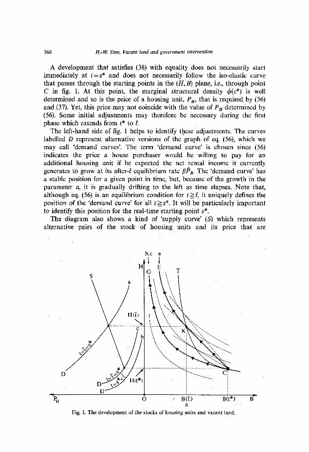
A development that satisfies (38) with equality does not necessarily start immediately at t=s* and does not necessarily follow the iso-elastic curve that passes through the starting points in the (H,B) plane, i.e., through point C in fig. 1. At this point, the marginal structural density (P(E*) is well determined and so is the price of a housing unit, P,, that is required by (36) and (37). Yet, this price may not coincide with the value of P, determined by (56). Some initial adjustments may therefore be necessary during the first phase which extends from t* to E

The left-hand side of fig. 1 helps to identify these adjustments. The curves labelled D represent alternative versions of the graph of eq. (56), which we may call ‘demand curves’. The term ‘demand curve’ is chosen since (56) indicates the price a house purchaser would be willing to pay for an additional housing unit if he expected the net rental income it currently generates to grow at its after-f equilibrium rate BP,. The ‘demand curve’ has a stable position for a given point in time, but, because of the growth in the parameter a, it is gradually drifting to the left as time elapses. Note that, although eq. (56) is an equilibrium condition for t 2 f, it uniquely defines the position of the ‘demand curve’ for ‘all t 2 s *. It will be particularly important to identify this position for the real-time starting point s*.

The diagram also shows a kind of ‘supply curve’ (S’) which represents alternative pairs of the stock of housing units and its price that are

b,c a

H

a

* I ’ B(T) Bit*) B

a Fig. 1. The development of the stocks of housing units and vacant land.

H.-K Sinn, Vacant land and government intervention 369

admissible at time % when a number of further conditions are taken into account. The name ‘supply curve’ is quite arbitrary. It can only be justified insofar as the curve indicates the stock of housing units that for a given housing price would be provided by the market at a point in time f if the growth rates of the stock of housing units and their prices were fixed at their respective after-i? equilibrium values (55) and (57).

In order to derive the ‘supply curve’, it is necessary to consider the possibility of construction activity in the initial meta-time period t* 5 t < s*. Conditions (36), (37), and (39) indicate that during this period the two stock prices P, and P, and the marginal structural density of housing, @(E*), are constants. If combined with the general requirement that the costate variables be continuous functions of time, this constancy has important implications. First, it implies that, in the case of construction activity before s*, (38) takes on the form &*/?/a =PB( 1+ y) throughout the initial meta-time period including the starting point of real time, s *. Because of (54), this property ensures that f=s* and that the equilibrium point in the (H, B) plane moves along one of the iso-elastic curves once real time has begun. Second, the constancy implies that the equilibrium path in the (H,B) plane is linear during the initial meta- time period and is free from kinks even at the point where it joins an iso- elastic curve and where real time starts. Thus, we can conclude that, when there is construction activity before s *, the equilibrium point first moves from point C upward to the left along a negatively sloped straight line, and then continues its movement along the iso-elastic curve to which this line is tangent.

Curve CT in fig. 1 is the locus of admissible tangency points in the (H;B) plane. Quite obviously, a movement up this curve increases both the marginal structural density 4(.s*) chosen before s* and the housing stock H resulting from the initial building activity. Together with (36) and (37), this implies an increasing functional relationship between the housing stock and its price. The graph that depicts this relationship is the ‘supply curve’.

An algebraic expression can be derived for the ‘supply curve’ if we take into account that the constancy of 4(s*) for t Ss* implies

H(K) = 4 c&*m Cm*) - WI + m*)Y (61)

and that, because of (59), the points of tangency have the property

Inserting (61) into (62), applying the inverse function &‘( .) and the lirst- derivative function @( * ) to both sides, and utilizing (37) yields the result

H(i-)(1+6)-H(t*)

B(t*) for H(iT)2H(t*), (63)


where dP,( Q/dH(Q > 0 since 4” < 0, 4’ > 0, and 6 > 0. Note that, while the verbal explanations of the supply curve concentrated on the case H( i?) > H(t*), its mathematical derivation includes the limiting case H(Q = H(t*) in which there is no construction activity during the initial meta- time period and in which even f>s* is possible. Only the case H( 0 c H(t*) has to be excluded in order to take the irreversibility assumption into account. It is also worth noting that, given t *, the functional relationship between P&J and H(Q represented by (63) does not depend on t. Unlike the demand curve, the supply curve will not change its position when time elapses without construction activity taking place.

The first point in real time that the ‘supply’ and ‘demand curves’ have in common marks the border between the two phases. It indicates when and where a movement along an iso-elastic curve in the (H,B) plane will start. If an intersection point above H(t*) exists when real time starts (t =s*), then %=s*, and there is construction activity in the initial meta-time period. This possibility is illustrated by case (a) in fig. 1. In real time, there is an initial jump from C to K and then a gradual movement along the curve KE.

If the two curves have no point in common at time s*, as in case (b) of fig. 1, an immediate start of construction activity at t si;s* is excluded, and (38) cannot hold with equality. Instead, there is a corner solution with ~*/?//a < PB( 1 + y) and F =O. It was shown above, however, that this type of solution cannot persist. Fig. 1 illustrates this. Since the ‘demand curve’ is gradually drifting to the left and the ‘supply curve’ is maintaining its position, the two curves will touch in finite time at the lower end of the supply curve, and by construction this is the point f where (38) holds with equality and where the second phase starts. With regard to the (H,B) plane of fig. 1, this means that the equilibrium point rests for a while at C and will then gradually move along the curve CG as time proceeds.

An intermediate possibility is the case where the supply and demand curves are touching at the lower end of the supply curve when real time starts. In fig. 1 this case is labelled (c). Here, (38) holds with equality at once and hence f=s*. There is neither construction activity in the initial meta- time period nor a halt to construction in real time. The equilibrium point will move along CG once real time has started. Although it may seem very special a priori, this intermediate case must always prevail if the starting point [H(t*),B(t*)] is the outcome of a previously determined path (involving real-time construction) that was calculated with the same information. This follows from the fact that (38) holds continuously once a movement along the ‘right’ iso-elastic curve has started, and is yet another example of the general sub-game perfectness of competitive perfect-foresight equilibria.

The results achieved in this section are summarized in

Proposition 3. In the case of a sufficiently strong growth in the rental demand


for housing [a >= qP[r( l-z) + p]/( 1 - O)], the equilibrium path is characterized - after a potential adjustment phase - by a gradual rise in the stock of housing units, the marginal structural density, the price and rental rate of a housing unit, and the land price, where the growth rate of the latter exceeds the growth rate of the two housing prices. The stock of vacant land is gradually diminishing, but exhaustion occurs only in the limit as time goes to in.nity. The adjustment phase becomes relevant if the equilibrium is disturbed by an unanticipated change in one of the exogenous parameters of the model. The disturbance will result in either a temporary halt to construction or an immediate construction boom.

The gradual exhaustion of vacant land suggests a strong analogy to the theory of natural resources. Note, however, that, because of the specific relationship between the rental market and the land market, this analogy is, in fact, far from being perfect. In the theory of natural resources the resource price is a function of the current extraction volume. Yet the land price in this model is not a function of the current flow of land consumption but rather, via the price of housing units and the rental rate, a function of both the past and the future time paths of this flow. Moreover, the gradual stock depletion is a general phenomenon in market equilibrium models with natural resources and occurs independently of the growth rate in demand. In this model, a gradual stock depletion can only result if the growth rate in rental demand is large enough. If the growth rate is low or even negative, then, according to Proposition 2, there is no vacant land. This aspect also has no counterpart in the theory of natural resources.

6. Market reactions

After going through the details of the solution procedure we can now proceed to study the model’s reactions to exogenous and unforeseen parameter changes. Given the general properties of the solution, it is sufficient, in principle, to consult eqs. (56), (59), and (63), where P, is determined through (41) and 6 through (60). It is, however, also useful to consider the definition of P,, as given in (44), and the two growth equations, (57) and (58). Moreover, we shall repeatedly make use of the facts that the rental rate is directly explained through the stock of housing units [see (35)] and that, in the case of an interior solution, the price of a housing unit, P,, the land price P,, and the marginal structural density c#J(E*) are all positively related to one another [see (36)-(38)].

The analysis is restricted to increases in the respective parameters. Because of the irreversibility assumption, decreases in parameters will generally not yield perfectly symmetric results. The analysis for this case is left to the reader.


6.1. A change in the level of rental demand

Suppose there is an unanticipated increase in the level of rental demand for all t 2s” brought about by a jump in the shift parameter a, given its growth rate. This jump will not affect the position of the ‘supply curve’, but, according to (56), the ‘demand curve’ for the stock of housing units clearly shifts to the left at time s*. The positions the ‘demand curve’ obtains before and after the disturbance are depicted through the curves D and D’ in fig. 2. The intersection point between D’ and the ‘supply curve’, S, determines point K on the line CT, where C is the point at which the disturbance occurred. Hence, there is an immediate jump from C to K and then a gradual movement along the curve KE.

P,(f) 0 W

B

Fig. 2. An increase in the level of rental demand and/or an increase in the rent subsidy.

Along with the rise in the price of housing units, P,, the other prices of the model and the marginal structural density will rise immediately with the increase in rental demand. Thereafter, neither the growth rates of these variables nor those of the stocks of housing units and of vacant land will differ from those that prevailed before and would have continued to prevail without the disturbance.

These straightforward results are summarized in

Proposition 4. An unexpected proportionate increase in rental demand for all future points in time will result in upward shifts of the time paths of the rental rate, the price of housing units, the land price, the marginal structural density, and the stock of housing units, but it will shift the path of the stock of vacant land downward: At each future point in time there will be less vacant land than there otherwise would have been.


6.2. A change in the growth of rental demand

By contrast, assume now that there is an unanticipated increase in the growth rate a of rental demand that is not accompanied by a jump in its level. Unlike the change in the level of rental demand, this disturbance cannot change the position of the (stock) ‘demand curve’ for housing units at the time of the disturbance (s*), but it will affect the ‘supply curve’ and the slope of the iso-elastic curves in the (H,B) plane. Since (60) implies that d6/&2>0, the iso-elastic curves are getting steeper at each point of this plane and the supply durve shifts to the left, from S to S’ in fig. 3. After this reaction, the ‘supply’ and ‘demand curves’ have no point in common, and so there is a halt to construction.

With the passage of time, given the new position of the ‘supply curve’, the ‘demand curve’ drifts to the left, and when it touches the supply curve at point in time f, construction will begin again. Point C in fig. 3 represents the situation where the disturbance occurred. The solution point will rest here for a while and then continue to move upward, albeit with a change from the flatter to the steeper of the two iso-elastic curves depicted in the figure.

H t

S‘ s

‘5 D

PH 0 B

Fig. 3. An increase in the growth rate of rental demand and/or an increase in the income tax rate.

According to (57) and (58), the growth rate of the stock of housing units will increase for the time after t; but despite this the stock of vacant land will shrink at a lower rate. In order for these two aspects to be compatible, the recommencement of construction will have to occur at a higher marginal structural density 4. That this is indeed the case follows from the fact that the temporary halt to construction increases fi to the level fimaX defined in (43) and that hence D is greater for all t >s* than it otherwise would have been. Given the discount rate $1 -r), the higher values of L’ imply that the

R.S.U.E.- C


price of a housing unit, P,, goes up for all tzs* and so landowners choose a higher marginal structural density at f than they otherwise would have done.

A higher marginal structural density and a higher price P, both imply a higher value of P, at time f Since the rate of increase in this price is fixed at the level of the opportunity cost of speculation, the increase in P&) implies an increase in P,(s*), and so the landowners, like the landlords, will enjoy immediate windfall profits.

These findings can be summarized as follows. <

Proposition 5. An increase in the growth rate of rental demand results in a temporary halt to construction. However, when construction begins again, the stock of housing units will grow at an even higher rate than before the stoppage. All price paths, as well as the path of the marginal structural density, shaft upward after the disturbance, and there are immediate windfall profits from both kinds of real estate property. At each point in time after the disturbance the stock of vacant land will be higher than it otherwise would have been, since, in addition to the temporary halt to construction, it is permanently shrinking at a lower rate.

Any mechanical view of real estate markets would suggest that a more rapid growth in rental demand results in an immediate increase in construction activity and in a more rapid decline in the stock of vacant land. Proposition 5 is in striking contrast to this. The reason why it predicts more rather than less vacant land is that a greater growth rate of rental demand signals that needs will be higher in the far distant than in the near future. Both a ‘wise planner’ and well-informed private market agents will therefore experience an increased incentive to preserve vacant land in order to satisfy these needs.

6.3. A rent subsidy

As shown by (56), the introduction or increase of a rent subsidy, 0, will have effects very similar to those of an increase in the level of rental demand, although there is one important difference. While the increase in rental demand results in upward shifts of both the time paths of the net (17) and the gross [( 1 + a)n] rental rates, the increase in (r will clearly shift the time path of the net rental rate downward if, as indicated by (64), the stock of housing units is in elastic ‘supply’.

This condition is completely analogous to the well-known static condition of tax shifting. Note, however, that it implicitly requires vacant land. If there is no vacant land, there cannot be an elastic reaction of the stock of housing units, and the net rental rate II is independent of the subsidy rate at all points in time.

H.-W. Sinn, Vacant land and government intervention 315

Proposition 6. Except for its influence on the time path of the net rental rate, a rent subsidy is equivalent to an equiproportionate increase in the level of rental demand. The subsidy will result in a downward shift ‘of the time path of the net rental rate if vacant land allows for an elastic reaction of the stock of housing units. Without vacant land, it will exclusively benefit the owners of real estate property.

6.4. A general income tax

The introduction or increase of a general income tax, z, on interest and rental income affects the model results primarily through a decrease in the equilibrium rate of growth of the land price, (41). If we assume that there is no tax on the value of vacant land, the quotient PJ(l -T) in (56) remains unchanged, and thus the ‘demand curve’ maintains its position. However, since d6/dPB<0, the supply curve (63) shifts to the left and the iso-elastic curves are getting steeper at each point of the (H, B) plane.

With regard to the time paths of the stock of vacant land, B, and the stock of housing units, H, this results in the same reactions as the increase in the growth rate of rental demand studied above, i.e., construction stops until point in time f after which H rises faster and B shrinks more slowly than without the disturbance. The price reactions and the reaction of the marginal structural density must differ, however, since the decrease in P, requires a decrease in the respective post-f growth rates.

Because of this decrease, an evaluation of the distributional effects of the tax is somewhat ambiguous. During the halt to construction, the rental rate n is rising faster than it would have done without tax increase, but, since fi is being reduced, it is unclear whether tenants will be better off. They will lose in the short run but gain in the long run. Similarly, wealth owners lose insofar as they experience a permanent decline in the effective net rate of return on their assets, but they also enjoy immediate windfall profits on their real estate property.

The existence of windfall profits can be demonstrated as follows. If construction did not stop and the stock of housing units immediately started to grow at its long-run equilibrium rate P,=fi=@,, then eq. (56) would be applicable and it would follow that P,(s*) is constant. However, since fi = fimax during the halt to construction, P,(s*) must rise. As (37) implies that E* is a rising function of Pn, and as (38) indicates that &*/I/a< P,(l + y) if F=O, this means a fortiori that the initial land price, P,(s*), will rise.’

‘In a sense, this result confirms the Johansson-Samuelson theorem on taxation, according to which the value of a given investment project is not affected by the income tax if true economic depreciation deductions are allowed for tax purposes. Since a deduction of economic depreciation is equivalent to a taxation of capital gains, and since the capital gains tax rate is being held constant in the above discussion, the theorem predicts windfall profits for the real estate


Note, finally, that the halt to construction in connection with (56) also implies that P, obtains a higher level at time Z than it would have done without the disturbance. Among other things, this results in a comparatively higher level of the land price and a higher level of the marginal structural density when construction starts again. The main aspects of these results are summarized in

Proposition 7. Given the market rate of interest and given the development of rental demand, the ‘introduction or increase of a tax on interest and rental income implies a temporary halt to construction, immediate jumps in the prices of land and housing units, and a more rapidly growing rental rate. After construction has started again, all prices grow more slowly than before, and the stock of housing units grows at a higher rate. The stock of vacant land will shrink less rapidly and so will be higher at each point in time after the tax increase than it otherwise would have been.

This proposition suggests that income tax systems of the kind that exist in most western countries increase the attractiveness of land speculation and result in excessive holding of vacant land. Thus, if the inefficiencies attri- butable to the holding of vacant land exist at all, they may be the result of a tax distortion rather than a sign of market failure.

6.5. A tax on land consumption

It is one of the basic presumptions of the public finance literature that taxes on land sales and purchases will, like other taxes on transactions, create serious distortions and will therefore not be part of an efficient tax system. This view is certainly accurate for a large class of land transactions. Ilowever, it may be highly misleading insofar as the transactions tax has the character of a tax on the consumption of vacant land for construction purposes.

Indeed, an inspection of conditions (51), (56), and (63) shows that the introduction or increase of the tax rate y, which applies to the land purchases on the part of landlords, would not have any real effects in the present model. Thus, tax revenue can be obtained without incurring any welfare reducing distortions.

It is an implication of this neutrality result that the incidence of the tax falls exlusively on the landowners. Given the time path of the marginal value product of land, ~*/?/a, the time path of the gross land price P,(l + y) is well determined, and hence the entire path of the net price of land, P,, has to

owners provided they do not react to the tax. In the present model, this prediction holds even though considerable reactions on the part of market agents occur. See Johansson (1961) and Samuelson (1964).


move downward sufficiently to allow for a 100% shifting of the tax. These implications yield

Proposition 8. In its function as a tax on land consumption for construction purposes, the land sales or purchase tax is allocatively neutral. Landowners bear the entire burden of this tax.

The economic reason behind this neutrality result is that the tax is virtually a cash-flow tax on vacant land.9 Given the general fact that, in a market equilibrium, the allocative effects of a tax will not depend on its formal incidence, the tax on land consumption in effect makes government a silent partner in the ownership of vacant land. This partnership is clearly a disadvantage for landowners, but there is no way for them to alter the present value of the tax burden.

Occasionally it is argued that the tax will provide an incentive for postponing the sales date since, in the presence of discounting, this would reduce the present value of the tax. This argument, however, clearly overlooks the fact that a rise in the price of land will increase the tax payment when the transaction is postponed. Since, in a market equilibrium, the landowner is indifferent with regard to the selling date, and since the tax payment is proportional to the sales price, the increase in the tax payment will be just enough to compensate for the discounting.

6.6. A tax on the value of vacant land

A classical means used by policymakers to force the mobilization of vacant land is the tax on the value of the stock of vacant land (p). This tax increases the opportunity cost of land speculation and results in a rise in the equilibrium rate of increase in the land price, pB. This rise may violate the growth condition (51) and may induce an immediate construction boom that consumes all the vacant land available.

If the growth condition is not violated, there will be a less dramatic reaction. Since (60) implies that dd/dpB<O, the iso-elastic curves are becom- ing flatter at each point of the (H,B) plane and, according to (63), the ‘supply curve’ for housing units shifts to the right, from S to S’ in fig. 4. At the same time, (56) requires a shift of the ‘demand curve’ to the left, from D to D’. Because of the change in the slopes of the iso-elastic curves, the tangency curve CT pivots to the left into the new position CT’. The new intersection point between the ‘supply’ and ‘demand curves’ is point K on this curve and

9Note that in order to preserve the cash-flow character of the tax in a more realistic environment it would be necessary to allow for a deduction of current expenses and to include the current revenue from the vacant land in the tax base. A pure sales tax would no longer be completely distortion-free in such an environment.


A

H E T’ T

s s’

(2&k*

K

t ‘_

D‘ . . . . .._....................... C

D

PH 0 0 B

Fig. 4. An increase in the tax on vacant land and/or the capital gains tax rate.

characterizes the end of the (fictive) initial meta-time period. The optimal path after the tax increase thus implies an immediate jump from C to K and then a gradual movement up the curve KE. During this gradual movement, fi, p,, and 6 are higher than before and, according to (57) and (58), fi and B are lower, where, since B<O, the latter indicates an increase in the rate at which the stock of vacant land is diminishing.

The incidence of the tax is ambiguous. The construction boom will result in an immediate decrease in the rental rate II, but since the growth rate fi is rising along with P,, there is a finite point in time beyond which the rental rate will be higher than it otherwise would have been. Being derived from the path of 17, the initial values of stock prices P, and P, will therefore be ambiguous. In the long run, of course, they will be lower than they would have been without the tax increase.

Proposition 9. The introduction of a tax on vacant land results in an immediate construction boom. If the tax is sufficiently high, this boom leads to an immediate exhaustion of all vacant land, but with a moderate tax, some of the land will be absorbed immediately, and the remaining stock will shrink at a higher rate. In the latter case the growth rate of the stock of housing units is reduced, but the growth rates of all prices and the marginal structural density are increased. There are no unambiguous advantages for tenants since, despite the short-run construction boom, in the long run the stock of housing units will be lower and the rental rate higher than they would have been in the absence of the tax.

6.7. .A capital gains tax on vacant land

Among the taxes considered in this paper, the capital gains tax (0) has been given by far the most attention in the policy oriented literature on the


vacant land problem. lo Like the tax on the value of vacant land, this tax becomes operative only through increasing the opportunity cost of speculation and requires a higher equilibrium rate of increase in the land price, (41). It is quite obvious that this results in the same model reactions as those described in fig. 4 and Proposition 9. Thus we can state:

Proposition 10. A tax on accrued capital gains from land appreciation is equivalent to a tax on the value of vacant land.

This proposition ensures that the capital gains tax will indeed, as many authors have conjectured, reduce the stock of vacant land. However, it shows also that the capital gains tax, like the tax on vacant land, requires the initial boom in construction to be paid for through a comparative long-run decline in the housing stock and a rise in the rental rate. This aspect clearly dampens the overly favorable expectations held by some of the authors on the virtues on this tax.

Note that the tax modeled in this paper is a tax on accrued capital gains and not a tax on realized capital gains alone. Many economists have objected to the latter, arguing that it provides strong incentives for a withholding of land.ll This view seems at least doubtful. On the one hand, if the tax induces landowners to keep their land and build on it themselves, the tax will not affect the decision when to build. On the other hand, given that landowners want to sell some day despite the tax, it would be better for them to do it sooner than later. This follows from the fact that the tax on realized capital gains is equal to a tax on the value of land consumption where the historical purchasing price is tax-deductible. As the tax on land consumption is allocatively neutral (Proposition 8), only the tax deductibility of the given historical purchasing price will affect the landowner’s decision. Thus, the allocative results of the tax on realized capital gains are equal to those of a fixed sales premium, and this will clearly provide an incentive to sell the land earlier. With regard to the mobilization of vacant land there will therefore be no substantial difference between the two kinds of capital gains taxes.

6.8. The income tax and the capital gains tax

As shown above, a simple income tax (r) that is imposed on interest and rental income is non-neutral in that it induces a substitution of future for current housing consumption. An attempt might be made to compensate for

‘OAn overview of the literature is given, in German, by Friauf, Risse and Winters (1977). “A different opinion was expressed by Schneider (1976), though. Moreover, it was shown by

Markusen and Scheffman (1978) that the tax on realized capital gains will reduce the incentive to withhold the land in a two-period model.


this effect through a more favorable tax treatment of rental income, and indeed this is the approach chosen in the United States and some other countries. The problem with such a measure is, however, that it increases the demand for housing at all points in time and will not induce an intertemporal substitution effect that can provide the desired compensation. This is evident from the analysis of subsection 6.3 if we note that, in the present model, a tax exemption of rental income would be equivalent to a rent subsidy 0. Such a subsidy increases the equilibrium stock of housing units, but it does so for all points in time. I

A more suitable measure for compensating the effects of the income tax might be the capital gains tax for vacant land since, as shown above, this tax induces a substitution of present for future housing consumption. Suppose, therefore, that interest income, rental income, and capital gains from land appreciation are subject to the same tax, z=w >O, where, in order to satisfy the existence condition (52), it is assumed that the tax rate falls short of the share of construction expenses in the total cost .of a housing unit (o < IX) and that there is no tax on the value of vacant land (p =O). It follows from (41) that this combination of taxes does not affect the equilibrium rate of growth in the land price, b,, and hence neither the iso-elastic curves in the (H,B) plane nor the ‘supply curve’ are subject to changes. However, according to (56), the ‘demand curve’ will clearly shift to the left. Except for the gross rental rate L!(l + o) whose time path will be shifted downward along with that of the net rental rate n, this will result in the same reactions as those analyzed in subsection 6.3. Hence we can state

Proposition 11. A uniform tax on interest income, rental income, and accrued capital gains from the appreciation of vacant land brings about the same results as a rent subsidy in terms of real allocation effects and reactions of the net rental rate, the price of a housing unit, and the land price.

It follows from this proposition and the analysis of subsection 6.3 that the capital gains tax on vacant land is indeed able to compensate for the substitution effect which results from the income tax. But, in addition, it produces an equiproportionate increase in the housing stock for all points in time. Because of this increase, the inclusion of accrued capital gains on vacant land in the income tax base is also non-neutral.

In order to induce neutrality it would be necessary either to impose an additional rent tax (0~0) on the landlords or to increase the income tax base even further by also including the appreciation in the value of housing units. The latter would ensure that income taxation is strictly in line with the Schanz-Haig-Simons concept, and it is well known from the Johansson- Samuelson theoremI that this concept ensures an intersectoral neutrality of taxation.13


7. Concluding remarks

The baker distributes bread among the starving in a manner not unlike the speculator distributing land among the builders. Under certain ideal conditions, both satisfy the task of allocating a scarce resource efficiently among competing uses. The fact that the consumption of land is postponed and the consumption of bread is not, does not necessarily indicate market failure, it may instead be a direct efficiency requirement if construction is irreversible and rental demand for housing is growing fast.

It is true that speculative activity may withhold too much vacant land compared to a Pareto optimum. However, the present analysis suggests that if this happens it is more likely to be a distortion brought about by the income tax than by market failure. Since the income tax discriminates less against savings in the form of real estate property than against savings in the form of other capital goods, it may well induce an excessive speculative commitment. As shown in the paper, this can be compensated for by introducing additional taxes on real estate property. However, it is also possible of course to abolish the discrimination against savings in general by introducing one of the cash-flow type income tax systems that have been proposed in recent years by a number of authors and tax committees. From an overall perspective this possibility, which gets at the cause of the problem, seems more promising than policies which simply alleviate the symptoms.

Appendix 1: Derivation of the stock-growth equations

Differentiating (56) logarithmically and using (11) yields

E?=d-y&. (A4

Eq. (57) follows from this if pH is replaced according to (55):

E?=&r@,>O. (A.2)

That E? is strictly positive is implied by the assumption that the growth in rental demand is sufficiently fast to satisfy (51).

Since (A.2) and (41) indicate that fi=const., it follows that

A&. (A.3)

“See Johansson (1961) and Samuelson (1964). r3Note that an intersectoral neutrality of taxation is not necessarily desirable for an efficient

tax system since there may be a conflict between intersectoral and intertemporal requirements. For detailed analyses of this conflict see Hamilton and Whalley (1985) and Long and Sinn (1984).


On the other hand, (4) and (5) imply

IL$+Lx,_+R (A.4)

Combining (A.2), (A.3), and (A.4) yields

P = ci - B,(qp + a) = const.

To establish the sign of E, note that it follows from (41) that

(A.5)

B&(1-z), (A.6)

and that assumption (53) implies

fi<x-& (A.7)

where X is defined in (52). Using this definition and noting that (A.6) and (A.7) result in

P<X-ar(l-z), (A.@

we obtain

P< -r(l-+0-j+. (A.9)

Since r, z, co, p, y 2 0 this implies that

P<O. (A. 10)

In order to derive the growth equation for B, note that (8) gives F = -& and that the slope of the path of land exhaustion in an (F,B) plane is hence given by

dFP P_p - dB=z=-F= . (A.11)

Since fi = const., this equation ensures that the flow of land consumption is a linear function of the stock of vacant land,

F=a,+a,B, (A. 12)

where a2 = -_=const. >O. If a, >O, the stock of vacant land is exhausted in finite time, a case excluded by Proposition 2. If a, ~0, some of the vacant


land will never be built upon. This violates the transversality condition in the planning problem of the landowner [(33) or (42)] which requires that

lim B(t) = 0, (A.13) t+cC

since, according to (41), p,Zr(l -z). Hence, a, =0 and

F=a,B. (A.14)

An immediate implication of this is B =@B = -F/B = - a2 = P or, using (A.5) and (A.lO),

B=ii-P~(~~+a)<o. (A.15)

Appendix 2: Existence conditions

It will now be shown that, given the assumptions made in the text and given the results of Appendix 1, the transversality conditions (2) are satisfied.

Using (A.2) and (55) it follows from (42) that the transversality condition in the problem of the landlord is satisfied if and only if

d-~j3B,-x*<o, (A.16)

where

x*=r(l-r)-@B. (A.17)

Since the case considered in subsection 5.2 is characterized by B >r/?P, from (51), it is necessary, though not sufficient, for (A.16) to hold that

x*>o. (A.18)

Inserting pB from (41) into (A.17) and using CI = 1 -j? from (7), we find that

x*=x, (A.19)

where, according to assumption (52),

Xzr(l--)(a-co)-jlpp>O. (A.20)

Thus, the necessary condition (A.18) is satisfied. Note that this also implies that the denominator of (56) is strictly positive.


In addition to (A.20) it was assumed with (53) that

a<x+r/pB,. (A.21)

Because of (A.19), this assumption is equivalent to (A.16). It is therefore necessary and sufficient for the transversality condition of the landlord to be satisfied.

A further implication of (42) is T,,

P,+B-i-(1-z)<O. (A.22)

This condition is the transversality condition of the landowner. Inserting (A.15) into (A.22) and using a= 1-b from (7), we find that (A.22) is equivalent to

b-r@,-X” <o, (A.23)

which is the same as (A.16). Thus, the transversality condition of the landowner is satisfied.

References

Amott, R.J., 1980, A simple urban growth model with durable housing, Regional Science and Urban Economics 10, 53-76.

Amott, R.J. and F.D. Lewis, 1979, The transition of land to urban use, Journal of Political Economy 87, 161-169.

Brueckner, J.K. and B.. von Rabenau, 1981, Dynamics of land-use for a closed city, Regional Science and Urban Economics 11, 1-17.

Dietrich, H., K. Hoffmann and H. Junius, 1981, Fallstudien zum Baulandpotential fur stadtischen Lticken-Wohnungsbau, Schriftenreihe ‘Stldtebauiiche Forschung’ des Bundes- ministers fur Raumordnung, Bauwesen und Stldtebau (Bad Godesberg).

Friauf, K.H., W.K. Risse and K.-P. Winters, 1977, Der Beitrag steuerlicher MaOnahmen zur Losung der Bodenfrage, Schriftenreihe ‘Stldtebauliche Forschung’ des Bundesministers fur Raumordnung, Bauwesen und StHdtebau (Bad Godesberg).

Fujita, M., 1976, Spatial patterns of urban growth: Optimum and market, Journal of Urban Economics 3, 203-241.

Hamilton, B. and J. Whalley, 1985, Tax treatment of housing in a dynamic sequenced general equilibrium model, Journal of Public Economics 27, 157-175.

Johansson, S.-E., 1961, Skatt-investering-vardering (Stockholm). Kamien, M.I. and N.L. Schwartz, 1981, Dynamic optimization (North-Holland, Amsterdam). Long, N.V. and H.-W. Sinn, 1984, Taxation and economic depreciation: A general equilibrium

model with capital and an exhaustible resource, in: M.C. Kemp and N.V. Long, eds., Essays in the economics of exhaustible resources (North-Holland, Amsterdam).

Markusen, J. and D. Scheffman, 1978, The timing of residential land development: A general equilibrium approach, Journal of Urban Economics 5, 41 l-424.

Mills, D.E., 1981, Growth, speculation and sprawl in a monocentric city, Journal of Urban Economics 10,201-226.


Ohls, J.C. and D. Pines, 1975, Discontinuous urban development and economic efficiency, Land Economics 51, 224-234.

Oppenheimer, F., 1910, Theorie der reinen und politischen i)konomie (Reimer, Berlin). Samuelson, P.A., 1964, Tax deductibility of economic depreciation to insure invariant valu-

ations, Journal of Political Economy 72, 604-606. Schneider, D., 1976, Besteuerung von VerauBerungsgewinnen und Verkaufsbereitschaft: der

fragwtirdige ‘lock-in-Effekt’, Steuer und Wirtschaft 53, 197-210. Shoup, D.C., 1970, The optimal timing of urban land development, in: M.D. Thomas, ed., The

Regional Science Association Papers 25, 3344. Sinn, H.-W., 1984, Das Bauliickenproblem. Eine allokationstheoretische Untersuchung zur

Funktionsweise des Baumarktes und zu den Miiglichkeiten seiner Regulierung, in: M. Neumann, ed., Ansprtiche, Eigentums- und Verftigungsrechte (Duncker und Humblot, Berlin).

Weber, A., 1908, Boden und Wohnung (Duncker und Humblot, Leipzig). Wheaton, W.C., 1982, Urban residential growth under perfect foresight, Journal of Urban

Economics 12, 1-21.

Documents

Vacant Land and the Role of Government Intervention · Vacant Land and the Role of Government Intervention by Hans-Werner Sinn ... market equilibrium model that records fully the