Center/or Turbulence Research

Proceedings o/ the Summer Program 1996

./.v2L/35

A new approach to turbulence modeling

By B. Perot 1 AND P. Moln 2

A new approach to Reynolds averaged turbulence modeling is proposed which has

a computational cost comparable to two equation models but a predictive capability

approaching that of Reynolds stress transport models. This approach isolates the

crucial information contained within the Reynolds stress tensor, and solves trans-

port equations only for a set of "reduced" variables. In this work, direct numerical

simulation (DNS) data is used to analyze the nature of these newly proposed tur-

bulence quantities and the source terms which appear in their respective transport

equations. The physical relevance of these quantities is discussed and some initial

modeling results for turbulent channel flow are presented.

1. Introduction

I.I Background

Two equation turbulence models, such as the k/e model and its variants, are

widely used for industrial computations of complex flows. The inadequacies of these

models are well known, but they continue to retain favor because they are robust

and inexpensive to implement. The primary weakness of standard two equation

models is the Boussinesq eddy viscosity hypothesis: this constitutive relationship is

often questionable in complex flows. Algebraic Reynolds stress models (or non-linear

eddy viscosity models) assume a more complex (nonlinear) constitutive relation for

the Reynolds stresses. These models are derived from the equilibrium form of the

full Reynolds stress transport equations. While they can significantly improve the

model performance under some conditions, they also tend to be less robust and

usually require more iterations to converge (Speziale, 1994). The work of Lund

Novikov (1992) on LES subgrid closure suggests that even in their most general

form, non-linear eddy viscosity models are fundamentally incapable of completely

representing the Reynolds stresses. Industrial interest in using full second moment

closures (the Reynolds stress transport equations) is hampered by the fact that

these equations are much more expensive to compute, converge slowly, and are

suscet)tible to numerical instability.

In this work, a turbulence model is explored which does not require an assumed

constitutive relation for the Reynolds stresses and may be considerably cheaper to

compute than standard second moment closures. This approach is made possible

by abandoning the Reynolds stresses as the primary turbulence quantity of interest.

1 Aquasions Inc., Canaan NH

2 Center for Turbulence Research

https://ntrs.nasa.gov/search.jsp?R=19970014654 2018-08-09T01:02:08+00:00Z

36 B. Perot _ P. Moin

The averaged Navier-Stokes equations only require the divergence of the Reynolds

stress tensor, hence the Reynolds stress tensor carries twice as much information as

required by the mean flow. Moving to a minimal set of turbulence variables reduces

the overall work by roughly half, but introduces a set of new turbulence variables,

which at this time are poorly understood. This project attempts to use DNS data

to better understand these new turbulence variables and their exact and modeled

transport equations.

1.2 Formulation

The averaged Navier-Stokes equations take the following form for incompressible,

constant-property, isothermal flow:

V. u = 0 (1.)

0u

0--t- + u. Vu = -Vp+ uV. S- V- R (lb)

where u is the mean velocity, p is the mean pressure, u is the kinematic viscosity,

S = Vu + (Vu) T is twice the rate-of-strain tensor, and R is the Reynolds stress

tensor. The evolution of the Reynolds stress tensor is given by:

OR

Ot--+u. VR=uV2R+P-•+I-I-V-T-[Vq+(Vq) T] (2)

where P is the production term, • is the (homogenex_us) dissipation rate tensor,

II is the pressure-strain tensor, T is the velocity triple-correlation, and q is the

velocity-pressure correlation. The last four source terms on the right-hand side

must be modeled in order to close the system. The production term P is exactly

represented in terms of the Reynolds stresses and the mean velocity gradients. This

is the standard description of the source terms, but it is by no means unique and

there are numerous other arrangements.

Note that turbulence effects in the mean momentum equation can be represented

by a body force f = V' • R. One could construct transport equations for this body

force (which has been suggested by Wu et al., 1996), but mean momentum would no

longer be simply conserved. To guarantee momentum conservation, the body force

is decomposed using Helmholtz decomposition, into its solenodal and dilatational

parts, f = V¢ + V × ¢. A constraint (or gauge) must be imposed on _b to make the

decomposition unique. In this work we take V • _, = 0. With this choice of gauge,

the relationship between ¢ and ¢ and the Reynolds stress tensor is given by,

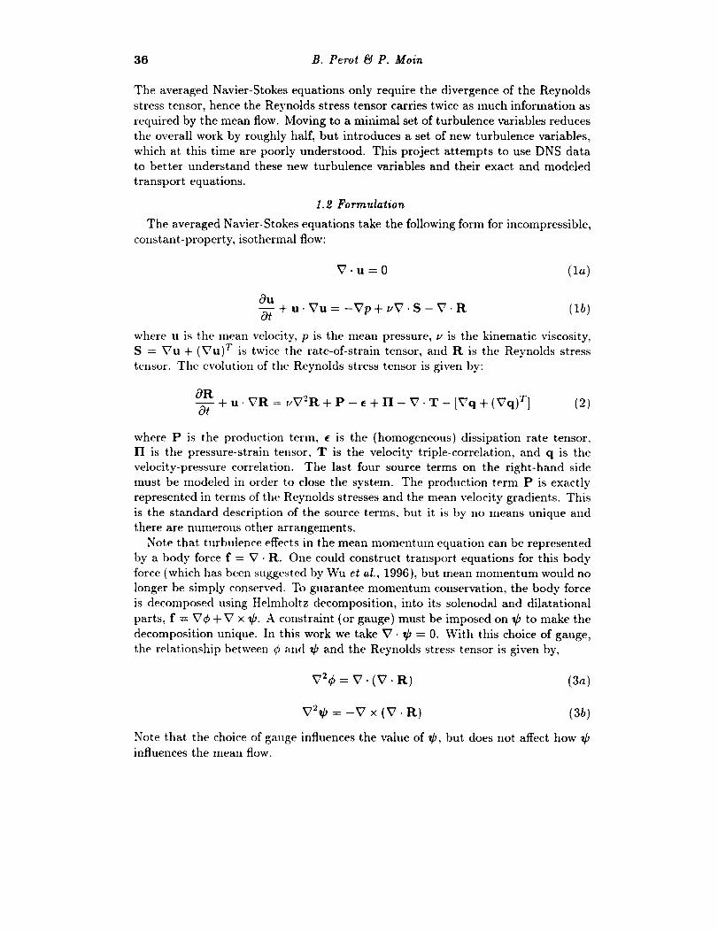
V2¢ = V-(V. R) (3a)

V_¢ = -V × (V-R) (3b)

Note that the choice of gauge influences the value of ¢, but does not affect how _b

influences the mean flow.

A new approach to turbulence modeling 37

Using these relationships, transport equations for ¢ and _ can be derived from

the Reynolds stress transport equations.

0¢_-+u.V¢=vV2¢-2V.q-V-2V .V.[c-II+V.T-P]+V-2Sv (4a)

0¢+u.V¢=vV2¢+Vxq+V-2VxV.[¢-II+V.T-P]+V2S¢ (4b)

These equations contain extra production-like source terms S¢ and S_ which contain

mean velocity gradients. Note that the production term is not an explicit function

of ¢ and ¢ (except under limited circumstances) and, in general, must be modeled.

The inverse Laplacian V -2 that appears in these equations can be thought of as an

integral operator.

2. Theoretical analysis

2.1 Turbulent pressure

Taking the divergence of Eq. (lb) (the mean momentum equation) gives the

classic Poisson equation for pressure,

v2p = -v. (u. v.) - v. (v. R) (5)

Since this is a linear equation, the pressure can be split conceptually into two terms:

one can think of the mean pressure as being a sum of a mean flow pressure due to

the first term on the right-hand side,

V2pmean = --V" (u. Vu) (6a)

and a turbulent pressure due to the second term on the right-hand side,

v2P,. s = -v. (v. R) (6b)

Given the definition of ¢ and assuming that ¢ is zero when there is no turbulence,

then it is clear that ¢ = -Pt,,,-b. For this reason, ¢ will be referred to as the

turbulent pressure. This quantity is added to the mean pressure in the averaged

momentum equation, which results in Pro,,,, = p + ¢ being the effective pressure

for the averaged equations. The quantity P, nean tends to vary more smoothly than

p, which aids the numerical solution of these equations.

For turbulent flows with a single inhomogeneous direction, the turbulent pressure

can be directly related to the Reynolds stresses. In this limit Eq. (3a) becomes

¢,22 = R22,22 where x2 is the direction of inhomogeneity. This indicates that ¢ =

R22 for these types of flows. Note that R22 is positive semi-definite, so ¢ is always

greater than or equal to zero in this situation. Positive ¢ is consistent with the

picture of turbulence as a collection of random vortices (with lower pressure cores)

embedded in the mean flow. It is not clear what the conditions for a negative

turbulent pressure would be, if this condition is indeed possible.

38 B. Perot _ P. Moin

2.2 Turbulent vorticity

To understand the role of _b it is instructive to look again at turbulent flows that

have a single inhomogeneous direction. Under this restriction Eq. (3b) becomes

_i,z2 = -ei2kRk2,22 where x2 is the direction of inhomogeneity. If _b goes to zero

when there is no turbulence then g'i = -ei2kRk2, (or _"l : -R32, g'2 = 0 and

_h3 = R12). These are the off diagonal, or shear stress components of the Reynolds

stress tensor.

For two-dimensional mean flows with two inhonlogeneous flow directions, only

the third component of _b is non-zero, and Eq. (3b) becomes

t/'3,11 -_- _'3,22 _-- R12,22 - RI2,11 + (RII - R22),12 (7)

Since _ is responsible for vorticity generation, it is appropriate that it be aligned

with the vorticity in two-dimensional flows. As a first level of approximation, it is

not unreasonable to think of _ as representing the average vorticity of a collection

of random vortices making up the turbulence, and therefore _ will be referred to

as the turbulent vorticity.

For two-dimensional flows with a single inhomogeneous direction g'a = R12.

Note how the components of _b reflect the dimensionality of the problem, while the

mathematical expressions for these components reflects the degree of inhomogeneity.

2.3 Relationship with the eddy viscosity hypothesis

The linear eddy viscosity hypothesis for incompressible flows takes the form,

9

R = -ur(Vu + (Vu) 7") + 2_'I (8)3

where UT is the eddy viscosity, I is the identity matrix, and _' is one half the trace

of the Reynolds stress tensor.

Taking the divergence of Eq. (8) and rearranging terms gives,

9

f = V. R = V(-_lc - 2u. VuT) + V x (urV x u) + 2u. V(Vur). (9)

If the eddy viscosity vanes relatively slowly, as is usually the case, then the very last

term (involving the second derivative of the eddy viscosity) will be small and can be

neglected. Under these circumstances the linear eddy viscosity model is equivalent

to the following model,,)

¢ = _/_- - 2u. Vur (10a)

_b = urV x u. (10b)

So to a first approximation the turbulent vorticity, ¢ should be roughly equal to the

mean vorticity, times a positive eddy viscosity; and the turbulent pressure should

be roughly equal to two thirds of the turbulent kinetic energy. These results are

entirely consistent with the findings of the previous subsections.

A new approach to turbulence modeling 39

PHI

PSI

FIGURE 1. Contours of turbulent pressure (0) and negative t urbuh'nt vorticity

(-_b) for the separating boundary layer of Na & Moin.

3. Computational results

Equations (3a) and (3b), relating the turbulent pressure and turbulent vorticity

to the Reynolds stresses, were used to calculate ¢ and !b from DNS data for two

relatively complex two-dimensional turbulent flows: a separating boundary layer

(Na & Moin, 1996) and flow over a backward facing step (Le & Moin, 1995). The

purpose was to assess the behavior of these turbulence quantities in practical tur-

bulent situations, and to provide a database of these quantities fi)r later c()mt)arison

with turbulence models.

3.1 Separated boundary layer

The values of ¢ and -_3 are shown in Fig. 1. As mentioned previously, for two-

dimensional flows only the third component of _ is nonzero. The flow moves from

left to right, separates just before the midpoint of the computational domain, andthen reattaches before the exit. The contours are the same for both quantities and

range from -0.0004U_ to 0.0lUg, where U_ is the inlet free-stream velocity.

Both the turbulent, pressure and turbulent vorticity magnitudes increase in the

separating shear layer and the reattachment zone. In addition, both quantities

become slightly negative in the region just in front (to the left.) of the separating

shear layer, and show some "elliptic" (long range decay) effects at the top of the

separation bubble. There is some speculation at this time that these effects could

be numerical, but there is also some reason to believe that they are a legitimate

result of the elliptic operators which define these variables. Changes in the far-

field boundary condition (from zero value to zero normal gradient) had no visibly

perceptible effect on the values of d and _!'3.

The visual ot)servation that & and -_'3 are roughly proportional is analogous to

the observation that 0.3k .._ -R12 (originally developed by Townsend, 1956, and

successfully used in the turbulence model of Bradshaw, Ferriss & Atwei1, 1967).

40 B. Perot _ P. Moin

-R12

FIGURE 2. Contours of tile normal Reynolds stress (R22) and negative turbulent

shear stress (-R12) for the separating boundary layer of Na &: Moin.

It is also consistent with the (first order) notion of turbulence as a collection of

embedded vortices, with -¢ representing the average vortex core pressure and ¢

representing the average vortex strength.

In the case of a single inhomogeneous direction, ¢ = R22 and ¢3 = R12. It is

instructive therefore to compare the results shown in Fig. 1 with the R22 and -R12

components of the Reynolds stress tensor, shown in Fig. 2. The magnitudes of

the contours in Fig. 2. are the same as Fig. 1. This comparison clearly shows the

additional effects that result from inhomogeneity in the streamwise direction. The

leading and trailing boundary layers (which have very little streamwise inhomogene-

ity) are almost identical. However, the magnitudes of the turbulent pressure and

turbulent vorticity are enhanced in the separated shear layer due to the streamwise

inhomogeneity.

3.2 Backward facing step

Computations of ¢ and -tL'3 for the backward facing step are shown in Fig. 3. The

flow is from left to right, and there is an initial (unphysical) transient at the inflow

as the inflow boundary condition becomes Navier-Stokes turbulence. The boundary

layer leading up to the backstep has moderate levels of the turbulent pressure and

turbulent vorticity (which closely agree with the values of R22 and -R12 in that

region). As with the separating boundary layer, the turbulent pressure and turbu-

lent vorticity increase significantly in the separated shear layer and reattachment

zone. There is an area of slight positive turbulent pressure and negative turbulent

vorticity in the far field (about one step height) above the backstep corner. This

may or may not be a numerical artifact, and is discussed in the next section.

3.3 Ellipticity

Identifying the exact nature of the ellipticity of these new turbulence quantities is

important to understanding their overall behavior and how they should be modeled.

A new approach to turbulence modeling 41

PHI

PSI

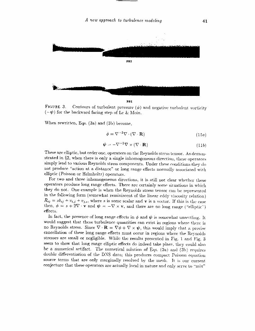
FIGURE 3. Contours of turbulent pressure (¢) and negative turbulent vorticity(-¢) for the backward facing step of Le & Moin.

When rewritten, Eqs. (3a) and (3b) become,

¢ = v-2v. (v. R) (11a)

¢ = -V-2V × (V-R) (llb)

These are elliptic, but order one, operators on the Reynolds stress tensor. As demon-

strated in §2, when there is only a single inhomogeneous direction, these operators

simply lead to various Reynolds stress components. Under these conditions they do

not produce "action at a distance" or long range effects normally associated with

elliptic (Poisson or Helmholtz) operators.

For two and three inhomogeneous directions, it is still not clear whether these

operators produce long range effects. There are certainly some situations in which

they do not. One example is when the Reynolds stress tensor can be represented

in the following form (somewhat reminiscent of the linear eddy viscosity relation)

R,j = sSij + v,,j + vj,i, where s is some scalar and v is a vector. If this is the case

then, ¢ = s + 22 7 • v and ¢ = -27 × v, and there are no long range ("elliptic")effects.

In fact, the presence of long range effects in ¢ and _b is somewhat unsettling. It

would suggest that these turbulence quantities can exist in regions where there is

no Reynolds stress. Since V. R = 27¢ + 27 x ¢, this would imply that a precise

cancellation of these long range effects must occur in regions where the Reynolds

stresses are small or negligible. While the results presented in Fig. 1 and Fig. 3

seem to show that long range elliptic effects do indeed take place, they could also

be a numerical artifact. The numerical solution of Eqs. (3a) and (3b) requires

double differentiation of the DNS data; this produces compact Poisson equation

source terms that are only marginally resolved by the mesh. It is our current

conjecture that these operators are actually local in nature and only serve to "mix"

42 B. Perot _J P. Moin

"g

= 0.0000. w4

0"0050 / , ,

0.0025

!

-0.0025,,, ...: _.: ._"

-0.00500.0 0.5 1.0 1.5 2.0

y/h

FIGURE 4. Budget of the ¢ transport equation at a station roughly half way

through the recirculation bubble of the backward facing step (x/h = 4.0). --'-- dis-

sipation or diffusion; .... velocity pressure-gradient; ........ triple correlation term;

--production (positive) or convection.

various components of the Reynolds stress tensor. It is also conjectured from these

computational results that the turbulent pressure is a positive semi-definite quantity.Note that the ellipticity discussed here is not the same as an ellipticity in the

governing evolution equations for these quantities. An elliptic term in the evolutionequations is both physical and desirable (see Durbin, 1993). Such a term mimics

long range pressure effects known to occur in the exact source terms. The exact

evolution equations for ¢ and _, described below, have just this elliptic property.

3.4 Turbulent pressure evolution

Considerable insight can be obtained about the evolution of the turbulent pres-

sure by considering the case of a single inhomogeneous direction. It has been shownthat under these circumstances ¢ = R22, so the evolution is identical with the

Reynolds stress transport equation for the normal Reynolds stress, R22. For thecase of turbulent channel flow (Mansour et al., 1988), the R22 evolution is domi-

nated by a balance between dissipation and pressure-strain, with somewhat smallercontributions from turbulent transport and viscous diffusion. There is considerable

interest in determining if these same trends continue for ¢ evolution in more com-

plex situations, since the ultimate goal is to construct a modeled evolution equation

for this quantity.

Figure 4 shows the terms in the exact ¢ evolution equation for flow over a back-ward facing step, at a station roughly in the middle of the recirculation bubble.These terms were calculated in the same manner as the turbulent pressure. Both

A new approach to turbulence modeling 43

0.015 i

0.010 ..................................._" ........ ".................÷...........................................................................

0.005.....-::::::J,..........................................i..............................................................

= 0.000

-0.005 -

-0.010-

-0.015 ,0.0 0.5 1.0 1.5 2.0

y/h

FIGUltE 5. Budget of the Oa transport equation at a station roughly half way

through the recirculation bubble of the backward facing step: see Fig. 4 for caption.

the detached shear layer and the backward moving boundary layer are visible in the

statistics. In the shear layer, the expected dominance of dissipation and pressure-

terms (presumably dominated by pressure-strain) is evident. In the recirculating

boundary layer, turbulent transport and pressure-terms (probably dominated by

pressure transport) are dominant. It is interesting to note that the production termdominates in the middle of the recirculation bubble. The fact that some of these

source terms are not exactly zero at roughly two step heights away from the bottom

wall is thought to be a numerical artifact similar to those found when calculating

¢ and ¢. Some of the curves have an erratic nature due to the lack of statisti-

cal samples. This phenomena is also present in the (unsmoothed) Reynolds stress

transport equation budgets presented in Le &: Moin, 1993.

3.5 Turbulent vorticity evolution

As with the turbulent pressure, it is useful to consider the case of a single inhomo-

geneous direction when analyzing the evolution of the turbulent vorticity. Under

these circumstances ¢3 evolves identically to the Reynolds shear stress, R12. In

turbulent channel flow, the R12 evolution is dominated by a balance between pro-

duction and pressure-strain, with somewhat smaller contributions from turbulent

and pressure transport. This trend continues in the ¢3 evolution equation, which

is shown in Fig. 5., for the backward facing step at a cross section roughly halfway

through the recirculization bubble (x/h = 4.0). The small value of the dissipation

is consistent with the fact that isotropic source terms can be shown not contribute

to the evolution of ¢.

44 B. Perot _ P. Moin

4. Modeling

4. i Formulation

An initial proposal for modeled transport equations for the turbulent pressure

and turbulent vorticity are,

0-7 +u.Vo = V.(v+p,r)V¢- C, _- \ v2 / _+ 15v + vT

oo (;_)-_-+u-V¢=V.(V+VT)V_b- ¢'- _-T g' +¢w (12b)

where, C_ = 0.09, y is the normal distance to the wall, the time-scale is given by T =

(t/+ t,T)/¢, and the eddy viscosity is given by "7" = Ig'l/]_]. Dissipation (and some

redistribution) is modeled as an exponential decay process (roughly corresponding to

Rotta's, low Reynolds nmnber dissipation model). Turbulent and pressure transport

are collectively modeled as enhanced diffusive transport. Production and energy

redistribution are proportional to the turbulence pressure times the mean vorticity

for the turbulent vorticity, and are proportional to the square of the turbulent

vorticity magnitude for the turbulent pressure. High Reynolds number constants are

determined so that ¢ = 2k at high Reynolds numbers. The low Reynolds number

constants (which appear with a v) are set to obtain exact asymptotic behavior and

good agreement with the channel flow simulations of the next section.

Note that both ¢ and _ have the same units. An extra turbulent scale is currently

defined by using the mean flow timescale Iwl to define the eddy viscosity. The

solution of an additional scale transport equation (such as e) would remedy a number

of potential problems with the current model. It could eliminate the singularity in

the eddy viscosity at zero vorticity, remove any explicit references to the wall normal

distance, and allow better decay rates for homogeneous isotropic turbulence. The

disadvantage of this approact, (which will be tested in the future) is the added

computational cost and additional empiricism.

_.2 Channel flow simulations

The model equations (12a and 12b) were solved in conjunction with mean flow

equations for fully developed channel flow at Re_ of 180 and 395. Since there is only

one inhomogeneous direction, the turbulent pressure is proportional to the normal

Reynolds stress, and _'3 is proportional to the turbulent shear stress. Comparisons

of the model predictions and the DNS data of Kim, Moin, & Moser (1987), are

shown in Fig. 6.

When a turbulent chaniml flow is suddenly perturbed by a spanwise pressure gra-

dient, the flow suddenly becomes three dimensional and the turbulence intensities

first drop before increasing due to the increased total shear (Moin et al., 1990).

Durbin (1993) modeled this effect by adding a term to the dissipation equation

which increases the dissipation in these three-dimensional flows. The same quali-

tative effect can be obtained by defining the eddy viscosity in the proposed model

as //r = _ In two-dimensional flows this is identical to the previous definition._O.Od "

A new approach to turbulence modeling 45

0.0 0.5 1.0 1.5 2.0

FIGURE 6. Model results (solid lines) and DNS data (circles) for turbulent channel

flow. (Re_ = 180)

However, in three-dimensional flows, the orientation of gO will lag w, and the eddy

viscosity will drop initially. A smaller eddy viscosity leads to a smaller timescale

and increased dissipation. Unfortunately, the magnitude of this effect is severely

underestimated in the present model, and a scale equation (and a correction like

Durbin's) may be required to model this effect accurately.

5. Conclusions

This work proposes abandoning the Reynolds stresses as primary turbulence

quantities in favor of a reduced set of turbulence variables, namely the turbulent

pressure _, and the turbulent vorticity ¢. The advantage of moving to these al-

ternative variables is the ability to simulate turbulent flows with the accuracy of a

Reynolds stress transport model (i.e. with no assumed constitutive relations), but

at a significantly reduced cost and simplified model complexity. As the names im-

ply, these quantities are not simply mathematical constructs formulated to replace

the Reynolds stress tensor. They are physically relevant quantities.

At first glance the operators which relate ¢ and _b to the Reynolds stress tensor

suggest the possibility of ellipticity or action at a distance. However, we haveshown that under a number of different circumstances this does not happen, and

conjecture that it may never happen. The physical relevance of these quantities

would be complicated if they were finite when there was no turbulence (Reynolds

stresses). A proof to this effect may also prove our second conjecture, that d_ is a

positive definite quantity.

The budgets for the transport equations of these new variables indicated that

the extra production terms were not significant, and that these equations could be

46 B. Perot g_4P. Moin

modeled analogously to the Reynolds stress transport equations. An initial model

was constructed for these equations using basic modeling constructs which showed

good results for turbulent channel flow. It is likely, that for this shearing flow, the

turbulent timescale is weU represented by the mean flow vorticity. However, for

more complex situations, it is likely that an additional scale equation (such as an e

equation) will be required.

Acknowledgments

The authors would like to thank Paul Durbin for his comments on this work, and

t)articularly for discussions concerning the ellipticity of these variables.

REFERENCES

BRADSHAW, P., FERRISS, D. H. & ATWELL, A. 1967 Calculation of boundary

layer develotunent using the turbulent energy equation. J. Fluid Mech. 28_593-616.

DURBIN, P. A. 1993 Modeling three-dimensional turbulent wall layers. Ph'qs. Flu-

ids A. 5(5), 1231-1238.

KIM, 3., MOIN, P. & ,MOSt:R, R. D. 1987 Turbulence statistics in fully-developed

channel flow at low Reynolds number. J. Fluid Mech. 177, 133-166.

LE, H. & MOIN, P. 1993 Direct numerical simulation of turbulent flow over a

backward-facing step. Report TF-58. Thermosciences Division, Department of

Mechanical Engr., Stanfl)rd Univ.

L1;ND, T.S. & NOVlKOV, E. A. 1992 Parameterization of subgrid-seale stress

by the velocity gradient tensor. Annual Reaearch Brief_ - 1992. Center for

Turbulence Research, NASA Ames/Stanford Univ.

MANSOUR, N. N., KIM, 3. & MOIN, P. 1988 Reynolds-stress and dissipation rate

budgets in a turbulent channel flow. J. Fluid Mech. 194, 15-44.

MOIN, P., SHIH, T.-H., D_,vE_, D. & M,XNSOtJR, N. N. 1990 Direct numerical

simulation of a three-dimensional turbulent boundary layer. Phys. Fluid_* A.

2(10), 1846-1853.

NA, Y. & MOIN, P. 1996 Direct numerical sinmlation of a turbulent separa-

tion bubble. Report TF-. Thermosciences Division, Department of Mechanical

Engr., Stanford Univ.

ROTTA, J. 1951 Statistical theory of inhomogeneous turbulence. Part I.. Zeitschriftfur Physik. 129, 257-272.

SPEZIALE, C.G. 1994 A review of Reynolds stress models for turbulent flows,. 20th

Symposium on Naval Hydrodynamics. University of California, Santa Barbara.

TOWNSEND, A.A. 1956 The Structure of Turbulent Shear Flow. Cambridge Uni-versity Press, London.

Wu, J.-Z., ZIIou, Y. & \Vt!, J.-M. 1996 Reduced stress tensor and dissipation

and the transport of Lamb vector. ICASE report No. 96-21.