Embed Size (px)
Citation preview

Vol.107 (3) September 2016 SOUTH AFRICAN INSTITUTE OF ELECTRICAL ENGINEERS 123
September 2016Volume 107 No. 3www.saiee.org.za
Africa Research JournalISSN 1991-1696
Research Journal of the South African Institute of Electrical EngineersIncorporating the SAIEE Transactions

Vol.107 (3) September 2016SOUTH AFRICAN INSTITUTE OF ELECTRICAL ENGINEERS124
(SAIEE FOUNDED JUNE 1909 INCORPORATED DECEMBER 1909)AN OFFICIAL JOURNAL OF THE INSTITUTE
ISSN 1991-1696
Secretary and Head OfficeMrs Gerda GeyerSouth African Institute for Electrical Engineers (SAIEE)PO Box 751253, Gardenview, 2047, South AfricaTel: (27-11) 487-3003Fax: (27-11) 487-3002E-mail: [email protected]
SAIEE AFRICA RESEARCH JOURNAL
Additional reviewers are approached as necessary ARTICLES SUBMITTED TO THE SAIEE AFRICA RESEARCH JOURNAL ARE FULLY PEER REVIEWED
PRIOR TO ACCEPTANCE FOR PUBLICATIONThe following organisations have listed SAIEE Africa Research Journal for abstraction purposes:
INSPEC (The Institution of Electrical Engineers, London); ‘The Engineering Index’ (Engineering Information Inc.)Unless otherwise stated on the first page of a published paper, copyright in all materials appearing in this publication vests in the SAIEE. All rights reserved. No part of this publication may be reproduced, stored in a retrieval system or transmitted in any form or by any means, electronic, magnetic tape, mechanical photo copying, recording or otherwise without permission in writing from the SAIEE. Notwithstanding the foregoing, permission is not required to make abstracts oncondition that a full reference to the source is shown. Single copies of any material in which the Institute holds copyright may be made for research or private
use purposes without reference to the SAIEE.
EDITORS AND REVIEWERSEDITOR-IN-CHIEFProf. B.M. Lacquet, Faculty of Engineering and the Built Environment, University of the Witwatersrand, Johannesburg, SA, [email protected]
MANAGING EDITORProf. S. Sinha, Faculty of Engineering and the Built Environment, University of Johannesburg, SA, [email protected]
SPECIALIST EDITORSCommunications and Signal Processing:Prof. L.P. Linde, Dept. of Electrical, Electronic & Computer Engineering, University of Pretoria, SA Prof. S. Maharaj, Dept. of Electrical, Electronic & Computer Engineering, University of Pretoria, SADr O. Holland, Centre for Telecommunications Research, London, UKProf. F. Takawira, School of Electrical and Information Engineering, University of the Witwatersrand, Johannesburg, SAProf. A.J. Han Vinck, University of Duisburg-Essen, GermanyDr E. Golovins, DCLF Laboratory, National Metrology Institute of South Africa (NMISA), Pretoria, SAComputer, Information Systems and Software Engineering:Dr M. Weststrate, Newco Holdings, Pretoria, SAProf. A. van der Merwe, Department of Infomatics, University of Pretoria, SA Dr C. van der Walt, Modelling and Digital Science, Council for Scientific and Industrial Research, Pretoria, SAProf. B. Dwolatzky, Joburg Centre for Software Engineering, University of the Witwatersrand, Johannesburg, SAControl and Automation:Prof K. Uren, School of Electrical, Electronic and Computer Engineering, North-West University, S.ADr J.T. Valliarampath, freelancer, S.ADr B. Yuksel, Advanced Technology R&D Centre, Mitsubishi Electric Corporation, JapanProf. T. van Niekerk, Dept. of Mechatronics,Nelson Mandela Metropolitan University, Port Elizabeth, SAElectromagnetics and Antennas:Prof. J.H. Cloete, Dept. of Electrical and Electronic Engineering, Stellenbosch University, SA Prof. T.J.O. Afullo, School of Electrical, Electronic and Computer Engineering, University of KwaZulu-Natal, Durban, SA Prof. R. Geschke, Dept. of Electrical and Electronic Engineering, University of Cape Town, SADr B. Jokanović, Institute of Physics, Belgrade, SerbiaElectron Devices and Circuits:Dr M. Božanić, Azoteq (Pty) Ltd, Pretoria, SAProf. M. du Plessis, Dept. of Electrical, Electronic & Computer Engineering, University of Pretoria, SADr D. Foty, Gilgamesh Associates, LLC, Vermont, USAEnergy and Power Systems:Prof. M. Delimar, Faculty of Electrical Engineering and Computing, University of Zagreb, Croatia Engineering and Technology Management:Prof. J-H. Pretorius, Faculty of Engineering and the Built Environment, University of Johannesburg, SA
Prof. L. Pretorius, Dept. of Engineering and Technology Management, University of Pretoria, SAEngineering in Medicine and BiologyProf. J.J. Hanekom, Dept. of Electrical, Electronic & Computer Engineering, University of Pretoria, SA Prof. F. Rattay, Vienna University of Technology, AustriaProf. B. Bonham, University of California, San Francisco, USA
General Topics / Editors-at-large: Dr P.J. Cilliers, Hermanus Magnetic Observatory, Hermanus, SA Prof. M.A. van Wyk, School of Electrical and Information Engineering, University of the Witwatersrand, Johannesburg, SA
INTERNATIONAL PANEL OF REVIEWERSW. Boeck, Technical University of Munich, GermanyW.A. Brading, New ZealandProf. G. De Jager, Dept. of Electrical Engineering, University of Cape Town, SAProf. B. Downing, Dept. of Electrical Engineering, University of Cape Town, SADr W. Drury, Control Techniques Ltd, UKP.D. Evans, Dept. of Electrical, Electronic & Computer Engineering, The University of Birmingham, UKProf. J.A. Ferreira, Electrical Power Processing Unit, Delft University of Technology, The NetherlandsO. Flower, University of Warwick, UKProf. H.L. Hartnagel, Dept. of Electrical Engineering and Information Technology, Technical University of Darmstadt, GermanyC.F. Landy, Engineering Systems Inc., USAD.A. Marshall, ALSTOM T&D, FranceDr M.D. McCulloch, Dept. of Engineering Science, Oxford, UKProf. D.A. McNamara, University of Ottawa, CanadaM. Milner, Hugh MacMillan Rehabilitation Centre, CanadaProf. A. Petroianu, Dept. of Electrical Engineering, University of Cape Town, SAProf. K.F. Poole, Holcombe Dept. of Electrical and Computer Engineering, Clemson University, USAProf. J.P. Reynders, Dept. of Electrical & Information Engineering, University of the Witwatersrand, Johannesburg, SAI.S. Shaw, University of Johannesburg, SAH.W. van der Broeck, Phillips Forschungslabor Aachen, GermanyProf. P.W. van der Walt, Stellenbosch University, SAProf. J.D. van Wyk, Dept. of Electrical and Computer Engineering, Virginia Tech, USAR.T. Waters, UKT.J. Williams, Purdue University, USA
Published bySouth African Institute of Electrical Engineers (Pty) Ltd, PO Box 751253, Gardenview, 2047 Tel. (27-11) 487-3003, Fax. (27-11) 487-3002, E-mail: [email protected]
President: Mr TC MadikaneDeputy President: Mr J Machinjike
Senior Vice President: Dr H. Heldenhuys
Junior Vice President:Dr H. Heldenhuys
Immediate Past President: Mr André Hoffmann
Honorary Vice President:Mr C Ramble

Vol.107 (3) September 2016 SOUTH AFRICAN INSTITUTE OF ELECTRICAL ENGINEERS 125
VOL 107 No 3September 2016
SAIEE Africa Research Journal
Comparison of Code Rate and Transmit Diversity in 2×2 MIMO Systems ................................................................. 126D. Churms, O.O. Ogundile and D.J.J. Versfeld
Intelligent Weather Awareness Technique for Mitigating Propagation Impairment at SHF and EHF Satellite Network System in a Tropical Climate .................................................... 136I.A. Adegbindin, P.A. Owolawi and M.O. Odhiambo
Non-Convex Optimisation of Combined Environmental Economic Dispatch Through Cultural Algorithm with the Consideration of the Physical Constraints of Generating Unitsand Price Penalty Factors ........................................................... 146A. Goudarzi, A. Ahmadi, A.G. Swanson and J. Van Coller
Failure Analysis of Metal Oxide Arresters Under Harmonic Distortion .................................................................. 167P. Bokoro and I. Jandrell
Rainfall Rate and Attenuation Performance Analysis at Microwave and Millimetre Bands for the Design of Terrestrial Line-of-Sight Radio Links in Ethiopia ..................... 177 F. D. Diba, T. J. Afullo and A. A. Alonge
SAIEE AFRICA RESEARCH JOURNAL EDITORIAL STAFF ...................... IFC

Vol.107 (3) September 2016SOUTH AFRICAN INSTITUTE OF ELECTRICAL ENGINEERS126
COMPARISON OF CODE RATE AND TRANSMIT DIVERSITY IN2×2 MIMO SYSTEMS
D. Churms, O.O. Ogundile, and D.J.J. Versfeld∗
∗ School of Electrical and Information Engineering,University of the Witwatersrand, PrivateBag 3, Wits 2050, Johannesburg, South Africa. E-mail: [email protected],[email protected], and [email protected].
Abstract: This paper compares the Alamouti STBC and two BLAST (VBLAST and TBLAST) based2 × 2 MIMO schemes using different channel code rates. The overall rate of the system is keptconstant by making the product of the MIMO scheme’s rate and the channel code rate constant.Reed-Solomon (RS ) soft and hard decision decoding algorithms are adopted as the forward errorcorrection (FEC) scheme. The Berlekamp-Massey (B-M) algorithm is used as the hard-decisiondecoding FEC scheme. The Koetter-Vardy (KV) algorithm is employed as the soft-decision decodingFEC scheme to maximise the error rate performance of the MIMO systems. The performance of theseMIMO schemes for different channel code rates are documented through computer simulation. Fromthe computer simulation results, it is shown that given two systems with equal overall rate, the systemwith the lower MIMO rate exhibits better performance due to the increased diversity. In addition, theresults show that diversity do not have a significant impact on the soft-decision gain. Finally, the twoBLAST based MIMO systems are shown to have near identical performance for a 2×2 MIMO system.
Key words: Alamouti STBC, code rates, diversity, MIMO, RS codes, TBLAST, VBLAST.
1. INTRODUCTION
Multiple input multiple output (MIMO) systems arefast gaining popularity in wireless communication, mostnotably LTE [1] and WiFi [2, 3]. MIMO systemsemploy multiple antennas both at the transmitter andreceiver to give an edge over single input single output(SISO) systems. Applying the MIMO technique incommunication systems give advantage of two primeproperties: Diversity and Multiplexing. The systemtransmission rate is improved by multiplexing and thelink reliability of the system is also improved by takingadvantage of space and time diversity [4]. MIMOsystems provide other advantages such as combatingmultipath fading and higher throughput in rich scatteringenvironments. There are a wide range of MIMO encodingschemes which are designed to prioritise different strengthsof MIMO. Low rate schemes offer high diversityand combat multipath fading while high rate schemesplace more emphasis on higher throughput and spectralefficiency. In some MIMO scheme, the additional transmitantennas are not necessarily used for diversity. Theseadditional transmit antennas are utilized to send multiplesymbols per time slot; thus, increasing the rate and spectralefficiency of the system.
With respect to the MIMO encoding and decodingschemes, MIMO systems are combined with differentforward error correction (FEC) codes (such as Turbocodes, LDPC codes Reed-Solomon (RS ) codes, etc) inorder to improve the system’s transmission reliability indifferent wireless communication channels. Therefore,this paper investigates the performance of RS codesusing symbol level decision decoding over three differentMIMO schemes namely the vertical bell laboratorieslayered space-time (VBLAST) scheme [5], the Turbo bell
laboratories layered space-time (TBLAST) scheme [6],and the Alamouti space-time block code (STBC)scheme [7]. Of particular interest, the paper probe theimpact of using a low rate MIMO scheme with a high rateRS code and vice versa.
Reed-Solomon codes introduced in [8] are a class ofnon-binary error correcting codes that are maximumdistance separable. For a given code rate, RS codesthus offer the largest possible minimum distance dmin =
n − k + 1, where n is the codeword length and k isthe information symbol length. This allows RS codesto offer a conventional error correcting capability ofn−k
2 for hard-decision decoding. Examples of suchhard-decision decoding algorithm are found in [9–12]. Inthe case of soft-decision RS decoding, the error correctingcapability goes beyond the hard-decision bound, allowingimproved performance at the cost of increased decodingtime complexity. Various bit level and symbol levelsoft-decision decoding algorithms have been proposedfor RS codes. Examples of such decoding algorithmincludes [13–15]. However, we focus our attention tosymbol level soft-decision decoding algorithm proposedby Koetter-Vardy (KV) in [13] and the hard-decisiondecoding proposed by Berlekamp-Massey (B-M) in [9,10]in order to maintain a fair comparison.
The paper is organised as follows. Section 2 describesthe system model. In particular, the RS encoding anddecoding steps, the MIMO encoder and decoder schemes,and the channel model assumed in this paper are explainedin detail. In section 3, the optimal RS code rate isinvestigated to ensure a fair comparison among the threeMIMO schemes. More so, results are presented to analysethe gain achieved using soft-decision decoding comparedto hard-decision decoding. The section also compares the

Vol.107 (3) September 2016 SOUTH AFRICAN INSTITUTE OF ELECTRICAL ENGINEERS 127
performance of the two MIMO BLAST based schemes.In addition, the effect of using a reduced RS code rate inconjunction with a high rate MIMO scheme is investigatedin this section. Finally, the paper is summarized withconcluding remarks in section 4.
2. SYSTEM MODEL
Consider the simulation system set up of Fig. 1. Theinput data is encoded using an (n, k) RS code, where nand k are defined as above. The encoded data is mappedto a rectangular M-ary quadrature amplitude modulation(M-QAM, where M = 16) complex data symbol. Themapped data is interleaved to phase out burst errors atthe decoder. Subsequently, the mapped data is encodedto the desired MIMO scheme. The MIMO encodeddata is therefore transmitted over a block Rayleigh fadingchannel with normalized Doppler frequency FDT (whereFD is the Doppler frequency and T is the symbolperiod), and distorted with additive white Gaussian noise(AWGN). Note that the paper assumes Jakes isotropicscattering model [16] for the complex Rayleigh fading.At the receiving end, the reverse of the transmitter stagesoccur. The receiver stages start with the MIMO decoding,followed by the deinterleaving, demodulation and RSdecoding stages. This paper focuses on the RS encodingand decoding blocks, the MIMO encoding and decodingblocks, and the channel model as described in sections 2.1,2.2 and 2.3 respectively.
Reed-SolomonEncoder
Reed-SolomonDecoder
16QAMModulator
Demodulator
Interleaver
Deinterleaver
MIMOEncoding
MIMODecoding
RayleighChannel
AWGN
InputData
OutputData
Figure 1: Simulation system set up
2.1 Reed-Solomon Coding
To align RS symbols to modulation symbols, RS symbolsare chosen to have a size of 4 bits. The RS codes of interestthus have a codeword length of n= 15. The message lengthk is adjusted depending on the simulation, with a (15,9)code being used for comparing hard and soft decisiondecoding. In addition, to evaluate the diversity gain fromRS codes, (15,5) RS codes over a rate 2 MIMO system arecompared to (15,10) RS codes over a rate 1 MIMO system.Similar to other error correcting codes, the encoded RScodeword is also divided into separate block of data asshown in Figure 2.
The RS decoder can be set up to either performhard-decision decoding (HDD) or soft-decision decoding(SDD). As earlier said in section 1, B-M algorithm isused for HDD. On the other hand, the KV algorithm [13]
Data Parity
n
k n − k
Figure 2: RS codeword
is used in conjunction with the Guruswami-Sudan (GS )algorithm [17] for the symbol level SDD.
The GS algorithm is a hard-decision list decodingalgorithm which can correct up to n −
√nk errors [17].
The algorithm interpolates a polynomial with rootscorresponding to the received symbols, which is thenfactorised to create the decoded message [17]. TheKV algorithm transforms the GS algorithm into a softinput list decoder [13]. The KV algorithm operates onthe symbol reliability matrix generated from the receivedsymbols by assigning higher multiplicities to roots withhigh reliability [13]. The symbol reliability matrix isobtained from the probability of the received symbolsbeing at a given distance from the constellation point asdescribed in [13, 18]. The maximum output list lengthLs for the KV algorithm is set to 4 (Ls = 4), whichis sufficient to significantly outperform the GS bound.This Ls also determines the decoding performance ofthe KV algorithm, the higher the value of Ls, the betterthe performance of the algorithm. Although, choosing alonger list length causes the decoding algorithm to becomeprohibitively computationally intensive. All error analysisis performed using codeword error rate (CER), i.e. thefraction of messages that do not appear in the decodedlist of potential messages. Simulations for HDD are rununtil 100 codeword errors are detected, while the SDDsimulations are run for only 30 codeword errors due tolimited computational time.
2.2 MIMO Scheme
The physical MIMO design for this simulation set up is a2× 2 antenna system, representing two transmitting (TX)and two receiving antennas (RX) as shown in figure 3.This type of antenna configuration along with the 4 ×4 configuration are proving to be the most common,largely due to space limitations in mobile equipment [1,2]. MIMO systems generally offer benefits in threecategories: diversity, spectral efficiency, and beamforming.Increased diversity improves the robustness of the systemby transmitting each symbol over more than one antennain separate time slots, mitigating the effect of multipathfading and noise. Higher spectral efficiency, on theother hand, improves overall throughput of the systemwithout increasing the required bandwidth. This is doneby transmitting unique symbols over each antenna in alltime slots. A third technique, beamforming [19], differsfrom the previous two categories in that the same symbolis transmitted over multiple antennas in a single timeslot. The phases at each antenna are adjusted so that thesignals interfere constructively in the intended direction of
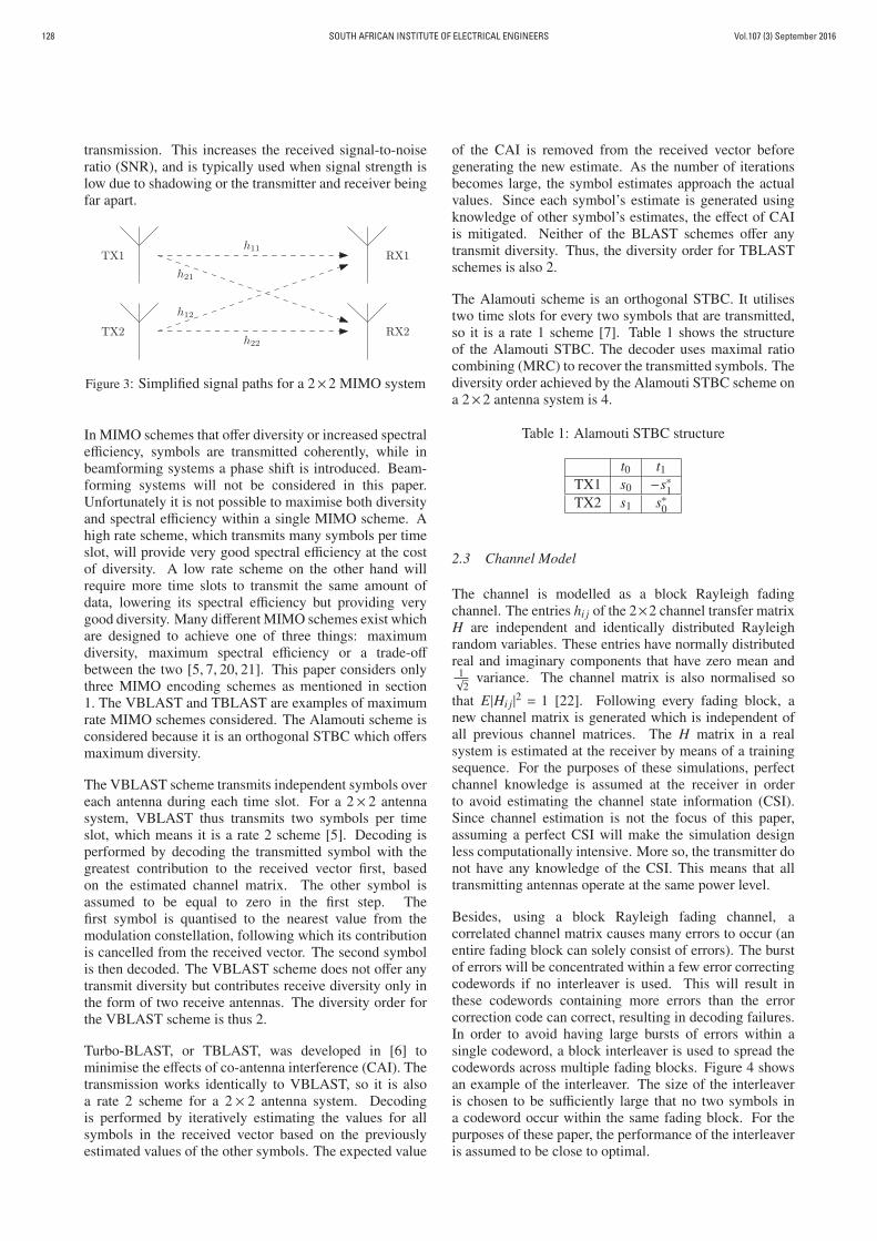
Vol.107 (3) September 2016SOUTH AFRICAN INSTITUTE OF ELECTRICAL ENGINEERS128
transmission. This increases the received signal-to-noiseratio (SNR), and is typically used when signal strength islow due to shadowing or the transmitter and receiver beingfar apart.
TX1
TX2
RX1
RX2
h11
h21
h12
h22
Figure 3: Simplified signal paths for a 2×2 MIMO system
In MIMO schemes that offer diversity or increased spectralefficiency, symbols are transmitted coherently, while inbeamforming systems a phase shift is introduced. Beam-forming systems will not be considered in this paper.Unfortunately it is not possible to maximise both diversityand spectral efficiency within a single MIMO scheme. Ahigh rate scheme, which transmits many symbols per timeslot, will provide very good spectral efficiency at the costof diversity. A low rate scheme on the other hand willrequire more time slots to transmit the same amount ofdata, lowering its spectral efficiency but providing verygood diversity. Many different MIMO schemes exist whichare designed to achieve one of three things: maximumdiversity, maximum spectral efficiency or a trade-offbetween the two [5, 7, 20, 21]. This paper considers onlythree MIMO encoding schemes as mentioned in section1. The VBLAST and TBLAST are examples of maximumrate MIMO schemes considered. The Alamouti scheme isconsidered because it is an orthogonal STBC which offersmaximum diversity.
The VBLAST scheme transmits independent symbols overeach antenna during each time slot. For a 2× 2 antennasystem, VBLAST thus transmits two symbols per timeslot, which means it is a rate 2 scheme [5]. Decoding isperformed by decoding the transmitted symbol with thegreatest contribution to the received vector first, basedon the estimated channel matrix. The other symbol isassumed to be equal to zero in the first step. Thefirst symbol is quantised to the nearest value from themodulation constellation, following which its contributionis cancelled from the received vector. The second symbolis then decoded. The VBLAST scheme does not offer anytransmit diversity but contributes receive diversity only inthe form of two receive antennas. The diversity order forthe VBLAST scheme is thus 2.
Turbo-BLAST, or TBLAST, was developed in [6] tominimise the effects of co-antenna interference (CAI). Thetransmission works identically to VBLAST, so it is alsoa rate 2 scheme for a 2 × 2 antenna system. Decodingis performed by iteratively estimating the values for allsymbols in the received vector based on the previouslyestimated values of the other symbols. The expected value
of the CAI is removed from the received vector beforegenerating the new estimate. As the number of iterationsbecomes large, the symbol estimates approach the actualvalues. Since each symbol’s estimate is generated usingknowledge of other symbol’s estimates, the effect of CAIis mitigated. Neither of the BLAST schemes offer anytransmit diversity. Thus, the diversity order for TBLASTschemes is also 2.
The Alamouti scheme is an orthogonal STBC. It utilisestwo time slots for every two symbols that are transmitted,so it is a rate 1 scheme [7]. Table 1 shows the structureof the Alamouti STBC. The decoder uses maximal ratiocombining (MRC) to recover the transmitted symbols. Thediversity order achieved by the Alamouti STBC scheme ona 2×2 antenna system is 4.
Table 1: Alamouti STBC structure
t0 t1TX1 s0 −s∗1TX2 s1 s∗0
2.3 Channel Model
The channel is modelled as a block Rayleigh fadingchannel. The entries hi j of the 2×2 channel transfer matrixH are independent and identically distributed Rayleighrandom variables. These entries have normally distributedreal and imaginary components that have zero mean and
1√2
variance. The channel matrix is also normalised so
that E|Hi j|2 = 1 [22]. Following every fading block, anew channel matrix is generated which is independent ofall previous channel matrices. The H matrix in a realsystem is estimated at the receiver by means of a trainingsequence. For the purposes of these simulations, perfectchannel knowledge is assumed at the receiver in orderto avoid estimating the channel state information (CSI).Since channel estimation is not the focus of this paper,assuming a perfect CSI will make the simulation designless computationally intensive. More so, the transmitter donot have any knowledge of the CSI. This means that alltransmitting antennas operate at the same power level.
Besides, using a block Rayleigh fading channel, acorrelated channel matrix causes many errors to occur (anentire fading block can solely consist of errors). The burstof errors will be concentrated within a few error correctingcodewords if no interleaver is used. This will result inthese codewords containing more errors than the errorcorrection code can correct, resulting in decoding failures.In order to avoid having large bursts of errors within asingle codeword, a block interleaver is used to spread thecodewords across multiple fading blocks. Figure 4 showsan example of the interleaver. The size of the interleaveris chosen to be sufficiently large that no two symbols ina codeword occur within the same fading block. For thepurposes of these paper, the performance of the interleaveris assumed to be close to optimal.

Vol.107 (3) September 2016 SOUTH AFRICAN INSTITUTE OF ELECTRICAL ENGINEERS 129
Codeword 1
Codeword 2
Codeword 3
Transmission order
Codeword Length
Blockfadelength
Figure 4: Interleaver structure showing ordering oftransmitted symbols
The 2×1 received signal from the channel output (receivedvector r) is given as:
r =Hx+n, (1)
where H is the 2 × 2 channel matrix, x is the 2 × 1transmitted vector, and n is the 2 × 1 noise vector. Thechannel matrix H represents the individual paths betweenantenna pairs such that:
H =[h11 h12h21 h22
], (2)
where hi j is a complex value representing the magnitudeand phase shift of the path from transmitting antenna jto receiving antenna i. Objects such as walls reflect theradio waves travelling from the transmitter to the receiver,causing changes in phase and angle of arrival of the waves.The signal propagates along a slightly different path foreach antenna pair. Channel paths are thus of differentlengths and experience different levels of attenuation. Thechannel entries hi j are complex numbers indicating thephase and magnitude change introduced by each of thechannel paths. The exact values of the channel entries usedin simulations are determined by the channel model used.
3. RESULTS
The results are presented using simulations run inMATLAB. Feasibility of systems is determined bycomparing the symbol error rate of the systems across arange of signal to noise ratios. The MIMO configurationused has two transmitting and two receiving antennas(2 × 2). A Rayleigh fading channel is used as thismodels a rich scattering environment, as encountered inindoor and heavily built up environments [16]. Threedifferent MIMO schemes are simulated: one system withrate 1 and two systems with rate 2. The rate 1 schemeis the Alamouti scheme, which is an orthogonal STBCspecifically designed for 2 × 2 systems. The rate 2 schemesare the VBLAST and TBLAST schemes, which haveidentical transmission structures but differ in the decodingalgorithm as explained in section 2.2.
The system uses 16-QAM modulation. Reed-Solomonchannel coding [8] is used with a symbol size of four bitsso that each modulation symbol maps to a single codesymbol. To achieve the longest possible codewords giventhe size of the symbol space, the codeword length is n = 15.The message k assumes different sizes in order to performhigh and low rate simulations. Both hard and soft decisiondecoding are implemented. The hard decision decodingis implemented using the Berlekamp-Massey algorithm[9, 10]. Soft decision decoding is used since it can decodebeyond the conventional error correcting ability of the codeand is particularly suited to low rate codes [17]. TheGuruswami-Sudan algorithm [17] is used along with theKoetter-Vardy algorithm [13] for soft decision decoding.
The primary objective of this paper is to compare three2 × 2 MIMO systems with equal overall rate but withdifferent MIMO and RS error correcting code rates. Thedata generated in order to perform this comparison canalso be used to draw several other conclusions. Thissection is therefore structured as follows. In order tojustify the selection of code rates, section 3.1 evaluatesa range of rates using each of the MIMO schemes.The preferred high rate MIMO scheme is then selectedby comparing VBLAST and TBLAST in section 3.2.Section 3.3 analyses the impact of using soft decisiondecoding with various code rates over all three MIMOschemes. Finally, systems with equal overall rates arecompared in section 3.4, which addresses the aim of thepaper.
3.1 Optimal code rates
When performing comparisons between different ratecodes, it is important to keep the total energy transmittedper message symbol constant. Suppose the reference valueof the energy per symbol Es is based on an uncoded datastream. If an (n,k) code were used and each of the nsymbols were transmitted using Es energy, the total energyused to transmit the stream should be n
k times higher thanthe reference data stream. It should thus achieve lowererror rates than the reference stream not solely due to theerror correcting code, but also due to the higher SNR.Therefore, to use the error correcting codes it is necessaryto spread the energy from the reference message acrossall the codeword symbols to maintain a fair comparison.Each codeword symbol is therefore transmitted using k
n Esenergy. It is well known that low rate codes are capable ofcorrecting more errors than high rate codes. This, however,comes at the expense of reduced energy per codewordsymbol. Reduced energy per codeword symbol results inmore errors that need to be corrected, which counteractsthe error correcting improvement.
The fact that error correction codes offer a gain overuncoded systems indicates that the error correctingimprovement is greater than the energy reduction. This isnot true for all code rates though. Consider a trivial (15,1)code. The same symbol is transmitted 15 times with anenergy of 1
15 Es. For all practical purposes this is equivalentto transmitting a single symbol with energy Es, which is

Vol.107 (3) September 2016SOUTH AFRICAN INSTITUTE OF ELECTRICAL ENGINEERS130
the same as an uncoded system. There is therefore a pointat which decreasing the code rate is not going to provideany further improvements in error rate.
The error rate curves for RS codes of length 15 with HDdecoding in a SISO AWGN channel are shown in figure 5.The (15,9) RS code offers the best performance, but the(15,11) and (15,7) codes offer comparable performance atan SER of 10−4. The (15,5) code performs 0.9 dB worsethan the (15,9) code. This is not the case for all channelmodels as we demonstrate in subsequent sections.
6 8 10 12 14 16
10−4
10−3
10−2
10−1
SNR (dB)
Sym
bol E
rror
Rate
(15,1), HD
(15,3), HD
(15,5), HD
(15,7), HD
(15,9), HD
(15,11), HD
(15,13), HD
Figure 5: Comparison of code rates in a SISO AWGNchannel
6 8 10 12 14 16
10−4
10−3
10−2
10−1
SNR (dB)
Sym
bol E
rror
Rate
(15,1), HD
(15,3), HD
(15,5), HD
(15,7), HD
(15,9), HD
(15,11), HD
(15,13), HD
Figure 6: Comparison of code rates in a SISO Rayleighfading channel
For practical purposes, the SISO equivalent of the Rayleighfading channel used in this paper is an AWGN channel.The Rayleigh fading coefficient can be thought of as ascalar H which is multiplied with the received vector toeffect a change in magnitude and phase. Since the MIMOchannel model requires that E
[|Hi j|2
]= 1, the magnitude
of H in the SISO case is unity. The transmitted vector thusonly experiences a phase shift, but since perfect channelstate information is assumed at the receiver, this phase shiftis reversed at the receiver. The only effect that the channelhas is thus to rotate the white Gaussian noise, which has nosignificant effect. To verify this, Figure 6 shows the error
rate curves for a SISO block Rayleigh fading channel. Asanticipated, the results are identical to Figure 5, with (15,9)RS codes exhibiting the best performance.
On the other hand, MIMO channels exhibit somewhatdifferent characteristics. Figures 7, 8 and 9 respectivelyshow the results of comparing various RS code rates.
6 7 8 9 10 11 12 13 14
10−4
10−3
10−2
10−1
SNR (dB)
Sym
bol E
rror
Rate
(15,1), HD
(15,3), HD
(15,5), HD
(15,7), HD
(15,9), HD
(15,11), HD
(15,13), HD
Figure 7: Comparison of code rates in an Alamouti MIMOsystem
Using the Alamouti scheme, it is evident from Figure 7 thatthe (15,9) RS code achieves a SER of 10−4 at the lowestSNR. It outperforms the (15,11) and (15,7) codes by 0.18dB and 0.27 dB respectively. The (15,5) code performs 1dB worse than the best performing code ((15,9)). Theseresults are very similar to the results for a SISO AWGNchannel because the (15,9) code outperforms the othercodes by the same margins. The Alamouti scheme is thuseffectively eliminating the effect of the multipath fading,making the MIMO channel behave in the same way as aSISO AWGN channel.
8 10 12 14 16 18 20 22 24 26
10−4
10−3
10−2
10−1
SNR (dB)
Sym
bol E
rror
Rate
(15,1), HD
(15,3), HD
(15,5), HD
(15,7), HD
(15,9), HD
(15,11), HD
(15,13), HD
Figure 8: Comparison of code rates in a VBLAST MIMOsystem
The results are somewhat different when utilising theVBLAST scheme as depicted in Figure 8. In contrast tothe SISO and Alamouti results, the (15,5) code offers thebest performance at an SER of 10−4, closely followed by

Vol.107 (3) September 2016 SOUTH AFRICAN INSTITUTE OF ELECTRICAL ENGINEERS 131
the (15,7) code. The (15,9) code performs 1.4 dB worsethan the (15,5) code. This phenomenon is explained byconsidering the propagation of symbol errors within theVBLAST structure. When the first symbol in the VBLASTdecoding process produces an error, the wrong value isused in the cancelling process. The second symbol isthus decoded using erroneous information, dramaticallyincreasing the error probability of the second symbol aswell. This interdependence of symbols results in additionalerrors, requiring greater error correcting capability fromthe channel code. Although the interleaver minimises theimpact of error propagation on single codewords, the effectremains noticeable due to cross-propagation of errors fromdifferent codewords.
8 10 12 14 16 18 20 22 24 26
10−4
10−3
10−2
10−1
SNR (dB)
Sym
bol E
rror
Rate
(15,1), HD
(15,3), HD
(15,5), HD
(15,7), HD
(15,9), HD
(15,11), HD
(15,13), HD
Figure 9: Comparison of code rates in a TBLAST MIMOsystem
TBLAST exhibits similar properties to VBLAST, in thatthe optimal code rate is lower than that for the SISOAWGN channel. Once again the (15,5) code performs thebest, achieving an SER of 10−4 at 18.8 dB. The (15,3)and (15,7) codes offer the next best performance at around19.5 dB. The (15,9) code performs 3.3 dB worse than thebest performing code. An interesting difference betweenTBLAST and VBLAST is that an error floor is evidentwhen using TBLAST in conjunction with higher coderates. The (15,11) code exhibits an error floor at an SER of10−3.44 while the error floor for the (15,13) code is as highas 10−2.37. Lower rate codes would also experience errorfloors, although these occur below the simulation SERcut-off of 10−4. Even when there is no noise present, thereis thus a limit to the achievable error rate for each code rate.Errors under noise free conditions were found to occurwhen the channel matrix had strong spatial correlation.Due to the channel matrix being generated as a set of fourindependent and identically distributed Rayleigh randomvariables, there is some probability that the channel for anygiven fading block is spatially correlated.
These bad channel states often resulted in both symbolstreams producing errors. Although the interleaver ensuresthat no fading block allows more than one symbol percodeword, the errors caused by multiple poor channelsoverwhelmed the error correcting capability of the RScodes in some cases. The probability of a codeword
containing enough poor fading blocks to overwhelm theerror correcting capability decreases for low rate codes,resulting in a lower error floor.
In order to establish whether bad channels affect bothsymbol streams, simulations were run using an interleaverwhich transmitted two symbols from the same codewordin each time slot. Figure 10 shows the error floorsfor the (15,13), (15,11) and (15,9) codes at an SER of10−1.93, 10−2.75 and 10−3.35 respectively. These floors aresignificantly higher, indicating that the error correctionability of the code is more easily overwhelmed due to bothsymbols in a time slot becoming corrupted. If only onesymbol was being corrupted the error floor would be lowerthan in Figure 9, since the likelihood of
⌊n−k
2
⌋+ 1 poor
fading blocks per 8 blocks is lower than the likelihood ofthe same number of poor blocks per 15 blocks.
10 15 20 25 30
10−4
10−3
10−2
10−1
SNR (dB)
Sym
bol E
rror
Rate
(15,1), HD
(15,3), HD
(15,5), HD
(15,7), HD
(15,9), HD
(15,11), HD
(15,13), HD
Figure 10: Error floors using TBLAST while transmittingsymbols from the same codeword in each time slot
The absence of an error floor in the VBLAST curvesis indicative of the manner in which errors are caused.In some cases, an incorrect error in the first decodedsymbol will result in the second decoded symbol also beingincorrect. If this propagating error was due to spatialcorrelation, the errors would be present even at very highSNRs, resulting in an error floor. Since no error floor isevident even for high rate RS codes, the propagating errorsare therefore induced by noise. A correlated channel couldpotentially aggravate the effect of noise for the seconddecoded symbol, but due to the ordering of detection it hasa minimal impact on the first symbol.
Based on the results in this section, the best error rates areachieved using (15,5) RS codes with the VBLAST andTBLAST schemes and (15,9) codes with the Alamoutischeme. The optimal rates are not expected to bechanged by using soft decision decoding, despite lowerrates experiencing a greater SD gain. For VBLAST andTBLAST, the (15,3) code performs approximately 0.8 dBworse than the (15,5) code. Considering the soft-decisiongains found in section 3.3, the (15,3) code is unlikely to beoptimal even with SD decoding. When using the Alamoutischeme, the gap to the next lowest rate code is only 0.3 dB.Extrapolating the results in section 3.3, once again suggest

Vol.107 (3) September 2016SOUTH AFRICAN INSTITUTE OF ELECTRICAL ENGINEERS132
that the (15,7) code will at best match the performance ofthe (15,9) code. A natural selection for two codes wherethe ratio of rates is 2 is thus the (15,5) and (15,9) codes,with (15,10) codes being used with soft-decision decoding.
3.2 VBLAST vs TBLAST
The two BLAST based schemes use an identicaltransmission structure, that is, transmitting independentstreams of information over each antenna. TBLAST offersbetter performance on systems with many transmit andreceive antennas as shown in [6]. This is due to improvedhandling of CAI. On systems with few antennas, such asthe 2× 2 MIMO system used in this paper, CAI does notconstitute as large a fraction of the total received power.VBLAST is therefore less likely to erroneously decode thefirst symbol for systems with few antennas than systemswith many antennas.
6 8 10 12 14 16 18
10−4
10−3
10−2
10−1
100
SNR (dB)
Sym
bol E
rror
Rate
(15,5) VBLAST, HD
(15,9) VBLAST, HD
(15,5) TBLAST, HD
(15,9) TBLAST, HD
Figure 11: Comparison of VBLAST and TBLAST using a2×2 MIMO system and the B-M decoding algorithm
10 12 14 16 18 20
10−4
10−3
10−2
10−1
SNR (dB)
Sym
bol E
rror
Rate
(15,5) VBLAST, SD
(15,9) VBLAST, SD
(15,5) TBLAST, SD
(15,9) TBLAST, SD
Figure 12: Comparison of VBLAST and TBLAST using a2×2 MIMO system and the KV decoding algorithm
Figures 11 and 12 show the performance of the twoBLAST based schemes using hard and soft decisiondecoding respectively. It is evident that VBLAST andTBLAST offer similar performance, but VBLAST offersmarginally better performance at an error rate of 10−4 forall four rate/decoding combinations. With hard-decision
decoding VBLAST outperforms TBLAST by 0.3 dB and1.3 dB for the (15,5) and (15,9) codes respectively.With SD decoding, VBLAST outperforms TBLAST by0.1 dB and 0.4 dB for the low and high rate codes.The difference in margins is attributable to the channelinduced errors experienced by TBLAST as discussed inthe previous section. As a result, the increased errorcorrection capability provides a more significant benefitto TBLAST. Although TBLAST may offer a significantgain for large antenna systems, this performance increaseis not evident when there are only two transmitting andreceiving antennas. This is explained by considering theenergy contribution of the desired symbol and the CAI.With two transmitting antennas, the expected CAI energyis equal to the expected symbol energy, resulting in asignal-to-CAI ratio (SCR) of 0 dB. With 16 transmittingantennas, the expected CAI energy is 15 times greater thanthe expected symbol energy, which is an SCR of −11.8dB. It is clear that handling of CAI becomes significantlymore important when a large number of antennas arepresent. The technique of ordering symbol decoding bypost-detection SNR as used in VBLAST thus providesmore of a benefit than iteratively estimating the CAI. It isalso shown in section 3.1 that TBLAST is more likely thanVBLAST to cause error propagation when the channel isspatially correlated.
3.3 Soft decision decoding gain
Soft-decision (SD) RS decoding offers some improvementin error rate performance at the expense of significantlyincreased complexity. Analysing the complexity perfor-mance trade-off is not the objective of this paper, butthe performance increase is quantified in this section.The asymptotic error correcting capability of the GSalgorithm used by KV is n − 1 −
⌊√(k−1)n
⌋, compared
to a hard-decision bound of⌊
n−k2
⌋. The benefit of
using soft-decision decoding thus increases as the coderate decreases. The KV algorithm offers performanceexceeding the bound of the GS algorithm. The errorcorrecting capability can however not be easily quantified,since some symbol reliability patterns allow more errors tobe corrected than others.
The soft-decision gain obtained using the KV algorithmis investigated for all three MIMO schemes using (15,5),(15,9) and (15,10) RS codes. Since a (15,10) code hast = 2 while a (15,9) code has t = 3, the lower hard-decisionperformance of the former code should result in a largersoft-decision gain as the SD decoder is not affected by theodd number of parity symbols. Additionally, it is expectedthat the (15,5) code will exhibit a larger SD gain thanthe higher rate codes due to the increased error correctingcapability.
Figure 13 shows error rate performance for the threecode rates over an Alamouti scheme with hard andsoft decoding. This demonstrates the effect of usingsoft-decision decoding on RS codes when there are an oddnumber of parity symbols. At a SER of 10−4, the (15,9)

Vol.107 (3) September 2016 SOUTH AFRICAN INSTITUTE OF ELECTRICAL ENGINEERS 133
code exhibits a soft-decision gain of 0.9 dB, compared to1.3 dB for the (15,10) code, implying a difference of 0.4dB. It can thus be concluded that the soft-decision decoderdoes not suffer a significant penalty from an odd numberof parity symbols as compared to a hard-decision decoder.
To analyse the effect of code rate on soft-decision gain, itis thus not practical to include codes with an odd (n− k).This analysis is therefore performed using only the (15,5)and (15,9) RS codes. Figures 13, 14, and 15 show theperformance of the two codes in conjunction with theAlamouti, VBLAST and TBLAST schemes respectively.The soft-decision gain for all combinations of code ratesand MIMO schemes is summarised in table 2.
5 6 7 8 9 10 11 12 13
10−4
10−3
10−2
10−1
SNR (dB)
Sym
bol E
rror
Rate
(15,5) Alamouti, SD
(15,9) Alamouti, SD
(15,10) Alamouti, SD
(15,5) Alamouti, HD
(15,9) Alamouti, HD
(15,10) Alamouti, HD
Figure 13: Comparison of soft and hard decision RSdecoding with the Alamouti scheme
10 12 14 16 18 20 22
10−4
10−3
10−2
10−1
SNR (dB)
Sym
bol E
rror
Rate
(15,5) TBLAST, SD
(15,9) TBLAST, SD
(15,5) TBLAST, HD
(15,9) TBLAST, HD
Figure 14: Comparison of soft and hard decision RSdecoding with the VBLAST scheme
Table 2: Summary of soft-decision gains in dB at SER = 10−4
(15,5) (15,9) DifferenceAlamouti 1.4 0.9 0.5VBLAST 1.3 0.4 0.9TBLAST 1.5 1.2 0.3
On average, the soft-decision gain for the (15,5) code is0.7 dB higher than for the (15,9) code. This is attributable
10 12 14 16 18 20 22
10−4
10−3
10−2
10−1
SNR (dB)
Sym
bol E
rror
Rate
(15,5) TBLAST, SD
(15,9) TBLAST, SD
(15,5) TBLAST, HD
(15,9) TBLAST, HD
Figure 15: Comparison of soft and hard decision RSdecoding with the TBLAST scheme
to the improved error correcting capability of soft-decisiondecoding for low rate codes. The three MIMO schemesexhibit approximately similar soft-decision gain for thelow rate code. For both high and low rate code, VBLASTexperiences the lowest SD gain compared to the AlamoutiSTBC and TBLAST schemes. This is due to errorpropagation in VBLAST increasing the likelihood of theerror correcting capability being exceeded. Additionally,this indicates that VBLAST is generating less accuratesoft information in comparison to the Alamouti STBC andTBLAST schemes. If an error occurs in the first decodedsymbol, the error propagates to the second symbol. Bothsymbols have errors and are likely to have low reliability,but this does not necessarily hamper the performance ofthe SD decoder. However, the scenario where the firstsymbol is decoded correctly but the second symbol isdecoded incorrectly can cause problems. The feedbackmechanism which generates the soft information for thefirst symbol will thus back-propagate the error, resultingin the first (correct) symbol having poor reliability. Thesoft decision decoder is then prone to ignore the correctsymbol, potentially favouring some error symbols in itsplace. These properties result in there being slightly lessbenefit to using soft-decision decoding in conjunction withVBLAST.
3.4 Transmit diversity vs code rate
The primary objective of this paper is to investigate thefeasibility of using low rate codes as an alternative todiversity. VBLAST is used as the rate 2 MIMO scheme,as it is shown in section 3.2 to offer better performancethan TBLAST. The VBLAST scheme is paired with a(15,5) RS code and is compared to the Alamouti STBCwith (15,10) RS coding, keeping the overall rate of thetwo systems constant. These code rates were also shownin section 3.1 to be optimal or close to optimal for eachMIMO scheme. Soft-decision RS decoding is used withboth systems. Figure 16 shows a comparison betweenthese two schemes using the KV decoding algorithm.
The high diversity system outperforms the low diversity

Vol.107 (3) September 2016SOUTH AFRICAN INSTITUTE OF ELECTRICAL ENGINEERS134
8 10 12 14 16 18
10−4
10−3
10−2
10−1
SNR (dB)
Sym
bol E
rror
Rate
(15,5) VBLAST, SD
(15,10) Alamouti, SD
Figure 16: Comparison of MIMO systems with equaloverall rate
system by 6.2 dB at a symbol error rate of 10−4. Thisindicates a very large SER gain, implying that the highdiversity system can achieve the same error rates as thelow diversity system while using about four times lesspower. Thus, low rate channel codes are thus not afeasible alternative to transmit diversity in the MIMOsystems which were evaluated. It can be concluded fromthis result that increasing transmit diversity is significantlymore effective than decreasing code rate for the systemsimulated. Although this conclusion can only be drawnunder the conditions of this simulation, the magnitudeof the margin suggests that similar results are likely tobe achieved using different channel models and MIMOschemes. The mechanism by which the high rate systemachieves such good performance is that it reduces thenumber of symbol errors in the received vector before itis passed to the RS decoder. The number of pre-decodingsymbol errors eliminated by high diversity exceeds theincrease in error correcting capability of the low rate codeby a significant margin.
4. CONCLUSION
In this paper, the performance of three 2 × 2 MIMOsystems have been studied for different channel coderates. Given the computer simulation results, three primaryconclusions can be drawn from this study. Firstly, lowrate channel codes are not a feasible alternative to transmitdiversity in a 2×2 MIMO systems. Using error correctionas an alternative to diversity is thus not a practicalsolution. Secondly, while TBLAST may offer significantperformance improvements over VBLAST in systems witha large number of antennas, the two schemes performvirtually identically for a 2×2 system. Finally, there is noappreciable difference in soft-decision gain between lowdiversity and high diversity 2×2 MIMO schemes.
ACKNOWLEDGEMENT
The financial assistance of the National ResearchFoundation (NRF) of South Africa towards this researchis hereby acknowledged. Opinions expressed and
conclusions arrived at, are those of the authors and arenot necessarily to be attributed to the NRF. The financialsupport of the Centre for Telecommunication Access andServices (CeTAS), the University of the Witwatersrand,Johannesburg, South Africa is also acknowledged.
REFERENCES
[1] ETSI, “3GPP TS 36.213 Evolved Universal Ter-restrial Radio Access (E-UTRA); Physical layerprocedures,” www.etsi.org, Tech. Rep., 2014.
[2] “IEEE Standard for Information technology – Localand metropolitan area networks – Specific require-ments – Part 11: Wireless LAN Medium AccessControl (MAC) and Physical Layer (PHY) Speci-fications Amendment 5: Enhancements for HigherThroughput,” IEEE Std 802.11n-2009 (Amendmentto IEEE Std 802.11-2007 as amended by IEEE Std802.11k-2008, IEEE Std 802.11r-2008, IEEE Std802.11y-2008, and IEEE Std 802.11w-2009), pp.1–565, Oct 2009.
[3] “IEEE Standard for Information technology –Telecommunications and information exchange be-tween systems. Local and metropolitan area networks– Specific requirements – Part 11: Wireless LANMedium Access Control (MAC) and Physical Layer(PHY) Specifications–Amendment 4: Enhancementsfor Very High Throughput for Operation in Bands be-low 6 GHz.” IEEE Std 802.11ac-2013 (Amendmentto IEEE Std 802.11-2012, as amended by IEEE Std802.11ae-2012, IEEE Std 802.11aa-2012, and IEEEStd 802.11ad-2012), pp. 1–425, Dec 2013.
[4] L. A. M. Guzman, “A Study on MIMOMobile-To-Mobile Wireless Fading ChannelModels ,” Master’s thesis, School of Engineeringand Physical Sciences, Heriot Watt University , June2008.
[5] P. Wolniansky, G. Foschini, G. Golden, and R. Valen-zuela, “V-BLAST: an architecture for realizing veryhigh data rates over the rich-scattering wirelesschannel,” in Signals, Systems, and Electronics, 1998.ISSSE 98. 1998 URSI International Symposium on,Sep. 1998, pp. 295–300.
[6] M. Sellathurai and S. Haykin, “TURBO-BLAST forhigh-speed wireless communications,” in WirelessCommunications and Networking Confernce, 2000.WCNC. 2000 IEEE, vol. 1, 2000, pp. 315–320 vol.1.
[7] S. Alamouti, “A simple transmit diversity techniquefor wireless communications,” Selected Areas inCommunications, IEEE Journal on, vol. 16, no. 8,pp. 1451–1458, Oct 1998.
[8] I. G. Reed and G. Solomon, “Polynomial codes overcertain finite fields,” J. Soc.Ind. Appl. Maths., pp.8:300–304, June 1960.
[9] E. R. Berlekamp, Algebraic Coding Theory. NewYork: McGraw-Hill, Inc., 1968.

Vol.107 (3) September 2016 SOUTH AFRICAN INSTITUTE OF ELECTRICAL ENGINEERS 135
[10] J. Massey, “Shift-register synthesis and bch decod-ing,” Information Theory, IEEE Transactions on,vol. 15, no. 1, pp. 122–127, Jan 1969.
[11] Y. Sugiyama, M. Kasahara, S. Hirasawa, andT. Namekawa, “A method for solving key equationfor decoding goppa codes,” Information and Control,vol. 27, no. 1, pp. 87 – 99, 1975.
[12] L. R. Welch and E. R. Berlekamp, “Error correctionfor algebraic block codes,” Patent US 4 633 470, Dec30, 1986.
[13] R. Koetter and A. Vardy, “Algebraic soft-decisiondecoding of Reed-Solomon codes,” InformationTheory, IEEE Transactions on, vol. 49, no. 11, pp.2809–2825, Nov 2003.
[14] J. Jiang and K. Narayanan, “Iterative Soft-InputSoft-Output Decoding of Reed amp; #8211;SolomonCodes by Adapting the Parity-Check Matrix,”Information Theory, IEEE Transactions on, vol. 52,no. 8, pp. 3746–3756, Aug 2006.
[15] O. Ur-rehman and N. Zivic, “Soft decision iterativeerror and erasure decoder for Reed #8211;Solomoncodes,” Communications, IET, vol. 8, no. 16, pp.2863–2870, 2014.
[16] W. C. Jakes and D. C. Cox, Eds., Microwave MobileCommunications. Wiley-IEEE Press, 1994.
[17] V. Guruswami and M. Sudan, “Improved decodingof Reed-Solomon and algebraic-geometric codes,” inFoundations of Computer Science, 1998. Proceed-ings. 39th Annual Symposium on, Nov 1998, pp.28–37.
[18] O. Ogundile and D. Versfeld, “Improved relia-bility information for rectangular 16-QAM overflat rayleigh fading channels,” in ComputationalScience and Engineering (CSE), 2014 IEEE 17thInternational Conference on, Dec 2014, pp. 345–349.
[19] L. Godara, “Application of antenna arrays tomobile communications. II. Beam-forming anddirection-of-arrival considerations,” Proceedings ofthe IEEE, vol. 85, no. 8, pp. 1195–1245, Aug 1997.
[20] C. Han, X. Zhang, and Y. Chen, “A novel full densityQSTBC scheme with low complexity,” in Image andSignal Processing (CISP), 2013 6th InternationalCongress on, vol. 03, Dec 2013, pp. 1478–1482.
[21] H. Lee, “Robust full-diversity full-ratequasi-orthogonal STBC for four transmit antennas,”Electronics Letters, vol. 45, no. 20, pp. 1044–1045,September 2009.
[22] G. J. Foschini and M. J. Gans, “On limits ofwireless communications in a fading environmentwhen using multiple antennas,” Wireless PersonalCommunications, vol. 6, pp. 311–335, 1998.

Vol.107 (3) September 2016SOUTH AFRICAN INSTITUTE OF ELECTRICAL ENGINEERS136
INTELLIGENT WEATHER AWARENESS TECHNIQUE FOR MITIGATING PROPAGATION IMPAIRMENT AT SHF AND EHF SATELLITE NETWORK SYSTEM IN A TROPICAL CLIMATE. I.A. Adegbindin*, P.A. Owolawi** and M.O. Odhiambo*** * Dept. of Electrical and Mining Engineering, University of South Africa, Private Bag X6, 1710 Florida Pretoria, South Africa ** Dept. of Electrical Engineering, Mangosuthu University of Technology, P. O. Box 12363, Jacob, 4026 Durban, South Africa *** Dept. of Process Control & Computer System, Vaal University of Technology, Private Bag X021, Vanderbijlpark 1911, South Africa Abstract: This paper presents an Intelligent Weather Awareness Technique (IWT) based on fuzzy logic to achieve optimum signal quality when the impact of weather attenuations become manifest in Earth-satellite link. An adaptive measure of a decision support system is adopted using the point rainfall rate to predict rain-induced attenuation over three locations in the tropical region of Nigeria based on Moupfouma rain rate and attenuation model. In order to impact good Quality of Service (QoS) in the overall design of satellite communication networks, considerable efforts have to be made, such as the use of appropriate forward error correction codes, the choice of modulations and the range of uplink/downlink power controls. The IWT interacts with the input parameters to optimise the Signal to Noise Ratio (SNR) values while the input parameters are varying. The results show that in all three locations considered, a minimum fade margin of about 12 dB on the uplink and ~ 8 dB on the downlink may be allowed at the 99.5% availability for a worst case scenario at Ka-band. Analysis based on SNR and consumed power at the same weather conditions confirms the suitability of introduction of fuzzy logic for optimum availability of good QoS in a weather impaired satellite system. The overall results would provide tolerance margins needed for better QoS, especially during bad weather in the study locations. Key words: SNR, tropical weather, Intelligent Weather Awareness Technique, satellite network.
1. INTRODUCTION
Rain Induced Attenuation (RIA) is one of the major propagation impairments for radio wave propagation transmitting at high frequency bands above 10 GHz. At such frequency bands, rain attenuation absorbs and scatters radio waves, leading to signal degradation. The severity of the impairment becomes even more pronounced for frequencies as low as 7 GHz in the tropical and equatorial regions where intense rainfall events are common [1]. The significance of this event is usually observed at the receiving terminal by variations in the desired signal level. Precise technical knowledge of rain attenuation is therefore very important for designing and planning reliable satellite communication networks [2]. Common rain attenuation prediction methods require one-minute rain rate data at the location of study as recommended by the International Telecommunication Union (ITU), which is scarce globally with worst case in tropical regions [3]. The available rain data are usually of longer integration time like 5-minutes, 10-minutes, 30-minutes, hourly and daily data. These data are available at different weather or meteorological stations at different locations. Many investigators including Segal [4] proposed a conversion factor )(P for converting the raw data collected from measuring rain gauge to an equivalent 1-minute and note that P is defined as the percentage of exceedance with range over %03.0%001.0 P , in the
case of Rice Holmberg [5], a physical model was proposed based on cumulative distribution of rain rate. Two modes of methods were proposed: mode 1 deals with convective type of rain )( 1M while mode 2 deals with other types of rain )( 2M . The contribution of Kitami model [6] to integration time conversion is based on semi-empirical method by using the Kitami Institute of Technology(KIT) database which allow the variables such as latitude , longitude rain rate values at 0.01% and 0.001% of exceedences to be input to the general semi-empirical expression to yield 1-minute equivalent rain rate, and contribution of Moupfouma and Martins model [7] focus on three regions of climatic conditions which are tropic, temperate and sub-tropic and the model is more popular than previously mentioned model because of the inclusion of climatic parameters. The expressions and details of the above listed models and other related models are presented in the work by Owolawi [8] .The main purpose of all these models is to devise procedures to convert the available longer integration data to the required one-minute data. However, not all the models can fit into the tropical region based on the data from the temperate region used in developing some of the models. Invariably, some of the models do not give an accurate prediction of rain rate when applied to the tropical and equatorial regions [3]. Recent studies from the tropical region also show that rain rate distribution is better

Vol.107 (3) September 2016 SOUTH AFRICAN INSTITUTE OF ELECTRICAL ENGINEERS 137
described by a model which approximates a log-normal distribution of the low rain rates and gamma distribution of the high rain rate [3, 9]. Among the existing models, Moupfouma and Martins model (henceforth referred to as MM model) [7, 10] has been identified to fit into this factor [3, 11]. The model can be adopted for both tropical and temperate climates. Once the one-minute rain rate is obtained, the expected rain-induced attenuation that could be encountered along the satellite link can be estimated. Subsequently, the appropriate methods for mitigating the propagation impairment will be applied. Some of these include adaptive coding, antenna beam shaping, site diversity, and uplink power control [12]. Uplink power control has been identified as one of the most cost-effective attenuation mitigation techniques as it enhances link availability and performance [2, 12]. In tropical climates like Nigeria (with emphasis on some selected locations), rain is the predominant parameter among the hydrometeor; hence the effect of rain is majorly considered in this work. In this paper, we have adopted an Intelligent Weather Awareness Technique (IWT) to estimate the tolerance amount of SNR needed to achieve optimum signal quality when the impact of bad weather becomes manifest in Earth-satellite link. Results are presented in 3D forms as a function of propagation impairments for both propagation angle and rainfall rate at a Super High Frequency (SHF) and Extremely High Frequency (EHF) bands for three locations: Port Harcourt, Lagos and Akure. The data obtained were fed to the techniques adopted with a mechanism to better estimate satellite networking parameters such as link and queuing characteristics. The derived parameters would enable the Earth-satellite system to maintain QoS by adaptively adjusting satellite signal power, modulation, coding and data rate for unpredictable weather conditions in the region.
2. SITE, DATA AND METHODOLOGY In this section, we present a brief report on the characteristics of the locations considered, nature of the data used and methodology adopted based on this work. 2.1 Site and Data Three locations were considered for this work: Port Harcourt, Lagos and Akure. Each of these chosen locations represents different climatic regions of the country with some prominent record of the high amount of rainfall [3, 11]. Table 1 presents the climatic characteristics of the locations studied. In Nigeria, the coastal region received an annual average rainfall of about 3000 mm, while the arid/savannah region received an average accumulation of less than 1000 mm. The seasonal northward and southward
oscillatory movement of the InterTropical Discontinuity (ITD) largely dictates the weather pattern. Table 1: Climatic characteristics of the sites
Location Long (N), Lat (E)
Annual rainfall amount (mm/yr)
Climatic region
Port Harcourt (PH)
7.0, 4.2 2803 Coastal
Lagos 3.2, 6.3 1425 Semi-Coastal
Akure 8.3, 11. 58
1485 Rain Forest
The moist south-westerly winds from the South Atlantic Ocean, which is the source of moisture needed for rainfall and thunderstorms to occur, prevail over the country during the rainy season (April – October), while the north-easterly winds which raise and transport dust particles from the Sahara desert prevail all over the country during the dry/Harmattan period (November – March) [13]. Ten years (2002-2012) of archived rain rate data obtained from the Nigerian Meteorological Agency (NMA) for the three locations considered were processed to obtain the needed data of one-minute integration time. The network of rain gauges usually used by the NMA is comprised of a standard funnel of 127 mm in agreement with the World Meteorological Organization (WMO). Detailed descriptions are available in [3, 11] and not repeated here for the sake of brevity.
Methodology
(i) Estimation of rainfall rate of one-minute integration
time
The 10 years’ rain rate data collected from NMA were applied to the MM model [7]. The model can be expressed as [7]:
rRwrR
rRPz
01.0
01.04 exp1
10)( (1)
Where: r (mm/h) represents the rain rate exceeded for a fraction of time; R0.01 is the rain intensity exceeded during 0.01% of time in an average year (mm/h); and taking into account the shape of cumulative distribution of rain rate, parameter z is given by [7]:
01.001.0
01.0 1lnR
rR
Rrz (2)

Vol.107 (3) September 2016SOUTH AFRICAN INSTITUTE OF ELECTRICAL ENGINEERS138
The parameter w in Equation (1) governs the slope of rain rate cumulative distribution and depends on the local climatic conditions and geographical features, for tropical and sub-tropical settings [7]:
01.001.0
exp10ln4R
rR
w (3)
Where:
=1.066 and = 0.214.
The MM model requires three (3) parameters: λ, γ and R0.01. The first two parameters have been provided. To get the estimate value of R0.01, Moupfouma [10, 14] introduced a relationship whereby rain rate at different integration times is converted to one-minute equivalent at 0.01% exceedance of rain rate. The power law relationship of the model is given by [10]:
01.0minmin)1( RP (4)
Where:
061.0(min)987.0 (5) (5)
The equation (1) to (5) are valid within an integration time of 1min. < < 1 hr. Rain rate cumulative distribution of one-minute integration time is therefore obtained using Equations (1) to (5). (ii) Estimation of Rain-Induced Attenuation (RIA) The one-minute rain rate obtained based on Equations (1) to (5) is then applied to the Moupfouma rain attenuation model to estimate the RIA for these regions. The Moupfouma rain attenuation for terrestrial satellite links is given by [15]:
sm
s
Sp LLp
LRRpRudBA 36.0
25.001.0
01.0/1
38.0/)(
(6)
Where:
m = 1 + 1.4.10-4 f 1.76 Loge (Ls); f is frequency in GHz; and Ls is the slant path length in km. = 0 if Ls < 5 km, f < 25 GHz and 0.03 in all other cases. The values of u (p) for different regions of the world are stated in [16]. R0.01 and Rp are rainfall rates corresponding to rain rates of
0.01 and p percent of the time. The slant path length Ls, is given as follows:
s
sR
sRS L
HH
HHL
sin8500
2sin2
1
2
(7)
Where:
HR = 5.0 for 0o ≤ < 23o HR = 5.0 – 0.075 (-23), for ≥ 23o (8)
Where HS is the station height above the sea level, is a path elevation angle measured in degree and HR is height of the 0o Isotherm. The slant-path length, Ls, below the freezing rain height is obtained as follows:
sinSR
S
HHL
(km) (9)
The rain intensity, R0.01 (mm/h), exceeded for 0.01% of an average year obtained using Equation (5) is then obtained to deduce the specific attenuation, R (dB/km):
01.0kRR (10)
The values of k and α are dependent on the frequency, raindrop size, distribution, temperature, rain and polarization. Their values can be taken from [17]. (iii) Estimation of SNR The performance of a communication system is estimated based on the achievable signal-to-noise (SNR) at the receiver. The term SNR (in dB) refers to the estimation of signal strength as a function of signal degradation and background noise. In this work, SNR is analogous to Carrier-to-Noise ratio (C/N) in order to refer to receive carrier power. This power can be expressed as [18]:
2
0
4
lKTBLGGP
NC
NS
sys
rtt
(11)
Where
Pt = transmitting power (W); o = free-space wavelength (m); Gt and Gr are transmitting and receiving antenna gain respectively; K is the Boltzmann’s constant = 1.38x10⁻²³ J/K; B = bandwidth (Hz); Lsys is the system loss in ratio (unit less); and l is the range (m). T is the system effective noise temperature (K) which is defined as:

Vol.107 (3) September 2016 SOUTH AFRICAN INSTITUTE OF ELECTRICAL ENGINEERS 139
RA TTT (12)
Where:
AT is antenna noise temperature( external noise) and RT is the receiver noise temperature (internal noise) , both are in the unit of Kelvin. It must be noted that RT is often expressed as the receiver’s noise figure in dB. The KT rN
R 290).110( 10/ , where in this work the low-noise-amplifier (LNA) considered has a typical noise figure ranges dBtoNr 27.0 . Also the parameter Lsys is related to the atmospheric loss, polarizer loss and the total attenuation. Note that the relationship between the carrier frequency (in Gigahertz) and wavelength in meter is expressed as:
)(3.0)( GHzfm (13)
(iv) Method adopted for satellite application Since the concern of the paper if on satellite link, the transmitting side of the satellite is expressed as:
WGPEIRP TT , (14)
Where:
In the receiving side:
1,/
K
TTG
TGRA
T (15)
The terminologies EIRP and TG / are the equivalent isotropic power and figure of merit respectively. Considering equation (14) and (15), it is possible to re-write equation (11) as:
BLKLTGEIRP
NC
NS
SysF
/. (16)
To express the equation (16) in decibel, the equivalent expression is presented as [18]:
)./(60.228).(
)()(
)/(/)()(
HzKdBWHzdBB
dBLdBL
TdBTGdBWEIRPdBNC
NS
Sysf
(17)
Equation (17) is employed to estimate the signal to noise ratio of the system. To account for the increase in SNR to achieve better system performance, the method used by [19] has been used based on the aforementioned equations. (v) Theory of Fuzzy-Logic Controller Fuzzy logic controller is a rule driven system where the controller uses fuzzy logic procedures to simulate human thinking in dealing with a complex system. Fuzzy logic controller is a better tool in dealing with processes that are too complex to analyse, especially when the available sources of information are interpreted quantitatively and uncertain in classification. The same situation is observed when the transmitted signal are mixed with several impairments and employed multiple mitigation techniques are available. Fuzzy logic controller is a good candidate to handle this complex situation because it consists of four compositions which are fuzzifier, rule base, fuzzy interference and defuzzier. The application of fuzzy logic controller adopted in this paper is detailed the contribution of Amruta et al. [20], [21] and the modification is in the area of input variable and defuzzification where the gravity method is considered.
(vi) Optimisation of the Network The reliability of a network is quantified by the percentage of time that the link between transmitter and receiver can be established [22]. In order to achieve optimal performance along the link, we applied IWT through a Fuzzy logic algorithm. The schematic diagram for different stages in the intelligent technique is presented in Figure 1. The algorithm iteratively tuned the IWT based on the SNR values to adjust the weighted modulation to its optimal values. This can be achieved depending on the following: the weather conditions, pre-set tolerance margins and the configuration settings. According to Harb et al. [19], a better SNR can be achieved by considering the total attenuation that could be encountered along the space to Earth propagation link among other parameters needed for the intelligent control through Fuzzy logic algorithm. The intelligent control is therefore designed to easily check against each of the input signal parameters (frequency, adjusted SNR, propagation angles, size frame etc.) in the database and make comparison with the threshold value. In the first stage, the technique held input signal parameters such as frame size, propagation angle and frequency, and the estimated SNR values that were compared against the threshold level (-30 dB or 0 dBm) in a single database as adopted by Herb et al. [12, 19]. The expectation is that the result obtained should either be greater than or equal to the threshold level. Depending on the SNR values, the algorithm will decide to increase

Vol.107 (3) September 2016SOUTH AFRICAN INSTITUTE OF ELECTRICAL ENGINEERS140
relative power transmitted for a maximum limit of -30 dB (0 dBm), or to skip to the next step. In the next stage, SNR value will be checked among modulation and assigned coding values. If this value can be reached by using any of the modulation/coding selections as presented in Table 2, then the system will proceed to the final stage.
Figure 1: The schematic diagram of the intelligent technique for satellite system
Table 2: Modulation/Coding selection needed in order to
adjust SNR
Modulation
LDPC Code
Identifier
Es/N0(dB) Measured/ Estimate
Relative Power (dB)
Rain Rate (mm/hr)
QPSK 1/4 -1.93 -52 9.92 QPSK 1/3 1.72 -51 9.10 QPSK 2/5 1.81 -48 8.41 QPSK 1/2 2.23 -49 7.46 QPSK 3/5 2.66 -47 6.75 QPSK 2/3 3.07 -48 6.97 QPSK 3/4 3.49 -48 5.31 QPSK 4/5 3.88 -46 4.87 QPSK 5/6 4.17 -45 4.53 QPSK 8/9 4.91 -44 3.87 8PSK 3/5 4.17 -41 4.32 8PSK 2/3 4.83 -43 3.60 8PSK 3/4 5.61 -41 2.82 8PSK 5/6 6.76 -40 2.01 8PSK 8/9 7.64 -39 1.32 16PSK 2/3 5.94 -42 2.21 16PSK 3/4 6.67 -38 1.56 16PSK 4/5 7.21 -40 1.15 16PSK 5/6 7.61 -36 0.88 16PSK 8/9 8.60 -34 0.32
In the final stage, the technique will check among different SNR achieved outputs and make decisions based on the intelligent controller according to available parameters and necessary requirements. The given feedback will keep interchanging until a suitable value and optimum level are reached. Thus, this system can also change data rate, frame size, and frequency in order to adaptively adjust SNR by transmission rate in cases such as unpredicted bad weather conditions, by using Refresh Duration that is located in the first stage. The general expression that incorporates the transmission rate with respect to symbol energy-to-noise power density is presented in [18]:
)(| dBRNC
NE
sdBO
s (18)
Where:
sR is a transmission rate measured in symbols per
second and O
s
NE
determine the bit error rate of
transmission scheme and the characteristic of a satellite
link can be estimated based on the set value of O
s
NE
that
will guarantee a sufficient low bit error rate. 2.2 Propagation Experimental Scenario As measurements were not available for all sites, it was not possible to draw countrywide conclusions. Nevertheless, available data obtained from one of the sites, Akure, can allow for a point-wise comparison. Propagation campaign over an Earth-space path at Ku-band frequency of 12.245 GHz has been carried out in the year 2012 at the Department of Physics Federal University of Technology, in Akure, Nigeria. The Ku-band modulated signal was received by a 90cm offset parabolic dish, at an elevation angle of 53.2o to the down converter and the beacon receiver. The down converted Ku-band signal from EUTELSAT W4/W7 was then fed to a digital satellite meter and a spectrum analyzer for signal level monitoring and logging into a computer unit. Detailed characteristics of the setup link are reported on the work of [23]. Comparison between measured attenuation, the predicted and the ITU model is presented in Figure 2. A strong correlation could be seen between the measured and the predicted value, particularly at lower time percentages. However, values obtained based on the ITU model overestimates the rain-induced attenuation in this locality. This is evident at 0.01% unavailability of time where measured attenuation was 7.1 dB while the predicted attenuation is about 8.3 dB, yielding a relative error of
Transmitted Power
Meteorological Parameters
Power
Frequency
Type Modulatio
n
Increase Power
SNR
Feedback
Atmospheric Losses
(Attenuation inclusive)
Hidden Layers
Other losses SNR

Vol.107 (3) September 2016 SOUTH AFRICAN INSTITUTE OF ELECTRICAL ENGINEERS 141
about 16%. The relative error was obtained from the dB values based on the recommendation of [24].
Figure 2: Comparison between the measured and predicted signal attenuation in 2012
3. RESULTS AND DISCUSSION
3.1 Propagation Channel Influence The methodology necessary to design the physical layer of satellite communication systems, especially at Ku-band, relies on the implementation of a propagation margin to take into account rain attenuation. The link budgets are actually closed by finding solutions to a worst case scenario. The worst case is chosen for an instance percentage of the whole coverage (between 90% and 95%) on the one hand with respect to attenuation, and on the other hand with respect to carrier-to-interference ratio. It corresponds generally to both edges of coverage and low elevation. A performance assessment for the worst case scenario over a typical location among the study locations is considered (Lagos, Nigeria) for the corresponding (i) availability (or outage time), and (ii) evaluation of the system capacity or throughput. Figures 3 (a and b) show predicted cumulative distribution function (CDF) of total impairment performed with the MM model at Ka-band downlink and uplink frequency respectively, over different elevation angles, for a typical station in Ikeja, Lagos, a semi-coastal locality of Nigeria with a worst case with respect to attenuation. In order to affirm the safety margin of a system which is a function of reliability /availability, the desire total hours of outages must be established. Conventionally, the reliability/availability of a system ranges between 99.5 % (44 hours allowed outages) to 99.9% (0.88 hours of allowed outages). In this work we adopted 99.5% of reliability. Therefore, fade margins of about 12 dB on the uplink and of 8 dB on the downlink may allow the 99.5% availability requirement to be fulfilled good QoS at Ka-band for Lagos coverage. However, for Q-band frequencies needed for a future network, at the same target availability in a conventional system design, several tens of dBs would be needed to be compensated with a static margin, which is not possible
due to technology limitations, leading to low availability only. Figure 4 shows a typical Q-band uplink frequency for total impairments for Lagos, Nigeria. The same trend could be observed in the other locations, although with different compensation margins.
(a)
(b)
Figure 3: A typical prediction of total attenuation at Ka-band (a) downlink and (b) uplink frequency for Lagos
Figure 4: A typical prediction of total attenuation at Q-band uplink
3.2 Impairments as a Function of Frequency and Rainfall Rate

Vol.107 (3) September 2016SOUTH AFRICAN INSTITUTE OF ELECTRICAL ENGINEERS142
Figures 5 (a, b and c) present a 3D plot of RIA at propagation angle of 55o as a function of frequency and rain rate for Port Harcourt, Lagos and Akure respectively. We observed the normal trend of the influence of the attenuation on the resultant carrier frequency. As usual, attenuation increases as the carrier frequency increases. At the lower range of rainfall rate values (i.e. stratiform rain type- 0 < R < 10 mm/h), attenuation values are very steady across all the frequency ranges considered but rise suddenly due to the contribution of the convective rain type. Thus, adopting the intelligent model will provide the designer with a perceptible view of approximate rain attenuation values that can be estimated at any desired location, for all ranges of operational frequencies, percentages for the average year probability prediction, and for any elevation angle [22]. 3.3 Influence of Rain Rate and Propagation Angle on
Propagation Impairments RIA for a wide range of rainfall rate and propagation angle at Ka band frequency is as shown in Figure 6 for a typical station, PH. The result shows that the total rain-induced attenuation that belongs to the 0 to 30 dB group is more associated with the light rain rate (i.e. drizzle and widespread rain types ( 0 < R < 10 mm/h) along the propagation angles. However, as the rain rate increases to about 30 mm/h there appears a sudden rise in total attenuation due to the contribution of the convective rainfall type. This result will assist system designers to easily approximate the total attenuation needed for link budgeting at any desired propagation angle of satellite networking. The same trend could be observed in the remaining stations, although with different values of impairments.
(a)
(b)
(c)
Figure 5: 3D plots of rain-induced attenuation as a function of frequency and rain rate for (a) PH, (b) Lagos,
and (c) Akure 3.4 Output SNR and Adjusted Output SNR Based on the IWT adopted in this study, we have also varied the feed-in parameters for the purpose of overcoming the signal degradation due to the atmospheric impairments as well as improving the SNR. Figures 7 (a, b and c) compare the outputs of SNR ranges at a typical frequency of 20 GHz before adjustment for PH, Lagos and Akure respectively, while Figures 8 (a, b and c) are for outputs SNR after adjustment for the respective stations on the same frequency and weather condition.
Figure 6: A typical rain-induced attenuation at PH
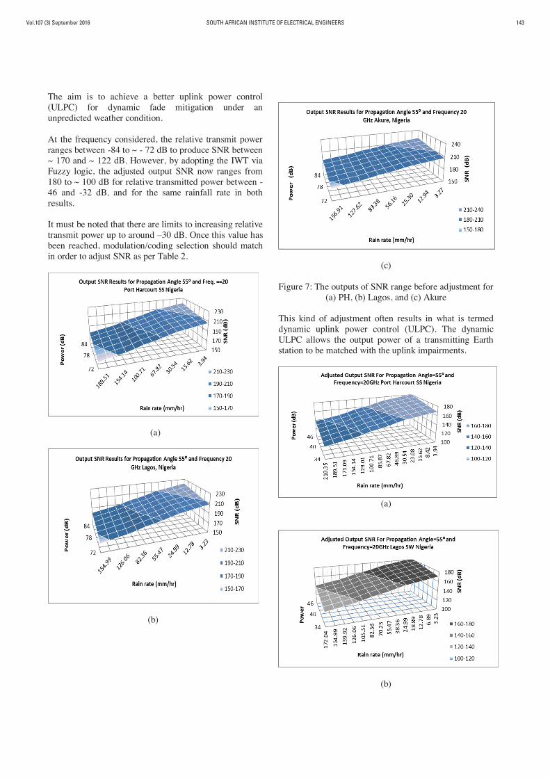
Vol.107 (3) September 2016 SOUTH AFRICAN INSTITUTE OF ELECTRICAL ENGINEERS 143
The aim is to achieve a better uplink power control (ULPC) for dynamic fade mitigation under an unpredicted weather condition. At the frequency considered, the relative transmit power ranges between -84 to ~ - 72 dB to produce SNR between ~ 170 and ~ 122 dB. However, by adopting the IWT via Fuzzy logic, the adjusted output SNR now ranges from 180 to ~ 100 dB for relative transmitted power between -46 and -32 dB, and for the same rainfall rate in both results. It must be noted that there are limits to increasing relative transmit power up to around –30 dB. Once this value has been reached, modulation/coding selection should match in order to adjust SNR as per Table 2.
(a)
(b)
(c)
Figure 7: The outputs of SNR range before adjustment for (a) PH, (b) Lagos, and (c) Akure
This kind of adjustment often results in what is termed dynamic uplink power control (ULPC). The dynamic ULPC allows the output power of a transmitting Earth station to be matched with the uplink impairments.
(a)
(b)

Vol.107 (3) September 2016SOUTH AFRICAN INSTITUTE OF ELECTRICAL ENGINEERS144
(c)
Figure 8: The outputs of SNR range after adjustment for (a) PH, (b) Lagos, and (c) Akure
4. CONCLUSION
This work presents an intelligent technique with the ability to predict channel attenuation due to tropical atmospheric conditions that can enable mitigation of the channel fading condition by adaptively selecting appropriate propagation parameters. At SHF and EHF bands, the relative effect of weather attenuation was so great that an efficient and dependable method for estimating RIA was considered essential for designing efficient and intelligent control systems. This paper has presented a solution to this problem. Here, we estimated the RIA for three locations of study based on the model suitable for a subtropical/tropical region and techniques that bring noticeable improvements in the SNR on satellite communication channels enroute to these regions. This was achieved by utilising RIA estimations in the decision support techniques. The ability to better estimate RIA has resulted in a significant opportunity to model communication channels such that we are able to improve SNR by better tuning of parameters like transmit power, modulation, propagation angle, frequency and transmission rate. The ultimate benefit of this work would be in realising tolerance margins for optimal performances of communication signals under severe tropical weather conditions.
5. ACKNOWLEDGEMENTS
The authors wish to acknowledge the Centre of Radio Access Network and Rural Communication (RAN-RC) Niche Area, Mangosuthu University of Technology (MUT), Umlazi, KZN, South Africa. They are also grateful to Obiyemi O.O. for the data used in the validation in this work.
6. REFERENCES [1] F. Moupfouma: “Improvement of rain attenuation
prediction method for terrestrial microwave links”,
Institute of Electrical Electronics Engineers Transaction on Antennas Propagation, Vol. 32 No. 12, pp. 1368-1372, 1984.
[2] W.P. Qing, J.E. Allnutt and C. Tsui: “Evaluation of
Diversity and Power Control Techniques for Satellite Communication Systems in Tropical and Equatorial Rain Climates”, Antennas and Propagation, IEEE Transactions, Vol. 56, pp. 3293-3301, October 2008.
[3] J.S. Ojo, M.O. Ajewole and S.K. Sarkar: “Rain Rate
and Rain Attenuation Prediction for Satellite Communication in Ku and Ka Bands over Nigeria”, Progress In Electromagnetic Research B, Vol. 5, pp. 207-233, 2008.
[4] B. Segal: “The influence of Rain-gauge integration
Time on Measured Rainfall-Intensity Distribution Functions”, J. Atmos. Oceanic Technology, Vol. 3, pp. 662-667, 1986.
[5] P.L. Rice and N.R. Holmberg: “Cumulative time
statistics of surface point rainfall rates”, Institute of Electrical Electronics Engineers Transaction on Communications, Vol. 21 No.10, pp. 1131-1136, 1973.
[6] C. Ito and Y. Hosoya: “Worldwide 1-min rain rate
distribution prediction method which uses thunderstorm ratio as regional climatic parameter”, Electronics Letters, Vol. 35 No. 18, pp. 1585-1587, 1999.
[7] F. Moupfouma and L. Martin: “Modelling of the
rainfall rate cumulative distribution for the design of satellite and terrestrial communication systems", International Journal of Satellite Communications, Vol. 13 No. 2, pp. 105-115, 1995.
[8] Owolawi, P. A., 2010: Characteristics of rain at
microwave and millimetric bands for terrestrial and satellite links attenuation in South Africa and surrounding islands. Ph.D. thesis, University of KwaZulu-Natal.
[9] V. Kumar and V. Ramachandran: “Rain Attenuation
Measurement at 11.6GHz in Suva, Fiji”, Electronics Letters, Vol. 40 No. 22, pp. 23-25, 2004.
[10] F. Moupfounma: “Model of Rainfall-rate
Distribution for Radio System Design”, IEEE Proceedings, Vol. 132 Pt. H No. 1, pp. 39-43, February 1985.
[11] J.S. Ojo and T.V. Omotosho: “Comparison of 1-min
rain rate derived from TRMM satellite data and rain gauge data for microwave applications in Nigeria”, Journal of Atmospheric and Solar-Terrestrial Physics, Vol. 102, pp. 17-25, 2013.

Vol.107 (3) September 2016 SOUTH AFRICAN INSTITUTE OF ELECTRICAL ENGINEERS 145
[12] K. Harb, C. Huang, A. Srinivasan and B. Cheng: “Intelligent Weather Aware Scheme for Satellite Systems”, IEEE Communications Society proceeding, pp. 1930-1936, 2008.
[13] J.S. Ojo: “Rain Height Statistics Based on 0∘C
Isotherm Height Using TRMM Precipitation Data for Earth-Space Satellite Links in Nigeria”, ISRN Atmospheric Sciences, Vol. 2014, Article ID 798289, 5 pages, http://dx.doi.org/10.1155/2014/798289.
[14] F. Moupfouma: “More about rainfall rate and their
application in predicting radio system engineering”, IEEE Proc., Vol. 134 Pt. H No. 6, pp. 527-537, 1987.
[15] F. Moupfouma: “Electromagnetic Waves
Attenuation due to Rain: A Prediction Model for Terrestrial or L.O.S SHF and EHF Radio Communication Links”, J Infrared Milli Terahz Waves, Vol. 30, pp. 622-632, 2009.
[16] G.O. Ajayi (ed.): Handbook on Radio propagation
Related to Satellite Communications in Tropical and Subtropical Countries, Trieste, Italy, URSI Standing Committee on Developing Countries, and International Center for Theoretical Physics, 1996.
[17] P. ITU-R: “Specific attenuation model for rain for
use in prediction methods”, Recommendation ITU-R, International Telecommunication Union, Geneva, Switzerland, P.838-3, 2003.
[18] E. Lutz, M. Werner, A. Jahn, Satellite Systems for
Personal and Broadband Communications, pages 47-82. Springer, New York, 2000.
[19] K. Harb, F. Richard Yu, P. Dhakal and A.
Srinivasan: “A decision support scheme to maintain QoS in weather impacted satellite Networks”, AIAA Atmospheric and Space Environmental Conference, 2-5 August 2010, Toronto, Ontario, Copyright 2010 by American Institute of Aeronautics and Astronautics, Inc.
[20] A.Chavan and R.D. Patane: “Performance
Improvement of Intelligent Weather System for Satellite Networks” International Journal of Scientific and Research Publications, Volume, Issue 7, July 2015.
[21] D. Driankov, H. Hellenndoorn and M. Reinfrank
“An Introduction to fuzzy Control”, Springer – Verlang, Berlin, New York, 1993.
[22] J.S. Ojo and P.A. Owolawi: “Intelligent Techniques
to maintain QoS at SHF and EHF Satellite Systems Network in a Subtropical Climate”, ICAST conference proceedings, Covenant University,
Sango Otta, Ogun State, Nigeria, pp. 33-39, 29-31 October 2014.
[23] O.O. Obiyemi, T.J.O. Afullo and T.S. Ibiyemi:
“Evaluation of rain degraded digital satellite television reception in tropical region”, International Journal of Scientific & Engineering Research, Vol. 4 No. 12, pp. 790-799, December 2013.
[24] P. ITU-R: “Acquisition, presentation and analysis of
data in studies of tropospheric propagation”, International Telecommunication Union, Geneva, Switzerland, P. 311-15, 2015.

Vol.107 (3) September 2016SOUTH AFRICAN INSTITUTE OF ELECTRICAL ENGINEERS146
NON-CONVEX OPTIMISATION OF COMBINED ENVIRONMENTALECONOMIC DISPATCH THROUGH CULTURAL ALGORITHM WITHTHE CONSIDERATION OF THE PHYSICAL CONSTRAINTS OF GEN-ERATING UNITS AND PRICE PENALTY FACTORS
Arman Goudarzi∗, Afshin Ahmadi†, Andrew G Swanson∗ and John Van Coller‡
∗ School of Engineering, University of KwaZulu-Natal, Durban, 4041, South Africa E-mail: [email protected],[email protected]† Department of Electrical Engineering, Clemson University, Clemson, SC 29634, USA E-mail: [email protected]‡ School of Electrical and Information Engineering, University of the Witwatersrand, Johannesburg,2000, South Africa E-mail:[email protected]
Abstract: Four versions of cultural algorithm have been proposed to find an optimal solution of thecombined environmental economic dispatch problem. The main objective of combined environmentaleconomic dispatch is to simultaneously minimise two competitive objectives of fuel cost and emission,while satisfying various power system constraints such as the valve-point effect, emission costs, theprohibited operation zone, the ramp-rate limit, and the transmission losses. In order to solve thisnon-convex and non-continuous multi-objective optimisation problem with the cultural algorithm, theobjective function has been converted to a single objective function using a technique called pricepenalty factor. Four different types of penalty factors have been examined in this paper. Three differenttest case systems with 5, 20, and 50 generating units have been implemented to investigate the perfor-mance and effectiveness of proposed algorithms. The cultural algorithm shows a superior performancein handling the combined environmental economic dispatch problem in comparison to other methods.
Key words: Combined environmental economic dispatch, cultural algorithm, price penalty factors,prohibited operating zones, ramp-rate limits, valve-point effect
NOMENCLATURE
Index
CA Cultural algorithmCEED Combined environmental economic
dispatchCF Cost functionPF Penalisation factorPPFs Price penalty factorsPOZ Prohibited operating zone
Variables
ai,bi,ci Fuel cost coefficients of unit iαi,βi,γi,ηi,δi Emission cost coefficients of unit idi,ei Fuel cost coefficients of unit i regarding
valve-point effectsBi j i jth element of the loss coefficient
square matrixB0i ith element of the loss coefficient
vectorB00 Loss coefficient constantB(t) Belief space at cultural algorithmFct(P) Total CEED generation costfemc(P) Emission cost functionfgc(P) Generation cost function
hi Coefficient of price penalty factorhmax−max
i Max-Max price penalty factorhmax−min
i Max-Min price penalty factorhmin−max
i Min-Max price penalty factorhmin−min
i Min-Min price penalty factorI j(t) Closed interval at N(t)l,u The lower and upper bound which are
initialised by the domain valuesL j(t) Score of the lower bound at N(t)NG Number of generating unitsN(t) Normative knowledge component of
the cultural algorithmNi j A normalised number for individual i
and component jns Number of variables of situational
componentnx Number of variables of normative
componentnzi Number of prohibited zones for unit iΩ Sets of units having POZPi Power output of unit iPD Load demandPL Power transmission lossP0
i Previous output powerPu
i,nziUpper bound of unit i at prohibitedzone i

Vol.107 (3) September 2016 SOUTH AFRICAN INSTITUTE OF ELECTRICAL ENGINEERS 147
Pmini ,Pmax
i Minimum and maximum generationlimits of the ith generating unit
Pli,l ,P
Ui,l Lower and upper bound of the lth
prohibited zones of unit iPl
i,k,PUi,k Lower and upper bound of the kth
prohibited zones of unit iPl
i,nzi,PU
i,nziLower and upper bound of the nzthprohibited zones of unit i
S(t) Situational knowledge component ofthe cultural algorithm
Si Spinning reserve from unit iSR Total system spinning reserve require-
mentSmax
i Maximum spinning reserve contribu-tion of unit i
δ j Step size of belief intervalδ2
j(t) The variance of normalised number Ni jUj(t) Score of the upper bound at N(t)URi,DRi Up and down ramp rate limits of unit iXj(t) Dimension of belief space at compo-
nent jXl(t) An accepted responsexi j(t) The mean of normalised number Ni jxl j(t) An accepted response of the compo-
nent jxi j(t) Influence functionxmin
j (t),xmaxj (t) Minimum and maximum boundary of
the closed interval at generation ty(t) Best individual of the solution vector
1. INTRODUCTION
Economic dispatch (ED) is an optimisation task in thepower system that attempts to determine the optimaldistribution of power demand among the committedgenerating units for the purpose of minimising totaloperating cost while satisfying a set of equality and in-equality system constraints. With increased environmentalconcerns and given that thermal power plants release asignificant amount of pollutants such as sulphur oxides(SOx), nitrogen oxides (NOx), carbon monoxide (CO), andcarbon dioxide (CO2) into the atmosphere, it has becomeessential to not only minimise the fuel cost but also theemission level of these harmful gases. In [1], severalscenarios of emission reduction such as the installationof pollution control devices, burning low-emission fuels,replacement of aged fuel burners and the use of renewableenergy resources have been considered for a combinedenvironmental economic dispatch (CEED) problem. Thelatter solution has become an attractive short term strategydue to its economic advantages and ease of implementation[2, 3]. CEED is a multi-objective optimisation problemthat attempts to simultaneously minimise two competitiveobjectives of fuel cost and emission of gaseous pollutantswhich are both related to system constraints.
Various techniques have been proposed for the CEEDproblem. The majority of the algorithms can becategorised as either mathematical or evolutionaryoptimisation techniques. Mathematical techniques have
fast computational time and are able to find near exactsolutions for convex problems through a convex objectivefunction and their respective domains, while sometimesthey would fall into local minima or maxima. Someresearchers have tried to develop mathematical methods tohandle the CEED problem. Nanda et al. aimed to solve theCEED problem concerning the line power flow constraintby developing a classical technique based on coordinationequations [4]. A single objective function using a linearcombination of different objectives as a weighted sum wasdeveloped in [5]. Unfortunately, multiple runs are requiredfor this method and it also fails to solve non-convexfunctions [6]. A nonlinear unconstrained/constrainedmulti-objective mathematical formulation based on a fastε-constraint approach was introduced in [7] where fuelcost and environmental impact were treated as competingobjectives.
The CEED problem becomes a nonlinear, non-convex andnon-continuous optimisation problem when the real-worldpower system constraints such as valve point effect,prohibited zone, ramp rate limits, and transmission lossesare considered [8–10]. It is impractical to find aunique optimal solution using mathematical techniqueswith respect to all these constraints. To tackle this issue,researchers have applied heuristic optimisation algorithmsto solve the CEED problem. These methods usuallydeal with non-smooth non-convex functions but, as adrawback, the computational time is long since they carryout a population of potential solutions simultaneously.Applications of different heuristic techniques pertaining tothe CEED problem have been reported in literature. In[8], the price penalty approach has been presented, wherethe bi-objective CEED problem was converted to a singleobjective through to the max-max price penalty factor,after which various heuristic techniques such as geneticalgorithm (GA), evolutionary programming (EP), particleswarm optimisation (PSO), and differential evolution (DE)were applied to obtain and compare the solutions for theIEEE 30-bus system and 15-unit system. The valve-pointeffect and transmission losses were not considered in[8]. In [11], the applicability of biogeography-basedoptimisation technique to find the solution of CEEDproblem has been presented. The proposed algorithmwas implemented in three, six and fourteen generator testsystems and results were compared to the solutions basedon Newton-Raphson, Tabu search, GA, non-dominatedsorting genetic algorithm (NSGA), fuzzy logic controlledgenetic algorithm, PSO and DE. A game theory basedmodel was developed in [3] to address the multi-objectivedynamic economic emission dispatch problem taking intoaccount transmission losses. Senthil proposed a lambdabased approach using EP to solve the CEED problemconsidering powering limits [12]. The algorithm wastested on a power system consisting of three and sixgenerators. A gravitational search algorithm has beensuggested for the solution of the CEED problem in [13–16]and various test cases with and without the valve-pointeffect and transmission losses were considered in thesestudies. Many other heuristic algorithms such as NSGA-II

Vol.107 (3) September 2016SOUTH AFRICAN INSTITUTE OF ELECTRICAL ENGINEERS148
[17, 18], bacterial foraging [19–21], enhanced fireflyalgorithm [22], advanced parallelised PSO [23], fuzzifiedmulti-objective PSO [24], multi-objective chaotic PSO[25], opposition-based harmony search algorithm [26], beecolony [2] and several others have been reported in theliterature to obtain a solution to the CEED problem.
Cultural algorithm (CA) is an evolutionary optimisationmethod which was first introduced by Reynolds in 1994[27]. Cultural algorithm consists of an evolutionarypopulation space (genetic component) and a belief space(cultural principals). CA was initially designed to handlesingle objective optimisation problems. To cope withmulti-objective problems, either a hybrid optimisationalgorithm should be developed or the multi-objectivefunction should be converted to a single function. Fewstudies have successfully implemented CA for the solutionto the CEED problem. In [28], evolutionary programmingwas embedded into CA for this purpose and constraintssuch as ramp rate limits, prohibited zone of operation,valve point loading effects and transmission losses wereconsidered. The method was tested on three, sixand fourteen generator systems. Rui Zhang et al. [6]developed a hybrid PSO-CA technique to address theCEED problem when considering prohibited operatingzones and generator limits. Two test systems wereimplemented to verify efficiencies of the proposed method.A hybrid multi-objective cultural algorithm method waspresented in [29] to carry out the optimal short-termenvironmental/economic hydrothermal scheduling. Theproposed hybrid method combined a differential evolution(DE) algorithm into the framework of CA.
In this study, an approach based on the price penaltyfactor, i.e. ratio of fuel cost to emission value, has beenused to convert the multi-objective combined emissionand economic dispatch problem into a single objectivefunction. To replicate a real-world power system,the following constraints of generating units such asramp-rate limits, prohibited operating zones, valve-pointeffect, and transmission losses have been considered.The effectiveness of CA in handling complex CEEDproblems has been verified on three test systems with5, 20 and 50 generating units and non-smooth fuel costfunctions. Simulation results have been compared withother heuristic optimisation techniques such as biographybased optimiser (BBO), restricted ant colony optimiser(ACOR), artificial bee colony (ABC), PSO, GA, hybridGA and PSO (GAPSO), and firefly algorithm (FA). Themain contributions of this paper are as follows: i)four different versions of cultural algorithm have beenemployed to solve CEED problem. To the best of authors’knowledge, a similar study has never been reported; ii)the impact of four different types of penalty factor onthe final price has been examined. No other study hasinvestigated the effect of different penalty factors forthe same power system; iii) the test system with 50generators, when considering all the constraints of thegenerating units, imposes significant non-linearity to thesystem. The convergence to the optimal solution willbecome cumbersome as it is the largest reported test case
for solving the CEED problem.
The organisation of this study is as follows. Section 2demonstrates the problem formulation and mathematicalmethods. Section 3 provides simulation results, wherethe effectiveness and superiority of the proposed methodto solve the CEED problem has been discussed.Subsequently, the conclusion is given in Section 4.
2. PROBLEM FORMULATION
2.1 Combined Environmental Economic Dispatch(CEED)
The main objective of classical economic load dispatch(ELD) is to minimise the total cost of generationby determining the optimum scheduling of generatingunits and ensuring the satisfaction of system constraints.This study has divided the operation constraints intotwo different categories. The first category is relatedto the particular characteristics of the generating unitssuch as generation capacity, the valve-point effect andenvironmental emission levels, while the second one isassociated with physical constraints such as ramp ratelimits, prohibited operating zones and spinning reservelevels.
The cost objective function of CEED can be representedby a quadratic cost function [30]:
fgc(Pi) =NG
∑i=1
(ai +biPi + ciP2i ) [$/h] (1)
The effect of valve-point loading can be modelled byadding a recurring rectified term to the main cost functionas given in [30], where the cost function curve with theeffect of valve-point loading is shown in Fig. 1:
fgc(Pi) =NG
∑i=1
[(ai +biPi + ciP2i )
+|di sin(ei × (Pmini −Pi))|] [$/h] (2)
Figure 1: Fuel cost function curve for CEED withvalve-point loading effect

Vol.107 (3) September 2016 SOUTH AFRICAN INSTITUTE OF ELECTRICAL ENGINEERS 149
Most thermal and fossil-based generating units are majorsources of NOx, and have been strictly advised by theenvironmental protection agency (EPA) to reduce theiremissions. In this study, the emission of NOx is consideredto be optimally moderated from the environmentalpreservation point of view. The emission cost function,including the valve-point effect, can be expressed asfollows [31]:
femc(Pi) =NG
∑i=1
[(αi +βiPi + γiP2i )+ηi exp(δiPi)] [lb/h]
(3)
The total generation cost of CEED as a multi-objectiveoptimisation can be converted into a single objectivefunction through the combination of generation cost andemission cost as well as the consideration of the pricepenalty factor hi [32]:
Fct(Pi) = fgc +hi × femc(Pi) (4)
Fct(Pi) =NG
∑i=1
[(ai +biPi + ciP2i )+ |di sin(ei × (Pmin
i −Pi))|]
+hi ×NG
∑i=1
[(αi +βiPi + γiP2i )+ηi exp(δiPi)] [$/h]
(5)
The proposed CEED objective function is subject to thefollowing constraints:
Equality constraint: The total power output of the systemshould be capable of meeting the total load demand andpower losses (I), and in the case of a lossless systems itshould be able to satisfy the total load demand (II).
(I)NG
∑i=1
Pi = PD +PL (6)
(II)NG
∑i=1
Pi = PD (7)
The power loss of the system can be determined by Korn’sloss formula [33]:
PL =N
∑i=1
N
∑j=1
PiBi jPj +N
∑i=1
B0iPi +B00 (8)
Or re-written in matrix notation as:
PL = PT [B]P+B0P+B00 (9)
Inequality constraint: For stable operation, all generatingunits are strictly constrained to operate at their minimumand maximum generation limits; consequently the
inequality constraint is:
Pmini ≤ Pi ≤ Pmax
i for i = 1,2,3 . . .NG (10)
Ramp rate limit: conforming to [34], the inequalityconstraints due to ramp rate constraints for changes ingeneration levels are modified; (I) as generation increasesand (II) as generation decreases.
(I) Pi −P0i ≤URi (11)
(II) P0i −Pi ≤ DRi (12)
By considering the inequality constraints, equations (11)and (12) can be rewritten:
max(Pmini ,P0
i −DRi)≤ Pi ≤ min(Pmaxi ,P0
i +URi) (13)
Fig. 2 shows the mechanism of the generating units whenconsidering the ramp rate limits.
Figure 2: Operation of generating units when consideringthe ramp rate limits
Prohibited operating zone (POZ): the POZ is an intervalin which generating units are not able to operate due to theinherent nature of thermal units that may have steam valveoperation or vibrations in the shaft bearings. The principleof POZ has been depicted in Fig. 3. The feasible operatingzones of unit i are described as [35]:
Pmini ≤ Pi ≤ Pl
i,lPu
i,l ≤ Pi ≤ Pli,k
Pui,k ≤ Pi ≤ Pl
i,nziPu
i,nzi≤ Pi ≤ Pmax
i
for k = 1,2,3 . . .nzi ∀i /∈ Ω
(14)
Spinning reserve: to have a reliable operation a minimumspinning reserve should be considered to meet the loadfluctuation and unforeseen outages of the generating units

Vol.107 (3) September 2016SOUTH AFRICAN INSTITUTE OF ELECTRICAL ENGINEERS150
and grid components [35]:
NG
∑i=1
Si ≥ SR (15)
Where:
Si = min(Pmaxi −Pi,Smax
i ); Si = 0;∀i ∈ Ω (16)
Where Ω is related to sets of units having POZs. It issignificant to mention that spinning reserve will be carriedout from units without POZs. Those units having noPOZs are responsible for maintaining the system spinningreserve requirements which can be set as a fraction of theload demand or equal to the capacity of the largest unit[36].
Figure 3: Fuel cost function curve with prohibited operatingzones
Price penalty factors: Four different types of pricepenalty factors (PPFs) are proposed. PPFs describe theproportion between fuel cost and emission cost curveswithout considering the valve point effect. The PPFs areas follows:
Max-Max:
hmax−maxi =
ai +biPmaxi + ci(Pmax
i )2
αi +βiPmaxi + γi(Pmax
i )2 [$/lb] (17)
Max-Min:
hmax−mini =
ai +biPmaxi + ci(Pmax
i )2
αi +βiPmini + γi(Pmin
i )2 [$/lb] (18)
Min-Max:
hmin−maxi =
ai +biPmini + ci(Pmin
i )2
αi +βiPmaxi + γi(Pmax
i )2 [$/lb] (19)
Max-Max:
hmin−mini =
ai +biPmini + ci(Pmin
i )2
αi +βiPmini + γi(Pmin
i )2 [$/lb] (20)
The main purpose of PPFs is to convert the physicalimplication of the emission standard from the emissionweight to the fuel cost of the emission.
2.2 Evaluation of generation levels
To ensure that the equality constraint of the system isalways maintained, this study proposes a power balanceviolation (PBV) formulation to continuously satisfy theequality constraint. Equation (6) is rewritten as:
NG
∑i=1
Pi ≥ PD +PL (21)
by modification of equation (21), the PBV is formulatedas:
PBV = max
(1− ∑NG
i=1 Pi −PL
PD,0
)(22)
As long as equation (21) is satisfied then the PBV is equalto zero. To maintain the equality constraint and find themost optimal solutions in the search space, the algorithmaccepts the solutions which are able to hold the followingrelation:
PD +PL −NG
∑i=1
Pi = 0 (23)
To accelerate the process of convergence to achieveoptimal solutions, this study has used an evaluationfunction to push the answers of the optimisation algorithmtowards the most optimum solution possible by means ofa penalisation factor. The proposed method evaluationfunction which would be evaluated for each iteration isformulated as:
Feval = Fct(Pi)× (1+PF ×PBV ) (24)
In this study PF has been considered to be equal to 1000,in many practical problems, the selection of the parametersis subject to the characteristics of the problem.
2.3 Cultural Algorithms
The principles behind the cultural algorithm were proposedby Reynolds in 1994 [27]. CA is a type of computationalintelligence algorithm which is inspired by the culturalinheritance process of several generations. The idea of thisinnovative optimisation technique is that culture has thepotential to be emblematically encoded and shared amongpopulations of a society [37].

Vol.107 (3) September 2016 SOUTH AFRICAN INSTITUTE OF ELECTRICAL ENGINEERS 151
The mechanism of CA is based on the discovery of anelite individual in a population, and setting the aim of thepopulation to reach the same level as the elite’s knowledge.The culture evolution of the population would improve theadaptability of the individuals towards the targeted aimsand the speed of this process would be increased throughguidance by the elite’s knowledge.
The basic concepts of cultural algorithm: Culture is theaccumulated experience and learned behaviour of a groupof people which can be called the tradition of that group ofpeople and which is maintained through generations.
CA is composed of two basic spaces: population space(to illustrate a genetic component according to DarwinianTheory) and belief space (to illustrate cultural principles)which differentiate the CAs from other evolutionaryalgorithms [37]. The population space represents andcategorises the individuals based on their specificationsin each set, while the belief space collects the knowledgeobtained by individuals.
At each iteration of CA, individuals in their populationspace can be substituted and updated by some of theirgenerations via a communication protocol. This processcan be handled by implementing any population-basedoperators or any other evolutionary algorithms such asABC, BBO, or FA [6]. The framework of CA is depictedin Fig. 4.
Figure 4: Illustration of conceptual framework of culturalalgorithm based on the two spaces
In each generation, individuals would be evaluated bythe fitness function that is determined by the evolutionaryalgorithm in the population space. Thereafter, anacceptance function is utilised to specify which individualsin the current population have a major influence on currentbeliefs.
The experience that has been acquired by acceptedindividuals would be applied to adjust the beliefs. Once
the beliefs have been adjusted then they will be used toinfluence the improvement of the population. In orderto vary the population space, the variation operators areresponsible for using the beliefs to regulate the changesin individuals, where it is possible to use a crossover andmutation function or a self-adapting control parameter asthe variation operator [38].
Belief space: comprises a set of experience and knowledgestructure of the individuals. Based on Engelbrecht [38],CA is composed of four sections, such as: knowledgecomponents, acceptance functions, belief space adjustmentand influence functions.
The sections of belief space are introduced as follows:
(1) Knowledge component: The belief space stores aset of knowledge components in order to demonstratethe behavioural patterns of accepted individuals from thepopulation space. The forms of knowledge componentsand representation of data structure depends on thecharacteristics of the problem. This study has used thevector representations to describe this component [39].The belief space can be categorised in two knowledgecomponents [39]:
(1.1) situational knowledge component: this componentis responsible for finding the best solution in a particularperiod of time or a generation.
(1.2) normative knowledge component: this componentprovides a criterion for each individual behaviour whichwould be considered as a guideline for the mutationaladjustment of individuals. In the process of optimisationthese norms or intervals specify the suitable range that canbe searched in each dimension.
The belief space can be mathematically expressed basedon the definition of its components [38-39]:
B(t) = (S(t),N(t)) (25)
Where:
S(t) = y1(t) : l = 1,2,3, . . . ,ns (26)
N(t) = (X1(t),X2(t),X3(t), . . . ,Xnx(t)) (27)
For each dimension of belief space the followinginformation is required to be saved:
Xj(t) = (I j(t),L j(t),Uj(t)) (28)
Subject to:
I j(t) = [xminj ,xmax
j ] = [l,u] (29)
(2) Acceptance functions: To shape the beliefs ina particular population, this function decides whichindividuals of population will be utilised for this purpose.

Vol.107 (3) September 2016SOUTH AFRICAN INSTITUTE OF ELECTRICAL ENGINEERS152
Acceptance functions can be arithmetically designed intwo ways [38]:
(2.1) static: n% individuals of a population will beselected.
(2.2) dynamic: by using any selection methods ofevolutionary algorithms such as elitism or roulette-wheelselection.
In this study, the number of the selected individuals isdetermined by the following method according to [38]:
nB(t) =[ntotγ
t
],γ ∈ [0,1] (30)
Where:
nB is the number of selected individualsfor forming the beliefs in a population
t is the number of iterations (generation)npop is the number of population
(3) Belief space adjustment: after selecting the numberof individuals to form the beliefs, the interval ofknowledge components can be updated through thefollowing formulation [38-39]:
(3.1) Situational knowledge:
S(t +1) = y(t +1) (31)
Where:
y(t +1) =
minl=1,...,nB(t) Xl(t) i f f (minl=1,...,nB(t) Xl(t))< f (y(t)
y(t) otherwise(32)
(3.2) Normative knowledge:
xminj (t +1) =
xl j(t) i f xl j(t)≤ xminj (t)
or f (Xl(t))< L j(t)xmin
j (t) otherwise(33)
For updating L j(t):
L j(t +1) =
f (X)l(t)) i f xl j(t)≤ xminj (t)
or f (Xl(t))< L j(t)L j(t) otherwise
(34)
xmaxj (t +1) =
xl j(t) i f xl j(t)≤ xmaxj (t)
or f (Xl(t))<Uj(t)xmax
j (t) otherwise(35)
For updating Uj(t):
Uj(t +1) =
f (X)l(t)) i f xl j(t)≤ xminj (t)
or f (Xl(t))<Uj(t)Uj(t) otherwise
(36)
Where:
Xl(t), l = 1,2,3 . . . ,nB(t) (37)
(4) Influence functions: the responsibility of thesefunctions is to influence the population space based onthe adjusted beliefs in order to define the mutational stepsize, and the direction of change. All the CAs havethe same procedure until this point, the study proposesdifferent versions of CAs according to their influencefunction specifications. As mentioned in [38-39], the CAsare categorised in four different versions:
(4.1) Cultural algorithm version 1 (CA1): only thenormative knowledge component is used to specify stepsizes.
xi j(t) = xi j(t)+δ j ×Ni j(0,1) (38)
Equation (37) can be rewritten as:
xi j(t) = xi j(t)+δ j ×Ni j(0,1) (39)
Where:
δ j(t) = [xmaxj (t)+ xmin
j (t)] (40)
(4.2) Cultural algorithm version 2 (CA2): only thesituational knowledge component is used to specify thedirection changes. In this version of CA, we assume thestrategy parameter is greater than zero (σi j > 0).
xi j(t) =
xi j(t)+ |σi jNi j(0,1)| i f xi j(t)< y j(t)xi j(t)−|σi jNi j(0,1)| i f xi j(t)> y j(t)xi j(t)+σi jNi j(0,1) otherwise
(41)
(4.3) Cultural algorithm version 3 (CA3): this versionis the combination of both knowledge components. Thesituational knowledge component is used to specify thestep sizes, while the normative knowledge component isused for direction changes. The definition of xi j(t) willremain the same as CA2, but the strategy parameter wouldbe redefined as:
σi j(t) = α[xmaxj (t)+ xmin
j (t)],0 < α < 1 (42)
Where α denotes the ratio of the strategy parameter.
(4.4) Cultural algorithm version 4 (CA4): in the fourthversion of CA, the normative knowledge component isassigned to handle the step sizes and direction changes.
xi j(t) =
xi j(t)+ |σi jNi j(0,1)| i f xi j(t)< xminj (t)
xi j(t)−|σi jNi j(0,1)| i f xi j(t)> xmaxj (t)
xi j(t)+βσi jNi j(0,1) otherwise(43)
In CA4, the scaling factor is applicable for all positivevalues (β > 0), and the strategy parameter can be definedas is described in CA3. In all versions of CA influence

Vol.107 (3) September 2016 SOUTH AFRICAN INSTITUTE OF ELECTRICAL ENGINEERS 153
functions, subscript i denotes the individual and subscriptj describes the type of the knowledge component.
3. RESULTS AND DISCUSSION
The proposed algorithms were tested on different scenariosof CEED that consider several physical constraints ofgenerating units and system, including:
• with and without transmission loss• with and without maintaining spinning reserve
constraint• with and without prohibited operating zones• valve-point effect• ramp rate limits• fuel emission constraint• price penalty factors
To investigate and verify the robustness of the proposedmethods, they were tested on three different systems of5, 20 and 50 generating units respectively. All methodswere implemented and compared in this study to show thecapability of the methodology. The codes and algorithmswere developed on MATLAB 2013a to perform the casestudies and executed on a personal computer with thefollowing specifications, Intel CoreT M i7-3770 (3.40GHz), 8.00 GB RAM (DDR5) and windows 8.1 operatingsystem.
As all the evolutionary algorithms are highly sensitiveto the tuning of their decision parameters and variables,the study selected the suitable settings for all versions ofCA. These parameters are population size npop, acceptanceratio Paccept , ratio of strategy parameter α, scalingcoefficient β set to 50, 0.15, 0.25, and 0.5 respectively.To have a uniform comparison among all comparedevolutionary algorithms, the spinning reserve requirementwas set to 5% of total load demand as in [1]. The maximumiterations for all the trials were fixed to 300.
To validate the effectiveness of the proposed method of thestudy, the following case studies have been analysed andcompared:
Case 1: 5 generating units; without considering POZ
Case 2: 20 generating units (four times replication ofthe test system of case 1); without considering powertransmission losses and maintaining spinning reserve
Case 3: 50 generating units (ten times replication ofthe test system of case 1); without considering powertransmission losses and maintaining spinning reserve
3.1 Case 1
A small test system comprising of 5 generating units wasconsidered based on [40–42] with a minor modificationof the test system. The system specifications are given inTable (1), (2) and (3). The loss coefficients (B-coefficients)of the transmission network are given in Table (4), wherethe values are expressed in p.u. on a 100 MVA base. Table1 lists the physical operating limits and cost coefficientsof generating units such as quadratic cost, proportionalcost and fixed cost. Table 2 lists the ramping limitsas well as the quantitative information of the prohibitedzones for the generating units. Table 3 lists a detailedassociated emission cost for the NOx through its respectivecoefficients costs. The valve-point effect, ramp rate limits,spinning reserve requirement, emission constraints andthe effect of price penalty factors (PPFs) on the totalgeneration cost were considered for the study. The totalload demand of the test system was 730 MW. In thiscase, 100 trials have been carried out for the purpose ofproducing the results.
The convergence processes of the proposed algorithm withdifferent PPFs are shown in Fig 6 (a, b, c and d) where thetotal cost is plotted against the number of iterations. Theobtained results are compared with BBO, ACOR, ABC,PSO, GA, the combination of GA and PSO (GAPSO), FA.Fig. 6.a shows the convergence process with Max-MaxPPF. As shown, CA3 has the second highest initial guess,however it reaches its optimum level in less than 50iterations with the last step of reduction occurring atthe 50th iteration with a best minimum cost of 2039.46($/h). In terms of the convergence process, most of thealgorithms have reached their optimum level after the 50thiteration, with BBO only succeeding in reach to the finaliteration at close to the 250th iteration.
By analysing Fig. 6(a, b, c and d), it can be seen that theproposed method is the most capable technique to find thebest solution where its best obtained cost is at Min-MaxPPF at 2039.17 ($/h). It is noticeable for all PPFs cases, theproposed method has achieved the final optimisation stagein less than 70 iterations, which indicates the convergencespeed of the proposed method. The maximum cost,average cost, minimum cost and average elapsed timefor the proposed method and other methods are shownin Table (5). For ease of comparison, the elapsed timeof each method is evaluated as an average. From Table(5), it is evident that the proposed method has achievedthe lowest average time and minimum total generationcost with respect to all PPFs cases among all the othermethods. The most optimum average cost was achievedby CA3 through Min-Max PPF at 2042.5414 ($/h), wherethe average elapsed time was 2.4571 seconds.
The breakdown of generator schedules is given in Table(6). The best solution in the solution space is shown inFigure (5), where the best solution is the solution thathas the lowest total cost and lowest emission cost withoutviolating any physical constraint.

Vol.107 (3) September 2016SOUTH AFRICAN INSTITUTE OF ELECTRICAL ENGINEERS154
Figure 5: Best obtained solution in the solution space for case 1
Table 1: Cost coefficients and physical operating limits of generating units
Unit ai ($/h) bi ($/MWh) ci $/(MW )2h di ($/h) ei (1/MW ) Pmini (MW ) Pmax
i (MW )
1 25 2 0.008 100 0.042 10 752 60 1.8 0.003 140 0.04 20 1253 100 2.1 0.0012 160 0.038 30 1754 120 2 0.001 180 0.037 40 2505 40 1.8 0.0015 200 0.035 50 300
Table 2: Ramp rate limits and POZ information of generating units
Unit P0i (MW ) URi (MW ) DRi (MW ) POZi (MW )
1 70 30 30 [60 65]2 100 30 30 [70 75]3 150 40 40 [120 125]4 110 50 50 [80 90]5 270 50 50 [230 240]
Table 3: Emission curve coefficients of generating units
Unit αi (lb/h) βi (lb/MWh) γi lb/(MWh)2h ηi (lb/h) δi (1/MW )
1 80 -0.805 0.018 0.655 0.028462 50 -0.555 0.015 0.5773 0.024463 60 -1.355 0.0105 0.4968 0.02274 45 -0.6 0.008 0.486 0.019485 30 -0.555 0.012 0.5053 0.02075
Table 4: The transmission loss coefficients
0.000049 0.000014 0.000015 0.000015 0.0000200.000014 0.000045 0.000016 0.00002 0.000018
B 0.000015 0.000016 0.000039 0.000010 0.0000120.000015 0.000020 0.000010 0.000040 0.0000140.000020 0.000018 0.000012 0.000014 0.000035

Vol.107 (3) September 2016 SOUTH AFRICAN INSTITUTE OF ELECTRICAL ENGINEERS 155
(a) Max-Max PPF
(b) Max-Min PPF
(c) Min-Max PPF
(d) Min-Min PPF
Figure 6: Convergence process of CEED cost (5 generating units)

Vol.107 (3) September 2016SOUTH AFRICAN INSTITUTE OF ELECTRICAL ENGINEERS156
Table 5: Comparison of the obtained results for case 1
5 Units System Max Cost Avg Cost Min Cost Avg Elapsed Time (s)Max Max 2054.5656 2047.5029 2045.8321
BBO Max Min 2065.2573 2061.2359 2059.9912 8.4732Min Max 2050.3511 2046.0231 2044.6514Min Min 2052.2072 2049.5228 2046.7632Max Max 2305.1833 2067.3245 2041.4102
ACOR Max Min 2167.204 2057.1314 2054.7065 6.2199Min Max 2187.797 2049.3181 2039.7443Min Min 2144.6517 2049.8958 2044.4932Max Max 2047.8929 2046.2479 2046.5098
FA Max Min 2062.8454 2061.1854 2061.6578 2.8594Min Max 2047.8448 2045.8421 2046.1733Min Min 2051.3145 2049.3753 2049.9321Max Max 2049.5923 2047.374 2046.5013
GAPSO Max Min 2063.0634 2062.4204 2061.5215 23.2906Min Max 2049.798 2047.1124 2046.2341Min Min 2051.9561 2050.6466 2049.9444Max Max 2049.7785 2047.5568 2046.5321
PSO Max Min 2063.3545 2062.5546 2061.7235 4.2648Min Max 2049.8845 2047.3345 2047.3121Min Min 2051.9623 2050.7465 2050.2632Max Max 2049.8701 2048.0021 2046.6845
GA Max Min 2063.4025 2062.6801 2061.9432 5.4049Min Max 2050.1478 2047.7468 2046.3145Min Min 2051.8845 2050.8865 2050.2842Max Max 2049.9904 2049.9879 2047.3458
ABC Max Min 2064.6541 2062.8788 2063.23 6.3695Min Max 2050.7456 2048.4563 2048.2032Min Min 2052.3545 2051.0002 2051.4433Max Max 2061.4022 2053.9172 2051.1125
CA1 Max Min 2081.2015 2068.8055 2066.1124 1.2386Min Max 2061.2573 2053.1706 2052.0645Min Min 2065.9603 2056.1002 2053.1237Max Max 2061.8546 2053.9832 2049.3154
CA2 Max Min 2081.5487 2069.0458 2065.9541 1.2594Min Max 2061.7568 2054.0001 2051.0123Min Min 2066.1254 2056.7453 2051.7311Max Max 2053.7469 2042.1457 2039.4621
CA3 Max Min 2063.6157 2056.2873 2053.9714 1.3578Min Max 2055.5814 2042.5414 2039.1724Min Min 2056.2588 2045.6611 2042.8214Max Max 2053.8546 2042.5436 2040.9012
CA4 Max Min 2063.7654 2057.021 2054.4532 1.3281Min Max 2056.3254 2042.8547 2039.6714Min Min 2056.5487 2045.8745 2043.3302

Vol.107 (3) September 2016 SOUTH AFRICAN INSTITUTE OF ELECTRICAL ENGINEERS 157
Table 6: The best obtained solutions of the proposed method (CA3) for case 1
No. of units 1 2 3 4 5Schedule (MW) 32.2494 108.7979 161.0268 226.8128 212.3711
Generation Cost ($/h) 97.8191 291.3472 469.2718 625.0697 489.9202Valve-point Cost ($/h) 1.6309 8.6734 13.8865 21.6623 19.8049Emission Cost ($/h) 0.0076 0.0218 0.0119 0.026 0.0247
Total Cost ($/h) 2039.178Ploss (MW) 11.258
3.2 Case 2
In order to demonstrate the robustness of the proposedmethod on a larger test system, the proposed method wasapplied to a 20 unit system. All the physical constraintsof generating units as described in case 1 (aside fromthe spinning reserve requirement) as well as the effect ofPOZs were considered in this case. The total load demandwas 2920 MW. In this case, transmission line losses wereneglected. To have the refinement process 100 runs havebeen performed for each method. The comparison betweenthe proposed method and the other evolutionary algorithmsduring the convergence process with the consideration oftheir PPFs are depicted in Fig 8 (a, b, c and d).
It is clear from Fig 8 (a, b, c and d) that the proposedmethod provides the lowest cost among the other methodsin all cases. The convergence process has been extendedin all methods due to the enlargement of the test system;nevertheless the proposed method has converged in lessthan 100 iterations which indicates its effectiveness. It isnoticeable that the Min-Max and Min-Min PPFs providethe lowest and highest total generation cost for the
proposed method with costs of 8057.23 and 8070.21($/h) respectively. The detailed results of 20 unit systemwith respect to all PPFs are shown in Table (7). Itis clear that the proposed method obtained the lowestgeneration cost when compared to other techniques, wherethe minimum average cost was computed by its Min-MaxPPF to be 8062.7931 ($/h). It is significant to mentionthat even by enlarging the test system where the degreesof non-convexity and non-linearity of the problem weresignificantly increased, the proposed method managed tomaintain a fast run time and its efficiency where thedifference by the previous case is only 1.0993 s. Theproposed method in comparison to the other versions ofcultural algorithm has a slightly longer time to convergeas it is using both knowledge components (situational andnormative) for its influence function. Figure (7) illustratesthe best obtained solution in the solution space where thebest solution is the solution that has the lowest total costand lowest emission cost without violating any physicalconstraint. Table (8) lists the best solution detailedinformation for generator schedules and their associatedcosts.
Figure 7: Best obtained solution in the solution space for case 2
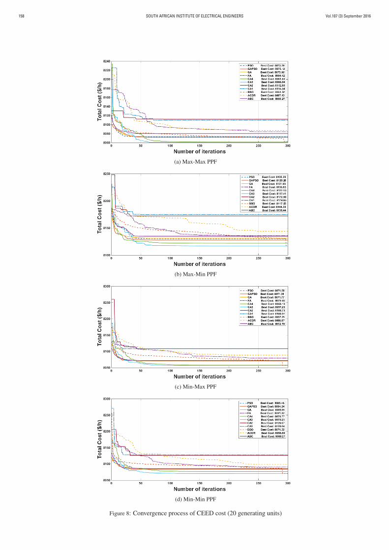
Vol.107 (3) September 2016SOUTH AFRICAN INSTITUTE OF ELECTRICAL ENGINEERS158
(a) Max-Max PPF
(b) Max-Min PPF
(c) Min-Max PPF
(d) Min-Min PPF
Figure 8: Convergence process of CEED cost (20 generating units)

Vol.107 (3) September 2016 SOUTH AFRICAN INSTITUTE OF ELECTRICAL ENGINEERS 159
Table 7: Comparison of the obtained results for case 2
20 Units System Max Cost Avg Cost Min Cost Avg Elapsed Time (s)Max Max 8098.153 8074.88 8063.5204
BBO Max Min 8144.5893 8132.983 8117.5522 24.3705Min Max 8090.8475 8073.56 8057.7132Min Min 8103.9127 8089.66 8071.3245Max Max 8111.0125 8095.4521 8087.1253
ACOR Max Min 8201.5435 8185.4565 8144.3356 15.2124Min Max 8225.5423 8100.0204 8088.6745Min Min 8254.8457 8116.1024 8098.6974Max Max 8104.181 8083.8803 8084.4253
FA Max Min 8171.9771 8142.0902 8135.8323 2.8965Min Max 8100.926 8082.7155 8079.5345Min Min 8129.6365 8098.029 8091.0254Max Max 8083.9209 8073.9642 8072.1245
GAPSO Max Min 8141.7844 8131.5726 8128.2845 29.0153Min Max 8083.1013 8072.2043 8071.3847Min Min 8093.1127 8085.701 8084.2456Max Max 8101.2544 8088.4521 8073.5412
PSO Max Min 8145.5478 8134.8542 8130.2045 8.4742Min Max 8090.6545 8086.7546 8071.5942Min Min 8125.6587 8097.5687 8085.4675Max Max 8107.8542 8089.4574 8073.9245
GA Max Min 8187.5687 8135.8765 8131.8345 9.5049Min Max 8100.2548 8088.5544 8071.7745Min Min 8145.6578 8101.2587 8085.9175Max Max 8212.45 8100.4525 8080.2745
ABC Max Min 8275.3587 8175.6547 8135.4457 13.4197Min Max 8212.5435 8111.5478 8072.7065Min Min 8346.5435 8101.4587 8086.2745Max Max 8188.5478 8135.4578 8114.0423
CA1 Max Min 8254.5478 8178.7723 8174.8545 2.1535Min Max 8145.8528 8122.7744 8108.9147Min Min 8185.9874 8150.5547 8128.6475Max Max 8133.5874 8117.5153 8112.5954
CA2 Max Min 8194.3054 8175.8547 8172.5874 2.3326Min Max 8134.3103 8109.3466 8108.7387Min Min 8150.7771 8128.0509 8126.6787Max Max 8104.6353 8067.5709 8060.8475
CA3 Max Min 8158.7169 8118.3626 8117.4178 2.4571Min Max 8102.5586 8062.7931 8057.2354Min Min 8113.2448 8074.6219 8070.2145Max Max 8104.7854 8079.8745 8061.6354
CA4 Max Min 8167.5841 8137.8745 8122.7854 2.4003Min Max 8103.0124 8078.4658 8058.1088Min Min 8113.4521 8095.5478 8076.7754

Vol.107 (3) September 2016SOUTH AFRICAN INSTITUTE OF ELECTRICAL ENGINEERS160
Table 8: The best obtained solutions of the proposed method (CA3) for case 2
No. of units Schedule (MW) Generation Cost ($/h) Valve-point Cost ($/h) Emission Cost ($/h)1 56.2537 162.8232 3.3899 0.00972 108.0018 289.3965 8.5958 0.02153 167.0662 484.3324 14.5249 0.01334 192.4141 541.8513 17.6879 0.01775 240 558.4 23.1608 0.03276 34.8082 104.3093 1.8184 0.00777 104.7494 281.4661 8.2784 0.02048 140.8305 419.544 11.7503 0.0089 228.4784 629.1591 21.8545 0.026310 240.6657 560.0783 23.2416 0.03311 43.9795 128.4326 2.4906 0.008312 104.1066 279.9063 8.2157 0.020213 151.0329 444.5421 12.8297 0.009814 183.0794 519.6769 16.6077 0.015815 252.4492 590.0045 24.6708 0.037116 32.08 97.3929 1.6185 0.007617 116.6018 310.6711 9.4345 0.024818 137.1604 410.6125 11.3619 0.007419 180.1106 512.661 16.2641 0.015220 206.1316 474.7726 19.0462 0.0229
Total Cost ($/h) 8057.2343

Vol.107 (3) September 2016 SOUTH AFRICAN INSTITUTE OF ELECTRICAL ENGINEERS 161
3.3 Case 3
To verify the capability of the proposed method withgreater complexity and non-convexity, the method hasbeen tested on a 50 unit system, which is the largest testsystem that considers all the physical constraints of thegenerating units found in literature. The total demand forthe system is equal to 7300 MW. Fig 10 (a, b, c and d)represent the convergence process of optimisation, wherethe study was successfully employed and the obtainedresults show the effectiveness of CA3 in finding the mostoptimum solution in all the considered PFFs cases. Byincreasing the complexity of the solution, CA3 has beenable to acquire the lowest cost solution as well as reachingthe final value of the convergence process in almost 100iterations in most cases. The minimum total cost obtainedby CA3 through Min-Max PPF is 20181.96 ($/h).
The details of the solutions are found in the Table (9),
where CA3 has acquired the lowest total generation costsin comparison to the other methods. As is seen, all theversions of CA are fairly fast in terms of convergence whileCA3 is the most robust and fastest algorithm in finding themost optimal solution. The second algorithm which hasalmost the same time to convergence is FA, however fromthe results it is obvious that FA is not as capable as CA3in terms of computation efficiency and convergence. Inthis case the best average cost has been obtained by theproposed method of the study (CA3) at 20190.2474 ($/h)within 3.7235 seconds
Detailed information regarding the best solution generatorschedules and associated costs is listed in Table (10). Fig(9) illustrates the best solution in the solution space, wherethe best solution is the solution that has the lowest total costand lowest emission cost without violating any physicalconstraint.
Figure 9: Best obtained solution in the solution space for case 3

Vol.107 (3) September 2016SOUTH AFRICAN INSTITUTE OF ELECTRICAL ENGINEERS162
(a) Max-Max PPF
(b) Max-Min PPF
(c) Min-Max PPF
(d) Min-Min PPF
Figure 10: Convergence process of CEED cost (50 generating units)

Vol.107 (3) September 2016 SOUTH AFRICAN INSTITUTE OF ELECTRICAL ENGINEERS 163
Table 9: Comparison of the obtained results for case 3
50 Units System Max Cost Avg Cost Min Cost Avg Elapsed Time (s)Max Max 20486.2304 20245.0990 20224.5400
BBO Max Min 20637.9955 20383.5605 20356.8399 49.4478Min Max 20370.6733 20233.6180 20226.9600Min Min 20400.5471 20264.9528 20241.7100Max Max 20422.1366 20301.0561 20256.0804
ACOR Max Min 20592.5007 20459.5694 20403.2000 23.4582Min Max 20374.6079 20319.3026 20295.6132Min Min 20413.5235 20316.6638 20291.8900Max Max 20399.4607 20274.9511 20241.5302
FA Max Min 20516.1290 20420.7332 20395.9400 3.2163Min Max 20294.6761 20251.9225 20234.9412Min Min 20482.8795 20332.3212 20289.4600Max Max 20495.4164 20223.9754 20212.6601
GAPSO Max Min 20493.7161 20351.2567 20340.2991 48.1425Min Max 20376.1368 20209.1629 20192.1619Min Min 20388.8804 20246.6771 20234.2913Max Max 20370.6965 20229.7232 20217.0722
PSO Max Min 20637.1721 20360.1736 20350.8318 14.2585Min Max 20519.0375 20231.8353 20214.8612Min Min 20428.6969 20255.4949 20239.3713Max Max 20334.6094 20263.9854 20254.2839
GA Max Min 20563.8023 20380.1259 20364.5017 16.1012Min Max 20346.2926 20244.1745 20230.6732Min Min 20384.2346 20263.2494 20249.0332Max Max 20406.7888 20277.9392 20266.4438
ABC Max Min 20610.1221 20395.0305 20378.6912 20.3574Min Max 20344.7634 20257.7363 20240.2925Min Min 20574.4659 20303.0045 20284.0838Max Max 20382.1294 20276.4824 20270.7821
CA1 Max Min 20545.0166 20428.1621 20418.4901 3.0765Min Max 20349.7902 20276.4795 20271.4176Min Min 20444.1817 20312.4488 20298.1400Max Max 20374.2832 20271.1612 20261.2616
CA2 Max Min 20577.7849 20425.5726 20413.1428 3.5132Min Max 20419.3395 20274.1327 20259.6235Min Min 20433.4961 20307.4231 20294.6977Max Max 20294.3789 20190.7251 20183.1180
CA3 Max Min 20540.3924 20349.5904 20331.5500 3.7235Min Max 20318.4603 20190.2474 20181.9615Min Min 20373.0573 20228.6551 20218.6160Max Max 20317.6973 20198.0954 20187.3556
CA4 Max Min 20493.7161 20351.2567 20340.2991 3.5257Min Max 20320.1584 20191.5621 20185.4861Min Min 20379.9107 20236.2923 20221.2304

Vol.107 (3) September 2016SOUTH AFRICAN INSTITUTE OF ELECTRICAL ENGINEERS164
Table 10: The best obtained solutions of the proposed method (CA3) for case 3
No. of units Schedule (MW) Generation Cost ($/h) Valve-point Cost ($/h) Emission Cost ($/h)1 40 117.8 2.1989 0.0082 116.6705 310.8429 9.4413 0.02483 160.6625 468.3663 13.848 0.01184 158.3568 461.7905 13.7443 0.01165 252.9479 591.2801 24.7313 0.03736 40 117.8 2.1989 0.0087 109.7629 293.7169 8.7675 0.02228 162.3045 472.4507 14.0216 0.01229 159.8847 465.3326 13.9214 0.011810 251.3998 587.3225 24.5436 0.036711 40.0138 117.8364 2.1999 0.00812 120.2852 319.9189 9.7937 0.026313 170.6043 493.1961 14.8988 0.014114 160 465.6 13.9347 0.011815 252.774 590.8353 24.7102 0.037216 43.5479 127.2671 2.4589 0.008317 121.2372 322.3225 9.8865 0.026718 160.9754 469.1442 13.8811 0.011919 159.0099 463.304 13.82 0.011720 245.9009 573.3225 23.8767 0.034821 40.1514 118.1998 2.21 0.00822 112.1372 299.5711 8.9991 0.023123 162.0619 471.847 13.996 0.012124 159.883 465.3285 13.9212 0.011825 265.3076 623.1359 26.229 0.042226 40.222 118.3864 2.2152 0.00827 114.4183 305.2277 9.2216 0.023928 135.2949 406.0849 11.1644 0.007129 160 465.6 13.9347 0.011830 271.1008 638.2249 26.9305 0.044631 40.2503 118.4613 2.2173 0.00832 119.811 318.7238 9.7475 0.026133 164.7089 478.4434 14.2758 0.012734 159.9998 465.5995 13.9347 0.011835 266.2775 625.655 26.3465 0.042636 40.4806 119.0706 2.2342 0.00837 122.9967 326.7787 10.0581 0.027438 147.5973 436.0962 12.4663 0.009239 156.0101 456.3594 13.4723 0.011240 240 558.4 23.1608 0.032741 42.303 123.9223 2.3677 0.008242 108.4978 290.6113 8.6441 0.021743 154.0886 452.0781 13.1529 0.010444 159.9994 465.5986 13.9346 0.011845 240 558.4 23.1608 0.032746 40 117.8 2.1989 0.00847 118.785 316.1426 9.6474 0.025748 164.2809 477.3758 14.2305 0.012649 160 465.6 13.9347 0.011850 266.9978 627.5278 26.4337 0.0429
Total Cost ($/h) 20181.9612

Vol.107 (3) September 2016 SOUTH AFRICAN INSTITUTE OF ELECTRICAL ENGINEERS 165
4. CONCLUSION
Four different versions of CA have been proposed tosolve the CEED problem while the main emphasisof emission reduction is focused on the NOx gases.The proposed method employed the two knowledgecomponents of the belief space to characterise the versionsof the CA. To enhance the performance of the proposedalgorithms, various sophisticated and highly efficientinfluence functions based on that of mixture situationaland normative knowledge component were applied to theCA versions to find the optimal solution in the complexnon-linear problem of CEED. In order to validate theeffectiveness of the proposed method, different test cases(5, 20 and 50 units system) with the inclusion of networkand physical constraints of generating units such as thevalve-point effect, emission constraints, the ramp ratelimits and the prohibited zones have been studied. Tomaintain the equality and inequality constraints of CEED,an effective and simple function handle was introducedto find the feasible space and escape local optima. Themulti-objective CEED problem has been converted to asingle objective problem through four types of PPFs toinvestigate the precise effects of emission levels on thetotal generation costs. The simulation results demonstratethe superiority of the CA3 in achieving the best possiblesolution in a fast computation time in comparison withthe other methods in all the test cases. This is aconsiderable feature for large-scale power systems. Theresults conclude that Min-Max price penalty factor yieldsa noticeably lower total generation cost for CEED amongall the studied cases of PPFs.
REFERENCES
[1] J. Talaq, F. El-Hawary, and M. El-Hawary,“A summary of environmental/economic dispatchalgorithms,” IEEE Transactions on Power Systems,vol. 9, no. 3, pp. 1508–1516, 1994.
[2] D. Aydina, S. Ozyon, C. Yasarb, and T. Liao, “Artifi-cial bee colony algorithm with dynamic populationsize to combined economic and emission dispatchproblem,” International Journal of Electrical Powerand Energy Systems, vol. 54, pp. 144–153, 2014.
[3] N. I. Nwulu and X. Xia, “Multi-objective dynamiceconomic emission dispatch of electric powergeneration integrated with game theory baseddemand response programs,” Energy Conversion andManagement, vol. 88, pp. 963–974, 2015.
[4] J. Nanda, L. Hari, and M. Kothari, “Economicemission load dispatch with line flow constraintsusing a classical technique,” IEE Proceeding -Generation, Transmission and Distribution, vol. 141,no. 1, pp. 1–10, 1994.
[5] J. Dhillon, S. Parti, and D. Kothari, “Stochasticeconomic emission load dispatch,” Electric PowerSystems Research, vol. 26, no. 3, pp. 179–186, 1993.
[6] R. Zhang, J. Zhou, L. Mo, S. Ouyang, andX. Liao, “Economic environmental dispatch usingan enhanced multi-objective cultural algorithm,”Electric Power Systems Research, vol. 99, 2013.
[7] V. Vahidinasab and S. Jadid, “Joint economic andemission dispatch in energy markets: A multiobjec-tive mathematical programming approach,” Energy,vol. 35, no. 3, 2010.
[8] I. J. Raglend, S. Veeravalli, K. Sailaja, B. Sudheera,and D. Kothari, “Comparison of AI techniques tosolve combined economic emission dispatch problemwith line flow constraints,” International Journal ofElectrical Power and Energy Systems, vol. 6, 2010.
[9] B. Gjorgieva and M. Cepin, “A multi-objectiveoptimization based solution for the combinedeconomic-environmental power dispatch problem,”Engineering Applications of Artificial Intelligence,vol. 26, no. 1, 2013.
[10] C. Palanichamy and N. S. Babu, “Analytical solutionfor combined economic and emissions dispatch,”Electric Power Systems Research, vol. 78, no. 7,2008.
[11] P. K. Roy, S. P. Ghoshal, and S. S. Thakur, “Com-bined economic and emission dispatch problemsusing biogeography-based optimization,” ElectricalEngineering,, vol. 92, 2010.
[12] M. Senthil, “Combined economic emission dispatchusing evolutionary,” IJCA Special Issue on Evolution-ary Computation, 2010.
[13] U. Guvenc, Y. Sonmez, S. Duman, and N. Yorukeren,“Combined economic and emission dispatch solutionusing gravitational search algorithm,” ScientiaIranica, vol. 19, no. 6, 2012.
[14] B. Shaw, V. Mukherjee, and S. Ghoshal, “A novelopposition-based gravitational search algorithm forcombined economic and emission dispatch problemsof power systems,” International Journal of Electri-cal Power and Energy Systems, vol. 35, no. 1, 2012.
[15] S. Mondal, A. Bhattacharya, and S. H. n. Dey,“Multi-objective economic emission load dispatchsolution using gravitational search algorithm andconsidering wind power penetration,” InternationalJournal of Electrical Power and Energy Systems,vol. 44, no. 1, 2013.
[16] S. Jiang, Z. Ji, and Y. Shen, “A novel hybridparticle swarm optimization and gravitational searchalgorithm for solving economic emission loaddispatch problems with various practical constraints,”International Journal of Electrical Power and EnergySystems, vol. 55, 2014.
[17] M. Basu, “Dynamic economic emission dispatchusing nondominated sorting genetic algorithm-ii,”International Journal of Electrical Power and EnergySystems, vol. 30, no. 2, 2008.

Vol.107 (3) September 2016SOUTH AFRICAN INSTITUTE OF ELECTRICAL ENGINEERS166
[18] R. King, H.Rughooputh, and K. Deb, “Evolutionarymulti-objective environmental/economic dispatch:Stochastic versus deterministic approaches,” Evolu-tionary Multi-Criterion Optimization, vol. 34, no. 10,pp. 677–691, 2005.
[19] B. Panigrahi, V. R. Pandi, and S. Das, “Multiobjectivefuzzy dominance based bacterial foraging algorithmto solve economic emission dispatch problem,,”Energy, vol. 35, no. 12, 2010.
[20] P. Hota, A. Barisal, and R. Chakrabarti, “Economicemission load dispatch through fuzzy based bacterialforaging algorithm,” International Journal of Electri-cal Power and Energy Systems, vol. 32, no. 7, 2010.
[21] R. Azizipanah-Abarghooee, “A new hybrid bacterialforaging and simplified swarm optimization algo-rithm for practical optimal dynamic load dispatch,”International Journal of Electrical Power and EnergySystems, vol. 49, 2013.
[22] T. Niknam, R. Azizipanah-Abarghooee, A. Roosta,and B. Amiri, “A new multi-objective reserveconstrained combined heat and power dynamiceconomic emission dispatch,” Energy, vol. 42, no. 1,2012.
[23] H. Hamedi, “Solving the combined economic loadand emission dispatch problems using new heuristicalgorithm,” International Journal of Electrical Powerand Energy Systems, vol. 46, pp. 10–16, 2013.
[24] L. Wang and C. Singh, “Environmental/economicpower dispatch using a fuzzified multi-objectiveparticle swarm optimization algorithm,” ElectricPower Systems Research, vol. 77, no. 12, 2007.
[25] J. Cai, X. Ma, Q. Li, L. Li, and H. Peng, “Amulti-objective chaotic particle swarm optimizationfor environmental/economic dispatch,” Energy Con-version and Management, vol. 50, no. 5, 2009.
[26] A. Chatterjee, S. Ghoshal, and V. Mukherjee, “So-lution of combined economic and emission dispatchproblems of power systems by an opposition-basedharmony search algorithm,” International Journal ofElectrical Power and Energy Systems, vol. 39, no. 1,2012.
[27] R. G. Reynolds, “An introduction to culturalalgorithms,” in: Evolutionary Programming —Proceedings of the Third, San Diego, USA, pp.131–136, 1994.
[28] B. Bhattacharya, K. Mandal, and N. Chakraborty,“A multiobjective optimization based on culturalalgorithm for economic dispatch with environmentalconstraints,” International Journal of Scientific andEngineering Research, vol. 3, no. 6, pp. 1–8, 2012.
[29] Y. Lu, J. Zhou, H. Qin, Y. Wang, and Y. Zhang,“A hybrid multi-objective cultural algorithm forshort-term environmental/economic hydrothermalscheduling,” Energy Conversion and Management,vol. 52, no. 5, 2011.
[30] X. Xia and A. M. Elaiw, “Optimal dynamic economicdispatch of generation: A review,,” Electr. PowerSyst. Res., vol. 80, no. 8, 2010.
[31] M. Basu, “An interactive fuzzy satisfying-based sim-ulated annealing technique for economic emissionload dispatch with nonsmooth fuel cost and emissionlevel functions,” Electric Power components andSystems, vol. 32, no. 2, 2004.
[32] S. Krishnamurthy and R. Tzoneva, “Comparativeanalyses of min-max and max-max price penaltyfactor approaches for multi criteria power systemdispatch problem with valve point effect loadingusing lagrange’s method,” International Conferenceon Power and Energy Systems, 2011.
[33] H. Saadat, Power System Analysis. McGrawHill,1999.
[34] S. Chakraborty, T. Senjyu, A. Yona, A. Y.Saber, and T. Funabashi, “Solving economic loaddispatch problem with valve-point effects usinga hybrid quantum mechanics inspired particleswarm optimisation,” Generation, Transmission andDistribution, IET, vol. 5, no. 10, 2011.
[35] D. N. Vo, P. Schegner, and W. Ongsakul, “Cuckoosearch algorithm for non-convex economic dispatch,”Generation, Transmission and Distribution, IET,vol. 6, no. 7, 2013.
[36] M. Q. Wang, H. B. Gooi, S. X. Chen, and S. Lu, “Amixed integer quadratic programming for dynamiceconomic dispatch with valve point effect,” PowerSystems, IEEE Transactions on, vol. 29, no. 5, 2014.
[37] Durham, Co-Evolution: Genes, Culture and HumanDiversity. Stanford University Press, 1994.
[38] A. P. Engelbrecht, Computational intelligence, anintroduction, 2nd ed. John Wiley and Sons, 2007.
[39] R. Reynolds and C. Chung, “Knowledge-basedself-adaptation in evolutionary programming usingcultural algorithms. evolutionary computation,” IEEEInternational Conference, Indianapolis, 1997.
[40] T. Niknam, R. Azizipanah-Abarghooee, , andJ. Aghaei, “A new modified teaching-learningalgorithm for reserve constrained dynamic economicdispatch,” IEEE Trans. Power Syst, vol. 28, no. 2,2013.
[41] C. K. Panigrahi, P. K. Chattopadhyay, R. N.Chakrabarti, and M. Baso, “Simulated annealingtechnique for dynamic economic dispatch,” ElectricPower components and Systems, vol. 34, no. 5, 2006.
[42] S. Krishnamurthy and R. Tzoneva, “Comparativeanalyses of min-max and max-max price penaltyfactor approaches for multi criteria power systemdispatch problem using lagrange’s method,” RecentAdvancements in Electrical, Electronics and ControlEngineering, 2011 International Conference on,Sivakasi, 2011.

Vol.107 (3) September 2016 SOUTH AFRICAN INSTITUTE OF ELECTRICAL ENGINEERS 167
FAILURE ANALYSIS OF METAL OXIDE ARRESTERS UNDERHARMONIC DISTORTION
P. Bokoro∗ and I. Jandrell†
∗ University of Johannesburg, Dept. of Electrical Engineering Technology, 37 Nind Street, Universityof Johannesburg, South Africa E-mail: [email protected]† Faculty of Engineering and the Built Environment, Private Bag 3, Wits 2050, South Africa E-mail:[email protected]
Abstract: The probability of accelerated degradation or reduced time to failure of metal oxide arresters(MOA), when continuously exposed to distorted ac conduction, is analysed in this study. Metaloxide-based surge arresters of similar size and electrical characteristics are tested using accelerateddegradation at elevated temperature and distorted ac voltage stress. The three-parameter Weibullprobability method is applied to analyse the obtained time to failure distribution. The Fourier series’expansion is also relied upon in order to evaluate the content of the harmonic resistive components ofthe measured leakage current. The results obtained indicate that for 6.24% and 5.58% content of the 3rd
and the 5th harmonic component, respectively embedded in the applied voltage stress, the probability ofreduced time to failure or accelerated degradation is found to be 58.93 %, and the mean life reductionobtained is just above 40%. These results correlate with the pronounced shift of the U − I curve as wellas the increase in the magnitude of the respective harmonic resistive current components of the arrestersamples.
Key words: Time to failure, metal oxide arrester, voltage harmonics, resistive current, reliability.
1. INTRODUCTION
Metal Oxide arresters (MOA) experience electricaldegradation or ageing as a result of continuous ac ordc conduction [1-3]. The degradation phenomenonrefers to irreversible change in electrical and physicalproperties of the MOA components [4, 5], and consistsof one of the most encountered failure modes that affectmetal oxide-based arrester components [6, 7]. Withthe prevalence of harmonic-producing loads in modernelectrical networks, MOA devices are likely to becontinuously exposed to voltage and current harmonicfrequencies. Previous studies described in [8-11], haveindicated the impact of voltage harmonics on the leakagecurrent-based condition assessment of metal oxide-basedsurge arresters. The major shortcoming in these studies isthe probable aggravated degradation or failure process ofthese surge protection devices as a result of voltage andcurrent harmonics in the power system. In the presentwork, two commercially-sourced sets of MOA are testedand analysed. Each set consisted of 60 units of similarphysical and electrical characteristics. These arrestercomponents are subjected to accelerated degradation test at135oC for a time period of 96 hours. The applied voltagestress consisted of distorted waveform whose fundamentalcomponent amounted to 85 % of the ac rated breakdownvoltage (0.85U1mAac) of the MOA. The 3rd and 5th
harmonic voltage components are found to be prominentin the applied voltage stress, and their percentage contentis considerably changed when the harmonic source usedin this study is removed from the circuit. The resultsobtained show that arrester samples subjected to voltagestress, containing higher harmonic content, exhibit higherprobability of failure or degradation, and significant
rise in the magnitude of the resistive harmonic currentcomponents.
2. EXPERIMENTAL WORK
For the metal oxide-based arresters used in this study, twoseparate types of test set up are applied: the accelerateddegradation test at elevated voltage and temperature, whichemulates real life arrester deterioration process [12], andthe dc voltage-current (U − I) test for the purpose ofreference voltage (Un) measurement, which enables thedegradation or failure status of arresters to be verified.
2.1 The accelerated degradation test
This test regime essentially consisted of the followingcomponents: a heat chamber or mini-furnace, a 50 Hzac supply voltage, the triac - based voltage controller(harmonic source), a resistive load, high-temperatureconductors, data logger units and FN 2090 single-phasemulti-purpose filter. The heat chamber consisted of theNabertherm P330 with 9 settable heating programs orcourses (P1-P9), and 40 time-segments grouped in blocksof 10 (A-J)[13]. Each block is made up of 4 time-segments(2 ramp and 2 holding times). A heating program could beformed of one or more blocks. In this study, the desiredtemperature is reached at the first holding time-segment(t2B) of block B, which is assigned a time value of96 hours and a temperature of 135oC. The subsequenttime-segments are therefore assigned a zero value. Atthe end of the degradation time thus set, the unit willautomatically switch off and enter the waiting time orcooling mode. The heating program used in this study isshown in figure 1.

Vol.107 (3) September 2016SOUTH AFRICAN INSTITUTE OF ELECTRICAL ENGINEERS168
Figure 1: Heating Program
When the triac-based voltage controller is removed fromthe circuit, and the multi-purpose filter is connected: thenon-linear leakage current resulting from high conductionthrough MOA devices induced 1.89 % of the 3rd and2.5% of the 5th, which fall within the permissible levelof harmonic [14]. Upon the connection of the triac-basedvoltage controller, these harmonic components increasedto values beyond permissible level: 6.24 % and 5.58 %,respectively. The set up of the accelerated degradation testis provided in figure 2.
Figure 2: Accelerated Degradation Test Set up
Each test run accommodates five MOA samples connectedacross terminals, mounted in parallel on a concreteplatform inside the heat chamber. These terminals aresupplied through 1.5 mm2 high-temperature single-coresilicon cables (Silflex), capable to withstand 180oC [15].The supply voltage is controlled from an external timerunit set to trigger when the chamber reaches 135oCof temperature. To prevent any event of short circuit,protective fuses rated 250 V; 0.125 A are connected inseries with each test sample. A three channel K5020and 2 x MT250 data logger units are connected in sucha way that voltage events across each sample are recorded.The TDS 1001B two-channel Tektronix and the 4-channelRigol digital scopes are used to monitor the supply voltageand to record the leakage currents, with the aid of 5/1A current transformers and a current probe. The failure
or breakdown times measured in both test conditions areextrapolated, using the Arrhenius model, to time values (ti)corresponding to long-term operation of these devices atservice condition: 40oC at maximum condition operatingvoltage (MCOV). Prior to the estimation of the shapeand scale parameters of the obtained time to failuredistributions, such as described in the IEEE guide forstatistical analysis of insulation breakdown [16]. Theapplied voltage and leakage currents are measured duringthe test, in comma separated values (CSV) format usingthe Rigol DS1204B digital scope. The Fourier seriesexpansion technique is applied to determine the magnitudeof the harmonic resistive current components in measuredleakage current waveforms. The U − I characteristiccurves of the tested samples are also plotted. The voltagestress applied to arresters (without external harmonics) wasprovided through FN 2090 single-phase and multi-purposefilter, in a bid to reduce harmonics from the mains. A83.3 kΩ resistive load was connected across the filterand outside the heat chamber. The time-domain of thecontinuous voltage stress applied under this condition isindicated in figure 3.
Figure 3: Applied Voltage Stress (no external harmonic source)
The harmonic components in the voltage stress resultingfrom non-linear current conduction through arrestercomponents are shown in figure 4. To introduceharmonic distortion from an external harmonic source, thetriac-based voltage controller is brought in to effect theswitching of the resistive load, the applied voltage stresstherefore experiences much higher harmonic distortion.This is shown in figure 5. The resulting voltage harmoniccomponents in the applied stress, when an external sourceof harmonic is depicted in figure 6.
2.2 Description of Arrester Samples
The overvoltage protection samples used in this workconsisted of low-voltage MOA units with 20 mm ofdiameter size. The mean resistance (Rmean), inductance(Lmean) and capacitance (Cmean) of the varistor arrestersare measured at room temperature, using an ELC-131DLCR meter. The breakdown voltage (U1mAac) as wellas the MCOV (Uac) of the MOA devices are obtainedfrom the manufacturer [17]. The electrical properties orcharacteristics of the tested arresters, such as specified in

Vol.107 (3) September 2016 SOUTH AFRICAN INSTITUTE OF ELECTRICAL ENGINEERS 169
Figure 4: Frequency Components of the applied voltage stress(No external harmonic source)
Figure 5: Applied Voltage Stress (with external harmonicsource)
the manufacturer’s data book, are provided in table 1.
2.3 U − I Measurement of MOA Samples
The U − I characteristic curve of MOA samples ismeasured at room temperature using a variable dc source.The arrester is therefore connected across the output. Avolt and current meter are respectively connected acrossand in series with the device under test. The measurementpoints obtained are subsequently used to plot the U − Icharacteristic curve. This test is conducted before andafter accelerated degradation test at room temperature. Thereference voltage (Un) and the standby leakage current(ILo ), which is defined as the current measured at 85% ofthe reference voltage [18, 19], could therefore be obtained.The mean U − I curve of the samples before and afterdegradation test are provided in figure 7.
Figure 6: Frequency Components of the applied voltage stress(With external harmonic source)
Table 1: Electrical Characteristics of Arrester SamplesCharacteristics Values UnitsRmean 5.6 MΩLmean 18.04 HCmean 1225 pFU1mAac 205 VUac 130 V
3. WEIBULL PLOTS
3.1 Time data obtained:
The procedure followed to obtain the time to failuredistribution and the resulting probability functions issummarised in figure 8. The failure times (ti) measuredduring accelerated degradation tests and the change in thedc reference voltage (Un), are used to isolate the survivedand spoiled components from the failed arrester samples,on the basis of the following conditions:
1. Failed samples: ti ≤ t2B and Un ≥ 5%
2. Survived samples: ti = t2B and Un < 5%
3. Spoiled samples: ti < t2B and Un < 5%
The classification of arrester samples as result of the aboveconditions is shown in table 2. Using the Arrheniusaccelerating factor [20], the time-points measured forthe failed samples are extrapolated to unit valuescorresponding to equivalent operation of arresters atstandard temperature of 40oC.
[teq.40oC]i [hours] = ti ×2.5T2B−40
10 (1)
Where:

Vol.107 (3) September 2016SOUTH AFRICAN INSTITUTE OF ELECTRICAL ENGINEERS170
Figure 7: Mean U-I curve of Arrester Samples
Figure 8: Block Diagram of Failure Probability Analysis
[teq.40oC]i = time equivalent to arrester operation at 40oC orservice conditionT2B = the test temperature.
Each failure time is assigned a ranking number (i) whichcounts the number of failures in a given time, andultimately the number of failed arresters at any indicatedtime. This helps to determine the percentage cumulativefailure probability using White’s approximation [21, 22].
F(i,n)≈(
i−0.44n+0.25
)×100 (2)
Where:
F(i;n) = the percentage cumulative failure probabilityi = the number of failures in a given timen = the number of tested samples.
The Weibull cumulative distribution function (CDF) ofboth sample groups, can therefore be plotted on the basisof [teq.40oC]i and F(i,n). The CDF of arresters exposed to
Table 2: Classification of degraded SamplesSamples No harmonic
sourceWith harmonic source
Failed 27 37Survived 30 18Spoiled 3 5
no external harmonic source and that of those subjected toan external harmonic source are shown in figures 9 and 10,respectively.
Figure 9: CDF (Sample without external harmonics)
Figure 10: CDF (Sample with external harmonics)
3.2 Adequacy of the Distribution:
To test the adequacy or the goodness of fit of thedistributions obtained, both the F(i;n) and [teq.40oC]i areassigned respective logarithmic expressions xi and yi asindicated in [23, 24]. These values are determined fromthe following equations:
xi = ln[− ln
(1− F(i,n)
100
)](3)
Where:
xi = the logarithmic expression of the percentagecumulative failure probability
And:
yi = ln(teq.40oC)i (4)
Where:
yi = the logarithmic expression of the time equivalent toarrester operation at 40oC or service condition.

Vol.107 (3) September 2016 SOUTH AFRICAN INSTITUTE OF ELECTRICAL ENGINEERS 171
The xi and yi values are used to determine the correlationfactor, which should be equal or higher than the Weibullcritical coefficient value (γ) for a curve to be deemedfit or adequate [23]. The correlation factor is calculatedusing the correlation function equation [25], expressed asfollows:
γ(xi,yi) =∑(xi − x) · (yi − y)√
∑(xi − x)2 ·∑(yi − y)2(5)
Where:
γ(xi,yi) = the correlation functionx = the mean logarithmic value of the percentagecumulative failure probability ( ∑xi
r )y = the mean value of the time equivalent to arresteroperation at 40oC or service condition ( ∑yi
r )r = the number of failed arresters.
The correlation factors of the distributions obtained, usingequation 5 are: γ1 = 0.955857 and γ2 = 0.958317. Basedon the Weibull critical coefficient values provided in [23],both curves show good adequacy or fit to the Weibulldistribution.
3.3 Estimation of the Weibull Parameters:
The least-squares regression method is used to determinethe slope m(xi,yi) and the c-intercept functions of theplotted curves [23, 24]. These functions are in turn usedto estimate the shape and the scale parameters. The slopefunction is determined in equation (6), as follows:
m(xi,yi) =∑(xi − x) · (yi − y)
∑(xi − x)2 (6)
Where:
m(xi,yi) = the slope function of the Weibull distribution.
Therefore, the shape parameter β is expressed as:
β =1
m(xi,yi)=
∑(xi − x)2
∑(xi − x) · (yi − y)(7)
Where:
β = the shape parameter of the Weibull distribution.
The c-intercept function is calculated using equation 8,given below:
c = y−m(xi,yi) · x (8)
Where:
c = the c-intercept function.
The scale parameter is therefore obtained using theexponential of the c-intercept function. This yields thefollowing expression:
α = expc = exp [y−m(xi,yi) · x] (9)
Where:
α = the scale parameter of the Weibull distribution.
Applying equations 6,7,8 and 9 yield the scale and shapeparameters of the time to failure distribution with andwithout harmonics to be determined: β1 = 0.98 and α1= 4167.6 hours, and β2 = 1.093 and α2 = 2746.5 hours.For both distributions, the minimum time to failure or thelocation parameter γ = 100.6 hours, has the same value.
4. FAILURE ANALYSIS
Based on the three-parameter Weibull distributionsobtained respectively for each set of degraded arresters(with and without harmonics), the probability densityfunction (PDF) can be determined and subsequentlyanalysed. Equation 10 is therefore applied:
f (t,β,α,γ) =βα·(
t − γα
)β−1
exp(− t − γ
α
)β(10)
Where:
f (t,β,α,γ) = the probability density fucnctionβα ·
( t−γα)β−1
= the hasard or failure rate function
exp(− t−γ
α)β
= the reliability function.
The PDF, the failure rate and the reliability functionsof MOA samples degraded with and without harmonicsare noted as follows: f1 (t), h1 (t), R1 (t), f2 (t), h2 (t)and R2 (t), respectively. To determine whether or notelectrical failure of arrester units is indeed accelerated,as a result of external harmonic content in the appliedvoltage stress, the reliability, the failure rate and the PDFof these components under the testing conditions could beanalysed. Therefore, the following statements apply:
1. The probability of one population of tested arrestersto experience longer time to failure over the otheris verified on the basis of the following probabilitycondition [25]:
Pr [t2 ≥ t1] =∞∫
0
f1 (t) ·R2 (t)dt > 0.50. (11)
Where:
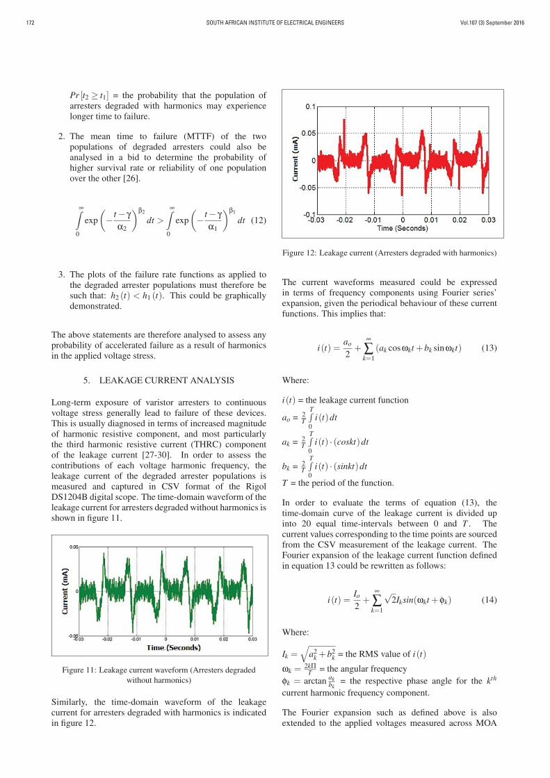
Vol.107 (3) September 2016SOUTH AFRICAN INSTITUTE OF ELECTRICAL ENGINEERS172
Pr [t2 ≥ t1] = the probability that the population ofarresters degraded with harmonics may experiencelonger time to failure.
2. The mean time to failure (MTTF) of the twopopulations of degraded arresters could also beanalysed in a bid to determine the probability ofhigher survival rate or reliability of one populationover the other [26].
∞∫
0
exp(− t − γ
α2
)β2
dt >∞∫
0
exp(− t − γ
α1
)β1
dt (12)
3. The plots of the failure rate functions as applied tothe degraded arrester populations must therefore besuch that: h2 (t) < h1 (t). This could be graphicallydemonstrated.
The above statements are therefore analysed to assess anyprobability of accelerated failure as a result of harmonicsin the applied voltage stress.
5. LEAKAGE CURRENT ANALYSIS
Long-term exposure of varistor arresters to continuousvoltage stress generally lead to failure of these devices.This is usually diagnosed in terms of increased magnitudeof harmonic resistive component, and most particularlythe third harmonic resistive current (THRC) componentof the leakage current [27-30]. In order to assess thecontributions of each voltage harmonic frequency, theleakage current of the degraded arrester populations ismeasured and captured in CSV format of the RigolDS1204B digital scope. The time-domain waveform of theleakage current for arresters degraded without harmonics isshown in figure 11.
Figure 11: Leakage current waveform (Arresters degradedwithout harmonics)
Similarly, the time-domain waveform of the leakagecurrent for arresters degraded with harmonics is indicatedin figure 12.
Figure 12: Leakage current (Arresters degraded with harmonics)
The current waveforms measured could be expressedin terms of frequency components using Fourier series’expansion, given the periodical behaviour of these currentfunctions. This implies that:
i(t) =ao
2+
∞
∑k=1
(ak cosωkt +bk sinωkt) (13)
Where:
i(t) = the leakage current function
ao = 2T
T∫0
i(t)dt
ak = 2T
T∫0
i(t) · (coskt)dt
bk = 2T
T∫0
i(t) · (sinkt)dt
T = the period of the function.
In order to evaluate the terms of equation (13), thetime-domain curve of the leakage current is divided upinto 20 equal time-intervals between 0 and T . Thecurrent values corresponding to the time points are sourcedfrom the CSV measurement of the leakage current. TheFourier expansion of the leakage current function definedin equation 13 could be rewritten as follows:
i(t) =Io
2+
∞
∑k=1
√2Iksin(ωkt +φk) (14)
Where:
Ik =√
a2k +b2
k = the RMS value of i(t)
ωk =2kΠ
T = the angular frequencyφk = arctan ak
bk= the respective phase angle for the kth
current harmonic frequency component.
The Fourier expansion such as defined above is alsoextended to the applied voltages measured across MOA

Vol.107 (3) September 2016 SOUTH AFRICAN INSTITUTE OF ELECTRICAL ENGINEERS 173
samples during degradation test. This yields the followingvoltage expression:
v(t) =Vo
2+
∞
∑k=1
√2Vksin(ωkt +θk) (15)
Where:
Vk =√
a2k +b2
k = the RMS value of v(t)
ωk =2kΠ
T = the angular frequencyθk = arctan ak
bk= the respective phase angle for the kth
voltage harmonic frequency component.
Since the power losses resulting from distorted voltageacross MOA units could be estimated by the sum powerlosses of each components [31]. The instantaneouspower p(t) could therefore be expressed as the product ofequations (14) and (15). Disregarding the dc componentsin both (14) and (15), the following equation is obtained:
p(t) =∞
∑k=1
√2Iksin(ωkt +φk) ·
√2Vksin(ωkt +θk) (16)
Where:
p(t) = the instantanous power.
Developing further equation (16) yields the active orresistive component (PR) of the total power absorbed bythe arrester:
PR =∞
∑k=1
VkIkcos(θk −φk) (17)
Where:
PR = the average power.
The magnitude of the fundamental and harmonic resistivecomponents constituting the leakage currents could beeffectively determined using the expression Ikcos(θk −φk).The fundamental, the third and fifth harmonic resistivecurrent components are shown in figure 13.
6. RESULTS AND DISCUSSION
Based on the mean U − I characteristic curve obtained,arrester population degraded with harmonics proved tohave the lowest decrease (100V ) in the reference voltage(Un) measured at 1 mA dc and at room temperature.Whereas arresters degraded without external source ofharmonics have experienced a decrease of about 150 Vin the reference voltage. This implies that the electricalstability of arresters degraded with harmonics is severelycompromised as shown in figure 7. Based on the
Figure 13: Resistive Current Components before and afterharmonics
conditions of failure stated above, it could be observed that61.67 % of the MOA population degraded with externalharmonics in the voltage stress experienced breakdown,as compared to 45% when the voltage stress contains noexternal harmonic. This could further be observed interms of the hasard or failure rate functions obtained. Thefailure rate function of arresters degraded without externalharmonics h1 (t) is observed to be sharply increasing from0 to 2.46 × 10⁻⁴ failures per hour in the time intervalt ∈ [100.6;500], before decreasing from 2.46 × 10⁻⁴ to2.35× 10−4 failures per hour across the time interval t ∈[500;4500]. For arrester samples degraded with externalharmonics, the failure rate function h2 (t) is observed tobe sharply increasing from 0 to 3.33× 10⁻⁴ failures perhour across the time interval t ∈ [100.6;500]. Across thetime interval t ∈ [500;4500], the failure rate h2 (t) indicateda lower rate increase from 3.33 × 10⁻⁴ to 4.16 × 10⁻⁴
failures per hour. The decreasing failure rate impliesearly failure of arrester components in the life cycleof these components under standard service condition,while the increasing failure rate suggests a wear out ofthese protective devices. This therefore indicates that forthe time-interval [100.6,4500], the failure rate arrestersdegraded without external harmonics is consistently lowerthan that of samples subjected to harmonics. This impliesthat the statement: h2 (t) < h1 (t), for t = [100.6;4500] isnot true and the opposite statement: h1 (t) < h2 (t), for t= [100.6;4500] is therefore true. The failure rate graphsh1(t) and h2(t) are shown in figure 14.
Figure 14: Failure rate function before and after harmonics
An analysis of the reliability function or the survival prob-ability graphs obtained across [100.6;4500] time-interval,for both observed populations shows that R1 (t) decaysfrom 100 % to 36 %, while R2 (t) changes from 100 %

Vol.107 (3) September 2016SOUTH AFRICAN INSTITUTE OF ELECTRICAL ENGINEERS174
to 17 %. Moreover, for each point in time belongingto interval [100.6;4500], it is observed that R1 (t) isconsistently less than R2 (t). Therefore, the lowerreliability or probability of survival for arresters degradedwith external harmonics, as compared to those degradedwith no external harmonics can be associated to the contentof harmonic distortion in the voltage stress. This impliesthe relationship: R1 (t) > R2 (t), for t = [100.6;4500].The reliability functions of both populations are plotted infigure 15.
Figure 15: Reliability functions
The probability of one population of tested arresters toexperience longer time to failure over the other, such asdetermined in equation 11, yields the probability value(Pr = 0.4107 or 41.07%), which is obviously less than0.50 or 50%. This suggests that the time to failure or theprobability of arresters, subjected to external harmonics,experiencing longer time to failure than those degradedwith harmonics is 41.07%. Since the probability sum:Pr [t2 ≥ t1] + Pr [t1 ≥ t2] = 1. This therefore impliesPr [t1 ≥ t2] = 1 - Pr [t2 ≥ t1] = 0.5893 or 58.93%. Thissuggests that the stated relationship: P [t2 ≥ t1] > 0.50cannot be true, and consequently the probability ofarresters, degraded without external harmonics, to survivelonger is actually 58.93% higher.The MTTF obtained for arresters degraded withoutharmonics is found to be 4252.65 hours as opposed to2512.81 hours for those degraded with external harmonics.This demonstrates that metal oxide arresters degraded withexternal harmonics experienced 40.91% reduction of theirlifetime, and therefore demonstrated lower reliability.The PDF curves obtained in figure 16 show higher densityof failure for the arrester components subjected to externalharmonics. The magnitude of the fundamental, the 3rd and5th harmonic resistive current components obtained are:0.013 mA, 0.005 mA, 0.003 mA for arresters degradedwithout harmonics and 0.137 mA, 0.104 mA, 0.082 mAfor those degraded with external harmonics, respectively.The resistive current component before harmonic injectionis therefore 0.0143 mA and 0.191 mA after injectionof external harmonics. An increase of 92.51% in theresistive current of the arrester samples degraded in thepresence of external harmonics was therefore observed.
Figure 16: PDF of degraded arrester populations
It could also be noted that the fundamental and theTHRC make up at least 90% of the total resistive currentmeasured before and after harmonics injection at thesame operating temperature. This shows correlationbetween the increase in the resistive current and thehigher probability of failure, the reduced MTTF, thehigher failure rate and lower reliability as well as thesevere shift in the U − I characteristic curve, in arresterpopulations subjected to external harmonics. The increasein the resistive current directly translates into increasedpower losses being absorbed by arrester components,which will therefore quicken the thermal runway process.Since the test temperature which represents the device’soperating environment was kept constant, the rise in theresistive current and the subsequent high power lossesexperienced, when external harmonics are injected, couldtherefore be attributed to the influence of harmonic voltagefrequencies on the overall continuous biasing effect ofthe applied voltage stress. Furthermore, the study onthe degradation mechanism of metal oxide-based arrestersdescribed in [4], revealed that the degradation of thesearresters consists of the resultant effect of the breakdownof several millions of individual grain boundaries atthe following voltage levels: 3.02 V and 3.11 V pergrain boundary, for monotonous and non-monotonousageing process respectively. This therefore suggests thatthe reduced time to failure and the increased resistivecurrent, observed in MOA samples subjected to externalharmonics injection, results from the contributing effect ofvoltage harmonic components on the breakdown voltagebetween individual grain boundaries. This demonstratesthat voltage harmonics could be regarded as aggravatingfactors of the long-term degradation phenomenon of theseovervoltage protective devices. The third harmonic voltagewill, by virtue of its magnitude, be the second voltagecontributor to the MOA microstructure disintegration,hence to the accelerated degradation.
7. CONCLUSION
For the purpose of this work, similar arrester units aresubjected to accelerated degradation test, at elevatedtemperature and voltage. The voltage applied is embeddedwith harmonics. The observed time to failure or lifeexpectancy represents the behaviour pattern of these

Vol.107 (3) September 2016 SOUTH AFRICAN INSTITUTE OF ELECTRICAL ENGINEERS 175
overvoltage units, when operating at normal servicecondition with distorted voltage for a long period of time.The resistive current components as well as the U − Icharacteristic curve confirm the the degradation status ofarrester units. The following findings are obtained:
1. Continuous exposure of metal oxide-arresters todistorted ac voltage is prone to aggravate thedegradation or failure process of these surgeprotection units.
2. The reduced time to failure or lifetime of MOA units,continuously operated under distorted ac voltage,could be attributed to additional watt loss experiencedin these devices which result from increased harmonicresistive current conduction.
3. Harmonic components embedded in the voltage stresscontribute to the biasing effect of MOA units.
These findings imply that the presence of harmoniccomponents in the voltage across arrester units willfast track the disintegration process of the intergranularboundaries of MOA arresters. This therefore explainsthe higher probability of electrical failure or reduced lifeexpectancy of metal oxide-based arresters under harmonicdistortion conditions. The develpment of new oxideadditives, capable to decelerate intergranular disintegrationunder the effect of voltage stress, could be recommendedas one of the directions for future designs of MOAs.
REFERENCES
[1] A. Vasic, M. Vujisic and P. Osmokrovic: “Aging ofovervoltage protection elements caused by past ac-tivations”, Microelectronics, Electronic Componentsand Materials, Vol. 42 No. 3, pp. 197-204, October2012.
[2] K. Eda, A. Iga and M. Matsuoka: “Degradationmechanism of non-ohmic zinc oxide ceramics”,Journal of Applied Physics, Vol. 51 No. 5, pp.2678-2684, January 1980.
[3] D. Zhou, C. Zhang and S. Gong: “Degradationphenomena due to dc bias in low-voltage ZnOvaristors”, Materials Science and Engineering:B,Vol. 99 No. 1-3, pp. 412-415, May 2003.
[4] J. He, J. Liu, J. Hu, R. Zeng and W. Long:“Non-uniform behaviour of individual grain bound-aries in ZnO varistor ceramics”, Journal of theEuropean Ceramic Society, Vol. 31 No. 8, pp.1451-1456, July 2011.
[5] C. Nahm : “Microstructure, electrical properties, andaging behaviour of ZnO-Pr6O11-CoO-Cr2O3-Dy2O3varistor ceramics”, Ceramics International, Vol. 37No. 8, pp. 3049-3054, December 2011.
[6] Z. Nanfa, K. Guoyao and G. Yaping: “Long durationimpulse withstand capability of SPD”, Proceedings:the Asia-Pacific International Symposium on Electro-magnetic Compatibility, Beijing, April 2010.
[7] J. Rossman, J. Nelson and M. Droke: “Reliabilityand failure of porcelain high-voltage surge arresters”,Proceedings: International Conference on HighVoltage Engineering and Application, New Orleans,October 2010.
[8] V. Hinrichsen: “Monitoring of high voltagemetal oxide surge arresters”, Proceedings: 6th
International Conference on Electrical Insulation,Bilbao, October 1997.
[9] M. Jaroszewsky, P. Kostyla and K. Wieczorek:“Effect of voltage harmonics content on arresterdiagnostic result”, Proceedings: InternationalConference on Solid Dielectrics, Toulouse, July2004.
[10] V. Larsen and K. Lien: “In-service testing anddiagnosis of gapless metal oxide surge arresters”,Proceedings: 9th International Symposium onLightning Protection, Foz do Iguacu, November2007.
[11] P. Bokoro, M. Hove and I. Jandrell: “Statisticalanalysis of MOV leakage current under distortedsupply voltage conditions”, Proceedings: IEEEElectrical Insulation Conference, Philadelphia, June2014.
[12] R. Hernandez, I. Ramrez, R. Saldivar and G.Montoya: “Analysis of accelerated ageing ofnon-ceramic insulation equipments”, Generation,Transmission and Distribution, IET, Vol. 6 No. 1, pp.59-68, January 2012.
[13] Nabertherm GmbH: High temperaturelaboratory furnace operating manual,http://www.nabertherm.com. 2011.
[14] IEEE P519.1/D12: Guide for Applying HarmonicLimits on Power Systems, IEEE Power StandardsCoordinating Committee, November 2012.
[15] Lapp Cables Group: High temperature cablesoperating instructions, http://www.lappkabel.co.za.2013.
[16] IEEE 930T M: IEEE guide for the statistical analysisof electrical insulation breakdown data, IEEEStandards 2007.
[17] Epcos data book: SIOV Metal Oxide Varistors, pp.51-52, http://www.epcos.com. 2008.
[18] M.Wang, Q.Tang, and C.Yao: “Electrical propertiesand ac degradation characteristics of low voltageZnO varistors doped with Nd2O3”, CeramicsInternational, Vol. 36 No. 3, pp. 1095-1099, January2010.

Vol.107 (3) September 2016SOUTH AFRICAN INSTITUTE OF ELECTRICAL ENGINEERS176
[19] J. He, J. Liu, J. Hu, and W. Long: “AC ageingcharacteristics of Y2O3-doped ZnO varistors withhigh voltage gradient”, Materials Letters, Vol. 65 No.17-18, pp. 2595-2597, September 2011.
[20] IEEE C62.11: IEEE standard for metal oxide surgearresters for ac power circuits higher than 1 kV,IEEE Standards 1999.
[21] J. White : “The moments of log-Weibull orderstatistics”, Techtometrics, Vol. 11 No. 2, pp. 373-386,February 1969.
[22] H. Yahyaoui, P. Notingher, S. Angel andY. Kieffel: “Proprietes dielectriques d’uneresine epoxy d’alumine sous l’effet du champelectrique continu et de la temperature”,Proceedings: Journees JCGE’ 2014-SEEDS,http://www.hal.archives-ouvertes.fr/hal-01083915,June 2014.
[23] P. D. O’connor and A. Kleyner: Practical Reliability,John Wiley and Sons, UK, fifth edition, chapter 3, pp.87-92, August 2011.
[24] A. S. Yahaya, C. S. Yee, N. A. Ramli and F.Ahmad: “Determination of the best probabilityplotting position for predicting parameters ofthe weibull distribution”, International Journal ofApplied Science and Technology, Vol. 2 No. 3, pp.106-112, March 2012.
[25] G. G. Brown and H. C. Rutemiller: “Evaluation ofPrX ≥ Y when both X and Y are three-parameterweibull distributions”, IEEE Transactions on Relia-bility, Vol. R.22 No. 2, pp. 78-82, June 1973.
[26] M. Kayid, I. A. Ahmad, S. Izadkhah and A. M.Abouammoh: “Further results involving the meantime to failure order, and the decreasing mean time tofailure class”, IEEE Transactions on Reliability, Vol.62 No. 3, pp. 670-678, September 2013.
[27] C. Karawita and M. Raghuveer: “Leakage currentbased assessment of degradation of MOSA usingan alternative technique”, Proceedings: AnnualReport of the Conference on Electrical Insulation andDielectric Phenomena (CEIDP), October 2005.
[28] Z. Abdul-Malek, N. Yusof and M. Yousof: “Fieldexperience on surge arrester condition monitoringmodified shifted current method”, Proceedings: 45th
Universities Power Engineering Conference (UPEC),Cardiff, 2010.
[29] X. Yan, Y. Wen and X. Yi: “Study on theresistive leakage current characteristic of MOV surgeArresters”, Proceedings: Asia-Pacific IEEE/PESTransmission and Distribution Conference andExhibition, Yokohama, October 2002.
[30] M. Khodsuz, M. Mirzaie and S. Seyyedbarzegar:“Metal oxide surge arrester condition monitoringbased on analysis of leakage current components”,
International Journal of Electrical Power and EnergySystems, Vol. 12 No. 6, pp. 188-193, November 2014.
[31] E. Shulzhenko, M. Rock, M. Birle and C.Leu: “Applying of surge arresters in powerelectronic network components”, Proceedings: theInternational Conference on Lightning Protection,Shanghai, October 2014.

Vol.107 (3) September 2016 SOUTH AFRICAN INSTITUTE OF ELECTRICAL ENGINEERS 177
RAINFALL RATE AND ATTENUATION PERFORMANCE ANALYSIS AT MICROWAVE AND MILLIMETER BANDS FOR THE DESIGN OF TERRESTRIAL LINE-OF-SIGHT RADIO LINKS IN ETHIOPIA F. D. Diba*, T. J. Afullo ** and A. A. Alonge *** *Discipline of Electrical, Electronics and Computer Engineering, University of KwaZulu-Natal, Durban 4041, South Africa, email: [email protected] **Discipline of Electrical, Electronics and Computer Engineering, University of KwaZulu-Natal, Durban 4041, South Africa, email: [email protected] ***Discipline of Electrical, Electronics and Computer Engineering, University of KwaZulu-Natal, Durban 4041, South Africa, email: [email protected] Abstract: Rainfall is a major cause of propagation degradation in wireless communication systems at microwave and millimetre bands. While the International Telecommunications Union (ITU-R) recommends rain attenuation models based on measured rainfall and radio propagation data, the propagation model in Ethiopian context remains unstudied - with one-minute rainfall rate measurement recommended by ITU-R also unavailable. This paper thus addresses the following: the estimation of the cumulative probability distribution, giving the rainfall rate versus the percentage of time the indicated rainfall was exceeded in a year; derivation of one-minute rain rate distribution using the Rice-Holmberg (R-H) model, and then proposing the rainfall rate conversion factors for Ethiopian sites from 15-minute to one-minute integration time; developing rain rate and fade margin contour maps for Ethiopia; and modelling rain attenuation using the ITU-R method. Key words: Ethiopia Link Design, Rain rate, conversion factor, contour map, rain attenuation.
1. INTRODUCTION
The fast growth in wireless networks is leading to the saturation of the lower frequency bands (1-10 GHz).This reality has shifted emphasis to the higher frequency spectrum, especially in the region 30-100 GHz. However, atmospheric effects, especially rain is a dominant cause of signal degradation at microwave and millimetre bands, which leads to network outages. Rain attenuation is noticeable from propagation frequency above10 GHz in the temperate zone, while in tropical climate its effect is felt from 7 GHz [1]. When a microwave or millimetre wave signal travels through a rainy medium, its strength drastically weakens owing to the effect of absorption and scattering by rain drops on its amplitude and phase components [2]. In addition, rain droplets alter the polarization of the transmitted signal, resulting in depolarization effects at the receiver. Thus current microwave transmission network design needs detailed knowledge of rainfall attenuation, depolarization, and fades depth to meet the quality and reliability specifications for optimum system capacity [3]. In practice, the parameters of rainfall rate and raindrop size are investigated to improve the understanding of rainfall effects over wireless communications [4]. The study of radio wave propagation in the microwave and millimetre bands is of immense interest to both the International Telecommunications Union (ITU-R) and the International Union of Radio Science (URSI). The ITU-R, through recommendations P530-15 [5] and P618-11 [6], provides basic Line-of-Sight (LOS) link design
assumptions based on propagation prediction methods which are seldom suitable for tropical regions. It is, therefore, imperative for these regions to determine the parameters experimentally with a view to modify the ITU-R propagation prediction methods. Many researchers have studied the clear-air and rain effects on radio links in Southern Africa [7-13], Nigeria [14], and other tropical countries such as Malaysia [15] and Bangladesh [16]. However, many tropical and equatorial African regions have not been adequately studied. As a case in point there have been no investigative studies on rain attenuation effects at microwave and millimetre bands in Ethiopia. In this work, a 15 minute sampling time rain rate (R15min) cumulative distribution computed, giving the rainfall rate versus the percentage of time the indicated rainfall was exceeded in a year for several regions of Ethiopia based on data obtained from National Meteorological Agency (NMA) of Ethiopia. As one-minute integrated rainfall data is not available for Ethiopia, the measured rainfall rate was converted from the higher integration time (15 minutes in this case) to one-minute integration time, using the Rice-Holmberg (R-H) method [17]. These rainfall rate distributions were developed for ten Ethiopian locations, namaly: Addis Ababa, Adama, Arbaminch, Bahirdar, Diredawa, Dubti, Jimma, Kombolcha, Mekele and Negelle Borenna. Thereafter, a general conversion factor for the rest of the country’s locations is proposed. In addition, contour maps for rainfall rate and fade margin are developed and analysed for sites throughout Ethiopia. Based on ITU-R recommendation in [5], the specific rain attenuation for

Vol.107 (3) September 2016SOUTH AFRICAN INSTITUTE OF ELECTRICAL ENGINEERS178
frequency range of 1-300 GHz is determined in this project. Moreover, path attenuation of rainfall rate versus operation frequencies for different path lengths are estimated. Finally, regarding rainfall attenuation, it is noted that Sami Sharif [20] has done the closest work over Sudan, bordering western Ethiopia.
2. GEOGRAPHY AND CLIMATE OF ETHIOPIA
Geographically, Ethiopia is located between latitudes 30N to 180N, and longitudes 330E to 480E, with an altitude
variation from 100 meters below sea level to over 4000 metres above sea level. It is surrounded by Eritrea to the north, Djibouti to the north-east, Somalia to the east and south-east, Kenya to the south, and Sudan to the west, as shown in Fig.1. Ethiopia is generally a country of plateaus, with the Great Rift Valley separating the western and eastern highlands. The highlands slowly slope to the lowlands of Sudan to the west and Somalia to the east. The climate of the Ethiopian highlands is temperate, and of the lowlands is hot [18]. Over Ethiopia, the climatic variations tend to depend on unique features of the area. The classification of climate by Köppen (proposed in 1931), which is based on geographical elevation, was found useful in this case [19]. Thus, the three main climate classifications in Ethiopia are Class A (As, Aw (tropical), Am) climates of lowlands, varying from semi-humid to semi-arid surrounds the highlands; Class B (BWh (hot-arid), BSh (hot-semi arid) and BSk) climate in the Afar-Triangle and the Somali Region; and class C (Cwb (warm temperate), Cfb (warm temperate), Cwc) climates in the highlands, ranging from warm to cool mountains with semi-humid to humid characteristics.
3. RAIN MEASUREMENT AND DATA
PROCESSING
The cumulative distribution of rainfall rate (Rp) presents the rain intensity versus percentage of the time (over one year) (p) the indicated rain rate is exceeded. ITU-R [21] requires calculation of R0.01 mm/h to predict the attenuation due to rain. R0.01 occurs at 0.01% of the time exceedance, which can be read from the ITU-R map [21] or obtained from long-term local measurements. The parameter relies on the integration time of the rainfall measuring devices used. According to [14] and [22], the most desired integration time is one minute. Since one-minute rainfall data is unavailable in Ethiopia, converting from higher integration times to one-minute integration time is therefore required. Therefore Section 3.1 covers measurement and data processing; while section 3.2 covers 15 minute integration time rainfall distribution. 3.1 Rain Measurements and Data Processing Different devices are available to record rainfall. The NMA of Ethiopia uses two techniques to collect rain data, namely, it applies networks of rain gauges to measure rainfall intensity every 24 hours, and automated rain gauges to record rainfall intensity per 15 minute. The gauges meet the World Meteorological Organization standards. For the purpose of this paper, three years raw rainfall data collected by NMA comprising rainy and non-rainy (zero value) days is considered. Only the rain intensities with values different from zero were sorted out and processed, and then the appropriate mathematical formulation was used to calculate the required parameters.
Figure 1: Map of Ethiopia
Table 1: Locations and their climate in Ethiopia
Location Lat. (ON)
Long. (OE)
Accum. M(mm)
Köppen Class
Addis Ababa 9.02 38.45 1089 Cwb Adama 8.33 39.17 904.2 Aw Arbaminch 6.03 37.33 820 Aw Bahirdar 11.35 37.23 1480 Cwb Dire Dawa 9.58 42.32 729.8 BSh Dubti 11.73 41.08 300 Bwh Jimma 7.40 36.49 1414 Cfb Kombolcha 11.09 39.74 1139 Cwb Negele 5.33 39.58 550 Aw Mekele 13.28 39.32 601 Bsh Table 2: R15min (mm/h) values being exceeded at 1%, 0.1% and 0.01% of the time in a year Locations
Rain Rate (mm/h)
1% 0.1% 0.01% Addis Ababa 1.5 5.5 13
Adama 1.8 7.5 18 Arbaminch 1.7 6.5 17 Bahir Dar 2.3 10.5 23.6 Dire Dawa 1.3 5 13.5 Dubti 0.2 2.5 8.5 Jimma 2.2 13 21.5 Kombolcha 5 11 20.5 Negele 1.3 5.6 11 Mekele 1.4 5.8 13.5

Vol.107 (3) September 2016 SOUTH AFRICAN INSTITUTE OF ELECTRICAL ENGINEERS 179
3.2 15- minute Rainfall Rate Distribution in Ethiopia The cumulative rainfall rate distribution for ten locations in Ethiopia is calculated and plotted based on the data from NMA of Ethiopia at 15 minute integration time. Figure 2 shows rain rate distribution for ten main sites of Ethiopia versus percentage of exceedance of time of the year for the 15 minute sampling rate. From Figure 2 and Table 2 the maximum value of rain rate R0.01 (R at 0.01%) is 23.6 mm/h observed at Bahirdar, while the minimum value of R0.01 is 8.5 mm/h, recorded at Dubti.
4. MODELING OF ONE-MINUTE RAINFALL RATE
CUMULATIVE DISTRIBUTION (CD)
There exist a number of rain rate distribution models for one-minute integration time. Some of these models include the Rice-Holmberg (R-H) model [17], the Kitami model [23], the Moupfouma model [24], and the Global ITU-R model [21]. The R-H model depends on the average annual precipitation and the thunderstorm ratio as the two vital parameters for estimating the rain rate from the local rain data. These parameters can either be obtained from the maps presented in [22] or estimated from the long-term average annual precipitation, the number of thunderstorm days, and the maximum monthly precipitation. The Kitami model was proposed by Ito and Hosoya [23], and it is based on two regional climatic parameters namely: the thunderstorm ratio and the average annual precipitation. Moupfouma’s model, developed by Moupfouma and Martin, offers a simple approach to the prediction of rain rate distribution for both temperate and tropical climates. Considering the variability of all the rain rate predictions, the R-H model has been determined to give a much better performance than others [25]. Hence, Section 4.1 presents the R-H rain
rate distribution model, section 4.2 discusses the conversion factors of rainfall rate from 15 minute to one–minute integration time, and section 4.3 discusses the development of the rain rate contour map. 4.1 Rice Holmberg rainfall distribution model In this work, the Rice-Holmberg model is used to determine one-minute rainfall rate cumulative distribution (CD) from local meteorological data to generate the two main parameters of distribution prediction, which are the average annual accumulated rainfall data (M), and thunderstorm ratio β. The average rainfall accumulation (M) is the sum of the thunderstorm accumulation (M1) and all other rain (M2), where:
21 MMM (1)
The thunderstorm ratio is defined as:
MM1
(2)
The number of hours of rain at one-minute periods (T1(R)) for which a surface point rainfall is exceeded is given by [17]:
]63.1exp86.1258.0[exp12.0
03.0exp03.01
RRRMRT
(3)
Hence, the percentage of time of an average year during which one-minute average rainfall rates exceed is
66.87% 1 RTP
In this work, the parameter M is measured by NMA of Ethiopia, whereas β is obtained from the map in [17], which is 0.2 for Ethiopia. Figure 3 shows the calculated R-H one minute integration time of rain rate distribution versus percentage of time exceedance for ten locations in Ethiopia. From the figure, the maximum rain rate (R) at 0.001%, 0.01%, and 0.1% of exceedance of time is in Bahirdar, while the minimum is recorded in Dubti as the values listed in Table 3 below. 4.2 Determination of Rainfall Rate Conversion Factors over Ethiopia The 15 minute rain intensity data for Ethiopian locations were obtained from the NMA of Ethiopia for a period of three years. The rainfall rate conversion from higher integration time to a smaller integration time has been
Figure 2: Cumulative rain rate distribution at 15 minute
sampling rate in Ethiopia

Vol.107 (3) September 2016SOUTH AFRICAN INSTITUTE OF ELECTRICAL ENGINEERS180
developed by many researchers [11, 22, and 24]. ITU-R P 837.6 also presents the power-law empirical conversion method for some countries, and regional maps exist
showing regional values for R0.01. The methods of Flavin [26], Segal [27], and Singh et al [28], are also based on the power-law conversion approach.
Segal developed conversion factors, p , for converting rain intensity data having an integration time of minutes to equivalent one-minute rainfall rates, as given by [27]:
pRpRp
1
(4)
where R1 and Rτ are the rainfall rates exceeded with equal probability P, for the two integration times [27]. The factor (P) is also given by the power law [28]:
bapp (5)
where P is the probability of occurrence, and a and b are the regression coefficients derived from the measured rainfall data. From Table 4, the general conversion factor for Ethiopia is given by:
4805.1151 )(199.1 pRpR (6)
Figure 4 shows the conversion factor graph for only two locations (Adama and Jimma) with their corresponding regression and correlation coefficients. 4.3 Contour Mapping of Rainfall Rate Distribution for Ethiopia In this study, the rain rates at 0.01% of time exceedance is calculated from available data for ten stations in Ethiopia. However, there is need to determine R0.01 for all locations in the country. Using spatial interpolation techniques, the unknown points all over Ethiopia are estimated. There are a number of spatial interpolation methods, such as kriging, inverse distance weighting (IDW), thin-plate spline, multiqudric, and bi-linear. From the above spatial interpolation techniques, IDW is the simplest and performs best [13, 29] and, thus, IDW is used in this work. IDW considers that the nearby values weight more to the interpolated points than the distance observations (that means the contribution of known data points are inversely proportional to the distance from the unknown location that is being predicted). The IDW expression is given by [30]:
m
N
mmn ZZ
1 (7)
Figure 3: R-H rainfall rate cumulative distribution at
one minute integration time in Ethiopia
Table 3: R1min (mm/h) for 99%, 99.9%, 99.99% availability
Locations Rain rate values at 0.1%,0.01% and 0.001% of time in a year
0.1% 0.01% 0.001% Addis Ababa 14 64 140 Adama 12 60 138 Arbaminch 11.5 58 134 Bahir Dar 17 76 155 Dire Dawa 10.5 53 130 Dubti 8 28 100 Jimma 16 73 152 Kombolcha 13.5 63.5 142 Negele 10 44 120 Mekele 10.2 46.5 123
Table 4 Values for regression and correlation coefficients for conversion factors
LOCATION a b R2
Addis Ababa 15 1.44 1.507 0.945
Adama 15 0.919 1.435 0.991
Arbaminch 15 0.926 1.435 0.962
Bahir dar 15 1.088 1.316 0.976
Dire Dawa 15 0.906 1.619 0.965
Dubti 15 8.263 0.738 0.817
Jimma 15 1.182 1.593 0.981
Kombolcha 15 1.492 1.441 0.958
Mekele 15 0.964 1.498 0.979

Vol.107 (3) September 2016 SOUTH AFRICAN INSTITUTE OF ELECTRICAL ENGINEERS 181
N
m mmm dd 1
11 (8)
11
N
mm (9)
22nmm yyxxd (10)
Here, Zn is the estimated value at point n, Zm is the observed value at the sample point m, ωm is the weight allocated to the sample points, N indicates the number of sample points, dm is the distance between m and n, β is the power parameter and (x; y) are the coordinates of the interpolation point and (xm; yn) are the coordinates of the sample points. We use two different types of software, namely, PAST version 2.17C, and MATLAB. PAST is a free software tool and it is a package used for statistical data analysis, plotting and modelling functions. Interpolation of data was done using PAST and plotting of contour maps was carried out in MATLAB. Figure 5 shows the proposed rainfall rate distribution contour map of Ethiopia of R0.01 using the R-H model. It is seen from the figure that the western and central high lands part of Ethiopia experience higher rainfall rate distribution than the eastern low lands as expected.
5. DETERMINATION OF RAIN ATTENUATION OVER ETHIOPIA
Rainfall that occurs over terrestrial radio links induces attenuation because of the electromagnetic wave scattering and absorption by rain drop particles. In order to characterize rain attenuation, ITU-R (530-15) proposed a rainfall attenuation prediction model. Therefore, Section 5.1 discusses the specific attenuation while Section 5.2 presents total rain attenuation for varying path length and frequency.
5.1 Determination of Specific Attenuation of Rainfall The attenuation due to rain for terrestrial radio links is based on R0.01, signal polarization, propagation frequency, and path length. The first step is to determine the specific rain attenuation - that is, rain attenuation per kilometre in a rainy medium. In this paper, the value of R0.01 is computed using R-H model as shown in Table 3. However, if local data is not available, R0.01 can be estimated from the ITU-R map in [21]. The specific attenuation (dB/km) is given by [31]:
01.0KRR (11)
Here R is specific attenuation, K and α are the regression coefficients which are determined as a function of frequency as given in [31] for horizontal and vertical polarization. Figures 6a and 6b show the calculated distribution of specific attenuation of rain versus frequency for ten locations in Ethiopia, namely: Addis Ababa, Adama, Arbaminch, Bahirdar, Diredawa, Dubti, Jimma, Kombolcha, Mekele and Negele Borena. In fact, these are typical locations that represent most parts of the country. Figure 6a shows the specific rain attenuation for horizontal polarization for the ten locations; while Figure 6b is for vertical polarization. Fig.6 shows the fast increase of specific attenuation for frequency ranges up to
Figure 4: 15- minute to 1-minute conversion for
Adama and Jimma
Figure 5: Contour map of rain rate using R-H model at 0.01% for Ethiopia

Vol.107 (3) September 2016SOUTH AFRICAN INSTITUTE OF ELECTRICAL ENGINEERS182
50 GHz, then a more gradual increment from 50 to 100 GHz. These values then remain practically constant for frequencies up to 150 GHz. Finally, it slowly decreases for the rest of propagation frequency. It is seen from Figure 6a that the maximum specific attenuation of 22 dB is observed in Bahirdar, while the minimum of 10 dB is estimated in Dubti at 50 GHz. From Figure 6b, the highest specific rain attenuation of 20 dB is observed in Bahirdar, while the lowest (8 dB) is observed in Dubti at the frequency of 50 GHz. From Figure 6 it is also seen the specific rain attenuation for horizontal polarization is higher than for vertical polarization, because of the fact that the raindrops have a non-spherical shape with flattened base and therefore, the horizontally polarized waves are attenuated more than the vertically polarized waves.
5.2 Determination of Rainfall Attenuation
According to the ITU-R model [5], the prediction of rainfall attenuation involves the following five steps: Step 1: Determination of the rain rate (R0.01), as seen in Table 3 and Figure 3. Step 2: Computation of specific attenuation R (dB/km), as given equation (11) above. Step 3: Calculation of the effective path length (deff) of the link which can be computed by multiplying the actual path length (d) with the distance factor r, where r is given by [5]:
dfRdr
024.0exp1579.10477.01
123.0073.001.0
633.0
(12)
Here, f is the frequency (GHz), α is the regression constant in specific attenuation, and r is less than or equal to 2.5. Step 4: Estimation of path attenuation that is exceeded 0.01% of time is given by [5]:
drA R01.0 (13) Step 5: Computation of rain attenuation for different percentages of exceedance in the range 0.001% to 1% as given by [5]:
pCCp PCAA 1032 log
101.0 (14)
00 11 12.007.0 CCC (15)
]1[546.0855.0 002 CCC (16)
]1[043.0139.0 003 CCC (17)
GHzf
GHzffC
1012.0
1010
log4.012.08.0
100
(18)
Fig. 6(a)
Fig. 6(b)
Figures 6a and b: Specific rain attenuation for
Ethiopia versus frequency for horizontal and vertical polarization

Vol.107 (3) September 2016 SOUTH AFRICAN INSTITUTE OF ELECTRICAL ENGINEERS 183
The prediction procedure outlined above is considered to be valid in all parts of the world at least for frequencies up to 100 GHz and path lengths up to 60 km [5]. Figures 7a and 7b show the rain attenuation versus link path length for horizontal and vertical polarizations for ten sites in Ethiopia over different distances. From these graphs, the rain attenuation rises sharply for the first 20 km, then increases less sharply from 20 km to 40 km and finally the attenuation settles almost to a constant. As the distance increases, the rain attenuation becomes non-uniform because of the fact that for large actual path lengths, the effective path length remains fixed. As seen in Figure 7a with horizontal polarization at distance of 20 km, the maximum rain attenuation is observed at Bahirdar at 41 dB, while the minimum is at Dubti at 16.2
dB. For vertical polarization (Figure 7b) similar distribution of rain attenuation is observed: the highest value is 35 dB in Bahirdar, and lowest value is 14.5 dB in Dubti at 20 km. comparing the two graphs, vertical polarization has lower rain attenuation than horizontal polarization, as already stated. Rainfall occurs some times of the year with varying rates from time to time, hence the rain fade margin needed to compensate for rain attenuation varies with time. Figures 8a and 8b show the fade depth at various percentages of time. Figure 8a gives the attenuation values for horizontal polarization at different percentages of time at 13 GHz and 13.34 km path length. At 0.01% of the time (99.99% availability), the maximum fade depth is 31.14 dB as observed in Bahirdar while the minimum is 12.25 dB recorded in Dubti. For vertical polarization (Figure 8b) similar distribution of rain fade is observed: the highest value is 26.25 dB in Bahirdar, and the lowest value is 10.97 dB in Dubti at the same link distance and operating frequency. Comparing the two graphs, vertical polarization has 14% lower rain attenuation than horizontal polarization.
From the rain attenuation distribution plots shown in Figures 8a and 8b above, fade margin values are determined at different percentages of time of the year for the ten geographical locations. Tables 5 and 6 give the required fade margins at 13 GHz and 13.34-km path length for the ten geographical locations in Ethiopia. The reference link availabilities are 99.999%, 99.99%, 99.9% and 99%. As seen from Tables 5 and 6, the rain fade decreases as availability reduces from 99.999% to 99%. Figures 9a and 9b show rainfall fade margin contour maps for horizontal and vertical polarization, respectively. As seen from the maps, the fade margin decreases as we move from the western to the eastern part of the country, and horizontal polarization requires a higher fade margin than vertical polarization
6. CONCLUSION In this work, the rainfall rate distributions for ten geographical locations in Ethiopia are determined at 15-minute sampling rain rate. The R-H model is then used to convert the local measurement of annual rainfall accumulation into one-minute integration time rain rate distribution. Also, the rainfall rate and fade margin contour maps at 0.01% exceedance are developed for Ethiopia. Using the ITU-R model, specific rain attenuation and total rain attenuation for terrestrial Line-of-Sight links in Ethiopia are predicted for varying frequencies and distances. It is found that the attenuation for shorter link paths is more affected by rainfall than longer distance due to non-uniformity of rain distribution over the link. In descending order, the attenuation of rainfall rate is the highest in Bahirdar, followed by Jimma, Kombolcha, AddisAbaba, Adama, Arbaminch, Diredawa, Mekele, Negele Borena and least in Dubti. The
Fig. 7(a)
Fig. 7(b)
Figures 7a and b: Attenuation versus distance at 13
GHz for Horizontal and Vertical Polarization respectively

Vol.107 (3) September 2016SOUTH AFRICAN INSTITUTE OF ELECTRICAL ENGINEERS184
data from these maps will be useful as preliminary design tools for terrestrial microwave engineers.
REFERENCES
[1] F. Moupfouma: “Improvement of a rain attenuation prediction method for terrestrial microwave links," IEEE Transactions on Ant. and Prop., Vol. 32, No. 12, pp. 1368-1372, 1984.
[2] R. E. Collin: “Antennas and Radiowave Propagation,” 401-402, McGraw Hill, ISBN 0-07-Y66156-1, 1995
[3] Khandaker Lubaba Bashar, Mohammad Mahfujur
Rashid: “Performance Analysis of Rain Fades on Microwave Earth-to-Satellite Links in Bangladesh.” International Journal of Engineering and Technology Vol. 4, No. 7, July 2014
[4] A. A. Alonge and T.J. Afullo: "Rainfall
Microstructures for Microwave and Millimeter Wave Link Budget at Tropical and Subtropical Sites," IEEE Africon, Le Meridien - Ile Maurice; Mauritius, 09 Sep - 12 Sep 2013.
[5] ITU: "Propagation Data and Prediction Methods
Required for the Design of Terrestrial Line-of-Sight Systems," in Recommendation ITU-R P. 530-15; P Series, Geneva, 2013.
[6] ITU: "Propagation Data and Prediction
MethodsRequired for the Design of Earth-Space Telecommunication Systems," in Recommendation ITU-R P.618-11; P Series, Geneva, 2013.
[7] S.J. Malinga, P.A. Owolawi and T.J.O. Afullo:
"Estimation of Terrestrial Rain Attenuation at Microwave and Millimeter Wave Signals in South Africa Using the ITU-R Model," in PIERS Proceeding, Kuala Lumpur, Malaysia, pp. 952-962, March 27-30 2012.
[8] S. Malinga, P. Owolawi and T. Afullo:
"Determination of Specific Rain Attenuation Using Different Total Cross Section Models for Southern Africa," Johannesburg; Vol. 105, pp. 20-30, March 2014.
[9] S.J. Malinga, P.A. Owolawi and T.J.O. Afullo:
"Computation of Rain Attenuation through Scattering at Microwave and Millimeter Bands in South Africa," in Progress in Electromagnetics Research Symposium Proceedings, Taipe, pp.959-970, March 25-28, 2013
[10] M. O. Fashuyi, P. A. Owolawi, and T. J. Afullo:
Rainfall rate modeling for LOS radio systems in South Africa," South African Institute of Electrical Engineering Journal, Vol. 97, No. 1, pp.74-81, March 2006.
[11] P. O. Akuon and T. J. O. Afullo: “Rain Cell Sizing
for the Design of High Capacity Radio Link Systems in South Africa,” Progress in Electromagnetics Research B, Vol. 35, pp. 263-285, 2011
[12] A. A. Alonge and T. J. Afullo: “Rainfall
Microstructural Analysis for Microwave Link Networks: Comparison at Equatorial and Subtropical
Fig. 8(a)
Fig. 8(b)
Figures 8a and b: Attenuation against exceedance for
13.34 km path distance and 13GHz propagation frequency in HP and VP respectively

Vol.107 (3) September 2016 SOUTH AFRICAN INSTITUTE OF ELECTRICAL ENGINEERS 185
Africa,” Progress in Electromagnetic Research B, Vol. 59, pp. 45 – 58, 2014.
[13] P. A. Owolawi: “Rainfall Rate Probability Density
Evaluation and Mapping for the Estimation of Rain Attenuation in South Africa and Surrounding Islands,” Progress in Electromagnetics Research, Vol. 112, pp. 155-181, 2011.
[14] G. Ajayi and E.B.C. Ofoche: "Some Tropical
Rainfall Rate Characterstics at IIe-Ife for Microwave and Millimeter Wave Applications," in Journal of Climate and Applied Meteorology, Vol. 23, 29 pp. 562-567, November 1983.
[15]U. Kesavan, A.R.Tharek and A. Rahman:
"Comparative Studies of the Rain Attenuation Predictions for Tropical Regions," in Progress in Electromagnetics Research, Vol. 18, pp. 17-30, 2011.
[16] S. Hossain: "Rain Attenuation Prediction for
Terrestrial Microwave Link in Bangladesh," in Journal of Electrical and Electronics Engineering, vol. 7, Issue: 1; pp. 63-67, May 2014.
[17] Holmberg, L, Philip, R, Nettie and Rice:
"Cumulative Time Statistics of Surface-Point Rainfall Rates," in IEEE Transactions on Communications, Vol. Com-21, No., 10, October 1973.
[18] S. Walker, Y.G. Eyesus, K. Tesfaye, E. Bekele, A.
Yeshana and G. Mamo: “The use of Agro Climatic Zones as a Basis for Tailored Seasonal Rainfall Forecasts for the Cropping Systems in the Central Rift Valley of Ethiopia," Conference: insights and Tools for Adaptation, November 2003, DOI: 10.13140/2.1.1709.1522.
[19] M. Belda, E. Holtanová, T. Halenka and J. Kalvová:
"Climate Classification Revisited: from Köppen to Trewartha," in Climate Research, Vol.59, pp.1-13, February 2014.
[20] S. M. Sharif: "Microwave Signal Attenuation Due to
Rainfall in Sudan," The six African workshop on Wireless Use of Information, vol. 6, pp. 1-6, Oct 2007.
[21]ITU: “Characteristics of precipitation for propagation
modeling,” Geneva, ITU-R P.837-6, 2012. [22] Watson, P. A., M. Gunes, B. A. Potter, B.
Sasthiaseelan and J. Leitas: “Development of a climatic map of rainfall attenuation for Europe," Post Graduate School of Electrical and Electronic Engineering, University of Bradford, No. 327, 153, 1982.
[23] Ito, C. and Y. Hosaya: “Worldwide 1-min. Rain rate
distribution prediction method which uses thunderstorm ratio as regional climatic parameter,” Electronic Letters, Vol. 35, No. 18, pp. 1585–1587, 1999.
[24] F. Moupfouma and L. Martin: “Modeling of the
rainfall rate cumulative distribution for the design of
Fig. 9(a)
Fig. 9(b)
Figure 9: Contour map of rain fade using R-H model
at 0.01% for HP and VP respectively

Vol.107 (3) September 2016SOUTH AFRICAN INSTITUTE OF ELECTRICAL ENGINEERS186
satellite and terrestrial communication systems,” International Journal of Satellite Communications, Vol. 13, No. 2, pp. 105–115, 1995.
[25] O. O., Obiyemi, J. S. Ojo, and T. S. Ibiyemi:
“Performance Analysis of Rain Rate Models for Microwave Propagation Designs over Tropical Climate,” Progress in Electromagnetics Research, Vol. 39, pp. 115–122, 2014.
[26] R. K. Flavin: “Rain attenuation considerations for
satellite paths," Australian Telecomm. Research, Vol.23, No. 2, pp. 47-55, 1982.
[27] B. Segal: “The Influence of Raingage Integration
Time on Measured Rainfall-Intensity Distribution Functions,” J. of Atmospheric and Oceanic Tech, Vol. 3, 1986, pp. 662-671, December 1986
[28] M. S. Singh, K. Tanaka and M. Lida: “Conversion of 60-, 30-, 10- and 5-minute rain rates to 1-minute rates in tropical rain rate measurement,” ETRI vol. 29, no. 4, pp. 542-544, August 2007
[29] M.O. Asiyo and T. J.O. Afullo: “Spatial Interpolation
for Mapping Geoclimatic Factor K in South Africa.” PIERS Proceedings, Taipei, March 25–28, 2013
[30] M. Azpurua and K. D. Ramos: “A comparison of
spatial interpolation methods for estimation of average electromagnetic field magnitude," Progress in Electromagnetics Research, Vol. 14, pp. 135-145, September 2010.
[31] ITU: “Specific Attenuation Model for Rain for Use
in Prediction Methods,” in Recommendation ITU-R P.838-3, Geneva, 1992-1999-2003-2005.

Vol.107 (3) September 2016 SOUTH AFRICAN INSTITUTE OF ELECTRICAL ENGINEERS 187
This journal publishes research, survey and expository contributions in the field of electrical, electronics, computer, information and communications engineering. Articles may be of a theoretical or applied nature, must be novel and
must not have been published elsewhere.
Nature of ArticlesTwo types of articles may be submitted:
• Papers: Presentation of significant research and development and/or novel applications in electrical, electronic, computer, information or communications engineering.
• Research and Development Notes: Brief technical contributions, technical comments on published papers or on electrical engineering topics.
All contributions are reviewed with the aid of appropriate reviewers. A slightly simplified review procedure is used in the case of Research and Development Notes, to minimize publication delays. No maximum length for a paper
is prescribed. However, authors should keep in mind that a significant factor in the review of the manuscript will be its length relative to its content and clarity of writing. Membership of the SAIEE is not required.
Process for initial submission of manuscriptPreferred submission is by e-mail in electronic MS Word and PDF formats. PDF format files should be ‘press
optimised’ and include all embedded fonts, diagrams etc. All diagrams to be in black and white (not colour). For printed submissions contact the Managing Editor. Submissions should be made to:
The Managing Editor, SAIEE Africa Research Journal, PO Box 751253, Gardenview 2047, South Africa.
E-mail: [email protected]
These submissions will be used in the review process. Receipt will be acknowledged by the Editor-in-Chief and subsequently by the assigned Specialist Editor, who will further handle the paper and all correspondence pertaining
to it. Once accepted for publication, you will be notified of acceptance and of any alterations necessary. You will then be requested to prepare and submit the final script. The initial paper should be structured as follows:
• TITLE in capitals, not underlined.• Author name(s): First name(s) or initials, surname (without academic title or preposition ‘by’)• Abstract, in single spacing, not exceeding 20 lines.• List of references (references to published literature should be cited in the text using Arabic numerals in
square brackets and arranged in numerical order in the List of References).• Author(s) affiliation and postal address(es), and email address(es).• Footnotes, if unavoidable, should be typed in single spacing.• Authors must refer to the website: http: //www.saiee.org.za/arj where detailed guidelines, including
templates, are provided.
Format of the final manuscriptThe final manuscript will be produced in a ‘direct to plate’ process. The assigned Specialist Editor will provide you
with instructions for preparation of the final manuscript and required format, to be submitted directly to: The Managing Editor, SAIEE Africa Research Journal, PO Box 751253, Gardenview 2047, South Africa.
E-mail: [email protected]
Page chargesA page charge of R200 per page will be charged to offset some of the expenses incurred in publishing the work.
Detailed instructions will be sent to you once your manuscript has been accepted for publication.
Additional copiesAn additional copy of the issue in which articles appear, will be provided free of charge to authors.
If the page charge is honoured the authors will also receive 10 free reprints without covers.
CopyrightUnless otherwise stated on the first page of a published paper, copyright in all contributions accepted for publication is vested in the SAIEE, from whom permission should be obtained for the publication of whole or part of such material.
SAIEE AFRICA RESEARCH JOURNAL – NOTES FOR AUTHORS

Vol.107 (3) September 2016SOUTH AFRICAN INSTITUTE OF ELECTRICAL ENGINEERS188
South African Institute for Electrical Engineers (SAIEE)PO Box 751253, Gardenview, 2047, South Africa
Tel: 27 11 487 3003 | Fax: 27 11 487 3002E-mail: [email protected] | Website: www.saiee.org.za


![V107 4 2016 S IN INSI I NINS 189 ISSN 1991-1696 … · 190 S IN INSI I NINS V107 4 2016 ... frequently in chemical processes and fault detection processes (dynamics). [21] further](https://img.dokumen.tips/doc/110x75/5b7c00157f8b9a9d078b65b1/v107-4-2016-s-in-insi-i-nins-189-issn-1991-1696-190-s-in-insi-i-nins-v107-4.jpg)