V. Simoncini - Dipartimento di Matematicasimoncin/prec09.pdf · Spectral analysis of saddle point matrices with indeﬁnite leading blocks V. Simoncini Dipartimento di Matematica,

Spectral analysis of saddle point matrices

with indefinite leading blocks

V. Simoncini

Dipartimento di Matematica, Universita di Bologna

[email protected]

Partially joint work with Nick Gould, RAL

1

The problem

A B⊤

B −C

u

v

=

f

g

• Computational Fluid Dynamics (Elman, Silvester, Wathen 2005)

• Elasticity problems

• Mixed (FE) formulations of II and IV order elliptic PDEs

• Linearly Constrained Programs

• Linear Regression in Statistics

• Image restoration

• ... Survey: Benzi, Golub and Liesen, Acta Num 2005

2

The problem

A B⊤

B −C

u

v

=

f

g

Hypotheses:

⋆ A ∈ Rn×n (non-)symmetric

⋆ B⊤ ∈ Rn×m tall, m ≤ n

⋆ C symmetric positive (semi)definite

More hypotheses later...

3

Why are we interested in spectral bounds?

• To detect “sensitive” blocks in the coeff. matrix

(guidelines for preconditioning strategies)

To “tune” the regularization parameter (matrix C)

To predict convergence behavior of the iterative solver

4




• To “tune” the stabilization parameter (matrix C)

To predict convergence behavior of the iterative solver

5




• To “tune” the stabilization parameter (matrix C)

• To predict convergence behavior of the iterative solver

6

Iterative solver. Convergence considerations.

Mx = b

M is symmetric and indefinite → MINRES

xk ∈ x0 + Kk(M, r0), s.t. min ‖b −Mxk‖rk = b −Mxk, k = 0, 1, . . ., x0 starting guess

If µ(M) ⊂ [−a,−b] ∪ [c, d], with |b − a| = |d − c|, then

‖b −Mx2k‖M−1 ≤ 2

(√ad −

√bc√

ad −√

bc

)k

‖b −Mx0‖M−1

Note: more general but less tractable bounds available

7


Mx = b

M is symmetric and indefinite → MINRES

xk ∈ x0 + Kk(M, r0), s.t. min ‖b −Mxk‖rk = b −Mxk, k = 0, 1, . . ., x0 starting guess

If µ(M) ⊂ [−a,−b] ∪ [c, d], with |b − a| = |d − c|, then

‖b −Mx2k‖ ≤ 2

(√ad −

√bc√

ad +√

bc

)k

‖b −Mx0‖

Note: more general but less tractable bounds available

8


Mx = b

M is nonsymmetric and indefinite → GMRES

xk ∈ x0 + Kk(M, r0), s.t. min ‖b −Mxk‖

For M non-normal indefinite :

• In theory, complete stagnation is possible;

• Rule of thumb: tight spectral clusters help

Note: M indefinite ⇒ Elman’s bound not applicable

9


Mx = b

M is nonsymmetric and indefinite → GMRES

xk ∈ x0 + Kk(M, r0), s.t. min ‖b −Mxk‖

For M non-normal indefinite :

• In theory, complete stagnation is possible;

• Rule of thumb: tight spectral clusters help

Note: M indefinite ⇒ Elman’s bound not applicable

10

Rule of thumb: clustering helps

−0.6 −0.4 −0.2 0 0.2 0.4 0.6 0.8 1 1.2 1.4

−3

−2

−1

0

1

2

3

11

GMRES: Nonstagnation condition (Simoncini & Szyld, ’08)

Let H = 1

2(M + M⊤), S = 1

2(M−M⊤). If

H nonsingular and ‖SH−1‖ < 1

Then

‖r2‖ ≤(

1 − θ2min

‖M2‖2

) 1

2

‖r0‖ θmin = λmin( 1

2(M2 + (M2)⊤)) > 0

The same relation holds at every other iteration

12

M symmetric indefinite. Well-exercised spectral properties

M =

A B⊤

B O

0 < λn ≤ · · · ≤ λ1 eigs of A

0 < σm ≤ · · · ≤ σ1 sing. vals of B

µ(M) subset of (Rusten & Winther 1992)

»1

2(λn −

qλ2

n + 4σ21),

1

2(λ1 −

qλ21

+ 4σ2m)

–∪

»λn,

1

2(λ1 +

qλ21

+ 4σ21)

–

xxxx

13


M =

A B⊤

B O

0 < λn ≤ · · · ≤ λ1 eigs of A



»1

2(λn −

qλ2

n + 4σ21),

1

2(λ1 −

qλ21

+ 4σ2m)

–∪

»λn,

1

2(λ1 +

qλ21

+ 4σ21)

–

A positive definite

14


M =

A B⊤

B O

0 = λn ≤ · · · ≤ λ1 eigs of A


µ(M) subset of»

1

2(λn −

qλ2

n + 4σ21),

1

2(λ1 −

qλ21

+ 4σ2m)

–∪

»α0,

1

2(λ1 +

qλ21

+ 4σ21)

–

A semidefinite but u⊤Auu⊤u

> α0 > 0, u ∈ Ker(B) Perugia & S., ’00

15


M =

A B⊤

B O

0 < λn ≤ · · · ≤ λ1 eigs of A



»1

2(λn −

qλ2

n + 4σ21),

1

2(λ1 −

qλ21

+ 4σ2m)

–∪

»λn,

1

2(λ1 +

qλ21

+ 4σ21)

–

B full rank

16


M =

A B⊤

B −C

0 < λn ≤ · · · ≤ λ1 eigs of A

0 = σm ≤ · · · ≤ σ1 sing. vals of B

µ(M) subset of (Silvester & Wathen 1994)

»1

2(−γ1 + λn −

q(γ1 + λn)2 + 4σ2

1) ,

1

2(λ1 −

qλ21

+ 4θ)

–∪

»λn,

1

2(λ1 +

qλ21

+ 4σ21)

–

B rank deficient, but θ = λmin(BB⊤ + C) full rank

γ1 = λmax(C)

17

Spectral properties. Interpretation.

M =

A B⊤

B O

0 < λn ≤ · · · ≤ λ1 eigs of A



»1

2(λn −

qλ2

n + 4σ21),

1

2(λ1 −

qλ21

+ 4σ2m)

–∪

»λn,

1

2(λ1 +

qλ21

+ 4σ21)

–

Good (= slim) spectrum: λ1 ≈ λn, σ1 ≈ σm

e.g.

M =

I U⊤

U O

, UU⊤ = I

18

Spectral properties. Interpretation.

M =

A B⊤

B O

0 < λn ≤ · · · ≤ λ1 eigs of A



»1

2(λn −

qλ2

n + 4σ21),

1

2(λ1 −

qλ21

+ 4σ2m)

–∪

»λn,

1

2(λ1 +

qλ21

+ 4σ21)

–

Good (= slim) spectrum: λ1 ≈ λn, σ1 ≈ σm

e.g.

M =

I U⊤

U O

, UU⊤ = I

19

Block diagonal Preconditioner

⋆ A spd, C = 0:

P0 =

A 0

0 BA−1B⊤

⇒ P−1

2

0MP−

1

2

0=

24 I A−

1

2 B⊤(BA−1B⊤)−1

2

(BA−1B⊤)−1

2 BA−1

2 0

35

MINRES converges in at most 3 iterations. µ(P−1

2

0MP−

1

2

0) = {1, 1/2 ±

√5/2}

A more practical choice:

P =

A 0

0 S

spd. A ≈ A S ≈ BA−1B⊤

eigs in [−a,−b] ∪ [c, d], a, b, c, d > 0

Still an Indefinite Problem, but possibly much easier to solve

20

Block diagonal Preconditioner

⋆ A spd, C = 0:

P0 =

A 0

0 BA−1B⊤

⇒ P−1

2

0MP−

1

2

0=

24 I A−

1

2 B⊤(BA−1B⊤)−1

2

(BA−1B⊤)−1

2 BA−1

2 0

35

MINRES converges in at most 3 iterations. µ(P−1

2

0MP−

1

2

0) = {1, 1/2 ±

√5/2}

A more practical choice:

P =

A 0

0 S

spd. A ≈ A S ≈ BA−1B⊤

eigs in [−a,−b] ∪ [c, d], a, b, c, d > 0

Still an Indefinite Problem, but possibly much easier to solve

21

Indefinite A

M =

A B⊤

B O

λn ≤ · · · ≤ λ1 eigs of A


A pos.def. on Ker(B)

σ(M) subset of»

1

2(λn −

qλ2

n + 4σ21),

1

2(λ1 −

qλ21

+ 4σ2m)

–∪

»Γ,

1

2(λ1 +

qλ21

+ 4σ21)

–

If m = n, Γ = 1

2(λn +

√λ2

n + 4σ2m)

22

Indefinite A, C = 0. Cont’d

»1

2(λn −

qλ2

n + 4σ21),

1

2(λ1 −

qλ21

+ 4σ2m)

–∪

»Γ,

1

2(λ1 +

qλ21

+ 4σ21)

–

Letting α0 > 0 be s.t. u⊤Au

u⊤u> α0, u ∈ Ker(B)

Γ ≥

8>>>>>>>><>>>>>>>>:

α0σ2m

|α0λn − ‖A‖2 − σ2m| if α0 + λn ≤ 0

α0λn − ‖A‖2 − σ2m

2(α0 + λn)+

s„α0λn − ‖A‖2 − σ2

m

2(α0 + λn)

«2

+α0σ2

m

α0 + λn

otherwise.

23

Sharpness of the bounds

Ex.1. A =

24 1 −3

−3 2

35 , B⊤ =

24 0

0.1

35 µ(M) = {−1.5441, 0.0014257, 4.5427}

Ex.2. A =

24 0.01 3

3 −0.01

35 , B = [0, 3] µ(M) = {−4.2452, 5.0 · 10−3, 4.2402}

Ex.3. A =

2664

1 −4 0

−4 −1 0

0 0 2

3775 , B⊤ =

2664

0 1

1 0

0 0

3775 , µ(M) =

{−4.3528, −0.22974,

0.22974, 2, 4.3528}

case λn λ1 α0 σm, σ1 I− I+

Ex.1 -1.5414 4.5414 1.0 0.1 [-1.5478, -0.0022] [0.0004, 4.5436]

Ex.2 -3.0000 3.0000 0.01 3 [-4.8541, -1.8541] [ 4.9917 ·10−3, 4.8541]

Ex.3 -4.1231 4.1231 2.0 1 [-4.3528, -0.22974] [0.0762, 4.3528]

24

Augmenting the (1,1) block

Equivalent formulation (C = 0):A + τB⊤B B⊤

B 0

x

y

=

a + τB⊤b

b

, τ ∈ R

coefficient matrix: M(τ)

Condition on τ for definiteness of A + τB⊤B:

τ >1

σ2m

(‖A‖2

α0

− λn

)

Ex.2. A =

24 0.01 3

3 −0.01

35 , µ(M) = {−4.2452, 5.0 · 10−3, 4.2402}

1

σ2m

(‖A‖2

α0

− λn

)= 100.33

for τ = 100 → A + τB⊤B is indefinite

25


Equivalent formulation (C = 0):A + τB⊤B B⊤

B 0

x

y

=

a + τB⊤b

b

, τ ∈ R

coefficient matrix: M(τ)

Condition on τ for definiteness of A + τB⊤B:

τ >1

σ2m

(‖A‖2

α0

− λn

)

Ex.2. A =

24 0.01 3

3 −0.01

35 , µ(M) = {−4.2452, 5.0 · 10−3, 4.2402}

1

σ2m

(‖A‖2

α0

− λn

)= 100.33

for τ = 100 → A + τB⊤B is indefinite

26


Assume “good” τ is taken.

A + τB⊤B B⊤

B 0

x

y

=

a + τB⊤b

b

, τ ∈ R

Spectral intervals for (1,1) spd may be obtained

27

“Regularized” problemA B⊤

B −C

x

y

=

a + τB⊤b

b

, τ ∈ R

Coefficient matrix: MC

Warning: for A indefinite, conditions on C required:−1 1

1 −1

singular!

Note: Perturbation results yield spectral bounds assuming λCmax < Γ

28

“Regularized” problem

More accurate result:

If λCmax <

α0σ2

m

‖A‖2−λnα0

, then µ(MC) ⊂ I− ∪ I+ with

I− =

»1

2

„λn − λC

max −q

(λn + λCmax)2 + 4σ2

1

«,1

2

„λ1 −

q(λ1)2 + 4σ2

m

«–⊂ R

−

I+ =

»ΓC ,

1

2

„λ1 +

q(λ1)2 + 4σ2

1

«–⊂ R

+,

For m = n, ΓC = 1

2

(λn − λC

max +√

(λn + λCmax)

2 + 4σ2m

)

more complicated (but explicit!) estimate for m < n

29


An example:

MC =

λn 0 σ

0 λ1 0

σ 0 −γC

,

with λn < 0, λ1 > 0, σ > 0. If γC = −σ2/λn then MC is singular.

Our estimate requires (for ‖A‖ = α0 = −λn): 0 ≤ γC ≤ 1

2

−σ2

λn

(half the value from singularity!)

———————————–

Related result: Bai, Ng, Wang (tech.rep.2008) qualitatively similar

bound based on B⊤C−1B, A + B⊤C−1B

(no full rank assumption on B)

30


An example:

MC =

λn 0 σ

0 λ1 0

σ 0 −γC

,



2

−σ2

λn


———————————–

Related result: Bai, Ng, Wang (tech.rep.2008) qualitatively similar

bound based on B⊤C−1B, A + B⊤C−1B

(no full rank assumption on B)

31


An example:

MC =

λn 0 σ

0 λ1 0

σ 0 −γC

,



2

−σ2

λn


———————————–

Related results: Bai, Ng, Wang (’09) qualitatively similar bound based

on B⊤C−1B, A + B⊤C−1B (no full rank hyp. on B)

Bai (tech.rep.’09)

32

Full rank assumption of B

In some optimization problems:

B =

B1

B2

and C =

C1 0

0 0

,

with positive definite C1

Natural assumption: A + B⊤1 C−1

1 B1 definite on the null space of the

full-rank B2. In this case,

MC =

A B⊤

1

B1 −C1

B⊤

2

0

(B2 0

)0

.

Spectral analysis: Use Bai, Ng, Wang result to get spectral intervals

for the “(1,1)” block, and then apply our bounds for MC

33

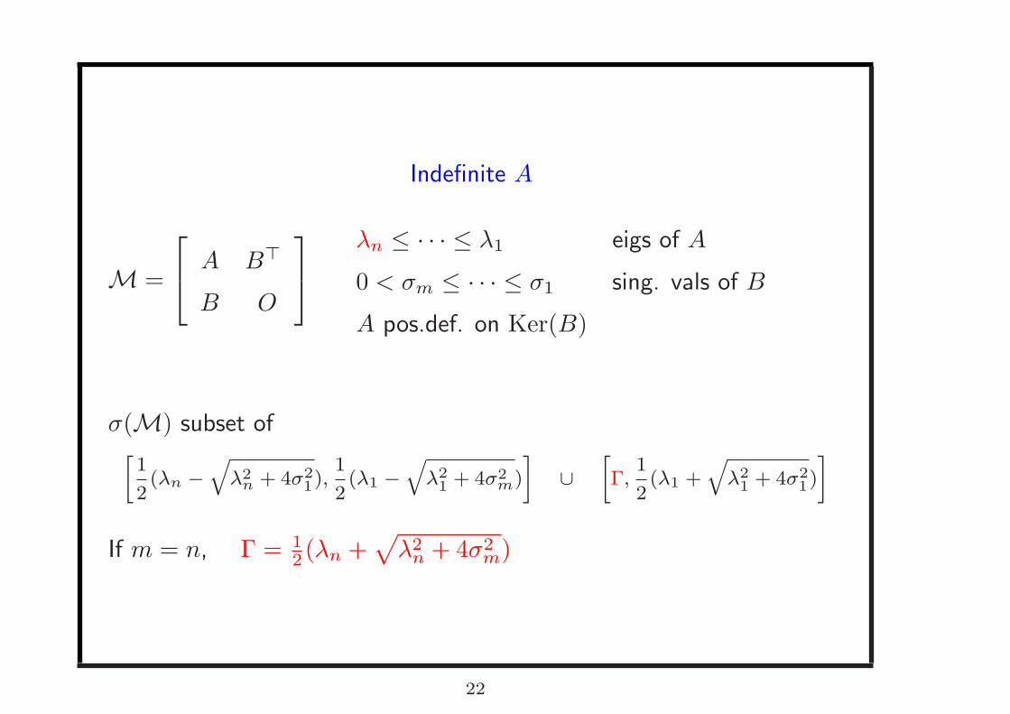
Application to ideal block diagonal preconditioners

Indefinite preconditioner, C = 0:

1. Let P+ = blkdiag(A, BA−1B⊤). Then

µ(P−1+ M) ⊂

{1,

1

2(1 +

√5),

1

2(1 −

√5)

}⊂ R;

2. Let P− = blkdiag(A,−BA−1B⊤). Then

µ(P−1− M) ⊂

{1,

1

2(1 + i

√3),

1

2(1 − i

√3)

}⊂ C

+.

34

Application to practical block diagonal preconditioners

Indefinite preconditioner, C = 0:

Let P± = blkdiag(A,±S) with A, S nonsingular. Then

µ(P−1± M) ⊂

{1,

1

2(1 +

√1 + 4ξ),

1

2(1 −

√1 + 4ξ)

}⊂ C,

ξ : (possibly complex) eigenvalues of (BA−1B⊤,±S)

35


Indefinite preconditioner, C 6= 0:

Let P+ = blkdiag(A, C + BA−1B⊤). Then

µ(P−1+ M) ⊂

{1,

1

2(1 ±

√5),

1

2θ(θ − 1 ±

√(1 − θ)2 + 4θ2)

}⊂ R.

θ finite eigs of (C + BA−1B⊤, C)

Similar results for P− = blkdiag(A,−C − BA−1B⊤)

36


Definite preconditioner, C = 0:

P(τ) =

PA

PC

,

PA ≈ PA(τ) = A + τB⊤B

PC ≈ PC(τ) = B(A + τB⊤B)−1B⊤

• Definite preconditioner on definite problem:

P(τ)−1M(τ) has eigenvalues

1, 1

2(1 +

√5), 1

2(1 −

√5)

with multiplicity n − m, m and m, respectively.

37

General nonsymmetric problem

M =

F B⊤

B −βC

F nonsymmetric

Preconditioning strategies (other alternatives are possible):

Ptr =

F B

±C

Pd =

F

±C

with C > 0

• F ≈ F

• F ≈ F + B⊤C−1B (augmentation block precond.)

For +C: P−1M indefinite

38

Augmentation block preconditioning

⋆ Appealing for F singular

For +C:

P−1

d M, P−1tr M have clusters in C

− and C+

⇒ Indefinite matrix ⇒ Elman’s bound not applicable

Analysis of clusters:

- Schotzau & Greif ’06 (F sym)

- Cao ’07

39

Nonstagnation condition revisited. Grcar tech.rep’89

Let φk be polynomial with φk(0) = 0. If 1

2(φk(M) + φk(M)⊤) > 0

then

‖rk‖ ≤(

1 − θ2min

‖φk(M)‖2

) 1

2


2(φk(M) + φk(M)⊤))

Elman’s bound: k = 1

The simplest case: k = 2

If φ2(H) > 0, then φ2(M) > 0 iff ‖Sφ2(H)−1/2‖ < 1

⇒ In Simoncini & Szyld ’08: φ2(λ) = λ2

⇒ Here: φ2(λ) = λ(λ − α), α = max{0, λ+(H) + λ−(H)}(λ+(H), λ−(H): closest pos/neg eigs to zero)

40



2(φk(M) + φk(M)⊤) > 0

then

‖rk‖ ≤(

1 − θ2min

‖φk(M)‖2

) 1

2


2(φk(M) + φk(M)⊤))






41



2(φk(M) + φk(M)⊤) > 0

then

‖rk‖ ≤(

1 − θ2min

‖φk(M)‖2

) 1

2


2(φk(M) + φk(M)⊤))






42

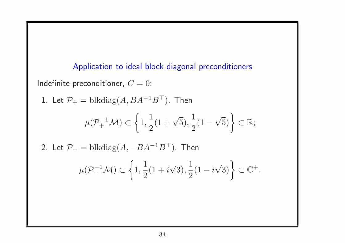
Example. Navier-Stokes problem

IFISS Package (Elman, Ramage, Silvester)

“Flow over a step”. Uniform grid, Q1-P0 elements

Prec blocks λmin(H) λmax(S⊤S, φ2(H)) α # its

Pd,augeC(0) -3.5512 0.9906 0.3951 16

eC(10−1) -2.7567 0.9724 0.4252 19

Q -4.2339 1.5620 0.3558 29

Ptr,augeC(0) -3.8091 0.9672 0 14

eC(10−1) -3.0814 1.1063 0.0216 21

eC(10−2) -3.7450 0.97097 0 16

PtrbF , W (1) -7.3000 0.9923 0 11

bF , W (0) -13.818 0.9924 0 17

eC(tol) = B eF−1B⊤ + βC eF = luinc(F, tol)

(2,2) block: W (s1) = B bF−1B⊤ + s1βC bF = luinc(F, 10−2)

43

Example. Navier-Stokes problem

IFISS Package (Elman, Ramage, Silvester)

“Flow over a step”. Uniform grid, Q1-P0 elements

Prec blocks λmin(H) λmax(S⊤S, φ2(H)) α # its

Pd,augeC(0) -3.5512 0.9906 0.3951 16

eC(10−1) -2.7567 0.9724 0.4252 19

Q -4.2339 1.5620 0.3558 29

Ptr,augeC(0) -3.8091 0.9672 0 14

eC(10−1) -3.0814 1.1063 0.0216 21

eC(10−2) -3.7450 0.97097 0 16

PtrbF , W (1) -7.3000 0.9923 0 11

bF , W (0) -13.818 0.9924 0 17

eC(tol) = B eF−1B⊤ + βC eF = luinc(F, tol)

(2,2) block: W (s1) = B bF−1B⊤ + s1βC bF = luinc(F, 10−2)

44

Spectrum of MP−1tr,aug

−1 −0.5 0 0.5 1 1.5−0.02

−0.015

−0.01

−0.005

0

0.005

0.01

0.015

0.02

real part

ima

gin

ary

pa

rt

45

GMRES Convergence history

0 2 4 6 8 10 12 14 1610

−10

10−8

10−6

10−4

10−2

100

number of iterations

no

rm o

f re

sid

ua

l

46

Mesh independence

Ptr,aug. (2,2) block: C = βC + BF−1B⊤,

n m λmin(H) λmax(S⊤S, φ2(H)) α # its

418 176 -3.8091 0.9672 0 14

1538 704 -3.7057 0.9662 0 15

5890 2816 -3.6710 0.9660 0 13

47

Final considerations and outlook

Symmetric case:

• Sharp bounds obtained for symmetric indefinite (1,1) block

• Future work: exploit this knowledge to devise and analyze effective

preconditioners

Nonsymmetric case:

• First attempt to provide convergence information on indefinite

problem

• Future work: devise more complete convergence analysis

48

Final considerations and outlook

Symmetric case:

• Sharp bounds obtained for symmetric indefinite (1,1) block

• Future work: exploit this knowledge to devise and analyze effective

preconditioners

Nonsymmetric case:

• First attempt to provide convergence information on indefinite

problem

• Future work: devise more complete convergence analysis

49

References

1. V. S. and Daniel B. Szyld , New conditions for non-stagnation of

minimal residual methods. Numerische Mathematik, v. 109, n.3

(2008), pp. 477-487.

2. Nick Gould and V. S., Spectral Analysis of saddle point matrices

with indefinite leading blocks. August 2008, To appear in SIAM J.

Matrix Analysis Appl.

3. V.S., On the non-stagnation condition for GMRES and application

to saddle point matrices, In preparation.

50

Documents

V. Simoncini - Dipartimento di Matematicasimoncin/prec09.pdf · Spectral analysis of saddle point matrices with indeﬁnite leading blocks V. Simoncini Dipartimento di Matematica,