UvA-DARE (Digital Academic Repository) Arterial spin labeling … · CBLM Majoie . M Smits . AJ Nederveen. PlosOne 9; 2014. ... ASL perfusion MR has matured to I the point where it

UvA-DARE is a service provided by the library of the University of Amsterdam (http://dare.uva.nl)

UvA-DARE (Digital Academic Repository)

Arterial spin labeling perfusion MRI: Inter-vendor reproducibility and clinical applicability

Mutsaerts, H.J.M.M.

Link to publication

Citation for published version (APA):Mutsaerts, H. J. M. M. (2015). Arterial spin labeling perfusion MRI: Inter-vendor reproducibility and clinicalapplicability.

General rightsIt is not permitted to download or to forward/distribute the text or part of it without the consent of the author(s) and/or copyright holder(s),other than for strictly personal, individual use, unless the work is under an open content license (like Creative Commons).

Disclaimer/Complaints regulationsIf you believe that digital publication of certain material infringes any of your rights or (privacy) interests, please let the Library know, statingyour reasons. In case of a legitimate complaint, the Library will make the material inaccessible and/or remove it from the website. Please Askthe Library: https://uba.uva.nl/en/contact, or a letter to: Library of the University of Amsterdam, Secretariat, Singel 425, 1012 WP Amsterdam,The Netherlands. You will be contacted as soon as possible.

Download date: 09 Apr 2020

https://dare.uva.nl/personal/pure/en/publications/arterial-spin-labeling-perfusion-mri-intervendor-reproducibility-and-clinical-applicability(5aab0ebf-9650-4975-809e-0701cb88e9ba).html

2

Inter-vendor reproducibility of pseudo-continuous arterial spin labeling at 3 Tesla

HJMM Mutsaerts

RME Steketee

DFR Heijtel

JPA Kuijer

MJP van Osch

CBLM Majoie

M Smits

AJ Nederveen

PlosOne 9; 2014. In press

39

Inter-vendor reproducibility of PCASL at 3 T Chapter 2

Abstract

Purpose Prior to the implementation of arterial spin labeling (ASL) in clinical multi-center studies, it is

important to establish its status quo inter-vendor reproducibility. This study evaluates and compares the

intra- and inter-vendor reproducibility of pseudo-continuous ASL (pCASL) as clinically implemented by

GE and Philips.

Material and Methods 22 healthy volunteers were scanned twice on both a 3T GE and a 3T Philips

scanner. The main difference in implementation between the vendors was the readout module: spiral 3D

fast spin echo vs. 2D gradient-echo echo-planar imaging respectively. Mean and variation of cerebral

blood flow (CBF) were compared for the total gray matter (GM) and white matter (WM), and on a

voxel-level.

Results Whereas the mean GM CBF of both vendors was almost equal (p=1.0), the mean WM CBF was

significantly different (p<0.01). The inter-vendor GM variation did not differ from the intra-vendor GM

variation (p=0.3 and p=0.5 for GE and Philips respectively). Spatial inter-vendor CBF and variation

differences were observed in several GM regions and in the WM.

Conclusion These results show that total GM CBF-values can be exchanged between vendors. For the

inter-vendor comparison of GM regions or WM, these results encourage further standardization of ASL

implementation among vendors.

40


Introduction

Arterial spin labeling (ASL) is an emerging magnetic resonance imaging (MRI) perfusion modality that

enables non-invasive cerebral perfusion measurements. Since ASL is virtually harmless, not hampered by

the blood-brain barrier and enables absolute quantification of cerebral blood flow (CBF), it is an

attractive tool compared to other perfusion imaging modalities 1, 2. Through several methodological

advances, ASL perfusion MRI has matured to the point where it can provide high quality whole-brain

perfusion images in only a few minutes of scanning 3. Its reproducibility has been established and its

CBF-maps are comparable with imaging methods based on exogenous tracers 4-7. ASL is commercially

available on all major MRI systems and clinical applications are under rapid development. ASL-based

CBF measurements are of clinical value in a number of cerebral pathologies, such as brain tumors,

cerebrovascular pathology, epilepsy and neurodegeneration 8, 9. Therefore, the initiation of large-scale

multi-center ASL studies is a next step to extend our understanding of the pathophysiology of many

common disorders.

However, it is essential to first establish the inter-vendor reproducibility of ASL 10, 11. One main obstacle

that impedes multi-center studies, is that fundamental differences exist between ASL implementations of

different vendors. Each MRI vendor has implemented a different labeling-readout combination, which

may seriously hamper the comparison of multi-vendor ASL-data 12. Since each labeling and readout

strategy exhibits specific advantages and disadvantages, a substantial technical heterogeneity is

introduced 13. Therefore, it remains unclear to which degree ASL-based CBF-maps from centers with

scanners of different vendors are comparable. The aim of the current study is to assess and compare the

intra- and inter-vendor reproducibility of pseudo-continuous ASL (pCASL) CBF measurements as

currently clinically implemented by two major vendors: i.e. GE and Philips.

Materials and Methods Subject recruitment and study design

Twenty-two healthy volunteers (9 men, 13 women, mean age 22.6 ± 2.1 (SD) years) were included. In

addition to standard MRI exclusion criteria, subjects with history of brain or psychiatric disease or use of

medication - except for oral contraceptives - were excluded. No consumption of vasomotor substances

such as alcohol, cigarettes, coffee, licorice and tea was allowed on the scan days. On the day prior to the

examination, alcohol and nicotine consumption was restricted to three units and cigarettes respectively.

41


All subjects were scanned twice at two academic medical centers in the Netherlands: Erasmus MC ‒

University Medical Center Rotterdam (center 1) and Academic Medical Center Amsterdam (center 2).

The inter-session time interval was kept at 1-4 weeks. MRI experiments were performed on a 3T GE

scanner at center 1 (Discovery MR750, GE Healthcare, Milwaukee, WI, US) and on a 3T Philips scanner

at center 2 (Intera, Philips Healthcare, Best, the Netherlands), both equipped with an 8-channel head coil

(InVivo, Gainesville, FL, US). Foam padding inside the head coil was used to restrict head motion

during scanning 10. Subjects were awake and had their eyes closed during all ASL scans.

Ethics statement

All subjects provided written informed consent and the study was approved by the ethical review boards

of both centers.

Acquisition

Each scan session included a pCASL and 1 mm isotropic 3D T1-weighted scan for segmentation and

registration purposes. For the acquisition of a single time-point CBF-map, pCASL has become the

preferred labeling strategy because of its relatively high signal-to-noise ratio (SNR) and wide availability

across all platforms 3, 14. On both scanners we employed the clinically implemented pCASL protocols

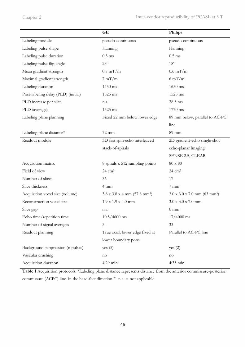
that are currently used in clinical studies 15, 16. Table 1 and Figure 1 summarize the protocol details and

show the timing diagrams for both sequences respectively. The main difference between the GE and

Philips implementations was the readout module: multi-shot spiral 3D fast spin-echo vs. single-shot 2D

gradient-echo echo-planar imaging respectively.

Post-processing: quantification

Matlab 7.12.0 (MathWorks, MA, USA) and Statistical Parametric Mapping (SPM) 8 (Wellcome Trust

Center for Neuroimaging, University College London, UK) were used for post-processing and statistical

analyses. For the Philips data, label and control pCASL images were pair-wise subtracted and averaged

to obtain perfusion-weighted images. For the GE data, the perfusion-weighted images as directly

provided by the scanner were used. Since the images as provided by GE did not incorporate motion

correction, this was not applied to the Philips data. The perfusion-weighted maps of both vendors were

quantified into CBF maps using a single compartment model 3, 17:

42


)1(2

6000min)/100/(1

1

/10

/

a

a

Taainv

TPLD

eTMMegmLCBF ταα −−

∆= [1]

where ΔM represents the difference images between control and label and M0a the equilibrium

magnetization of arterial blood. In Philips, ΔM was corrected for the transversal magnetization decay

time (T2*) of arterial blood (48 ms) during the 17 ms echo time (TE) by eTE/T2* 18. PLD is the post-

labeling delay (1.525 s), T1a is the longitudinal relaxation time of arterial blood (1.650 s), α is the labeling

efficiency (0.8), where α inv corrects for the decrease in labeling efficiency due to the 5 and 2 background

suppression pulses at GE (0.75) and Philips (0.83) respectively and τ represents the labeling duration

(1.450 s and 1.650 s for GE and Philips respectively) 19-21. The increase in label decay in the ascending

acquired 2D slices in Philips-data was accounted for. GE has, but Philips has not, implemented a

standard M0-acquisition where proton density maps are obtained with a saturation recovery acquisition

using readout parameters identical to the ASL readout. These maps were converted to M0a by the

following equation:

)1(

1

0

GM

satGM

a

Tte

PDM−

−=λ

[2]

where tsat is the saturation recovery time (2 s), T1GM is the relaxation time of gray matter (GM) tissue (1.2

s) and λGM is the GM brain-blood water partition coefficient (0.9 mL/g) 15, 22, 23. For the Philips data, a

single M0a-value was used for all subjects. This value was obtained in a previous study with the same

center, scanner, head coil, pCASL protocol and a similar population (n=16, 56% M, age 20-24 years) 24.

In short, cerebrospinal fluid T1 recovery curves were fitted on the control images of multiple time-point

pCASL measurements, with the same readout, without background suppression. The acquired M0 was

converted to M0a by multiplication with the blood water partition coefficient (0.76) and the density of

brain tissue (1.05 g/mL) 23, 25. No difference was made between the quantification of GM and WM CBF.

Post-processing: spatial normalization

A single 3D T1-weighted anatomical scan from each scanner for each subject (n=44) was segmented

into GM and white matter (WM) tissue probability maps. All CBF maps were transformed into

anatomical space by a rigid-body registration on the GM tissue probability maps. The tissue probability

maps were spatially normalized using the Diffeomorphic Anatomical Registration analysis using

Exponentiated Lie algebra (DARTEL) algorithm, and the resulting normalization fields were applied to

43


the CBF maps as well 26. Finally, all normalized images were spatially smoothed using an 8 x 8 x 8 mm

full-width-half-maximum Gaussian kernel, to minimize registration and interpolation errors.

Data analysis

All intra-vendor reproducibility analyses were based on a comparison of session 1 with session 2 within

each vendor (n=22). All inter-vendor reproducibility analyses were based on a comparison of GE

session 1 with Philips session 2, and GE session 2 with Philips session 1 (n=44). In this way, the

temporal physiological variation is expected to have an equal contribution to the intra- and inter-vendor

reproducibility. All reproducibility analyses were based on the mean CBF of the two sessions, and on the

mean and standard deviation of the paired inter-session CBF difference, denoted as ΔCBF and SDΔCBF

respectively. The within-subject coefficient of variation (wsCV) - a normalized parameter of variation -

was defined as the ratio of SDΔCBF to the mean CBF of both sessions:

meanCBF

SDwsCV CBF∆= %100 [3]

Reproducibility was assessed on a total GM and WM level, and on a voxel-level.

Data analysis: total supratentorial GM and WM

Mean CBF-values of each session were obtained for the total supratentorial GM and WM. GM and WM

masks were obtained by thresholding GM and WM probability maps at 70% and 95% tissue

probabilities respectively. GM-WM CBF ratios were calculated individually. The significance of paired

inter-session CBF differences (ΔCBF) was tested with a paired two-tailed Student's t-test. The Levene's

test was used to test the significance of the difference between GE SDΔCBF and Philips SDΔCBF, as well as

between the inter-vendor SDΔCBF and both intra-vendor SDΔCBF 27. Limits of agreement - defining the

range in which 95% of future measurements is expected to lie - were defined as ΔCBF ± 1.96 SDΔCBF 28.

Data analysis: voxel-level comparison

To assess spatial inter-vendor differences, CBF- and wsCV-values were computed for each voxel. For

CBF, both sessions and all subjects were averaged. To test significant voxel-wise inter-vendor CBF

differences, a Bonferroni-corrected paired two-tailed Student's t-test was performed (using both

sessions, n=44). Individual histograms of CBF (25 bins, range 0-160 mL/100g/min) were averaged to

generate a group-level histogram. A wsCV histogram (25 bins, range 5-45%) was generated from the

44


wsCV-maps. Both CBF and wsCV histograms were generated for the total supratentorial GM and WM

of each vendor. Statistical significance was set to p<0.05 for all tests.

45


GE Philips

Labeling module pseudo-continuous pseudo-continuous

Labeling pulse shape Hanning Hanning

Labeling pulse duration 0.5 ms 0.5 ms

Labeling pulse flip angle 23° 18°

Mean gradient strength 0.7 mT/m 0.6 mT/m

Maximal gradient strength 7 mT/m 6 mT/m

Labeling duration 1450 ms 1650 ms

Post-labeling delay (PLD) (initial) 1525 ms 1525 ms

PLD increase per slice n.a. 28.3 ms

PLD (average) 1525 ms 1770 ms

Labeling plane planning Fixed 22 mm below lower edge 89 mm below, parallel to AC-PC

line

Labeling plane distance* 72 mm 89 mm

Readout module 3D fast spin-echo interleaved

stack-of-spirals

2D gradient-echo single-shot

echo-planar imaging

SENSE 2.5, CLEAR

Acquisition matrix 8 spirals x 512 sampling points 80 x 80

Field of view 24 cm3 24 cm2

Number of slices 36 17

Slice thickness 4 mm 7 mm

Acquisition voxel size (volume) 3.8 x 3.8 x 4 mm (57.8 mm3) 3.0 x 3.0 x 7.0 mm (63 mm3)

Reconstruction voxel size 1.9 x 1.9 x 4.0 mm 3.0 x 3.0 x 7.0 mm

Slice gap n.a. 0 mm

Echo time/repetition time 10.5/4600 ms 17/4000 ms

Number of signal averages 3 33

Readout planning True axial, lower edge fixed at

lower boundary pons

Parallel to AC-PC line

Background suppression (n pulses) yes (5) yes (2)

Vascular crushing no no

Acquisition duration 4:29 min 4:33 min

Table 1 Acquisition protocols. *Labeling plane distance represents distance from the anterior commissure-posterior

commissure (ACPC) line in the head-feet direction 20. n.a. = not applicable

46


Figure 1. Sequence timing diagrams of a) General Electric (GE) and b) Philips, shown at the same time

scale (ms). pCASL = pseudo-continuous arterial spin labeling, PLD = post-labeling delay.

Results Session timing

The number of days between intra-vendor sessions did not differ between vendors: 18.3 ± 6.5 and 19.7

± 7.2 for GE and Philips respectively (independent sample Student's t-test, p=0.5). However, GE

session 1 and session 2 took place earlier in the day compared to the Philips sessions (15h26 ± 4h00 and

15h55 ± 3h34 compared to 20h16 ± 2h06 and 19h47 ± 2h38 respectively, p<0.01).

Total GM and WM

The intra- and inter-vendor statistics are summarized in Table 2 and visualized by the Bland-Altman

plots in Figure 2. GM CBF did not differ significantly between both vendors (p=1.0), but WM CBF did

(p<0.01). Likewise, the intra-vendor GM variances of the paired CBF differences did not differ between

the two vendors whereas the WM variances did (p=0.6 and p=0.02 respectively). The GM-WM CBF

ratios of both vendors differed significantly, the 2D readout (Philips) GM-WM ratio being

approximately twice as large as the ratio of the 3D readout (GE) (p<0.01). Both the GM and WM intra-

vendor wsCVs were similar to the inter-vendor wsCVs (Table 2), which is confirmed by the Levene's

47


test. The variance of GM inter-vendor CBF differences did not differ significantly from the variance of

intra-vendor differences (p=0.3 and p=0.5 for GE and Philips respectively). For the WM, however, the

variance of inter-vendor CBF differences did differ significantly from the Philips variance but not from

the GE variance (p=0.02 and p=0.8 respectively).

Table 2 Inter-session statistics. Mean and ΔCBF represent the inter-session CBF mean and paired

difference respectively. The limits of agreement (LOA) represent ΔCBF ± 1.96 standard deviation of the

paired difference (SDΔCBF). CI = confidence interval, CBF = cerebral blood flow, GE = General

Electric, GM = gray matter, WM = white matter, wsCV = within-subject coefficient of variation.

GE

CI

(n=22)

Philips

CI

(n=22)

inter-

vendor

CI

(n=44)

GM mean CBF (mL/100g/min) 65.9 48.4 ·· 83.4 65.9 42.0 ·· 89.8 65.9 45.4 ·· 86.4

GM ΔCBF - 0.4 -3.5 ·· 2.8 3.9 0.6 ·· 7.2 0.0 -2.7 ·· 2.7

GM SDΔCBF 7.1 4.8 ·· 9.4 7.5 5.1 ·· 9.8 8.9 7.0 ·· 10.9

GM lower LOA -14.3 -18.2 ·· -10.4 -10.7 -14.8 ·· -6.6 -17.5 -20.9 ·· -14.2

GM upper LOA 13.6 9.7 ·· 17.5 18.5 14.4 ·· 22.6 17.5 14.2 ·· 20.9

GM wsCV (%) 10.8 6.2 ·· 15.3 11.3 5.4 ·· 17.2 13.6 9.8 ·· 17.3

WM mean CBF (mL/100g/min) 30.5 22.0 ·· 39.0 15.4 9.1 ·· 21.7 22.9 15.6 ·· 30.3

WM ΔCBF -0.6 -2.2 ·· 1.0 1.0 0.1 ·· 2.0 15.0 14.0 ·· 16.1

WM SDΔCBF 3.6 2.4 ·· 4.7 2.1 1.4 ·· 2.8 3.5 2.7 ·· 4.2

WM lower LOA -7.6 -9.6 ·· -5.7 -3.1 -4.3 ·· -2.0 8.3 7.0 ·· 9.6

WM upper LOA 6.4 4.4 ·· 8.3 5.2 4.1 ·· 6.4 21.8 20.5 ·· 23.1

WM wsCV (%) 11.7 9.5 ·· 13.9 13.8 12.2 ·· 15.4 15.0 13.7 ·· 16.4

GM-WM CBF ratio 2.2 1.9 ·· 2.5 4.3 3.4 ·· 5.2 2.9 2.4 ·· 3.4

48


Figure 2. Bland-Altman plots. Intra-vendor a) GE (n=22) and b) Philips (n=22) and c) inter-vendor

(n=44) GM (red) and WM (blue) CBF differences are plotted against mean CBF. Continuous and

broken lines indicate mean difference and limits of agreement (mean difference ± 1.96 standard

deviation of the paired difference) respectively. CBF= cerebral blood flow, GM=gray matter,

WM=white matter.

Voxel-level comparison Spatial CBF differences between GE and Philips are illustrated for a single subject and on group level in

Figure 3 and 4 respectively. The spatial wsCV distribution is shown in Figure 5. In addition, Figure 6

provides an overview of spatial CBF differences between subjects, sessions and vendors for a single

transversal slice. The main visual difference on all these maps was the homogeneity of GE compared to

the heterogeneity of Philips, especially in the WM and in the z-direction. More specifically, the contrast

between GM and WM was higher on the Philips CBF and wsCV-maps. Also within the GM, the CBF

was more heterogeneous on the Philips maps compared to the GE maps. A CBF decrease and wsCV

increase was observed in the posterior and superior regions on the GE maps and in the anterior-inferior

and superior regions on the Philips maps. The GM CBF histograms were comparable between vendors

(Figure 4d). The GE WM CBF histogram had a higher mean, but had the same shape as the Philips WM

CBF histogram. The wsCV histograms, on the other hand, were less comparable (Figure 5d). The spatial

GM wsCV distribution of Philips had a higher mean and was wider compared to GE. This difference in

mean and spread was even larger for the WM.

49


Figure 3. Cerebral blood flow maps of a representative subject of GE (b) and Philips (c), as compared

to gray matter (GM) tissue probability map (a; for this example the GE 3D T1-weighted image was

used). Maps are registered, re-sliced, skull-stripped and shown in native space.

50


Figure 4. Mean cerebral blood flow (CBF) maps of all subjects (n=22) are shown for GE (a) and Philips (b), averaged for both sessions. Voxel-wise

significant inter-vendor differences are visualized by a binary parametric map projected on the gray matter (GM) probability map (c). Red voxels

represent where GE < Philips, blue voxels represent where GE > Philips (Bonferroni corrected p<0.05). On the right, mean CBF histograms are

shown for the total GM and white matter (WM) (d).

51


Figure 5. a) GE and b) Philips intra- and c) inter-vendor within-subject coefficient of variability (wsCV)-maps. d) wsCV histograms are shown on the

right for the total gray matter (GM) and white matter (WM).

52


Figure 6. Single transversal cerebral blood flow slice of all subjects (n=22) for GE (upper quadrants)

and Philips (lower quadrants), session 1 (left quadrants) and session 2 (right quadrants), after spatial

normalization.

Discussion The most important result of this study is that - despite several voxel-wise differences between vendors -

there were no inter-vendor differences in mean CBF or wsCV on a total GM level. This can be

explained by the fact that the variation between the sessions can for a large part be attributed to

physiological factors, as was previously noted in single-vendor reproducibility studies 11, 29-31. For clinical

studies that focus on the GM in total, it may therefore be more important to minimize and account for

physiological variation than to account for inter-vendor differences in ASL implementation.

A different picture arises for smaller GM regions or for the total WM. We observed several spatial

differences between vendors which can mainly be explained by differences in the readout module. The

most visually striking inter-vendor difference on all CBF- and wsCV-maps was in the WM. The GM-

53


WM CBF ratio of the 2D readout (Philips) was twice as large as the ratio of the 3D readout (GE), which

is in agreement with a previous readout comparison on a single Siemens scanner 13. This can be

explained by the larger extent of spatial smoothing of a spiral 3D readout (GE) compared to the 2D

readout (Philips), which leads to more contamination of the GM signal into the WM and vice versa.

Therefore, a 2D readout seems most suitable when the goal is to acquire uncontaminated GM or WM

CBF ‒ although the ability of ASL to measure WM CBF is debatable due to the long transit time of WM 32.

This difference in spatial smoothing may also explain the homogeneous GM appearance of the mean

CBF and wsCV maps acquired with GE as compared to the more heterogeneous appearance of those

acquired with Philips. In addition, it may explain the significant inter-vendor CBF difference within the

subcortical GM since this area is surrounded by WM and therefore suffers more from smoothing with

WM signal in GE (Figure 4c). Another explanation for the smaller spatial variation of GE, is its higher

SNR compared to Philips. The SNR at GE is most probably higher because of the intrinsically high

SNR of a 3D readout and because background suppression is more efficient for a single-volume readout

as compared to a multi-slice readout 13. In addition, parallel imaging was not available in the GE

sequence, but was turned on in the Philips sequence. To what extent the heterogeneous appearance of

the Philips CBF maps has a physiological origin or is rather the result of a too low SNR, cannot be

differentiated with these data.

In regions with long arrival times - i.e. the posterior vascular territory and posterior watershed area -

lower CBF and higher wsCV was observed in GE but not in Philips (Figures 4 and 5) 5. This inter-

vendor difference can be explained by differences in the effective post-labeling delay (PLD) between the

readouts, even though both acquisitions had the same initial PLD (1525 ms). Whereas the 3D readout

obtains all ASL signal for the total 3D volume at a single time-point - i.e. after 1525 ms PLD - the 2D

readout obtains signal from each slice sequentially. With this multi-slice acquisition, each slice exhibits a

longer effective PLD compared to its previous slice. This inferior-superior PLD increase of the 2D

readout (Philips) allows the labeled blood more time to reach the superior slices compared to the

homogeneous PLD of the 3D readout (GE). Therefore, the PLD may have been too short for the label

to reach the superior slices in 3D (GE), whereas the effective PLD for the superior slices in 2D (Philips)

was sufficient. These inter-vendor CBF differences and higher wsCV for GE in superior regions with

long transit times are probably resolved by selecting a longer PLD for the 3D readout, such as 2000 ms 3.

54


Other prominent spatial inter-vendor CBF (Figure 4) and wsCV (Figure 5) differences were observed on

the brain edges. We observed higher CBF and lower wsCV in anterior and inferior regions in Philips but

not in GE. The prominent inferior CBF and wsCV differences (Figure 4c and Figure 5c) are partly due

to the fact that these slices were simply not acquired by the 2D readout (Philips). With a 2D sequence, it

is common practice to scan cerebral slices only as well as to optimize the PLD, T1 decay and

background suppression for the cerebral slices. These issues do not apply for a 3D sequence, whose 3D

slab usually has whole-brain coverage. The differences in the other areas can be explained by

susceptibility artifacts from bone-air transitions at the paranasal sinuses and mastoid air cells present in

the gradient-echo T2*-weighted readout implemented by Philips 33. In addition, it is expected that the

echo-planar imaging readout (Philips) exhibits geometric distortion in these regions 33. The T2-weighted

spin-echo readout employed by GE is much less sensitive to these artifacts, in comparison to the

gradient-echo readout employed by Philips. For these reasons, a 3D readout is superior in regions such

as the orbito-frontal lobe and cerebellum compared to a 2D readout. This especially favors the use of a

3D readout for clinical applications of ASL, since pathologies in these regions could remain undetected

on a 2D readout 34-36.

A limitation of the current study is that we did not acquire spatial M0-maps with the same readout in

Philips. By employing a voxel-wise normalization of the ASL-signal, these maps would have opposed the

T2* susceptibility effects, since these will be approximately equally large for the ΔM and M0-map.

Therefore, Philips spatial M0a-maps could have improved quantification in regions of air-tissue

transitions, which may have diminished the inter-vendor variation to a certain extent. However, the

added value of spatial M0-maps is limited since they cannot improve the lower SNR of the gradient-echo

readout (Philips) near the air-tissue transitions. Therefore, the inter-vendor reproducibility in these

regions is expected to remain low.

The current study may also be limited by the inter-vendor calibration of quantification parameters. These

may remain arbitrary, mostly because they have been derived from simulations rather than

measurements. One example is the inter-vendor differences in labeling efficiency due to a different

number of background suppression pulses (5 and 2 for GE and Philips respectively) 21. One way to deal

with this is to scale to a phase-contrast MRI sequence of the main feeding arteries 20. However, this

would shift the inter-vendor CBF variation from the ASL-sequence towards the phase-contrast MRI

measurements.

55


Inter-vendor CBF and wsCV differences were observed on a voxel-level but not on the total GM level.

Apparently, the effects of the abovementioned readout differences do cancel out when sufficient GM

voxels are averaged. There are several explanations for this observation. First, the higher SNR of the 3D

module may be important on a voxel-level, but if sufficient GM voxels are averaged physiological

variation seems to outnumber the SNR differences between the readout modules. Second, the

smoothing of the GE 3D readout averages signal from multiple GM voxels which increases SNR and

subsequently decreases the wsCV within a single voxel. This effect is similar to averaging signal from

multiple GM voxels of the 2D readout in post-processing. Therefore, this difference of spatial signal

averaging between both readouts becomes apparent on a voxel-level but is negligible when all GM

voxels are averaged.

It should be acknowledged that this study evaluated healthy controls only. The abovementioned inter-

vendor readout differences could become more or less important in patients, considering the different

spatial CBF variation in patients compared to healthy controls. Furthermore, these inter-vendor

differences should not be generalized to all MRI vendors. Visual readout differences between GE and

Siemens, who both use a 3D approach, may be smaller than the readout differences in the current study 13.

In conclusion, the current study shows that pCASL results do not differ between vendors on a total GM

level. Therefore, the reliability of averaged CBF-values for the total GM can be expected to be equal in

single- and multi-vendor studies. However, the reliability of measurements in GM regions or in the WM,

is impeded by differences between the readout modules of both vendors. Therefore, our results strongly

encourage the standardization of ASL implementations among vendors, which was also advocated by

the recent ASL consensus paper 3.

56


Reference list

1. Golay X, Hendrikse J, Lim TC. Perfusion imaging using arterial spin labeling. Top Magn Reson Imaging 2004; 15(1):10-27.

2. Williams DS, Detre JA, Leigh JS, Koretsky AP. Magnetic resonance imaging of perfusion using spin inversion of arterial water. Proc Natl Acad Sci U S A 1992; 89(1):212-216.

3. Alsop DC, Detre JA, Golay X, Gunther M, Hendrikse J, Hernandez-Garcia L, et al. Recommended implementation of arterial spin-labeled perfusion MRI for clinical applications: A consensus of the ISMRM perfusion study group and the European consortium for ASL in dementia. Magn Reson Med 2014.

4. Chen Y, Wolk DA, Reddin JS, Korczykowski M, Martinez PM, Musiek ES, et al. Voxel-level comparison of arterial spin-labeled perfusion MRI and FDG-PET in Alzheimer disease. Neurology 2011; 77(22):1977-1985.

5. Petersen ET, Mouridsen K, Golay X. The QUASAR reproducibility study, Part II: Results from a multi-center Arterial Spin Labeling test-retest study. Neuroimage 2010; 49(1):104-113.

6. Xu G, Rowley HA, Wu G, Alsop DC, Shankaranarayanan A, Dowling M, et al. Reliability and precision of pseudo-continuous arterial spin labeling perfusion MRI on 3.0 T and comparison with 15O-water PET in elderly subjects at risk for Alzheimer's disease. NMR Biomed 2010; 23(3):286-293.

7. Jahng GH, Song E, Zhu XP, Matson GB, Weiner MW, Schuff N. Human brain: reliability and reproducibility of pulsed arterial spin-labeling perfusion MR imaging. Radiology 2005; 234(3):909-916.

8. Detre JA, Rao H, Wang DJ, Chen YF, Wang Z. Applications of arterial spin labeled MRI in the brain. J Magn Reson Imaging 2012; 35(5):1026-1037.

9. Hendrikse J, Petersen ET, Golay X. Vascular disorders: insights from arterial spin labeling. Neuroimaging Clin N Am 2012; 22(2):259-2xi.

10. Golay X. How to do an ASL multicenter neuroimaging study. In: International Society of Magnetic Resonance in Medicine; 2009.

11. Liu T, Wierenga C, Mueller B, F-BIRN. Reliability and Reproducibility of Arterial Spin Labeling Perfusion Measures Assessed with a Multi-Center Study. In: International Society of Magnetic Resonance in Medicine; 2008. p. 3338.

12. Kilroy E, Apostolova L, Liu C, Yan L, Ringman J, Wang DJ. Reliability of two-dimensional and three-dimensional pseudo-continuous arterial spin labeling perfusion MRI in elderly populations: Comparison with 15o-water positron emission tomography. J Magn Reson Imaging 2013.

13. Vidorreta M, Wang Z, Rodriguez I, Pastor MA, Detre JA, Fernandez-Seara MA. Comparison of 2D and 3D single-shot ASL perfusion fMRI sequences. Neuroimage 2012; 66C:662-671.

14. Chen Y, Wang DJ, Detre JA. Test-retest reliability of arterial spin labeling with common labeling strategies. J Magn Reson Imaging 2011; 33(4):940-949.

15. Binnewijzend MA, Kuijer JP, Benedictus MR, van der Flier WM, Wink AM, Wattjes MP, et al. Cerebral blood flow measured with 3D pseudocontinuous arterial spin-labeling MR imaging in Alzheimer disease and mild cognitive impairment: a marker for disease severity. Radiology 2013; 267(1):221-230.

16. Donahue MJ, Ayad M, Moore R, van OM, Singer R, Clemmons P, et al. Relationships between hypercarbic reactivity, cerebral blood flow, and arterial circulation times in patients with moyamoya disease. J Magn Reson Imaging 2013.

17. Alsop DC, Detre JA. Reduced transit-time sensitivity in noninvasive magnetic resonance imaging of human cerebral blood flow. J Cereb Blood Flow Metab 1996; 16(6):1236-1249.

18. St Lawrence KS, Wang J. Effects of the apparent transverse relaxation time on cerebral blood flow measurements obtained by arterial spin labeling. Magn Reson Med 2005; 53(2):425-433.

57


19. Lu H, Clingman C, Golay X, van Zijl PC. Determining the longitudinal relaxation time (T1) of blood at 3.0 Tesla. Magn Reson Med 2004; 52(3):679-682.

20. Aslan S, Xu F, Wang PL, Uh J, Yezhuvath US, van OM, et al. Estimation of labeling efficiency in pseudocontinuous arterial spin labeling. Magn Reson Med 2010; 63(3):765-771.

21. Garcia DM, Duhamel G, Alsop DC. Efficiency of inversion pulses for background suppressed arterial spin labeling. Magn Reson Med 2005; 54(2):366-372.

22. Lu H, Nagae-Poetscher LM, Golay X, Lin D, Pomper M, van Zijl PC. Routine clinical brain MRI sequences for use at 3.0 Tesla. J Magn Reson Imaging 2005; 22(1):13-22.

23. Herscovitch P, Raichle ME. What is the correct value for the brain--blood partition coefficient for water? J Cereb Blood Flow Metab 1985; 5(1):65-69.

24. Heijtel DF, Mutsaerts HJ, Bakker E, Schober P, Stevens MF, Petersen ET, et al. Accuracy and precision of pseudo-continuous arterial spin labeling perfusion during baseline and hypercapnia: a head-to-head comparison with O HO positron emission tomography. Neuroimage 2014.

25. Chalela JA, Alsop DC, Gonzalez-Atavales JB, Maldjian JA, Kasner SE, Detre JA. Magnetic resonance perfusion imaging in acute ischemic stroke using continuous arterial spin labeling. Stroke 2000; 31(3):680-687.

26. Ashburner J. A fast diffeomorphic image registration algorithm. Neuroimage 2007; 38(1):95-113. 27. levene, howard, Olkin I, Hotelling H. Contributions to Probability and Statistics: Essays in Honor of

Harold Hotelling: Stanford University Press; 1960. 28. Bland JM, Altman DG. Measuring agreement in method comparison studies. Stat Methods Med Res

1999; 8(2):135-160. 29. Floyd TF, Ratcliffe SJ, Wang J, Resch B, Detre JA. Precision of the CASL-perfusion MRI

technique for the measurement of cerebral blood flow in whole brain and vascular territories. J Magn Reson Imaging 2003; 18(6):649-655.

30. Parkes LM, Rashid W, Chard DT, Tofts PS. Normal cerebral perfusion measurements using arterial spin labeling: reproducibility, stability, and age and gender effects. Magn Reson Med 2004; 51(4):736-743.

31. Gevers S, van Osch MJ, Bokkers RP, Kies DA, Teeuwisse WM, Majoie CB, et al. Intra- and multicenter reproducibility of pulsed, continuous and pseudo-continuous arterial spin labeling methods for measuring cerebral perfusion. J Cereb Blood Flow Metab 2011; 31(8):1706-1715.

32. van Gelderen P, de Zwart JA, Duyn JH. Pittfalls of MRI measurement of white matter perfusion based on arterial spin labeling. Magn Reson Med 2008; 59(4):788-795.

33. Deichmann R, Josephs O, Hutton C, Corfield DR, Turner R. Compensation of susceptibility-induced BOLD sensitivity losses in echo-planar fMRI imaging. Neuroimage 2002; 15(1):120-135.

34. Timmann D, Konczak J, Ilg W, Donchin O, Hermsdorfer J, Gizewski ER, et al. Current advances in lesion-symptom mapping of the human cerebellum. Neuroscience 2009; 162(3):836-851.

35. Wolf RC, Thomann PA, Sambataro F, Vasic N, Schmid M, Wolf ND. Orbitofrontal cortex and impulsivity in borderline personality disorder: an MRI study of baseline brain perfusion. Eur Arch Psychiatry Clin Neurosci 2012; 262(8):677-685.

36. Walther S, Federspiel A, Horn H, Razavi N, Wiest R, Dierks T, et al. Resting state cerebral blood flow and objective motor activity reveal basal ganglia dysfunction in schizophrenia. Psychiatry Res 2011; 192(2):117-124.

58

Documents

UvA-DARE (Digital Academic Repository) Arterial spin labeling … · CBLM Majoie . M Smits . AJ Nederveen. PlosOne 9; 2014. ... ASL perfusion MR has matured to I the point where it