Accepted Manuscript

Utilizing correlated node mobility for efficient DTN routing

Eyuphan Bulut, Sahin Cem Geyik, Boleslaw K. Szymanski

PII: S1574-1192(13)00120-XDOI: http://dx.doi.org/10.1016/j.pmcj.2013.09.007Reference: PMCJ 446

To appear in: Pervasive and Mobile Computing

Received date: 28 November 2012Revised date: 14 September 2013Accepted date: 20 September 2013

Please cite this article as: E. Bulut, S.C. Geyik, B.K. Szymanski, Utilizing correlated nodemobility for efficient DTN routing, Pervasive and Mobile Computing (2013),http://dx.doi.org/10.1016/j.pmcj.2013.09.007

This is a PDF file of an unedited manuscript that has been accepted for publication. As aservice to our customers we are providing this early version of the manuscript. The manuscriptwill undergo copyediting, typesetting, and review of the resulting proof before it is published inits final form. Please note that during the production process errors may be discovered whichcould affect the content, and all legal disclaimers that apply to the journal pertain.

Utilizing Correlated Node Mobility for Efficient DTN

Routing

Eyuphan Buluta,b, Sahin Cem Geyika, Boleslaw K Szymanskia,c

aRensselaer Polytechnic Institute, 110 8th St, Troy, NY 12180Email:{bulute,geyiks, szymansk}@cs.rpi.edu

b2200 President George Bush Highway, Richardson, TX 75082Email:ebulut@cisco.com

cSpo leczna Akademia Nauk ul Sienkiewicza 9, 90-113 Lodz, Poland

Abstract

In a delay tolerant network (DTN), nodes are connected intermittently andthe future node connections are mostly not known. Therefore, effective for-warding based on limited knowledge of contact behavior of nodes is chal-lenging. Most of the previous studies assumed that mobility of a node isindependent from mobility of other nodes and looked at only the pairwisenode relations to decide routing. In contrast, in this paper, we analyze thetemporal correlation between the meetings of each node with other nodesand utilize this correlation for efficient routing. We introduce a new metriccalled conditional intermeeting time (CIT), which computes the average in-termeeting time between two nodes relative to a meeting with a third node.Then, we modify existing DTN routing protocols using the proposed metricto improve their performance. Extensive simulations based on real and syn-thetic DTN traces show that the modified algorithms perform better thanthe original ones.

Keywords: Delay Tolerant Networks, routing, efficiency, temporalcorrelation.

1. Introduction

Delay tolerant networks (DTN) are wireless networks in which at anygiven time instance, the probability that there is an end-to-end path froma source to a destination is low due to the high mobility and low densityof the nodes in the network. Routing of messages in such a challenging

Preprint submitted to Pervasive and Mobile Computing September 14, 2013

*ManuscriptClick here to view linked References

DTN environment is achieved opportunistically by utilizing store-carry-and-forward paradigm at each node. Several DTN routing algorithms based onthis paradigm have been proposed recently. In each, different techniques(single-copy [1]-[5], multi-copy [6]-[8], erasure coding [9] [10]) with slightlydifferent goals have been utilized. A survey of DTN routing algorithms canbe found in [11].

Since DTNs consist of mobile agents that contact intermittently, recentstudies on DTN routing have focused on the analysis of real mobility traces(human [12], vehicular [13] etc.) and utilized extracted characteristics of themobile objects in the design of forwarding algorithms for DTNs.

Reviewing these designs and analyses, we have made the following ob-servations. First, the future meetings of nodes can be predicted from theirpast relations using some distribution functions (e.g. log-normal [14] [15]).Second, most of the previous routing protocols assume that meetings of anode with other nodes are independent from each other. Some algorithms(e.g. Bubblerap [19]) implicitly consider the dependency between the nodemeetings thanks to their designs which use real traces, however, there is noanalysis and explicit usage of temporal correlation between the meetings oftwo nodes with a third node. Third, the mobility of many real objects arenon-deterministic but periodic [22]. For example, in a cyclic MobiSpace, iftwo nodes were frequently in contact at a particular time in previous cycles,then they are likely to meet around the same time in the next cycle.

The above observations motivated us to study temporal correlation be-tween the node meetings for designing more efficient routing algorithms.Hence, we introduce a new link metric, conditional intermeeting time (CIT),that computes the average intermeeting time between two nodes relative toa meeting with a third node using only local knowledge of the past contacts.Note that this definition makes more sense in the context of routing becauseit refers to message holding time on a given node during message routing.

We analyze CIT and discuss when and why it is beneficial in providingaccurate information to nodes making routing decisions. Different than ourinitial work [37], we also present statistical results from four different datasets (RollerNet [15], Cambridge [28], Haggle [30], MIT [36]) which containthe contact traces of real objects logged during real life experiments.

We then propose modifications to the existing DTN routing protocols us-ing the proposed metric and demonstrate how their performance improvesas the result. First, for the algorithms which route messages over shortestpaths (SP) [23] [24], we propose to use CIT rather than standard intermeeting

2

times (SIT) and route the messages over conditional shortest paths (CSP).Second, for the algorithms which make message forwarding decisions depend-ing on a delivery metric (we call them metric-based forwarding algorithms),we propose to use CIT as a secondary delivery metric and allow the forward-ing of messages if and only if both the algorithm’s original delivery metricand CIT agree to forward the message to the encountered node. Throughsimulations, we show the benefit of proposed approach. In this extendedversion, we added new simulation results and comparisons over our initialwork [37]. In addition to real DTN traces, we also utilized synthetic andlarge-scale traces for simulations. Moreover, we added new results showingthe superiority of the proposed approach over other popular algorithms (i.e.,SimBet and CREST) and added new graphs showing the effects of some im-portant parameters (buffer space at nodes, message generation interval, andtotal node count) on the results.

The remaining of the paper is organized as follows. In Section 2, wedescribe the proposed metric (CIT) in detail and in Section 3, we provide itsanalysis. In Section 4, we describe how it can be used to modify existing DTNrouting algorithms for performance improvement. In Section 5, we presentsimulation results. Finally, we offer conclusions and outline the future workin Section 6.

2. Conditional Intermeeting Time

Recently, the research community working on routing algorithms in DTNshas focused on the analysis of real mobility traces to understand the maincharacteristics of mobile objects. Several experiments in different environ-ments (office [14], conference [30], city [28], skating tour [15]) with differentobjects (human [12], bus [13]) and with variable number of attendants wereperformed. From the analysis of the data sets collected during these exper-iments, significant results about the aggregate and pairwise mobility char-acteristics of real objects were obtained and different kinds of algorithmsusing different metrics developed for efficient routing of messages in DTNs.For example, in SimBet [18], a joint utility metric based on social similar-ity and egocentric betweenness of nodes is used. In BubbleRap [19] tworankings (global and local) is used to compute each node’s popularity (i.e.,connectivity) in the local community and entire society. Routing of mes-sages are then performed via nodes with high utility values. Moreover, inLocalCom [20], a community-based epidemic forwarding scheme, which first

3

4 time units/cycle3 time units/

2 time unitsM

A

B

cycle

cycle

Figure 1: An example cyclic MobiSpace with a common motion cycle of 12 time units.

detects the community structure of the network and forwards the messagesto each community through gateways, is proposed.

Even though the previous studies modeled the node relations (i.e., inter-meeting times) using different distributions (exponential [7] [31], log-normal [15])and developed their routing metrics accordingly, they assumed that the meet-ings of a node with other nodes is independent of each other. The futuremeetings of two nodes are predicted looking at the meetings of only thesetwo nodes in the past. In [14], one additional attribute (the time passed sincethe last meeting) is also taken into account for more accurate prediction.However, as we show with statistics from real DTN traces, the meetings of anode with other nodes may not be independent from each other (i.e., meet-ings are correlated), thus, prediction of future node relations can be furtherimproved with the analysis of temporal correlation between node meetings.In [5], each node establishes a community of nodes with whom it frequentlymeets to use for routing decisions when this node meets a message carrier.In contrast, in this paper, we consider a sequence of meetings of two specificnodes and use the statistics about subsequent meetings of those nodes withthe destination to make routing decisions.

We introduce a new metric called conditional intermeeting time (CIT) todefine the node relations more precisely within the context of routing. Thismetric computes the average intermeeting time between two nodes relativeto a meeting with an intermediate node using only the local knowledge ofthe past contacts.

The proposed metric can provide higher accuracy of prediction of deliverytime, especially if the nodes move in a cyclic MobiSpace [22]. Accordingto the definition of a cyclic MobiSpace, if two nodes contacted frequentlyat a particular time in previous cycles, the probability that they will be in

4

contact around the same time in the next cycle is high. In Figure 1, a samplecyclic MobiSpace with three objects is illustrated. The fully repeating motioncycle is 12 time units. In this example, the discrete probabilistic contactsbetween A and M happen every 12 time units (1, 13, 25 ...) and the discreteprobabilistic contacts between A and B occur every 6 time units (2, 8, 14...). When we consider the intermeeting time between nodes A and B, wecan expect that node A will forward its message to node B in 3 time units(since message can arrive at A at any time within 6 sec), however CIT of Awith B based on the condition that it has met (received the message from)node M lets us know that the message will be forwarded to node B within 1time unit.

Algorithm 1 updateSIT (node m, time t)

1: if m is seen first time then2: firstTimeAt[m] ← t3: else4: increment βm by 15: lastTimeAt[m] ← t6: end if7: for each neighbor i ∈ N do8: τs(i) ← (lastTimeAt[i] − firstTimeAt[i] ) / βi

9: end for

Each node in a DTN can compute its SIT and CIT with other nodes usingits contact history. In Algorithm 1, we show how a node, s, can compute thesemetrics from previous node meetings. The notations we use in this algorithm(and also throughout the paper) are listed below with their meanings:

• τA(B|M): Average time it takes for node A to meet node B aftermeeting with node M . If B=M , the notation (in short τA(B)) showsthe standard intermeeting time (SIT) between nodes A and B.

• S: NxN matrix where S(i, j) is the sum of all samples of conditionalintermeeting times with node j relative to the meeting with node i.Here, N is the neighbor count of current node (i.e., N(s) for node s).

• C: NxN matrix where C(i, j) is the number of all conditional inter-meeting time samples with node j relative to meeting with node i.

5

Algorithm 2 updateCIT (node m, time t)

1: for each neighbor j ∈ N and j 6= m do2: start a timer tmj

3: end for4: for each neighbor j ∈ N and j 6= m do5: for each timer tjm running do6: S[j][m] += time on tjm7: increment C[j][m] by 18: end for9: if S[j][m] 6= 0 then

10: τs(m|j) ← S[j][m] / C[j][m]11: end if12: delete all timers tjm13: end for

• βi: Total number of meetings with node i.

To find the CIT τA(B|M), each time node A meets node M , it starts adifferent timer for B. When it meets node B, it sums up the values of thesetimers before deleting them. The value of τA(B|M) is then calculated bydividing the current total of collected timer values by the number of timersused so far. In Algorithm 2, we explain this procedure. Note that whenthe node meets any node m, a timer is started for every other possible node(lines 1-3). Since meeting with node m will also end the conditional meetingtime process for some other nodes, the corresponding timers whose clock hasstarted at meeting with other nodes but is scheduled to end at meeting withm stop and their values are recorded (lines 4-8). CIT values are then updatedfor all possible cases and the timers are deleted (lines 9-12). We can also usea sliding window with an appropriate size over the past contacts [24] andtake into account the edge effects [13] to make the computation more localand current. Moreover, we do not consider the contact durations in thesecomputations since inter-contact times are usually much longer than contacttimes in real DTNs. However, if the last assumption does not hold, it is easyto modify all computations accordingly.

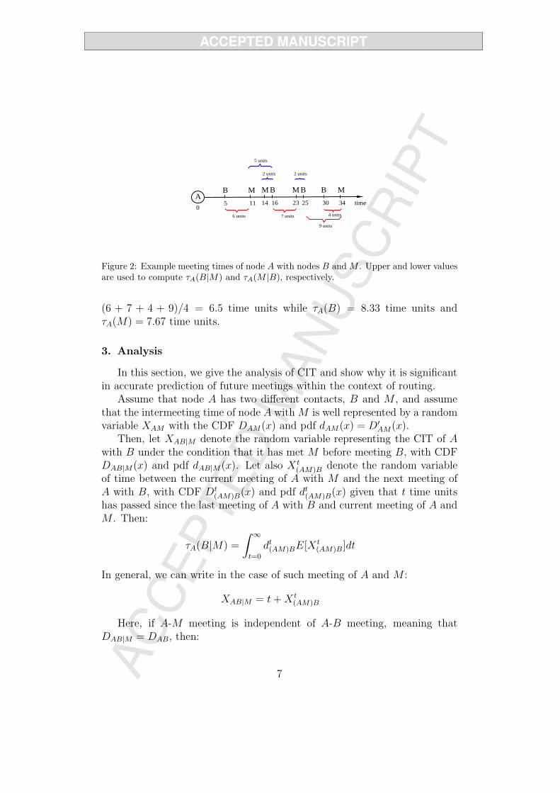
Consider the sample meeting times of a node A with its neighbors Band M in Figure 2. Node A meets with node B at times {5, 16, 25, 30} andwith node M at times {11, 14, 23, 34}. Following the procedure describedabove, we find that τA(B|M) = (5+2+2)/3 = 3 time units and τA(M |B) =

6

AB

5

M

11

M

14

B

16

M

23

B

25

B

30

M

34 time

6 units 7 units 4 units

9 units

5 units

2 units 2 units

0

Figure 2: Example meeting times of node A with nodes B and M . Upper and lower valuesare used to compute τA(B|M) and τA(M |B), respectively.

(6 + 7 + 4 + 9)/4 = 6.5 time units while τA(B) = 8.33 time units andτA(M) = 7.67 time units.

3. Analysis

In this section, we give the analysis of CIT and show why it is significantin accurate prediction of future meetings within the context of routing.

Assume that node A has two different contacts, B and M , and assumethat the intermeeting time of node A with M is well represented by a randomvariable XAM with the CDF DAM(x) and pdf dAM(x) = D′

AM(x).Then, let XAB|M denote the random variable representing the CIT of A

with B under the condition that it has met M before meeting B, with CDFDAB|M(x) and pdf dAB|M(x). Let also X t

(AM)B denote the random variableof time between the current meeting of A with M and the next meeting ofA with B, with CDF Dt

(AM)B(x) and pdf dt(AM)B(x) given that t time units

has passed since the last meeting of A with B and current meeting of A andM . Then:

τA(B|M) =

∫ ∞

t=0

dt(AM)BE[X t

(AM)B ]dt

In general, we can write in the case of such meeting of A and M :

XAB|M = t + X t(AM)B

Here, if A-M meeting is independent of A-B meeting, meaning thatDAB|M = DAB, then:

7

Dt(AM)B(x) =

DAB(x + t)−DAB(t)

1−DAB(t)

dt(AM)B(x) =

dAB(x + t)

1−DAB(t)

Hence:

E[X t(AM)B)] =

∫∞x=0

xdAB(t + x)dx

1−DAB(t)

Then, using [z(1 −D(z))]′ = 1−D(z)− zD′(z), we get:

E[X t(AM)B ] =

∫∞z=t

(1−DAB(z))dz

1−DAB(t)

There have been several distribution functions studied in previous work tomodel the pairwise intermeeting times. Using a distribution fitting software(EasyFit [38]), we also checked the fitness of several distribution functionsincluding exponential, Pareto and log-normal distribution and observed thatintermeeting time (i.e., XAB) between nodes fits well with log-normal distri-bution. The analysis here can be updated for other distribution functionsand is orthogonal to the distribution function assumed. In case of log-normaldistribution, we get:

E[X t(AM)B] = eµ+ σ2

2

1− erf(

ln t−(µ+σ2)

σ√

2

)

1− erf(

ln t−µ

σ√

2

) − t

where erf is the error function and µ and σ are mean and variance of XAB,respectively.

Thus, if meeting of A with M is not correlated with meeting of A with B,E[X t

(AM)B] depends on t. However, considering the behavior of people in reallife, temporal correlations often arise between A’s meetings with M and B(so A-B meeting after A met M depends on A-M meeting time), yielding adifferent dt

(AM)B than it is in uncorrelated case. This is the case, for example,when after A meets M , another stage of A’s journey starts and length of thisstage is largely independent of what happened earlier. Consider meetings ofa man who every morning goes from home to work. After meeting his family

8

members (while leaving home), he meets later his office peers. Yet, on the wayto his office, he meets the security guard at the gate of his workplace a fewmoments before meeting his office peers. In other words, the meetings of thisman with his office peers are defined by the time when he met the guard butindependent of how long it took him to meet the guard after leaving home.E.g, if the trip from the gate to the office is normally distributed with theaverage and variance of 1 time unit, then X t

(AM)B ≈ N(1, 1) is independent oft, the travel time of the man from home to the gate. Therefore, we computeand use the average of the time passed from A-M meeting to A-B meetingbased on currently collected samples from encounter history.

Next, we present some statistics from available real DTN traces to show(i) the advantage of CIT over SIT and (ii) temporal correlation between themeetings of nodes.

For the first one, we found the answer of the question ‘What would theaverage error in predicting the future meetings be if the nodes could knowtheir τA(B) and τA(B|M) values in advance?’. In SIT, for a given (A, B), thisrefers to standard deviation (std) of SIT instances from their mean which isτA(B). Similarly, in CIT, for a given (A, M , B) tuple, this refers to standarddeviation (std) of CIT instances from their mean which is τA(B|M). However,to compute average of this error for all possible and different (A, B) (in SIT)and (A, M , B) (in CIT) tuples, we computed the ‘relative standard deviation(RSD)’, computed as std/mean, and took the weighted average (WA) of theseRSD values. More formally, WA-RSD for SIT is computed as follows:

WA-RSD(SIT) =

∑∀A 6=B

[std(A,B)τA(B)

|τA(B)|]

∑∀A 6=B |τA(B)|

where, |τA(B)| denotes the instance counts used in computing the τA(B)and std(A, B) denotes the standard deviation of these instances.

Similarly, for CIT, WA-RSD is computed as:

WA-RSD(CIT) =

∑∀A 6=M 6=B

[std(A,M,B)τA(B|M)

|τA(B|M)|]

∑∀A 6=M 6=B |τA(B|M)|

To make these results statistically reliable, we only considered correspond-ing tuples with instance counts higher than a threshold and looked at the

9

10 20 30 40 50 60 700

1

2

3

4

5

Instance count threshold

We

igh

ted

Ave

rag

e R

SD

Haggle traces

SITCIT

10 20 30 40 50 60 70

0.6

0.8

1

1.2

Instance count threshold

We

igh

ted

Ave

rag

e R

SD

RollerNet traces

SITCIT

10 20 30 40 50 60 700

1

2

3

4

Instance count threshold

We

igh

ted

Ave

rag

e R

SD

Cambridge traces

SITCIT

10 20 30 40 50 60 700

1

2

3

4

5

Instance count threshold

We

igh

ted

Ave

rag

e R

SD

MIT traces

SITCIT

Figure 3: Weighted average of relative standard deviation (RSD) for SIT and CIT indifferent datasets.

change in their value for different thresholds as well. Figure 3 shows theseresults for different thresholds in four different datasets. Clearly, WA-RSDvalues of CIT metric are smaller than WA-RSD values of SIT metric ineach dataset. Only for RollerNet traces [15], the results get closer for somethresholds. Consequently, these results show that CIT metric can providemore accurate prediction than SIT metric for different environments.

To measure the temporal correlation between the meetings of nodes, wecompare τA(B|M) values for different M ’s. As the above analysis shows, ifA’s meetings with M is random, the E[X t

(AM)B] so the τA(B|M) should bethe same for different M ’s. To check if this is the case, we applied ANOVAtest on the CIT values of different M values. For each (A, B) pair, we foundτA(B|M0), τA(B|M1), . . . τA(B|Mk) values (and also all the instance valuesused to compute each mean τA(B|Mi)) for all applicable Mi values (0 ≤ i ≤k). Then, we applied ANOVA test to learn whether these τA(B|Mi) valuesand also their instance value distribution differ from each other significantly(with α = 0.05) for given pair (A, B). Table 1 shows the ratio of all (A,B)pairs which pass this ANOVA test in different datasets. Clearly, the resultsindicate that for remarkable amount of (A,B) pairs, CIT values computed

10

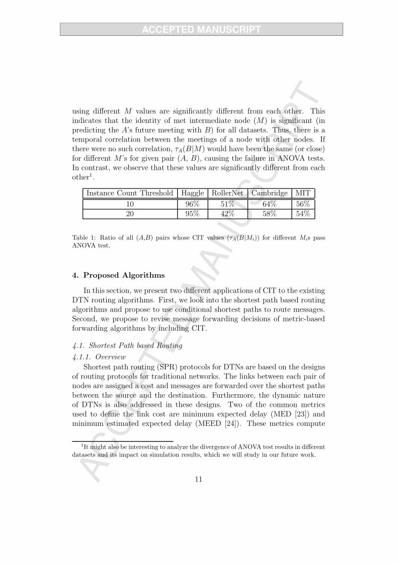
using different M values are significantly different from each other. Thisindicates that the identity of met intermediate node (M) is significant (inpredicting the A’s future meeting with B) for all datasets. Thus, there is atemporal correlation between the meetings of a node with other nodes. Ifthere were no such correlation, τA(B|M) would have been the same (or close)for different M ’s for given pair (A, B), causing the failure in ANOVA tests.In contrast, we observe that these values are significantly different from eachother1.

Instance Count Threshold Haggle RollerNet Cambridge MIT

10 96% 51% 64% 56%20 95% 42% 58% 54%

Table 1: Ratio of all (A,B) pairs whose CIT values (τA(B|Mi)) for different Mis passANOVA test.

4. Proposed Algorithms

In this section, we present two different applications of CIT to the existingDTN routing algorithms. First, we look into the shortest path based routingalgorithms and propose to use conditional shortest paths to route messages.Second, we propose to revise message forwarding decisions of metric-basedforwarding algorithms by including CIT.

4.1. Shortest Path based Routing

4.1.1. Overview

Shortest path routing (SPR) protocols for DTNs are based on the designsof routing protocols for traditional networks. The links between each pair ofnodes are assigned a cost and messages are forwarded over the shortest pathsbetween the source and the destination. Furthermore, the dynamic natureof DTNs is also addressed in these designs. Two of the common metricsused to define the link cost are minimum expected delay (MED [23]) andminimum estimated expected delay (MEED [24]). These metrics compute

1It might also be interesting to analyze the divergence of ANOVA test results in differentdatasets and its impact on simulation results, which we will study in our future work.

11

the expected waiting time plus the transmission delay between each pair ofnodes. However, while the former uses the future contact schedule, the latteruses only observed contact history.

In SPR, routing decision can be made: i) at source node, ii) at each hop,and iii) at each contact with other nodes. The utilization of recent contactinformation increases from the first to the last one improving the quality ofthe forwarding decisions; however, more processing resources are used as therouting decisions are made more frequently.

The suitability of SPR algorithms for DTNs and the scalability and com-plexity of their designs have been already discussed in [23, 24], hence, in thispaper, we focus on the enhancements of the performance of SPR algorithmsachieved by utilizing our metric (CIT), rather than using SIT. To this end, inthe rest of this section, we show the necessary changes to the current designsof SPR algorithms.

4.1.2. Network Model

We model a DTN as a graph G = (V ′, E ′) where the mobile nodes arerepresented by vertices (V ′) and the possible connections between these nodesare represented by the edges. Unlike previous DTN graph models, since CITconsiders node relations with respect to a third node, we define V ′ and E ′

sets in a different way. Given V is the set of all node names and N(i) denotesthe set of other nodes that meet with node i (i.e. neighbors of node i):

V ⊆ V × V and E ′ ⊆ V ′ × V ′ where,

V ′ = {(ij) | ∀j ∈ N(i)}E ′ = {(ij , kl) | i = l}

where, w′(ij , kl) =

{τi(k|j) if j 6= kτi(k) otherwise

4.1.3. Conditional Shortest Path Routing

Our algorithm basically finds conditional shortest paths (CSP) for eachsource-destination pair and routes the messages over these paths. We definethe CSP < n0, n1, . . . , nd−1, nd > as follows:

CSP (n0, nd) = min

{ℜn0(n1|t) +

d−1∑

i=1

τni(ni+1|ni−1)

}

Here, t represents the time that has passed since the last meeting of n0 withn1 and ℜn0(n1|t) is the expected residual time to the next meeting of n0

12

and n1 given that they have not met in the last t time units. ℜn0(n1|t)can be computed as in [14] with parameters of distribution representing theintermeeting time between n0 and n1. It can also be approximated iterativelyfrom the observed intermeeting times of n0 and n1. Assume that n0 observedk intermeeting times with n1 in the past. Let τ 1

n0(n1), τ 2

n0(n1),. . .τ

kn0

(n1)denote these values. Then, at time t, the iterative computation of ℜn0(n1|t)can be defined formally as follows:

ℜn0(n1|t) =

∑ks=1 f s

n0(n1)

|{τ sn0

(n1) ≥ t }| where,

f sn0

(n1) =

{τ sn0

(n1)− t if τ sn0

(n1) ≥ t0 otherwise

If none of the k observed intermeeting times is bigger than t (this case is lesslikely to occur as the contact history grows), ℜn0(n1|t) is set to 0, which is agood approximation.

Each node forms the DTN using the aforementioned network model andcollects SIT and CIT information of other nodes via epidemic link stateprotocol as it is described in the original study [24]. Note that, thanks tothe design of aforementioned network model which provides only valid CSPpaths between nodes, running Dijkstra’s or Bellman-Ford algorithm on thecurrent graph structure gives us the correct CSPs for each source destinationpair.

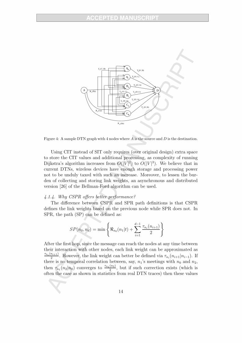
In Figure 4, we show a sample DTN graph where all mobile nodes A toD meet with each other and we set the source node to A and destinationnode to D (unused edges are not shown for brevity). Note that the graphincludes all possible paths from A to D and does not contain unlikely edgeslike (CD, DA). Hence, only the correct τ values will be added to the pathcalculation. To solve the CSP problem however, we add one vertex for sourceS and one vertex for destination node D. We also add outgoing edges from Sto each vertex (iS) ∈ V ′ with weight ℜS(i|t). Furthermore, for the destinationnode, D, we only add incoming edges from each vertex ij ∈ V ′ with weightτi(D|j) and from S with weight ℜS(D|t).

Running Dijkstra’s shortest path algorithm on G′ given the source nodeS and destination node D will give the shortest conditional path. In G,|V ′| = O(|V |2) and |E ′| = O(|V 3|), thus, Dijkstra’s algorithm will run inO(|V |3) (with Fibonacci heaps) while computing the original shortest paths(with SIT and simple DTN graphs) takes O(|V |2).

13

BA

BC

CA

CB

AB

AC

DA

A(D|t)

A(C|t)

A(B|t)

C

(C | B)

C(B | A)

(D | B)

A

B(A | C)

A(D | B)

A(D | C)

B(D | C)

C(D | A)

B(D | A)

T

T

T

T

T

T

T

T

T

R

R

R

Figure 4: A sample DTN graph with 4 nodes where A is the source and D is the destination.

Using CIT instead of SIT only requires (over original design) extra spaceto store the CIT values and additional processing, as complexity of runningDijkstra’s algorithm increases from O(|V |2) to O(|V |3). We believe that incurrent DTNs, wireless devices have enough storage and processing powernot to be unduly taxed with such an increase. Moreover, to lessen the bur-den of collecting and storing link weights, an asynchronous and distributedversion [26] of the Bellman-Ford algorithm can be used.

4.1.4. Why CSPR offers better performance?

The difference between CSPR and SPR path definitions is that CSPRdefines the link weights based on the previous node while SPR does not. InSPR, the path (SP) can be defined as:

SP (n0, nd) = min

{ℜn0(n1|t) +

d−1∑

i=1

τni(ni+1)

2

}

After the first hop, since the message can reach the nodes at any time betweentheir interaction with other nodes, each link weight can be approximated asτni

(ni+1)

2. However, the link weight can better be defined via τni

(ni+1|ni−1). Ifthere is no temporal correlation between, say, n1’s meetings with n0 and n2,

then τn1(n2|n0) converges toτn1 (n2)

2, but if such correction exists (which is

often the case as shown in statistics from real DTN traces) then these values

14

will be different and routing via CSPR will therefore be faster2.

4.2. Metric-based Forwarding Algorithms

4.2.1. Overview

A common method of routing in DTNs is to forward the message tothe encountered node that is more likely to meet with destination than thecurrent message carrier. However, making effective forwarding decisions insingle-copy based routing in DTNs is a challenging task. When two nodesmeet, one of them forwards a message to the other one if it decides that themessage will have a higher chance to be delivered to the destination at theother node.

In previous work, depending on the observed contact history betweennodes, several metrics have been used to define the delivery quality of nodes.Popular ones include encounter frequency [2], time elapsed since last en-counter [16]-[17], residual time [14] and social similarity [18] [19].

4.2.2. Proposed Modification

In most of the previous work, meetings of a node with other nodes areassumed independent from each other and the forwarding decision at theencounter of two nodes is made depending on their individual relations withthe destination node. In some algorithms such as [2] [17], with additionalprocessing (i.e. applying transitivity) on pairwise meetings, more accuratemetrics are used to reflect the effect of other nodes on the delivery qualityof a node. However, these improvements can also be applied to all othermetrics, including the one introduced in this paper. Our contribution is theintroduction of a new metric having this property by default in its basicdefinition.

To make forwarding decisions of these algorithms more effective, thus toimprove their performance, we propose to use CIT as an additional deliverymetric. That is, when two nodes meet, they will also compare their CITwith destination (depending on the condition that they met each other). If

2It is should be noted that the values of τ function are approximated iteratively. How-ever they are used to select the minimum delay paths, so the error of selection is boundedby the error of approximation. In other words, if iterative averages are close to each other,so are the real averages, thus wrong selection will have small impact on performance.Moreover, such an error of selection arises in all routing methods using the iterativelyapproximated averages. Thus, this error does not negate the improvements of CSPR.

15

the current carrier of the message learns that other node also has a shorterremaining time (according to CIT) to meet the destination than itself, themessage is forwarded. This additional condition eliminates forwardings thatbased on CIT became harmful and if executed would decrease the deliveryprobability. Simulation results confirm this conclusion, as the delivery ratesare preserved and simply unbeneficial forwardings are not performed. There-fore, more effective forwarding decisions are made so that the cost of messagedelivery declines while the delivery ratio and average delay are maintained(in some cases, even the delivery ratio increases and average delay decreases).

4.2.3. Why modification offers better performance?

With the addition of CIT as second forwarding condition, forwarding de-cisions are made depending on both the pairwise node relations between Aand B (due to the metric of original algorithm) and also possible temporalcorrelations between the meetings of A with nodes M and B. If there isno such correlation, CIT often supports the forwarding if the original metricalso supports the forwarding. However, when this correlation is strong, CIToffers more accurate prediction and it may indicate that at the time of themeeting the forwarding is no longer beneficial. Thus, the statistically harmfulforwarding decisions without considering possible correlations are prevented.Even though addition of CIT makes modified algorithms more selective, themessages are forwarded to or stay with the nodes which have higher deliv-ery probability at the time of the meeting with node M3. Thus, deliveryperformance stays similar or improves while the cost (i.e., the number offorwardings) decreases, yielding better routing efficiency.

5. Performance Evaluation

To evaluate the performance of proposed algorithms, we have built aJava based custom DTN simulator. It uses either the traces of real objectsfrom real DTN environments or the traces which are built synthetically. Thenetwork parameters (number of nodes etc.) are set according to the tracesused.

3Note that the path to delivery in modified algorithms can be totally different than thepath in original algorithms. In original algorithm A may forward the message to M1 butin modified version, A may skip M1 due to the unsatisfied CIT condition and later forwardthe message to M2 which satisfies both conditions. The remaining paths of the messagetowards the destination in both cases are likely to continue to be partially disjoint.

16

5.1. Algorithms in Comparison

We compared existing DTN algorithms with their CIT-using modifiedversions. First, we compared Shortest Path Routing (SPR) with Condi-tional Shortest Path Routing (CSPR) which is described in Section 4.1.3.Then, we compared the existing and revised versions of three metric-basedDTN routing algorithms: Prophet [2], Fresh [16] and SimBet [18]. In therevised versions of these algorithms (referred to as C-Prophet, C-Fresh andC-SimBet to underline that they use CIT), A forwards the message to B ifτA(D|B) > τB(D|A) is also satisfied (in addition to algorithm’s own forward-ing condition). In the graphs, we also give the results obtained by EpidemicRouting [6] since it achieves the optimum delivery ratio and delay (at highcost, however).

5.2. Data Sets

For the main simulations, we used three real and one synthetic DTNtraces. Real traces are from RollerNet [15], Cambridge [28] and Haggle [30]datasets where Bluetooth sightings between respectively 62, 36 and 41 usermobile devices are recorded. Further details of these traces can be foundin crawdad archive [29]. Synthetic traces are generated using a community-based mobility model which is similar to the models in [20, 21, 25]. In a 1000units by 1000 units square region, we generated Nc randomly located non-overlapping community regions (home, work, school etc.) of size 100 unitsby 100 units and distributed Np nodes (i.e. people) to these communityregions. For each node, we randomly assigned V communities to visit (i.e.commonly visited places for a person in a day). Each node first selects arandom point within the next community region in its list, assigns a randomspeed in range [Vmin, Vmax] and moves towards the target point with thatspeed. Once it reaches that point, it randomly assigns a visit duration inrange [Tmin, Tmax] and randomly walks within the community region for thatvisit duration. Once that duration expires, it moves to the next communityin its list in a similar way. Each node visits all the communities in its listas indicated, then once all of them are done (i.e. end of day), they againstart the same process and start visiting the communities in their list. Whilenodes are moving, we record the meetings between nodes assuming theyhave a transmission range of R. The default values for the parameters areNc=10, Np=50, V =5, Vmin=10 units, Vmax=50 units, Tmin=20 time units,Tmax=50 time units. However, we also looked at the effects of different values

17

0 10 20 30 40 500

0.2

0.4

0.6

0.8

1

Time (min)

Me

ssa

ge

de

live

ry r

atio

SPRCSPREpidemic

(a) RollerNet traces

0 1 2 3 4 5 60

0.2

0.4

0.6

0.8

1

Time (day)M

essa

ge

de

live

ry r

atio

SPRCSPREpidemic

(b) Cambridge traces

0 0.5 1 1.5 20

0.2

0.4

0.6

0.8

1

Time (day)

Me

ssa

ge

de

live

ry r

atio

SPRCSPREpidemic

(c) Haggle traces

0 100 200 300 400 5000

0.2

0.4

0.6

0.8

1

Time units

Me

ssa

ge

de

live

ry r

atio

SPRCSPREpidemic

(d) Synthetic traces

RollerNet Cambridge Haggle Synthetic0

0.2

0.4

0.6

0.8

1

1.2

1.4

1.6

1.8

2

Ave

rage

cos

t per

mes

sage

SPRCSPR

(e) Average Cost

RollerNet Cambridge Haggle Synthetic0

0.1

0.2

0.3

0.4

0.5

0.6

Rou

ting

Effi

cien

cy

SPRCSPR

(f) Routing Efficiency

Figure 5: Comparison of SPR and CSPR: Message delivery ratio (a-d), Cost (e) andRouting Efficiency (f).

of parameters in simulations. We also used large scale WiFi traces [34] toevaluate the performance of the proposed approach in large scale networks.

5.3. Simulation Results

To collect several routing statistics, we have generated traffic on the afore-mentioned traces. For each simulation run, after a warm up period4 (20%of the data), we generated 5000 messages from a random source node to arandom destination node at each t seconds. In RollerNet, since the durationof experiment is short, we set t = 1s, but for Cambridge and Haggle datasets, we set t = 1min and t = 30s, respectively. For synthetic trace, we sett = 10 time units. Besides this single difference, we compare all algorithmsin the same conditions.

4During warm up period, nodes build some encounter history to compute their initialCIT values. After the warm up period, as the messages are received and new meetingshappen, CIT values are updated in parallel and the forwarding decisions are performedusing the updated CIT values.

18

0 10 20 30 40 500

0.2

0.4

0.6

0.8

1

Time (min)

Me

ssa

ge

de

live

ry r

atio

ProphetC−ProphetFreshC−FreshSimBetC−SimBetEpidemic

(a) Delivery ratio

5 10 15 20 25 30 35 40 45 500

5

10

15

20

Time (min)A

ve

rag

e C

ost

ProphetC−ProphetFreshC−FreshSimBetC−SimBet

(b) Average cost

0 10 20 30 40 500

0.1

0.2

0.3

0.4

0.5

Time (min)

Ro

utin

g E

ffic

ien

cy

(c) Routing efficiency

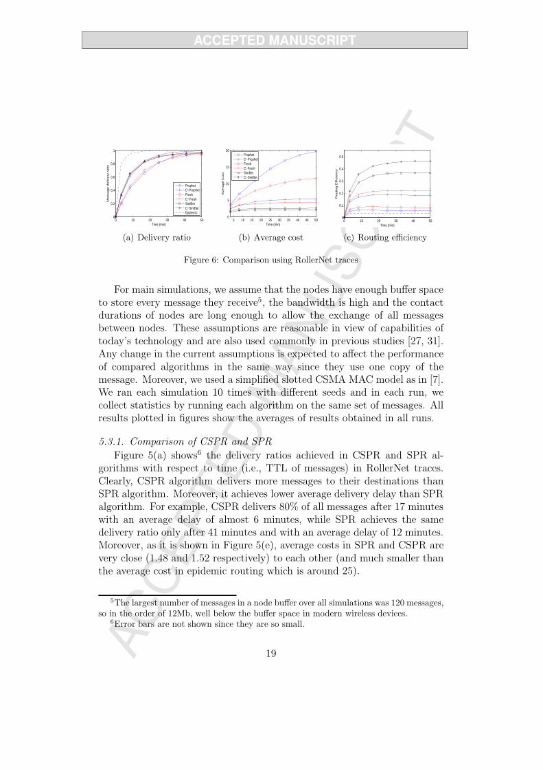
Figure 6: Comparison using RollerNet traces

For main simulations, we assume that the nodes have enough buffer spaceto store every message they receive5, the bandwidth is high and the contactdurations of nodes are long enough to allow the exchange of all messagesbetween nodes. These assumptions are reasonable in view of capabilities oftoday’s technology and are also used commonly in previous studies [27, 31].Any change in the current assumptions is expected to affect the performanceof compared algorithms in the same way since they use one copy of themessage. Moreover, we used a simplified slotted CSMA MAC model as in [7].We ran each simulation 10 times with different seeds and in each run, wecollect statistics by running each algorithm on the same set of messages. Allresults plotted in figures show the averages of results obtained in all runs.

5.3.1. Comparison of CSPR and SPR

Figure 5(a) shows6 the delivery ratios achieved in CSPR and SPR al-gorithms with respect to time (i.e., TTL of messages) in RollerNet traces.Clearly, CSPR algorithm delivers more messages to their destinations thanSPR algorithm. Moreover, it achieves lower average delivery delay than SPRalgorithm. For example, CSPR delivers 80% of all messages after 17 minuteswith an average delay of almost 6 minutes, while SPR achieves the samedelivery ratio only after 41 minutes and with an average delay of 12 minutes.Moreover, as it is shown in Figure 5(e), average costs in SPR and CSPR arevery close (1.48 and 1.52 respectively) to each other (and much smaller thanthe average cost in epidemic routing which is around 25).

5The largest number of messages in a node buffer over all simulations was 120 messages,so in the order of 12Mb, well below the buffer space in modern wireless devices.

6Error bars are not shown since they are so small.

19

0 1 2 3 40

0.2

0.4

0.6

0.8

1

Time (day)

Me

ssa

ge

de

live

ry r

atio

ProphetC−ProphetFreshC−FreshSimBetC−SimBetEpidemic

(a) Delivery ratio

0.5 1 1.5 2 2.5 3 3.5 4 4.50

1

2

3

4

5

6

7

8

Time (day)A

ve

rag

e C

ost

ProphetC−ProphetFreshC−FreshSimBetC−SimBet

(b) Average cost

0 1 2 3 40

0.1

0.2

0.3

0.4

0.5

Time (day)

Ro

utin

g E

ffic

ien

cy

(c) Routing efficiency

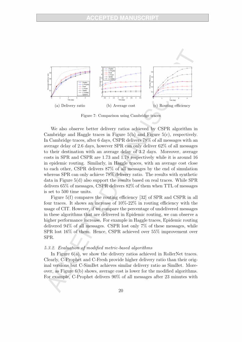
Figure 7: Comparison using Cambridge traces

We also observe better delivery ratios achieved by CSPR algorithm inCambridge and Haggle traces in Figure 5(b) and Figure 5(c), respectively.In Cambridge traces, after 6 days, CSPR delivers 78% of all messages with anaverage delay of 2.6 days, however SPR can only deliver 62% of all messagesto their destination with an average delay of 3.2 days. Moreover, averagecosts in SPR and CSPR are 1.73 and 1.78 respectively while it is around 16in epidemic routing. Similarly, in Haggle traces, with an average cost closeto each other, CSPR delivers 87% of all messages by the end of simulationwhereas SPR can only achieve 78% delivery ratio. The results with syntheticdata in Figure 5(d) also support the results based on real traces. While SPRdelivers 65% of messages, CSPR delivers 82% of them when TTL of messagesis set to 500 time units.

Figure 5(f) compares the routing efficiency [32] of SPR and CSPR in allfour traces. It shows an increase of 10%-22% in routing efficiency with theusage of CIT. However, if we compare the percentage of undelivered messagesin these algorithms that are delivered in Epidemic routing, we can observe ahigher performance increase. For example in Haggle traces, Epidemic routingdelivered 94% of all messages. CSPR lost only 7% of these messages, whileSPR lost 16% of them. Hence, CSPR achieved over 55% improvement overSPR.

5.3.2. Evaluation of modified metric-based algorithms

In Figure 6(a), we show the delivery ratios achieved in RollerNet traces.Clearly, C-Prophet and C-Fresh provide higher delivery ratio than their orig-inal versions but C-SimBet achieves similar delivery ratio as SimBet. More-over, as Figure 6(b) shows, average cost is lower for the modified algorithms.For example, C-Prophet delivers 90% of all messages after 23 minutes with

20

0 0.5 1 1.5 20

0.2

0.4

0.6

0.8

1

Time (day)

Me

ssa

ge

de

live

ry r

atio

ProphetC−ProphetFreshC−FreshSimBetC−SimBetEpidemic

(a) Delivery ratio

0.5 1 1.5 20

5

10

15

20

Time (day)A

ve

rag

e C

ost

ProphetC−ProphetFreshC−FreshSimBetC−SimBet

(b) Average cost

0 0.5 1 1.5 20

0.1

0.2

0.3

0.4

0.5

Time (day)

Ro

utin

g E

ffic

ien

cy

(c) Routing efficiency

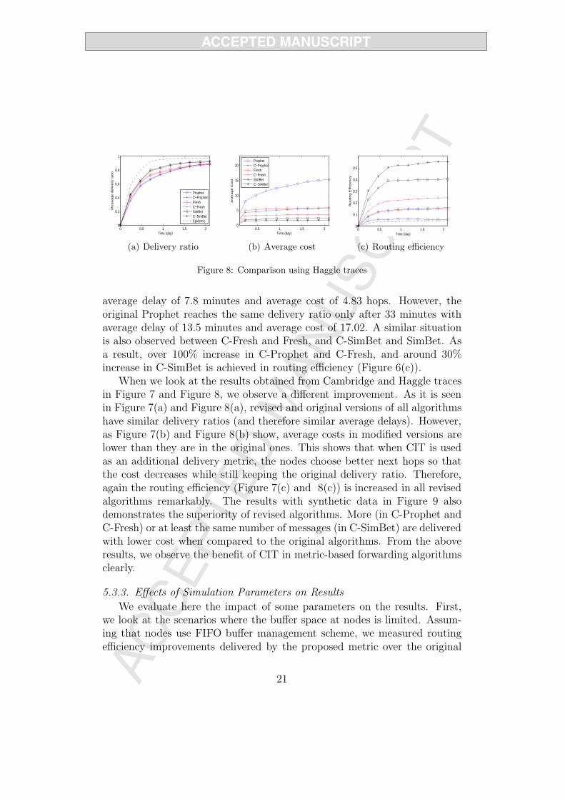
Figure 8: Comparison using Haggle traces

average delay of 7.8 minutes and average cost of 4.83 hops. However, theoriginal Prophet reaches the same delivery ratio only after 33 minutes withaverage delay of 13.5 minutes and average cost of 17.02. A similar situationis also observed between C-Fresh and Fresh, and C-SimBet and SimBet. Asa result, over 100% increase in C-Prophet and C-Fresh, and around 30%increase in C-SimBet is achieved in routing efficiency (Figure 6(c)).

When we look at the results obtained from Cambridge and Haggle tracesin Figure 7 and Figure 8, we observe a different improvement. As it is seenin Figure 7(a) and Figure 8(a), revised and original versions of all algorithmshave similar delivery ratios (and therefore similar average delays). However,as Figure 7(b) and Figure 8(b) show, average costs in modified versions arelower than they are in the original ones. This shows that when CIT is usedas an additional delivery metric, the nodes choose better next hops so thatthe cost decreases while still keeping the original delivery ratio. Therefore,again the routing efficiency (Figure 7(c) and 8(c)) is increased in all revisedalgorithms remarkably. The results with synthetic data in Figure 9 alsodemonstrates the superiority of revised algorithms. More (in C-Prophet andC-Fresh) or at least the same number of messages (in C-SimBet) are deliveredwith lower cost when compared to the original algorithms. From the aboveresults, we observe the benefit of CIT in metric-based forwarding algorithmsclearly.

5.3.3. Effects of Simulation Parameters on Results

We evaluate here the impact of some parameters on the results. First,we look at the scenarios where the buffer space at nodes is limited. Assum-ing that nodes use FIFO buffer management scheme, we measured routingefficiency improvements delivered by the proposed metric over the original

21

0 100 200 300 400 5000

0.2

0.4

0.6

0.8

1

Time units

Me

ssa

ge

de

live

ry r

atio

ProphetC−ProphetFreshC−FreshSimBetC−SimBetEpidemic

(a) Delivery ratio

0 100 200 300 400 5000

2

4

6

8

10

12

14

16

Time unitsA

ve

rag

e C

ost

ProphetC−ProphetFreshC−FreshSimBetC−SimBet

(b) Average cost

0 100 200 300 400 5000

0.1

0.2

0.3

0.4

0.5

Time units

Ro

utin

g E

ffic

ien

cy

(c) Routing efficiency

Figure 9: Comparison using Synthetic traces

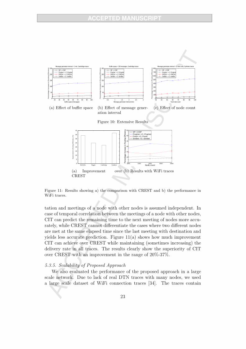
algorithms. Figure 10(a) shows the results for different buffer sizes in therange of [15-100] messages (in Cambridge traces). For these simulations wekept the message generation interval t=1 min and TTL=4 days. The resultsshow that in the modified versions of algorithms, the increase in the routingefficiency grows as the buffer space increases. Moreover, the increase con-verges to a constant value after sufficient buffer spaces is allocated. CSPR,C-SimBet, C-Fresh, and C-Prophet offer 22%, 26% 48% and 130% increasein the routing efficiency over their original algorithms, respectively.

In Figure 10(b), we observe similar results with different message gen-eration intervals. As the messages are generated more frequently, due tobuffer overflow, some messages are lost. However, the routing efficiency ofalgorithms is still remarkably increased with modified versions. Finally, wechanged the node count in the network (in synthetic traces) and looked at theeffect of node count on results. Figure 10(c) clearly shows that the increasein routing efficiency rises as the node count increases. This is because insynthetic data, temporal correlation between the meetings of nodes increasesdue to higher number of nodes in each community. Thus, CIT provides moreaccurate information about node relations.

5.3.4. Comparison with Closest Related Work

Even though several DTN routing algorithms have been proposed in lit-erature, they usually assume that the meetings of a node with other nodesare independent and identically distributed. The closest study to our workis in [14], where a new metric, conditional residual time (CREST), whichcomputes the remaining time for the meetings of two nodes based on thecondition that t time units has passed since their last encounter, is proposed.However, the relations with other nodes is still not considered in this compu-

22

20 30 40 50 60 70 80 90 1000

50

100

150

200

250

Buffer space (messages)

Pe

rce

nta

ge

In

cre

ase

in

Ro

utin

g E

ffic

ien

cy

Message generation interval = 1 min, Cambridge traces

SP −> CSPProphet −> C−ProphetFRESH −> C−FRESHSimBet −> C−SimBet

(a) Effect of buffer space

0.5 1 1.5 2 2.5 30

50

100

150

200

250

Message generation interval (min)P

erc

en

tag

e I

ncre

ase

in

Ro

utin

g E

ffic

ien

cy

Buffer space = 100 messages, Cambridge traces

SP −> CSPProphet −> C−ProphetFRESH −> C−FRESHSimBet −> C−SimBet

(b) Effect of message gener-ation interval

30 40 50 60 70 80 90 1000

100

200

300

400

500

600

700

800

Total node count

Pe

rce

nta

ge

In

cre

ase

in

Ro

utin

g E

ffic

ien

cy

Message generation interval = 10 time units, Synthetic traces

SP −> CSPProphet −> C−ProphetFRESH −> C−FRESHSimBet −> C−SimBet

(c) Effect of node count

Figure 10: Extensive Results

0

5

10

15

20

25

30

35

40

RollerNet Haggle Cambridge Synthetic

Impr

ovem

ent

in R

outi

ng E

ffic

ienc

y (%

)

(a) Improvement overCREST

1000 1500 2000 2500 30000

10

20

30

40

50

60

Node count

Per

cent

age

Incr

ease

in R

outin

g E

ffici

ency

SP−>CSPProphet−>C−ProphetFresh−>C−FreshSimbet−>C−Simbet

(b) Results with WiFi traces

Figure 11: Results showing a) the comparison with CREST and b) the performance inWiFi traces.

tation and meetings of a node with other nodes is assumed independent. Incase of temporal correlation between the meetings of a node with other nodes,CIT can predict the remaining time to the next meeting of nodes more accu-rately, while CREST cannot differentiate the cases where two different nodesare met at the same elapsed time since the last meeting with destination andyields less accurate prediction. Figure 11(a) shows how much improvementCIT can achieve over CREST while maintaining (sometimes increasing) thedelivery rate in all traces. The results clearly show the superiority of CITover CREST with an improvement in the range of 20%-37%.

5.3.5. Scalability of Proposed Approach

We also evaluated the performance of the proposed approach in a largescale network. Due to lack of real DTN traces with many nodes, we useda large scale dataset of WiFi connection traces [34]. The traces contain

23

587782 user sessions for 69689 (distinct) users, which were collected from206 hotspots for three years. We assumed that the users that are connectedto the same hotspot can communicate with each other to obtain the meetings(i.e. communication opportunity) of nodes similar to the DTN environment.There are many users which appear a few times in the dataset thus theirmeeting counts with other nodes is very small. Therefore, we first identifiedthe top 1000, 2000 and 3000 nodes having the most meetings and utilizedthe meeting history that occur among these nodes for the evaluation of theproposed approach. As the Figure 11(b) shows, the modified versions of al-gorithms has much better routing efficiency (with similar or higher deliveryrate) compared to the original algorithms. The increase achieved via modi-fied algorithms is smaller than the increase in routing efficiency shown in theresults with other datasets. This can be due to the difference of WiFi tracesthan DTN traces, however, the results show that proposed approach can pro-vide enough improvement even in large scale networks. CSPR, C-SimBet,C-Fresh, and C-Prophet algorithms offer 8%, 10% 17% and 30% increase onthe average in the routing efficiency over their original algorithms, respec-tively.

6. Conclusion and Future Work

In this paper, we focused on the routing problem in delay tolerant net-works (DTN). First, we introduced a new metric called conditional inter-meeting time (CIT) which is the average time that passes from the time anode meets with a neighbor until the time it meets another one. Next, wepresented an analysis of this metric showing why it can improve represen-tation accuracy of node relations. Then, we looked at the effects of thismetric on existing DTN routing algorithms. To this end, we modified theircurrent designs to enable them to use CIT. Finally, through extensive simu-lations based on both the real DTN traces and synthetic mobility traces, weevaluated the modified algorithms and demonstrated their superiority overoriginal ones.

In our future work, we plan to extend the definition of CIT to includemore than one meeting in the contact history. To achieve this, we plan to useprobabilistic context free grammars (PCFG) and the construction algorithmpresented in [35].

[1] T. Spyropoulos, K. Psounis, and C. S. Raghavendra, Efficient rout-

24

ing in intermittently connected mobile networks: The single-copy case,IEEE/ACM Transactions on Networking, vol. 16(1), Feb. 2008.

[2] A. Lindgren, A. Doria, and O. Schelen, Probabilistic routing in intermit-tently connected networks, SIGMOBILE Mobile Computing and Com-munication Review, vol. 7(3), 2003.

[3] J. Burgess, B. Gallagher, D. Jensen, and B. N. Levine, MaxProp: Rout-ing for Vehicle-Based Disruption- Tolerant Networks, In Proc. IEEEInfocom, April 2006.

[4] C. Mascolo, and M. Musolesi, CAR: Context-aware Adaptive Routingfor Delay Tolerant Mobile Networks, in IEEE Transactions on MobileComputing. Vol. 8(2), pp. 246-260. February 2009.

[5] E. Bulut, and B. K. Szymanski, Exploiting Friendship Relations for Effi-cient Routing in Mobile Social Networks, IEEE Transactions on Paralleland Distributed Systems, 23(12) 2012, pp. 2254-2265.

[6] A. Vahdat and D. Becker, Epidemic routing for partially connected adhoc networks, Duke University, Tech. Rep. CS-200006, 2000.

[7] T. Spyropoulos, K. Psounis,C. S. Raghavendra, Efficient routingin intermittently connected mobile networks: The multi-copy case,IEEE/ACM Transactions on Networking, 2008.

[8] A. Balasubramanian, B. N. Levine, A. Venkataramani, Replication Rout-ing in DTNs: A Resource Allocation Approach, IEEE Transactions onNetworking, Vol. 18(2), April 2010.

[9] Y. Wang, S. Jain, M. Martonosi, and K. Fall, Erasure coding based rout-ing for opportunistic networks, in Proc. of ACM SIGCOMM workshopon Delay Tolerant Networking (WDTN), 2005.

[10] E. Bulut, Z. Wang and B. K. Szymanski, Cost Efficient Erasure Cod-ing based Routing in Delay Tolerant Networks, in Proc. of the ICC,Capetown, South Africa, May 2010.

[11] I. Psaras, L. Wood and R. Tafazolli, Delay-/Disruption-Tolerant Net-working: State of the Art and Future Challenges, Technical Report,University of Surrey, UK, 2009.

25

[12] A. Chaintreau, P. Hui, J. Crowcroft, C. Diot, R. Gass, and J. Scott,Impact of Human Mobility on the Design of Opportunistic ForwardingAlgorithms, in Proc. of INFOCOM, 2006.

[13] X. Zhang, J. F. Kurose, B. Levine, D. Towsley, and H. Zhang, Study of aBus-Based Disruption Tolerant Network: Mobility Modeling and Impacton Routing, In Proc. of ACM MobiCom, 2007.

[14] S. Srinivasa and S. Krishnamurthy, CREST: An Opportunistic Forward-ing Protocol Based on Conditional Residual Time, in Proc. of SECON,2009.

[15] P. U. Tournoux, J. Leguay, F. Benbadis, V. Conan, M. Amorim, J. Whit-beck, The Accordion Phenomenon: Analysis, Characterization, and Im-pact on DTN Routing, in Proc. of Infocom, 2009.

[16] H. Dubois-Ferriere, M. Grossglauser, and M. Vetterli, Age Matters: Ef-ficient Route Discovery in Mobile Ad Hoc Networks Using EncounterAges, In Proc. of ACM MobiHoc, 2003.

[17] T. Spyropoulos, K. Psounis, and C. Raghavendra, Spray and Focus: Ef-ficient Mobility-Assisted Routing for Heterogeneous and Correlated Mo-bility, In Proc. of IEEE PerCom, 2007.

[18] E. Daly and M. Haahr, Social Network Analysis for Information Flow inDisconnected Delay-Tolerant MANETs, in IEEE Transactions on MobileComputing, vol. 8(5), May, 2009.

[19] P. Hui, J. Crowcroft, and E. Yoneki, BUBBLE Rap: Social Based For-warding in Delay Tolerant Networks, In Proc. of ACM MobiHoc, 2008.

[20] F. Li, J. Wu, LocalCom: A Community-Based Epidemic ForwardingScheme in Disruption-tolerant Networks, in Proc. of IEEE Secon 2009.

[21] W. Hsu, T. Spyropoulos, K. Psounis, and A. Helmy, Modeling timevariant user mobility in wireless mobile networks, in IEEE INFOCOM,2007.

[22] C. Liu and J. Wu, Practical Routing in a Cyclic MobiSpace, InIEEE/ACM Transactions on Networking, vol.19(2), April, 2011.

26

[23] S. Jain, K. Fall, and R. Patra, Routing in a delay tolerant network, inProc.of ACM SIGCOMM, Aug. 2004.

[24] E. P. C. Jones, L. Li, and P. A. S. Ward, Practical routing in delay toler-ant networks, in Proc. of ACM SIGCOMM workshop on Delay TolerantNetworking (WDTN), 2005.

[25] T. Spyropoulos, K. Psounis,C. S. Raghavendra, Performance Analysisof Mobility-assisted Routing, In Proc. of MobiHoc, 2006.

[26] D. Bertsekas, and R. Gallager, Data networks (2nd ed.), 1992.

[27] C. Liu and J. Wu, On Multicopy Opportunistic Forwarding Protocolsin Nondeterministic Delay Tolerant Networks, in IEEE Transactions onParallel Dist. Syst., 23(6): 1121-1128, 2012.

[28] J. Leguay, A. Lindgren, J. Scott, T. Friedman, J. Crowcroft and P. Hui,CRAWDAD data set upmc/content (v. 2006-11-17), downloaded fromhttp://crawdad.cs.dartmouth.edu, 2006.

[29] CRAWDAD data set, http://crawdad.cs.dartmouth.edu..

[30] A European Union funded project in Situated and Autonomic Commu-nications, www.haggleproject.org.

[31] E. Bulut, Z. Wang, and B. Szymanski, Cost-Effective Multi-PeriodSpraying for Routing in Delay Tolerant Networks, in IEEE/ACM Trans-actions on Networking, Vol. 18(5), Oct. 2010.

[32] J. M. Pujol, A. L. Toledo, and P. Rodriguez, Fair routing in delay tol-erant networks, in Proc. of Infocom, 2009.

[33] S. Jain, M. Demmer, R. Patra, K. Fall, Using redundancy to cope withfailures in a delay tolerant network, in Proc. of ACM Sigcomm 2005.

[34] M. Lenczner, B. Grgoire and F. Proulx, CRAWDAD traceset ilesansfil/wifidog/session (v. 2007-08-27), downloaded fromhttp://crawdad.cs.dartmouth.edu/ilesansfil/wifidog/session, July, 2013.

[35] S. Geyik, E. Bulut and B. Szymanski, Grammatical Inference for Mod-eling Mobility Patterns in Networks, accepted to appear in IEEE Trans-actions on Mobile Computing (TMC), 2012.

27

[36] N. Eagle, A. Pentland, and D. Lazer, Inferring Social Network Structureusing Mobile Phone Data, in Proc. of National Academy of Sciences,106(36), pp. 15274-15278, 2009.

[37] E. Bulut, S. Geyik and B. Szymanski, Efficient Routing in Delay Tol-erant Networks with Correlated Node Mobility, in Proc. of MASS, Nov,2010.

[38] EasyFit: Distribution Fitting Software, http://www.mathwave.com/,last accessed in August, 2013.

28