Embed Size (px)
Citation preview

Utilization of Genetic Algorithms and Constrained Multivariable
Function Minimization to Estimate Load Model Parameters
from Disturbance Data
Christopher G. Mertz
Thesis submitted to the faculty of the Virginia Polytechnic Institute and State University in
partial fulfillment of the requirements for the degree of
Master of Science
In
Electrical Engineering
Jaime De La Ree Lopez, Chair
Arun G. Phadke
Virgilio A. Centeno
June 6th
, 2013
Blacksburg, VA
Keywords: Genetic Algorithms, Induction Motors,
Load Modeling, Power System Dynamics

Utilization of Genetic Algorithms and Constrained Multivariable
Function Minimization to Estimate Load Model Parameters
from Disturbance Data
Christopher G. Mertz
Abstract
As the requirements to operate the electric power system become more stringent
and operating costs must be kept to a minimum, operators and planners must ensure that power
system models are accurate and capable of replicating system disturbances. Traditionally, load
models were represented as static ZIP models; however, NERC has recently required that
planners model the transient dynamics of motor loads to study their effect on the post-
disturbance behavior of the power system. Primarily, these studies are to analyze the effects of
fault-induced, delayed voltage recovery, which could lead to cascading voltage stability issues.
Genetic algorithms and constrained multivariable function minimization are global and
local optimization tools used to extract static and dynamic load model parameters from post-
disturbance data. The genetic algorithm’s fitness function minimizes the difference between
measured and calculated real and reactive power by varying the model parameters. The fitness
function of the genetic algorithm, a function of voltage and frequency, evaluates an individual’s
difference between measured and simulated real and reactive power.
While real measured data was unavailable, simulations in PSS/E were used to create data,
and then compared against estimated data to examine the algorithms’ ability to estimate
parameters.

iii
To my parents, Dan and Sherry Mertz, and my brother, Alex Mertz, for helping shape me into
the person I am today.

iv
Acknowledgements
I would like to thank Dr. Jaime De La Ree for his support during my research. During my
six-year duration at Virginia Tech, his door was always open and he was always welcoming to
any questions I had, including my countless questions about machines. I would also like to
thank Dr. Virgilio Centeno and Dr. Arun Phadke for their willingness to sit on my committee and
be accommodating as I finished my research here at Virginia Tech.
I would like to thank Dominion Virginia Power for making my Graduate School
experience possible by providing my funding, especially Dr. Matthew Gardner and Kyle Thomas
for questions I had pertaining to the Fellowship and by offering guidance and wisdom.
I would like to thank my peers in the Power Lab at Virginia Tech for support when I had
technical questions and the friendship that you have provided. I certainly can’t thank you all
enough. Without you all, I certainly wouldn’t be where I am today.

v
Table of Contents
Abstract ............................................................................................................................. iii
Acknowledgements .......................................................................................................... iv
Table of Contents .............................................................................................................. v
List of Figures .................................................................................................................. vii
Chapter 1: Introduction .................................................................................................. 1
1.1 Basics of Load Modeling ...........................................................................................9
1.2 Types of Loads ...........................................................................................................9
1.2.1 Static Load Models ............................................................................................10
1.2.2 Dynamic Load Models ......................................................................................12
1.3 Component versus Measurement-Based Approach .................................................13
Chapter 2: Induction Motor Modeling ........................................................................ 16
2.1 Basic Single Phase Induction Machine Model ........................................................20
2.2 Three Phase Induction Motor with Flux Linkages ..................................................24
2.2.1 Voltage Equations in Machine Variables ..........................................................25
2.2.2 Machine Equations in the Arbitrary Reference Frame ......................................28
2.3 Induction Machine Modeling for Stability Analysis ...............................................34
Chapter 3: Optimization Algorithms ........................................................................... 37
3.1 The Genetic Algorithm ............................................................................................39
3.2 Constrained Multivariable Function Minimization .................................................42
Chapter 4: Load Modeling ............................................................................................ 44
4.1 Load Modeling in Software .....................................................................................45
4.1.1 Models in PSS/E ................................................................................................45
4.2 Sample Simulation Difference between PSS/E and DSA Tools .............................50

vi
Chapter 5: Implementation of Optimization Algorithms for Load Parameter Estimation
........................................................................................................................................... 54
5.1 Results ......................................................................................................................57
5.1.1 Static Load .........................................................................................................59
5.1.2 Small Motor Parameters at 100% Load.............................................................62
5.1.3 Large Motor Parameters at 100% Load.............................................................66
5.1.4 Small Motor Parameters at 50% Load...............................................................70
5.1.5 Custom Motor Parameters at 100% Load .........................................................74
5.1.6 Custom Motor Parameters 30%.........................................................................76
5.2 Discussion of Results ...............................................................................................78
5.3 Equal Area Criterion – Swinging of Synchronous Machines ..................................79
Chapter 6: Future Work ............................................................................................... 86
6.1 Voltage Stability ......................................................................................................87
6.2 Fault Induced Delayed Voltage Recovery (FIDVR) ...............................................89
References ........................................................................................................................ 91
Appendix A – MATLAB Code: ..................................................................................... 95

vii
List of Figures
Figure 1.1: Chart of Dynamic Stability Classifications within Power Systems [3]....................... 2
Figure 1.2: Incidents with Voltage Collapse around the World [5]. .............................................. 3
Figure 1.3: Map of Regions (Colored Areas) and Balancing Authorities (Circles) in the United
States [18]. ...................................................................................................................................... 5
Figure 1.4: The Measurement-Based Approach uses Measured Voltage, ..................................... 6
Frequency, and Real and Reactive Power to Formulate an Load Model [22]. ............................... 6
Figure 1.5: A Weighted Multilayer Perceptron Neural Network [28]. .......................................... 7
Figure 1.2.1: Behavior of ZIP Components with Varying Voltage. ............................................ 11
Figure 1.3.1: Component-Based Approach Uses Data for Individual Components to ................ 13
Form an Aggregate Load at the Bus. ............................................................................................ 13
Figure 1.3.2: Component-Based Approach Data for Various Load Components [3]. ................ 14
Figure 1.3.3: Aggregate Composition for Load Classes in the Component-Based Approach [3].
....................................................................................................................................................... 14
Figure 2.1: Example of a Stator and Rotor from an Induction Machine [36]. ............................. 16
Figure 2.2: An Example of a Three-Phase, Six-Pole Machine [36]. ........................................... 17
Figure 2.3: Typical Induction Motor Parameters in Per-Unit [31] [37]. ..................................... 18
Figure 2.4: Typical Induction Machine Parameters for Motor Analysis [38]. ............................ 19
Figure 2.1.1: Circuit for Induction machine Analysis with Losses Labeled. .............................. 21
Figure 2.1.2: 1) Take the Thévenin Equivalent Voltage Applied to the Rotor [35]. ................... 21
Figure 2.1.3: 2) Take the Thévenin Impedance of the Stator [35]. .............................................. 22
Figure 2.1.4: The Simplified Circuit of an Induction Machine [35]. ........................................... 22
Figure 2.1.5: Real Power Plot of a First-Order Induction Machine Simulation including .......... 23
Starting and a .05 Second (3 Cycle) Disturbance at 5 Seconds. ................................................... 23
Figure 2.1.6: Reactive Power Plot of a First-Order Induction Machine Simulation ................... 24
including Starting and a .05 Second (3 Cycle) Disturbance at 5 Seconds. ................................... 24
Figure 2.2.2.1: Real Power Plot of a Fifth-Order Induction Machine Simulation including
Starting and a .05 Second (3 Cycle) Disturbance at 5 Seconds. ................................................... 33

viii
Figure 2.2.2.2: Reactive Power Plot of a Fifth-Order Induction Machine Simulation including
Starting and a .05 Second (3 Cycle) Disturbance at 5 Seconds. ................................................... 33
Figure 2.3.1: Real Power Plot of a Fifth-Order Induction Machine Simulation including Starting
and a .05 Second (3 Cycle) Disturbance at 5 Seconds. ................................................................. 35
Figure 2.3.2: Reactive Power Plot of a Fifth-Order Induction Machine Simulation including
Starting and a .05 Second (3 Cycle) Disturbance at 5 Seconds. ................................................... 36
Figure 3.1: Classification of Global Optimization Techniques [39]............................................ 37
Figure 3.2: Evaluation of Local and Global Optimization Techniques [39]. .............................. 38
Figure 3.1.1: Populations are Made Up Chromosomes, the Possible Solutions for the Problem
[41]. ............................................................................................................................................... 39
Figure 3.1.2: Structure of the Genetic Algorithm Implementation [42]. ...................................... 40
Figure 3.1.3: Examples of Single-Point, Two-Point, or Multi-Point Crossover [41]. ................. 41
Figure 3.1.4: Examples of Single-Point, Group, or Multi-Point Mutation [41]. ......................... 41
Figure 4.1: Power System Components that Affect Voltage Stability [5]. .................................. 44
Figure 4.1.1.1: Type 1 and Type 2 Used in CIMWBL, CIM5BL, and CIM6BL models in PSS/E
[45]. ............................................................................................................................................... 46
Figure 4.1.1.2: Model Equations for Induction Motor Types 1 and 2 in PSS/E [46]. ................. 47
Figure 4.1.1.3: CLODBL is a Composite Load Model from PSS/E............................................ 50
Figure 4.1.1.4: CLODBL Motor Data for a Large Induction Motor. .......................................... 50
Figure 4.1.1.5: CLODBL Motor Data for a Small Induction Motor. .......................................... 50
Figure 4.2.1: Transient Voltage Comparison between PSS/E and DSA Tools. .......................... 51
Figure 4.2.2: Transient Frequency Comparison between PSS/E and DSA Tools. ...................... 52
Figure 4.2.3: Transient Real Power Comparison between PSS/E and DSA Tools. .................... 52
Figure 4.2.4: Transient Reactive Power Comparison between PSS/E and DSA Tools. .............. 53
Figure 4.2.5: CIM5BL Induction Motor Data Used in Simulations for PSS/E and DSA Tools. 53
Figure 5.1: Load Model Setup for Evaluation and Analysis within the Optimization Algorithms.
....................................................................................................................................................... 54
Figure 5.2: Single-Cage Induction Motor Model used in Simulation. ........................................ 55
Figure 5.1.1.1: Genetic Algorithm Best Individual and Fitness Value for Each Generation of the
Static Load. ................................................................................................................................... 59

ix
Figure 5.1.1.2: Reactive Power Plot of Optimization Output and PSS/E Output for the Static
Load Simulation. ........................................................................................................................... 60
Figure 5.1.1.3: Real Power Plot of Optimization Output and PSS/E Output for the Static Load
Simulation. .................................................................................................................................... 60
Figure 5.1.2.1: Genetic Algorithm Best Individual and Fitness Value for Each Generation of the
100% Small Motor Load Simulation. ........................................................................................... 62
Figure 5.1.2.2: Reactive Power Plot of Optimization Output and PSS/E Output for 100% Small
Motor Load Simulation. ................................................................................................................ 62
Figure 5.1.2.3: Real Power Plot of Optimization Output and PSS/E Output for 100% Small
Motor Load Simulation. ................................................................................................................ 63
Figure 5.1.2.4: Genetic Algorithm Best Individual and Fitness Value for Each Generation of the
100% Small Motor Load Simulation. ........................................................................................... 64
Figure 5.1.2.5: Reactive Power Plot of Optimization Output and PSS/E Output for 100% Small
Motor Load Simulation. ................................................................................................................ 64
Figure 5.1.2.6: Real Power Plot of Optimization Output and PSS/E Output for 100% Small
Motor Load Simulation. ................................................................................................................ 65
Figure 5.1.3.1: Genetic Algorithm Best Individual and Fitness Value for Each Generation of the
100% Large Motor Load Simulation. ........................................................................................... 66
Figure 5.1.3.2: Reactive Power Plot of Optimization Output and PSS/E Output for 100% Large
Motor Load Simulation. ................................................................................................................ 66
Figure 5.1.3.3: Real Power Plot of Optimization Output and PSS/E Output for 100% Large
Motor Load Simulation. ................................................................................................................ 67
Figure 5.1.3.4: Genetic Algorithm Best Individual and Fitness Value for Each Generation of the
100% Large Motor Load Simulation. ........................................................................................... 68
Figure 5.1.3.5: Reactive Power Plot of Optimization Output and PSS/E Output for 100% Large
Motor Load Simulation. ................................................................................................................ 68
Figure 5.1.3.6: Real Power Plot of Optimization Output and PSS/E Output for 100% Large
Motor Load Simulation. ................................................................................................................ 69
Figure 5.1.4.1: Genetic Algorithm Best Individual and Fitness Value for Each Generation of the
50% Small Motor Load Simulation. ............................................................................................. 70
Figure 5.1.4.2: Reactive Power Plot of Optimization Output and PSS/E Output for 50% Small
Motor Load Simulation. ................................................................................................................ 70
Figure 5.1.4.3: Real Power Plot of Optimization Output and PSS/E Output for 50% Small Motor
Load Simulation. ........................................................................................................................... 71

x
Figure 5.1.4.4: Genetic Algorithm Best Individual and Fitness Value for Each Generation of the
50% Small Motor Load Simulation. ............................................................................................. 72
Figure 5.1.4.5: Reactive Power Plot of Optimization Output and PSS/E Output for 50% Small
Motor Load Simulation. ................................................................................................................ 72
Figure 5.1.4.6: Real Power Plot of Optimization Output and PSS/E Output for 50% Small Motor
Load Simulation. ........................................................................................................................... 73
Figure 5.1.5.1: Genetic Algorithm Best Individual and Fitness Value for Each Generation of the
100% Custom Motor Load Simulation. ........................................................................................ 74
Figure 5.1.5.2: Reactive Power Plot of Optimization Output and PSS/E Output for 100%
Custom Motor Load Simulation. .................................................................................................. 74
Figure 5.1.5.3: Real Power Plot of Optimization Output and PSS/E Output for 100% Custom
Motor Load Simulation. ................................................................................................................ 75
Figure 5.1.6.1: Genetic Algorithm Best Individual and Fitness Value for Each Generation of the
30% Custom Motor Load Simulation. .......................................................................................... 76
Figure 5.1.6.2: Reactive Power Plot of Optimization Output and PSS/E Output for 30% Custom
Motor Load Simulation. ................................................................................................................ 76
Figure 5.1.6.3: Real Power Plot of Optimization Output and PSS/E Output for 30% Custom
Motor Load Simulation. ................................................................................................................ 77
Figure 5.3.1: Rotating Machine Connected to an Infinite Bus [48]. ............................................ 80
Figure 5.3.2: A Fixed-Point Pendulum and a Pendulum on a Rotating Mass. ............................ 81
Figure 5.3.3: Changing Conditions in a Motor Swinging with Respect to an Infinite Bus for a
Disturbance [48]............................................................................................................................ 82
Figure 5.3.4: Equal Area Criterion Applied to Fault Clearing when Parallel .............................. 82
Paths Provide for Power Transmission. ........................................................................................ 82
Figure 5.3.5: Voltage Angle Deviation during a Fault as Related to the Equal Area Criterion. . 84
Figure 5.3.6: Voltage Angle Difference Shows Stabilization between Load and Generator. ..... 84
Figure 6.1.1: Increase in Cost of Consumer Goods from 1985-2005 (Nominal Dollars) [49]. ... 87
Figure 6.1.2: Circuit Used For Maximum Power Transfer. ......................................................... 88

1
Chapter 1: Introduction
Today’s electric power grid has evolved into a highly complex network of generation
sources, transmission lines, and power system loads. Operators and users utilize conventional
generation methods, such as coal and natural gas, as well as contemporary generation methods of
solar and wind to supply power to a variety of loads. A mesh of AC and DC transmission lines
connect generation stations to loads which encompass everything from a simple light bulb in a
residential home, to complex electrical motors in an urban factory. Power utilities strive to
maintain highly reliable service to each customer while minimizing operating costs.
To keep service reliable, power system planners must model components within the
generation, transmission, and distribution (load) categories to perform studies on how the power
system will behave under various conditions. After modeling the components, the planners can
then use the modeled power system to run static or dynamic simulations to assess the stability of
the power system. Power system stability refers to the ability of synchronous machines
(generators) to move from one steady-state operating point to another steady-state operating
point, without losing synchronism [1].
Static simulations show steady-state operating conditions for the power system during a
snapshot in time. These simulations are good for hypothetical scenarios that change the
architecture of the power system either permanently or for a long period of time. For example, a
planner can see how adding or removing a transmission line between two nodes, called buses, in
the power system affect the loading on surrounding lines. Static simulations are used to ensure
that bus voltages are close to nominal values, phase angles of adjacent buses are similar, and
line-loading limits are not violated [2]. Three major line-loading limits are: (1) steady-state
stability limit, (2) thermal limit, and (3) voltage-drop limit. Dynamic simulations are used to
analyze how the system behaves over a period of time following a disturbance, such as a fault,
line-switching operation, or sudden loss of a generation or load. During a perturbation of the
power system, a mismatch in real and reactive power cause all rotating machinery to deviate
from their respective synchronous velocity due to voltage and frequency change. Dynamic
stability studies are performed to ensure that post-disturbance, machines will return to their

2
synchronous velocities with new steady-state power angles, and that voltage will recover in a
timely fashion.
Figure 1.1: Chart of Dynamic Stability Classifications within Power Systems [3]
Although power system operators strive for the utmost reliable service, perturbation
within the electric grid can require system operators to take drastic action to mitigate a severe
outage. In one particular incident in Western Tennessee, a persistent fault caused motor loads to

stall and draw a significant increase in react
power caused voltage to sag for 10 to 15 seconds before reverse zone 3 relays tripped
exacerbating the situation.
Figure 1.2: Incidents with Voltage Collapse
The remote zone 3 relays tripping
source lines in the area as well as transformer banks at three other substations due to low and
unbalanced voltages. Bullock, the author of the report, later said that several attempts were made
at replicating the voltage collapse event through simulation but none were successful
conventional ZIP load models. At the time
and more work needed to be done to analyze
Prior to the voltage collapse in Western Tennessee, in 1973 the Computer Analysis of
Power Systems Working Group of the Computer and Analytical
published a study citing that time constants of the loads were small enough to be negligible
3
stall and draw a significant increase in reactive power [4]. The excessive need for reactive
power caused voltage to sag for 10 to 15 seconds before reverse zone 3 relays tripped
Incidents with Voltage Collapse around the World [5].
The remote zone 3 relays tripping additional lines caused a cascading effect that tripped all
source lines in the area as well as transformer banks at three other substations due to low and
Bullock, the author of the report, later said that several attempts were made
at replicating the voltage collapse event through simulation but none were successful
. At the time, no guidelines had been set for dynamic load models
done to analyze the response to disturbances within the system.
Prior to the voltage collapse in Western Tennessee, in 1973 the Computer Analysis of
Power Systems Working Group of the Computer and Analytical Methods Subcommittee
published a study citing that time constants of the loads were small enough to be negligible
. The excessive need for reactive
power caused voltage to sag for 10 to 15 seconds before reverse zone 3 relays tripped,
caused a cascading effect that tripped all
source lines in the area as well as transformer banks at three other substations due to low and
Bullock, the author of the report, later said that several attempts were made
at replicating the voltage collapse event through simulation but none were successful using
dynamic load models
the response to disturbances within the system.
Prior to the voltage collapse in Western Tennessee, in 1973 the Computer Analysis of
Methods Subcommittee
published a study citing that time constants of the loads were small enough to be negligible [6].
4
The study also cited that resistive loads such as water heaters and electric ranges “swamp” small
motor load. Typical motor loads of the time consumed a max of 2,100 kWhr per year, while
resistive load was around 7,200 kWhr per year; thus using a static polynomial load model of the
form:
� = � + ���� +����
was satisfactory at the time. The polynomial static load model was generally considered
adequate for stability studies since most of the focus on power system stability is associated with
generators maintaining synchronism.
Although many sources cite the need for proper load modeling, extensive work has been
done in the area of generator modeling and standards have been accepted and published [7] [8]
[9] [10]. There is a large selection of dynamic generator models that span from very simply
models with two parameters, inertia and damping, to more complex transient/sub-transient
models. Not to mention the option to model exciters, governors, stabilizers, voltage regulators,
turbine-load controllers within the actual machine for use in dynamic simulations [11]. Despite
being less extensive than generator modeling, dynamic load modeling is becoming a prominent
topic in dynamic stability analysis. Dynamic load models are mainly concerned with modeling a
static portion of the load along with an induction motor model. Modeling of induction motors is
critical to accurately representing the load considering motors consume between 50% and 70%
of the energy produced in the United States [3] [10] [12]. Industrial areas dominate weekday
load and can have up to 95% motor load, while household motor load consumes 20-35% of the
energy produced [12]. While there are many different methods and models to choose from [13]
[14], the induction motor model for stability analysis is used extensively because of its
computational simplicity without sacrificing the effects of flux linkages between the rotor and
stator [15] [16] [17].
Load modeling is one of the more difficult tasks in power systems simply because
utilities cannot control what is connected by the end user. In addition to power system loads
being difficult to estimate, the load changes depending on the hour, day, season, weather
conditions (sunny versus cloudy), and is even driven by economic conditions [3]. Balancing

5
Authorities are tasked with continuously adjusting generation to match the varying load to ensure
power system stability.
Figure 1.3: Map of Regions (Colored Areas) and Balancing Authorities (Circles) in the United States [18].
By continuously matching generation and load during normal operation, the quality of power
will meet standards of consistency for frequency (60 Hz), voltage (typically ± 5%), and
reliability.
Even with a very capable load model, identifying parameters to be used within the model
can often be troublesome. There are two methods for obtaining parameters for a load model: 1)
the component-based method, and 2) the measurement-based method [19] [20] [21]. The
component-based approach is the process of benchmarking and parameterizing individual
components or motors, as they would be used at the distribution level, to identify appropriate
load model parameters for dynamic simulation. The measurement-based approach is concerned
with utilizing measured voltage, frequency, real power, and reactive power on the transmission
system to create equivalent parameters to be used in dynamic simulation.

6
Figure 1.4: The Measurement-Based Approach uses Measured Voltage,
Frequency, and Real and Reactive Power to Formulate an Load Model [22].
The measurement-based approach offers several benefits over the component-based approach;
however, the primary benefit it offers is the ability to measure the aggregate load behavior at a
location. Aggregate load behavior is important because models of the electric power grid used
for stability analysis typically contain the highest voltage buses, 765 kV or 500 kV in the United
States, down to 115 kV or 69 kV. Thus, measurements taken at these buses can be used to
formulate a model indicative of the behavior experienced at a specific location.
Historically, parameter estimation was done using some variant of least squares or
maximum-likelihood estimation to curve-fit real and reactive power curves obtained using the
measurement approach [22] [23] [24]. However, there are more advanced methods of
estimating parameters for models where the search space is inherently large and the model has
many unknown parameters. Two of these advanced methods are artificial neural networks
(ANNs), and genetic algorithms (GAs). Artificial neural networks mimic the massively-parallel
neural pathways the brain uses to perform relation and association tasks [25]. Because ANNs
have the ability to develop, similar to the human brain, they are a great mathemetical tool for
analyzing problems associated with the human sensory functions, such as signature or speech
recognition. ANNs have been used in power system load analysis to analyze the behavior of
loads under specific voltage and frequency conditions [26] [27]. However, the ANNs have two

7
major drawbacks: 1) they must be trained by many input/output data-sets, and 2) the hidden
layers within a neural network cannot be rationalized by functions. Neural network can be
trained to find an output for a given set of inputs, but not extract a set of parameters from within
the neural network.
Figure 1.5: A Weighted Multilayer Perceptron Neural Network [28].
Artificial neural networks are better used for problem analysis where a specific model is
unknown. Whereas models have been develop for analyzing static and dynamic load on the
power system making the genetic algorithm a better tool to derive load model parameters for
stability analysis. Ideally, ANNs should be trained using real data since the premise behind
modeling is to match what happens in simulation to what happens on the actual system. The
genetic algorithm is an intelligent optimization technique that searches for a set of parameters
that will minimize a cost, or fitness, function (the difference between the real and reactive power
measured versus the real and reactive power modeled) and will be discussed in more detail later.
The United States is becoming more populated with phasor measurement units, which
capture 20 to 60 samples a second, and digital fault recorders, which capture 120 samples a
second, that can measure three-phase voltage and current magnitude and angle during transient
disturbance events. These measurements can be used to calculate real and reactive power of the
measured line, as well as the rate of change on the bus angle to calculate frequency. With
voltage, current, frequency, real power, and reactive power known, we can utilize genetic
algorithms and constrained multivariable function minimization to estimate the parameters for
both the static and the dynamic portion of a load model from disturbance data measured on the

8
system. Since disturbances happen relatively infrequently on a power system, using genetic
algorithms is ideal to estimate parameters which can be used for future simulations.
Pursuing research in this area will help utilities and power system planners meet
standards set by NERC, specifically TPL-001-2 [29]. Within TPL-001F-2 there are two
requirements that are of particular interest:
R2.4.1 - System peak Load for one of the five years. System peak Load levels shall
include a Load model which represents the expected dynamic behavior of Loads that
could impact the study area, considering the behavior of induction motor Loads. An
aggregate System Load model which represents the overall dynamic behavior of the Load
is acceptable.
R5 – Each Transmission Planner and Planning Coordinator shall have criteria for
acceptable System steady state voltage limits, post-Contingency voltage deviations, and
the transient voltage response for its System. For transient voltage response, the criteria
shall, at a minimum, specify a low voltage level and a maximum length of time that
transient voltages may remain below that level.
The purpose of these two standards is to ensure that power system planners are taking dynamic
loads into account when performing stability analysis. Mentioned previously, the stalling motors
drastically affect the voltage stability of the power system when in a stalled state. Stall
conditions are typical after a persistent fault failed to be removed from the system in a timely
manner. This series of conditions is called fault induced delayed voltage recovery, or FIDVR.
FIDVR is a load characteristic of low-inertia air conditioning loads without compressor under-
voltage protection. Low-inertia motors lack fault ride-through capabilities and stall very easily,
drawing excessive reactive power which causes increased voltage sags. Without compressor
under-voltage protection a motor can stall for nearly 30 seconds before being tripped offline by
its own thermal protection. This duration is well after utility owned protection equipment would
operate, which would exacerbating voltage stability issues and potentially causing a partial or
full blackout. Proper modeling and representation is critical to understanding how and where
FIDVR can occur, and what steps can be taken to mitigate or contain it.

9
1.1 Basics of Load Modeling
The main purpose of modeling is to have suitable systems for simulations that can
accurately replicate the steady-state or dynamic conditions that happen in practice. Previously
the old supervisory control and data acquisition (SCADA) system took measurement samples
once every few minutes, but presently, the power system is being overhauled with phasor
measurement units (PMUs) and digital fault recorders (DFRs) that sample many times per
second. Higher sampling rates are critical to collecting sufficient transient data that can be used
to study disturbances that occur on the grid. Most phasor measurement units are placed on the
high and extra-high transmission system, while digital fault recorders are placed on the sub-
transmission system. Taking disturbances measurements closest to the load centers is ideal when
using the collected data to estimate load composition because signals become altered by large
impedances on transformers and impacts of other transmission equipment. As mentioned
previously, there are two types of load models: 1) static and 2) dynamic, and two approaches to
obtaining parameters for load modeling: 1) component-based approach and the 2) measurement-
based approach.
1.2 Types of Loads
Static and dynamic load models differ by the functions that represent them. Static loads
are represented by a set of algebraic equations and dynamic loads are represented by one or more
differential equations. An example of a static load is a simple incandescent light bulb.
Decreasing the voltage applied to the light bulb will cause the bulb to become dimmer until
being extinguished; conversely, increasing the voltage applied to the bulb will cause it to become
brighter until the filament burns. An example of a dynamic load is a motor. Decreasing the
voltage applied to a motor will cause the motor to operate below synchronous speed, and
removing the voltage altogether will cause the motor to slow over a period of time until it is
stopped by inertia.

10
1.2.1 Static Load Models
The idea behind the static load model is that load, which consumes real and reactive
power, can be represented by a set of algebraic equations based on Ohm’s Law:
� = ∗ �
and,
��� = � ∗ = �
As voltage varies, power can change quadratically, linearly, or be held constant. The most
commonly used static load model is the ZIP model. The ZIP model is a polynomial load model
expressed by a summation of exponential models that represent constant impedance (Z), constant
current (I), and constant power (P) loads. The ZIP model used to calculate real power (P) and
reactive power (Q) is expressed as:
� �� = �������� + ���� + ��� � �� = �������� + ���� + ���
�� = ���
where p1-3 and q1-3 are the percentage of each component; thus,
�� + �� + �� = 1, �� + �� + �� = 1
In the ZIP model, the subscript 0 represents the initial (steady-state) condition. Real power is
commonly represented as 100% constant impedance and reactive power is commonly
represented as 100% constant impedance, or admittance, when detailed information about load
composition is lacking [8].

11
Figure 1.2.1: Behavior of ZIP Components with Varying Voltage.
The ZIP model can be expanded to include frequency dependent characteristics by
multiplying the standard polynomial model by a frequency factor:
� �� = �������� + ���� + ����1 + ������ � �� = �������� + ���� + ����1 + � ����
�� = � − ��
where the factor Kpf typically ranges 0 to 3, and the factor Kqf typically ranges from -2 to 0 [8].
The polynomial static load model also offers expandability by adding additional
exponential models for components that do not fit the traditional ZIP model, where:
� = ����"#� + �$%� +⋯+ �$%'� � �� = �������� + ���� + ����1 + ������

12
�$%� = �()��*+��1 + ���,$%���� �$%' = �')��*+'�1 + ���,$%'���
where,
�� + �� + �� + �( +⋯+ �' = 1
This model offers particular flexibility when there is an inability to use other dynamic models.
1.2.2 Dynamic Load Models
While motors may make up the largest portion of dynamic loads, there are many other
types of dynamic loads that must be expressed as a set of differential equations with respect to
time rather than algebraically. As mentioned earlier, motors make up between 50-70% of the
load on a system; however, air conditioners require special attention as they do not use
contactors to remove themselves from the system once voltage falls below a certain value. Air
conditioners may represent up to 50% of the summer load in certain areas [12]. Additionally
there are dynamic loads of discharge lighting, thermostatically-controlled loads, electronic
devices, adjustable speed drives, as well as the effects of voltage and frequency on transformer
saturation, load tap changers, and a capacitor banks’ ability to provide reactive power support.
While all of these loads are worthy of mention, induction motors will be the focus of this work
and will be analyzed in further detail in Chapter 2.

1.3 Component versus Measurement
The two methods of formulating a load model are the component
measurement-based approach. The component
bottom-up by taking characteristics of
model. Load classes include Industrial, Commercial, Residential, and Agricultural
made up of individual load components
heaters, and clothes dryers, that all have specific
motor parameter data derived for each component.
Figure 1.3.1: Component
Most of the work for the component
Power Research Institute projects
static model information about how the specific component behavior with respect to changes in
voltage and frequency.
13
Component versus Measurement-Based Approach
formulating a load model are the component-based approach and the
based approach. The component-based approach builds a load model from the
up by taking characteristics of different components and load classes to compose the
model. Load classes include Industrial, Commercial, Residential, and Agricultural
individual load components, such as lighting, air conditioners, space heaters, water
that all have specific real power, reactive power, power factor, and
for each component.
: Component-Based Approach Uses Data for Individual Components to
Form an Aggregate Load at the Bus.
of the work for the component-based approach has already been done by several Electric
Power Research Institute projects [30] [31] [32] [33]. Each of the load components contains
static model information about how the specific component behavior with respect to changes in
based approach and the
ds a load model from the
different components and load classes to compose the
model. Load classes include Industrial, Commercial, Residential, and Agricultural, which are
s, space heaters, water
, power factor, and
Based Approach Uses Data for Individual Components to
based approach has already been done by several Electric
Each of the load components contains
static model information about how the specific component behavior with respect to changes in

Figure 1.3.2: Component
In lieu of actually adding each individual component, the component
aggregate composition can also be used.
Figure 1.3.3: Aggregate Composition for Load Classes in the Component
14
: Component-Based Approach Data for Various Load Components [3]
In lieu of actually adding each individual component, the component-based approach common
aggregate composition can also be used.
: Aggregate Composition for Load Classes in the Component-Based Approach
[3].
based approach common
Based Approach [3].

15
The measurement-based approach is a top-down approach where data is recorded by
measurement devices for both steady-state and transient events. These devices measure voltage,
frequency, real and reactive power. Although real power and reactive power are both a function
of voltage and frequency, voltage is the primary driver for deviation in dynamic loads. During a
transient disturbance, frequency typically deviates with ± 5% (3 Hz on a 60 Hz system) and
voltage can deviate from 0-120% [8]. The measurement-based approach is typically preferred
over the component-based approach because 1) system modeling is done at higher voltage levels
and aggregate loads are placed on load buses throughout the system, 2) the component-based
approach provides data to be used in a static model where tests are done over a narrow test range
of voltage and frequency deviations, and 3) phenomena experienced for individual test for
components sometimes are not experienced at higher voltage levels.
Small signal analysis and disturbance analysis are two methods for collecting data to be
used via the measurement-based approach. The IREQ system at Hydro-Quebec measures
voltage and current phasors, as well as frequency, and computes mean and covariance over a
short duration for small signal modeling and analysis [34]. Historically, low sampling rates from
monitoring devices could cause fast transients to be missed or could cause the data to be skewed.
Presently, collecting disturbance data for events has become a more reliable method as
measurement devices utilize GPS time-tagging and high frequency sampling of digital fault
recorders and phasor measurement units.

Chapter 2: Induction Motor Modeling
The induction machine is the workhorse of industry and
electrical power into mechanical work. Although induction machines can operate as a motor or a
generator, the most common applications place induction machines in the motor category
the term induction machine generally refers to an induction motor
consist of two separate parts, the stator
electrical power source and induce
Appropriately, the stator is stationary and the rotor is the rotating
Figure 2.1: Example
The two types of rotors that
squirrel-cage or wound rotor. The squirrel
of a hampster’s exercise wheel. On the face of the ‘wheel’ are conducting bars with shorting
rings on the outer edge. The wound rotor
windings, connected in wye configuration, and are tied
windings are shorted through brushes
the rotor. By modifying the rotor resistance, the torque
machine can be altered. One reason to modify the torque
motor starting. Wound rotors induction machines
than squirrel-cage induction machines due to
brushes and slip rings regularly.
16
Induction Motor Modeling
The induction machine is the workhorse of industry and the primary tool for converting
electrical power into mechanical work. Although induction machines can operate as a motor or a
enerator, the most common applications place induction machines in the motor category
the term induction machine generally refers to an induction motor [35]. Induction
consist of two separate parts, the stator and the rotor. The stator is physically connected to an
electrical power source and induces a voltage that produces current in the mechanical rotor.
Appropriately, the stator is stationary and the rotor is the rotating portion.
: Example of a Stator and Rotor from an Induction Machine [36].
that can be placed inside of an induction machine are called
cage or wound rotor. The squirrel-cage rotor gets its name from the similar
. On the face of the ‘wheel’ are conducting bars with shorting
rings on the outer edge. The wound rotor has a set of three-phase windings that mimic the stator
windings, connected in wye configuration, and are tied to slip rings on the rotor shaft. The rotor
ings are shorted through brushes on the slip rings, and are used to add extra resistance onto
the rotor. By modifying the rotor resistance, the torque-speed characteristic of the induction
One reason to modify the torque-speed characteristic is to smooth the
Wound rotors induction machines are more expensive, but are far less common
cage induction machines due to the amount of maintenance required to r
primary tool for converting
electrical power into mechanical work. Although induction machines can operate as a motor or a
enerator, the most common applications place induction machines in the motor category; thus,
Induction machines
The stator is physically connected to an
current in the mechanical rotor.
can be placed inside of an induction machine are called
gets its name from the similar appearance
. On the face of the ‘wheel’ are conducting bars with shorting
phase windings that mimic the stator
to slip rings on the rotor shaft. The rotor
on the slip rings, and are used to add extra resistance onto
speed characteristic of the induction
speed characteristic is to smooth the
more expensive, but are far less common
maintenance required to replace

17
The current flowing in the stator produces a magnetic field, rotating in the
counterclockwise direction, which passes over the rotor bars and induces a voltage at the
terminals of the rotor. The magnetic field’s speed, (,-.'/*, of rotation is given by:
,-.'/ = 120�2� �3456789:6,;�43<:,894, ��=� Where �2 is the power source frequency, which is either 50 or 60 Hz depending on location, and
P is the number of poles of the machine.
Figure 2.2: An Example of a Three-Phase, Six-Pole Machine [36].
Of course, the rotor does not move at the exact speed of the magnetic field due to losses in the
system. This introduces the concept of slip which is the difference between the synchronous
speed of the magnetic field and actual speed of the rotor, relative to the synchronous speed of the
magnetic field. This equation looks like:
;7:� = ,-.'/ −,>?@?A,-.'/
Where slip equals zero when the motor operates exactly at synchronous speed and equals one
when the rotor is stationary. Similarly, if the motor is driven at a speed greater than
synchronous, the machine behaves as a generator, and the slip has a negative value.
Since power is typically delivered by an AC power source, the quantities of voltage and
current are represented as sinusoids. The sinusoidal sources have an angular velocity component
(ω = 2π�). Generally in power system analysis, angular velocity is used as a measure of speed,

18
and therefore machine speed is usually measured in term of angular velocity with units [rad/sec].
Since slip is a relative quantity, it can also be represented by:
;7:� = B-.'/ −B>?@?AB-.'/
where,
B-.'/ =,-.'/ C345<:,D 2E F3GH345I 160 F<:,;4K I Induction motors can have a wide variety of parameters depending on the desired torque-
speed characteristic of the motor. Typical induction motor parameters are as follows: Rs Xs Xm
Rr Xr TB IB (N · m) J(kg · m2) 8.9 · 103
V(L-L)
Figure 2.3: Typical Induction Motor Parameters in Per-Unit [31] [37].
Load factor is defined as MW loading/rated MVA. These values are in per-unit to be used in
stability analysis. Type 1 is a small industrial motor, type 2 is a large industrial motor, type 3 is a
water pump, type 4 is a power plant auxiliary, type 5 is the weighted aggregate of residential
motors, type 6 is the weighted aggregate of residential and industrial motors, and type 7 is the
weighted aggregate of motors dominated by air conditioning. While these parameters are a good
estimate for each of these seven types, they are not the only parameters that can be used in
simulations. Details about parameter usage are in the following section.
Motor parameters that can also be in absolute quantities for induction machine analysis:
Type Rs Xs Xm Rr Xr A B H Load Factor
1 0.031 0.1 3.2 0.018 0.18 1 0 0.7 0.6
2 0.013 0.067 3.8 0.009 0.17 1 0 1.5 0.8
3 0.013 0.14 2.4 0.009 0.12 1 0 0.8 0.7
4 0.013 0.14 2.4 0.009 0.12 1 0 1.5 0.7
5 0.077 0.107 2.22 0.079 0.098 1 0 0.74 0.46
6 0.035 0.094 2.8 0.048 0.163 1 0 0.93 0.6
7 0.064 0.091 2.23 0.059 0.071 0.2 0 0.34 0.8

19
Figure 2.4: Typical Induction Machine Parameters for Motor Analysis [38].
The quantities TB and IB are the torque base and current base respectively.
Notice that H and J are not equal but can be converted by:
L = 12 MB�>��NO+-2 , M = 2LB�>� �NO+-2
The parameters H, the per-unit inertia constant, and J, the polar moment of inertia, are important
to the acceleration and the deceleration of a motor during starting, stopping, or interruptions.
The rated speed, ω0, is in mechanical radians per second and the base power is in volt-amperes.
These two values are used to analyze the swing equation (primarily for synchronous machines)
and calculate mechanical starting time. An imbalance in electrical and mechanical torque results
in the motor speeding up or slowing down:
PQ = P> − P2 PQ = GKK4743G9:6,963�84, P> = <4KℎG,:KG7963�84, P2 = 474K93:KG7963�84,
Torque is expressed in (N · m) where τm and τe are positive for a generator and negative for a
motor. The acceleration torque can also be expressed by multiplying the combined moment of
inertia, J, by the change in angular velocity over time. Thus we can rewrite the torque equation
for a motor as:
M HB>H9 = PQ = P2 − P> H is the stored energy at rated speed in megawatt (MW) seconds (s) divided by the megavolt-
ampere rating (MVA). H can be calculated by:
S9634HT,43UV = �:,49:KT,43UV
hpVoltage
(L-L)
RPMTB
(N • m)
IB
(amps)
Rs
(ohms)
Xs
(ohms)
Xm
(ohms)
Rr
(ohms)
Xr
(ohms)
J
(kg · m^2)
3 220 1710 11.9 5.8 0.435 0.754 26.13 0.816 0.754 0.089
50 460 1705 198 46.8 0.087 0.302 13.08 0.228 0.302 1.662
500 2300 1773 1.98 · 103 93.6 0.262 1.206 54.02 0.187 1.206 11.06
2250 2300 1786 8.9 · 103 421.2 0.029 0.226 13.04 0.022 0.226 63.87

20
= 12 MB�>� �W ∙ ;�= 12 MB�>� ∙ 10YZ�=W ∙ ;�
where,
M = <6<4,96�:,439:G:,[U ∙ <�B�> = 3G94H;�44H:,<4KℎG,:KG7 3GH;
= 2E ��=60
thus,
L = 12 MB�>� ∙ 10YZ=�N3G9:,U= 12 )2E ��= 60⁄ *� ∙ 10YZ=�N3G9:,U = 5.48 ∙ 10Ya M ∙ ��=�=�N�G9:,U
J is the term used to analyze induction motors and H is typically the term used in simulation.
2.1 Basic Single Phase Induction Machine Model
The basic induction motor neglects flux linkages and the transient effects associated with
motor starting and disturbances. The basic single phase induction machine model is a first order
induction machine model. The basic model can be analyzed through traditional circuit analysis
by the circuit:

21
Figure 2.1.1: Circuit for Induction machine Analysis with Losses Labeled.
The components for the stator are R1 and X1, components for the rotor are R2 and X2, where XM
is the mutual inductance and RC is included strictly to include core losses which are frequently
omitted. The acronyms SCL and RCL stand for ‘stator copper losses’ and ‘rotor copper losses’
respectively. The R2 associated with Pconv is to represent the actual load on the motor, where
Pconv stands for the power output that is converted from electrical to mechanical by the induction
machine.
All analysis in this domain is done with a per-phase equivalent circuit. Basic induction
machine analysis begins by taking the Thévenin equivalent of both the voltage and impedance at
the rotor.
Figure 2.1.2: 1) Take the Thévenin Equivalent Voltage Applied to the Rotor [35].
where VTH is computed by,
�bc =�d efg��� + )e� + ef*�

22
Figure 2.1.3: 2) Take the Thévenin Impedance of the Stator [35].
where ZTH is computed by,
�bc =�bc + hebc = hef)�� + he�*�� + h)e� + ef* Further simplifications could be done considering Xf ≫ e�and ef ≫ ��, however, the full
model will be retained. With the Thévenin voltage and impedance calculated, the circuit can be
transformed into a series circuit for analysis on the rotor.
Analysis of the induction machine can by performed on the basic series circuit of the form:
Figure 2.1.4: The Simplified Circuit of an Induction Machine [35].
Next the values of slip, induced torque, and mechanical torque are calculated by:
;7:� = B-.'/ −B>?@?AB-.'/
P#'kl/2k = 3�bc� )�� ;*⁄B-.'/n�bc + )�� ;*⁄ � + )ebc + e�*�o P> = NBA� + pBA + q

23
N + p + q = 1
and finally the change in motor speed with respect to time.
HBAH9 = r1M s )P#'kl/2k − P>* These steps are repeated until the motor reaches synchronous velocity, the steady-state operating
point.
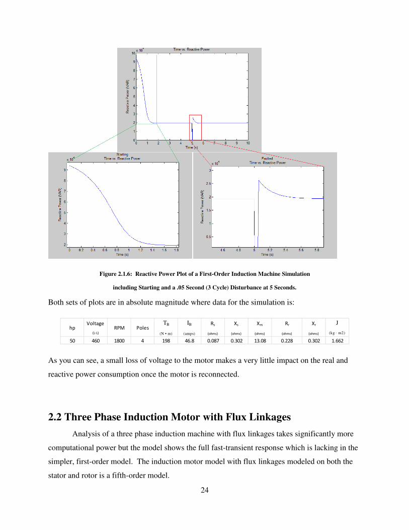
Below are first-order induction machine simulations showing motor starting, and a .05
second disturbance at 5 seconds. The top graph shows the entire 10 second simulation window
and the bottom tier focuses on starting (left) and faulted (right) conditions. The first picture set is
of real power and the second is of reactive power.
Figure 2.1.5: Real Power Plot of a First-Order Induction Machine Simulation including
Starting and a .05 Second (3 Cycle) Disturbance at 5 Seconds.
24
Figure 2.1.6: Reactive Power Plot of a First-Order Induction Machine Simulation
including Starting and a .05 Second (3 Cycle) Disturbance at 5 Seconds.
Both sets of plots are in absolute magnitude where data for the simulation is:
As you can see, a small loss of voltage to the motor makes a very little impact on the real and
reactive power consumption once the motor is reconnected.
2.2 Three Phase Induction Motor with Flux Linkages
Analysis of a three phase induction machine with flux linkages takes significantly more
computational power but the model shows the full fast-transient response which is lacking in the
simpler, first-order model. The induction motor model with flux linkages modeled on both the
stator and rotor is a fifth-order model.
hpVoltage
(L-L)
RPM PolesTB
(N • m)
IB
(amps)
Rs
(ohms)
Xs
(ohms)
Xm
(ohms)
Rr
(ohms)
Xr
(ohms)
J
(kg · m2)
50 460 1800 4 198 46.8 0.087 0.302 13.08 0.228 0.302 1.662

25
2.2.1 Voltage Equations in Machine Variables
The general voltage equations for a 3-phase induction machine may be expressed by the
follow set of equations:
5+- = 3-:+- + Ht+-H9
5O- = 3-:O- + HtO-H9
5/- = 3-:/- + Ht/-H9
5+A = 3A:+A + Ht+AH9
5OA = 3A:OA + HtOAH9
5/A = 3A:/A + Ht/AH9
These equations can be written in matrix form as shown below [38]. (The s subscript denotes
variables associated with the stator windings and the r subscript denotes variables associated
with the rotor windings. The operator d/dt is written as p.)
u+O/- = v-w+O/- + �x+O/- u+O/A = vAw+O/A + �x+O/A
The winding resistances for the stator and rotor can now be expressed as the following 3x3
matrices.
v- = y3- 0 00 3- 00 0 3-z vA = y3A 0 00 3A 00 0 3Az
26
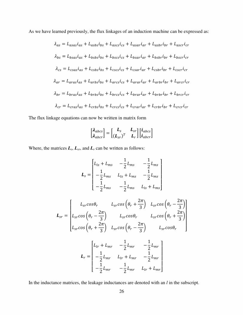
As we have learned previously, the flux linkages of an induction machine can be expressed as:
t+- = {+-+-:+- + {+-O-:O- + {+-/-:/- + {+-+A:+A + {+-OA:OA + {+-/A:/A
tO- = {O-+-:+- + {O-O-:O- + {O-/-:/- + {O-+A:+A + {O-OA:OA + {O-/A:/A
t/- = {/-+-:+- + {/-O-:O- + {/-/-:/- + {/-+A:+A + {/-OA:OA + {/-/A:/A
t+A = {+A+-:+- + {+AO-:O- + {+A/-:/- + {+A+A:+A + {+AOA:OA + {+A/A:/A
tOA = {OA+-:+- + {OAO-:O- + {OA/-:/- + {OA+A:+A + {OAOA:OA + {OA/A:/A
t/A = {/A+-:+- + {/AO-:O- + {/A/-:/- + {/A+A:+A + {/AOA:OA + {/A/A:/A
The flux linkage equations can now be written in matrix form
Fx+O/-x+O/AI = F |- |-A)|-A*b |A I Fw+O/-w+O/AI Where, the matrices Ls, Lsr, and Lr can be written as follows:
|- =}~~~~�{�- + {>- −12{>- −12{>-−12{>- {�- + {>- −12{>-−12{>- −12{>- {�- + {>-���
���
|-A =}~~~~� {-AK6;�A {-AK6; r�A + 2E3 s {-AK6; r�A − 2E3 s{-AK6; r�A − 2E3 s {-AK6;�A {-AK6; r�A + 2E3 s{-AK6; r�A + 2E3 s {-AK6; r�A − 2E3 s {-AK6;�A ��
����
|A =}~~~~�{�A + {>A −12{>A −12{>A−12{>A {�A + {>A −12{>A−12{>A −12{>A {�A + {>A���
���
In the inductance matrices, the leakage inductances are denoted with an l in the subscript.

27
It is convenient to refer the rotor variables to a winding with Ns turns (referred to stator).
w′+O/A = �A�- w+O/A
u′+O/A = �A�- u+O/A
x′+O/A = �A�- x+O/A
v′A = r�A�-s� vA
The flux linkage equations can be rewritten in matrix form as:
F x+O/-x′+O/AI = F |- |′-A)|′-A*b |′A I F w+O/-w′+O/AI Where the inductance matrices will be as follows:
{>- = �-�A {-A
|′-A = r�-�As |-A = }~~~~� {>-K6;�A {>-K6; r�A + 2E3 s {>-K6; r�A − 2E3 s{>-K6; r�A − 2E3 s {>-K6;�A {>-K6; r�A + 2E3 s{>-K6; r�A + 2E3 s {>-K6; r�A − 2E3 s {>-K6;�A ��
����
{′�A = r�-�As� {�A
{>- = r�-�As� {>A

28
|′A = r�-�As� |A = }~~~~�{′�A + {>- −12{>- −12{>-−12{>- {′�A + {>- −12{>-−12{>- −12{>- {′�A + {>-���
���
The voltage equations expressed in terms of machine variables referred by a turns-ratio to the
stator windings are:
u+O/- = v-w+O/- + �x+O/- u′+O/A = v′Aw′+O/A + �x′+O/A
In terms of inductances this becomes:
C u+O/-u′+O/AD = Fv- + �|- �|′-A�)|�-A*b v′A + �|′AI F w+O/-w′+O/AI Therefore, the voltages in the stator reference frame in matrix form are:
}~~~~�5+-5O-5/-5′+A5′OA5′/A ��
����= �
}~~~~� :+-:O-:/-:′+A:′OA:′/A ��
����
Where A is:
}~~~~~~~~~~~� 3- + �){�- + {>-* � r−12{>-s � r−12{>-s �{>-K6;�A �{>-K6; r�A + 2E3 s �{>-K6; r�A − 2E3 s� r−12{>-s 3- + �){�- + {>-* � r−12{>-s �{>-K6; r�A − 2E3 s �{>-K6;�A �{>-K6; r�A + 2E3 s� r−12{>-s � r−12{>-s 3- + �){�- + {>-* �{>-K6; r�A + 2E3 s �{>-K6; r�A − 2E3 s �{>-K6;�A
�{>-K6;�A �{>-K6; r�A − 2E3 s �{>-K6; r�A + 2E3 s 3′A + �){′�A + {>A* � r−12{>As � r−12{>As�{>-K6; r�A + 2E3 s �{>-K6;�A �{>-K6; r�A − 2E3 s � r−12{>As 3′A + �){′�A + {>A* � r−12{>As�{>-K6; r�A − 2E3 s �{>-K6; r�A + 2E3 s �{>-K6;�A � r−12{>As � r−12{>As 3′A + �){′�A + {>A*���
����������
2.2.2 Machine Equations in the Arbitrary Reference Frame

29
The complexity of the matrix above makes analysis in the stator reference frame difficult
and time consuming. To simplify the computations, we refer all variables to the arbitrary
reference frame with a reference velocity of synchronous velocity. In order to convert the
previously developed machine equations in the arbitrary reference frame, we must perform a
transformation of the variables to convert the varying inductances to a constant value. The
fundamentals of this transformation are defined as follows.
� k�- = �-�+O/- �+O/- = )�-*Y�� k�-
�- = 23}~~~~�cos � cos r� − 2E3 s cos r� + 2E3 ssin � sin r� − 2E3 s sin r� + 2E3 s12 12 12 ���
���
)�-*Y� = }~~~� cos � sin � 1cos r� − 2E3 s sin r� − 2E3 s 1cos r� + 2E3 s sin r� + 2E3 s 1���
��
�′ k�A = �A�′+O/A
�′+O/A = )�A*Y��′ k�A
�A = 23}~~~~�cos)� − �A* cos r� − �A − 2E3 s cos r� − �A + 2E3 ssin)� − �A* sin r� − �A − 2E3 s sin r� − �A + 2E3 s12 12 12 ���
���
)�A*Y� =}~~~� cos)� − �A* sin)� − �A* 1cos r� − �A − 2E3 s sin r� − �A − 2E3 s 1cos r� − �A + 2E3 s sin r� − �A + 2E3 s 1���
��

30
First, we will apply the fundamentals of transformation to the matrix equation for vabcs to convert
all the stator voltages and currents to arbitrary voltages and currents.
u+O/- = v-w+O/- + �x+O/- )�-*Y�u k�- = v-)�-*Y�w k�- + �n)�-*Y�x k�-o u k�- = �-v-)�-*Y�w k�- +�-�n)�-*Y�x k�-o
u k�- = �-v-)�-*Y�w k�- +�-�n)�-*Y�x k�-o + �-)�-*Y��x k�- u k�- = v-w k�- + B-xk - + �x k�-
Next, we will apply the fundamentals of transformation to the matrix equation for v’abcr.
u′+O/A = v′Aw′+O/A + �x′+O/A
)�A*Y�u′ k�A = v′A)�A*Y�w′ k�A + �n)�A*Y�x′ k�Ao u′ k�A = �Av′A)�A*Y�w′ k�A +�A�n)�A*Y�x′ k�Ao
u′ k�A = �Av′A)�A*Y�w′ k�A +�A�n)�A*Y�x′ k�Ao + �A)�A*Y��x′ k�A
u′ k�A = v′Aw′ k�A + )B- − BA*x′k A + �x′ k�A
Now that the stator voltages have been transformed to the rotor, we can rewrite the voltage
equation matrix as:
u k�- = v-w k�- + B-xk - + �x k�- u′ k�A = v′Aw′ k�A + )B- − BA*x′k A + �x′ k�A
Next, we must look at the matrix for λqd0s because it needs to be fully transformed. Again we
will apply the fundamentals of transformation to the components of λqd0s.
x+O/- = |-w+O/- + |′-Aw′ k�A
)�-*Y�x k�- = |-)�-*Y�w k�- + |′-A)�A*Y�w′ k�A

31
x k�- = �-|-)�-*Y�w k? +�-|′-A)�A*Y�w′ kA
�-|-)�-*Y� = y{�- + {> 0 00 {�- + {> 00 0 {�-z �-|′-A)�A*Y� = y{> 0 00 {> 00 0 0z
Next, we will fully transform the λ’qd0r matrix. We will once again apply the fundamentals of
transformation to the components of λ’qd0r.
x′ k�A = )|�-A*bw+O/- + |′Aw′ k�A
)�A*Y�x′ k�A = )|�-A*b)�-*Y�w k�- + |′A)�A*Y�w′ k�A
x′ k�A = �A)|�-A*b)�-*Y�w k�- +�A|′A)�A*Y�w′ k�A
�A)|�-A*b)�-*Y� = y{> 0 00 {> 00 0 0z �A|′A)�A*Y� = �{′�A + {> 0 00 {′�A + {> 00 0 {′�A�
Where,
{> = 32{>- Now the transformation is complete, we can write useful equations in matrix form.
� x k�-x′ k�A� = F �-|-)�-*Y� �-|′-A)�A*Y��A)|�-A*b)�-*Y� �A|′A)�A*Y� I � w k�-w′ k�A� The new matrix equations for flux linkages in the rotor reference frame can be expanded as
shown.

32
}~~~~~� t -tk-t�-t′ At′kAt′�A��
����� =
}~~~~�{�- + {> 0 0 {> 0 00 {�- + {> 0 0 {> 00 0 {�- 0 0 0{> 0 0 {′�A + {> 0 00 {> 0 0 {′�A + {> 00 0 0 0 0 {′�A��
����
}~~~~~� : -:k-:�-:′ A:′kA:′�A���
����
In addition to the flux linkage equations, we can write the new voltage equations in matrix form.
u k�- = v-w k�- + B-xk - + �x k�- u′ k�A = v′Aw′ k�A + )B- − BA*x′k A + �x′ k�A
}~~~~� 5 -5k-5?-5′ A5′kA5′�A��
����=}~~~~~�3- + �){�- + {>* B-){�- + {>* 0 �{> B-{> 0−B-){�- + {>* 3- + �){�- + {>* 0 −B-{> �{> 00 0 3- + �{�- 0 0 0�{> )B- − BA*{> 0 3′A + �){′�A + {>* )B- −BA*){′�A + {>* 0−)B- −BA*{> �{>k 0 −)B- − BA*){′�A + {>* 3′A + �){′�A + {>* 00 0 0 0 0 3′A + �{��A���
����
}~~~~~� : -:k-:�-:′ A:′kA:′�A���
����
As we can see, the matrix associated with the arbitrary reference frame is much easier to work
with than that associated with the stator reference frame.
Below are first-order induction machine simulations showing motor starting, and a .05
second disturbance at 5 seconds. The top graph shows the entire 10 second simulation window
and the bottom tier focuses on starting (left) and faulted (right) conditions. The first picture set is
of real power and the second is of reactive power.

33
Figure 2.2.2.1: Real Power Plot of a Fifth-Order Induction Machine Simulation including Starting and a .05 Second (3 Cycle) Disturbance at 5 Seconds.
Figure 2.2.2.2: Reactive Power Plot of a Fifth-Order Induction Machine Simulation including Starting and a .05 Second (3 Cycle) Disturbance at 5 Seconds.

34
Both sets of plots are in absolute magnitude where data for the simulation is:
As you can see a short loss of voltage to the motor creates a large fast-transient on the real and
reactive power once the motor is reconnected.
2.3 Induction Machine Modeling for Stability Analysis
The induction machine model used for stability analysis is a third-order model that
combines the simplicity of the basic induction machine model but also includes rotor flux
linkages, while ignoring stator flux linkages [3]. All parameters used in the equations in this
model are in per-unit. This allows the induction machine load to be placed on a transmission
level bus where in reality, induction motors are typically made for voltages of 4000V, 2300V,
460V or lower [12]. Distribution voltages are very rarely represented in a model of a particular
power system due to the massive amount of buses that would need to be included. The induction
motor model for stability analysis has been around for some time, however, stability analysis has
evolved from multivariable Nyquist criterion and eigenvalue analysis, to oscillation and voltage
studies [15] [16] [17]. The equations for the induction motor for stability analysis are:
H4′kH9 = r 1�′?s �−4�k + )e − e�*: � + )BA −B-*4′
H4′ H9 = r 1�′?s �−4� − )e − e�*:k� − )BA −B-*4′k
where,
e = e� + e>
e′ = e� + e>e�e> + e�
�′? = e� + e>B-�A
hpVoltage
(L-L)
RPM PolesTB
(N • m)
IB
(amps)
Rs
(ohms)
Xs
(ohms)
Xm
(ohms)
Rr
(ohms)
Xr
(ohms)
J
(kg · m^2)
50 460 1800 4 198 46.8 0.087 0.302 13.08 0.228 0.302 1.662

35
The term �′? is the transient open-circuit time constant that can be expressed in radians or
seconds. When the stator is open-circuited, this term characterizes the decay of rotor transients.
Equations for rotor speed, electrical torque, and mechanical torque must be expressed in per-unit
quantities, although, they are similar to both the first and fifth-order models.
HBAH9 = �B-2L� )�2�2/ − ��* �2�2/ = �4′k:k + 4′ : �B- , �� = �'?>)NBA� + pBA + q*
Figure 2.3.1: Real Power Plot of a Fifth-Order Induction Machine Simulation including Starting and a .05 Second (3 Cycle) Disturbance at 5 Seconds.

36
Figure 2.3.2: Reactive Power Plot of a Fifth-Order Induction Machine Simulation including Starting and a .05 Second (3 Cycle) Disturbance at 5 Seconds.
Both sets of plots are in per-unit where data for the simulation is:
As you can see a short loss of voltage to the motor creates a large fast-transient on the real and
reactive power once the motor is reconnected.
Rs
(ohms)
Xs
(ohms)
Xm
(ohms)
Rr
(ohms)
Xr
(ohms)
H
(s)
0.0068 0.1105 3.4895 0.0178 0.0605 1.2

37
Chapter 3: Optimization Algorithms
There are many algorithms and mathematical tools that can be used to solve various
optimization problems; considering deviations or tools, methods, and combinations, the
possibilities are endless. Increases in processing power also facilitate the use of algorithms that
once were considered computationally cumbersome.
Figure 3.1: Classification of Global Optimization Techniques [39].
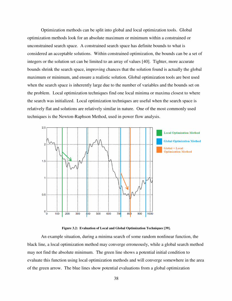
Optimization methods can
optimization methods look for an absolute
unconstrained search space. A constrained search space has definite bounds to what
considered an acceptable solutions.
integers or the solution set can be limited to an array of values
bounds shrink the search space, improving chances that
maximum or minimum, and ensure a
when the search space is inherently large due to the number of variables and the bounds set on
the problem. Local optimization
the search was initialized. Local optimization techniques are useful when the search space is
relatively flat and solutions are relatively similar in nature. One of the most commonly used
techniques is the Newton-Raphson Method, used in power flow analy
Figure 3.2: Evaluation of Local and Global Optimization Techniques
An example situation, during a minima search of some random nonlinear function, the
black line, a local optimization method may converge erroneou
may not find the absolute minimum
evaluate this function using local optimization methods
of the green arrow. The blue lines show potential evaluations from a global optimization
38
Optimization methods can be split into global and local optimization tool
imization methods look for an absolute maximum or minimum within a constrained or
. A constrained search space has definite bounds to what
acceptable solutions. Within constrained optimization, the bounds can be
or the solution set can be limited to an array of values [40]. Tighter, more accurate
improving chances that the solution found is actually the global
ensure a realistic solution. Global optimization tools are best used
when the search space is inherently large due to the number of variables and the bounds set on
the problem. Local optimization techniques find one local minima or maxima closest to where
Local optimization techniques are useful when the search space is
relatively flat and solutions are relatively similar in nature. One of the most commonly used
Raphson Method, used in power flow analysis.
: Evaluation of Local and Global Optimization Techniques [39].
An example situation, during a minima search of some random nonlinear function, the
black line, a local optimization method may converge erroneously, while a global search method
may not find the absolute minimum. The green line shows a potential initial condition to
using local optimization methods and will converge somewhere in the area
of the green arrow. The blue lines show potential evaluations from a global optimization
split into global and local optimization tools. Global
a constrained or
. A constrained search space has definite bounds to what is
the bounds can be a set of
Tighter, more accurate
solution found is actually the global
Global optimization tools are best used
when the search space is inherently large due to the number of variables and the bounds set on
closest to where
Local optimization techniques are useful when the search space is
relatively flat and solutions are relatively similar in nature. One of the most commonly used
An example situation, during a minima search of some random nonlinear function, the
, while a global search method
. The green line shows a potential initial condition to
and will converge somewhere in the area
of the green arrow. The blue lines show potential evaluations from a global optimization

39
method, none of which are actually a global or local minimum. Combining global and local
optimization techniques will yield the best possible outcome. Beginning with a global search
algorithm, the function will be evaluated and the best global value be used as the initial condition
for the local optimization method. In this case for finding the global minimum, the best result
from the blue lines is used as the initial condition for the orange arrow. This results in the actual
global minimum, the orange line, being the final output.
The two optimization algorithms used are the genetic algorithm (GA) and constrained
multivariable function minimization. The genetic algorithm is a global optimization method that
was developed from biological evolution.
3.1 The Genetic Algorithm
Genetic algorithms mimic cellular biology through chromosomal division. An individual
chromosome is a singular solution set to a problem, and many chromosomes make up a
population. Chromosomes may also be called ‘individuals’ in a population set.
Figure 3.1.1: Populations are Made Up Chromosomes, the Possible Solutions for the Problem [41].
A particular population set is considered a generation. Successive generations acquire a new
population set through selection, crossover, and mutation. The current generation is called the
parent generation and the next is called the child generation. For the genetic algorithm this cycle
continues until some stopping criteria is met.

The genetic algorithm process is best described by:
Figure 3.1.2: Structure of the Genetic Algorithm Implementation
The genetic algorithm is initialized
crossover and mutation rates and options, and stopping criteria.
Selection options are stochastic uniform, remainder, uniform, roulette, and tournamen
Each option varies in how the parents
uniform algorithm assigns each parent a
uniform steps through the set, where the first step is a
pair the parents together [40]. The parents then produce a child through crossover or mutation.
This method ensures that the diversity of individuals stays high and search space is ad
covered. Diversity is the average distance between individuals in a population.
such as tournament select the fittest
Tournament selection can lead to low diversity resulti
being unexplored.
Elite counts are simply the number of elite children that are selected to continue to the
next generation without changing
individuals/chromosomes undergo no mutation or crossover during reproduction.
40
The genetic algorithm process is best described by:
: Structure of the Genetic Algorithm Implementation [42].
The genetic algorithm is initialized by setting population size, selection options, elite counts,
crossover and mutation rates and options, and stopping criteria.
Selection options are stochastic uniform, remainder, uniform, roulette, and tournamen
Each option varies in how the parents (set of two chromosomes) are paired together. Stochastic
assigns each parent a consecutive number (e.g. 1, 2, 3, 4, 5, 6, …) and makes
, where the first step is a random number less than the step size, to
. The parents then produce a child through crossover or mutation.
This method ensures that the diversity of individuals stays high and search space is ad
Diversity is the average distance between individuals in a population.
fittest individual between pairs to breed the strongest
Tournament selection can lead to low diversity resulting in a vast portion of the search space
Elite counts are simply the number of elite children that are selected to continue to the
without changing. If the elite count is set to 4, then the 4 best
undergo no mutation or crossover during reproduction.
selection options, elite counts,
Selection options are stochastic uniform, remainder, uniform, roulette, and tournament.
are paired together. Stochastic
. 1, 2, 3, 4, 5, 6, …) and makes
random number less than the step size, to
. The parents then produce a child through crossover or mutation.
This method ensures that the diversity of individuals stays high and search space is adequately
Diversity is the average distance between individuals in a population. Other methods
between pairs to breed the strongest children.
ng in a vast portion of the search space
Elite counts are simply the number of elite children that are selected to continue to the
undergo no mutation or crossover during reproduction.

41
Crossover and mutation rates are percentages of the population that undergo crossover or
mutation. For example, if the population size 204 and the elite count is 4, there are 200 other
individuals they are matched through selection and crossover or undergo mutation. If the
crossover rate is .8, then 80% of the remaining population is matched through selected and
undergoes crossover )200 ∗ .8 = 160* thus the mutation rate must be .2, or 20%, and the
remaining individuals )200 ∗ .2 = 40* undergo mutation. Crossover options are typically
single-point, two-point, or multi-point.
Figure 3.1.3: Examples of Single-Point, Two-Point, or Multi-Point Crossover [41].
Likewise, mutation options are single-point, two-point, or multi-point.
Figure 3.1.4: Examples of Single-Point, Group, or Multi-Point Mutation [41].
Each generation is evaluated by the fitness function (function being minimized or
maximized) until stopping criteria is met. Stopping criteria can be generation limit, time limit,
fitness limit, stall generations, etc. If the stopping criterion is not met, then the genetic cycle
continues and a new generation is formed.
The base genetic algorithm works by minimizing a function, called a fitness function and
can be described mathematically by:
min� �)�*;8Kℎ9ℎG9 � N ∙ � ≤ �N2 ∙ � = �2 7� ≤ � ≤ 8��

42
Where 7� and 8� are the lower and upper bounds of the search space, respectively. In this
formulation we assume that none of the constraints are nonlinear.
The genetic algorithm stochastically evaluates the search space to find a global minimum
but may not converge to the absolute minimum in that area.
3.2 Constrained Multivariable Function Minimization
As with global optimization, there are many local optimization tools and methods
available. The multivariable function minimization techniques can be used for any convex
optimization problem. The local optimization method used is the barrier method subset within
the interior-point algorithm. The problem can be staged as:
min� �)�*;8Kℎ9ℎG9 � N ∙ � ≤ � → U)�* ≤ 0N2 ∙ � = �2 → ℎ)�* = 07� ≤ � ≤ 8� � and transformed into a barrier point problem for > 0 resulting in [43],
min�,- �¢)�, ;* = min�,- �)�* − £ln);#*#
such that, ℎ)�* = 0, U#)�* + ;# = 0, ;# > 0
As decreases, �¢should approach the minimum of�)�*. For a direct step in (x,s) direction, the
Karush-Kuhn-Trucker (KKT) equations are solved via linear approximation resulting in the
Hessian of the Lagrangian of �¢. The Lagrangian function,{)�, t*, used by the KKT conditions
is: {)�, t* = �)�* +£t¥,#U#)�* +£t¦,#ℎ#)�*
resulting in the Hessian, L,
L = ∇��)�* +£t#∇�U#)�* +£t ∇�ℎ )�*¨#
The direct step (∆x,∆s) can then be calculated by solving the KKT conditions by a linearized
Lagrangian from,

43
}~~�L 00 SΛ M¦b M¥b0 −SM¦ 0M¥ −S 00 ���
� ª Δ�Δ;−Δt¦−Δt¥¬ = − }~~�∇� − M¦bt¦ − M¥bt¥St¥ − 4ℎU + ; ��
�� where,
M¥ = MGK6�:G,6�9ℎ4:,4�8G7:9VK6,;93G:,9�8,K9:6,, UM¦ = MGK6�:G,6�9ℎ44�8G7:9VK6,;93G:,9�8,K9:6,, ℎS = H:GU6,G76�;t¥ = {GU3G,U4<879:�7:4354K9636�UΛ = H:GU6,G76�tt¦ = {GU3G,U4<879:�7:4354K9636�ℎ4 = 6,4;54K9636�;:4U

44
Chapter 4: Load Modeling
The purpose of modeling is to replicate the power system as accurately as possible to
simulate present or potential scenarios on the actual power system. The level of detail expressed
in a model can vary on depending on the use and desired level of accuracy. Static simulations
such as power flow analysis, optimal power flow, contingency analysis, and short circuit analysis
give the simulator an idea of how the power system will behave at a steady-state operating point
[44]. Static simulations provide voltage, current, or bus voltage angle information for snapshot
in time. Dynamic modeling requires very detailed models to accurately simulate transients on
the power system. Dynamic models are used to model the time dependent behaviors of the
power system to evaluate angular and voltage stability.
Figure 4.1: Power System Components that Affect Voltage Stability [5].
There are many different programs used for power system simulation such as PSS/E,
PSLF, DSA Tools, PowerWorld, and PST (Power System Toolbox). Each program has varying

45
degrees of capabilities. For example, PSS/E and PSLF are the two main power system simulation
softwares for commercial use and are standalone software, while PST is primarily used for
research purposes and must be integrated with MATLAB. PSS/E is developed by Siemens and
primarily used on the east coast of the USA, whereas PSLF is developed by General Electric and
primarily used on the west coast.
4.1 Load Modeling in Software
The primary software used in this research was PSS/E. Both PST and DSA Tools were
explored and offer different advantages and disadvantages. PST is not considered open source
software but it is free to obtain and use. All of the modules in the toolbox are open, which means
the code is easy to view, verify, and follow, and PST is very easy to use. One drawback in PST
is that it does not calculate local bus frequency which is problematic for disturbance analysis.
DSA Tools, on the other hand, is very comprehensive, but somewhat more difficult to use. This
software is for commercial use, thus modeling equations are not readily available.
PSS/E was selected over DSA Tools as the simulation tool of choice due to PSS/E
popularity on the east coast of the United States. A sample simulation will be provided in a later
section to show differences between PSS/E and DSA Tools using the same set of models.
4.1.1 Models in PSS/E
Although there is currently a PSS/E version 33.0 released by Siemens, PSS/E version
32.0 is the version available to work with at Virginia Tech. Version 32.0 has static models,
LDFRBL, IEEELBL, induction motor models, CIMWBL, CIM5BL, CIM6BL, and a complex
CLODBL [45]. These models are used as bus load models indicated by the BL suffix. The
LDFRBL model is a constant power, constant current, load model with frequency sensitivity
given by:
� = �� r BB�s>� = �� r BB�s'� = �� r BB�sA
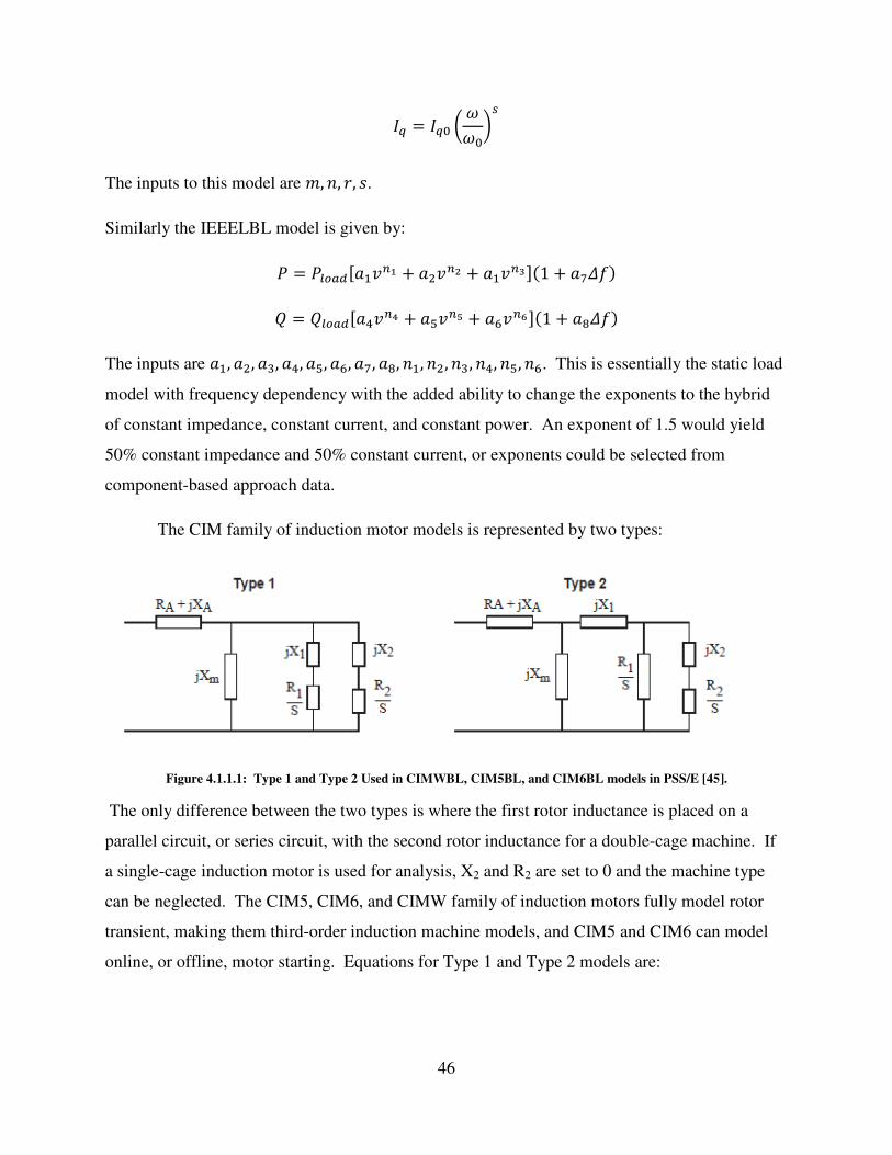
46
= � r BB�s- The inputs to this model are <, ,, 3, ;.
Similarly the IEEELBL model is given by:
� = ��?+k�G�5'® + G�5'¯ + G�5'°�)1 + G±��* � = ��?+k�G(5'² + G³5'´ + GZ5'µ�)1 + G¶��*
The inputs are G�, G�, G�, G(, G³, GZ, G±, G¶, ,�, ,�, ,�, ,(, ,³, ,Z. This is essentially the static load
model with frequency dependency with the added ability to change the exponents to the hybrid
of constant impedance, constant current, and constant power. An exponent of 1.5 would yield
50% constant impedance and 50% constant current, or exponents could be selected from
component-based approach data.
The CIM family of induction motor models is represented by two types:
Figure 4.1.1.1: Type 1 and Type 2 Used in CIMWBL, CIM5BL, and CIM6BL models in PSS/E [45].
The only difference between the two types is where the first rotor inductance is placed on a
parallel circuit, or series circuit, with the second rotor inductance for a double-cage machine. If
a single-cage induction motor is used for analysis, X2 and R2 are set to 0 and the machine type
can be neglected. The CIM5, CIM6, and CIMW family of induction motors fully model rotor
transient, making them third-order induction machine models, and CIM5 and CIM6 can model
online, or offline, motor starting. Equations for Type 1 and Type 2 models are:

47
Figure 4.1.1.2: Model Equations for Induction Motor Types 1 and 2 in PSS/E [46].
These single-cage equations are also given in the third-order induction machine section in
chapter 2. The CIMW model was made to adhere and be compatible with the WSCC Stability
Program induction machine model and cannot be used for motor starting studies. The other main
difference between the two models is the load torque equations used. The CIM5 model uses a
torque equation given by:
48
��?+k = �'?>)1 + ·B*¸
The CIM6 and CIMW models use a torque equation given by:
��?+k = �'?>,�)NB� + pB + q� + ·B�$* where,
q� = 1 − NB�� − pB� − ·B�$
B� = 1 + ∆B�
These two models use the more conventional torque equation where Tnom is the initialized load
torque, ω is the motor speed, ω0 is the initial motor speed and ∆ω0 is the motor’s deviation from
synchronous in per-unit slip. Tnom is initialized by setting the polynomial component equal to
one during initialization.
In PSS/E, induction motors and their driven loads are not affected by rotor angle
dynamics, but are sensitive to frequency and voltage changes. Driven loads typically consume
power proportional to speed, meaning as motor speed increases, power consumption also
increases, and as motor speed decreases, power consumption also decreases. The increase and
decrease in real power consumption contributes to system damping
It should be noted that modeling of induction motors in PSS/E should be checked for
numeric stability prior to being added into the load during a dynamic simulation. Principal time
constants for synchronous generators are long with respect to inertia and electromagnetics, while
induction motors generally have time constants near the upper end of the 0 to 30 rad/sec
bandwidth in PSS/E. In PSS/E the transfer function for motor speed to electrical torque is:
∆, = 1·>º ∆�21 + �2L>·> � ;»
where, ·> = ¼�2¼, + ¼��¼,

49
The time constant governing speed change is: 2L>·>
During initialization or transients, shorter inertia time constants in induction motors can cause a
sharp increase, or decrease, in mechanical speed thus causing slip to adjust accordingly.
Changes in slip result in variation of the rotor resistance, A- , which could cause numeric
instability. Also during initialization, the bus voltage along with the equivalent electrical circuit
is used to calculate initial slip and reactive power consumption of the motor. The initial slip is
then used to calculate initial torque so that the motor is started in steady-state for all dynamic
simulations. To compensate for the difference in load reactive power and reactive power
consumption by the aggregate induction motor, a hidden shunt is placed at the load bus. This
shunt can be calculated by the following:
½ �¾ � + �¾>?@?A = �¿l-�?+k ∗ %�>?@?A½ = �¿l-�?+k ∗ %�>?@?A − �¾>?@?A�¾ �
Where ½ is the compensating shunt, �¾>?@?A is the steady-state motor reactive power, �¿l-�?+k
is the bus load reactive power, and %�>?@?A is the percentage of motor load at the bus (can also
be represented by %�>?@?A since percentage of motor load is typically based on real power
consumption), and �¾ � is the steady-state bus voltage.
The CLOD type model is a composite load model that contains models for large
induction motors, small induction motors, discharge lighting, transformer saturation, constant
MVA, and remaining load which is expressed as a variable static model for real power and
constant impedance for reactive power. These load components are connected through a
transformer and a feeder within the model to the rest of the power system.
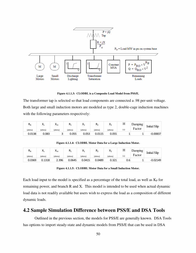
50
Figure 4.1.1.3: CLODBL is a Composite Load Model from PSS/E.
The transformer tap is selected so that load components are connected a .98 per-unit voltage.
Both large and small induction motors are modeled as type 2, double-cage induction machines
with the following parameters respectively:
Figure 4.1.1.4: CLODBL Motor Data for a Large Induction Motor.
Figure 4.1.1.5: CLODBL Motor Data for a Small Induction Motor.
Each load input to the model is specified as a percentage of the total load, as well as KP for
remaining power, and branch R and X. This model is intended to be used when actual dynamic
load data is not readily available but users wish to express the load as a composition of different
dynamic loads.
4.2 Sample Simulation Difference between PSS/E and DSA Tools
Outlined in the previous section, the models for PSS/E are generally known. DSA Tools
has options to import steady-state and dynamic models from PSS/E that can be used in DSA
RA
(ohms)
Xs
(ohms)
Xm
(ohms)
R1
(ohms)
X1
(ohms)
R2
(ohms)
X2
(ohms)
H
(s)
Damping
FactorInitial Slip
0.0138 0.083 3 0.055 0.053 0.0115 0.055 1 1 -0.00837
RA
(ohms)
Xs
(ohms)
Xm
(ohms)
R1
(ohms)
X1
(ohms)
R2
(ohms)
X2
(ohms)
H
(s)
Damping
FactorInitial Slip
0.0369 0.1318 2.396 0.0645 0.0415 0.0489 0.321 0.6 1 -0.02149

51
simulations by inputting the .raw and .dyr data files created in PSS/E. Using the exact same
models in both simulation programs, the results can vary slightly. Simulations were run in both
PSS/E and DSA Tools with a CIM5BL induction motor load with the following results:
Figure 4.2.1: Transient Voltage Comparison between PSS/E and DSA Tools.
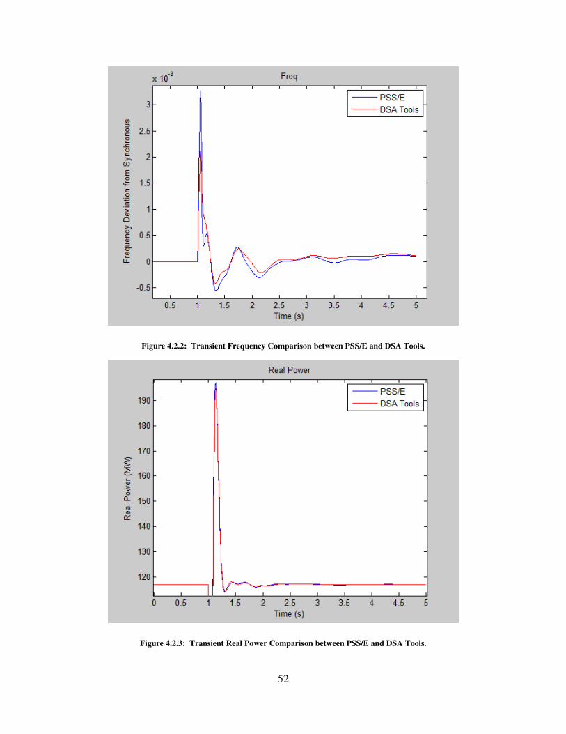
52
Figure 4.2.2: Transient Frequency Comparison between PSS/E and DSA Tools.
Figure 4.2.3: Transient Real Power Comparison between PSS/E and DSA Tools.

53
Figure 4.2.4: Transient Reactive Power Comparison between PSS/E and DSA Tools.
While the graphs of voltage, frequency, and real power are all relatively similar, the steady-state
conditions for reactive power are obviously different. The initial conditions for modeling
reactive power are the same in both PSS/E and DSA Tools, consisting of adding shunt
compensation [46] [47]. Both simulations use the same models and include a CIM5BL model at
the same bus with the data:
Figure 4.2.5: CIM5BL Induction Motor Data Used in Simulations for PSS/E and DSA Tools.
These differences show that modeling and simulation of the same scope can take different
approaches to perform calculations during a dynamic simulation.
RA
(ohms)
Xs
(ohms)
Xm
(ohms)
R1
(ohms)
X1
(ohms)
H
(s)
% Motor
Load
Damping
Factor
0.01 0.1105 2.6 0.018 0.0605 1.1 100 1

54
Chapter 5: Implementation of Optimization Algorithms for
Load Parameter Estimation
Simulations were done using the CIM6BL single-cage load model in PSS/E with a
variety of parameters and motor percentages to test how accurately the genetic algorithm and
constrained multivariable function minimization were able to match the parameters. Simulations
in PSS/E were performed by adding the motor load to an arbitrary load bus, bus number 110, and
applying a bus fault for .05 seconds or 3 cycles, then removing the fault. During simulation
time, frequency, voltage, real power, and reactive power were all recorded to be used in the
optimization algorithms. The inputs, frequency and voltage, were used to calculate real and
reactive power from the model in MATLAB.
Figure 5.1: Load Model Setup for Evaluation and Analysis within the Optimization Algorithms.
The WSCC 127 bus test system was used to collect simulated data to test the
implementation and testing of the combined genetic algorithm with the constrained,
multivariable function minimization where the function being minimization was the difference
between Real and Reactive Power in PSS/E and the MATLAB algorithm.
� �ÁÁ = ��ÂÂ/$ − �fÄb�Ä¿ �¸�ÁÁ = ��ÂÂ/$ − �fÄb�Ä¿
The fitness function for the genetic algorithm is:
min �)* = � �ÁÁ ∙ � �ÁÁb + �¸�ÁÁ ∙ �¸�ÁÁb

55
The chromosome for the genetic algorithm was representative of load parameters to be
used in optimization where the chromosome consisted of 17 elements:
= )�+, e+, e>, ��, e�, L, ��, N, p, �>?@?A , �>?@?A , ��, ��, ��, ��, ��, �� *
The first 11 parameters pertain to the induction motor where the circuit for the motor is,
Figure 5.2: Single-Cage Induction Motor Model used in Simulation.
Where H is the inertia constant, T0 is the starting torque, A and B are parameters of the torque
equation,
�� = �'?>)NBA� + pBA + q*
Åℎ434 �'?> :; KG7K87G94H ;8Kℎ 9ℎG9 )NBA� + pBA + q* = 1, and �>?@?A, and �>?@?A are the motor contributions to real and reactive power. The last 6
parameters pertain to the static ZIP model:
� �� = ������� � + ���� + ��� � �� = ������� � + ���� + ���
The optimization algorithms were set up such that:
min" �)* ;8Kℎ 9ℎG9 � N ∙ ≤ �N2 ∙ = �2 7� ≤ ≤ 8�� where,

56
N = 0, � = 0 N2 =
}~~~� 0 0 0 0 0 0 0 1 1 0 0 0 0 0 0 0 00 0 0 0 0 0 0 0 0 1 0 1 1 1 0 0 00 0 0 0 0 0 0 0 0 0 1 0 0 0 1 1 10 0 0 0 0 0 0 0 0 1 −1 0 0 0 0 0 00 0 0 0 0 0 1 0 0 0 0 0 0 0 0 0 0 ��
���,
�2 =}~~~�11101���
��
Where these correspond to,
N + p = 1 �>?@?A + �� + �� + �� = 1 �>?@?A + �� + �� + �� = 1 �>?@?A = �>?@?A �� = 1
The coefficients in the load torque equation must be equal to 1, the contributions from motor real
power plus static real power must be equal to the real power load, likewise, the contributions
from motor reactive power plus static reactive power must be equal to the reactive power load,
the percentage contribution of real power from a motor must be equal to the percentage
contribution of reactive power, and the initial torque was set to one as motor starting is not a
concern at this time.
The lower and upper bounds for optimization were generally left open from the various
motor parameter figures shown in Chapter 2. The bounds correspond to the chromosome :
= )�+, e+, e>, ��, e�, L, ��, N, p, �>?@?A , �>?@?A , ��, ��, ��, ��, ��, �� *
7� = �0.005, 0.05, 1.5, 0.005, 0.05,0.3,1,0,0,0,0,0,0,0,0,0,0� 8� = �0.1,0.2,4.5,0.1,0.25,3,1,1,1,1,1,1,1,1,1,1,1�
Expressed individually as:

57
0.005 ≤ �+ ≤ 0.1, 0.05 ≤ e+ ≤ 0.2, 1.5 ≤ e> ≤ 4.5, 0.005 ≤ �� ≤ 0.1,0.05 ≤ e� ≤ 0.25, 0.3 ≤ L ≤ 3, 1 ≤ �� ≤ 1, 0 ≤ N ≤ 1,0 ≤ p ≤ 1, 0 ≤ �>?@?A ≤ 1, 0 ≤ �>?@?A ≤ 1, 0 ≤ �� ≤ 1,0 ≤ �� ≤ 1, 0 ≤ �� ≤ 1, 0 ≤ �� ≤ 1, 0 ≤ �� ≤ 1, 0 ≤ �� ≤ 1 The initial chromosome was set as static load when evaluating motor load, and set as a large
portion of motor load when evaluating the static condition to show that the algorithm will
converge elsewhere. In practice this ‘guess’ should be used as a best estimate.
Parameters for the genetic algorithm were set to 350 for population size, 200 for
generations, 25 for stall generation (optimization would cease if the fitness function stopped
improving for 25 generations), and .7 for the crossover fraction. Two-point crossover was
selected as the crossover option to exchange data of the chromosomes at two points since the
latter half was primarily percentage based. Termination tolerances on constraints, on function
value, and on parameter values were set to 1·10-8
. Increasing the population size and/or
generations would result in better search area coverage per generation at the cost of time. The
crossover fraction was somewhat arbitrarily selected based on MATLAB recommendations
between .6 and .8 for optimum search space coverage. The number of elite children was left at
the default of 2 since the constrained multivariable function minimization was used to find the
local minima.
5.1 Results
A few different data sets were used to obtain data from PSS/E and were applied to the
optimization. The loads applied were static, 100% small motor, 100% large motor, 50% small
motor, a custom set of motor parameters at 100%, and a custom set of motor parameters at 30%.
The parameters are as follows:

58
Small Motor Parameters:
Large Motor Parameters:
Custom Motor Parameters:
The large and small motor parameter sets were taken from An Interim Dynamic Induction Motor
Model for Stability Studies in the WSCC [17].
Ra Xa Xm R1 X1 H A B
0.031 0.1 3.2 0.018 0.18 0.7 1 0
Ra Xa Xm R1 X1 H A B
0.013 0.067 3.8 0.009 0.17 1.5 1 0
Ra Xa Xm R1 X1 H A B
0.0068 0.1105 2.1 0.0178 0.0605 0.9 1 0

59
5.1.1 Static Load
The static model used was 100% constant current for real power and 100% constant
admittance for reactive power.
Figure 5.1.1.1: Genetic Algorithm Best Individual and Fitness Value for Each Generation of the Static Load.
This plot shows the end result of the genetic algorithm optimization. The top plot is the
best individual, or chromosome, where the numbers along the x-axis correspond to:
�+, e+, e>, ��, e�, L, ��, N, p, �>?@?A , �>?@?A , ��, ��, ��, ��, ��, ��
The static plot was started with 100% motor load, which corresponds to parameter 10,
representing �>?@?A, and parameter 11, representing �>?@?A, were initialized to 1. The plots with
heavy portions of motor load were initialized with a combination of ZIP parameters to ensure
that the algorithm to converge to an adequate solution. The bottom plot is of the best fitness
value and mean fitness value. Because the simulation was intentionally initialized with the
opposite composition parameters, the fitness value starts out very high and converges to a more
reasonable value. The best fitness value and mean fitness value is also labeled just above the
respective graph.

60
Figure 5.1.1.2: Reactive Power Plot of Optimization Output and PSS/E Output for the Static Load Simulation.
Figure 5.1.1.3: Real Power Plot of Optimization Output and PSS/E Output for the Static Load Simulation.
These two graphs that show how accurately the real and reactive power were matched between
simulation in PSS/E and the optimization’s output in MATLAB.

61
Optimization Output:
This output is taken after the constrained multivariable function minimization which may differ
from the genetic algorithm optimization.
Ra Xa Xm R1 X1 H To A B
0.0549 0.1404 3.0605 0.0338 0.1778 1.6917 1 0.5081 0.4919
Pmotor Qmotor p1 p2 p3 q1 q2 q3
0.0015 0.0015 0.8906 0.1051 0.0028 0.674 0.3109 0.0135

62
5.1.2 Small Motor Parameters at 100% Load
First Iteration:
Figure 5.1.2.1: Genetic Algorithm Best Individual and Fitness Value for Each Generation of the 100% Small Motor Load Simulation.
Figure 5.1.2.2: Reactive Power Plot of Optimization Output and PSS/E Output for 100% Small Motor Load Simulation.

63
Figure 5.1.2.3: Real Power Plot of Optimization Output and PSS/E Output for 100% Small Motor Load Simulation.
Optimization Output:
Ra Xa Xm R1 X1 H To A B
0.0417 0.1164 1.5112 0.039 0.1556 0.8307 1 0.8448 0.128
Pmotor Qmotor p1 p2 p3 q1 q2 q3
0.884 0.8897 0.038 0.0376 0.0419 0.0465 0.0477 0.0477

64
Second Iteration:
Figure 5.1.2.4: Genetic Algorithm Best Individual and Fitness Value for Each Generation of the 100% Small Motor Load Simulation.
Figure 5.1.2.5: Reactive Power Plot of Optimization Output and PSS/E Output for 100% Small Motor Load Simulation.
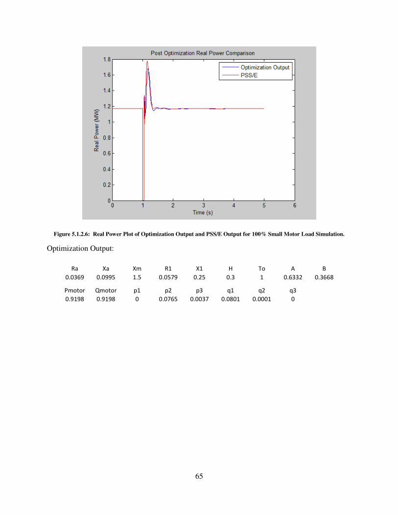
65
Figure 5.1.2.6: Real Power Plot of Optimization Output and PSS/E Output for 100% Small Motor Load Simulation.
Optimization Output:
Ra Xa Xm R1 X1 H To A B
0.0369 0.0995 1.5 0.0579 0.25 0.3 1 0.6332 0.3668
Pmotor Qmotor p1 p2 p3 q1 q2 q3
0.9198 0.9198 0 0.0765 0.0037 0.0801 0.0001 0

66
5.1.3 Large Motor Parameters at 100% Load
First Iteration:
Figure 5.1.3.1: Genetic Algorithm Best Individual and Fitness Value for Each Generation of the 100% Large Motor Load Simulation.
Figure 5.1.3.2: Reactive Power Plot of Optimization Output and PSS/E Output for 100% Large Motor Load Simulation.

67
Figure 5.1.3.3: Real Power Plot of Optimization Output and PSS/E Output for 100% Large Motor Load Simulation.
Optimization Output:
Ra Xa Xm R1 X1 H To A B
0.0385 0.05 1.5 0.0255 0.2207 0.8 1 1 0
Pmotor Qmotor p1 p2 p3 q1 q2 q3
0.8443 0.8443 0 0.1553 0.0003 0.1556 0 0

68
Second Iteration:
Figure 5.1.3.4: Genetic Algorithm Best Individual and Fitness Value for Each Generation of the 100% Large Motor Load Simulation.
Figure 5.1.3.5: Reactive Power Plot of Optimization Output and PSS/E Output for 100% Large Motor Load Simulation.

69
Figure 5.1.3.6: Real Power Plot of Optimization Output and PSS/E Output for 100% Large Motor Load Simulation.
Optimization Output:
Ra Xa Xm R1 X1 H To A B
0.0494 0.0897 1.5 0.0416 0.25 0.6 1 1 0
Pmotor Qmotor p1 p2 p3 q1 q2 q3
0.8857 0.8857 0 0.1122 0.0021 0.1142 0 0

70
5.1.4 Small Motor Parameters at 50% Load
First Iteration:
Figure 5.1.4.1: Genetic Algorithm Best Individual and Fitness Value for Each Generation of the 50% Small Motor Load Simulation.
Figure 5.1.4.2: Reactive Power Plot of Optimization Output and PSS/E Output for 50% Small Motor Load Simulation.
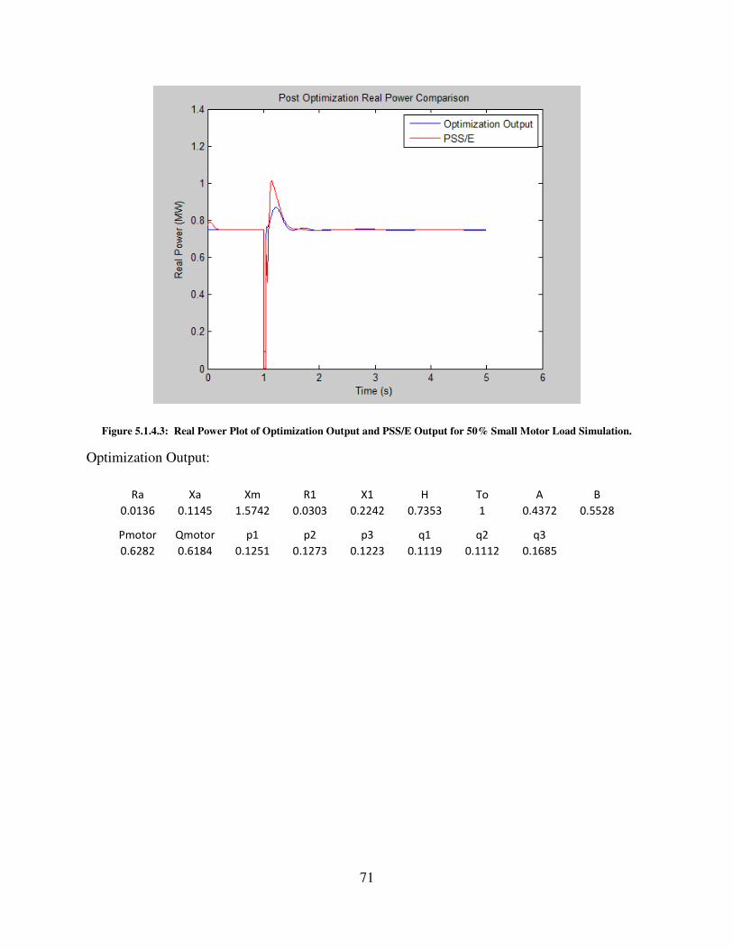
71
Figure 5.1.4.3: Real Power Plot of Optimization Output and PSS/E Output for 50% Small Motor Load Simulation.
Optimization Output:
Ra Xa Xm R1 X1 H To A B
0.0136 0.1145 1.5742 0.0303 0.2242 0.7353 1 0.4372 0.5528
Pmotor Qmotor p1 p2 p3 q1 q2 q3
0.6282 0.6184 0.1251 0.1273 0.1223 0.1119 0.1112 0.1685

72
Second Iteration:
Figure 5.1.4.4: Genetic Algorithm Best Individual and Fitness Value for Each Generation of the 50% Small Motor Load Simulation.
Figure 5.1.4.5: Reactive Power Plot of Optimization Output and PSS/E Output for 50% Small Motor Load Simulation.

73
Figure 5.1.4.6: Real Power Plot of Optimization Output and PSS/E Output for 50% Small Motor Load Simulation.
Optimization Output:
Ra Xa Xm R1 X1 H To A B
0.01 0.1321 3 0.02 0.15 1.2192 1 0 1
Pmotor Qmotor p1 p2 p3 q1 q2 q3
0.5504 0.5504 0.4496 0 0 0.4495 0.0001 0

74
5.1.5 Custom Motor Parameters at 100% Load
Figure 5.1.5.1: Genetic Algorithm Best Individual and Fitness Value for Each Generation of the 100% Custom Motor Load Simulation.
Figure 5.1.5.2: Reactive Power Plot of Optimization Output and PSS/E Output for 100% Custom Motor Load
Simulation.

75
Figure 5.1.5.3: Real Power Plot of Optimization Output and PSS/E Output for 100% Custom Motor Load Simulation.
Optimization Output:
Ra Xa Xm R1 X1 H To A B
0.0293 0.05 1.5 0.0946 0.2235 0.3 1 0 1
Pmotor Qmotor p1 p2 p3 q1 q2 q3
0.9131 0.9131 0 0.0778 0.0091 0.0869 0 0
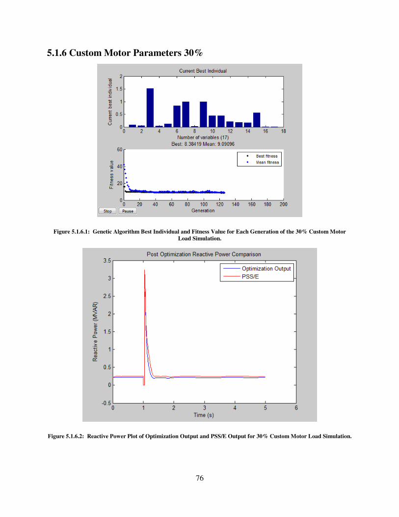
76
5.1.6 Custom Motor Parameters 30%
Figure 5.1.6.1: Genetic Algorithm Best Individual and Fitness Value for Each Generation of the 30% Custom Motor
Load Simulation.
Figure 5.1.6.2: Reactive Power Plot of Optimization Output and PSS/E Output for 30% Custom Motor Load Simulation.

77
Figure 5.1.6.3: Real Power Plot of Optimization Output and PSS/E Output for 30% Custom Motor Load Simulation.
Optimization Output:
Ra Xa Xm R1 X1 H To A B
0.085 0.051 1.5174 0.0362 0.1269 0.8388 1 0.0196 0.9902
Pmotor Qmotor p1 p2 p3 q1 q2 q3
0.4383 0.4472 0.2071 0.1878 0.172 0.5586 0.0014 0.0026

78
5.2 Discussion of Results
My simulation was effectively modeled and took measurements from an induction motor
connected to an infinite bus. In PSS/E, multi-machine dynamic equations are used to determine
how the entire system behaves under disturbance conditions. These equations are also used to
calculate voltage and frequency deviations. There is a discrepancy in real power calculations
between PSS/E and MATLAB due to a nearby generation in the PSS/E simulations. The
generator in PSS/E is two bus lengths away from the load bus where the fault was placed.
Shown in the equal area criterion section, the difference in power curves and operating point for
the generator cause a spike in power after the fault is removed from the system. This spike in
power by the generator is added to the post-disturbance real power consumption of the motor
alone.
The PSS/E simulation experiences a much higher level of damping due to the multi-
machine dynamics than the induction motor does when simulated on an infinite bus. The sharp
spike in the real power post disturbance with almost no oscillation post disturbance results in
lower motor inertia, H, and a shift in coefficients from A to B in the torque equation.
HBAH9 = r 12Ls )�2�2/ − ��*, HBAH9 = r 12Ls )�2�2/ − ��* = 0 G9 ;V,Kℎ36,68;
�2�2/ = �4′k:k + 4′ : �B- , �� = �'?>)NBA� + pBA + q*
Lowering H results in a greater speed deviation for the duration the fault persists, and a shift
from A to B in the torque equation results in synchronous torque at higher speed and for
rotational motion:
�6Å43 = �63�84 ∙ B
resulting in a higher spiking power while reducing post disturbance oscillations.
How PSS/E calculates its results is not explicitly known, nor are the model behaviors.
For example, machine equations must be calculated in the d-q reference frame and there are
many ways to use Park’s Transformation. The induction motor model used by PSS/E could be
some variation on the third-order induction machine model. Likewise, calculations for reactive

79
power are clearly different between PSS/E and DSA Tools. The model that is ‘most’ correct is
the one that takes assumptions one is willing to live with into consideration. It is impossible to
model every dynamic component or every aspect of the power system. Assumptions must be
made to lessen the computational burden of dynamic simulation.
Lastly, where can the bounds for the machine parameters be drawn? The limitation on
parameters in this work was strictly based on sets of possible induction machine parameters.
Should groups of parameters be lumped together (i.e. if the range for Ra is ‘x’ then Xa should be
within ‘y-z’ bounds?
The optimization algorithm does relatively well in estimating the percentage of motor
load during the disturbance. In almost all scenarios the optimization algorithm was able to
estimate motor load to within 15% of the actual percentage. In many cases, the algorithm was
able to place static load as constant current for real power, and constant admittance for reactive
power. In practice, static load is typically represented as 100% constant current for real power
and 100% constant impedance for reactive power.
5.3 Equal Area Criterion – Swinging of Synchronous Machines
The equal area criterion is used to analyze one machine’s swing with respect to an
infinite bus [48].
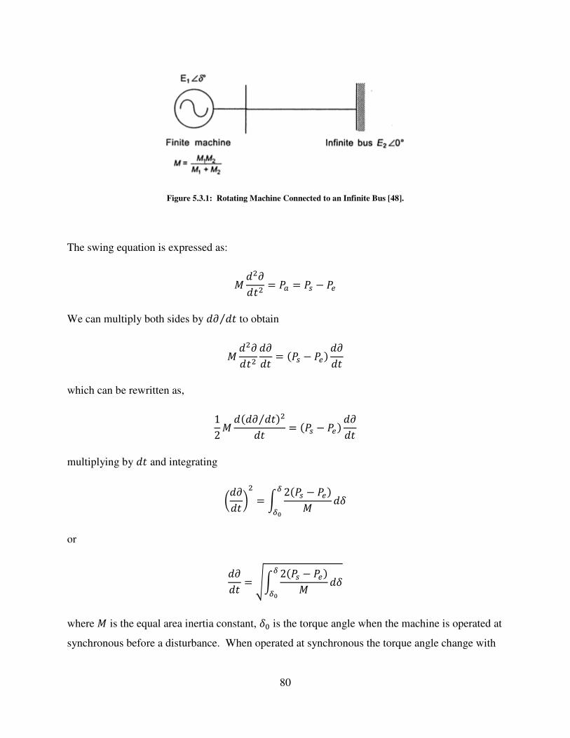
80
Figure 5.3.1: Rotating Machine Connected to an Infinite Bus [48].
The swing equation is expressed as:
= H�¼H9� = �+ = �- − �2
We can multiply both sides by H¼ H9⁄ to obtain
= H�¼H9� H¼H9 = )�- − �2* H¼H9
which can be rewritten as,
12 = H)H¼ H9⁄ *�H9 = )�- − �2* H¼H9
multiplying by H9 and integrating
rH¼H9 s� = Æ 2)�- − �2*=ÇÇÈ
HÉ
or
H¼H9 = ÊÆ 2)�- − �2*=ÇÇÈ
HÉ
where = is the equal area inertia constant, � is the torque angle when the machine is operated at
synchronous before a disturbance. When operated at synchronous the torque angle change with

81
respect to time is zero, H¼ H9⁄ = 0. Post disturbance the machine will operate again at
synchronous when:
Æ 2)�- − �2*=ÇÇÈ
HÉ = 0
However, the machine will not remain at synchronous during the first crossing of H¼ H9⁄ = 0.
This can be thought of as a pendulum on a rotating mass.
Figure 5.3.2: A Fixed-Point Pendulum and a Pendulum on a Rotating Mass [48].
Consider the pendulum attached to a fixed point as shown on the left. If the pendulum is
released slightly past point c, the pendulum will swing between points a and c until damping
brings the pendulum to rest at point b. Now consider a pendulum attached to a rotating mass.
As the pendulum moves from point c to point a, the combine angular velocity of the rotating
mass and pendulum is faster than that of the mass alone. Inversely, as the pendulum moves from
point a to point c, the combine angular velocity of the mass and pendulum is slower than that of
the mass alone. At points a and c the angular velocity is zero and the combined angular velocity
is equal to that of the mass. In this analogy, the angular velocity of the mass resembles the
synchronous speed of the motor and the pendulum represents the swinging of the motor with
respect to an infinite bus.
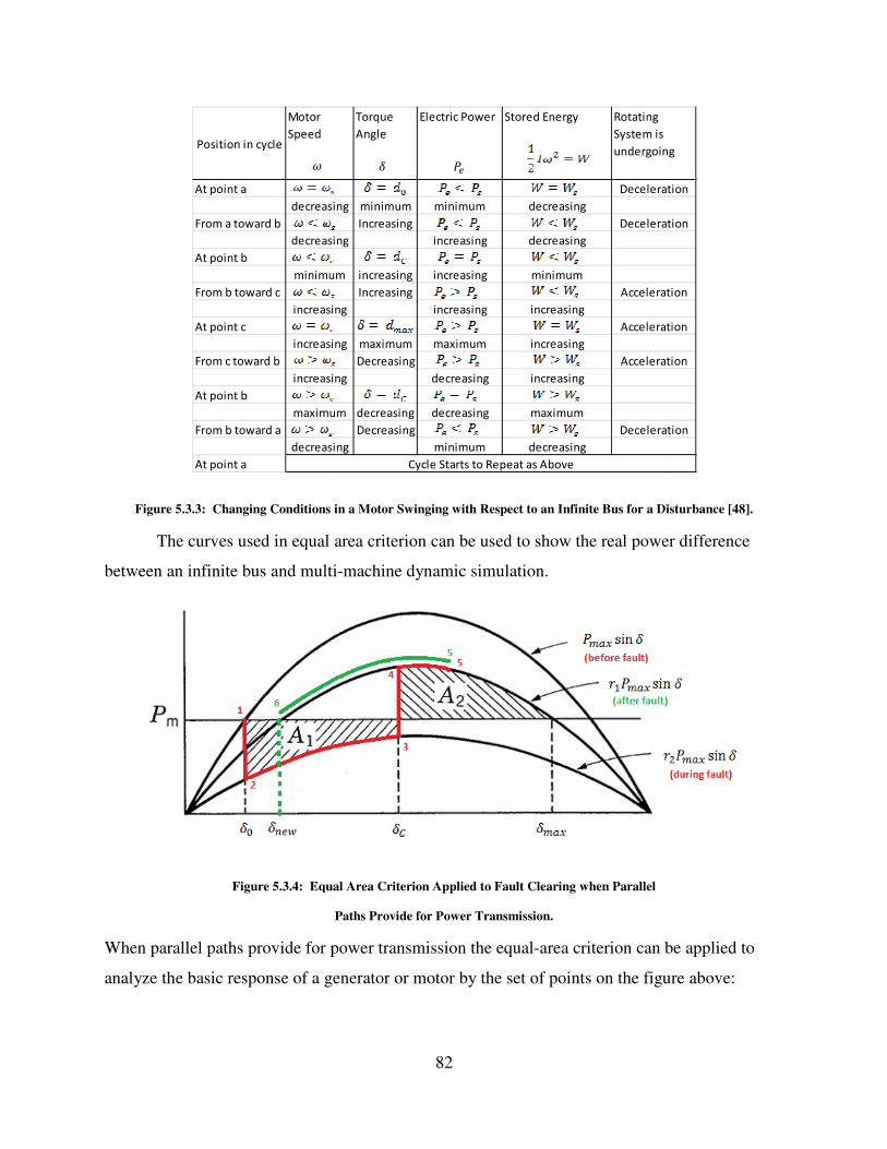
Figure 5.3.3: Changing Conditions in a Motor Swinging
The curves used in equal area criterion can be used to
between an infinite bus and multi
Figure 5.3.4: Equal
When parallel paths provide for power transmission the equal
analyze the basic response of a generator
Position in cycle
Motor
Speed
At point a
decreasing
From a toward b
decreasing
At point b
minimum
From b toward c
increasing
At point c
increasing
From c toward b
increasing
At point b
maximum
From b toward a
decreasing
At point a
B
82
: Changing Conditions in a Motor Swinging with Respect to an Infinite Bus for a Disturbance
equal area criterion can be used to show the real power difference
between an infinite bus and multi-machine dynamic simulation.
: Equal Area Criterion Applied to Fault Clearing when Parallel
Paths Provide for Power Transmission.
When parallel paths provide for power transmission the equal-area criterion can be applie
analyze the basic response of a generator or motor by the set of points on the figure above:
Torque
Angle
Electric Power Stored Energy Rotating
System is
undergoing
Deceleration
decreasing minimum minimum decreasing
Increasing Deceleration
decreasing increasing decreasing
minimum increasing increasing minimum
Increasing Acceleration
increasing increasing increasing
Acceleration
increasing maximum maximum increasing
Decreasing Acceleration
increasing decreasing increasing
maximum decreasing decreasing maximum
Decreasing Deceleration
decreasing minimum decreasing
Cycle Starts to Repeat as Above
�2É
with Respect to an Infinite Bus for a Disturbance [48].
show the real power difference
area criterion can be applied to
ints on the figure above:
System is
undergoing
Deceleration
Deceleration
Acceleration
Acceleration
Acceleration
Deceleration

83
1) The machine is initially operating somewhere on the É − � curve labeled (before fault)
prior to the fault.
2) Once a fault is placed on the system, the generator’s response is to speed up to attempt to
provide the power needed by the system, resulting in an increasing É.
3) The fault is cleared, restoring the generator’s ability to supply power, however the total
power needed is lessened due to other contributions on the system.
4) Inertia of the generator carries the generator past critical clearing angle, ÉË.
5) The generator begins to slow and the angle begins to decrease.
6) Although the generator will most likely oscillate around point 6 until settling at point 6,
the new operating point.
The spike in real power output from point 3 to point 4 explains lower measurement values in
MATLAB than seen in PSS/E.
In PSS/E, this effect can be seen by examining the bus voltage angle from a nearby
generator bus and the bus voltage angle of the load bus under study. The load bus under
investigation is 2 bus lengths away from the generator bus. When the fault is applied to the
system, the bus angle deviates from its initial value and begins to increase as the generator
speeds up. Post fault, the angles return somewhere nearby to their initial values. Although the
bus voltage angles may not return to their pre-fault values, the angle difference between the
nearby generator bus and the load bus undergoes a swing and the difference between the two
angles stabilizes.

84
Figure 5.3.5: Voltage Angle Deviation during a Fault as Related to the Equal Area Criterion.
Figure 5.3.6: Voltage Angle Difference Shows Stabilization between Load and Generator.
In practice, the bus angle would not change instantaneously with respect to time as this
represents an instantaneous change in velocity. The deviation in angle shows that power flows

85
from the generator to the load center under steady-state conditions, as it should. During the fault,
power flows in the reverse direction and upon clearing and reclosing the bus, the difference in
bus angles results in underdamped real power oscillations as the system returns to synchronism.

86
Chapter 6: Future Work
There are many possible options for continued work on load modeling with genetic
algorithms and constrained multivariable function minimization. The logical next step is to
benchmark the results obtained through optimization to actual measurements in the field. Real
data should be collected and used to obtain motor parameters, which should be inserted into
PSS/E to see if the simulation results match what happened in practice. Until real data can be
collected additional topics could be explored:
• How can the parameters be tuned to give a more accurate result?
• Can the genetic algorithm be written in python to run the comparative simulations in
PSS/E? This would provide the most accurate result, but would be the most
computationally intensive due to the volume of iterations needed by the GA.
• The model could be changed to the CMLDBL model which more accurately represents
different loads and replicate FIDVR (Section 6.2). This model allows for three 3-phase
motors, one 1-phase motor, electronic load, and static load. By separating the load into
three different motors, the parameters could be set to small and large motors where the
genetic algorithm could find percent contribution. This model is available in new
versions of PSS/E.
• Could PMU data prove more accurate when running the algorithm since voltage and
current phasors are measured? Instead of using voltage magnitude to convert Vabc into
the Vdq0 reference frame then calculating Idq, phasors would allow you to convert voltage
and current directly into the d-q reference frame.

87
6.1 Voltage Stability
Electric power is the last great commodity that can be considered a bargain in present
day.
Figure 6.1.1: Increase in Cost of Consumer Goods from 1985-2005 (Nominal Dollars) [49].
The power system will continue to be operated closer to stability limits to keep costs down as
investments in the grid are kept minimal. Operating closer to stability limits will require
accurate simulation to accurately represent voltage and angular stability to mitigate and prevent
outages. Transient voltage stability is often associated with transient rotor angle stability, while
longer duration voltage stability is interlinked with small-disturbance rotor angle stability [5].
Voltage stability is considered load stability, and rotor angle stability is considered generator
stability. Voltage collapse on a transmission point is most likely a result of an angle stability
issue, while voltage collapse in a load area is a voltage stability problem. Voltage collapse in
load areas is typically caused by stalling of motors. Critical voltage clearing points can be
calculated from the power transfer equations and normalized short circuit power by:
� = �eT� , � = �eT� , 5 = �T
based on the model,

Figure 6.1.2
Power transfer equations can be normalized as well,
� = T�� = T�
By using the trigonometric identity of
�6Å43 �GK963At unity power factor we can take the derivative and set it equal to 0, we can obtain the critical
voltage and maximum power.
H�H� = 0 = 125/A#@#/+� = 1√
Similarly we can use reactive power to calculate the Voltage Collapse Proximity Indicator
(VCPI) where:
� = 0, É = 0, �¥ = Í4,43G94H
H�H� = 0 = 1ewhich we can normalize as,
88
Figure 6.1.2: Circuit Used For Maximum Power Transfer.
Power transfer equations can be normalized as well,
T�e sin É , � = 5 sin É T� cos Ée − ��e , � = 5 cos É − 5�
By using the trigonometric identity of 5� sin� É + 5� cos� É = 5�:
�GK963 = g5� − 5� cos� É = g5� − )� + 5�*�
At unity power factor we can take the derivative and set it equal to 0, we can obtain the critical
)5� − 5(*Y� �⁄ )25 − 45�* ⟶ 25� = 1, 1√2 = .707, �>+� = g1 2⁄ − 1 4⁄ = 0.5
Similarly we can use reactive power to calculate the Voltage Collapse Proximity Indicator
Í4,43G94H 63 S4,H:,U T,H �, � = {6GH �4GK9:54� = T�e − ��e
)T − 2�*, �/A#@ = T2 , �>+� = ��e�?+k
At unity power factor we can take the derivative and set it equal to 0, we can obtain the critical
Similarly we can use reactive power to calculate the Voltage Collapse Proximity Indicator
�4GK9:54 �6Å43

89
5/A#@ = 0.5, �>+� = �>+�eT� = 0.25
and we can calculate the Voltage Collapse Proximity Indicator where,
�¥ = � + e� = � + e�¥�T� , �¥� − T�e �¥ + T�e � = 0
thus by the quadratic equation,
�¥ = 12 �T�e ± TÊT�e� − 4�e �
and we can calculate VCPI, kÑÒkÑ ,
H�¥H� = 1Ó1 − 4e�T�
= 1Ó1 − ��>+�
At a no load condition, � equals T, and at max load � equals T 2⁄ . This shows the voltage
collapse proximity indicator at a no load condition is unity and at a maximum load is infinity. At
maximum load, extremely large amounts of reactive power are required to support a small
increment in load.
6.2 Fault Induced Delayed Voltage Recovery (FIDVR)
As NERC continues to require increasing accuracy from power system operators, it is
critical to model key dynamic components for transient and voltage stability analysis.
Mentioned in TPL-001-2, requirements R2.4.1 and R5, planners will be required to model
dynamic loads for voltage stability analysis. While not explicitly stating the necessity to study
the effects of fault induced delayed voltage recovery (FIDVR) on power system operation, it is
certainly implied. FIDVR is a topic that has been under investigation for some time. Utilities in
the WECC have had more severe issues associated with voltage stability causing blackouts than
the east coast. Efforts within the WECC and by Bonneville Power Administration have yielded a

90
new composite load model, CMLDBL, which can accurately represent how FIDVR affects
voltage stability in simulation.
The CMLDBL allows for representation of 3 three-phase induction motors, 1 single-
phase induction motor, electronic load, and static load along with protection elements associated
with each. One of the primary differences in modeling protection elements in a model that can
accurately represent FIDVR is how the protection may actually operate in simulation. Static
models in PSS/E show voltage recovery almost instantaneously and model load using the CIM
family of induction motors does not result in delayed voltage recovery that would definitely trip
portions of the power system offline. However, during FIDVR conditions, the operation of
protection elements greatly affects the recovery of voltage and stability of the system. The
CMLDBL model was not available for study at Virginia Tech but could be used for future
parameter estimation. The use of three induction motors and one single phase motor would
facilitate better algorithm boundaries.

91
References
[1] G. W. Stagg and A. H. El-Abiad, Computer Mehtods in Power Systems, New York:
McGraw-Hill, 1968.
[2] J. D. Glover, M. S. Sarma and T. J. Overbye, Power System Analysis and Design, Cengage
Learning, 2008.
[3] P. Kundur, Power System Stability and Control, New York: McGraw-Hill, Inc., 1994.
[4] G. C. Bullock, "Cascading Voltage Collapse in West Tennessee," in 17th Annual Western
Protective Relay Conference, Spokane, Washington, 1987.
[5] C. W. Taylor, Power System Voltage Stability, New York: McGraw-Hill, Inc, 1994.
[6] Computer Analysis of Power Systems Working Group of the Computer and Analytical
Methods Subcommittee, "System Load Dynamics - Simulation Effects and Determination
of Load Constants," in IEEE PES Summer Meeting, San Francisco, 1972.
[7] Electric Machinery Committee, "IEEE Guide for Synchronous Generator Modeling
Practices and Applications in Power System Stability Analyses," IEEE Power Engineering
Society, New York, 2002.
[8] C. Concordia and S. Ihara, "Load Representation in Power Systems," IEEE Transactions on
Power Apparatus and Systems, Vols. PAS-101, no. No. 4, pp. 969-977, 1982.
[9] J. M. Undrill and T. F. Laskowski, "Model Selection and Data Assembly for Power System
Simulations," Power Technologies, Inc., Schenectady, New York, 1982.
[10] IEEE Task Force on Load Representation for Dynamic Performance, "Standard Load
Models for Power Flow and Dynamic Performance Simulation," IEEE Transactions on
Power Systems, vol. Vol. 10, no. No. 3, pp. 1302-1313, 1995.
[11] Siemens Power Technologies International, "Program Application Guide," Siemens
Energy, Inc., Schenectady, NY, 2009.
[12] IEEE Task Force on Load Representation for Dynamic Performance, "Load Representation
for Dynamic Performance Analysis," in IEEE Transactions on Power Systems, New York,
1993.

92
[13] IEEE Task Force on Load Representation for Dynamic Performance, "Bibliography on
Load Models for Power Flow and Dynamic Performance Simulation," IEEE Transactions
on Power Systems, vol. 10, no. 1, pp. 523-538, 1995.
[14] B. C. Lesieutre, P. W. Sauer and M. A. Pai, "Development and Comparative Study of
Induction Machine Based Dynamic P, Q Load Models," IEEE Transactions on Power
Systems, vol. 10, no. 1, pp. 182-191, 1995.
[15] R. Ueda and S. Takata, "Effects of Induction Machine Load on Power System," IEEE
Transactions on Power Apparatus and Systems, Vols. PAS-100, no. No. 5, 1981.
[16] K. R. Padiyar and P. Rajasekharam, "Effects of Induction Motor Load on Dynamic
Stability of Power Systems," Electric Machines and Power Systems, vol. 9, pp. 269-283,
1984.
[17] L. Pereira, D. Kosterev, P. Mackin, D. Davies, J. Undrill and W. Zhu, "An Interim
Dynamic Induction Motor Model for Stability Studies in the WSCC," IEEE Transactions
on Power Systems, vol. 17, no. 4, 2002.
[18] North American Electric Reliability Corporation, "Regional Entities," NERC, 2013.
[Online]. Available: http://www.nerc.com/AboutNERC/keyplayers/Pages/Regional-
Entities.aspx. [Accessed 15 May 2013].
[19] W. W. Price, K. A. Wirgau, A. Murdoch, J. V. Mitsche, E. Vaahedi and M. A. El-Kady,
"Load Modelling for Power Flow and Transient Stability Computer Studies," IEEE
Transactions on Power Systems, vol. 3, no. 1, pp. 180-187, 1988.
[20] D. Q. Ma and J. Ping, "A Novel Approach to Dynamic Load Modelling," IEEE
Transactions on Power Systems, vol. 4, no. 2, pp. 396-402, 1989.
[21] T. Dovan, T. S. Dillon, C. S. Berger and K. E. Forward, "A Microcomputer Based On-line
Identification Approach to Power System Dynamic Load Modelling," IEEE Transactions
on Power Systems, vol. 2, no. 3, pp. 529-536, 1987.
[22] C.-J. Lin, Y.-T. Chen, C.-Y. Chiou, C.-H. Huang, H.-D. Chiang, J.-C. Wang and L. Fekih-
Ahmed, "Dynamic Load Models in Power Systems Using the Measurement Approach,"
IEEE Transactions on Power Systems, vol. 8, no. 1, pp. 309-315, 1993.
[23] M. Sadeghi and G. A. Sarvi, "Determination of ZIP Parameters with Least Squares
Optimization Method," in IEEE Electrical Power & Energy Conference, 2009.

93
[24] F. J. Meyer and K. Y. Lee, "Dynamic Power System Load Modeling by Parameter
Estimation," Electric Power Systems Research, vol. 7, pp. 231-241, 1984.
[25] A. Prieto, "Artificial Neural Networks," in International Workshop on Artificial Neural
Networks, Granada, Spain, 1991.
[26] A. Goedtel, I. N. da Silva and P. J. A. Serni, "Load Torque Identification in Induction
Motor Using Neural Networks Technique," Electric Power Systems Research, vol. 77, pp.
35-45, 2007.
[27] M. Bostanci, J. Koplowitz and C. W. Taylor, "Identification of Power System Load
Dynamics Using Artificial Neural Networks," IEEE Transactions on Power Systems, vol.
12, no. 4, pp. 1468-1473, 1997.
[28] "DTREG - Software For Predictive Modeling and Forecasting," [Online]. Available:
http://www.dtreg.com/index.htm. [Accessed 17 May 2013].
[29] NERC, "Standard TPL-001-2 - Transmission System Planning Performance
Requirements," NERC Board of Trustees, 2011.
[30] University of Texas at Arlington, "Determining Load Characteristics for Transient
Performance," Electric Power Research Institute, 1979.
[31] General Electric Company, "Load Modelling for Power Flow and Transient Stability
Studies," Electric Power Research Institute, 1987.
[32] Ontario Hydro, "Extended Transient-Midterm Stability Program," Electric Power Research
Institute, 1985.
[33] T. Frantz, T. Gentile, S. Ihara, N. Simons and M. Waldron, "Load Behaviour Observed in
LLICO and RG&E Systems," IEEE Transactions on Power Systems, Vols. PAS-103, no. 4,
pp. 819-831, 1984.
[34] K. Srinivasan and R. Jutras, "Power System Disturance Monitoring System," in IEEE
Transmission & Distribution Conference, Dallas, 1991.
[35] S. J. Chapman, Electric Machinery and Power System Fundamentals, Boston: McGraw-
Hill, 2002.
[36] Anaheim Automation, "AC Motor Guide," Anaheim Automation, 2011. [Online].
Available: http://www.anaheimautomation.com/manuals/forms/ac-motor-guide.php.
[Accessed 20 May 2013].

94
[37] F. Nozari, M. D. Kankam and W. W. Price, "Aggregation of Induction Motors for Transient
Stability Load Modeling," IEEE Transctions on Power Systems, vol. 2, no. 4, pp. 1096-
1103, 1987.
[38] P. C. Krause and O. Wasynczuk, Electromechanical Motion Devices, New York: McGraw-
Hill Book Company, 1989.
[39] T. Weise, "Global Optimization Algorithms - Theory and Application -," 26 6 2009.
[Online]. Available: http://www.it-weise.de/projects/book.pdf. [Accessed 7 5 2013].
[40] MathWorks, "Documentation Center - Genetic Algorithm," MathWorks, 1994-2013.
[Online]. Available: http://www.mathworks.com/help/gads/genetic-algorithm.html.
[Accessed 22 May 2013].
[41] S. N. Sivanandam and S. N. Deepa, Introduction to Genetic Algorithms, Berlin: Springer,
2008.
[42] D. K. Chaturvedi, Soft Computing Techniques and its Applications in Electrical
Engineering,, Berlin: Springer-Verlag, 2008.
[43] MathWorks, "Optimization Toolbox," MathWorks, 1994-2013. [Online]. Available:
http://www.mathworks.com/help/optim/index.html. [Accessed 22 May 2013].
[44] L. L. Grigsby, Power System Stability and Control, Boca Raton: CRC Press, 2012.
[45] Power Technologies International, "Load Characteristic Models," in Program Application
Guide: Volume II, Siemens Energy, Inc., 2009, pp. 427-272.
[46] Power Technologies International, "Load Characteristic Model Data Sheets," in MODELS,
Siemens Energy, Inc., 2009, pp. 385-402.
[47] Powertech Labs, Inc., "Model Manual," in TSAT - Transient Security Assessment Tool,
Surrey, British Columbia, DSA Tools, 2010.
[48] W. D. Stevenson, Elements of Power System Analysis, Tokyo: McGraw-Hill, 1975.
[49] Edison Electric Institute, "Edison Electric Institute," May 2006. [Online]. Available:
http://www.eei.org/whatwedo/PublicPolicyAdvocacy/StateRegulation/Documents/rising_el
ectricity_costs.pdf. [Accessed 26 May 2013].

95
Appendix A – MATLAB Code:
%%%%%%%%%%%%%%%%%%%%%%%%%%%%%%%%%%%%%%%%%%%%%%%%%%%%%%%%%%%%%%%%%%%%%%%%%%% %%%% Utilizing Genetic Algorithms to Find Load Model Parameters %%%% Christopher Mertz %%%% Copyright 2013 %%%% Main %%%% Mertz_GAParameters3.m %%%%%%%%%%%%%%%%%%%%%%%%%%%%%%%%%%%%%%%%%%%%%%%%%%%%%%%%%%%%%%%%%%%%%%%%%%%
clc clear all close all
% %%% Import PSSE File %%%% [time, chan1, chan2, chan3, chan4] = PSSEData('THESISStaticSim.txt');
%%steady state voltage, Load P, Load Q sysbase = 100; ssvolt = chan2(60); Po = chan3(60); Qo = chan4(60);
%vars. 1 2 3 4 5 6 7 8 9 10 % [R1, X1, Xm, R2, X2, H, To, A, B, Pmotor, % Qmotor, p1, p2, p3, q1, q2, q3] %variables lb = [.005 .05 1.5 .005 .05 .3 1 0 0 0 ... 0 0 0 0 0 0 0]; ub = [.1 .2 4.5 .1 .25 3 1 1 1 1 ... 1 1 1 1 1 1 1];
% %%large small % lb = [.01 .06 3 .007 .15 .7 1 0 0 0 ... % 0 0 0 0 0 0 0]; % ub = [.04 .15 4 .02 .19 1.5 1 1 1 1 ... % 1 1 1 1 1 1 1];
Aeq = zeros(5,17); %% initialize beq = zeros(5,1); %% initialize Aeq(1,8:9) = 1; %% A + B + C(not used) = 1 Aeq(2,10) = 1; Aeq(2,12:14) = 1; %% P component = 1 Aeq(3,11) = 1; Aeq(3,15:17) = 1; %% Q component = 1 beq(1:3,1) = 1; %%Pmot&Qmot are equal Aeq(4,10) = 1; Aeq(4,11) = -1; beq(4,1) = 0; Aeq(5,7) = 1; beq(5,1) = 1;
Aeq; beq;

96
%%% Initial Guess for Power Curve %%% z = [R1, X1, Xm, R2, X2, H, To, A, B, Pmotor, %%% Qmotor, p1, p2, p3, q1, q2, q3] % z = [.0068, .1105, 3.4895, .0178, .0605, .9, 1, 1, 0, 1, ... %%% every 10 % 1, 0, 0, 0, 0, 0, 0];
%% Mostly Static % z = [.1, .2, 3, .1, .2, 2, 1, .75, .25, .001, ... %%% every 10 % .001, .8, .199, 0, .199, .8, 0];
% %% Large z = [.013, .067, 3.8, .009, .17, 1.5, 1, 1, 0, 1, ... %%% every 10 1, 0, 0, 0, 0, 0, 0];
%% Small % z = [.031, .1, 3.2, .018, .18, .7, 1, 1, 0, 1, ... % 1, 0, 0, 0, 0, 0, 0];
[init,sim,StaticLoad,ComplexP,ComplexQ] = ComplexPowerGA3(z,ssvolt,... time,chan1,chan2,sysbase,Po,Qo);
Ed = sim(:,1); Eq = sim(:,2); Id = sim(:,3); Iq = sim(:,4); wr = sim(:,5); slip = sim(:,6); Te = sim(:,7); Tm = sim(:,8); Pout = sim(:,9); Qout = sim(:,10); Ud = sim(:,11); Uq = sim(:,12);
figure plot(time, ComplexP) hold on plot(time, chan3, 'color', 'red') title('Pre-GA Real Power, PSSE vs DSA Tools')
figure plot(time, ComplexQ) hold on plot(time, chan4, 'color', 'red') title('Pre-GA Reactive Power, PSSE vs DSA Tools')
%% Options for Genetic Algorithms hybridopts = optimset('Algorithm','interior-point','TolCon',1e-8,'TolFun',1e-
8,...); 'MaxFunEvals',50000,'MaxIter',1000,'Algorithm','interior-
point','PlotFcns',... @optimplotstepsize,'PlotFcns',@optimplotfval, 'TolX', 1e-8);

97
options = gaoptimset('TolFun',1e-8,'TolCon',1e-
8,'CrossoverFrac',0.7,'PopulationSize',350,... 'StallGen',25,'Generations',200,'CrossoverFcn', @crossovertwopoint, ...
'HybridFcn',{@fmincon,hybridopts},'PlotFcns',{@gaplotbestindiv,@gaplotbestf},
... 'Display', 'iter');
%% Run the Genetic Algorithm [gaout,fVal,exitflag,Output] =
ga(@(z)DynamObjGA3(z,ssvolt,time,chan1,chan2,... sysbase,Po,Qo,chan3,chan4),17,[],[],Aeq,beq,lb,ub,[],options);
fprintf('The number of generations was : %d\n', Output.generations); fprintf('The number of function evaluations was : %d\n', Output.funccount); fprintf('The best function value found was : %g\n', fVal);
%% Display the Result from GA disp('Solution from GA') disp(gaout)
fminout = gaout;
[~,~,~,ComplexPGA,ComplexQGA] = ComplexPowerGA3(fminout,ssvolt,... time,chan1,chan2,sysbase,Po,Qo);
%% Plot Comparison figure plot(time, ComplexPGA) hold on plot(time, chan3, 'color', 'red') title('Post Optimization Real Power Comparison') xlabel('Time (s)') ylabel('Real Power (MW)') legend('Optimization Output','PSS/E')
figure plot(time, ComplexQGA) hold on plot(time, chan4, 'color', 'red') title('Post Optimization Reactive Power Comparison') xlabel('Time (s)') ylabel('Reactive Power (MVAR)') legend('Optimization Output','PSS/E')
%%%%%%%%%%%%%%%%%%%%%%%%%%%%%%%%%%%%%%%%%%%%%%%%%%%%%%%%%%%%%%%%%%%%%%%%%%% %%%% Utilizing Genetic Algorithms to Find Load Model Parameters %%%% Christopher Mertz %%%% Copyright 2013 %%%% Convert PSS/E output into usable arrays %%%% PSSEData.m %%%%%%%%%%%%%%%%%%%%%%%%%%%%%%%%%%%%%%%%%%%%%%%%%%%%%%%%%%%%%%%%%%%%%%%%%%%
function [time, chan1, chan2, chan3, chan4] = PSSEData(fid)

98
matrix = textread(fid, '%s', 'delimiter', '\n'); matsize = size(matrix,1); i=1; s=1; while matsize>=i if(strfind(matrix{i}, 'TIME')) %TIME is the start of the row before the
data i=i+1; while(matsize >= i) data(s, 1:5) = textscan(matrix{i}, '%f %f %f %f %f'); %num of %f
is how many colums s=s+1; i=i+1; end end i=i+1; end
%%% break down data matrix data = cell2mat(data); time(:,1) = data(:,1); %time chan1(:,1) = data(:,2); %Freq chan2(:,1) = data(:,3); %Volt chan3(:,1) = data(:,4); %PLOD chan4(:,1) = data(:,5); %QLOD
%%%%%%%%%%%%%%%%%%%%%%%%%%%%%%%%%%%%%%%%%%%%%%%%%%%%%%%%%%%%%%%%%%%%%%%%%%% %%%% Utilizing Genetic Algorithms to Find Load Model Parameters %%%% Christopher Mertz %%%% Copyright 2013 %%%% Convert Output from DSA into an Array %%%% DSAOutput.m %%%%%%%%%%%%%%%%%%%%%%%%%%%%%%%%%%%%%%%%%%%%%%%%%%%%%%%%%%%%%%%%%%%%%%%%%%%
function [time, output] = DSAOutput(fid)
matrix = textread(fid, '%s', 'delimiter', '\n');
emptyCells = cellfun(@isempty,matrix); %# remove empty cells matrix(emptyCells) = []; matsize = size(matrix,1); i=1; s=1;
while matsize>=i if(strfind(matrix{i}, 'Time')) %Time is the start of the row before the
data i=i+1; while(matsize >= i) matrix{i};

99
data(s, 1:2) = textscan(matrix{i}, '%f %f'); %num of %f is how
many colums s=s+1; i=i+1; end end i=i+1; end
%%% break down data matrix data = cell2mat(data); time(:,1) = data(:,1); %time output(:,1) = data(:,2); %output
%%%%%%%%%%%%%%%%%%%%%%%%%%%%%%%%%%%%%%%%%%%%%%%%%%%%%%%%%%%%%%%%%%%%%%%%%%% %%%% Utilizing Genetic Algorithms to Find Load Model Parameters %%%% Christopher Mertz %%%% Copyright 2013 %%%% Add Motor Load to Static Load %%%% ComplexPowerGA3.m %%%%%%%%%%%%%%%%%%%%%%%%%%%%%%%%%%%%%%%%%%%%%%%%%%%%%%%%%%%%%%%%%%%%%%%%%%%
function [init,sim,StaticLoad,ComplexP,ComplexQ] =
ComplexPowerGA3(z,ssvolt,... time,chan1,chan2,sysbase,Po,Qo)
init = Method2SS(z,ssvolt); sim = Method2(z,init,time,chan1,chan2,Po,Qo,sysbase,ssvolt); StaticLoad = StaticGA3(z,ssvolt,chan2,Po,Qo);
ComplexP = sim(:,9)+StaticLoad(:,1); ComplexQ = sim(:,10)+StaticLoad(:,2);
%%%%%%%%%%%%%%%%%%%%%%%%%%%%%%%%%%%%%%%%%%%%%%%%%%%%%%%%%%%%%%%%%%%%%%%%%%% %%%% Utilizing Genetic Algorithms to Find Load Model Parameters %%%% Christopher Mertz %%%% Copyright 2013 %%%% Simulation for Third Order Induction Machine for Stability %%%% Simulation - Transient Response %%%% SS will run so that the machine simulations begins in steady state %%%% Method2SS.m %%%%%%%%%%%%%%%%%%%%%%%%%%%%%%%%%%%%%%%%%%%%%%%%%%%%%%%%%%%%%%%%%%%%%%%%%%%
function [init] = Method2SS(z,ssvolt)
sysbase = 100; %% MVA busloadP = 180; %% MW busloadQ = 25; %% MVAR
Rs = z(1); Xs = z(2); Xm = z(3); Rr = z(4); Xr = z(5); H = z(6);

100
To = z(7); A = z(8); B = z(9); C = 0;
X = Xs + Xm; Xp = Xs + (Xm*Xr)/(Xm+Xr); Z = sqrt(Xp^2+Rs^2);
timestep = .0083; stoptime = 20;
k = 0; for i = 0:timestep:stoptime k = k + 1; steadytime(k) = i; voltage(k) = ssvolt; end
[Udss, Uqss] = ParksTranstimetest(voltage,timestep,stoptime); Ud = Udss; Uq = Uqss;
Ed = .9007; Eq = .2140;
ws = 1; wr = .9907; Id = (1/(Rs^2 + Xp^2))*(Rs.*(Ud(4) - Ed) - Xp.*(Uq(4) - Eq)); Iq = (1/(Rs^2 + Xp^2))*(-Rs.*(Uq(4) - Eq) + Xp.*(Ud(4) - Ed));
k = 0; for t = 0:timestep:stoptime
k = k + 1; Tp = (Xr + Xm)/(Rr*ws); Te = (Ed*Id + Eq*Iq)/ws;
if t < 5 Tm = (A*wr^2 + B*wr + C)*To; Tnom = Tm; else Tm = Tnom*(A*wr^2 + B*wr + C); end
dEd = (1/Tp)*((X - Xp)*Iq - Ed) - (ws-wr)*Eq; dEq = (-1/Tp)*((X - Xp)*Id + Eq) + (ws-wr)*Ed; dw = (ws/(2*H))*(Te - Tm)*timestep;
time(k) = t;

101
Edplot(k) = Ed; Eqplot(k) = Eq; Idplot(k) = Id; Iqplot(k) = Iq; wrplot(k) = wr; slip(k) = ws-wr/ws; Teplot(k) = Te; Tmplot(k) = Tm;
%% Effects of Induction Machines on Power System Loads Pja(k) = (3/2)*(Ud(k)*Id+Uq(k)*Iq); Qja(k) = (3/2)*(abs(Ud(k)-j*Uq(k))-
(((Ud(k)*Ed)+(Uq(k)*Eq))))/abs(Rs+j*Xp);
Ed = Ed + dEd; Eq = Eq + dEq; wr = wr + dw;
Id = (1/(Rs^2 + Xp^2))*(Rs.*(Ud(k) - Ed) - Xp.*(Uq(k) - Eq)); Iq = (1/(Rs^2 + Xp^2))*(-Rs.*(Uq(k) - Eq) + Xp.*(Ud(k) - Ed));
end
init = [Edplot(end), Eqplot(end), Idplot(end), Iqplot(end), wrplot(end), ... Pja(end), Qja(end), Tnom];
Udplot = Ud; Uqplot = Uq;
%%%%%%%%%%%%%%%%%%%%%%%%%%%%%%%%%%%%%%%%%%%%%%%%%%%%%%%%%%%%%%%%%%%%%%%%%%% %%%% Utilizing Genetic Algorithms to Find Load Model Parameters %%%% Christopher Mertz %%%% Copyright 2013 %%%% Simulation for Third Order Induction Machine for Stability %%%% Simulation - Transient Response %%%% Method2.m %%%%%%%%%%%%%%%%%%%%%%%%%%%%%%%%%%%%%%%%%%%%%%%%%%%%%%%%%%%%%%%%%%%%%%%%%%%
function [sim] = Method2(z,init,time,chan1,chan2,Po,Qo,sysbase,ssvolt)
Rs = z(1); Xs = z(2); Xm = z(3); Rr = z(4); Xr = z(5); H = z(6); To = z(7); A = z(8); B = z(9); C = 0; Pmotor = z(10); Qmotor = z(11);

102
Ed = init(1); Eq = init(2); Id = init(3); Iq = init(4); wr = init(5); ssP = init(6); ssQ = init(7); Tnom = init(8);
smotbase = 117; sysbase = 100;
Yq = -(Qo*Qmotor-ssQ)/ssvolt;
timestep = time(2); voltage = chan2; ws = 1 + chan1;
[Udss, Uqss] = ParksTransIter(voltage,time); Ud = Udss; Uq = Uqss;
X = Xs + Xm; Xp = Xs + (Xm*Xr)/(Xm+Xr);
k = 0; for t = 1:length(time)
k = k + 1;
Tp = (Xr + Xm)/(Rr*ws(k));
Te = (Ed*Id + Eq*Iq)/(ws(k)); Tm = (A*wr^2 + B*wr + C)*Tnom;
dEd = ((1/Tp)*((X - Xp)*Iq - Ed) - (ws(k)-wr)*Eq); dEq = ((-1/Tp)*((X - Xp)*Id + Eq) + (ws(k)-wr)*Ed); dw = (ws(k)/(2*H))*(Te - Tm)*timestep;
Edplot(k) = Ed; Eqplot(k) = Eq; Idplot(k) = Id; Iqplot(k) = Iq; wrplot(k) = wr; slip(k) = ws(k)-wr/ws(k); Teplot(k) = Te; Tmplot(k) = Tm;
%% Effects of Induction Machines on Power System Loads Pja(k) = (3/2)*(Ud(k)*Id+Uq(k)*Iq)/ssP*(Po*Pmotor); Qa(k) = (3/2)*((abs(Ud(k)-j*Uq(k))-(((Ud(k)*Ed)+(Uq(k)*Eq))))/abs(Xp)); Qja(k) = (-Yq*abs(Ud(k)-j*Uq(k)) + Qa(k))*Qmotor;
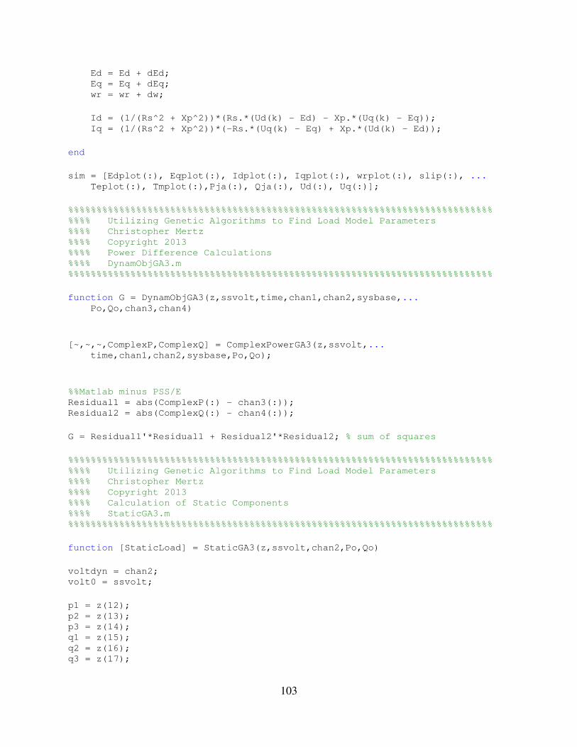
103
Ed = Ed + dEd; Eq = Eq + dEq; wr = wr + dw;
Id = (1/(Rs^2 + Xp^2))*(Rs.*(Ud(k) - Ed) - Xp.*(Uq(k) - Eq)); Iq = (1/(Rs^2 + Xp^2))*(-Rs.*(Uq(k) - Eq) + Xp.*(Ud(k) - Ed));
end
sim = [Edplot(:), Eqplot(:), Idplot(:), Iqplot(:), wrplot(:), slip(:), ... Teplot(:), Tmplot(:),Pja(:), Qja(:), Ud(:), Uq(:)];
%%%%%%%%%%%%%%%%%%%%%%%%%%%%%%%%%%%%%%%%%%%%%%%%%%%%%%%%%%%%%%%%%%%%%%%%%%% %%%% Utilizing Genetic Algorithms to Find Load Model Parameters %%%% Christopher Mertz %%%% Copyright 2013 %%%% Power Difference Calculations %%%% DynamObjGA3.m %%%%%%%%%%%%%%%%%%%%%%%%%%%%%%%%%%%%%%%%%%%%%%%%%%%%%%%%%%%%%%%%%%%%%%%%%%%
function G = DynamObjGA3(z,ssvolt,time,chan1,chan2,sysbase,... Po,Qo,chan3,chan4)
[~,~,~,ComplexP,ComplexQ] = ComplexPowerGA3(z,ssvolt,... time,chan1,chan2,sysbase,Po,Qo);
%%Matlab minus PSS/E Residual1 = abs(ComplexP(:) - chan3(:)); Residual2 = abs(ComplexQ(:) - chan4(:));
G = Residual1'*Residual1 + Residual2'*Residual2; % sum of squares
%%%%%%%%%%%%%%%%%%%%%%%%%%%%%%%%%%%%%%%%%%%%%%%%%%%%%%%%%%%%%%%%%%%%%%%%%%% %%%% Utilizing Genetic Algorithms to Find Load Model Parameters %%%% Christopher Mertz %%%% Copyright 2013 %%%% Calculation of Static Components %%%% StaticGA3.m %%%%%%%%%%%%%%%%%%%%%%%%%%%%%%%%%%%%%%%%%%%%%%%%%%%%%%%%%%%%%%%%%%%%%%%%%%%
function [StaticLoad] = StaticGA3(z,ssvolt,chan2,Po,Qo)
voltdyn = chan2; volt0 = ssvolt;
p1 = z(12); p2 = z(13); p3 = z(14); q1 = z(15); q2 = z(16); q3 = z(17);

104
%% Static ZIP Model for i = 1:length(chan2) Pstatic(i) = Po*(p1*(voltdyn(i)/volt0)^2 + p2*(voltdyn(i)/volt0) + p3); Qstatic(i) = Qo*(q1*(voltdyn(i)/volt0)^2 + q2*(voltdyn(i)/volt0) + q3); end
StaticLoad = [Pstatic(:), Qstatic(:)];
%%%%%%%%%%%%%%%%%%%%%%%%%%%%%%%%%%%%%%%%%%%%%%%%%%%%%%%%%%%%%%%%%%%%%%%%%%% %%%% Utilizing Genetic Algorithms to Find Load Model Parameters %%%% Christopher Mertz %%%% Copyright 2013 %%%% Iteration Based Parks Transformation %%%% ParksTransIter.m %%%%%%%%%%%%%%%%%%%%%%%%%%%%%%%%%%%%%%%%%%%%%%%%%%%%%%%%%%%%%%%%%%%%%%%%%%%
function [Vd, Vq] = ParksTransIter(Vbase,time)
Vm=Vbase; f=60; w=2*pi*f;
%%% per-unit values into sine waves k = 0; for t=1:length(time) k = k+1; Va(k)=Vm(k)*sin(w*time(k)+pi/2); Vb(k)=Vm(k)*sin(w*time(k)-(2*pi/3)+pi/2); Vc(k)=Vm(k)*sin(w*time(k)+(2*pi/3)+pi/2); end;
k = 0; td = time; for t=1:length(time) k = k + 1; Vd(k)=(2/3)*(Va(k)*cos(w*td(k))+Vb(k)*cos(w*td(k)-2*pi/3)+Vc(k)... *cos(w*td(k)+(2*pi/3))); Vq(k)=(2/3)*(Va(k)*-sin(w*td(k))+Vb(k)*-sin(w*td(k)-2*pi/3)+Vc(k)... *-sin(w*td(k)+2*pi/3)); Vo(k)=(1/3)*(Va(k)+Vb(k)+Vc(k)); end
%%%%%%%%%%%%%%%%%%%%%%%%%%%%%%%%%%%%%%%%%%%%%%%%%%%%%%%%%%%%%%%%%%%%%%%%%%% %%%% Utilizing Genetic Algorithms to Find Load Model Parameters %%%% Christopher Mertz %%%% Copyright 2013 %%%% Time Based Parks Transformation %%%% ParksTranstimetest.m %%%%%%%%%%%%%%%%%%%%%%%%%%%%%%%%%%%%%%%%%%%%%%%%%%%%%%%%%%%%%%%%%%%%%%%%%%%
function [Vd, Vq] = ParksTranstimetest(Vbase,timestep,totaltime) Vm=Vbase; f=60; w=2*pi*f;

105
T=totaltime/60; dt=timestep; k=0;
%%% per-unit values into sine waves for t=(0):dt:(totaltime) k=k+1; tt(k)=t; Va(k)=Vm(k)*sin(w*t+pi/2); Vb(k)=Vm(k)*sin(w*t-(2*pi/3)+pi/2); Vc(k)=Vm(k)*sin(w*t+(2*pi/3)+pi/2); end;
k=0; for t=(0):dt:(totaltime) k=k+1; Vd(k)=(2/3)*(Va(k)*cos(w*t)+Vb(k)*cos(w*t-
2*pi/3)+Vc(k)*cos(w*t+(2*pi/3))); Vq(k)=(2/3)*(Va(k)*-sin(w*t)+Vb(k)*-sin(w*t-2*pi/3)+Vc(k)*-
sin(w*t+2*pi/3)); Vo(k)=(1/3)*(Va(k)+Vb(k)+Vc(k)); end