Using Validation Sites and Field Campaigns to Evaluate

Observational and Model Bias (and perhaps correct the bias)

Using Validation Sites and Field Using Validation Sites and Field Campaigns to Evaluate Campaigns to Evaluate

Observational and Model Bias Observational and Model Bias (and perhaps correct the bias)(and perhaps correct the bias)

Tom AckermanBattelle Fellow, PNNL

Professor, University of Washington

2

My primary interest is cloud properties and effects, where the bias errors in our measurements are pretty insignificant compared to model-observation differences

3

A brief history ….A brief history A brief history ……..In the beginning, there were surface measurements

Continuous measurements of state variables Networks => climatology, initialization for forecast models

Then there were field programsShort duration, multiple platforms (aircraft and ground)Process studies => elucidate the physics of the atmosphere

Then there were satellitesGlobal, single platform, one (or a few) instrumentClimatology, spatial snapshots

But, the satellites needed validationMore field programsMultiple locations, repeated efforts

And then there were profiling sitesContinuous measurements of many variables and fluxesProcess studies, satellite evaluation, climatology

4

Ground based (continuous) observations

Satellite observations In Situ (aircraft)

observations

Evaluation

Spatial context Evaluation

Temporal context

Evaluation

Spatial context

5

Types of Ground-based sitesTypes of GroundTypes of Ground--based sitesbased sites

Standard meteorology – radiosondes

Special networks: Baseline Surface Radiation Network (BSRN) or Aerosol Robotic Network (AERONET)

Cloud and Aerosol Profiling (CAP) Sites

6

Japan?

Manus IslandNauruDarwin

7

8

Central Facility

ARM Southern Great Plains ARM Southern Great Plains ARM Southern Great Plains

9

Southern Great Plains Central FacilitySouthern Great Plains Central FacilitySouthern Great Plains Central Facility

10

Bias errors in measurementsBias errors in measurementsBias errors in measurements

Most difficult errors to diagnose By definition, if we know about a bias error, we remove it

How do we find them?Instrument to instrument comparison (water vapor)But, often have only one instrument or we cannot sort out source of inconsistencyInstrument to model comparison (diffuse flux, MPACE)But, which do we trust? (instrument, of course!)Consistency among multiple measurements (single-scatter albedo, aerosol closure experiments)But, can we reduce solution to bias in only one instrument?

11

Some stories from ARMSome stories from ARMSome stories from ARM

12

Story #1: Water vaporStory #1: Water vaporStory #1: Water vapor

ARM has invested more effort and money in the study of water vapor measurements than any other quantityMultiple instrumentationFIVE intensive campaignsMany science team research projectsCountless hours of debate

Revercomb et al., 2003, BAMS (and a host of references)

Soden et al., 2005, JGR and references therein

13

14

15

Microwave Radiometer vs. Vaisala RadiosondeMicrowave Radiometer vs. Microwave Radiometer vs. VaisalaVaisala RadiosondeRadiosonde

16

17

Comparison of Upper Tropospheric Humidity (UTH) from GOES 6.7 m channel with radiosondes and Raman lidar

Comparison of Upper Tropospheric Humidity (UTH) from Comparison of Upper Tropospheric Humidity (UTH) from GOES 6.7 m channel with radiosondes and Raman lidarGOES 6.7 m channel with radiosondes and Raman lidar

18

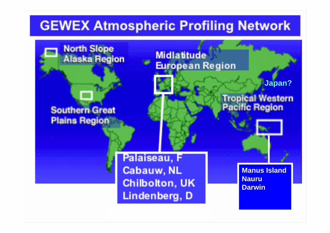
Lessons learnedLessons learnedLessons learned

We can measure water vapor to better than 2% in the column and better than 5% in upper troposphereRadiosondes have to be corrected to get close to this accuracyWe have schemes to do that for Vaisala sondes and they seem to work pretty well (we can quantify this)This information does not seem to be penetrating the operational side of the field (case in point: we cannot get the US Weather Service to switch to Vaisala sondes at Barrow despite our identification of gross errors in the current sondes; Reason: climate record!)

19

Sidebar (courtesy of A. Tomkins)Sidebar (courtesy of A. Sidebar (courtesy of A. TomkinsTomkins))

Fact: we can measure PWV continuously (every 20 seconds) with a MWR to a column error < 2%MWR measurements are accurate over land (and water)Cost of MWR (bulk discount) is ~$100,000Cost of SSM/I is ? (but let’s estimate $20,000,000)So for the cost of 1 SSM/I, I can deploy 200 operational MWRs at land sitesIf you have $20M, which would you prefer?

20

Story #2: Solar diffuse fluxStory #2: Solar diffuse fluxStory #2: Solar diffuse flux

Started with identification of a discrepancy between measured and calculated clear-sky diffuse flux at the SGP Resulted in a large number of model investigationsSpawned one aircraft IOP and two later ground-based IOPsIdentified problem with thermal correction in solar broad-band radiometersCalculated a correction factor that is now standard across all thermal-pile radiometers

21

Observations Thin lines = model with three types of aerosol

22

Michalsky et al.: Diffuse Irradiance IOP in 2003Comparison of 8 BB radiometers

Michalsky et al.: Diffuse Irradiance IOP in 2003Michalsky et al.: Diffuse Irradiance IOP in 2003Comparison of 8 BB radiometersComparison of 8 BB radiometers

23

Lessons learnedLessons learnedLessons learned

Sometimes it ISN’T the modelContinuous, well-calibrated measurements can produce new problems Well-designed experiments can identify the errors and correct themWhy do you care? If you are removing the bias in your model (adding aerosol?) when it is a bias in the instrument ….

24

Story #3: Arctic cloudsStory #3: Arctic cloudsStory #3: Arctic clouds

An Assessment of ECMWF Model Analyses and Forecasts over the North Slope of Alaska Using

Observations from the ARM Mixed-Phase Arctic Cloud Experiment

Shaocheng Xie, Stephen A. Klein, John J. Yio, Anton C. M. Beljaars, Charles N. Long,

and Minghua Zhang

25

Mixed-Phase Arctic Cloud ExperimentMixedMixed--Phase Arctic Cloud ExperimentPhase Arctic Cloud Experiment

Start with MPACE domainCreate domain-average values

Variational analysisTime and space averaging3-hourly values

Compare with ECMWF analysis (6 hourly values)

26

27

28

29

30

31

Ice

Liq.

32

Net Energy loss (surface to atm):

Observations -9.6 W/m2

ECMWF -20.9 W/m2

33

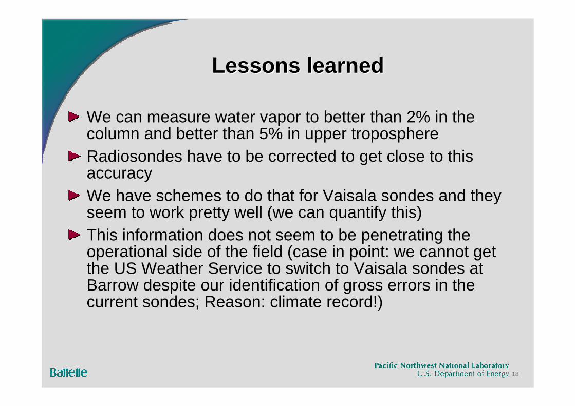
Lessons learnedLessons learnedLessons learned

We can use field data to diagnose model biasesIn this case,

Best results are obtained over the domain => single point values may not be representative of the domainModel does very well in capturing synoptic variation of large scale fieldsModel represents cloud occurrence fairly wellModel clouds have too little liquid water and poor representation of ice/water vertical distributionResults in a severe underestimate of downwelling LW and corresponding errors in surface radiation budget

34

Story #4: Operational comparisonStory #4: Operational comparisonStory #4: Operational comparison

CloudNet projectPI: Prof. Anthony Illingworth, U. ReadingComparison of data from 3 European sites (Cabauw, Chilbolton, Palaiseau) with forecast model output Brilliant webpageBeing extended to Lindenberg and ARM sites

35

Story #5: Heating Rate ProfilesStory #5: Heating Rate ProfilesStory #5: Heating Rate Profiles

Acknowledgements to:Sally McFarlane, Jim Mather, Roger Marchand

36

ARM Tropical Western Pacific SitesARM Tropical Western Pacific SitesARM Tropical Western Pacific Sites

Manus Nauru

37

ARM Data ProcessingARM Data ProcessingARM Data Processing

Heating Rate ProfilesTemperature and water vapor profiles from radiosondes, scaled to microwave radiometer precipitable water and surface temperatureVertical profiles of cloud microphysical properties calculated from ARM millimeter wave radar data (data has 10-second temporal and 45 m vertical resolution)Sample the cloud properties every 5 minutes and perform radiative transfer only on the sampled profiles.Calculate broadband fluxes and vertical profile of heating rates.

38

64 CRM columns x 4 km = 256 km

2.8°

2.8° ~ 300 kmGCM grid column

MMF SchematicMMF SchematicMMF Schematic

39

SimulationsSimulationsSimulations

MMF simulations with CSU model *Run with observed SST valuesStart in January 1998 and run into 2001Second run for 2000 started from different initial conditions

CAM simulationsRun with observed SST values for same period

For the CAM-only runs, we examine output from the gridbox containing the ARM siteFor MMF runs, we examine the average over the 64 CRM columns within the gridbox containing the ARM site

* Model output available to any interested scientists

40

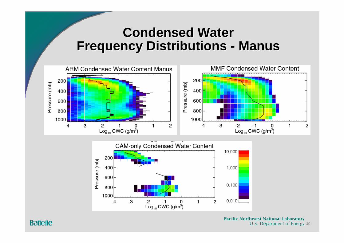
Condensed Water Frequency Distributions - Manus

Condensed Water Condensed Water Frequency Distributions Frequency Distributions -- ManusManus

41

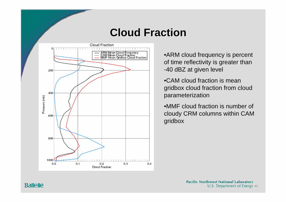
Cloud FractionCloud FractionCloud Fraction

•ARM cloud frequency is percent of time reflectivity is greater than -40 dBZ at given level

•CAM cloud fraction is mean gridbox cloud fraction from cloud parameterization

•MMF cloud fraction is number of cloudy CRM columns within CAM gridbox

42

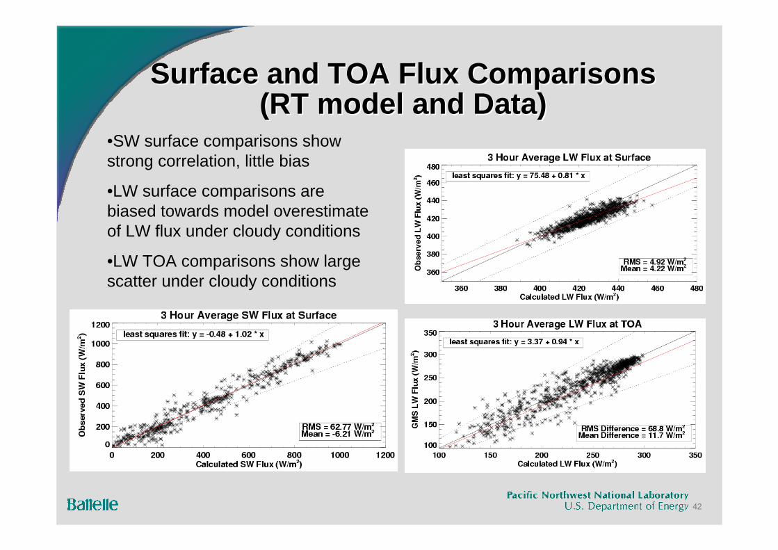
Surface and TOA Flux Comparisons (RT model and Data)

Surface and TOA Flux Comparisons Surface and TOA Flux Comparisons (RT model and Data)(RT model and Data)

•SW surface comparisons show strong correlation, little bias

•LW surface comparisons are biased towards model overestimate of LW flux under cloudy conditions

•LW TOA comparisons show large scatter under cloudy conditions

43

Heating Rates: Clear Sky Heating Rates: Clear Sky Heating Rates: Clear Sky

44

Average Water Vapor ProfilesAverage Water Vapor ProfilesAverage Water Vapor Profiles

45

Heating RatesAll Sky – Clear Sky

Heating RatesHeating RatesAll Sky All Sky –– Clear Sky Clear Sky

46

•CAM has no OLR values below 175 W/m2; larger frequency of very high OLR

•MMF/ARM frequency distributions similar; MMF has more very low OLR values

47

Heating Rates for Various OLR RangesHeating Rates for Various OLR RangesHeating Rates for Various OLR Ranges

48

Lessons learnedLessons learnedLessons learned

We can use routine CAP data to carry out statistical comparisons to identify model biasesResults from this study

MMF reproduces observed water vapor profile and clear sky heating rates better than CAMBoth models have problems with clouds, but CAM are more severeHeating rates errors can be directly tied to deficiencies in cloud propertiesClassification is a very helpful diagnostic

49

SummarySummarySummary

Extensive networks (limited instrumentation)Continuous well-calibrated observations of a few important variablesProvide constraint on model bias

CAP sites (heavily instrumented, few in number)Continuous, well-calibrated observations of many variablesTesting ground for fundamental physics and chemistryDevelopment framework for process modelsEvaluation facility for satellite measurementsEvaluation facility for model performance

50

SummarySummarySummary

Best way (currently) to evaluate model biasContinuous comparison with CAP site data => multiple measurements of variables where possibleIdentify discrepanciesTarget field campaigns at one or more sites to study processes and assign cause to discrepancyCorrectContinue

51

IssuesIssuesIssues

Are we making the “right” measurements?Are there simple data streams that we could generate that would be useful?Do we know the absolute accuracy of the measurements?How good is the data quality assessment?How much measurement detail do we have to communicate to the user (NWP) community in order to make the measurements useful?

52

Thanks for your attention!