Using the SuperLearner R Package L earner Y and X are the data used to t each algorithm (the learning data) newX is not required but can be a helpful shortcut. newX willnotbe used

Using the SuperLearner R Package

Eric Polley

Biometric Research BranchNational Cancer Institute

National Institute of Health

May 2011

1 / 73

Outline

1 SuperLearner

2 Boston Housing

3 ALL data

4 van’t Veer data

2 / 73

SuperLearner

The package is available at:https://github.com/ecpolley/SuperLearner

These slides are available in the package and at:https://github.com/ecpolley/

Need to install R packages nnls and quadprog before installingSuperLearner.

3 / 73

SuperLearner

Table: Main functions in the SuperLearner package

Function Description

SuperLearner fits super learnerCV.SuperLearner cross-validate in super learnerlistWrappers returns list of wrappers in packagewrite.SL.template prediction wrapper templatewrite.screen.template screening wrapper templatewrite.method.template method wrapper template

4 / 73

SuperLearner

fitSL <- SuperLearner(Y = Y,

X = X,

SL.library = c(‘SL.glm’),

family = gaussian(),

method = ‘method.NNLS’,

verbose = TRUE ,

cvControl = list(V = 10))

SuperLearner

5 / 73

SuperLearner

Table: Main arguments for SuperLearner

Name Description Req. Default

Y outcome Y –X data.frame for fit Y –newX data.frame for predict N X

SL.library library of algorithms Y –cvControl list for CV control N –control optional controls N –verbose detailed report N FALSEfamily error distribution N gaussianmethod loss function & model N NNLSid cluster id N –obsWeights observations weights N –

6 / 73

SuperLearner

• Y and X are the data used to fit each algorithm (the learningdata)

• newX is not required but can be a helpful shortcut.newX will not be used to fit the models.

Example with X and newX:1

fit <- glm(Y ~ ., data = X)

out <- predict(fit , newdata = newX)

1The formula Y ∼ . means an additive linear model using all columns of X7 / 73

SuperLearner

newX might be a test set, the interesting values of X forprediction, a stacked data.frame with exposure levels set to beused with for G-computation, etc

newData <- rbind(

cbind(A = 0, subset(X, select = -A)),

cbind(A = 1, subset(X, select = -A))

)

Example setting exposure level for newX

8 / 73

SuperLearner

• family: currently either gaussian() or binomial().• method: either ‘method.NNLS’, ‘method.NNloglik’, or your own

method (see create.method.template()).• verbose: helpful to set this to TRUE to see the progress of the

estimation.

9 / 73

SuperLearner

The ensemble model for “NNLS” is:

ΨSL(W) =

K∑

j=1

αjΨj(W), αj > 0,∑

αj = 1

The ensemble model for “NNloglik” is:

ΨSL(W) =1

1 + exp{−∑Kj=1 αj logitγ

(Ψj(W)

)} , αj > 0,∑

αj = 1

where logitγ is the trimmed logit function to control whenΨj(W) is near 0 or 1.

10 / 73

SuperLearner

There are two types of algorithms that can be used inSL.library:

1 Prediction algorithms. Algorithms that take as input X andY and return a predicted Y value.

2 Screening algorithms. Algorithms designed to reduce thedimension of X. They take as input X and Y and return alogical vector indicating the columns in X passing thescreening. Screening algorithms can be coupled withprediction algorithms to form new prediction algorithms.

11 / 73

listWrappers()

listWrappers ()

Show in R

12 / 73

SuperLearner

There are two ways to specify the algorithms in SL.library:1 A character vector:

c(‘SL.glm’, ‘SL.glmnet’, ‘SL.gam’)

2 A list of character vectors:list(c(‘SL.glm’, ‘screen.corP’), ‘SL.gam’)

If only using prediction algorithms, easier to use the firstmethod.

If using screening algorithms, the list is required. The syntaxfor the elements in the list is the prediction algorithm is first,followed by the screening algorithms. Multiple screeningalgorithms can be used. If a singleton, the default is to apply toall variables.

13 / 73

SuperLearner

see the help documents for SuperLearner for more examples ofSL.library

14 / 73

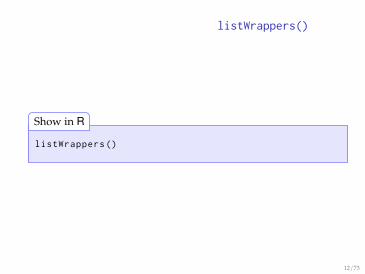
CreatingWrappers

Many algorithms are included in the package (uselistWrappers() for a list of included functions), but these are justenough to get you started.

A few reasons to build your own wrappers:• Want to use an algorithm not currently included• Problem suggests different values for the tuning

parameters• Want to include a range of tuning parameters, not just the

default• Want to select tuning parameters in a different way (e.g.

SL.glmnet selecting λ)• Force variables to be used in step-wise methods

15 / 73

Creating wrappers

The SuperLearner vignette contains a table of tuningparameters for the algorithms in the package

vignette("SuperLearner")

Show in R

16 / 73

Creating wrappers

Example: Creating new prediction algorithm wrapper

17 / 73

Creating wrappers

Consider the polymars algorithm in the polspline package.• continuous outcome Y• data.frame of covariates X• data.frame of covariates newX

fit.mars <- polymars(Y, X)

out <- predict.polymars(fit.mars ,

x = as.matrix(newX))

Now we know how to fit the model and return predictedvalues, next we check out write.SL.template for integrating thecode above into the correct syntax for SuperLearner

18 / 73

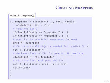
Creating wrappers

SL.template <- function(Y, X, newX , family ,

obsWeights , id, ...) {

# require(’pkg ’)

if(family$family == ’gaussian ’) { }

if(family$family == ’binomial ’) { }

# pred is the predicted responses for newX

pred <- numeric ()

# fit returns all objects needed for predict.SL.*

fit <- list(object = )

# declare class of fit for predict.SL.template

class(fit) <- ’SL.template ’

# return a list with pred and fit

out <- list(pred = pred , fit = fit)

return(out)

}

}

write.SL.template()

19 / 73

Creating wrappers

Table: The arguments passed to a prediction algorithm in SuperLearner

Argument Description

Y the outcome variableX the training data set

(the observations used to fit the model)newX the validation data set

(the observations to return predictions for)family a description of the error distributionid a cluster identificationobsWeights observation weights

You do not need to use all these arguments, but if you use anyof them, the name must match exactly.

20 / 73

Creating wrappers

My.SL.polymars <- function(Y, X, newX ,

family , ...) {

if(family$family =="gaussian") {




}

if(family$family =="binomial") {

# insert estimation function

}

... # next slide

}

SL.polymars

21 / 73

Creating wrappers

What about family = binomial()?

Can leave this blank (or add stop(‘only gaussian’)) if only for aspecific example with continuous outcome.

To be complete, we could look up the code for a binaryoutcome and add this case:

fit.mars <- polyclass(Y, X, cv = 5)

out <- ppolyclass(cov = newX ,

fit = fit.mars)[, 2]

22 / 73

Creating wrappers


family , ...) {





}





}

... # next slide

}

SL.polymars

23 / 73

Creating wrappers

Wrappers need to return 2 values:1 pred: predicted Y values for rows in newX

2 fit: a list with everything needed to use predict method

In the polymars example: For the gaussian case, predict() needs:object = fit.mars

For the binomial case, predict() needs: fit = fit.mars

Note: SuperLearner does not use the fit list. If you do not planto use the function predict.SuperLearner you can leave the fitobject as: fit <- vector("list", length = 0)

24 / 73

Creating wrappers


family , ...) {





fit <- list(object = fit.mars)

}





fit <- list(fit = fit.mars)

}

... # next slide

}

SL.polymars

25 / 73

Creating wrappers

Final step is putting everything together into a list object. Thelist must have 2 elements and the names must be pred and fit

Can also assign a class to the fit list. This will be used to lookup the correct predict method. I’m using S3 methods here. Thisis only important if using predict.SuperLearner afterwards.

See Chambers (2008) Software for Data Analysis for details on S3and S4 methods.

26 / 73

Creating wrappers


family , ...) {

... # previous slides

out <- list(pred = pred , fit = fit)

class(out$fit) <- c("SL.polymars")

return(out)

}

SL.polymars

Note: out is just a temporary variable name here.

The function should match SL.polymars in the SuperLearnerpackage.

27 / 73

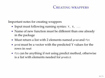
Creating wrappers

Important notes for creating wrappers• Input must following naming syntax: Y, X, ...

• Name of new function must be different than one alreadyin the package

• Must return a list with 2 elements named pred and fit

• pred must be a vector with the predicted Y values for therows in newX

• fit can be anything if not using predict method, otherwiseis a list with elements needed for predict

28 / 73

Creating wrappers

predict.SL.template <- function (object ,

newdata , family , X = NULL , Y = NULL , ...)

{

pred <- numeric ()

return(pred)

}

predict.SL.template

29 / 73

Creating wrappers

predict.SL.polymars <-

function (object , newdata , family , ...) {

if (family$family == "gaussian") {

pred <- predict.polymars(object = object$object ,

x = as.matrix(newdata ))

}

if (family$family == "binomial") {

pred <- ppolyclass(cov = newdata ,

fit = object$fit)[, 2]

}

return(pred)

}

predict.SL.polymars

30 / 73

Creating wrappers

Example: creating screening algorithm

31 / 73

Creating wrappers

screen.template <- function (Y, X, family ,

obsWeights , id , ...) {

# require(’pkg ’)


}


}

# whichVariable is a logical vector ,

# TRUE indicates variable will be used

whichVariable <- rep(TRUE , ncol(X))

return(whichVariable)

}

screening template

32 / 73

Creating wrappers

Table: The arguments passed to a screening algorithm in SuperLearner

Argument Description

Y the outcome variableX the training data set

(the observations used to fit the model)family a description of the error distributionid a cluster identificationobsWeights observation weights

You do not need to use all these arguments, but if you use anyof them, the name must match exactly.

33 / 73

screen.randomForest <- function (Y, X,

family , nVar = 10, ntree = 1000, ...) {


rank.rf.fit <- randomForest(Y ~ .,

data = X, ntree = ntree)

}


rank.rf.fit <- randomForest(

y = as.factor(Y), x = X,

ntree = ntree)

}

whichVariable <- as.logical(

rank(-rank.rf.fit$importance) <= nVar)

return(whichVariable)

}

screen.randomForest

34 / 73

Boston Housing example

The outcome variable is the median home value (cmedv) for the506 census tracts of Boston from the 1970 census.

The covariates are a mix of geographical and socioeconomicvariables, like per capita crime rate (crim), average number ofrooms per house (rm), distance to Boston employment centres(dis), indictor of tract being on the Charles river (chas), etc.

35 / 73

Boston Housing

The Boston Housing data can be found in the mlbenchpackage.

library(mlbench)

data(BostonHousing2)

# convert factors to numeric

BostonHousing2$chas

<- as.numeric(BostonHousing2$chas=="1")

# select subset of variables

DATA <- BostonHousing2[, c("cmedv", "crim", "zn",

"indus", "chas", "nox", "rm", "age", "dis",

"rad", "tax", "ptratio", "b", "lstat")]

Load the data

36 / 73


First need to decide which prediction algorithms to include inthe library

37 / 73

Boston Housing

Algorithm Description Package

glm linear model statsrandomForest random Forest randomForestbagging bootstrap aggregation of trees ipredgam generalized additive models gamgbm gradient boosting gbmnnet neural network nnetpolymars polynomial spline regr. polsplinebart Bayesian additive regr. trees BayesTreeglmnet elastic net glmnetsvm support vector machine e1071bayesglm Bayesian glm armstep stepwise glm stats

38 / 73

Boston Housing

One algorithm to consider is the generalized additive modelalgorithm. This algorithm has a tuning parameter for thedegrees of freedom in the smoother. I have set this to be 2 inSL.gam but we might want to consider larger values.

We could create an entirely new wrapper for gam and df = 3, orwe can write a wrapper for the wrapper and only change thedegrees of freedom value.

39 / 73

Boston Housing

look at SL.gam to see how the degrees of freedom parameter isspecified:

40 / 73

SL.gam <- function(Y, X, newX ,

family , obsWeights , deg.gam = 2, ...)

{

... # model: Y ~ s(X, deg.gam)

# see full functions for details

fit.gam <- gam::gam(gam.model , data = X,

family = family ,

control = gam.control(maxit = 50, bf.maxit = 50),

weights = obsWeights)

pred <- predict(fit.gam , newdata = newX ,

type = "response")

... # returns list here

}

SL.gam

41 / 73

Boston Housing

The SL.gam function contains the argument deg.gam = 2.

Wrappers can have additional arguments, but they must havedefault values.

42 / 73


For the new wrapper, only need to change the value of deg.gam.Use . . . to pass everything else between SL.gam.3 and SL.gam.

SL.gam.3 <- function (..., deg.gam = 3) {

SL.gam(..., deg.gam = deg.gam)

}

Adjusting deg.gam in SL.gam

Easy to create new wrappers by changing tuning parametervalues. Check the code for the wrappers by typing the name ofthe function without parentheses to see what tuning parametervalues are in the arguments.

43 / 73

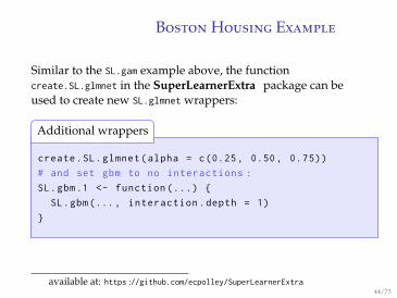
Boston Housing Example

Similar to the SL.gam example above, the functioncreate.SL.glmnet in the SuperLearnerExtra2 package can beused to create new SL.glmnet wrappers:

create.SL.glmnet(alpha = c(0.25, 0.50, 0.75))

# and set gbm to no interactions:

SL.gbm.1 <- function (...) {

SL.gbm(..., interaction.depth = 1)

}

Additional wrappers

2available at: https://github.com/ecpolley/SuperLearnerExtra44 / 73


SL.library <- c("SL.gam",

"SL.gam.3", "SL.gam.4",

"SL.gam.5", "SL.gbm.1",

"SL.gbm", "SL.glm",

"SL.glmnet", "SL.glmnet .0.25",

"SL.glmnet.alpha .0.5", "SL.glmnet .0.75",

"SL.polymars", "SL.randomForest",

"SL.ridge", "SL.svm",

"SL.bayesglm", "SL.step",

"SL.step.interaction",

"SL.bart")

SL.library

45 / 73


fitSL <- SuperLearner(Y = log(DATA$cmedv),

X = subset(DATA , select = -c(cmedv)),

SL.library = SL.library ,

family = gaussian ()

)

fitSL

46 / 73

Risk Coef

SL.gam_All 0.03834031 0.0000000

SL.gam.3_All 0.03666449 0.0000000

SL.gam.4_All 0.03589859 0.0000000

SL.gam.5_All 0.03529692 0.0000000

SL.gbm.1_All 0.03040543 0.0000000

SL.gbm.2_All 0.02501729 0.0000000

SL.glm_All 0.03754472 0.0000000

SL.glmnet_All 0.03765112 0.0000000

SL.glmnet.alpha25_All 0.03754278 0.0000000



SL.polymars_All 0.04587432 0.0000000

SL.randomForest_All 0.02105987 0.2956277

SL.ridge_All 0.03753661 0.0000000

SL.svm_All 0.02678290 0.0000000

SL.bayesglm_All 0.03754318 0.0000000

SL.step_All 0.03753337 0.0000000

SL.step.interaction_All 0.02411940 0.3099166

SL.bart_All 0.02003557 0.3944557

47 / 73

Boston Housing

Table: Elements of the output from SuperLearner

Name Description

SL.predict super learner predicted values for newX

coef coefficient for each algorithmlibraryNames names of algorithms in librarylibrary.predict matrix of predicted values for newX from

each algorithm in the librarycvRisk V-fold cross-validated risk for each algorithm

in the library

48 / 73

Boston Housing

The final super learner prediction model is the weightedcombination of the library algorithms where the estimates ofthe weights can be found with coef(fitSL).

To attain predictions on new observations (not in newX), thepredict function will usually work. If you created newwrappers, you also need to create predict S3 methods for thosenew wrappers.

49 / 73

Boston Housing

SuperLearner is a model selection algorithm. It does not containa good estimate for model assessment (you could use there-substitution method to estimate the risk but this isoptimistic).

Our suggestion to assess the performance of the super learneris to run CV.SuperLearner (example in the next case study).

50 / 73

ALL example

• The outcome variable is an indicator of the molecularbiology of the cancer tissue, either Negative or BCR/ABL.

• The sample consists of 79 individuals(42 Neg, 37 BCR/ABL).

• The data contain 2200 features (X) to be used after thefiltering steps.

• Need to select algorithms appropriate for a binaryoutcome and a large number of covariates.

51 / 73

ALL

# source ("http://bioconductor.org/biocLite.R")

# biocLite ()

# biocLite ("ALL")

library(ALL)

library(genefilter)

data(ALL)

load ALL data

The next 2 slides are the processing steps following inGentleman, Huber and Carey (2008) “Supervised MachineLearning” in Bioconductor Case Studies.

52 / 73

# restrict to only the NEG and BCR/ABL outcomes

bcell <- grep("^B", as.character(ALL$BT))

moltyp <- which(as.character(ALL$mol.biol)

%in% c("NEG", "BCR/ABL"))

ALL_bcrneg <- ALL[, intersect(bcell , moltyp )]

#drops unused levels

ALL_bcrneg$mol.biol <- factor(ALL_bcrneg$mol.biol)

# filter features

ALLfilt_bcrneg <- nsFilter(ALL_bcrneg ,

var.cutoff = 0.75)$eset

53 / 73

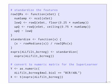
# standardize the features

rowIQRs <- function(eSet) {

numSamp <- ncol(eSet)

lowQ <- rowQ(eSet , floor (0.25 * numSamp ))

upQ <- rowQ(eSet , ceiling (0.75 * numSamp ))

upQ - lowQ

}

standardize <- function(x) {

(x - rowMedians(x)) / rowIQRs(x)

}

exprs(ALLfilt_bcrneg) <- standardize(

exprs(ALLfilt_bcrneg ))

# convert to numeric matrix for the SuperLearner

Y <- as.numeric(

ALLfilt_bcrneg$mol.biol == "BCR/ABL")

X <- t(exprs(ALLfilt_bcrneg ))

54 / 73

ALL

Possible prediction algorithms include:• k-nearest neighbors• elastic net (penalized regression)• random forest

These algorithms have tuning parameters:• knn: k• glmnet: α• randomForest: mtry and nodesize

55 / 73

ALL

tuneGrid <- expand.grid(mtry = c(500, 1000, 2200),

nodesize = c(1, 5, 10))

for(mm in seq(nrow(tuneGrid ))) {

eval(parse(file = "", text =

paste("SL.randomForest.", mm,

"<- function (..., mtry = ", tuneGrid[mm, 1],

", nodesize = ", tuneGrid[mm, 2], ") {

SL.randomForest (..., mtry = mtry ,

nodesize = nodesize) }", sep = "")))

}

randomForest

56 / 73

ALLThe code above is hard to follow, but I’m doing the same thingwe did with SL.gam.3 just in a for loop.

> SL.randomForest .1

function (..., mtry = 500, nodesize = 1) {


nodesize = nodesize) }




nodesize = nodesize) }




nodesize = nodesize) } 57 / 73

ALL

Add additional knn wrappers using functions inSuperLearnerExtra3

create.SL.knn(k = c(k = 20, 30, 40, 50))

create.SL.knn

3available at: https://github.com/ecpolley/SuperLearnerExtra58 / 73

ALL

SL.library <- c("SL.knn",

"SL.knn.20",

"SL.knn.30",

"SL.knn.40",

"SL.knn.50",

"SL.randomForest",

"SL.glmnet",

"SL.glmnet .0.25",

"SL.glmnet .0.5",

"SL.glmnet .0.75",

"SL.mean",

paste("SL.randomForest.",

seq(nrow(tuneGrid)), sep = ""))

SL.library

59 / 73

ALL

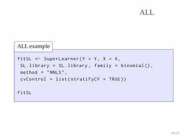
fitSL <- SuperLearner(Y = Y, X = X,

SL.library = SL.library , family = binomial(),

method = "NNLS",

cvControl = list(stratifyCV = TRUE))

fitSL

ALL example

60 / 73

Risk Coef

SL.knn_All 0.20658228 0.00000000

SL.knn20_All 0.22423347 0.00000000

SL.knn30_All 0.22299664 0.00000000

SL.knn40_All 0.23445986 0.00000000

SL.knn50_All 0.23920321 0.00000000

SL.randomForest_All 0.12418009 0.00000000

SL.glmnet_All 0.08430633 0.98039534




SL.randomForest .1_All 0.13103528 0.00000000









61 / 73

ALL

fitSL.CV <- CV.SuperLearner(Y = Y, X = X,


V = 20, family = binomial(),

method = "method.NNLS",


summary(fitSL.CV)

# can also print the LaTeX table

# requires Hmisc package

# latex(summary(fitSL.CV))

CV.SuperLearner

62 / 73

Algorithm subset Risk SE Min Max

SuperLearner – 0.101 0.020 0.003 0.382Discrete SL – 0.095 0.021 0.004 0.347SL.knn(10) All 0.212 0.018 0.070 0.460SL.knn(20) All 0.220 0.011 0.152 0.322SL.knn(30) All 0.223 0.008 0.192 0.274SL.knn(40) All 0.232 0.006 0.187 0.268SL.knn(50) All 0.238 0.004 0.218 0.260SL.randomForest All 0.120 0.014 0.026 0.256SL.glmnet(α = 1.0) All 0.088 0.022 0.002 0.395SL.glmnet(α = 0.25) All 0.113 0.022 0.007 0.451SL.glmnet(α = 0.50) All 0.106 0.023 0.004 0.447SL.glmnet(α = 0.75) All 0.093 0.021 0.004 0.347SL.mean All 0.249 0.004 0.242 0.251SL.randomForest.1 All 0.125 0.014 0.034 0.269SL.randomForest.2 All 0.114 0.014 0.023 0.250SL.randomForest.3 All 0.111 0.015 0.016 0.238SL.randomForest.4 All 0.123 0.014 0.036 0.264SL.randomForest.5 All 0.117 0.014 0.023 0.262SL.randomForest.6 All 0.110 0.015 0.015 0.252SL.randomForest.7 All 0.126 0.014 0.034 0.266SL.randomForest.8 All 0.117 0.014 0.023 0.259SL.randomForest.9 All 0.110 0.015 0.013 0.245

63 / 73

van’t Veer example

• 97 breast cancer patients followed for 5 years.• Outcome is binary yes/no recur in 5 years (we do not have

the date of recurrence)• 7 clinical variables are available (age, tumor grade, etc.)• 4348 gene expression values post-filtering

64 / 73

van’t Veer data

The original data is available at:http://www.rii.com/publications/2002/vantveer.html

65 / 73

van’t Veer

One interesting “screening” is to consider the predictionalgorithms on only the clinical variables or on only the geneexpression variables.

screen.clinical <- function (...){

return(c(rep(TRUE , 7), rep(FALSE , 4348)))

}

screen.array <- function (...){

return(c(rep(FALSE , 7), rep(TRUE , 4348)))

}

screening

66 / 73

SL.library <- list(

c("SL.knn", "All", "screen.clinical",

"screen.corP", "screen.corP .01", "screen.glmnet"),

c("SL.knn.20", "All", "screen.clinical",

"screen.corP", "screen.corP .01", "screen.glmnet"),

c("SL.glmnet", "screen.corRank .50",

"screen.corRank .20"),

c("SL.glmnet .0.75", "screen.corRank .50",






c("SL.randomForest", "screen.clinical",

"screen.corP .01", "screen.glmnet"),

c("SL.bagging", "screen.clinical",


c("SL.bart", "screen.clinical",


c("SL.mean", "All"))

67 / 73

van’t Veer

fitSL <- SuperLearner(Y = surv.resp , X = X,


family = binomial(),


control = list(saveFitLibrary = FALSE))

fitSL

SuperLearner

68 / 73

van’t Veer

Risk Coef

...

SL.knn_screen.corP .01 0.2129897 0.27517459

...

SL.glmnet_screen.corRank .20 0.2210815 0.22256164

...

SL.randomForest_clinical 0.2151708 0.08636558

...

SL.bart_clinical 0.2084039 0.41589818

fitSL

Only presenting results for non-zero coefficients. Table doesnot fit on a slide.

69 / 73

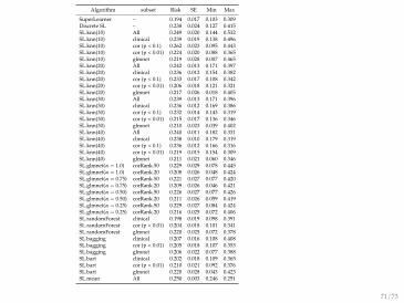
van’t Veer

fitSL.CV <- CV.SuperLearner(Y=surv.resp , X=X,

V = 20,


family = binomial(),



summary(fitSL.CV)

CV.SuperLearner

70 / 73

Algorithm subset Risk SE Min Max

SuperLearner – 0.194 0.017 0.103 0.309Discrete SL – 0.238 0.024 0.127 0.415SL.knn(10) All 0.249 0.020 0.144 0.532SL.knn(10) clinical 0.239 0.019 0.138 0.496SL.knn(10) cor (p < 0.1) 0.262 0.023 0.095 0.443SL.knn(10) cor (p < 0.01) 0.224 0.020 0.088 0.365SL.knn(10) glmnet 0.219 0.028 0.007 0.465SL.knn(20) All 0.242 0.013 0.171 0.397SL.knn(20) clinical 0.236 0.012 0.154 0.382SL.knn(20) cor (p < 0.1) 0.233 0.017 0.108 0.342SL.knn(20) cor (p < 0.01) 0.206 0.018 0.121 0.321SL.knn(20) glmnet 0.217 0.026 0.018 0.405SL.knn(30) All 0.239 0.013 0.171 0.396SL.knn(30) clinical 0.236 0.012 0.169 0.386SL.knn(30) cor (p < 0.1) 0.232 0.014 0.143 0.319SL.knn(30) cor (p < 0.01) 0.215 0.017 0.136 0.346SL.knn(30) glmnet 0.210 0.023 0.039 0.402SL.knn(40) All 0.240 0.011 0.182 0.331SL.knn(40) clinical 0.238 0.010 0.179 0.319SL.knn(40) cor (p < 0.1) 0.236 0.012 0.166 0.316SL.knn(40) cor (p < 0.01) 0.219 0.015 0.154 0.309SL.knn(40) glmnet 0.211 0.021 0.060 0.346SL.glmnet(α = 1.0) corRank.50 0.229 0.029 0.078 0.445SL.glmnet(α = 1.0) corRank.20 0.208 0.026 0.048 0.424SL.glmnet(α = 0.75) corRank.50 0.221 0.027 0.077 0.420SL.glmnet(α = 0.75) corRank.20 0.209 0.026 0.046 0.421SL.glmnet(α = 0.50) corRank.50 0.226 0.027 0.077 0.426SL.glmnet(α = 0.50) corRank.20 0.211 0.026 0.059 0.419SL.glmnet(α = 0.25) corRank.50 0.229 0.027 0.084 0.424SL.glmnet(α = 0.25) corRank.20 0.216 0.025 0.072 0.406SL.randomForest clinical 0.198 0.019 0.098 0.391SL.randomForest cor (p < 0.01) 0.204 0.018 0.101 0.341SL.randomForest glmnet 0.220 0.025 0.072 0.378SL.bagging clinical 0.207 0.016 0.108 0.408SL.bagging cor (p < 0.01) 0.205 0.018 0.107 0.353SL.bagging glmnet 0.206 0.022 0.077 0.388SL.bart clinical 0.202 0.018 0.109 0.365SL.bart cor (p < 0.01) 0.210 0.021 0.092 0.376SL.bart glmnet 0.220 0.028 0.043 0.423SL.mean All 0.250 0.003 0.246 0.251

71 / 73

R packages

install.packages(c("glmnet","randomForest",

"class", "gam", "gbm", "nnet", "polspline",

"MASS", "e1071", "stepPlr", "arm", "party",

"spls", "LogicReg", "nnls", "multicore",

"SIS", "BayesTree", "quadprog", "ipred",

"mlbench", "rpart", "caret", "mda", "earth"),

type="source",

repos="http://cran.cnr.Berkeley.edu",

dependencies=c("Depends", "Imports"))

# missing DSA , not available on CRAN

Installing suggested packages

Can remove type = ‘source’ if system not setup to installpackages from source.

72 / 73

Colophon

• Slides created with LATEX package Beamer• Code blocks adapted from the tikzDevice R package• LATEX package tikz and sweave for code styles• R version 2.13.0 and SuperLearner version 2.0-1• Other packages: arm 1.4-10, BayesTree 0.3-1, caret 4.88,

class 7.3-3, DSA 3.1.4, e1071 1.5-25, earth 2.6-2, gam 1.04,gbm 1.6-3, glmnet 1.6, Hmisc 3.8-3, ipred 0.8-11, leaps 2.9,lme4 0.999375-39, LogicReg 1.4.10, MASS 7.3-13, mda 0.4-2,mlbench 2.1-0, modelUtils 3.1.4, nnet 7.3-1, nnls 1.3,party 0.9-9994, polspline 1.1.5, quadprog 1.5-4,randomForest 4.6-2, rpart 3.1-50, SIS 0.6,

73 / 73

Documents

Using the SuperLearner R Package L earner Y and X are the data used to t each algorithm (the learning data) newX is not required but can be a helpful shortcut. newX willnotbe used