Using Temporal Logics to Express Search Control …fbacchus/Papers/tlplanaij.pdfUsing Temporal Logics to Express Search Control Knowledge for Planning Fahiem Bacchus Dept. Of Computer

Using Temporal Logics to Express Search ControlKnowledge for Planning�

Fahiem BacchusDept. Of Computer Science

University of TorontoToronto, Ontario

Canada, M5S [email protected]

Froduald KabanzaDept. De Math et Informatique

Universite De SherbrookeSherbrooke, Quebec

Canada, J1K [email protected]

January 21, 2000

Abstract

Over the years increasingly sophisticated planning algorithms have been developed. Thesehave made for more efficient planners, but unfortunately these planners still suffer from com-binatorial complexity even in simple domains. Theoretical results demonstrate that planning isin the worst case intractable. Nevertheless, planning in particular domains can often be madetractable by utilizing additional domain structure. In fact, it has long been acknowledged thatdomain independent planners need domain dependent information to help them plan effec-tively. In this work we present an approach for representing and utilizing domain specific con-trol knowledge. In particular, we show how domain dependent search control knowledge canbe represented in a temporal logic, and then utilized to effectively control a forward-chainingplanner. There are a number of advantages to our approach, including a declarative semanticsfor the search control knowledge; a high degree of modularity (new search control knowl-edge can be added without affecting previous control knowledge); and an independence of thisknowledge from the details of the planning algorithm. We have implemented our ideas in theTLPLAN system, and have been able to demonstrate its remarkable effectiveness in a widerange of planning domains.

1 Introduction

The classical planning problem, i.e., finding a finite sequence of actions that will transform a giveninitial state to a state that satisfies a given goal, is computationally difficult. In the traditional

�This research was supported by the Canadian Government through their IRIS project and NSERC programs. Apreliminary version of the results of this paper were presented at the European Workshop on AI Planning 1995 andappears in [3]. This was done when Fahiem Bacchus was at the

1

context, in which actions are represented using the STRIPS representation and the initial and goalstates are specified as lists of literals, even restricted versions of the planning problem are knownto be PSPACE-complete [20].

Although informative, these worst case hardness results do not mean that computing plans isimpossible. As we will demonstrate many domains offer additional structure that can ease thedifficult of planning.

There are a variety of mechanisms that can be used to exploit structure so as to make planningeasier. Abstraction and the related use of hierarchical task network (HTN) planners have been stud-ied in the literature and utilized in planning systems [36, 48, 62, 55], also mechanisms for searchcontrol have received much attention. Truly effective planners will probably utilize a number ofmechanisms. Hence, it is important that each of these mechanisms be developed and understood.This paper makes a contribution to the development of mechanisms for search control.

Search control is useful since most planning algorithms employ search to find plans. Planningresearchers have identified a variety of spaces in which this search can be performed. However,these spaces are all exponential in size, and blind search in any of them is ineffective. Hence, a keyproblem facing planning systems is that of guiding or controlling search.

The idea of search control is not new—the notion of search heuristics is one of the fundamentalideas in AI. Most planning implementations use heuristically guided search, and various sophis-ticated heuristics have been developed for guiding planning search [24, 30]. Knowledge-basedsystems for search control have also been developed. In particular, knowledge bases of forwardchaining rules have been used to guide search (these are in essence expert-systems for guidingsearch). The SOAR system was the first to utilize this approach [38], and a refined version is aprominent part of the PRODIGY system [59]. A similar rule-based approach to search control hasalso been incorporated into the UCPOP implementation [7], and a more procedural search controllanguage has also been developed [43]. A key difference between the knowledge-based searchcontrol systems and various search heuristics is that knowledge-based systems generally rely ondomain dependent knowledge, while the search heuristics are generally domain independent.

The work reported on here is a new approach to knowledge-based search control. In particu-lar, we utilize domain dependent search control knowledge, but we utilize a different knowledgerepresentation and a different reasoning mechanism than previous approaches.

In previous work, search control has utilized the current state of the planning algorithm toprovide advice as to what to do next. This advice has been computed either by evaluating domainindependent heuristics on the current state of the planner, or by using the current state to trigger aset of forward chaining rules that ultimately generate the advice.

Our approach differs. First, the control it provides can in general depend on the entire sequenceof predecessors of the current state not only on the current state. As we will demonstrate this facil-itates more effective search control. And second, the search control information we use does notmake reference to the state of the planning algorithm, rather it only makes reference to propertiesof the planning domain. It is up to the planning algorithm to take advantage of this information,by mapping that information into properties of its own internal state. This means that althoughthe control information we utilize is domain dependent, the provider of this information need not

2

know anything about the planning algorithm.Obtaining domain dependent search control information does of course impose a significant

overhead when modeling a planning domain.1 This overhead can only be justified by increasedplanning efficiency. In this paper we will give empirical evidence that such information can makea tremendous difference in planning efficiency. In fact, as we will show, it can often convert anintractable planning problem to a tractable one; i.e., it can often be the only way in which automaticplanning is possible.

Our work makes an advance over previous mechanisms for search control in two crucial areas.First, it provides far greater improvements to planning efficiency that previous approaches. Wecan sometimes obtain polynomial time planners with relatively simply control knowledge. In ourempirical tests, none of the other approaches have yielded speedups of this magnitude. And second,although our approach is of course more difficult to use than domain-independent search heuristics,it seems to be much easier to use than the previous rule-based mechanisms.2 In sum, our approachoffers a lower overhead mechanism that yields superior end results.

Our approach uses a first-order temporal logic to represent search control knowledge. By uti-lizing a logic we gain the advantage of providing a formal semantics for the search control knowl-edge, and open the door to more sophisticated off-line reasoning for generating and manipulatingthis knowledge. In other words, we have a declarative representation of the search control knowl-edge which facilitates a variety of uses. Through examples we will demonstrate that this logicallows us the express effective search control information, and furthermore that this information isquite natural and intuitive.3

Logics have been previously used in work on planning. In fact, perhaps the earliest work onplanning was Green’s approach that used the situation calculus [25]. Subsequent work on planningusing logic has included Rosenschein’s use of dynamic logic [46], and Biundo et al.’s use of tem-poral logic [10, 12, 11, 53]. However, all of this work has viewed planning as a theorem provingproblem. In this approach the initial state, the action effects, and the goal, are all encoded as log-ical formulas. Then, following Green, plans are generated by attempting to prove (constructively)that a plan exists. Planning as theorem proving has to date suffered from severe computationalproblems, and this approach has not yet yielded an effective planner.

Our approach uses logic in a completely different manner. In particular, we are not viewingplanning as theorem proving. Instead we utilize traditional planning representations for actions andstates, and we generate plans by search. Theorem provers also employ search to generate plans.However, their performance seems to be hampered by the fact that they must search in the spaceof proofs, a space that has no clear relation to the structure of plans.4

1We shall argue in Section 9 that this overhead is manageable.2The more recently developed procedural search control mechanisms seem to be just as hard to use [43].3In fact, it can be argued that this information is no different from our knowledge of actions; it is simply part of

our store of domain knowledge. Hence, there is no reason why it should not be utilized in our planning systems.4The most promising approaches to planning as theorem proving have utilized insights from non-theorem proving

approaches to provide specialized guidance to the theorem proving search. For example, Biundo and Stephan [53]have utilized ideas from refinement planning to guide the theorem proving process.

3

In our approach we use logic solely to express search control knowledge. We then show howthis knowledge can be used to control search in a simple forward-chaining planner. We explainwhy such a planner is particularly effective at utilizing information expressed in the chosen tem-poral logic. We have implemented this combination of a simple forward-chaining planner andtemporal logic search control in a system we call the TLPLAN system. The resulting system is asurprisingly effective and powerful planner. The planner is also very flexible, for example, it canplan with conditional actions expressed using the full ADL language [44], and can handle certaintypes of resource constraints. We will demonstrate its effectiveness empirically on a number oftest domains.

Forward chaining planners have fallen out of favor in the AI planning community. This is dueto the fact that there are alternate spaces in which searching for plans is generally more effec-tive. Partial order planners that search in the space of partially ordered plans have been shown topossess a number of advantages [9, 41]. And more recently planners that search over GRAPH-PLAN graphs [13] or over models of propositional theories representing the space of plans [32],have been shown to be quite effective. Nevertheless, as we will demonstrate, the combinationof domain-specific search control information, expressed in the formalism we suggest, and a for-ward chaining planner significantly outperforms competing planners in a range of test domains.It appears that forward chaining planners, despite their disadvantages, are significantly easier tocontrol, and hence the ultimate choice of planning technology may still be open to question. Thepoint that forward chaining planners are easier to control has also been argued by McDermott [40]and Bonet et al. [14]. They have both presented planning systems based on heuristically controlledforward chaining search. They have methods for automatically generating heuristics, but there isstill considerable work to be done before truly effective control information can be automaticallyextracted for a particular planning problem. As a result the performance of their systems is not yetcompetitive with the fastest domain-independent planning systems like BLACKBOX [33] or IPP[37] (check, e.g., the performance of the HSP planning system [14] at the recent AIPS’98 planningcompetition [1]). In this paper we utilize domain-specific search control knowledge, and presentresults that demonstrate that with this kind of knowledge our approach can reach a new level ofperformance in AI planning.

In the rest of the paper we will describe the temporal logic we use to express domain dependentsearch control knowledge. Then we present an example showing how control information can beexpressed in this logic. In Section 4 we show how a planning algorithm can be designed thatutilizes this information, and in section 6 we describe the TLPLAN system, a planner we haveconstructed based on these ideas. To show the effectiveness of our approach we present the resultsof a number of empirical studies in section 7. There has been other work on domain specific controlfor planning systems, and HTN planners also employ extensive domain specific information. Wecompare our approach with these works in Section 9. Finally, we close with some conclusions anda discussion of what we feel are some of the important research issues suggested by our work.

4

2 First-order Linear Temporal Logic

We use as our language for expressing search control knowledge a first-order version of lineartemporal logic (LTL) [19]. The language starts with a standard first-order language, �, containingsome collection of constant, function, and predicate symbols, along with a collection of variables.We also include in the language the propositional constants TRUE and FALSE, which are treatedas atomic formulas. LTL adds to � the following temporal modalities: U (until), � (always), �(eventually), and � (next). The standard formula formation rules for first-order logic are aug-mented by the following rules: if �� and �� are formulas then so are �� U ��, ��, ��, and ��.Note that the first-order and temporal formula formation rules can be applied in any order, so, e.g.,quantifiers can scope temporal modalities allowing quantifying into modal contexts. We will callthe extension of � to include these temporal modalities �� .

�� is interpreted over sequences of worlds, and the temporal modalities are used to assertproperties of these sequences. In particular, the temporal modalities have the following intuitiveinterpretations: �� means that � holds in the next world; �� means that � holds in the currentworld and in all future worlds; �� means that � either holds now or in some future world; and�� U�� means that either now or in some future world �� holds and until that world �� holds. Theseintuitive semantics are, however, only approximations of the true semantics of these modalities. Inparticular, the formulas � , ��, and �� can themselves contain temporal modalities so when we say,e.g., that � holds in the next world we really mean that � is true of the sequence of worlds thatstarts at the next world. The precise semantics are given below.

The formulas of �� are interpreted over models of the form M � �� where M is asequence of worlds. We will sometimes refer to this sequence of worlds as the timeline. Everyworld �� is a model for the base first-order language �. Furthermore, we require that each �� sharethe same domain of discourse D. A constant domain of discourse across all worlds allows us toavoid the difficulties that can arise when quantifying into modal contexts [23].

We specify the semantics of the formulas of our language with the following set of interpre-tation rules. Let �� be the �’th world in the timeline M, � be a variable assignment function thatmaps the variables of �� to the domain D, and �� and �� be formulas of �� .

� If �� is an atomic formula then �M� �� iff �� . That is, atomic formulasare interpreted in the world �� under the variable assignment � according to the standardinterpretation rules for first-order logic.

� The logical connectives are handled in the standard manner.

� �M� �� iff �M� �� for all � , where � �� is a variableassignment function identical to � except that it maps � to .

� �M� �� U�� iff there exists � � such that �M� �� and for all �, � � �we have �M� �� : �� is true until �� is achieved.

� �M� �� iff �M� �� : �� is true in the next state.

5

� �M� �� iff there exists � � such that �M� �� : �� is eventually true.

� �M� �� iff for all � � we have �M� �� : �� is true in all states from thecurrent state on.

Finally, we say that the model M satisfies a formula � (M �� ) iff �M� �� (i.e., theformula must be true in the initial world). It is not difficult to show that if � has no free variablesthen the specific variable assignment function � is irrelevant.

2.1 Discussion

One of the keys to understanding the semantics of temporal formulas is to realize that the temporalmodalities move us along the timeline. That is, the formulas that are inside of a temporal modalityare generally interpreted not at the current world, ��, but at some world further along the sequence,�� with � �. This can be seen from the semantic rules given above. The expressiveness of�� arises from its ability to nest temporal modalities and thus express complex properties of thetimeline.

Another point worth making is that both the eventually and always modalities are in fact equiv-alent to until assertions. In particular, �� TRUE U �. That is, since TRUE is “true” in all stateswe see that the until formula simply reduces to the requirement that � eventually hold either nowor in the future. Always is the dual of eventually: �� . That is, no state now or in thefuture can falsify �.

Finally, it should be noted that quantifiers require that the subformulas in their scope be in-terpreted under a modified variable assignment function (this is the standard manner in whichquantifiers are interpreted). Since we can quantify into temporal contexts this means that variablecan be “bound” in the current world �� and then “passed on” to constrain future worlds.

Example 1 Here are examples of what can be expressed in �� .

� If M �� on��, then � must be on � in the third world of the timeline, ��.

� If M �� holding��, then at no world in the timeline is it true that we are holding �.

� If M �� on�� on�� U on��, then whenever we enter a world in which� is on � it remains on � until � is on �, i.e., along this timeline on�� is preserveduntil we achieve on��.

� If M �� on�� on��, then whenever something is on � there is some-thing on � in the next state. This is equivalent to saying that once something is on � therewill always be something on �. Note that in this example the scope of the quantifier doesnot extend into the “next” modal context. Hence, this formula would be true in a timeline inwhich there was a different object on � in every world.

6

� If M �� ontable�� ontable��, then all objects that are on the table in the initialstate remain on the table in all future states. In this example we are quantifying into a modalcontext, binding � to the various objects that are on the table in the initial world and passingthese bindings onto the future worlds.

We need two additions to our language�� . The first extension introduces an additional modal-ity, that of a “goal”, while the second extension is a syntactic one.

2.2 The GOAL Modality.

We are going to use �� formulas to express domain dependent strategies for search control. Weare trying to control search so as to find a solution to a goal; hence, the strategies will generallyneed to take into account properties of the goal. In our empirical tests we have found that makingreference to the current goal is essential in writing effective control strategies.

To facilitate this we augment our language with an additional modality, a goal modality. Theintention of this modality is to be able to assert that certain formulas are true in every goal world.Syntactically we add the following formula formation rule to the rules we already have: if � is apure first-order formula containing no temporal or GOAL modalities, then GOAL�� is a formula of�� . GOAL�� can thus subsequently appear as a subformula of a more complex �� formula. Togive semantics to these formulas we augment the models of our language �� so that they becomepairs of the form �M� ��, where M is a timeline as described above, and� is a set of worlds� withdomain D. Intuitively, � is the set of all worlds that satisfy the agent’s goal, i.e., the agent wantsto modify its current world so as to reach a (any) world in �. Now we add the following semanticinterpretation rule to the ones given above:

� ��M� �� GOAL�� iff for all � � � we have �� .5

Finally, if � is a formula in the full language (i.e., the language �� with the goal modality added)containing no free variables, then we say that the model �M� �� satisfies � , �M� �� , iff��M� �� . From now on we will use �� to refer to the full language generated bythe formation rules given above including the formation rule that allows use of the goal modality.

For example, �� on�� clear��GOAL�� clear�� is a syntactically legal formula in the augmented language. This formula is satisfied in a model�M� �� iff for every pair of objects � and � such that (1) on�� clear�� is true in �� and (2)on�� clear�� is true in every � � �, we have that on�� clear�� is true in �� (the nextworld in the timeline� ). On the other hand on�� GOAL�� is not a well formedformula, as we cannot apply GOAL to a formula containing a temporal modality.

Note that our syntax allows GOAL formulas to be nested inside of temporal modalities (but notvice versa). For example �� ontable�� on�� GOAL�� is a syntactically legal

5Remember that each � is a first order model for � and � is a variable assignment. Hence �� can bedecided by the standard interpretation rules for first order formulas.

7

formula. It says that in every world in the timeline there must exist a pair of blocks � and � suchthat � is on the table and � is on �, and such that it is true in every goal world that � is on �.Note that for any particular instantiation of � and �, GOAL�on�� will be either be true in everyworld in the timeline or false in every world of the timeline: the semantics of GOAL makes GOAL

formulas independent of the timeline. However, the set of instantiations of � and � for which werequire GOAL�on�� to be true might change in every world of the timeline due to the outermostalways modality. In particular, the formula will be true even if a completely different pair of blockssatisfies �� ontable�� on�� GOAL�on�� at each world �� of the timeline.

It can be noted that if we assert GOAL�� (i.e., that � is our goal), then we will also haveGOAL�� for any � logically entailed by �. (Clearly if � must be true in any world in which � istrue, then � must be true in all � � � as well).

2.3 Bounded Quantification.

In Section 4.2 we will demonstrate one method by which information expressed in our temporallogic can be used computationally. To facilitate such usage, we eschew standard quantification anduse bounded quantification. Hence, it is convenient at this point to introduce some addition syntax.For now we will take bounded quantification to be a purely syntactic extension. Later we will seethat some additional restrictions are required to achieve computational effectiveness.

Definition 2.1 Let � be any formula. Let � be any atomic formula or any atomic formula insideof a GOAL modality. The bounded quantifiers are defined as follows:

1. �� .

2. �� .

3. For convenience we further define:��

�� .

It is easiest to think about bounded quantifiers semantically: �� holds iff � is true forall � such that �� holds, and �� holds iff � is true for some � such that �� holds.That is, the quantifier bound �� simply serves to limit the range over which the quantified vari-able ranges. Without further restrictions bounded quantification is just as expressive as standardquantification: simply take �� to be the propositional constant TRUE.

We can also use atomic GOAL formulas as quantifier bounds. By the above definition, ��GOAL��is an abbreviation for ��GOAL�� , which can be seen to have the simple semantic mean-ing of asserting that � holds for every � such that �� is true in every goal world.

8

Two uses of the language.We have defined a formal language that possess a declarative semantics. It is possible to use thislanguage as a logic, i.e., to perform inference from collections of sentences, by defining a standardnotion of entailment. Let �� and �� be two formulas of the full language �� , then we can define�� iff for all models �M� �� such that �M� �� we have that �M� �� .

We will not explore the use of �� as a logic in this paper, (except for a few words in about thepossibilities in Section 10). Rather we will explore its use as a means for declaratively specifyingsearch control information, and we will utilize its formal semantics to verify the correctness of thealgorithms that utilize the control knowledge.

3 An Extended Example

In this section we demonstrate how �� can be used to express domain specific information. Thisinformation can be viewed as simply being additional knowledge of the dynamics of the domain.Traditionally, the planning task has been undertaken using very simple knowledge of the domaindynamics. In particular, all that is usually specified in a planning problem is information about theprimitive actions: when they can be applied and what their effects are. Given this knowledge theplanner is expected to be able to construct plans. Our experience with AI planners indicates thatthis problem is difficult, both from the point of view of the theoretical worst-case behaviour, andfrom the point of view of practical empirical experience.6

Part of the motivation for this work is our opinion that successful planning systems will haveaccess to addition useful knowledge about the dynamics of the domain, knowledge that goes be-yond a simple specification of the primitive actions. Some of this knowledge can come from thedesigner of the planning system, but in the long term we would expect that much of this knowledgewould be learned or computed by the system itself. For example, human agents often use exper-imentation and exploration to gather additional knowledge in dynamical domains, and we wouldexpect that eventually an autonomous planning system would have to do the same.

For now, however, since our work on automatically generating such knowledge is preliminary,we will explore how to utilize such knowledge given that has been provided by the designer ofthe planning system. In this section we will give an extended example, using the familiar blocksworld, that serves to demonstrate that there is often considerable additional knowledge availableto the designer. And we will advance the argument that our temporal logic �� serves as a usefuland flexible means for representing this knowledge. In the next section we will discuss how thisknowledge can be put to computational use to reduce search during planning.

6It can be noted that the AI planning systems that have had the most practical impact have been HTN-style planners.HTN (hierarchical task network) planners utilize domain knowledge (in the form of task decomposition schema) thatgoes well beyond the simple knowledge of action effects utilized by classical planners [62, 17]. We discuss this pointfurther in Section 9.

9

Operator Preconditions and Deletes Adds

pickup�� ontable��, clear��, handempty. holding��.putdown�� holding��. ontable��, clear��, handempty.stack�� holding��, clear��. on�� , clear��, handempty.unstack�� on�� , clear��, handempty. holding��, clear��.

Table 1: Blocks World operators.

Blocks World. Consider the standard blocks world, which we describe using the four STRIPS

operators given in table 1. Despite its age the blocks world is still a hard domain for even themost sophisticated domain independent AI planners. Our experiments indicate (see Section 7) thatgenerating plans to reconfigure 11-12 blocks seems to be the limit of current planners

Nevertheless, the blocks world does have a special structure that makes planning in this domaineasy [26, 35]. And it is easy to write additional information about the dynamics of the domain,information that could potentially be put to use during planning.

The most basic idea in the blocks world is that towers can be built from the bottom up. That is,once we have built a good prefix of a tower we need never dismantle that prefix in order to finishour task.

For example, consider the planning problem shown in Figure 1. To solve this problem it isclear that we need not unstack � from �. This tower of blocks is what can be called a good tower,i.e., a tower that need not be dismantled in order to achieve the goal.

More generally, we can write a straightforward first-order formula that for any single worlddescribes when a clear block sits on top of a good tower, i.e., a tower of blocks that does not needto be dismantled.

goodtower�� clear�� GOAL�holding�� goodtowerbelow��

goodtowerbelow�� ontable�� GOAL�on��

� ��on�� GOAL�ontable�� GOAL�holding�� GOAL�clear�� GOAL�� GOAL�� goodtowerbelow��

A block � satisfies the predicate goodtower�� if it is on top of a tower, i.e., it is clear, it is notrequired that the robot be holding it, and the tower below it does not violate any goal conditions.The various tests for the violation of a goal condition in the tower below are given in the definitionof goodtowerbelow. If � is on the table, the goal cannot require that it be on another block �.On the other hand, if � is on another block �, then � should not be required to be on the table,nor should the robot be required to hold �, nor should � be required to be clear, any block that isrequired to be below � should be �, any block that is required to be on � should be �, and finallythe tower below � cannot violate any goal conditions.

We can represent our insight that good towers can be preserved using an �� formula. A planfor reconfiguring a collection of blocks is a sequence of actions for manipulating those blocks. As

10

E

A

B

C

Initial State

B

A

C

Goal State

D

D F

Figure 1: A Blocks World Example

these actions are executed the world passes through a sequence of states, the states brought aboutby the actions. Any “good” plan to reconfigure blocks should never dismantle or destroy a goodtower, i.e., it should not generate a sequence of states in which a good tower is destroyed. If agood tower is destroyed it would eventually have to be reassembled, and there will be a better planthat preserved the good tower. Formulas of �� specify properties of sequences of states, so wecan write the following formula that characterizes those state sequences that do not destroy goodtowers.

�

��clear�� goodtower�� clear�� on�� goodtower��

�� (1)

If a plan generates a state sequence that wastefully destroys good towers, then that state sequencewill fail to satisfy this formula.

In the example given in Figure 1, the state transitions caused by unstacking � from � or bystacking any block except � on � will violate this formula.

Note also that by our definition of goodtower, a tower will be a good tower if none of its blocksare mentioned in the goal: such a tower of irrelevant blocks cannot violate any goal conditions.Hence, this formula also rules out state sequences that wastefully dismantle towers of irrelevantblocks. The singleton tower � in our example satisfies our definition of a good tower.

What about towers that are not good towers? Clearly they violate some goal condition. Hence,there is no point in stacking more blocks on top of them as eventually we must disassemble thesetowers. We can define:

badtower�� clear�� goodtower��

And we can augment our characterization of good state sequences by ruling out those which growbad towers using the formula:

�

�� goodtower�� clear�� on�� goodtower��

� badtower�� on�� (2)

This formula rules out sequences that place additional blocks onto a bad tower. Furthermore, byconjoining the new control with the previous one, the formula continues to rule out sequences that

11

dismantle good towers. With this formula a good sequence can only pickup blocks on top of badtowers. This is what we want, as bad towers must be disassembled. In our example, the towerof blocks under is a bad tower. Hence, any action that stacks a block on will cause a statetransition that violates the second conjunction of Formula 2.

However, Formula 2 does not rule out all useless actions. In particular, by our definitions asingle block on the table that is not intended to be on the table is also a bad tower. In our example,block is such a singleton bad tower. is intended to be on block � but is currently on the table.Formula 2 still permits us to pick up blocks that are on top of bad towers, however, there is nopoint in picking up until we have stacked � on �. In general, there is no point in picking upsingleton bad tower blocks unless their final position is ready. Adding this insight we arrive at ourfinal characterization of good state sequences for the blocks world:

�

�� goodtower�� clear�� on�� goodtower�� badtower�� on�� ontable�� GOAL�on�� goodtower��

��holding��

(3)

Although we have provided some intuitions as to how an �� formula like Formula 3 can beused to rule out bad state sequences, there are a number of details that remain to be fleshed out.We will do this in the next two sections.

4 Finding Good Plans

In the previous sections we have provided a formal logic �� that can be used to assert variousproperties of a timeline, and we have given some examples showing that timelines violating theasserted properties are not worth exploring. To put these logical ideas to computational use weneed to be more concrete about the data structures that will be used to represent the timelinemodels �M� ��, the manner in which these models are constructed, and how we can determinewhether or not formulas of �� are satisfied or falsified by these models. In the next two sectionswe will provide these details.

We will utilize an extended version of the standard STRIPS database representation of the in-dividual worlds of a timeline. In this representation each individual world is represented as acomplete list of the ground atomic formulas that hold in that world. The closed world assump-tion is employed, so that every ground atomic formula not in a world’s database is falsified bythe world. Every planning problem provides a complete STRIPS database specification of the ini-tial world, and actions generate new worlds by specifying a complete set of database updates thatmust be applied to the current world. Thus, every sequence of actions applied to the initial worldgenerates a sequence of complete STRIPS databases.

STRIPS databases are essentially identical to traditional relational databases, and can be viewed

12

as being finite first-order models [57]. First-order formulas can be evaluated against such models,7

and in the next section we will provide the details of the evaluation algorithm. This algorithmallows us to determine whether or not an individual world satisfies or falsifies any first-order for-mula.

In general we need to deal with formulas of �� which go beyond standard first-order formulasby their inclusion of temporal and GOAL modalities. We will treat the GOAL modality formulasin the next section. In this section we will show how to deal with the temporal modalities. Themethod we will present builds on the ability to evaluate atemporal formulas on individual worlds.

Our approach to using �� formulas to guide planning search involves testing whether or not acandidate plan falsifies the formula. We will first formalize the notion of a plan satisfying an ��formula, then we will describe a mechanism for checking a plan prefix to see if all of its extensionsnecessarily falsify a given �� formula, and finally we describe a planning algorithm that can beconstructed from this mechanism.

4.1 Checking Plans

Actions map worlds to new worlds. Hence a plan, which we take to be a finite sequence of actions,generates a finite sequence of worlds: the worlds that would arise as the plan is executed. Sinceeach of these worlds is a standard STRIPS-database, a plan in fact produces a finite sequence offirst-order models—almost a suitable model for �� .

The only difficulty is that models of�� are infinite sequences of first-order models. Intuitively,our plan is intended to control the agent for some finite time, up until the time the agent completesthe execution of the plan.8

In classical planing it is assumed that the agent executing the plan is the only source of change.Since this paper addresses the issue of search control in the context of classical planning, we adoptthe same assumption. This means that once execution of the plan is completed the world remainsunchanged, or to use the phrase common in the verification literature, the world idles [39]. We canmodel this formally in the following manner:

Definition 4.1 Let plan ! be the finite sequence of actions �� . Let " � �� be the sequence of worlds such that �� is the initial world and �� . " is the sequenceof worlds visited by the plan. Then the �� model corresponding to ! and �� is defined to be�� , i.e., " extended to an infinite sequence by infinitely replicating the finalworld. In the verification literature this is know as idling the final world.

Therefore, every finite sequence of actions we generate corresponds to a unique model in whichthe final state is idling. Thus, given any formula of �� a given plan will either falsify or satisfy it.

7The fact that evaluating database queries in relational databases is essentially the same as evaluating logicalformulas against finite models is a central theme in database theory [31].

8Work on reactive plans [6] and policies [18, 54, 15] has concerned itself with on-going interactions between theagent and its environment. However, there are still many applications where we only want the agent to accomplish atask that has a finite horizon, in which case plans that are finite sequences of actions can generally suffice.

13

Definition 4.2 Let ! be a plan and �� be the initial world. We say that �!�� satisfies (orfalsifies) a formula � � �� just in case the model corresponding to ! and �� satisfies (or falsifies)�.

Given a formula like the blocks world control formula (Formula 3 above) designed to char-acterize good sequences of blocks world transformations, we can then check any plan to see if itis a good plan. That is, given an �� control formula �, we say that a plan ! is a good plan if�!�� satisfies �. Unfortunately, although it can be tractable to check whether or not ! satisfiesan arbitrary formula �9 knowing this does not directly help us when searching for a plan.

When we are searching for a plan we need to be able to test partially constructed plans, as theseare the objects over which we are searching. Furthermore, we need to be able to determine if agood plan could possible arise from any further expansion of a partial plan. With such a test wewill be able to mark partial plans as dead ends, pruning them from the search space; thus avoidinghaving to search any of their successors.

One of the contributions of this paper is a method for doing this in the space of partial planssearched by a forward chaining planner.

4.2 Checking Plan Prefixes

A forward chaining planner, searches in the space of world states. In particular, it examines allexecutable sequences of actions that emanate from the initial world, keeping track of the worldsthat arise as the actions are executed. Such sequences, besides being plans in their own right, areprefixes of all the plans that could result from their expansion.

We have developed an incremental mechanism for checking whether or not a plan prefix, gen-erated by forward chaining, could lead to a plan that satisfies an arbitrary �� formula. Our methodis subject to the restriction that all quantifiers in the formula must range over finite sets, i.e., thequantifier bounds in the formula must specify finite sets. Clearly this restriction is satisfied whenas in our application worlds are specified by finite STRIPS databases and the quantifier bounds areatomic formulas involving described predicates.10 The key to our method is the progression algo-rithm given in Table 2. This algorithm takes as input an �� formula and produces a new formulaas output. As can be seen from clauses 9 and 10, the algorithm handles quantification by expandingall instances. This is where our assumption about bounded quantification comes into play; the al-gorithm must iterate over all instances of the quantifier bounds.11 It can be noted that the algorithm

9In particular, it is tractable to check whether or not a plan satisfies various formulas when we have that (1) there isa bound on the size of the sets over which any quantification can range, (2) there is a bound on the depth of quantifiernesting in the formulas, and (3) it is tractable to test at any world � � visited by the plan whether or not �� satisfies anyground atomic formula.

10As defined in Section 5 described predicates are those predicates all of whose positive instances appear explicitlyin the STRIPS database.

11This is very much like the technique of expanding the universal base used in the UCPOP planner [61], and in asimilar manner UCPOP must assume that the universal base is finite.

14

Inputs: An �� formula � and a world �.Output: A new �� formula �� representing the progression of � through the world �.

Algorithm Progress(� ,�)Case1. � � � � � (i.e., � contains no temporal modalities):

�� TRUE if � �� FALSE otherwise.2. � � �� : �� Progress�� Progress�� 3. � � ��: �� Progress�� 4. � � ��: �� 5. � � �� U ��: �� Progress�� Progress�� 6. � � ��: �� Progress�� 7. � � ��: �� Progress�� 8. � � �� : ��

�� Progress��

9. � � �� : �� Progress��

Table 2: The Progression Algorithm.

relies on an ability to evaluate atemporal formulas against individuals worlds (Case 1), the nextsection will provide the algorithm for this test.

The progression algorithm also does Boolean simplification on its intermediate results at vari-ous stages. That is, it applies the following transformation rules:

1. �FALSE � �� FALSE� �� FALSE,

2. �TRUE � �� TRUE� �� ,

3. �TRUE �� FALSE,

4. �FALSE �� TRUE.

These transformations allow the algorithm to occasionally short circuit some of its recursive calls.For example, if the first conjunct of an � connective progresses to FALSE, there is no need toprogress the remaining conjuncts.

The key property of the algorithm is characterized by the following theorem:

Theorem 4.3 Let M � �� be any �� model. Then, we have for any �� formula � inwhich all quantification is bounded, �M� �� if and only if �M� �� Progress�� .

Proof: We prove this theorem by induction on the complexity � .

15

� When � is an atemporal formula then �M� �� iff �� . Line 1 of the algorithmapplies, so Progress�� TRUE or FALSE dependent on whether or not �� . Ev-ery world satisfies TRUE and none satisfy FALSE. Hence, �M� �� Progress�� iff�M� �� as required.

� When � is of the form �� , then �M� �� iff �M� �� and �M� �� ,iff (by induction) �M� �� Progress�� and �M� �� Progress�� , iff�M� �� Progress�� Progress�� , iff (by line 2 of the algorithm) �M� �� Progress�� .

� When � is of the form ��. This case is similar to the previous one.

� When � is of the form ��, then �M� �� iff (by the semantics of �) �M� �� , iff(by line 4 of the algorithm) �M� �� Progress�� .

� When � is of the form �� U ��, then �M� �� iff (by the semantics of U) there exists ��

(� �) such that �M� �� and for all � (� � �) �M� �� , iff �M� �� (�� is satisfied immediately) or �M� �� and �M� �� (the current state sat-isfies �� and the next state satisfies the entire formula � ), iff (by induction) �M� �� Progress�� Progress�� , iff (by line 5) �M� �� Progress�� .

� When � is of the form �� or ��. Both cases are similar to previous ones.

� When � � �� , then �M� �� iff �M� �� for all � such that � ��, iff (by induction) �M� �� Progress�� for all such �, iff (since byassumption �� is only satisfied by a finite number of objects in ��) �M� �� satisfiesthe conjunction of the formulas Progress�� for all such � (if there are not a finitenumber of such � the resulting conjunction would be infinite and not a valid formula of �� ,iff (by line 8) �M� �� Progress�� .

� When � � �� . This case is similar to the previous one.

Say that we wish to check plan prefixes to determine whether or not they could satisfy an ��formula �� starting in the initial world ��. By Theorem 4.3, any plan starting from �� will satisfy�� if and only if the subsequent sequence of worlds it visits satisfies �� Progress�� . If�� is the formula FALSE, then we know that no plan starting in the world �� can possibly satisfy��, as no model can satisfy FALSE. Similarly, if �� is the formula TRUE then every plan startingin the world �� will satisfy �, as every model satisfies TRUE. Otherwise, we will have to checkthe subsequent sequences against the progressed formula ��. The progression through �� servesto check the null plan, which is a prefix of every plan.

Now suppose we apply action � in �� generating the successor world ��. If we compute�� Progress�� , then we know that any plan starting with the sequence of worlds ��

16

(i.e., any plan starting with the action �� will satisfy �� if and only if the sequence of worlds itvisits after �� satisfies ��. Once again if �� is FALSE then no such plan can satisfy �, and if �� isTRUE then every such plan satisfies �. Otherwise, we will have to continue to check all extensionsof the action sequence �� against the formula ��.

It is not difficult to see that this process can be iterated to yield a mechanism that given anyplan prefix (a sequence of actions) continually updates the original formula �� to a new formula�� that characterizes the property that must be satisfied by the subsequent actions in order that theentire action sequence satisfy ��. If at any stage the progressed formula becomes one of TRUE orFALSE, we can stop, as we then have a definite answer about any possible extension of the currentplan prefix. The above reasoning yields:

Observation 4.4 Let �� be a finite sequence of worlds (generated by some finite se-quence of actions �� applied to �� the initial world). Let �� be a formula of �� labeling��, and let �� be the output of Progress�� (i.e., the result of iteratively progressing ��

through the sequence of worlds �� ). If �� is the formula FALSE, then no sequence ofworlds starting with �� can satisfy ��.

This shows that the progression algorithm is sound. That is, if it rules out a plan prefix �� then we are guaranteed that there is no extension of �� that could satisfy the original ��formula ��.

Progression is a model checking algorithm: it operates by progressing an �� formula over aparticular finite sequence of worlds (a finite prefix of a timeline); it does not reason about timelinesin general. Although progression often has the ability to give us an early answer to our question, itcannot always give us a definite answer. That is, progression is not complete.

In the verification literature the class of safety formulas has been defined [39]. These formulasare a subset of the set of linear temporal logic (LTL) formulas12 that have the property that everyviolation of a safety formula occurs after a finite period of time. More precisely, �� is a safetyformula if whenever M �� (i.e., a timeline M falsifies ��) there is some finite prefix of M suchthat all extensions of this prefix falsify ��. More generally, we might have a formula �� that is theconjunction of a safety formula and a liveness (non-safety) formula. In this case, some prefixes willfalsify the safety component of ��, and some infinite timelines will falsify the liveness componentof ��.13

The progression algorithm has, to a certain extent, the ability to model check the safety compo-nent of the initial �� formula ��. In particular, the progression algorithms has the ability to detectsome of the finite prefixes that falsify the safety component of ��. The algorithm is not, however,complete, so there may be plan prefixes all of whose extensions falsify �� that are not ruled out byprogression (i.e., �� might not progress to FALSE on these prefixes).

There are two components to this incompleteness. First, progression cannot check the livenesscomponent of formulas. For example, it cannot check liveness requirements like the achievement

12�� is a first-order version of LTL with an added GOAL modality13Some syntactic characterizations of safety formulas exists, but in general testing if a propositional LTL formula is

a safety formula is a PSPACE-complete problem [50].

17

of eventualities in the formula. Given just the current world it does not have sufficient informationto determine whether or not these eventualities will be achieved in the future. So it could be that allthe extensions of a particular plan prefix fail to satisfy the liveness requirements of ��. This cannotbe detected by the progression algorithm. For example, one of the actions in the prefix might useup an unrenewable resource that is needed to satisfy one of the liveness requirements): progressionwill not be able to detect this.14

The second source of incompleteness arises from the fact that progression does not employ the-orem proving. For example, if we have the �� formula��where � is unsatisfiable, then progress-ing this formula will never discover this. When we apply progression we obtain Progress�� . The algorithm may be able to reduce Progress�� to FALSE, but then it would still be leftwith the original formula��. It will not reduce this formula further. We know that that no world inthe future can ever satisfy an unsatisfiable formula, so from the semantics of � we can see that infact no plan can satisfy this formula. In general, detecting if � is unsatisfiable requires a completetheorem prover. The advantage of giving up this component of completeness is computationalefficiency. Ignoring quantification, the progression algorithm has complexity linear in the size ofthe formula (assuming that the tests in line 1 can be performed in time linear in the length of theformula �).15 While the complexity of validity checking for quantifier free �� (i.e., propositionallinear temporal logic) is known to be PSPACE complete [51].

It should be noted however, that progression does have the ability to detect unsatisfiable for-mulas when they are not buried inside of an eventuality. For example, if we have the formula ��where � is atemporal and unsatisfiable, then the progression of this formula through any world �will be FALSE. The progression of � will (due to case 2 of the algorithm) return FALSE�� whichwill be simplified to FALSE. In this case progression is model checking the atemporal formula �against the model � and determining it to be falsified by �. This is not the same as proving that� is falsified by every world, a process that requires a validity checker. Model checking a formulaagainst a particular world is a much more tractable computation than checking its validity (see [27]for a further discussion of this issue).

Example 2 Say that we progress the formula �on�� through the world � in which on��is true. This will result in the formula TRUE � �on��, which will be reduced to �on��.On the other hand, says that � falsifies on��, then the progressed formula would be FALSE ��on��, which will be reduced to FALSE. This example shows that � formulas generate a teston the current world and propagate the test to the next world.

As another example say that we progress the formula ��on�� clear�� through theworld � in which on�� is true. The result will be the formula ��on�� clear�� clear��. That is, the always test will be propagated to the next world, and in addition the nextworld will be required to satisfy clear�� since on�� is currently true. On the other hand, if �

14Unless the user can specify a safety formula prohibiting conditions that make liveness requirements impossible toachieve.

15We will return to the issue of quantification and the tests in line 1 later.

18

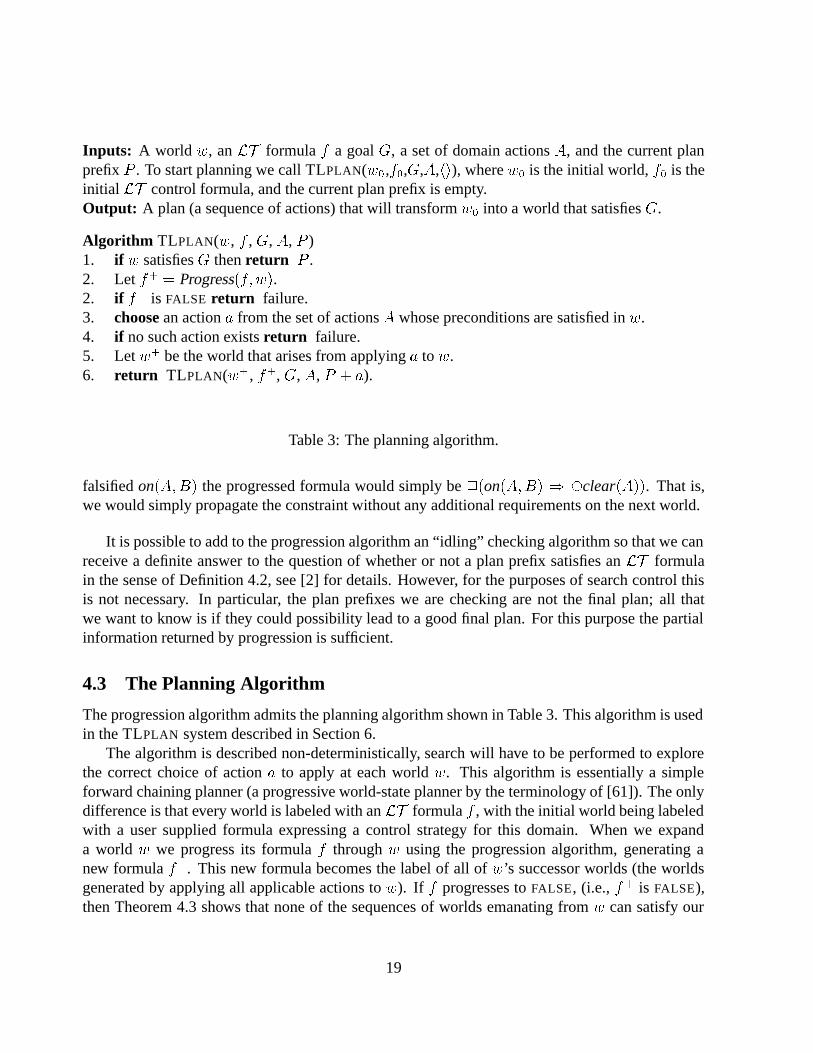
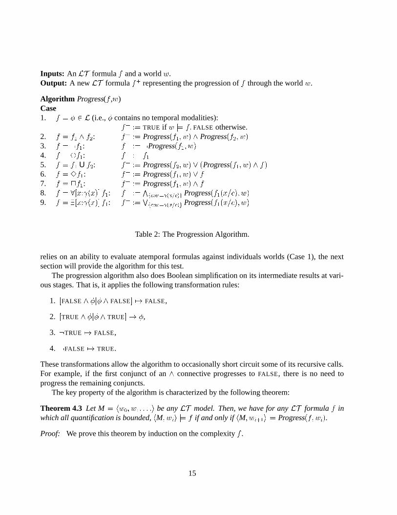
Inputs: A world �, an �� formula � a goal �, a set of domain actions �, and the current planprefix ! . To start planning we call TLPLAN(�� ,��,�,�,��), where �� is the initial world, �� is theinitial �� control formula, and the current plan prefix is empty.Output: A plan (a sequence of actions) that will transform �� into a world that satisfies �.

Algorithm TLPLAN(�, � , �, �, ! )1. if � satisfies � then return ! .2. Let �� Progress�� .2. if �� is FALSE return failure.3. choose an action � from the set of actions � whose preconditions are satisfied in �.4. if no such action exists return failure.5. Let �� be the world that arises from applying � to �.6. return TLPLAN(�� , ��, �, �, ! � �).

Table 3: The planning algorithm.

falsified on�� the progressed formula would simply be ��on�� clear��. That is,we would simply propagate the constraint without any additional requirements on the next world.

It is possible to add to the progression algorithm an “idling” checking algorithm so that we canreceive a definite answer to the question of whether or not a plan prefix satisfies an �� formulain the sense of Definition 4.2, see [2] for details. However, for the purposes of search control thisis not necessary. In particular, the plan prefixes we are checking are not the final plan; all thatwe want to know is if they could possibility lead to a good final plan. For this purpose the partialinformation returned by progression is sufficient.

4.3 The Planning Algorithm

The progression algorithm admits the planning algorithm shown in Table 3. This algorithm is usedin the TLPLAN system described in Section 6.

The algorithm is described non-deterministically, search will have to be performed to explorethe correct choice of action � to apply at each world �. This algorithm is essentially a simpleforward chaining planner (a progressive world-state planner by the terminology of [61]). The onlydifference is that every world is labeled with an �� formula � , with the initial world being labeledwith a user supplied formula expressing a control strategy for this domain. When we expanda world � we progress its formula � through � using the progression algorithm, generating anew formula ��. This new formula becomes the label of all of �’s successor worlds (the worldsgenerated by applying all applicable actions to �). If � progresses to FALSE, (i.e., �� is FALSE),then Theorem 4.3 shows that none of the sequences of worlds emanating from � can satisfy our

19

�� formula. Hence, we can immediately mark � as a dead-end in the search space and avoidexploring any of its successors.

5 Evaluating Atemporal Formulas in Individual Worlds

The previous section showed how we can checks plan prefixes to determine whether or not they(and thus all of their extensions) falsify an initial �� control formula. The process was provedto be sound but incomplete.16 The progression algorithm makes two assumptions: (1) each of theplan prefixes generated during search consist of sequences of first-order models, and (2) for anyformula � of �� containing no temporal modalities and any of the models in this sequence � wecan determine whether � satisfies � (case 1 of the algorithm).

In this section we will show that these assumptions are satisfied in the planning system weconstruct. First, as mentioned in the previous section, we represent each state in the plan as aSTRIPS database (with some extensions described below) and once the closed world assumption isemployed such databases are formally first-order models.17 Furthermore, our actions are modeledas performing database updates (this also follows the STRIPS model). Thus each action maps adatabase to a new database, i.e., a first-order model to a new first-order model. Hence, assumption(1) is trivially satisfied—each plan prefix consists of a sequence of first-order models.

To satisfy assumption (2) we simply need to specify an algorithm for evaluating atemporal ��formulas in these models (STRIPS databases). The formula evaluator algorithm is specified below.Once these two assumptions are satisfied we have that the progression algorithm is sound (in thesense of Observation 4.4).

The planning algorithm specified in Table 3 searches for plans that transforms the initial worldto a world satisfying the goal. It searches for this plan in the space of action sequences emanatingfrom the initial world and eliminating from that search space some set of plan prefixes. We havethe guarantee that any plan prefix eliminated from the search space has no extension satisfying theinitial �� formula.

The planning algorithm is trivially sound. That is, if a plan is found then that plan does in factcorrectly transform the initial state to a state satisfying the goal.18 The planning algorithm willbe complete, i.e., it will return a plan if one exists, when (1) the underlying search algorithm is

16Note that incompleteness does not pose a fundamental difficulty in our approach. Incompleteness means that wefail to prune away some of the invalid plan prefixes. The real issue, however, is whether or not we can prune away asufficient number of prefixes to make search more computationally feasible. In Section 7 we will provide extensiveevidence that we can.

17The pure STRIPS database is a finite first-order model. However the evaluator we describe below also has facilitiesto range variables over any finite set of integers and to evaluate numeric predicates and functions. This implies thatour system is actually implicitly dealing with infinite models. In particular, it is checking formulas over a first-ordermodel determined by the STRIPS database conjoined with the integers.

18Actions have a precise representation and a precise operational semantics (discussed below). The plan returnedwill be correct under specific interpretation of the action effects.

20

complete, and (2) whenever a plan exists a plan that does not falsify the initial�� formula exists.19

The formula evaluator checks the truth of formulas in individual worlds. Each world is rep-resented as an extended version of a STRIPS database. In particular, there are a distinguished setof predicates called the described predicates. Each world has a database containing all positiveground instances of the described predicates that hold in the world. The closed world assumptionis employed to derive the negations of ground atomic facts.

In addition to the described predicates a world might also include a set of described functions.These also are specified by a database, a database storing the value the described function has givenvarious arguments.

Actions map worlds to worlds, and their effects are ultimately specified as updates to the de-scribed predicates functions. This is the standard operational semantics for STRIPS actions, and infact these semantics are also applicable to ADL actions.20

Building on the database of described predicates we add defined predicates and functions.These are predicates and functions whose value is defined by a first-order formula. And we alsoadd computed predicates, functions and generators. These are mainly numeric predicates andfunctions that rely on computations performed by the underlying hardware. Thus the evaluatorcan evaluate complex atemporal formulas that involve symbols not appearing in the underlyingdatabase of described predicates.

The formula evaluator is given in Tables 4–6.The lowest level of the recursive algorithm is EvalTerm (Table 6) which is used to convert

complex first-order terms (containing functions and variables) into constants. Variables are easy,we simply look up their value in the current set of variable bindings. It is not hard to see that aslong as the top level formula passed to Eval contains no free variables (i.e., it is a sentence), the setof bindings will have a value for every variable by the time that variable must be evaluated.21

EvalTerm allows for three types of functions: computed, described and defined functions.Computed functions can invoke arbitrary computations on a collection of constant arguments (thearguments to the function are evaluated prior to being passed as arguments). The value of thefunction can depend on the current world or the function may be independent of the world. Forexample, it is possible to declare all of the standard arithmetic functions to be computed functions.Then when the evaluator encounters a term like #� � #� it first recursively evaluates #� and #� andthen invokes the standard addition function to compute their sum.

Every world contains a database of values for each described function, and these functionscan be evaluated by simple database lookup. The user must ensure that these function valuesare specified in the initial state and that the action descriptions properly update these values. Forexample, in the blocks world we could specify a function below such that below�� is equal tothe object that is below of block � in the current world (using the convention that the table is

19The first condition is a standard one for any algorithm that employs search. The second condition means that it isup to the user to specify sensible control knowledge, i.e., control knowledge that only eliminates redundant plans.

20ADL actions can have more complex first-order preconditions along with conditional add/deletes. However, theset of add/deletes each action generates is always a set of ground atomic facts.

21The quantifier clauses in Eval will set the variable values prior to their use.

21

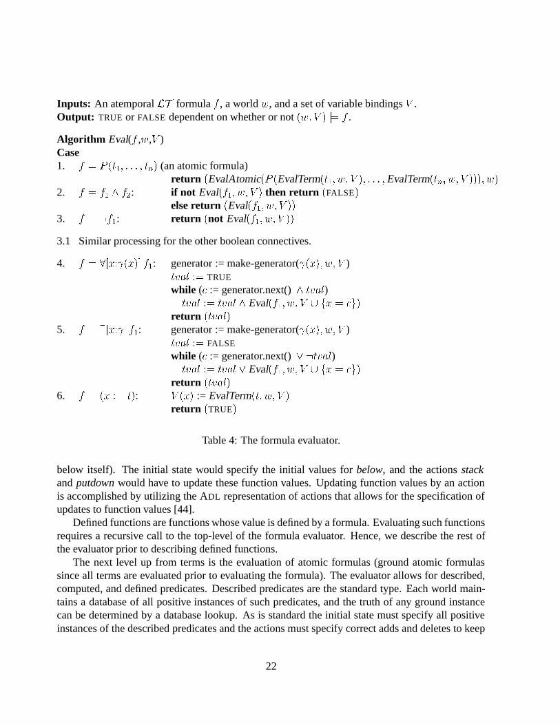
Inputs: An atemporal �� formula � , a world �, and a set of variable bindings � .Output: TRUE or FALSE dependent on whether or not �� .

Algorithm Eval(� ,�,� )Case1. � � ! �#�� #�� (an atomic formula)

return �EvalAtomic�! �EvalTerm�#�� EvalTerm�#�� 2. � � �� : if not Eval�� then return �FALSE�

else return �Eval�� 3. � � ��: return �not Eval��

3.1 Similar processing for the other boolean connectives.

4. � � �� : generator := make-generator(�� )#$�� TRUE

while (� := generator.next() � #$��)#$�� #$�� Eval��

return �#$��5. � � �� : generator := make-generator(�� )

#$�� FALSE

while (� := generator.next() � �#$��)#$�� #$�� Eval��

return �#$��6. � � �� #�: � �� := EvalTerm�#� ��

return �TRUE�

Table 4: The formula evaluator.

below itself). The initial state would specify the initial values for below, and the actions stackand putdown would have to update these function values. Updating function values by an actionis accomplished by utilizing the ADL representation of actions that allows for the specification ofupdates to function values [44].

Defined functions are functions whose value is defined by a formula. Evaluating such functionsrequires a recursive call to the top-level of the formula evaluator. Hence, we describe the rest ofthe evaluator prior to describing defined functions.

The next level up from terms is the evaluation of atomic formulas (ground atomic formulassince all terms are evaluated prior to evaluating the formula). The evaluator allows for described,computed, and defined predicates. Described predicates are the standard type. Each world main-tains a database of all positive instances of such predicates, and the truth of any ground instancecan be determined by a database lookup. As is standard the initial state must specify all positiveinstances of the described predicates and the actions must specify correct adds and deletes to keep

22

Inputs: An ground atomic formula ! �� and a world �.Output: TRUE or FALSE dependent on whether or not � �� ! �� .

Algorithm EvalAtomic(! �� ,�)Case1. ! is a described predicate:

return �lookup�! �� 2. ! is defined by a computed predicate:

return �! �� .3. ! is defined by the formula �:

Let �� be the arguments of �.return �Eval�� .

Table 5: Evaluating Atomic Formulas.

Inputs: A term #, a world �, and a set of variable bindings � .Output: A constant that is the value of # in the world �.

Algorithm EvalTerm(#,�,� )Case1. # � � where � is a variable:

return �� (i.e., return �’s binding)2. # � � where � is a constant:

return ��.3. # � ��#�� #�� where � is a described function:

return �lookup��EvalTerm�#�� EvalTerm�#�� .4. # � ��#�� #�� where � is a computed function:

return ��EvalTerm�#�� EvalTerm�#�� .5. # � ��#�� #�� where � is defined by the formula �:

For � � �� , let �� EvalTerm�#�� , �� be the arguments for �,and � � � � � ��

Eval�� return ��

Table 6: Evaluating Terms.

23

the database up to date.Computed predicates, like computed functions, can be used to invoke an arbitrary computation

(which in this case must return true or false). In this way we can include, e.g., arithmetic predicatesin our formulas. For example, weight�� % weight��, would be a legitimate formula given thatweight has been declared to a function. The formula evaluator would first evaluate the termsweight�� and weight�� prior to invoking the standard numeric comparison function to comparethe two values.

Finally, the most interesting type of predicate are the defined predicates. Like the defined func-tions these predicates are defined by first-order formulas. The predicate goodtower (defined inSection 3) is an example of a defined predicate. Defined predicates can be evaluated by simplyrecursively invoking the formula evaluator on the formula that defines the predicate (with appro-priate modifications to the set of bindings). The key feature is that this mechanism allows us towrite and evaluate recursively defined predicates. For example, we can define above to be thetransitive closure of on:

above�� on�� on�� above�� 22

At the top level the evaluator simply decomposes a formula into an appropriate set of atomicpredicate queries. The decomposition is determined by the semantics of the formula connectives.

Quantifiers are treated in a special manner. As previously mentioned our implementation uti-lizes bounded quantification. The formula specifying the quantifier bound is restricted: it can onlybe an atomic formula involving a described predicate, a goal atomic formula involving a describedpredicate, or a special computed function. Inside of the evaluator this is implemented by usingeach quantifier bound to construct a generator of instances over that bound. The function make-generator does this, and every time we send the returned generator a “next” message it returns thenext value for the variable. When a described predicate is used as a quantifier bound, a genera-tor over its instances is easy to construct given the world’s database: the generator simply returnsthe positive instances of that predicate contained in the database one by one. The implementationalso allows for computed generators which invoke arbitrary computations to return the sequenceof variable bindings.23 There is considerable generality in the implementation. N-ary predicatescan be used as generators. Such generators will bind tuples of variables; e.g., when evaluating theformula “�� on�� ” a generator of all pairs �� such that on�� holds in the currentworld will be constructed. The generators will also automatically take into account previouslybound variables. For example, when evaluating “��clear�� on�� ”, the outer gener-ator will successively bind � to each clear block and the inner generator will bind � to the singleblock that is below the block currently bound to �.

The last clause of the formula evaluator algorithm is used to deal with defined functions. Wewill discuss defined functions in Section 6.1.1.

22Of course the user has to write their recursively defined predicates in such a manner that the recursion terminates.The short circuiting of booleans and quantifiers (e.g., not evaluating the remaining disjunctions of an � once one ofthe disjunctions evaluates to true) is essential to this process.

23This is often useful when we want a quantified variable to range over a finite set of integers.

24

5.1 Evaluating GOAL Formulas

As mentioned in Section 2.2 the language utilized to express control formulas (and action precon-ditions in ADL formulas) includes a GOAL modality. In practice the user specifies the goal as somefirst-order formula . This generally means that if we can transform the initial state to any worldsatisfying we have found a solution to our problem. Hence, formally, the set of goal worlds �used to interpret GOAL formulas (see Section 2.2) should be taken to be the set of all first-ordermodels satisfying .

By the semantics for GOAL given in Section 2.2 and the above interpretation of the set of goalworlds, we have that GOAL�� is true iff �� . When the temporal control formula includesa goal modality (most control formulas do), then at every world when we progress the controlformula through that world we may have to invoke the evaluator to determine the truth GOAL

formulas, and hence the truth of �� for various �. To be of use in speeding up search wemust be able to efficiently evaluate GOAL formulas. In general, checking entailment (i.e., checking �� ) is not efficient.

When GOAL formulas are used in the control formulas (or as preconditions of ADL actions)we must enforce some restrictions in our implementation to ensure that they can be evaluatedefficiently. In particular, if GOAL formulas are to be used we require that the goal, , be specifiedas a list of ground atomic facts involving only described predicates, �&�� &��, and we restrictthe GOAL formulas that appear in the domain specification to be of the form GOAL�&� where &is an atomic formula involving a described predicate. Under these restrictions we can evaluateGOAL formulas efficiently with a simple lookup operation. Any set of ground atomic formulas hasa model that falsifies every atomic formula not in the set. Hence, under these restrictions GOAL�&�will be true if and only if & � . We can also efficiently utilize GOAL formulas in boundedquantification: all instances in the quantifier range must be instances that explicitly appear in .

Example 3 Let the goal be the set of ground atomic facts �ontable�� clear��.

� GOAL�ontable�� will evaluate to true.

� GOAL�ontable�� will evaluate to false.

� ��ontable�� GOAL�ontable�� will evaluate to true iff all the blocks on the table in thecurrent world are equal to �. The quantifier is evaluated in the current world �, and � issuccessively bound to every instance satisfying ontable in �. If � is bound to �, i.e., ifontable�� is true in �, then GOAL�ontable�� will evaluate to true. It will evaluate to falsefor every other binding. Hence, the formula will be true if there are no blocks on the table in� or if the only block on the table is �.

� ��GOAL�ontable�� ontable��, in this case the quantifier is evaluated in the goal world,and the only binding for � satisfying the bound is �� . Hence, this formula will evaluateto true in a world � iff � is on the table in �. There may be any number of other blocks onthe table in �.

25

5.2 Correctness of the Evaluator

Since the evaluator breaks down formulas according to their standard first-order semantics, it isnot difficult to see that if it evaluates atomic formulas and quantifier bounds correctly it will im-mediately follow that it evaluates all formulas correctly. First we deal with the quantifier bounds:

1. If the quantifier bound is GOAL�! �'��, then by the previous restrictions ! must be a de-scribed predicate. Furthermore, a binding '� for the sequence of variables '� satisfies thequantifier bound if and only if ! �'��'� � is in the list of ground atomic facts that specifies thegoal. Hence iterating over this list of facts will correctly evaluate the quantifier bound.

2. If the quantifier bound is ! �'�� where ! is a described predicate, then a binding '� for thevariables '� satisfies the quantifier bound if and only if ! �'��'� � is in the world’s database ofpositive ! instances. Iterating over the world’s database correctly evaluates the quantifierbound.

3. If the quantifier bound is a computed generator then whatever function the user supplies itmust generate some sequence of bindings given the current world and current set of bindings.We take this sequence to be the definition of the set of satisfying instances of the quantifierbound. Thus by definition computed generators are correctly evaluated.24

Atomic formulas require using EvalTerm to evaluate the terms they contain:

1. If the term is a variable, then its value is its the current binding which will have been set bythe generator for the quantifier bound. It has been shown above that the generators operateset these bindings correctly.

2. Constants are their own value, thus EvalTerm correctly evaluates such terms.

3. If the term is a described function, then the STRIPS database contains all of the values of thatfunction and a simple lookup will correctly evaluate such terms.

4. If the term is a computed or defined function then we take the value returned to define thefunction. (The operational semantics of defined functions is described in the next section).Hence, such terms are evaluated correctly by definition.

Finally, we have the atomic formulas.24The system cannot ensure the user supplied generator function implements what the user intended. Rather all it

can do is provide a specific semantics as to how the output of that function will be used, and ensure that it correctlyimplements those semantics. This is the same approach as that taken by, e.g., programming languages compilers. Thelanguage specifies a specific semantics for every language construct and the compiler is correct if it correctly mapsprograms to this specified semantics. Whether or not the program implements what the user intended is a separatematter.

26

SearchEngine

State ExpanderFormula

Progressor

FormulaEvaluator

Goal Tester

Figure 2: The TLPLAN system

1. If the atomic formula involves a described predicate, then the STRIPS database contains allpositive instances of the predicate. Such predicates can be evaluated by a simple databaselookup procedure.

2. If the atomic formula involves a defined predicate then its evaluation is can be shown tobe correct by induction (with the base case being the atomic predicates that are not definedpredicates).25

3. If the atomic formula is a computed predicate, then again we take the value returned by thecomputation to define the predicate.

6 The TLPLAN System

We have constructed a planning system called the TLPLAN system that utilizes the planning algo-rithm shown in Table 3. In this section we describe the system and supply some final details aboutthe design of the system.

TLPLAN is a very simple system, as the diagram of its components shown in Figure 2 demon-strates. The distinct components of the system are:

25There is a subtlety when the defined predicate is recursive. In this case we need fixpoints to give a precisesemantics to the predicate. It goes beyond the scope of this paper to supply such semantics, but many approaches tothis problem have been developed by those concerned with providing semantics to database queries (which can berecursive), e.g., see [58].

27

� A search engine which implements a range of search algorithms.

� A goal tester that is called by the search engine to determine if it has reached a goal world.The goal tester in turn calls the formula evaluator to implement this test.

� A state expander that is called by the search engine to find all the successors of a world. Thestate expander in turn calls the formula evaluator to determine the actions that are applicableat a world. It also calls the formula progressor to determine the formula label of these newworlds.

� A formula progressor which implements the progression algorithm shown in Table 2. Theprogression algorithm uses the formula evaluator to realize line 1 of the algorithm.

� A formula evaluator which implements the algorithm shown in Tables 4–6.

Forward-chaining planners like TLPLAN are inherently simple. Nevertheless, is it worth point-ing out that all of the functionality needed in such a planner can be implemented using the eval-uator. As Figure 2 shows, this is the design used by TLPLAN. A properly designed formulaevaluator also provides considerable additional flexibility and expressiveness to the system, andunderstanding its operation provides insights into the worst case complexity of the planner’s basicoperations.

6.1 Utilizing the Evaluator’s Operational Semantics

It was shown in the previous section that the formula evaluator correctly determines the truth ofany atemporal �� formula. However, there is another way to view of the evaluator: the evaluatorcan be viewed as being an interpreter for a language, a language whose syntactic structure is that ofthe atemporal component of �� . When viewed as an interpreter the evaluator has an operationalsemantics [28] that is precisely specified by the algorithm given in Tables 4–6.

In particular, when the evaluator is given a formula to evaluate it will perform a precise se-quence of computations determined by the syntactic structure of the formula and the properties ofthe world against which the formula is being evaluated. For example, say we evaluate the formulaon�� on�� in a world � in which on�� holds and on�� does not. The evaluatorwill perform the following computations:

1. It will evaluate on�� in �. This will evaluate to TRUE.

2. It will then evaluate on�� in �. This will evaluate to FALSE.

3. It will return FALSE.

On the other hand if we evaluate the formula on��on�� the evaluator will never performthe computation of evaluating on�� in �.

28

This behaviour stems from the fact that the evaluator utilizes early termination of booleanconnectives and quantifiers. From the point of view of correctness early termination makes nodifference; the evaluator returns the same value no matter how the formula is written. However,early termination can be a very useful control flow mechanism when we add additional computedpredicates.

Computed predicates and functions invoke a user defined computation in order to return a valueto the evaluator. Great economy in the implementation can be achieved by taking advantage of thisfact. In particular, much of the implementation is realized by simply supplying an additional set ofcomputed predicates and functions. These predicates and functions return specific values, but theyare mainly designed to invoke useful computation when they are evaluated.

Printing is a good example. The system defines a computed “print” predicate (taking an arbi-trary number of arguments). This predicate always returns true as its truth value, thus any formulacontaining print can always be rewritten by replacing all instances of print with TRUE. However,when the evaluator evaluates the print predicate the computation it invokes generates I/O as aside effect. Such predicates have a trivial declarative semantics (usually they are equivalent to thepropositional constant TRUE). Their effects are determined by the computation they invoke whenevaluated and the evaluator’s operational semantics (which determines under what conditions theywill be invoked).

For example, in the world � used in the example above the formula

on�� print�“on�� holds!”� � on�� print�“on�� holds!”�

will evaluate to FALSE just as before, but its evaluation will print out the string “on�� holds!”as a side effect, while the formula

on�� print�“on�� holds!”� � on�� print�“on�� holds!”�

will also return FALSE but will not generate any I/O since its evaluation will terminate prior to thefirst print statement being evaluated.

This example shows that viewing the evaluator as an interpreter makes formula evaluation moresyntax dependent, but in no way affects the correctness of the final value it returns.26 Despite thisdrawback, by utilizing the evaluator as an interpreter we can implement many of the remainingcomponents of the planner quite easily. We discuss these components next.

6.1.1 Defined Functions

The operational semantics of the evaluator provides a mechanism that allows the user to specifydefined functions. Such functions are handled by the last clause of the formula evaluator algorithm(Table 4).

26It should also be noted that if we are thinking of the evaluator as an interpreter it should not be too surprising that,e.g., the order of the conjunctions in a formula make a difference. The order of statements makes a difference in mostprogramming languages.

29

Consider a function depth�� that returns the depth of a block �, where clear blocks have depthzero. Such a function can be computed by evaluating the following formula:

depth��

clear�� depth �� on�� depth �� depth��

That is, the depth of � is zero if � is clear, otherwise there must exist another block � that is on topof � and then the depth of � is one more than the depth of �.

Formulas defining functions utilize the computed assignment predicate “:=”. This predicate ishandled by the last clause of the evaluator’s algorithm. Assignment always returns TRUE and as aside effect it sets the binding of a variable to be equal to the value of the term on the left hand side.

Defined functions use the convention of assigning values to the function’s name as a shorthandfor setting the return value. The value of the function is the last value assigned to its name. In-ternally, defined functions are handled by adding the function name as a new unassigned variableto the set of variable bindings (see clause 5 of the EvalTerm algorithm Table 6). We then evaluatethe formula defining the function using this augmented set of variable bindings. When the evalua-tor encounters an assignment “predicate” like depth �� it modifies the binding of that variable.Thus, after the evaluator has processed the defining formula, the function’s name variable has beenset to a value, and that value is returned as the function’s value. This simple mechanism addsconsiderable flexibility when defining a planning domain.27

It should also be noted that this formula defining depth has been written so that its interpretationby the evaluator will yield the correct value for depth. In particular, the consequent of each of theimplications (i.e., the assignments) will only be evaluated when the antecedent evaluates to TRUE.

6.1.2 The Progression Algorithm

As shown in Table 2 case one of the progression algorithm needs to evaluate whether or not varioussubformulas holds in the current world. This is accomplished by calling the formula evaluator. Auseful illustration of the working of the progression algorithm and the formula evaluator is providedby the following example.

Example 4 Consider a control formula from the blocks world:

�

�� ontable�� GOAL�on�� holding��

�� (4)

This formula asserts that a good plan will never pickup a block � from the table if that block is notrequired to be on another block �. Say that we wish to progress this formula through a world � inwhich the �ontable��, ontable�(��, and �clear��, clear�(��, are the set of ontable and clear facts

27Our implementation extends this mechanism to allow defined functions (and predicates) to have local variablesthat can be assigned to. Local variables are not essential, but they can speedup certain computations.

30

that hold in �. Further, say that the goal is specified by the set ��(� ��. On encountering the �modality the progressor will compute the progression of

�� ontable�� GOAL�on�� holding�� (5)

and then return the conjunction of the result and the original formula 4 (case 7 of Table 2).To progress the subformula the evaluator will be called to make a generator of the instances of

clear�� that hold in �, and for each of these instances the progressor will progress the subformula

ontable�� GOAL�on�� holding�� (6)

The first call to this generator will return �� . Using this binding subsequent calls to theevaluator will return true for ontable��, and then true for ��GOAL�on�� , as there are noinstantiations for � that satisfy on�� in the goal world. This terminates the progression of theantecedent of the implication. Since the antecedent is true the progressor is forced to progress theconsequent of the implication ��holding��. The end result of the first instantiation for � is theprogressed formula �holding��.

The next call to the top level generator returns the binding �� (�. Under this new bindingontable�� evaluates to true but ��GOAL�on�� evaluates to false, as the binding �� satisfies the existential. Thus the conjunction evaluates to false, and the entire implication thenprogresses to true.

The final result is the formula

�holding��

�� ontable�� GOAL�on�� holding��

��

which says that in the subsequent state we should not be holding � (remember that the progressedformula is used to label all of the successor worlds of �).

6.1.3 Implementing the Operators

Actions are specified as either STRIPS or ADL operators. When we instantiate the parameters ofthe operators we obtain an action instance with instantiated precondition, add, and delete clauses.An action can be applied to the current world if its instantiated precondition is satisfied in theworld.

It is easy to use the formula evaluator to determine if an action precondition is satisfied in thecurrent world. However, we can go further than this. By utilizing the evaluator as an interpreter andadding some appropriate computed predicates, we can use the formula evaluator to fully implementthe operators.

This process is best illustrated by an example. Consider the STRIPS operator unstack specifiedin Table 1. Its precondition list is �on�� clear�� handempty�, its add list is �holding�� clear��,and its delete list is �on�� clear�� handempty�. We can represent this operator as a formula.

31

When this formula is evaluated in the current world it will, as a side effect of some of its com-puted predicates, correctly construct all of the successor worlds that could be generated by variousexecutable instances of the operator. The formula for unstack is

handempty ��clear�� on�� MakeNewWorld� Del�on�� Del�� Del�)��*+#�� Add�holding�� Add�clear��

When this formula is evaluated in the current world the first thing that is done by the evaluator isto test if handempty is true. If it is not then no instance of unstack is applicable and no furthercomputation is necessary. Then the quantified subformulas are evaluated. The variables � and �will be instantiated to objects that satisfy the preconditions of the operator; i.e., by representing theoperator’s parameters as quantified variables we can use the standard processing of quantifiers tofind all executable actions. The new computed-predicates we need are “MakeNewWorld”, “Add”,and “Del”. “MakeNewWorld”, generates a new copy of the current world, and “Add” and “Del”modify the databases that describe the instances of the various predicates that hold in that copy.28

(All of these predicates evaluate to TRUE in every world.) That is, by “evaluating” these predicatesthe world generated by applying the current action (given by the current bindings of � and �) iscomputed. It is not difficult to see that any STRIPS operator can be translated into a formula of thisform.29

Using the same mechanism it is also easy to handle ADL operators (in their full generality).ADL operators can take arbitrary first-order formulas as their preconditions, and have conditionaladd and delete lists. Furthermore, these operators can update function values. Every ADL operatoris converted into a formula with the following form

�'��'�� MakeNewWorld� �'��'�� '�� Add�,��'�� '��

...� �'��'�� '�� Del�,��'�� '��

The formula ��'�� is the precondition of the operator. It contains a vector of free variables '�. Everinstantiation of '� that makes ��'�� true in the current world specifies a single executable action. Forevery action all of the conditional updates ��'�� '�� are activated. Each of these conditional updatescan potentially add or delete many instances of a predicate ,�. That is, for a fixed instantiation of'� there may be many instantiations of '�� that satisfy the conditional update formula ��'�� '��. The

28Add and Del are syntactically unusual in that they actually take atomic formulas as arguments. If we wanted tobe pedantic we would say that they are computed modalities not computed predicates.

29An interesting point is that since we convert operator into formulas universally quantified by the operator param-eters, there is never any need to do unification. In particular, the unification algorithm plays no role in the TLPLAN

system.

32

action instance will add or delete an instance of the predicate ,� for every distinct instantiation of'�� that satisfies ��'�� '�� (in the current world).

Function updates are handled in a uniform manner using equality as the predicate. That is, aterm like Add�� will update the function � so that its value on � is equal to � (i.e., thecurrent binding of �). Since functions have unique values, the add of a function value automaticallydeletes the old value.

The actual ADL and STRIPS operators are specified using a sightly more standard syntax andthen translated to the above form. Once in this form we can make direct use of the formulaevaluator to apply these operators to the current world.

6.2 Testing Goal Achievement

As discussed above the goal is usually specified as a list of ground atomic facts �,�� ,��. Totest if a world � satisfies the goal we evaluate the conjunction ,�� ,� in�. Thus the evaluatoris used directly to test for goal achievement.

As we will point out below checking arbitrary formulas against a world is efficient. So we couldin principle give the planner goals, , expressed as complex first-order formulas. The planner canperform search and at every world evaluate the formula in the current world to see if the goalhas been achieved. This would produce a planner capable of generating plans for achieving, e.g.,disjunctive or quantified goals, and in fact TLPLAN can be configured to accept an arbitrary first-order formula as its goal.

The only problem with general goals of this form is that if � is an arbitrary formula, thenchecking if GOAL�� holds for various � (i.e., checking if �� ) becomes hard (it requirestheorem proving). For this reason TLPLAN does not accept formulas as goals when the domainutilizes GOAL formulas.

6.3 Complexity of the Planner’s Components

The domain specifications accepted by TLPLAN are sufficiently general so that it is quite possibleto write specifications which cause the planner’s basic operations to be intractable. Nevertheless,we have found that in practice the planner is very efficient in its basic operations. Since the formulaevaluator is at the heart of the system, we start by examining its complexity.

6.3.1 Evaluating Formulas

Evaluating a formula is usually very efficient. In particular, if � is a quantifier free formula inwhich no computed or defined functions or predicates appear, then evaluating � has complexitylinear in the length of �. The basic set of described functions and predicates in � can be evaluatedin near constant time,30 as can the boolean connectives.

30Using indexing or hashing techniques we can perform these database lookups in near constant time. In the actualimplementation, however, we found that a simpler albeit log-time binary tree representation of the world databases

33

When � contains computed predicates or functions nothing can be said in general about theperformance of the evaluator, since such predicates and functions can invoke arbitrary computa-tions. In our test domains have we found computed predicates and functions to be very useful, buthave never found a need to define ones that were particularly expensive to compute.

Once we allow � to contain quantifiers, formula evaluation becomes PSPACE-complete. Thisis easily shown by reduction to the quantified boolean formula problem, which is known to bePSPACE-complete [29]. A quantified boolean formula is a formula of the form

-��-�� -��

where each -� is either a universal or existential quantifier, each �� is a boolean variable, and �is a boolean expression involving the ��. The problem is to determine whether or not this formulais true. For example, �� is a true formula, as no matter what value � takes there exists avalue for � (namely TRUE) that makes the formula � � � true. On the other hand, �� isfalse, as the values � � FALSE and � � FALSE make � � � false.

Consider a world � in which we have two predicates, a type predicate ��, and a “truth”predicate . . The only positive instances of these two predicates true in � are ��TRUE�,��FALSE�, and . �TRUE�. We can convert any quantified boolean formula � to a first-orderformula by replacing each universal (existential) quantifier �� (��) in � by the bounded quan-tification �� (�� ). Similarly in �’s boolean expression � �� wereplace every variable �� by the atomic formula . ��. For example, the quantified boolean for-mula �� becomes the formula �� . �� . ��. It is not difficultto see that the converted formula evaluates to true in the world � if and only if the original quan-tified boolean formula was true. This shows that evaluating quantified formulas is PSPACE-hard.That the algorithm is in PSPACE is also an easy observation: although we may need to test manydifferent sets of bindings for the quantified variables, at any stage the algorithm need store onlyone set of bindings.

This observation indicates that we can easily write quantified formulas that would be intractablefor the formula evaluator. However, in practice things are not as bad. Let / be the total numberof objects in the domain, and let the deepest level of quantifier nesting in the formula � be �.Then at worst, evaluating � will take time 0�/ ��. The PSPACE result holds because we can writeformulas with � nested quantifiers in length 0��. Every increase in quantifier nesting adds to thesize of the exponent. In practice we have rarely found a need to nest quantifier more than 3 deep,in which case evaluating these formulas remains polynomial in complexity, 0�/ � in fact. Theformula evaluator has not been a performance bottleneck in any of our test domains.

There is one area, however, where we must be careful about evaluating quantified formulas. Asmentioned above, we determine the set of actions that can be executed in the current world by eval-uating a formula in which the operator’s parameters are converted into quantified variables. Theway in which we convert the operator description into a quantified formula can make a significantdifference in the planner’s performance. This is best illustrated by an example.

gives excellent performance.

34

Consider the formula that encodes the unstack operator (previously given in Section 6.1.3):

handempty ��clear�� on�� MakeNewWorld� Del�on� �� Del�clear� �� Del�)��*+#�� Add�holding� �� Add�clear� ��

An alternate encoding of this operator would be the formula

��clear�� on�� handempty MakeNewWorld� Del�on� �� Del�clear� �� Del�)��*+#�� Add�holding� �� Add�clear� ��

This formula is logically equivalent, yet far less efficient. In worlds where handempty is false, theevaluator can immediately recognize that no instance of unstack is applicable when using the firstformula. When using the second formula, however, the evaluator must iterate over every pair ofobject �, � such that clear�� and on�� . For every iteration, the evaluation of handempty willfail to produce an applicable instance of unstack . Thus the first formula evaluates in constant time,while the second takes 0�/ �� where / is the number of blocks in the domain.

Since the action formulas must be evaluated at every world in the forward chaining searchsuch differences can have a significant impact on the planner’s efficiency. The issues involved inchoosing which of the logically equivalent formulas to generate when converting an action intoa formula (e.g., how to choose the ordering of two adjacent universal quantifiers) are essentiallythe same as the issues that arise in the area of query optimization in databases. And needless tosay there is a considerable body of work in this area that could be applied to this problem. Ourimplementation employs some simple heuristics along these lines when it converts operators intoformulas.

The final issue that arises when examining the complexity of the formula evaluator is that ofdefined predicates. As mentioned above, defined predicates invoke the evaluator on the formulathat defines the predicate. This formula can be recursive. This means that a single predicateinstance in a formula may end up invoking considerable additional computation as the evaluatorrecurses over its definition. Again it is easy to see that there can be no a-priori bound on thecomplexity of this process. However, as in the previous cases we have not found this to be aparticular problem in our test domains.

6.3.2 State Expansion and Goal Testing

As described above, state expansion (i.e., finding and applying the set of actions that can be appliedto the current world) and testing for goal achievement both involve utilizing the formula evaluator.Hence, the complexity of these two components is determined by the complexity of the formulaevaluator.

35

6.3.3 Progressing Formulas

The process of progressing formulas is another area where expensive computations might be in-voked. As can be seen from Table 2, the progression algorithm is generally quite efficient. Inparticular, except for quantification the process is essentially linear in the size of the input for-mula.31 With quantification, however, it is possible to specify a short formula that takes a longtime to progress.

The difficulty with progression lies not so much with progressing a formula once, but ratherwith the repeated progression of a formula through a sequence of worlds. During planning when weexplore a sequence of states �� we have to progress the original temporal control formula� times, one through every world��. The formula might grow in length with each progression, andif we are not careful this can lead to excessive space and time requirements. For example, considerthe progression of the temporal formula

! �� U �! �(� U �! �� U-��

through a world � in which ! ��, ! �(�, and ! �� all hold, but -�� does not. The progressionalgorithm yields the new formula

! �� U-�� ! �(� U �! �� U-�� ! �� U �! �(� U �! �� U-��

Formulas of this form progress to formulas that have grown quadratically in size. Furthermore, theformula grows even longer as we progress it through multiple worlds.

The key to an efficient implementation of the progression algorithm is to realize that the pro-gressed formula has many subformulas in common with the original formula. Hence, considerableefficiency can be gained by sharing these subformulas. In fact, in the above example, if we sharesubstructures the progressed formula only requires us to store two new top level “�” connec-tives. Structure sharing is a well known technique in automated theorem provers, and we haveemployed similar techniques in our implementation. In addition to space efficiency structure shar-ing also yields computational efficiency. Progression distributes over the logical connectives (e.g.,Progress�� Progress�� Progress��). Hence, once we have computed the progressionof subformula that progression can be spliced in where ever the subformula appears, i.e., we needonly compute the progression of a subformula once. In the above example, if we have to progressthe new formula one more time we only need to progress the subformula “! ��U-��” once, eventhough it appears three times in the formula.

With these structure sharing techniques it is quantification that has the main impact on theefficiency of progression in practice. Consider the formula

��object��! ��31Progression also invokes the evaluator on atemporal subformulas, and, as noted above, this also has the potential

to be intractable.

36

If we progress this formula through a world � in which no object satisfies ! and object��,object�(�, and object�� all hold, then we get the new formula

��object��! ��! �� ! �(� ��! ��

Since the progression algorithm deals with quantifiers by expanding each of the particular in-stances, we see that the progression of the formula grows in length by a factor determined by thenumber of objects satisfying object that currently fail to satisfy ! . When there are � nested quan-tifiers the progressed formula can be of length 0�/ ��, where / is the number of objects in thedomain. This behaviour is analogous to the behaviour of the formula evaluator in the face of nestedquantification. However, as in that case, we have rarely found a need to nest quantifiers more than3 deep in our temporal control formulas.

Furthermore, many natural control formulas do not continue to grow continually length. Con-sider, for example, the control formula specified for the blocks world (Formula 3). This formulawhen progressed through any world will generate a collection of conditions that must hold in thenext world. In particular, there will be a collection of good towers that must be preserved, a collec-tion of bad towers that nothing can be placed on top of, and a collection of blocks that cannot beheld in the next state. These conditions are all checked and discharged in the next world. Thus, thelength of the control formula grows and shrinks, but never grows monotonically as we progress itthrough a sequence of worlds.

In summary, TLPLAN allows for very expressive domain specifications. It is sufficiently ex-pressive that it is quite possible to express domains in which the basic operations of the plannerbecome intractable. In practice, however, we have have found the planner’s expressiveness to bea boon not a bane. It allows for a easy specification of domains and the potential of intractabilityof the basic operations has not been a major issue so far. Note that the tractability of planningin any domain is a separate issue from the tractability of the planner’s basic operations. That is,although tractability of the basic operations is a necessary condition for tractable planning, it is byno means sufficient. Our empirical results (Section 7), however, do show that with the right controlknowledge TLPLAN can plan very effectively in many test domains.

7 Empirical Results

We have implemented a range of test domains to determine how easy it is specify control informa-tion in our formalism and how effective that information is in controlling planning search.

In our empirical tests we ran TLPLAN on a Pentium Pro 200MHz machine with 128MB ofRAM. This amount of memory was more than sufficient for TLPLAN in all of the tests. We alsoran various tests using the BLACKBOX [33], IPP [37], SATPLAN [32], PRODIGY [59], and UCPOP

[7] systems.BLACKBOX and SATPLAN are similar systems both of which encode planning problems as sat-

isfiability problems. SATPLAN uses a different encoding that can be more efficient, while BLACK-

37

BOX employs various simplification steps interleaved with its generation of the encodings. IPP isbased on the GRAPHPLAN [13] algorithm, but has been optimized in various ways and extendedto handle a subset of the ADL language. BLACKBOX and IPP are both state of the art planningsystems. They were the best performers in the AIPS’98 planning competition [1] and are bothcoded in C (as is TLPLAN). However both of these systems have tremendous appetites for mem-ory, and so we ran them on a SUN Ultra 2 296MHz machine with 256MB of RAM. This still wasnot sufficient memory for these systems, but we were careful in recording the cpu time used so asnot to count the time taken by swapping. Furthermore, fairly clear trends were already establishedby time the problems became large enough to start excessive thrashing. It should be noted howeverthat BLACKBOX’s and IPP’s high memory consumption is not something that should be ignored.Space can be as much of a limiting resources as time, and in some cases more so.

The older systems UCPOP and PRODIGY are coded in lisp, and so we ran them on a 196MHzSUN Ultra 2 that had support for lisp. However, the performance difference between these systemsand the others was so great that recoding in C and running of the faster machine would not havehelped much.

7.1 Blocks World

TLPLAN’s performance with the three different control formulas, (Formulas 1–3 given in Sec-tion 3), using depth-first search is shown in Figure 3. Each (�,�) data point represents the averagetime � taken to solve 10 randomly generated blocks world problems involving � blocks. In par-ticular, for each value of � we generated a random initial configuration of blocks and asked theplanner to transform this configuration to a randomly generated goal configuration.

The graph also shows the time taken by the planner when it employed breadth-first searchusing the final control strategy, and the time taken by blind breadth-first search. (Blind breath-firstoutperforms blind depth-first search in this domain). The data shows that control information actsincrementally, as we add more clauses to the control formula the planner is able to search moreefficiently by pruning more paths from the search space. It also shows just how effective the searchcontrol can be—TLPLAN is able to solve 100 blocks problems in about 8 minutes when usingdepth-first search and control strategy 3 (compare this with the performance of other state of theart planners shown in Fig. 5).

The data generated by the breadth-first search represent the time to find optimal plans.32 Thedata shows that control strategies can be a considerable aid in solving the optimization problemas well. Using control 3 TLPLAN is able to generate optimal plans for 18 block problems inreasonable time (42 seconds on average), while without control optimal 6 block problems areabout the limit (7 blocks take more than 1000 seconds). Nevertheless, generating optimal plans inthe blocks world is known to be NP-hard [26], and even the control strategies are insufficient forgenerating optimal solutions to all of the 19 blocks problems.

32A control strategy could eliminate optimal plans from the search space: if no optimal plan satisfies the controlstrategy the strategy will stop the planner from finding an optimal plans. However, it is easy to show that no optimalplan is eliminated by these blocks world control strategies.

38

In the blocks world depth-first search can always find a solution,33 but the solution may bevery long. Figure 4 shows the length of the plan found by the planner using the different controlstrategies. (Control 2 generates identical plans to Control 3, but takes longer). The data alsoshows that the plans generated by control 3 are quite high quality plans (measuring quality byplan length). They are only slightly longer then the optimal length plans. In fact, it can be showthat the plans generated by control 3 (and control 2) are no longer than 2 times the length of theoptimal plan.34 Furthermore, TLPLAN is able to generate plans using these strategies withoutbacktracking. Hence, these control strategies yield a polynomial-time blocks world planner with areasonable plan quality guarantee.

The blocks world remains a very difficult domain for current domain-independent planners.Figure 5 shows how a range of the other planning systems perform in the blocks world.

7.2 Briefcase World

The briefcase world is a very simple domain invented by Pednault to illustrate his ADL actionrepresentation [44]. In this domain we have a briefcase that can be moved between differentlocations. Objects can be put in and taken out of the briefcase, and when they are in the briefcasethey are moved with it. There is a simple and intuitive search control formula that can be written forthis domain. What is most interesting however, is that the ideas in this search control appear almostunchanged in another popular test domain, the logistics domain (see below). We have found thatthere are many “meta-level” strategies that are applicable across different domains under slightlydifferent concrete realizations.

The operators in this domain are given in Table 7.

(def-adl-operator (MOVE-BRIEFCASE ?to) (def-adl-operator (PUT-IN ?x)(pre (pre

(?from) (at briefcase ?from) (?loc) (at briefcase ?loc)(?to) (location ?to) (?x) (at ?x ?loc)

(not (= ?from ?to))) (and (not (= briefcase ?x))(add (at briefcase ?to)) (not (in-briefcase ?x))))(del (at briefcase ?from)) (add (in-briefcase ?x)))(forall (?z) (in-briefcase ?z)(and (def-strips-operator (TAKE-OUT ?x)

(add (at ?z ?to)) (pre (in-briefcase ?x))(del (at ?z ?from))))) (del (in-briefcase ?x)))

Table 7: The Briefcase World Operators.

The operators are given in TLPLAN’s input language, which is basically first-order logic writ-ten in a lisp syntax. Two types of operators are accepted, standard STRIPS operators and ADL

33In the blocks world every state is reachable from every other state, so any cycle-free depth-first path must eventu-ally reach the goal.

34Control 3 encodes a strategy very similar to the reactive strategy given by Selman in [49], and he proves that thisreactive strategy never exceeds the optimal by more than a factor of 2.

39

0

50

100

150

200

250

300

350

400

450

500

0 10 20 30 40 50 60 70 80 90 100

Sec

onds

CP

U T

ime

Number of Blocks

Control 1 fails on 1 problem of size 11

No Control (breadth-first)Control 1Control 2Control 3

Control 3 (breadth-first)

Figure 3: Performance of TLPLAN search control in the Blocks world

40

1

10

100

1000

10000

0 10 20 30 40 50 60 70 80 90 100

Pla

n L

engt

h

Number of Blocks

Control 1 generates very long plans (note log scale)

Control 3 generates near optimal plans

Control 3 (breadth-first), BlackBox, and IPP generate optimal plans in this domain

Control 1Control 3

Control 3 (breadth-first)

Figure 4: Length of plans generated by TLPLAN in the Blocks world

41

0

50

100

150

200

250

300

350

400

450

500

2 4 6 8 10 12

Sec

onds

CP

U T

ime

Number of Blocks

UCPOP fails on all problems of size 6

IPP fails on 2 problems of size 11 and 12exceeds 1GB RAM on problems of size 13

SatPlan fails on 3 problems of size 10

BlackBox fails on 1 problem of size 10

IPPUCPOPSatPlan

BlackBox

Figure 5: Performance of other planners in the Blocks world

42

operators. Each consists of a sequence of clauses. The first clause is the name of the operator, andit may contain variables (e.g., ?x in the “take-out” operator).35

Taking something out of the briefcase can be specified as a simple STRIPS-style operator witha precondition, an add and a delete list. Each of these is a list of atomic predicates. The other twooperators, “move-briefcase” and “put-in” are specified as ADL-style operators.

ADL operators are specified by using a precondition clause that acts exactly like a quanti-fier clause. In particular, all of the variables in the clause must be specified first (as with allquantifiers). All quantification is bounded quantification, so we must specify a quantifier boundfor each of these variables. For example, for the “put-in” operator, ?loc ranges over all of thelocations the briefcase is at (there is in fact only one such location), while ?x ranges over allobjects that are at that location. Note that ?x is scoped by ?loc. Thus for each binding of?loc we compute a distinct range of bindings for ?x. After the variable bindings the precondi-tion can include an additional formula that can test the variable bindings and any other requiredfeatures of the current world. Note that this formula can be an arbitrary first-order formula, itmay include disjunction, other quantifiers, etc.36. For example, the operator “put-in” includesthe formula (and (not (= briefcase ?x)) (not (in-briefcase ?x))). Eachbinding of the precondition variables that satisfies the precondition formula generates a unique in-stance of the operator (an operator instance is also called an action). The bindings of the variablesappearing in the operator name are then used to give each action a unique name.37

Subsequent to the precondition formula come a sequence of clauses. These clauses are allscoped by the precondition’s variables (and thus may access their bindings) and they are eachindividually evaluated by the formula evaluator (see Section 6). During evaluation any “add” or“del” clause always evaluates to TRUE and has the side-effect of modifying the new world. Thecurrent state of the world as well as the manner in which the evaluator works (i.e., its rules for theearly termination of formula evaluation) precisely specifies the set of adds and deletes generatedby this instance of the operator.

Thus, in the “move-briefcase” action, we add the briefcase’s new location and delete its old lo-cation.38 Then a universal quantifier is used to successively bind ?z to all objects that are currentlyin the briefcase. For each such binding the body of the universal is evaluated. The body of theuniversal is a conjunction, so we evaluate the first add. All terms in the add clause are evaluated,and in this case the variables ?z and ?to evaluate to the objects they are currently bound to (seeTable 6). This results in a ground atomic fact being added to the world database.39 The add clausealways evaluates to TRUE, so the evaluator moves on to evaluate the second conjunct, the delete.

35Variables in TLPLAN are always prefixed with “?”.36Other planning systems that accept ADL specified actions, e.g., UCPOP and IPP, accept only a restricted subset

of the ADL specification. For example, disjunctive preconditions are usually not allowed.37Every operator instance need not have a unique name. Sometimes it is useful to treat different instances as being

the same action.38TLPLAN internally reorders the adds and deletes so that all deletes are executed prior to any adds.39All of the predicates and functions that appear inside of an add or a delete must be described symbols, as only

these can be directly updated.

43

The end result is that we update the locations of the briefcase and all the objects in the briefcase.Search control formulas for this domain are easy to write. They embody the following obvious

ideas:

1. Don’t move the briefcase from its current location if there is an object that needs to be takenout or put into the briefcase.

2. Don’t take an object out of the briefcase if the briefcase is not at the object’s goal location.

3. Don’t put objects that don’t need to be moved into the briefcase.

4. Don’t move the briefcase to an irrelevant location. In this domain a location is irrelevant ifthere is no object to be picked up there, there is no object in the briefcase that needs to bedropped off there, and it is not a goal to move the briefcase to that location.

The control formula given in Table 9 realizes these rules. We give the formula exactly as it isinput to the planner. The planner can take as control input any formula of �� . The only differencesare that (1) we use a prefix lisp syntax and (2) all of the logical symbols and modalities are giventext names, e.g., the universal quantifier “�” is specified by forall.

The performance of TLPLAN using this control rule is demonstrated in Table 9. The tableshows the planning time in seconds required by TLPLAN and by IPP to solve a suite of problemstaken from the IPP distribution. (Briefcase world requires ADL actions, so cannot be solved withthe current version of BLACKBOX; UCPOP can handle ADL actions but its performance is farworse than IPP). The suite of problems includes the standard “getpaid” problem (the briefcase,a dictionary, and a paycheque are at home with the paycheque in the briefcase, and we want thetake the dictionary to the office along with the briefcase, but leave the paycheque at home), “ti”problems that involve picking up � objects at � different locations and taking them home, and “exi”problems that involve permuting the locations of � objects.

TLPLAN is faster on all of these problems. In fact, none of them is difficult for TLPLAN.However, IPP was unable to solve a number of the larger problems. The entries with values % �for some � indicate that IPP was aborted after that many seconds of CPU time without havingfound a plan.

7.3 Logistics World

A popular test domain is the logistics world. In this domain we have two types of vehicles: trucksand airplanes. Trucks can be used to transport goods within a city, and airplanes can be usedto transport goods between two airports. The problems in this domain typically start off witha collection of objects at various locations in various cities, and the goal is to redistribute theseobjects to their new locations. If the object’s new location is in the same city it can be transportedsolely by truck. If its new location is in a different city it might have to be transported by truck tothe city’s airport, and then by plane to the new city, and then by truck to its final location withinthe new city.

44

(always(and(forall (?l) (at briefcase ?l)(forall (?x) (at ?x ?l)

(implies (not (= ?x briefcase))(and;; 1.(implies (goal (at ?x ?l))

(until (at briefcase ?l) (not (in-briefcase ?x))));; 1.(implies (not (goal (at ?x ?l)))

(until (at briefcase ?l) (in-briefcase ?x)));; 2.(implies (and (in-briefcase ?x) (not (goal (at ?x ?l))))

(next (in-briefcase ?x)));; 3.(implies (and (goal (at ?x ?l)) (not (in-briefcase ?x)))

(next (not (in-briefcase ?x))))))))

(forall (?l) (location ?l);; 4.(implies

(and;;If we are not at location ?l(not (at briefcase ?l));;and we don’t need to deliver something in the briefcase to ?l(not (exists (?x) (in-briefcase ?x) (goal (at ?x ?l))));;and we don’t need to pickup something from that location(not (exists (?x) (at ?x ?l)

(or(exists (?gl) (goal (at ?x ?gl))

(not (= ?gl ?l)))(goal (in-briefcase ?x)))))

;;and we don’t need to move briefcase there(not (goal (at briefcase ?l))))

;;Then don’t go there(next (not (at briefcase ?l)))))))

Table 8: The BriefCase World Control Strategy.

45

Problem Name TLPLAN time IPP timeCPU Seconds CPU Seconds

getpaid 0.002 0.01getpaid3 0.004 0.02ex3a 0.009 0.05ex3b 0.005 0.01ex4a 0.020 0.52ex4b 0.009 0.04ex4c 0.009 0.05ex4d 0.021 0.51ex4f 0.022 0.36ex4g 0.022 0.20ex4h 0.029 0.15ex4i 0.020 0.09ex4j 0.026 0.11ex5 0.046 0.91ex5a 0.029 37.50ex5b 0.030 22.23ex5c 0.039 7.85ex5d 0.043 15.46ex5e 0.042 03.95ex5max 0.045 0.92ex10 0.174 % 1669.9ex12a 0.029 571.52ex12b 0.030 691.47ex12c 0.046 21.85ex12d 0.026 14.85ex13a 0.051 1057.65ex13b 0.051 1887.27t1 0.002 0.01t2 0.004 0.01t3 0.008 0.04t4 0.021 0.52t5 0.029 35.32t6 0.047 3094.26t7 0.070 % 11053.00t8 0.098 % 7178.20t9 0.131 % 7639.00t10 0.186 % 3288.50

Table 9: Performance of TLPLAN and IPP in the Briefcase World

46

The operators in this domain are given in Table 10. We have encoded this domain using ADL-operators, simply because we find them to be easier to write than STRIPS-operators. However,these operators can written as standard STRIPS operators as they have simple preconditions, modifyno function values, and have no conditional effects. We have also compressed the load andunload operators into a single case by using a defined predicate that tells us that an object isa vehicle when it is either a truck or an airplane. The standard STRIPS encoding would havefour actions load-truck, unload-truck, load-plan, and unload-plane. It should beapparent that the search space is identical (e.g., whenever an instance of one of our load operatorsis executable with ?vehicle bound to a truck, an equivalent instance of a load-truck operatorwill be executable). The other planners we ran were supplied with the standard STRIPS encoding.

A control strategy very similar to the briefcase world is applicable in the logistics world (andin fact in many domains that involve transporting goods the same meta-level principles appear). Inparticular, we can write a control strategy that embodies the following ideas:

1. Don’t move a vehicle if there is an object at the current location that needs to be loaded intoit. Similarly, don’t move a vehicle if there is an object in it that needs to be unloaded at thecurrent location.

2. Don’t move a vehicle to a location unless, (1) the location is a where we want the vehicle tobe in the goal, (2) there is an object at that location that needs to be picked up by this kindof vehicle, or (3) there is an object in the vehicle that needs to be unloaded at that location.

3. Don’t load an object into a vehicle unless it needs to be moved by that type of vehicle.

4. Don’t unload an object from a vehicle unless it needs to be unloaded at that location.

There are two types of vehicles, each used for a distinct purpose. So it is helpful to define acollection of auxiliary predicates.40

(def-defined-predicate (in-wrong-city ?obj ?curr-loc ?goal-loc);;TRUE IFF an object in ?curr-loc with goal location ?goal-loc;;is in right city. (loc-at ?loc ?city) is true if ?loc is located;;in city ?city.;;(exists (?city) (loc-at ?curr-loc ?city)

(not (loc-at ?goal-loc ?city))))

(def-defined-predicate (need-to-move-by-truck ?obj ?curr-loc);;We need to move an object located at curr-loc by truck iff;;the object is in the wrong city and is not at an airport;;or the object is in the right city but not at the right location.;;;;Note if there is no goal location we don’t need to move by truck.

40The logical connective (if-then-else f1 f2 f3) is simply short hand for(and (implies f1 f2)(implies (not f1) f3)).

47

(def-defined-predicate (vehicle ?vehicle)(or(truck ?vehicle)(airplane ?vehicle)))

(def-adl-operator (load ?obj ?vehicle ?loc)(pre(?obj ?loc) (at ?obj ?loc)(?vehicle) (at ?vehicle ?loc)(and(vehicle ?vehicle) (object ?obj)))

(add(in ?obj ?vehicle))(del(at ?obj ?loc)))

(def-adl-operator (unload ?obj ?vehicle ?loc)(pre(?obj ?vehicle) (in ?obj ?vehicle)(?loc) (at ?vehicle ?loc))(add(at ?obj ?loc))(del(in ?obj ?vehicle)))

(def-adl-operator (drive-truck ?truck ?from ?to);;; We only allow trucks to move around in the same city.(pre(?truck) (truck ?truck)(?from) (at ?truck ?from)(?city) (loc-at ?from ?city)(?to) (loc-at ?to ?city)(not (= ?from ?to)))(add(at ?truck ?to))(del(at ?truck ?from)))

(def-adl-operator (fly-airplane ?plane ?from ?to);;; Airplanes may only fly from airport to airport.(pre(?plane) (airplane ?plane)(?from) (at ?plane ?from)(?to) (airport ?to)(not (= ?from ?to)))(add(at ?plane ?to))(del(at ?plane ?from)))

Table 10: The Logistics World Operators

48

;;(exists (?goal-loc) (goal (at ?obj ?goal-loc))

(if-then-else(in-wrong-city ?obj ?curr-loc ?goal-loc)

(not (airport ?curr-loc));;in right city(not (= ?curr-loc ?goal-loc)))))

(def-defined-predicate (need-to-unload-from-truck ?obj ?curr-loc);;We need to unload an object from a truck at the current location;;iff, ?curr-loc is the goal location of the object, or the object;;is in the wrong city and the current-location is an airport.(exists (?goal-loc) (goal (at ?obj ?goal-loc))

(or(= ?curr-loc ?goal-loc)(and (in-wrong-city ?obj ?curr-loc ?goal-loc)

(airport ?curr-loc)))))

(def-defined-predicate (need-to-move-by-airplane ?obj ?curr-loc);;We need to move an object at curr-loc by airplane iff;;the object is in the wrong city.;;(exists (?goal-loc) (goal (at ?obj ?goal-loc))

(in-wrong-city ?obj ?curr-loc ?goal-loc)))

(def-defined-predicate (need-to-unload-from-airplane ?obj ?curr-loc);;We need to unload an object from an airplane at the current location;;iff, ?curr-loc is in the right city.(exists (?goal-loc) (goal (at ?obj ?goal-loc))

(not (in-wrong-city ?obj ?curr-loc ?goal-loc))))

With these predicates we can define the following control strategy that realizes the above rules.

(always(and

(forall (?x ?loc) (at ?x ?loc)(and(implies (vehicle ?x)(and;;; don’t move a vehicle if there is an object that needs to be moved by;;; it, or if there is an object that needs to be unloaded from it;;; at the current location.(implies(exists (?obj) (object ?obj)(or(and(at ?obj ?loc)(implies (truck ?x) (need-to-move-by-truck ?obj ?loc))(implies (airplane ?x) (need-to-move-by-airplane ?obj ?loc)))

(and(in ?obj ?x)

49

(implies (truck ?x) (need-to-unload-from-truck ?obj ?loc))(implies (airplane ?x) (need-to-unload-from-airplane ?obj ?loc)))))

(next (at ?x ?loc)));;;Similarly when we move a vehicle one of these conditions should be meet.(next(exists (?newloc) (at ?x ?newloc);;at the next location of the vehicle(or;;either we didn’t move it.(= ?newloc ?loc);;or the location was a goal location for the vehicle(goal (at ?x ?newloc));;or there is an object such that(exists (?obj) (object ?obj)(or;;the object is at the new location and needs a pickup.(and(at ?obj ?newloc)(implies (truck ?x) (need-to-move-by-truck ?obj ?newloc))(implies (airplane ?x) (need-to-move-by-airplane ?obj ?newloc)))

;;or the object is in the vehicle and needs to be unloaded(and(in ?obj ?x)(implies (truck ?x) (need-to-unload-from-truck ?obj ?newloc))(implies (airplane ?x) (need-to-unload-from-airplane ?obj ?newloc)))))

)))))

(implies (object ?x)(and;;;don’t load into a vehicle unless we need to move by that type of vehicle.(forall (?truck) (truck ?truck)

(implies (not (need-to-move-by-truck ?x ?loc))(next (not (in ?x ?truck)))))

(forall (?plane) (airplane ?plane)(implies (not (need-to-move-by-airplane ?x ?loc))

(next (not (in ?x ?plane)))))))))

;;;Finally, don’t unload objects unless we need to.

(forall (?obj ?vehicle) (in ?obj ?vehicle)(exists (?loc) (at ?vehicle ?loc)(implies(or(and (truck ?vehicle) (not (need-to-unload-from-truck ?obj ?loc)))(and (airplane ?vehicle) (not (need-to-unload-from-airplane ?obj ?loc))))

(next (in ?obj ?vehicle)))))))

With this control rule we obtain the performance shown in Figure 6. The data shows the plannersolving problems where there are � objects to be moved (plotted on the �-axis). In the initial statewe place 3 objects in each city (and thus we have �� different cities), one truck per city, twolocations per city (a post-office and an airport), and �� airplanes. The final locations of the

50

objects are chosen at random from the � �� different locations. Each data point shows theaverage time require to solve 10 random problems of that size.

Figure 6 also shows how well the other planners perform in this domain. It can be seen that thecontrol strategy gives TLPLAN a multiple order of magnitude improvement in performance overthese planners.

BLACKBOX’s performance was hindered by the fact that our machine only had 256 of RAM,although it was significantly slower than TLPLAN even on smaller problems prior to the onset ofthrashing. The timing routines do a fairly good job of accounting just for the CPU time taken(i.e., the time taken by the program while waiting for a page to be swapped in is not counted),but to check whether or not this was a significant bias we ran a suite of 30 problems that comewith the BLACKBOX distribution. BLACKBOX’s solutions to these problems also come with thedistribution, and were generated on a machine that is slightly faster than the machines used in ourexperiments (judging by the solution times for the smaller problems on which BLACKBOX was notthrashing) and more significantly had 8GB of RAM. Table 11 shows TLPLAN’s performance onthis test suite (run on our 128MB machine). (TLPLAN had no difficulty completing much largerproblems than these while using less than 128MB or RAM.) The results show that the memorybottleneck was not a significant factor in our experiments: TLPLAN with this control strategyremains significantly faster than BLACKBOX.

Finally, Figure 7 compares the total number of actions in the plans generated by the threeplanners. Again we see that TLPLAN is generating very good plans, as good as the other twoplanners. These other planners both search for a plan incrementally, looking for shorter plans first.Hence, we would expect them to be generating relatively short plans. TLPLAN employs no suchstrategy. It simply does a depth-first search. It is the control strategy that stops “stupid” movesfrom being included in the plan. Similar results can be seen in Table 11, where again TLPLAN isgenerating shorter plans than BLACKBOX.41

7.4 Tire World

The tire world is another standard test domain due originally to Russell [47]. In this domain thegeneral task is to change a flat tire with a sequence of actions involving jacking the wheel up,loosening and tightening nuts, etc. The branching factor in this domain is large in the forwarddirection with 14 different operators. We wrote a control strategy for this domain that included thefollowing ideas:

1. Only fetch an object from a container if you need it. This rule involved defining predicatesthat determine, e.g., when one needs the wrench, the jack, the pump, etc.

2. A number of rules to deal with the wheels and nuts:

� Don’t inflate a wheel unless it needs to be inflated.41BLACKBOX employs a stochastic search for a plan once it has constructed a GRAPHPLAN graph of � time steps.

Thus, even though a plan of � time steps might exist it could fail to find it if its stochastic search runs out of time.

51

0

500

1000

1500

2000

2500

0 5 10 15 20 25 30 35

Sec

onds

CP

U T

ime

Number of Packages

Satplan fails on 2 problems of size 14 and 15

BlackBox fails on problems of size > 15IPP fails on problems of size > 9

TLPlanBlackBox

SatPlanIPP

Figure 6: Performance of various planners in the Logistics world

52

Problem TLPLAN BLACKBOX TLPLAN BLACKBOX

time time length lengthlog001 0.260 0.575 25 25log002 0.281 95.977 27 31log003 0.245 98.998 27 28log004 1.371 130.748 51 71log005 1.105 231.938 42 69log006 1.918 321.272 51 82log007 5.547 264.046 70 96log008 6.844 317.422 70 110log009 3.792 1609.455 70 121log010 2.427 84.046 41 71log011 2.245 137.93 46 68log012 1.936 136.229 38 49log013 6.543 165.844 66 85log014 9.348 77.749 73 89log015 5.364 424.369 63 91log016 1.146 926.967 39 85log017 1.242 758.471 43 83log018 9.270 152.35 46 105log019 2.660 149.224 45 78log020 10.180 538.220 89 113log021 6.838 190.490 59 87log022 6.406 846.842 75 111log023 4.693 173.966 62 85log024 4.714 74.832 64 87log025 4.099 73.995 57 84log026 3.646 233.406 55 80log027 5.529 145.164 70 97log028 14.533 867.349 74 118log029 5.998 89.515 45 84log030 3.482 495.373 51 92

Table 11: Performance of TLPLAN and BLACKBOX on Logistics Problems

53

0

50

100

150

200

250

0 5 10 15 20 25 30 35

Pla

n L

engt

h

Number of Packages

BlackBox generates longer plans

IPP generates sightly shorter plans

TLPlanBlackBox

IPP

Figure 7: Length of Plans generated in the Logistics world

� Don’t jack up a wheel unless it needs to be jacked up.

� Keep correctly placed wheels on their current hubs, and don’t place a wheel on anincorrect hub.

� If a wheel needs to be removed from a hub, don’t undo any of the removal steps.

� Keep a hub jacked up until its wheel is on and the nuts are tight.

� Execute the actions for putting wheels on hubs and removing them from hubs in aparticular order.

3. Only open containers that contain something you need.

4. Don’t put away any objects until you don’t need them anymore.

54

5. Keep containers open until you have removed everything you need and everything that needsto be stored there has been returned.

Each of these rules is fairly intuitive, and their encoding as formulas of �� is straightforward(albeit lengthy).

With this control strategy we obtain the performance shown in Figure 8. We designed a suite oftest problems that involved changing an increasing number of tires using one set of tools. The datashows the planner solving problems in which the goal has � literals (plotted on the �-axis). As �increases we need to increase the number of tires in order to generate � different goal literals. Eachdata point shows the time required to solve the problem of that size. The final problem (� � ��involved changing 15 tires). The data also shows the performance of the IPP and BLACKBOX

planners on these problems.Once again since we are generating plans using depth-first search we compare the length of the

generated plans in Figure 9. The data shows that TLPLAN once again is able to achieve exceptionalperformance once it is given an appropriate control strategy.

7.5 Schedule World

The schedule world involves scheduling a set of objects on various machines in order to achievevarious effects, e.g., shaping the object, painting it, polishing it, etc. Some of the operations undothe effects of other operations, and sometimes make other operations impossible. This domain has8 operators, and when the number of objects climbs so does the branching factor in the forwarddirection.

It is worth while noting that in this domain the actions are inherently concurrent. Every machinecan be run in parallel. This is not a problem for TLPLAN even though it explores linear sequencesof actions. In particular, the sequence of worlds we explore can have whatever structure we choose,so a linear sequence of worlds need not correspond to a linear sequence of times in the domainbeing modeled. In this domain we added a time stamp to the world, the time stamp denotes thecurrent time in the partial schedule. The actions generate new worlds by scheduling currentlyunscheduled objects on currently unscheduled machines (i.e., neither the object nor the machinecan be marked as being scheduled in the current time step). When no further scheduling actionsare possible, or desirable, there is an action that can increment the time stamp. This has theeffect of making all of the objects and machines available for scheduling (in the new current timestep).42 In other words, TLPLAN explores a sequence of worlds in which there are a sequence ofscheduling actions that schedule a concurrent set of operations, followed by a time step, followedby another sequence of scheduling actions that schedule the next set of concurrent operations.Other types of concurrent actions can be modeled in this manner, e.g., we have implemented a job-shop scheduling domain that solves the standard job-shop scheduling problems using TLPLAN.

42There are two common versions of this domain, a much simplified one that first appeared in the UCPOP distri-bution. The UCPOP version discarded all notion of time, it simply computes what operations need to be run on whatobjects. The original version that appeared in the PRODIGY distribution involves a non-trivial use of time. We codedthe PRODIGY version for our tests, both in TLPLAN and IPP, and ran this version in our experiments.

55

0

200

400

600

800

1000

1200

1400

0 10 20 30 40 50 60 70

Sec

onds

CP

U T

ime

Number of Goal Literals

Blackbox runs out of memory on problems larger than size 18

IPP takes 6180 seconds on problem of size 17 TLPlanIPP

BlackBox

Figure 8: Performance of TLPLAN and other planners in the Tire world

56

0

20

40

60

80

100

120

140

160

180

0 10 20 30 40 50 60 70

Pla

n L

engt

h

Number of Object-Features

BlackBox generates considerably longer plans

TLPlanIPP

BlackBox

Figure 9: Length of plans generated in the Tire world

57

The performance of TLPLAN is shown in Figure 10. The data shows the planner solvingproblems where there are � objects and � randomly chosen properties involving those objects to beachieved (a single object might be randomly selected to require more than one property). � formsthe �-axis. Each data point represents the average time required to solve 10 random problems ofthat size. The graph also shows the performance of IPP in this domain. The domain requiresADL-actions so we were unable to run BLACKBOX in this test.

The control strategy used by TLPLAN included the following ideas:

1. Never schedule an operation twice. This is a particularly simple scheduling domain in whichthere is never a need to perform an operation twice: there is always a better plan in whichthe operations are sequenced in such a manner that no needed effects are undone.

2. All scheduled operations must achieve at least one unachieved goal.

3. Once a goal condition has been achieved do not allow it to be destroyed. In this domain wenever need to undo achieved goals.

4. Some ordering constraints on goal achievements:

� Rolling (to make an object cylindrical) destroys a number of things that can never bereachieved after rolling (as the object’s temperature goes up). So prohibit rolling if oneof these conditions is a goal.

� Do any shaping operations prior to any surface conditioning operations, as these destroythe surface condition.

� Do any grinding or lathing prior to painting, as these destroy the paint.

Figure 11 shows the average number of actions in the plans generated by the two differentplanners. Once again we see that the search control allows TLPLAN to construct good plans usingdepth-first search. In this case TLPLAN is able to generate slightly shorter plans than IPP. IPPemploys a deterministic search for a plan on each �-step GRAPHPLAN graph, so it will find aplan that has shortest GRAPHPLAN parallel length.43 However, the plan it finds might still includeredundant actions (as long as the redundant actions can be executed in parallel). In a similar mannerhowever the plans found by TLPLAN need not be of shortest parallel length. Plan length is at besta rough estimate of plan quality.

7.6 Bounded Blocks World

Another interesting problem is the bounded blocks world in which the table has a limited amountof space. It is easy to specify and plan in the bounded blocks world using TLPLAN. However, none

43GRAPHPLAN graphs only handle a limited kind of action concurrency, so shortest GRAPHPLAN parallel lengthneed not be shortest parallel length.

58

0

200

400

600

800

1000

1200

1400

0 5 10 15 20 25

Sec

onds

CP

U T

ime


IPP takes an average of 2153 sec. on problems of size 10

TLPlanIPP

Figure 10: Performance of TLPLAN and IPP in the Schedule world

59

0

5

10

15

20

25

30

0 5 10 15 20 25

Pla

n L

engt

h


TLPlan generates slightly shorter plans

TLPlanIPP

Figure 11: Length of plans generated the Schedule world

60

of the other standard domain-independent planners can deal effectively with resource constraints,even simple ones like this.44

In this domain, it is easier to use a single operator that simply moves blocks from one locationto another (thus avoiding the intermediate “holding” a block state present in the blocks worldspecification used in Section 3). Table 12 gives the domain’s operator. In this case the operator’s

(def-adl-operator (puton ?x ?y)(pre(?x) (clear ?x)(?y) (clear ?y)(?z) (on ?x ?z)(and

(not (= ?z ?y)) ;Don’t put it back where it came from(not (= ?x ?y)) ;Can’t put a block on itself(not (= ?x table)) ;Can’t move the table(implies (= ?y table) ;can move to table only if

(> (table-space) 0)))) ;table has space.

(add (on ?x ?y))(del (on ?x ?z))(implies (= ?y table)(add (= (table-space) (- (table-space) 1))))

(implies (= ?z table)(add (= (table-space) (+ (table-space) 1))))

(implies (not (= ?y table))(del (clear ?y)))

(implies (not (= ?z table))(add (clear ?z))))

Table 12: The Bounded Blocks World Operators

precondition is quite simple, we must move the object ?x to a new location, we cannot move thetable, and if we move ?x to the table there must be space on the table. For this domain, table-space is a 0-ary described function that must be specified in the initial state and must be properlyupdated by the operator. The term (table-space) evaluates to the quantity of space on thetable in the current world (table-space = � means that there is space for � more blocks on thetable), and the precondition simply tests to ensure that there is space on the table if that is wherewe intend on moving ?x.

This gives an example of TLPLAN ability to handle functions. In particular, by adding theequality predicate (add (= (table-space) (- (table-space) 1))) we are speci-fying that the function (table-space) is to have the new value given by its current valueminus one. All terms inside of the add and deletes are evaluated in the current world prior to beingcommitted. The evaluator computes the value of the term (- (table-space) 1) by lookingup the current value of (table-space) and subtracting 1 from it using the standard computedfunction ‘�’.

44HTN-style planners often have some facilities for dealing with resource constraints, e.g., [62].

61

The conditional updates are specified using “implies”. In particular, since the evaluator short-circuits the evaluation of formulas, the consequent of the implication (in this case the adds anddeletes) will not be executed if the antecedent evaluates to FALSE.

Figure 12 illustrates the performance of TLPLAN in this domain. Each data point representsthe average time taken to solve 10 randomly generated bounded blocks problems, were we haveonly 3 spaces on the table. The data shows that this domain, like the standard blocks world, is veryhard without domain-specific search control. There are two different control strategies that can beeasily specified for this domain. First, the meta-level notion of a goodtower continues to be usefulin this modified version of the blocks world. It has, however, a slightly different realization. Inparticular, we may now need to dismantle a tower of blocks to free some space on the table. Wecan define an appropriately modified version of goodtower as follows:

(def-defined-predicate (goodtower ?x);;Note this goodtower takes into account table space. In particular,;;goodtowers must not occupy needed tablespace.(and(clear ?x)(if-then-else(= ?x table);;then(> (table-space) 0) ;table is a goodtower if it has space.;;else(goodtowerbelow ?x))))

(def-defined-predicate (goodtowerbelow ?x)(or(and (on ?x table) (goal (on ?x table)))(and (on ?x table)

(not (exists (?y) (goal (on ?x ?y))))(forall (?z) (goal (on ?z table)) (on ?z table)))

(exists (?y) (on ?x ?y)(and

(not (goal (on ?x table)))(not (goal (clear ?y)))(forall (?z) (goal (on ?x ?z)) (= ?z ?y))(forall (?z) (goal (on ?z ?y)) (= ?z ?x))(goodtowerbelow ?y)))))

In this version, we classify the table as being a goodtower if it can be stacked on (i.e., if there isspace). The main difference lies in goodtowerbelow, where a block on the table is a goodtower if itneeds to be on the table, or there is nowhere else it need be and all other blocks that must be on thetable are already there. In both of these cases the goal can be achieved without moving that blockfrom the table. The recursive case is just as in the standard goodtowerbelow given in Section 3.

Now we can define the following predicate:

(def-defined-predicate (can-move-to-final ?x);;we can move ?x to its final location when it has a final location;; location and that final location is a goodtower.

62

0

100

200

300

400

500

600

0 10 20 30 40 50 60 70 80 90 100

CP

U T

ime

(sec

.)

Number of Blocks

No ControlControl 1Control 2

Figure 12: Search control in the bounded blocks world

63

(and(clear ?x)(exists (?y) (goal (on ?x ?y))

(and(not (on ?x ?y))(goodtower ?y)))))

This predicate is true of a block when it can be moved to its final location. With can-move-to-final we can define the following very simple control strategy:

(define bbw-control1;;simple trigger control.(always(and;;never destroy goodtowers.(forall (?x) (clear ?x)

(implies (and (not (= ?x table)) (goodtower ?x))(next (goodtowerbelow ?x))))

;;if a block exists that can be moved immediately, move it.(implies(exists (?x) (clear ?x)

(can-move-to-final ?x))(exists (?x) (clear ?x)

(and (can-move-to-final ?x)(next (goodtower ?x)))))

)))

This control strategy is a simple “trigger” control. If we are at a state where a block can be movedto its final location do so. Note that if there are multiple blocks that can be moved to their finallocation the trigger (the existential condition) will remain active until all have been moved. Thechoice of which block to move first is “non-deterministic”.45 The strategy also involves the obviousof not dismantling towers that don’t need to be dismantled.

Figure 12 shows that the trigger control is quite effective for small problems, and serves toillustrate the fact that considerable gain can often be achieved with minor effort. Nevertheless,although the trigger control knows what to do if it finds certain fortuitous situations, it has no ideaof how to achieve those fortuitous situations. Hence, as we increase the size of the problems itbecomes less and less useful.

A more complete strategy can also be written. This strategy is more complex, but it is ableto solve problems quite effectively without requiring any backtracking. Again the idea is quitesimple. The strategy has four components. The first two are taken from the previous strategy.

1. Never dismantle goodtowers.

2. If there are blocks that can be moved to their final positions we pick one such block andmove it to its final position.

45Of course, the implementation picks the blocks in a particular order.

64

3. If locations exists that can be stacked on (i.e., they are goodtowers that are waiting for theirnext block) then we pick one such location and clear the block that is intended to go therewhile keeping the location clear. Once the next block is clear we are back to a situationwhere the previous rule applies: there is a block that can be moved into its final location.

4. If there are no clear locations that can be stacked on, we pick one such location and clear it.Once we have achieved this we are in a situation where rule 3 applies.

To facilitate the implementation of this strategy we make the following definitions:

(def-defined-predicate (can-stack-on ?x) ();;this block is ready to be stacked on.(and(goodtower ?x)(exists (?y) (goal (on ?y ?x))

(not (on ?y ?x)))))

(def-defined-function (depth ?x) ();;return the depth of location ?x(if-then-else(clear ?x);;then(:= depth 0);;else(exists (?y) (on ?y ?x)

(:= depth (+ 1 (depth ?y))))))

;;;A function to find a location that would become a can-stack-on;;;location if it was clear.;;;(def-defined-function (find-can-stack-on-if-clear) ()

;;pick the table if that is possible(or(if-then-else(and (= (table-space) 0)

(exists (?x) (goal (on ?x table)) (not (on ?x table))));;then return the table(:= find-can-stack-on-if-clear table);;else return the top of a goodtower prefix(exists (?x) (on ?x table)

(and (goodtowerbelow ?x)(exists (?y) (= ?y (top-of-goodblocks ?x))(and;;such that the tower is incomplete.(exists (?z) (goal (on ?z ?y))

(not (on ?z ?y)))(:= find-can-stack-on-if-clear ?y))))))

;;first clause fails, so no stackable location exists.(:= find-can-stack-on-if-clear *NOSUCHLOCATION*)))

(def-defined-function (top-of-goodblocks ?x) ()

65

;;If we pass this function a block (which should be a block that has;; a goodtower below it) it will examine the tower above the block;; looking for the top of the longest good tower above.

(if-then-else(clear ?x);;if ?x is clear then it is the top of the goodtower prefix.(:= top-of-goodblocks ?x);;else there is a block on ?x(exists (?y) (on ?y ?x)

(if-then-else(and(not (goal (on ?y table)))(not (goal (clear ?x)))(forall (?z) (goal (on ?y ?z)) (= ?z ?x))(forall (?z) (goal (on ?z ?x)) (= ?z ?y)))

;;if the block on top does not violate any;;goal on-relations, then recurse upwards.(:= top-of-goodblocks (top-of-goodblocks ?y));;else stop at ?x.(:= top-of-goodblocks ?x)))))

The predicate can-stack-on is true of a location ?x if that location is ready to be stacked on;it is used to implement rule 3 of the strategy. The function depth has already been explained.The function find-can-stack-on-if-clear is a function that returns a location that oncecleared can be stacked on; it is used to implement rule 4 of the strategy. The function checksto see if the table is such a location (e.g., when we have a tower of blocks that we have not yetstarted to build) and returns that if possible. Otherwise it employs the recursive function top-of-goodblocks to find the top block of a partly completed goodtower. If we can clear that topblock we will once again have a location that can be stacked on. One thing to notice in the functionfind-can-stack-on-if-clear is the use of a functional binding of the existential variable?y in the line:

(exists (?y) (= ?y (top-of-goodblocks ?x))

This line specifies that the variable ?y is to range over the set of objects that are equal to

(top-of-goodblocks ?x)�

There is of course only one such object, and it is computed by evaluating the function (?x hasalready been bound at this point).

With these definitions the second strategy can be specified as follows:

(define bbw-control2;;more complex control

(always(and;;1. never destroy goodtowers.(forall (?x) (clear ?x)

66

(implies (and (not (= ?x table)) (goodtower ?x))(exists (?y) (on ?x ?y)

(next (on ?x ?y)))))

;;2. Immediate moves(implies;;if We can make an immediate move.(exists (?x) (clear ?x)

(can-move-to-final ?x));;pick one and do it.(exists (?x) (clear ?x)

(and (can-move-to-final ?x)(next (goodtower ?x)))))

;;3. Clear a next block.(if-then-else;;if there is a stackable-location (including the table)(exists (?x) (clear ?x)

(can-stack-on ?x));; then make progress towards uncovering the next block of at;; least one such location. We do this by asserting that there is;; one such block, and an unachieved (on ?y ?x) relation;; such that until we achieve it we decrease the depth of ?y;; (i.e., we uncover ?y) while keeping ?x clear.(exists (?x) (clear ?x)(and(can-stack-on ?x);;Need also to pick the next block to clear as if ?x is the;;table there could be more than one "next block"(exists (?y) (goal (on ?y ?x))(and (not (on ?y ?x))

(until(and(can-stack-on ?x) ;;Keep ?x clear(exists (?d) (= ?d (depth ?y)) ;;and decrease ?y’s depth(next (or (on ?y ?x) (< (depth ?y) ?d)))))

(on ?y ?x)))))) ;;the constraint is active;;until we achieve (on ?y ?x)

;;4. else we are either completed or we should pick a location that once;;clear will become a can-stack-on location and clear it. (This;;might include the table).

(exists (?loc) (= ?loc (find-can-stack-on-if-clear))(or(= ?loc *NOSUCHLOCATION*)(exists (?x) (on ?x ?loc)(and(implies (= ?loc table) (not (goodtowerbelow ?x)))(until

(exists (?d) (= ?d (depth ?x))(next (or (can-stack-on ?loc) (< (depth ?x) ?d))))

(can-stack-on ?loc))))))))))

67

The specification is a fairly straightforward translation of the four components mentioned above.There are two similar clauses in the strategy, the second one of which is

(until(exists (?d) (= ?d (depth ?x))(next (or (can-stack-on ?loc) (< (depth ?x) ?d))))

(can-stack-on ?loc))

where ?x is on ?loc.This clause asserts a condition that must be true of every state until we reach a state where

(can-stack-on ?loc). Its intent is to force the planner to uncover ?x so that we reach astate where we can clear it off ?loc in one move. The formula is made a bit cumbersome by thefact that ?loc can be the table, thus we cannot simply force a decrease in the depth of ?loc—depth does not apply to the table.

The uncovering of ?x is accomplished by asserting that every state, prior to the state where(can-stack-on ?loc), the depth of ?x decreases. One thing to be careful about, however, isthat once we reach a state where ?x is clear, its depth will not decrease in the next state. Instead inthe next state we remove ?x from ?loc. Hence, we have the disjunction as the next condition.

This example shows that our approach can represent a wide range of control strategies. Inthe previous examples the control strategies expressed obvious “myopic” information about whatwas bad to do in various situations. The control strategy above is migrating towards a domainspecific program, specifying (in a loose manner) an entire sequence of activities. There are coupleof points to be made about such complex strategies. First, our data shows that simple strategieslike the trigger strategy can offer a tremendous improvement. So it could be that simple strategiesare sufficient to solve the size of problems we are faced with. Second, from a pragmatic point ofview there is no reason why a planner should not be able to take advantage of a detailed domainspecific strategy if one is available.

8 Writing the Control Knowledge

The key issue raised in our approach is that of obtaining appropriate control knowledge. Theexamples given in the previous section demonstrate that with the appropriate knowledge we canobtain tremendous performance gains. However, these example domains sometimes require quitelengthy control formulas. So the question arises as to just how easy and practical it is to write therequired control knowledge.46

We cannot provide any definitive answers to this question, at least not until a wider base ofusers and domains have been examined. Nevertheless, we have a number of reasons for believingthat our approach is practical.

46Ultimately we will of course like to develop mechanisms for automatically generating the appropriate controlknowledge. Research on various learning mechanisms and techniques for static domain analysis is ongoing. However,since this research is currently preliminary, the system still requires the user to write good control knowledge andhence the question of how easy it is to do this remains.

68

The most compelling evidence is anecdotal evidence from student projects. At the Universityof Waterloo we have used the TLPLAN system in an undergraduate AI course for a number ofyears. This course is taught to 4-th year undergraduates, and is generally their first course in AI.Part of the course evaluation involves a project in which the students implement a planning systemfor some domain using the TLPLAN system. A quite impressive array of different domains havebeen implemented, and the students have been very successful at writing effective search controlknowledge in the formalism presented here.

For example, in one implementation a car pool planner was developed [56]. This domainallows one to specify a number of locations (providing their �� coordinates), people, cars,and car capacities. There are operators for driving the car, for loading and unloading passengers,deadlines for people’s arrival times, and the possibility of dropping passengers at near by locationsfrom which they can walk. The control formulas written by the student included failure detectionrules that terminate a plan prefix if a deadline is already missed; rules to stop the car from beingdriven to useless locations; and always performing a pickup or a dropoff at any location driven to.With this control knowledge the planner was able to generate plans involving 50 steps in about 60seconds. Most importantly, the control knowledge was effective in pruning away over 80% of theworlds generated during search.

The second piece of evidence comes from the fact that we have found, both in the domainswe have implemented and also reflected in the student projects, that there is considerable “reuse”of control knowledge. For example, in almost every transportation style domain (the car poolingdomain is another example of a transportation style domain) control ideas that were developed forthe logistics domain, like not moving vehicles to irrelevant location and doing all of the necessaryactions at a location prior to moving, can be reused. Similarly, the idea of preserving a conditionthat it would be wasteful to destroy is quite common in many domains: in the blocksworld goodtowers are to be preserved and in the tire domain we want to preserve having various tools untilthey are no longer required. In other words various widely applicable meta-control principles seemto exist. Categorizing and formalizing such principles is an interesting topic for future research.

Finally, the last piece of evidence we can supply has to do with the fact that our approachsupports a powerful incremental style of development. In particular, it is very easy modify thecontrol formula and run the planner to determine the difference in performance. Because thecontrol formula has a compositional semantics, the changes are quite modular. For example, ifwe add a new conjunct that new conjunct will not alter the pruning achieved by the previouscomponents of the formula. In this manner one can examine the state sequences searched bythe planner, often determine if these sequences are doing something that can be avoided, andthen modify the control formula to eliminate that behavior. This incremental improvement can bestopped at any time if the planner works well enough for the problem sizes being contemplated.As shown in the previous section, often simple control formulas can yield dramatic improvements.

69

9 Other Approaches To Utilizing Domain Information

Our work is by no means the first to suggest the use of domain specific information in planning.One of the longest traditions in AI planning has been work on HTN planning [48, 62, 55], andmore recently work has been done on formalizing the ideas on which HTN planning is based [21].HTN planning requires specifying much more information about the planning domain than doesclassical planning. In particular, in addition to the primitive operators the planner must be given acollection of tasks and task decompositions. These tasks identify common sub-plans in the domainand their decompositions describe the various ways that these sub-plans can be solved. By workingdown from the top level task to the primitive actions, HTN planners can avoid large parts of thesearch space. In particular, they will only explore the primitive action sequences that arise fromsome sequence of task decompositions. Such a hierarchical arrangement can yield an exponentialspeed up in search time.

The specified task decompositions provide the planner with search control knowledge. In par-ticular, the decompositions eliminate a large number of physically feasible primitive action se-quences, much like the search control formulas used in this work. This view of HTN plannerswas made very clear by Barrett and Weld [8] who showed how the specified task decompositionscould be used to prune partially-ordered plans composed of primitive actions. The pruning wasaccomplished with a parsing algorithm.

The language and representation used by HTN planners for their control knowledge is quitedistinct from that suggested here, but both seem to be useful. Some pieces of control knowledgeseem to be most naturally represented as a hierarchical decomposition of tasks, while other piecesof knowledge seem to be most naturally expressed as information about “bad state sequences”using our formalism. It would seem that there is scope for both types of information, and aninteresting topic for future research would be to examine mechanisms for combining both types ofinformation.

Another early planning system to take the issue of control information seriously was thePRODIGY system [16]. PRODIGY employs search-control rules, which act like an expert systemfor guiding search. The PRODIGY approach to specifying control information has two main disad-vantages. First, the approach is very hard to use. In particular, their control rules required one tounderstand the planning algorithm, as many of the rules had to do with algorithmic choices madeby the algorithm. That is, unlike the approach presented here, simple knowledge of the domain isnot sufficient to write these control rules. And second, although the control rules give some speedups, these speed ups were not that great: even with search control PRODIGY remains a relativelyslow planner.

The blocksworld illustrates these difficulties well. PRODIGY employed 11 rules for the blocksworld. For example, one of the rules is

(CONTROL-RULE SELECT-BINDINGS-UNSTACK-CLEAR(if (and (current-goal (clear <y>))

(current-ops (UNSTACK))

70

(true-in-state (on <x> <y>))))(then select bindings ((<ob> . <x>) (<underob> . <y>))))

This rule says that if the planner is currently working on a goal of clearing a block �, � is on � in thecurrent state, and it is currently considering regressing the goal through an unstack operator, thenit should select a specific binding for the unstack operator. Such “binding” rules require the user tounderstand how the planner utilizes bindings during planning search. The notion of a binding hasnothing to do with the domain, rather it has to do with the planning algorithm.

Another example is the rule

(CONTROL-RULE ARM-EMPTY-FIRST(if (and (candidate-goal (arm-empty))

(true-in-state (holding <x>))))(then select goal (arm-empty)))

This rule says that if the planner is considering the goal of having the robot have its hand empty,and it is true in the current state that it is holding a block �, then it should commit to working onthe goal hand empty. Again this rule requires that the user know about the difference between acandidate goal and the current goal, and how this difference can affect the planner’s operation.

Even with these 11 rules, PRODIGY was unable to solve any of our random blocksworld prob-lems that involved more than 9 blocks (and it failed to solve 6 out of the 10 problems involving 9blocks).

On the other hand, PRODIGY’s rules were designed to be learned automatically, so perhapstransparency is not such a critical issue. Nevertheless, current learning algorithms have not yetreached the stage where they can generate truly effective control rules. This often leaves theuser of the system with no choice but to attempt to construct some control rules by hand, andas indicated above this can be a very difficult task. A lot of innovative work on learning andreasoning with planning domains has come out of the PRODIGY project, but performance of thescale demonstrated by our approach has not been achieved.

There has also been some more recent work on utilizing domain dependent control knowledgeby Srivastava and Kambhampati [52] and by Kautz and Selman [34]. Srivastava and Kambhampatipresent a scheme for taking domain specific information similar to that used by TLPLAN andusing that information as input to a complex program synthesis system. The end result is an semi-automatically constructed planning system that is customized for that domain. For example, in thelogistics domain some of the domain specific information they utilize includes:

1. Planes should not make consecutive flights without loading or unloading a package.

2. Once a package reaches its goal location it should not be moved.

The reader will recognize these rules as part of the domain information we encoded in TLPLAN. Infact, TLPLAN’s representation is more general than that allowed by Srivastava and Kambhampati,and all of the domain specific information mentioned in their paper can easily be encoded in the

71

logic TLPLAN utilizes. Unlike TLPLAN however, their approach requires a complex programsynthesis step to make use of this information (a customized planner must first be synthesized). InTLPLAN the control information is simply part of the planner’s input. Furthermore, the empiricalresults presented in [52] show performance that is orders of magnitude inferior to TLPLAN. Forexample, their customized planners took about one minute each to solve the standard tire “fixit”problem, a 12 package logistics problem, and a 14 block problem. TLPLAN takes 0.06 secondsto solve the tire fixit problem, about 3 seconds on average to solve 12 package logistics problems,and about 0.24 seconds on average to solve 14 block problems. Nevertheless, the methods theydeveloped for synthesizing customized planners demonstrate an interesting alternative approach toutilizing domain specific information.

Finally, Kautz and Selman [34] have recently investigated the use of domain specific informa-tion in their SATPLAN paradigm. Like us they have adopted an approach in which the domaininformation is logically represented and is independent of the planner’s operation. Specifically,they represent extra domain knowledge as additional propositional clauses, and like us they havenoticed that a state-based representation seems to be the most promising for exploiting such knowl-edge. Their results are still preliminary, but show some promise. In particular, they also show thatspeedups are possible, but do not attain a speed up that is competitive with TLPLAN’s performance.The major hurdle that their approach faces, if it is to be scaled up to the size of problems TLPLAN

can handle, is the size of the propositional theories it generates. More effective ways need tobe found for dealing with theories of this size or for incrementally simplifying these theories sothat smaller theories can be generated. For example, in our experiments we found that logisticsproblems with 16 packages generated theories containing more than �� clauses and �� variables.With theories of this size even polynomial time processing takes a considerable amount of time.

10 Conclusions and Future Work

In this paper we have presented a rich representation for domain specific control knowledge andwe have shown how such knowledge can be utilized by an AI planning system to make planningmore efficient. Our empirical evidence indicates that (1) such information is available in many,if not most, domains and that (2) with such information we can reach a new level of planningperformance. We believe that the size of problems TLPLAN can solve has never been approachedbefore.

Given the success of this approach the natural and most pressing question becomes: wheredoes the control information come from? In this paper we have taken a pragmatic approach, andhave assumed that it will come from the user just like the other forms of knowledge the user needsto specify when developing a planning domain. Our empirical studies show that this is not an un-reasonable approach, and that some form of control knowledge is usually available. Nevertheless,it is equally clear that much of this knowledge has a more abstract form—many of the domainshave similar meta-level strategies. Furthermore, it is also clear that some of this knowledge couldbe automatically derived from the operator descriptions (in conjunction, perhaps, with the initial

72

state). So an important area for future research will be to employ learning and reasoning techniquesto automatically generate this domain-specific knowledge. There is a considerable body of workthat can be built on in this area, e.g., [42, 36, 22, 45]. The work by McDermott [40] and Bonet etal. [14] can also be viewed in this light. In these works search heuristics are computed dynami-cally during search. These heuristics try to estimate whether or not the search is making progresstowards the goal. Potentially, similar ideas could be used for the off-line construction of searchcontrol formulas that provide the same effect as we obtain with our use of the GOAL modality.

Another area in which work could be done is to develop ways in which the temporal logicdeveloped here can be utilized to control other kinds of planning algorithms. It should be relativelyeasy convert the temporal logic expressions into propositional logic (once we have a fixed initialand goal state), and thus find ways to use our representation in SATPLAN based approaches.

Finally, we are actively working on methods for extending our approach beyond classical plan-ning. The basic system already handles resources, but we still have empirical work to do to testhow effective it can be in domains that make heavy use of resource reasoning. We have extendedour approach to generate plans that satisfy temporally extended goals [4]. Such goals general-ize the safety and maintenance goals mentioned in [60]. And most recently we have developeda STRIPS database approach to planning and sensing under incomplete knowledge [5]. In future,work we plan to combine this with search control to construct a planner capable of planning andsensing under incomplete knowledge.

On Line Material

The TLPLAN planning system, all of the test suites, and the raw data collected in our experimentsis available at the web site http://www.lpaig.uwaterloo.ca/˜fbacchus.

References

[1] AIPS98. Artificial Intelligence Planning Systems 1998 planning competition.http://ftp.cs.yale.edu/pub/mcdermott/aipscomp-results.html, 1998.

[2] Fahiem Bacchus and Froduald Kabanza. Planning for temporally extended goals. In Pro-ceedings of the AAAI National Conference, pages 1215–1222, 1996.

[3] Fahiem Bacchus and Froduald Kabanza. Using temporal logic to control search in a forwardchaining planner. In M. Ghallab and A. Milani, editors, New Directions in AI Planning, pages141–153. ISO Press, Amsterdam, 1996.

[4] Fahiem Bacchus and Froduald Kabanza. Planning for temporally extended goals. Annuals ofMathematics and Artificial Intelligence, 22:5–27, 1998.

73

[5] Fahiem Bacchus and Ron Petrick. Modeling and agent’s incomplete knowledge during plan-ning and execution. In Proceedings of the International Conference on Principles of Knowl-edge Representation and Reasoning, pages 432–443, 1998.

[6] M. Barbeau, F. Kabanza, and R. St-Denis. Synthesizing plant controllers using real-timegoals. In Procceedings of the International Joint Conference on Artifical Intelligence (IJCAI),pages 791–798, 1995.

[7] A. Barrett, K. Golden, J. S. Penberthy, and D. Weld. UCPOP user’s manual, (version 2.0).Technical Report TR-93-09-06, University of Washington, Department of Computer Scienceand Engineering, ftp://cs.washington.edu/pub/ai/, 1993.

[8] A. Barrett and D. Weld. Task-decomposition via plan parsing. In Proceedings of the AAAINational Conference, pages 1117–1122, 1994.

[9] A. Barrett and D.S. Weld. Partial-order planning: evaluating possible efficiency gains. Arti-ficial Intelligence, 67(1):71–112, 1994.

[10] M. Bauer, S. Biundo, D. Dengler, M. Hecking, J. Koehler, and Merziger G. Integrated plangeneration and recognition—a logic-based approach. Technical Report RR-91-26, DFKI,1991.

[11] S. Biundo and W. Stephan. Modeling Planning Domains Systematically. In Proceedings ofthe European Conference on Artificial Intelligence, pages 599–603. Wiley & Sons, 1996.

[12] S. Biundo and W. Stephan. System Assistance in Structured Domain Model Development. InProcceedings of the International Joint Conference on Artifical Intelligence (IJCAI), pages1240–1245. Morgan Kaufmann, 1997.

[13] Avrim Blum and Merrick Furst. Fast planning through planning graph analysis. ArtificialIntelligence, 90:281–300, 1997.

[14] B. Bonet, G. Loerincs, and H. Geffner. A robust and fast action selection mechanism forplanning. In Proceedings of the AAAI National Conference, pages 714–719, 1997.

[15] Craig Boutilier and Richard Dearden. Using abstractions for decision-theoretic planning withtime constraints. In Proceedings of the AAAI National Conference, pages 1016–1022, 1994.

[16] J.G. Carbonell, J. Blythe, O. Etzioni, Y. Gill, R. Joseph, D. Khan, C. Knoblock, S. Minton,A. Perez, S. Reilly, M. Veloso, and X. Wang. Prodigy 4.0: The manual and turorial. TechnicalReport CMU–CS–92–150, School of Computer Science, Carnegie Mellon University, 1992.

[17] Ken Currie and Austin Tate. O-plan: the open planning architecture. Artificial Intelligence,52:49–86, 1991.

74

[18] T. Dean, L. P. Kaelbling, J. Kerman, and A. Nicholson. Planning with deadlines in stochasticdomains. In Proceedings of the AAAI National Conference, pages 574–579, 1993.

[19] E. A. Emerson. Temporal and modal logic. In J. van Leeuwen, editor, Handbook of Theoret-ical Computer Science, Volume B, chapter 16, pages 997–1072. MIT, 1990.

[20] K. Erol, D.S. Nau, and V.S. Subrahmanian. On the complexity of domain-independent plan-ning. In Proceedings of the AAAI National Conference, pages 381–386, 1992.

[21] Kutluhan Erol. Hierarchical Task Network Planning: Formalization, Analysis, and Imple-mentation. PhD thesis, University of Maryland, 1995.

[22] Oren Etzioni. Acquiring search-control knowledge via static analysis. Artificial Intelligence,62(2):255–302, 1993.

[23] J. W. Garson. Quantification in modal logic. In D. Gabbay and F. Guenthner, editors, Hand-book of Philosophical Logic, Vol. II, pages 249–307. Reidel, Dordrecht, Netherlands, 1977.

[24] A. Gerevini and L. Schubert. Accelerating partial-order planners: Some techniques for ef-fective search control and pruning. Journal of Artificial Intelligence Research, 5:95–137,1996.

[25] Cordell Green. Application of theorem proving to problem solving. In Procceedings of theInternational Joint Conference on Artifical Intelligence (IJCAI), pages 219–239, 1969.

[26] N. Gupta and D.S. Nau. On the complexity of blocks-world planning. Artificial Intelligence,56:223–254, 1992.

[27] J. Y. Halpern and M. Y. Vardi. Model checking vs. theorem proving: a manifesto. In J. A.Allen, R. Fikes, and E. Sandewall, editors, Proceedings of the International Conference onPrinciples of Knowledge Representation and Reasoning, pages 325–334. Morgan Kaufmann,San Mateo, California, San Mateo, CA, 1991.

[28] Matthew Hennessy. The semantics of programming languages: an elementary introductionusing structural operational semantics. Wiley, 1990.

[29] D. S. Johnson. A catalog of complexity classes. In J. van Leeuwen, editor, Handbook ofTheoretical Computer Science, Volume A, chapter 2, pages 69–161. MIT, 1990.

[30] D. Joslin and M. Pollack. Least-cost flaw repair: a plan refinement strategy for partial-order planning. In Proceedings of the AAAI National Conference, pages 1004–1009. MorganKaufmann, San Mateo, California, 1994.

[31] Paris C. Kanellakis. Elements of relational database theory. In J. van Leeuwen, editor,Handbook of Theoretical Computer Science, volume II, pages 1071–1156. Elsevier SciencePublishers B.V., 1990.

75

[32] Henry Kautz and Bart Selman. Pushing the envelope: planning, propositional logic, andstochastic search. In Proceedings of the AAAI National Conference, pages 1194–1201, 1996.

[33] Henry Kautz and Bart Selman. Blackbox: A new approach to the application of theoremproving to problem solving. (System available at http://www.research.att.com/˜kautz), 1998.

[34] Henry Kautz and Bart Selman. The role of domain-specific knowledge in the planning assatisfiability framework. In Proceedings of the International Conference on Artificial Intelli-gence Planning, pages 181–189, 1998.

[35] D. Kibler and P. Morris. Don’t be stupid. In Procceedings of the International Joint Confer-ence on Artifical Intelligence (IJCAI), pages 345–347, 1981.

[36] Craig Knoblock. Automatically generating abstractions for planning. Artificial Intelligence,68(2):243–302, 1994.

[37] J. Koehler, B. Nebel, J. Hoffmann, and Y. Dimopoulos. Extending planning graphs to anADL subset. In European Conference on Planning, pages 273–285, 1997. (System availableat http://www.informatik.uni-freiburg.de/˜koehler/ipp.html).

[38] J. Laird, A. Newell, and P. Rosenbloom. SOAR: An architecture for general intelligence.Artificial Intelligence, 33(1):1–67, 1987.

[39] Zohar Manna and Amir Pnueli. The temporal logic of reactive and concurrent systems:Specication. Springer-Verlag, New York, 1992.

[40] D. McDermott. A heuristic estimator for means-end analysis in planning. In Proceedings ofthe Third International Conference on A.I. Planning Systems, 1996.

[41] S. Minton, J. Bresina, and M. Drummond. Total-order and partial-order planning: A compar-ative analysis. Journal of Artificial Intelligence Research, 2:227–262, 1994.

[42] Steve Minton. Learning Search Control Knowledge. Kluwer Academic Publishers, 1988.

[43] Sujay Parekh. A study of procedural search control in simon.http://www.cs.washington.edu/homes/sparekh/quals.ps, 1996.

[44] E. Pednault. ADL: Exploring the middle ground between STRIPS and the situation calculus.In Proceedings of the International Conference on Principles of Knowledge Representationand Reasoning, pages 324–332, 1989.

[45] M. Poet and D.E. Smith. Threat-removal strategies for partial-order planning. In Proceedingsof the AAAI National Conference, pages 492–499, 1993.

[46] Stanley J. Rosenschien. Plan synthesis: A logical perspective. In Procceedings of the Inter-national Joint Conference on Artifical Intelligence (IJCAI), pages 115–119, 1981.

76

[47] S. Russell and P. Norvig. Artificial Intelligence A Modern Approach. Prentice Hall, 1995.

[48] Earl Sacerdoti. Planning in a hierarchy of abstraction spaces. Artificial Intelligence, 5:115–135, 1974.

[49] B. Selman. Near-optimal plans, tractability and reactivity. In Proceedings of the Interna-tional Conference on Principles of Knowledge Representation and Reasoning, pages 521–529, 1994.

[50] A.P. Sistla. Safety, liveness, and fairness in temporal logic. Formal Aspects of Computing,6:495–511, 1994.

[51] A.P. Sistla and E.M. Clarke. The complexity of propositional linear temporal logic. Journalof the ACM, 32:733–749, 1985.

[52] B. Srivastava and S. Kambhampati. Synthesizing customized planners from specifications.Journal of Artificial Intelligence Research, 8:93–128, 1998.

[53] W. Stephan and S. Biundo. Deduction-Based Refinement Planning. In Proceedings of theInternational Conference on Artificial Intelligence Planning, pages 213–220. AAAI Press,1996.

[54] Jonathan Tash and Stuart Russell. Control strategies for a stochastic planner. In Proceedingsof the AAAI National Conference, pages 1079–1085, Seattle, 1994.

[55] Austin Tate. Generating project networks. In Procceedings of the International Joint Con-ference on Artifical Intelligence (IJCAI), pages 888–893, 1977.

[56] Chris Thompson. Carpoolworld. Undergraduate project in CS486 University of Waterloo,1998.

[57] M. Y. Vardi. The complexity of relational query langauges. In Proc. 14th Ann. ACM Symp.on Theory of Computing, pages 176–185, 1982.

[58] M.Y. Vardi. Computational model theory: An overview. Logic Journal of the IGPL, 6(4):601–623, 1998.

[59] M. Veloso, J. Carbonell, A. Perez, D. Borrajo, E. Fink, and J. Blythe. Integrating planningand learning: The PRODIGY architecture. Journal of Experimental and Theoretical ArtificialIntelligence, 7(1), 1995.

[60] Daniel Weld and Oren Etzioni. The first law of robotics (a call to arms). In Proceedings ofthe AAAI National Conference, pages 1042–1047, 1994.

[61] Daniel S. Weld. An introduction to least commitment planning. AI Magazine, 15(4):27–61,1994.

77

[62] David Wilkins. Practical Planning: Extending the Classical AI Planning Paradigm. MorganKaufmann, San Mateo, California, 1988.

78

Documents

Using Temporal Logics to Express Search Control …fbacchus/Papers/tlplanaij.pdfUsing Temporal Logics to Express Search Control Knowledge for Planning Fahiem Bacchus Dept. Of Computer