Con

tras

t S

ensi

tivi

ty

Spatial Frequency (c/deg)

Demo: The Spatial Contrast Sensitivity Function

x

x x x x

x x

x

x

x

x

x

High

Low

High Low

Using sine wave gratings to measure vision

Sine waves are used in the analysis of many systems: Used for testing electronics, acoustics, optics, vision, eye movements, etc. For example, the �frequency response� of a sound system is tested with sine waves from 20 Hz to 40,000 Hz. Optical Modulation Transfer Function (MTF) Uses gratings to describe how well different image components are represented in an optically formed image, for example the retinal image of the eye. �Modulation� refers to the luminance increase and decrease across the grating pattern. Contrast Sensitivity Function of the Visual System Uses gratings to describe how well different image components are seen. Our ability to see a grating depends on both optics and the nervous system.

Why Sine Wave Stimuli? Fourier�s theorum shows that any spatial or temporally varying signal can be represented as a combination of sinusoids. The process of converting a signal into a sine wave spectrum is called a �Fourier Transform�. In many cases, if we knowing the response of a system to each part of the spectrum then we can predict the response to any signal. Such cases are referred to as �linear�. This approach is therefore called �linear systems analysis.� For example, testing sensitivity to each wavelength of light gives the spectral sensitivity function of the eye. From this we can predict the sensitivity to any complex light source by adding the sensitivities to each individual wavelength. This is �Abney�s law of additivity�. The Spatial CSF represents visual sensitivity for a range of target sizes. From this, we should be able to predict the contrast sensitivity of any image. In practice, this works pretty well but not perfectly, because the response to patterns is sometimes �non-linear.�

The Fourier Transform

F1

Any signal can be represented as a sum of sinusoids, of appropriate amplitude & �phase�. Here, for example, sine waves are added to form a single narrow peak. If we are representing brightness changes, this would be a spot or a line. Thus, a single spot or line has all spatial frequencies in it, added so that the peaks line up.

Components Sum

F1+F2

F1+F2+F3

F1+F2+F3+F4

F1+F2+F3+F4+F5

F1 to F ∞

F5 F4 F3 F2 F1

The Fourier Transform: phase

Components Sum

Phase matters! Phase is the relative alignment of the peaks. If the same sine wave components are added up with random alignment of peaks, then the result is a random signal. A random pattern might also have all spatial frequencies in it. �White noise� is a signal with all frequencies in equal amounts, but with random phase.

MTF and PSF

The MTF of the eye is the Fourier transform of the point spread function (PSF) — the retinal image of a small point.

The MTF Plot

Each curve is for a different amount of blur in diopters!

The MTF plots Modulation Transfer (image contrast / object contrast) vs. SF, usually on linear axes.

MTF of the Eye

Curves are for different pupil sizes from 2.4 to 6.6 mm. Note that image contrast is reduced at high spatial frequencies when the pupil enlarges.!

The MTF is highest at low SFs and declines as SF increases; best when pupil size ≈ 2.0 - 2.5 mm. The MTF of the eye is degraded by diffraction when the pupil is small and by aberrations when the pupil

is large.

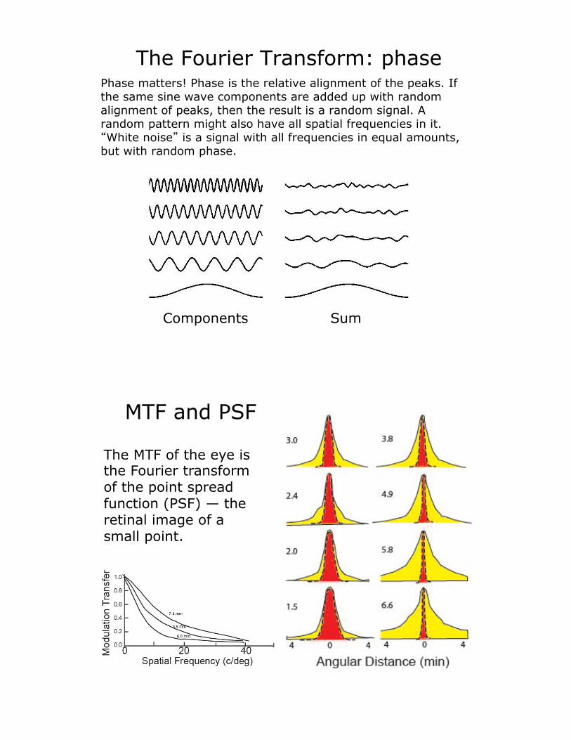
Effect of pupil size on modulation

transfer function (MTF), point spread function (PSF), and image appearance.

From Thibos & Applegate (2001) in Customized Corneal Ablation. MacRai, Krueger, Applegate, Eds

Contrast Sensitivity Function (CSF) The MTF describes the physical contrast of gratings on the retina. The CSF describes the ability of the visual system to detect gratings. The MTF limits this ability, but there are also neural factors involved. The CSF plots CS vs. SF on log-log axes, where CS = 1 / contrast threshold. Photopic CS is best for middle SFs (e.g. about 4 c/deg). We get worse (lower sensitivity) for SFs lower or higher than this.

Peak contrast sensitivity

High SF cut-off

Low SF roll-off

CSF and Acuity Grating resolution acuity depends on contrast

Con

tras

t S

ensi

tivi

ty

Spatial Frequency (c/deg)

High-Contrast acuity!

Low-Contrast acuity!

100%

10%

Common ways to Measure CSF

1. Use gratings presented on monitors.

2. Use printed grating patches (e.g., Vistech, CSV 1000).

3. Use low contrast letter charts (constant contrast, but letters vary in size).

4. Pelli-Robson chart (constant letter size, but letters vary in contrast).

The �VisTech� chart is a Contrast Sensitivity Test Using Grating Patches of varying spatial frequency and contrast

SF!

Contrast sensitivity!(This is just an example, not the actual chart)

Eye Charts like the Bailey-Lovie with high and low contrast letters provide two points on the CSF function:

high and low contrast acuity values.

High-contrast! Low-contrast!

Dec

reas

e in

siz

e!

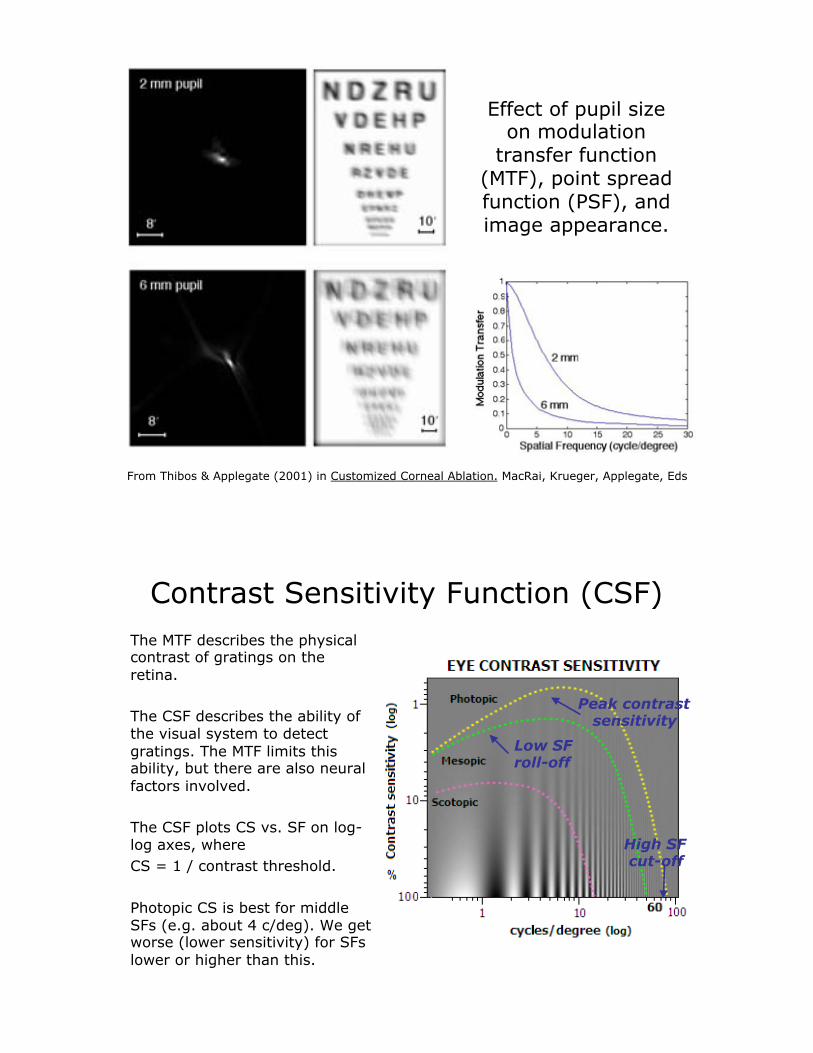
Pelli-Robson Chart

Used for measuring contrast sensitivity with letters of fixed size (0.5 deg at 3 meter viewing distance). The dominant spatial frequency of the letters is about 5 cycles per degree, near the peak of the normal contrast sensitivity function. Uses Sloan letters.

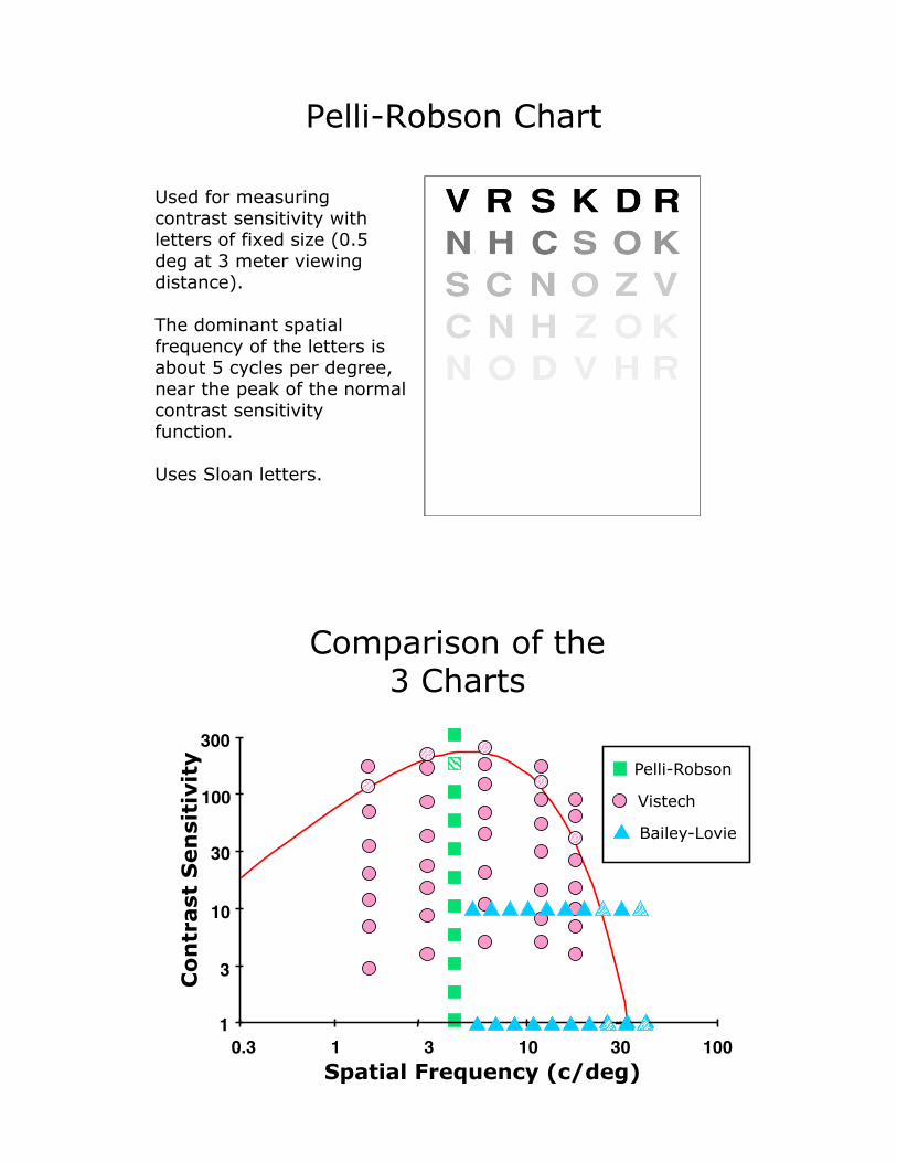
Comparison of the 3 Charts

.!1!

3!

10!

30!

100!

300!

0.3! 1! 3! 10! 30! 100!

Pelli-Robson!Vistech

Bailey-Lovie

Spatial Frequency (c/deg)!

Con

tras

t S

ensi

tivi

ty

Factors Affecting CSF

Luminance - best at high luminance Eccentricity - best in central vision Optical blur - best with perfect optics Age - best for young adults Temporal modulation - flicker helps us with low SF, hurts us with high SF

Luminance and CSF

1) Peak CS improves and shifts to higher SFs as luminance increases. 2) the high-SF cut-off (acuity) improves with luminance. 3) CS at Low SF does not change with luminance except when switching from rods to cones. This part of the data follows Weber�s law.

Contrast sensitivity in the periphery

The CSF changes if targets are presented in the periphery, but it matters how you do the test. If grating patches are scaled up with eccentricity, the CSF keeps the same shape.

No Scaling: Grating Patch at fixation is the same size as the one in the lower visual field

Scaling: Grating patch is made larger for increasing eccentricity.

How CSF changes with Eccentricity If the patch is kept the same size in the periphery, peak contrast sensitivity drops. If the size of the grating patch is increased in proportion to the eccentricity, the peak contrast sensitivity does not drop. Instead the function shifts toward lower SF and keeps almost the same shape.

No Scaling Scaling

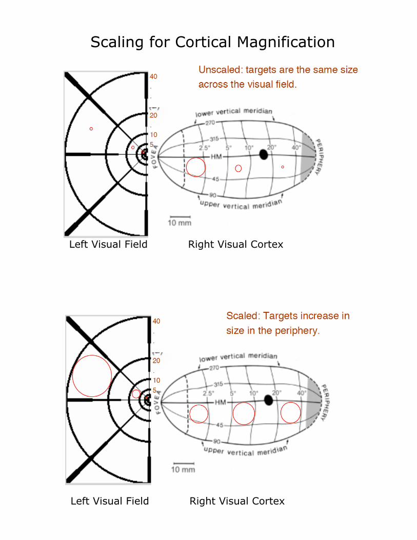
Scaling for Cortical Magnification

Left Visual Field Right Visual Cortex

Left Visual Field Right Visual Cortex

For targets scaled appropriately in size, CS is approximately constant across eccentricity when expressed in cortical units (cycles/mm of cortex).

Here the same data are replotted in terms of spatial frequency in the visual cortex (cycles / mm). They all line up!

Scaling for �Cortical Magnification�

Optical Blur Attenuates

CSF Blur decreases CS, especially at high SFs, because of the change in the MTF.

increase in blur!

MTF vs. CSF At high Spatial Frequencies, the MTF and foveal CSF are similar, indicating that the primary limitation on CS for high SFs is optical in the fovea. Optics does not explain the loss of acuity and high SF sensitivity in the periphery, because the optics of the eye are still pretty good there. The loss is due to the way images are sampled by cones, ganglion cells, and cortex. The limitations are neural, not optical.

Effect of Blur: Fovea vs. Periphery

Blur has less effect on acuity in the periphery than in the fovea. Blur has little effect on high SFs in the periphery because the high-SF cut off is not limited by optics.

Sp

atia

l fre

qu

ency

cu

toff

(

c/d

eg)

Age and CSF CS is initially very low in infants. Newborn acuity is around 6 c/deg, measured with Visual Evoked Potentials (VEP) . In adults, CS at high SF declines gradually with age.

Clinical Measurement of CSF

TV-based grating generators (e.g., Nicolet). CS charts (e.g. Vistech) using gratings. CS charts using letters. FPL (forced choice preferential looking) in infants.

Monocular vs. Binocular Viewing For people with normal vision in both eyes, contrast sensitivity is usually higher for binocular than for monocular viewing. Sensitivity is better with two eyes than with only one eye. Linear summation: 1+1=2 Probability summation: √2 = 1.41 Usually, increase in sensitivity due to binocular summation is between 1 to 1.41x. Subjects without functioning binocularity (like strabismics) will show little or no summation.

Replotted from Ross, Clarke & Bron (1985)

89

100

2

3

4

Con

tras

t Sen

siti

vity

3 4 5 61

2 3 4 5 610

2 3

Spatial Frequency (c/deg)

binocular monocular

Factors Accounting for the Shape of CSF

High SF attenuation: optical limitations in fovea Neural limitations in periphery

Low SF roll off: neural limitations in fovea and periphery

Spatial Frequency (c/deg)

Con

tras

t S

ensi

tivi

ty

Neurons are tuned for spatial frequency

7 c/deg!7 c/deg!

Adaptation to a single SF decreases CS at that and nearby SFs, suggesting that neurons tuned to limited SF bands underlie the normal CSF. Staring at a grating for a few minutes makes us less sensitive to gratings of similar spatial frequency. The spread of the adaptation effect suggests how wide the �channels� are in our visual system. The plot on the right shows the change.

Multi channel theory of CSF

The CSF is assumed to represent the combination of many SF-tuned neurons. Just the way color vision comes from three cone curves that overlap, but here we have many more overlapping curves.

SF Tuning Neurophysiology studies support the idea of many tuned Spatial Frequency �Channels.� Neurons in the visual system exhibit a range of SF tuning. SF tuning becomes narrower from the retina to the visual cortex.

Low-SF Roll-Off: Temporal Modulation

CS at low SFs improves with temporal modulation. The cells tuned for low frequencies are more sensitive to flickering gratings than steady ones.

Perceived Contrast Above threshold, perceived contrast increases faster for low and high SFs than middle SFs. Consequently, different SFs with physically equal supra-threshold contrast appear about the same. In this figure, each point represents a grating of some spatial frequency and contrast. Points connected by lines all appear to have the same contrast as the points in the middle at 5 cpd.