Using Random Forests to Describe Equity in Higher

Butler Journal of Undergraduate Research Butler Journal of Undergraduate Research

Volume 4

2018

Using Random Forests to Describe Equity in Higher Education: A Using Random Forests to Describe Equity in Higher Education: A

Critical Quantitative Analysis of Utah’s Postsecondary Pipelines Critical Quantitative Analysis of Utah’s Postsecondary Pipelines

Tyler McDaniel University of Utah, [email protected]

Follow this and additional works at: https://digitalcommons.butler.edu/bjur

Part of the Applied Mathematics Commons, Applied Statistics Commons, Educational Sociology

Commons, Higher Education Commons, Mathematics Commons, Multivariate Analysis Commons, and

the Statistical Methodology Commons

Recommended Citation Recommended Citation McDaniel, Tyler (2018) "Using Random Forests to Describe Equity in Higher Education: A Critical Quantitative Analysis of Utah’s Postsecondary Pipelines," Butler Journal of Undergraduate Research: Vol. 4 , Article 10. Retrieved from: https://digitalcommons.butler.edu/bjur/vol4/iss1/10

This Article is brought to you for free and open access by the Undergraduate Scholarship at Digital Commons @ Butler University. It has been accepted for inclusion in Butler Journal of Undergraduate Research by an authorized editor of Digital Commons @ Butler University. For more information, please contact [email protected].

https://digitalcommons.butler.edu/bjur

https://digitalcommons.butler.edu/bjur/vol4

https://digitalcommons.butler.edu/bjur?utm_source=digitalcommons.butler.edu%2Fbjur%2Fvol4%2Fiss1%2F10&utm_medium=PDF&utm_campaign=PDFCoverPages

http://network.bepress.com/hgg/discipline/115?utm_source=digitalcommons.butler.edu%2Fbjur%2Fvol4%2Fiss1%2F10&utm_medium=PDF&utm_campaign=PDFCoverPages








https://digitalcommons.butler.edu/bjur/vol4/iss1/10?utm_source=digitalcommons.butler.edu%2Fbjur%2Fvol4%2Fiss1%2F10&utm_medium=PDF&utm_campaign=PDFCoverPages

mailto:[email protected]

Using Random Forests to Describe Equity in Higher Education: A Critical Using Random Forests to Describe Equity in Higher Education: A Critical Quantitative Analysis of Utah’s Postsecondary Pipelines Quantitative Analysis of Utah’s Postsecondary Pipelines

Cover Page Footnote Cover Page Footnote Thanks to Erin Castro, for encouraging me to write clearly, think critically, and question power. Thanks to Braxton Osting, for advice of the highest caliber on algorithms, data, and the research process.

This article is available in Butler Journal of Undergraduate Research: https://digitalcommons.butler.edu/bjur/vol4/iss1/10

https://digitalcommons.butler.edu/bjur/vol4/iss1/10

https://digitalcommons.butler.edu/bjur/vol4/iss1/10

BUTLER JOURNAL OF UNDERGRADUATE RESEARCH, VOLUME 4

141

USING RANDOM FORESTS TO DESCRIBE EQUITY IN HIGHER EDUCATION: A CRITICAL QUANTITATIVE ANALYSIS OF UTAH’S POSTSECONDARY PIPELINES

TYLER MCDANIEL, UNIVERSITY OF UTAH MENTOR: ERIN CASTRO

Introduction

The goal of this work is to make a methodological contribution to the study of higher education. The Random Forest (RF) algorithm has proven useful in many fields due to its efficiency and accuracy in making predictions with large datasets (Breiman, 2002). Within the field of education, researchers are increasingly interested in the applications of large-scale, complex information systems (Daniel, 2015). As higher education data become more readily available, machine learning techniques such as RF have the potential to improve our understanding of student enrollment and success. For these reasons, RF is tested against more traditional models, using a state-wide longitudinal dataset. In order to contribute to the existing knowledge-base of higher education research in the United States in general and in Utah in particular, the methodological contributions of this work are grounded within a substantive context. This means that statistical techniques are discussed within the framework of critical quantitative scholarship, with the explicit motive of improving race, class, and gender equity in pathways to higher education. The results and implications of this work should be widely accessible for audiences with statistical, educational, or sociological interests.

Access to postsecondary education is an area of great import, due to the abundance of individual and societal benefits that accompany higher education. In addition to increased civic engagement and health, higher education spurs productivity and opens access to economic mobility (Perna and Swail, 2001). In 2014, those with Bachelor’s degrees earned 66% more than those with High School diplomas. For each subsequent education level, median incomes increased significantly (Kena et al., 2016). This is particularly meaningful in the context of social mobility because students from low and high income families who attend the same university have similar economic outcomes (Turner and Treasury, 2017). As a result, those who study education are becoming increasingly interested in access to postsecondary institutions.


142

While a college education is increasingly important in the global marketplace, state policies and practices are often ineffective at– and in fact discriminatory in – funneling well-qualified students into higher education (Kirst and Venezia, 2004). In order to improve the design of higher education access, it is crucial to dissect and critique the existing process. The following section will outline the racial, economic, and gender nuances of Utah’s higher education pipeline, in addition to reviewing national trends and common metrics for student success. The Introduction continues by situating the discussion within the critical quantitative framework, pointing out research gaps, and finally addressing the expected research contribution.

Race, Class, and Gender Context

Two relentless threats to equity in the U.S. education system are structural racism and class discrimination. The re-segregation of Black and Latinx public school students, combined with the lack of resources in high-poverty, high-racial minority school districts, has contributed to unyielding achievement gaps (Wald and Losen, 2003). Racial segregation is tied to the black-white achievement gap for a variety of reasons, most notably the disparity in poverty rates between black students’ and white students’ schools (Reardon, 2016). Nationally, Black students reside in classrooms where 64% of their classmates are low-income (Frankenberg and Orfield, 2012). Race and class inequities such as unequal access; underrepresentation in Science, Technology, Engineering and Mathematics (STEM) fields (which tend to be the most lucrative); dissimilar retention efforts; and disparate degree attainment continue to plague the mission of higher education (Bensimon and Bishop, 2012). Race gaps in educational opportunity are detrimental not only to students, but to society at large: inferior higher education and STEM pipelines for underrepresented minority (URM) students inevitably hurt U.S. competitiveness in a global market. This problem has been exacerbated by the growing populations of Non-White U.S. citizens (Hurtado, 2007; Chambers, 2009), for despite significant increases in the population of URM citizens, racial diversity at selective, public universities has declined (Garces and Cogburn, 2015). While advances in representation have been made, racial disparities continue to stymie equity in higher education.

Economic barriers to postsecondary education also diminish the integrity of education pipelines. Students whose parents are in the top 1% of the income distribution are roughly 77 times more likely than students whose parents are in the bottom quintile of the income distribution to attend an Ivy League institution


143

(Chetty et al., 2017). Students from low income families are underrepresented in every section of the education pipeline, and income disparities increase with each subsequent education level after high school (Jacobson and Mokher, 2009). Even controlling for student ability and familial background, neighborhood effects further contribute to students’ educational attainment (Garner and Raudenbush, 1991). Lack of financial information often contributes to depressed college enrollment for well-qualified low-income students (Kelchen & Goldrick-Rab, 2015). These gaps are striking in the college application process: Hoxby and Avery (2012) estimate that while high-achieving, high-income students outnumber high-achieving low-income students 2:1 in the general population, the high-income high achievers outnumber their low-income counterparts 15:1 in college applications to selective institutions. In addition to the financial barriers, students from low income families and communities often experience education pipelines and information networks not structured to maximize their academic potential.

Gender barriers in postsecondary education are nuanced: women fare well in terms of access to higher education, but often do not achieve similar outcomes. Nationally, women obtain degrees at higher rates than men. In 2015, half of women aged 25-29and 41% of men aged 25-29 had completed an Associate’s degree or higher, while 39% of women and 32% of men had completed a Bachelor’s degree or higher (Kena et al., 2016). However, higher degrees do not translate into similar levels of success across genders. This problem is exaggerated in Utah, where female graduates are dramatically undervalued in the workplace: When compared to similarly qualified individuals, women earn 97% of what men earn nationally, and only 86% of what men earn in Utah. Interestingly, inequality due to different endowments - the gender discrepancy in wages due to measurable education and career differences -is increasing (Miller, 2016). Within the heavily Mormon religious environment of Utah, higher education is deemed by some scholars as a form of embedded resistance for Latter Day Saints (LDS) women to negotiate the patriarchal hegemony (Mihelich and Storrs, 2003). Nevertheless, while women are attaining higher education at historic rates, Utah’s pipelines are fraught with inequities that detract from higher education’s mission of equal opportunity.

Finally, the influence of tools for measuring academic achievement cannot be over- stated. Although many admissions offices weight the two similarly, High School GPA typically predicts first year college GPA more accurately than standardized test scores (Sawyer, 2013). In addition to being a better predictor of initial student success, High School GPA has been shown to contain less bias against URM students than standardized test scores. In fact, when race and class


144

are ignored in post-secondary GPA predictive models, their effects are often absorbed into the standardized test component, calling into question the validity of such universal standards (Geiser and Santelices, 2007). Critics of standardized tests claim that test scores reflect Socio-Economic Status (SES) rather than ability, but there does seem to be a strong association between test scores and academic potential. In fact, test scores may predict success at more selective institutions with greater accuracy than High School GPA (Sawyer, 2013; Noble and Sawyer, 2004). When accounting for SES, test scores still are able to explain approximately 1

5 of

the variation in postsecondary grades (Sackett et al., 2009). Goals of this work include interrogating the utility and effectiveness of High School GPA, ACT scores, and AP scores in predicting postsecondary GPA. Additionally, this work seeks to critique the process via which demographic inequities may be reified by each assessment tool.

Critical Quantitative Framework

This work seeks to contribute to the field of critical quantitative inquiry in higher education. A critical perspective advances higher education research by countering false narratives, challenging previous work, and presenting alternative lenses (or methods). Originating from scholars of the Frankfurt School, critical theory focuses on identifying latent power structures and oppressions, and often manifests itself in efforts to change existing hierarchies. The work of critical theorists includes changing the methods used to interpret society as well as changing society itself (Kincheloe, McLaren, and Steinberg, 2012).This section defines the quantitative critical research model and points to the relevance of critical work for this manuscript.

Critical education theory has previously been associated with qualitative studies, which typically focus on presenting alternative social narratives in order to center the experience of marginalized individuals (Stage, 2007). The most important stage of the critical research process is widely considered the interpretation of results; critical scholars often reject notions of objectivity in research (Kincheloe and McLaren, 2002). Many qualitative critical theorists view quantitative work as reductive in nature (Stage, 2007). However, these critics may underestimate the importance of interpretation around statistical results. Statisticians often caution that their methods are not representations of objective reality, but rather a lens through which one can view data. Leo Brieman and Adele Cutler, the authors of the RF algorithm, the primary tool of analysis used in this


145

project, offer the following warning for consumers looking for objectivity in RF results:

RF is an example of a tool that is useful in doing analyses of scientific data. But the cleverest algorithms are no substitute for human intelligence and knowledge of the data in the problem. Take the output of random forests not as absolute truth, but as smart computer generated guesses that may be helpful in leading to a deeper understanding of the problem.

By providing novel insights through careful analysis rather than seeking objective measures of truth, critical quantitative theorists can add value to current education research. Critical approaches advance the field of education studies by measuring inequities and challenging oppressive narratives which rely on false objectivities. Thus, the quantitative critical theorist will (1) investigate equity of the educational world using data and (2) interrogate the usage of current empirical models in educational studies, in an effort to better represent marginalized groups (Stage, 2007). Advances in statistical algorithms (such as RF) are becoming useful for the quantitative critical scholar. The goals of the quantitative critical theorist, namely documenting inequities and challenging methods for representing those inequities, are increasingly viable due to surges in information and advances in statistical methodology.

Research Gaps

Previous researchers have used techniques such as Hierarchical Generalized Lin- ear Modeling or Multi-level Modeling (Hurtado, 2007; Raudenbush and Bryk, 2002; You and Nguyen, 2012), Structural Equation Modeling (Zajacova, Lynch, and Es- penshade, 2005), Network Analysis (Gerber and Schaefer, 2004), and Data Mining (Slater et al., 2017) to measure educational access and success. A small number of studies have used RF to predict students outcomes in Spanish, Brazilian, British, and Portuguese education systems (Blanch and Aluja, 2013; Cortez and Silva, 2008; Golino and Gomes, 2014; Hardman, Paucar-Caceres, and Fielding, 2013; Golino, Gomes, and Andrade, 2014). However, there is a lack of research examining the U.S. postsecondary system with machine learning techniques such as RF. Top journals such as Sociology of Education and The Journal of Educational and Behavioral Statistics have yet to publish studies using RF to describe inequality in higher education.


146

Location is an important factor in the progression to higher education (Turley, 2009). Topics such as racial, gender, and economic inequality in postsecondary education have not been thoroughly investigated for their influence in this process as well, and there is little research on the confluence of such factors in the state of Utah, where cultural processes such as the LDS mission disrupt traditional high school- to-college pipelines. Additionally, there is little quantitative work around higher education and gender in LDS environments, although the existing qualitative work suggests that higher education is a form of resistance for some Mormon women (Mihelich and Storrs, 2003). Simply put, Utah’s unique religious and gender context contributes to college-going in multifarious ways, raising important questions of demographic access and equity. The aforementioned traits also make Utah an interesting environment to test novel methods with complex data.

Lastly, the relevance of machine learning in the canon of critical quantitative studies in higher education remains unexplored. The RF framework aligns well with the critical quantitative model of inquiry, which seeks to interrogate both substantive and methodological assumptions. The RF model subverts notions of linearity in effects, allowing for new interpretations of demographic relationships. Both critical scholarship and RF research depend heavily on the interpretation of results. This work challenges assertions that quantitative work is reductive in nature, instead pointing toward similarities in quantitative and critical work, and exemplifying critical interpretations of RF analyses. While there is a growing body of critical quantitative higher education research, and RF is an established method in machine learning, the author is unaware of any previous work that synthesizes these two approaches.

Research Contribution

The goal of this work is to explore the RF algorithm as a method for making predictions in higher education. In this work, methods are tested within the context of race, class, and gender inequalities in higher education. Substantively, this work will further current knowledge on access to postsecondary education systems, with a focus on demographic inequities in the state of Utah. Methodologically, this work compares three quantitative models according to their efficacy in predicting student success. Results are interpreted through a quantitative critical lens. This work adds to a growing body of quantitative research on higher education access. As a non-linear, decision-tree-based, ensemble predictor, the RF model is structurally dissimilar from common prediction models, and offers some unique advantages.


147

Instead of using distance on an n-dimensional plane to maximize predictive efficacy, RF agglomerates large amounts of split-points. In each tree, a random subset of variables are used to make decisions, allowing the RF algorithm to capture some of the nuances of variable relationships. RF models have proven to be optimal predictors in a wide range of fields such as finance, biology, and chemistry. Given the accuracy, precision, simplicity and benefits of the RF model (Hastie, Tibshirani, and Friedman, 2001), the lack of studies using RF as a tool to predict student success in the U.S. higher education system is surprising.

Following Frances Stage’s model of critical quantitative inquiry, the goals of this work are to interrogate both the equity of Utah’s education pathways and the methods which are generally used to study higher education pathways. The present research attempts to answer the following questions:

(1) What inequities in access to higher education for Utah high school students are shown by Random Forest, logistic, and linear models?

(2) Can Random Forest predict student access success in higher education more accurately than logistic or linear estimators?

(3) How can the Random Forest algorithm advance quantitative critical higher education scholarship?

This paper is structured in the following manner: data organization, cleaning, and imputations are covered in Section 2. RF, linear, and logistic models are described in section 3. Research questions (1) and (2), which focus on substantial and methodological conclusions, respectively, are covered in Section 4. This work finds that the RF algorithm outperformed the logistic model, performed similarly to linear models, and in some cases offered a more complete understanding of student variables than other models. Finally, Section 5 answers research question (3), focusing on the broader importance of quantitative education studies. RF is considered useful in quantitative critical higher education research because it provides novel interpretations of data, allows for challenges to previous models, and can be used to advance equity.

Data

Source, Structure

Data were obtained from the Utah System of Higher Education, and include information on 43,947 students from the 2008 cohort of Utah high school graduates. Every student who was recorded in a Utah high school as part of this cohort was


148

included, regardless of actual high school graduation status. Demographic information such as school district, school, gender, race, low income status, mobility, English learner status, migrant status, and special education status was included. Gender was denoted as binary (male/female). Race was divided into ten categories: Caucasian, White not of Hispanic Origin, Black, Asian, Hispanic or Latino, American Indian, Pacific Islander, Multiple Race, and missing. This work is limited by the fact that gender and race categories available are not exhaustive, and do not represent every identity of interest. Low income status was indicated for students who qualify for the National School Lunch Program (free or reduced price lunch) or who have been identified as economically disadvantaged on another measure during their final year of high school enrollment. Mobile status was indicated if a student did not attend the same high school for the entirety of that student’s final year of enrollment. Migrant status was indicated if the student has been identified as the child of migratory agricultural workers. Special Education status was indicated if students participated in special education during their final year of high school. The English Language Learner variable indicates whether a student participated in a Limited English Program during their final year of high school. Student achievement information such as Advanced Placement (AP) test scores, ACT test scores, High School GPA, and High School college enrollment was included. ACT test scores are disaggregated by Reading, English, Mathematics, Science and Composite results. Postsecondary information such as Pell Grant eligibility, Pell Grant reception, postsecondary GPA, semester start date, and Classification of Instructional Program (CIP) were also provided for each semester a student was enrolled in an institution of higher education.

Data were received from the Utah Data Alliance, through the National Student Clearinghouse, in four sets, with rows corresponding to student ID, semester, degree, and standardized test result, respectively. In order to test the variety of relationships between student variables provided, data were merged such that each row pertained to one of the 41,303 students. This merged dataset included 186 variables, many of which were ultimately not pertinent to the research question. In figure 1, one can see a visual representation of the data used to measure college pathways. The complexity of using pathways to describe college access is readily ascertained, as many students attend college at different times, take breaks, and graduate on different schedules. For this reason, students may be counted in multiple stages of the pathways. Even so, there is a basic structure to the institutions and opportunities that accessible to students.


149

Variables Created

Many variables were created in order to summarize the students’ higher education experiences. A URM indicator was created based on whether students’ race was one of the following categories: Caucasian, White not of Hispanic origin, or Asian, based on previous research on URM students (Hurtado et al., 2009). Semester start dates were sorted from oldest to newest, and Cumulative GPA was created using the most recent GPA result from a student’s postsecondary career. Earliest Enrollment was created using the year that each student first enrolled in postsecondary classes. College Semesters in High School was created using the number of postsecondary-level courses that the student took prior to High School graduation. Two college enrollment variables were generated based on the 28,878 unique Person ID values which had college enrollment data: College in High School, indicating whether students had taken postsecondary courses prior to Summer 2008, and College Attainment, indicating whether students had attained college after Spring 2008.

Figure 1. A summary of pathways to higher education for students in the state of Utah; the number of students enrolled in various institutions is indicated (students may transfer, and thus be counted in multiple institutions).

Classification of Instructional Programs (CIP) codes were used to identify STEM majors, based on the U.S. Immigrations and Customs Enforcement STEM-Designated Degree Program List 2012. STEM students were identified based on


150

the National Center for Education Statistics definition of STEM students, which includes any student who has participated in at least one semester of a STEM major (Chen and Weko, 2009). STEM status was indicated if a student had participated in a STEM major. The creation of STEM status and other variables allowed the researcher to summarize meaningful student information so that it could be incorporated in predictive models.

Missing Data

Missing data is a common problem in education studies. Many items in the present dataset were missing, such as district, school, gender, race, low income status, mobile status, High School GPA, ACT scores, and Pell Grant eligibility. Observations which were missing information for district, school, gender, race, migrant status, mobile status, English learner status, and Special Education status (n = 2644) were removed using listwise deletion. This technique refers to the removal of entire rows of data with missing values. Although listwise deletion is typically not recommended in the case of missing data, there was little advantage in keeping cases which had no demographic information. Additionally, cases in which the individual had no High School GPA (n = 56) were removed using listwise deletion. Because n is small, in this case 0.15% of the data, such removal is not problematic.

Table 1. Students without ACT scores are academically different than those with ACT scores.

Many students (44.3% of the 28,878 students who had a record of higher education) were missing ACT scores, likely because they did not take the test. Test scores can be an important predictor of academic success, and in order to utilize this predictor without removing large amounts of data, estimation of missing data was necessary. There is reason to believe that ACT test scores are not missing at random (MAR): students who do not have ACT scores exhibit notable academic differences from their peers. Thus missing data are classified as nonignorable, as


151

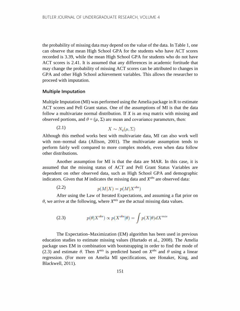
the probability of missing data may depend on the value of the data. In Table 1, one can observe that mean High School GPA for the students who have ACT scores recorded is 3.39, while the mean High School GPA for students who do not have ACT scores is 2.41. It is assumed that any differences in academic fortitude that may change the probability of missing ACT scores can be attributed to changes in GPA and other High School achievement variables. This allows the researcher to proceed with imputation.

Multiple Imputation

Multiple Imputation (MI) was performed using the Amelia package in R to estimate ACT scores and Pell Grant status. One of the assumptions of MI is that the data follow a multivariate normal distribution. If X is an nxq matrix with missing and observed portions, and θ = (µ, Σ) are mean and covariance parameters, then:

(2.1)

Although this method works best with multivariate data, MI can also work well with non–normal data (Allison, 2001). The multivariate assumption tends to perform fairly well compared to more complex models, even when data follow other distributions.

Another assumption for MI is that the data are MAR. In this case, it is assumed that the missing status of ACT and Pell Grant Status Variables are dependent on other observed data, such as High School GPA and demographic indicators. Given that M indicates the missing data and Xobs are observed data:

(2.2)

After using the Law of Iterated Expectations, and assuming a flat prior on θ, we arrive at the following, where Xmis are the actual missing data values.

(2.3)

The Expectation–Maximization (EM) algorithm has been used in previous education studies to estimate missing values (Hurtado et al., 2008). The Amelia package uses EM in combination with bootstrapping in order to find the mode of (2.3) and estimate θ. Then Xmis is predicted based on Xobs and θ using a linear regression. (For more on Amelia MI specifications, see Honaker, King, and Blackwell, 2011).


152

The Amelia algorithm was specified such that the range of ACT scores is restricted to 0–36, and the range of Pell Grant statuses is restricted to 0–1. The algorithm achieves this by discarding any estimated values that appear outside of these ranges. Because the estimated parameters of ACT scores and Pell Grant eligibility are discrete, the estimated values were rounded to the nearest integer. The imputations were performed five times. MI estimations generally become more accurate after each iteration is performed (Allison, 2001), so the fifth imputation was used in order to replace missing data.

Methods

Random Forest Background

A myriad of measures related to postsecondary access and success are common in education literature, and still many institutions are unaware of the variables that best predict student progress. While many methods have been used to represent student progression in higher education, a growing body of research seeks to understand this process through large datasets of interrelated variables. RF algorithms are increasingly popular in the prediction of student achievement due to their accuracy and fluency in analyzing large amounts of information (Blanch and Aluja, 2013; Cortez and Silva, 2008; Golino and Gomes, 2014; Hardman, Paucar-Caceres, and Fielding, 2013). Hardman and Paucar-Caceres used RF in order to predict a student’s progression in higher education, evaluating indicators for success in a virtual learning environment. RF was promoted for its utility in higher education research in this study due to its efficacy with large datasets (2013). Golino, Gomes, and Andrade (2014) state that RF is of particular interest to the field of educational research due to its ability to identify predictive variables and address the non-linearity in predictive power of individual variables, referring to the partial plot feature of RF. In Golino, Gomes and Andrade’s (2014) study predicting the academic success of high school students, RF is commended due to its fluency and lack of assumptions (such as normality, collinearity, homoscedasticity, independence between variables). Additionally, Hardman, Paucar-Caceres, Urquhart, and Fielding use RF to make two contributions to the study of information systems in higher education: (1) defining key variables for university student progression in a VLE and (2) introducing RF as an optimal method for analyzing such information (2010). Variable importance and partial plots are used in order to distinguish critical variables for advancement in the VLE, such as usage time and staff page visits. Of the aforementioned works using RF, all evaluate educational systems outside the United States, and none use RF to critically


153

interrogate demographic influence. Therefore, the RF model remains relatively unexplored as a tool for describing equity in higher education in the United States.

RF is a powerful prediction tool in fields outside of education. In terms of accuracy, Leo Breiman and Adele Cutler state that the RF algorithm is unexcelled by other modern algorithms (2001). The algorithm does remarkably well in prediction, even without much tuning (Hastie, Tibshirani, and Friedman, 2001). In addition to accuracy, Classification and Regression Trees (CART) such as RF are optimal estimators due to their intuitiveness, fluency and ease of use (Golino and Gomes, 2014). Although RF algorithms were developed in statistics (Breiman et al., 1984) and machine learning (Quinlan, 1993), RF methods have been used effectively to make predictions in a wide range of fields, including systems biology (Geurts, Irrthum, and Wehenkel, 2009), molecular biology (Guerts, Irrthum, & Wehenkel, 2009), ADHD diagnosis (Skogli et al., 2013), medicinal chemistry (Naeem, Hylands, and Barlow, 2012), and finance (Khaidem, Saha, and Dey, 2016). In an influential study of cheminformatics, Svetnik et al. show that RF is among the most accurate predictors available, lauding its features of built-in performance assessment and relative importance measures (2003). A seminal work in gene selection used RF due to its ability to predict despite many variables being noisy (Díaz-Uriarte and De Andres, 2006). Many researchers have used RF algorithms in order to predict credit risk, a field in which misclassification can be costly (Brown and Mues, 2012; Iturriaga and Sanz, 2015; Wang et al., 2011). The use of Random Forest algorithms in diverse and complex fields illustrates the power and utility of the algorithm.


154

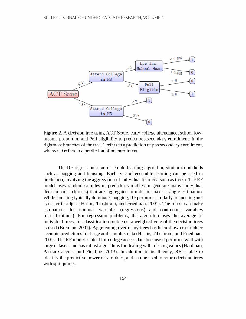
Figure 2. A decision tree using ACT Score, early college attendance, school low-income proportion and Pell eligibility to predict postsecondary enrollment. In the rightmost branches of the tree, 1 refers to a prediction of postsecondary enrollment, whereas 0 refers to a prediction of no enrollment.

The RF regression is an ensemble learning algorithm, similar to methods such as bagging and boosting. Each type of ensemble learning can be used in prediction, involving the aggregation of individual learners (such as trees). The RF model uses random samples of predictor variables to generate many individual decision trees (forests) that are aggregated in order to make a single estimation. While boosting typically dominates bagging, RF performs similarly to boosting and is easier to adjust (Hastie, Tibshirani, and Friedman, 2001). The forest can make estimations for nominal variables (regressions) and continuous variables (classifications). For regression problems, the algorithm uses the average of individual trees; for classification problems, a weighted vote of the decision trees is used (Breiman, 2001). Aggregating over many trees has been shown to produce accurate predictions for large and complex data (Hastie, Tibshirani, and Friedman, 2001). The RF model is ideal for college access data because it performs well with large datasets and has robust algorithms for dealing with missing values (Hardman, Paucar-Caceres, and Fielding, 2013). In addition to its fluency, RF is able to identify the predictive power of variables, and can be used to return decision trees with split points.


155

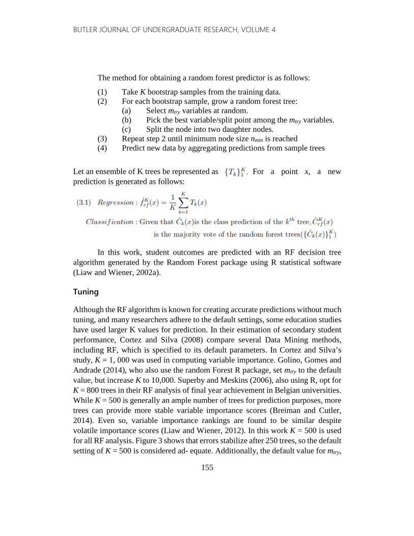
The method for obtaining a random forest predictor is as follows:

(1) Take K bootstrap samples from the training data. (2) For each bootstrap sample, grow a random forest tree:

(a) Select mtry variables at random. (b) Pick the best variable/split point among the mtry variables. (c) Split the node into two daughter nodes.

(3) Repeat step 2 until minimum node size nmin is reached (4) Predict new data by aggregating predictions from sample trees

Let an ensemble of K trees be represented as . For a point x, a new prediction is generated as follows:

In this work, student outcomes are predicted with an RF decision tree

algorithm generated by the Random Forest package using R statistical software (Liaw and Wiener, 2002a).

Tuning

Although the RF algorithm is known for creating accurate predictions without much tuning, and many researchers adhere to the default settings, some education studies have used larger K values for prediction. In their estimation of secondary student performance, Cortez and Silva (2008) compare several Data Mining methods, including RF, which is specified to its default parameters. In Cortez and Silva’s study, K = 1, 000 was used in computing variable importance. Golino, Gomes and Andrade (2014), who also use the random Forest R package, set mtry to the default value, but increase K to 10,000. Superby and Meskins (2006), also using R, opt for K = 800 trees in their RF analysis of final year achievement in Belgian universities. While K = 500 is generally an ample number of trees for prediction purposes, more trees can provide more stable variable importance scores (Breiman and Cutler, 2014). Even so, variable importance rankings are found to be similar despite volatile importance scores (Liaw and Wiener, 2012). In this work K = 500 is used for all RF analysis. Figure 3 shows that errors stabilize after 250 trees, so the default setting of K = 500 is considered adequate. Additionally, the default value for mtry,


156

𝑝𝑝3

= 223

= 7 is used for the number of variables to try at each split point. While tuning of K and mtry values was considered, ultimately the default settings were considered adequate for the purposes of this work.

RF Variable Importance, Partial Plots

The RF algorithm can be used evaluate variable importance, a measure of the influence of a particular variable on outcomes of prediction trees. Variable importance is a measure of the increase in Out of Bag (OOB) error, with a permutation of the variable of interest (Liaw and Wiener, 2002b). The OOB error refers to the error of the trees which do not include the variable of interest as a predictor. (Recall that because mtry is roughly 1

3 the total number of predictive

variables, roughly 23 of the trees generated will not include the variable of interest).

The partial plot provides a powerful visual representation of the marginal effect a predictor has on the response variable. It allows the researcher to isolate one real-valued variable x and view its partial dependence, . . Partial plots are obtained using the average values for all other variables, xiC in order to measure the change in prediction that occurs when the variable of interest, x, is manipulated (Liaw and Wiener, 2012). While the shape of the partial plots and relative scale of the vertical axis are important, the vertical axis values are not meaningful, as results represent change after integration over all other variables (Liaw, 2009). For regression, the change in prediction is measured with the following formula:

(3.2)

where x is the variable of interest, and xC is simply the complement of x, such that x∪xC = X, or every variable in the model (Hastie, Tibshirani, and Friedman, 2001).

Linear Models

Two linear models are used to estimate student success in higher education. The Ordinary Least Squares (OLS) regression method is a common tool in educational and sociological multivariate analysis (Dismuke and Lindrooth, 2006). OLS is a linear estimator that minimizes squared residuals in order to estimate new data. The OLS regression is denoted:


157

(3.3)

such that β are coefficients, Xj represent individual student variables, and ∈𝑖𝑖𝑖𝑖 are error terms.

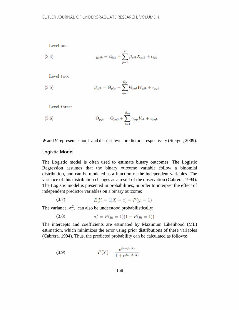
The OLS model does not control for groupings in data, such as districts or schools, which have been shown to significantly influence a child’s educational trajectory (Burtless, 2011). The Hierarchical Linear Model (HLM) adds new levels of analysis to the linear regression. In this model, coefficients estimated at one level become outcomes at the next level (Raudenbush and Bryk, 1986). The multi-level nature of this model allows one to nest students within schools, and schools within districts. This is helpful in separating the effects of individual characteristics and group characteristics. The nlme package in R was used to perform analysis, using Random Effects (RE) for district- and school-level characteristics and Fixed Effects (FE) for individual-level characteristics. The RE model allows for the estimation of the effects of group-level characteristics, such as racial and socioeconomic composition, and thus is quite popular in the social sciences for measuring higher-order effects. The FE model is based on the assumption that one true effect exists across studies, and thus do not estimate the sampling error variance. Therefore, FE models cannot suffer from heterogeneity bias, and are often used in econometrics to control for individual-level qualities (Bell and Jones, 2015; Snijders and Bosker, 1999). To account for high school-level differences in post-secondary retention and success, a random-intercept model is used where i are students, j are schools, and k are districts. The within-group error, ∈𝑖𝑖𝑖𝑖𝑖𝑖, between-school error 𝓇𝓇𝑝𝑝𝑖𝑖𝑖𝑖, and between-district error 𝓊𝓊𝑝𝑝𝑝𝑝𝑖𝑖, are assumed to be normal such that:


158

W and V represent school- and district-level predictors, respectively (Steiger, 2009).

Logistic Model

The Logistic model is often used to estimate binary outcomes. The Logistic Regression assumes that the binary outcome variable follow a binomial distribution, and can be modeled as a function of the independent variables. The variance of this distribution changes as a result of the observation (Cabrera, 1994). The Logistic model is presented in probabilities, in order to interpret the effect of independent predictor variables on a binary outcome:

(3.7)

The variance, 𝜎𝜎𝑖𝑖2, can also be understood probabilistically:

(3.8)

The intercepts and coefficients are estimated by Maximum Likelihood (ML) estimation, which minimizes the error using prior distributions of these variables (Cabrera, 1994). Thus, the predicted probability can be calculated as follows:

(3.9)


159

In this case, a logistic model is used to predict college attainment. Yi represents a student’s success (1) or failure (0) to enroll in postsecondary education after Spring 2008. The model is performed using the glm package in R.

Results

In order to assess the accuracy of predictive models, it is appropriate to split data into training and test sets (Breiman, 2001). For the purposes of this study, a random sample of 3,740 data points (10% of viable observations) were selected as test data, and the remainder of the data were used as the training set. After using the training data to specify each model, test set values were predicted. Comparisons between methods are based on the accuracy of predictions for the test data. The tables and figures in this section present the results of linear, logistic, and RF predictions.

It is difficult to directly compare the results of linear and RF regression models. In order to do so, a variety of measures were invoked to gauge the predictive qualities of each. Tables 2 and 4 display the results of OLS and HLM prediction of student success (GPA). The six number summaries (Tables 3 and 5) capture the accuracy of the linear and RF models, depicting measures of centrality and ranges for each model’s estimated values and error terms. Figure 3 represents the success of the RF model in predicting GPA (the average error as trees increase), as well as the importance of each variable to the predictive trees. Figure 4 expands our understanding of each variable’s predictive utility by showing the relationships between value and importance. Figure 5 adds visual context to the six number summaries, presenting a histogram and a density plot of the linear and RF error terms. In figure 6, predicted GPA is mapped onto actual GPA, displaying the variation in predictions for each model. The comparison of enrollment predictors was much more straightforward. Confusion matrices, displaying the number of correct and incorrect classifications, are used in figure 6 to compare the Logistic model and RF model.

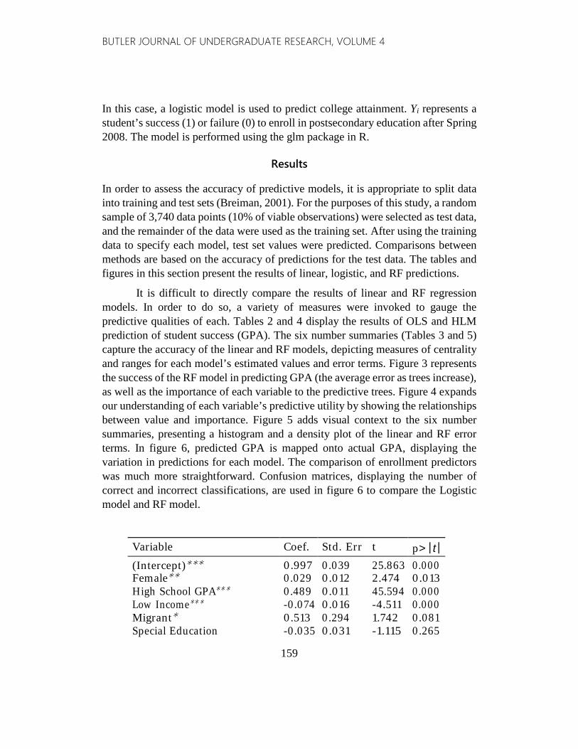
Variable Coef. Std. Err t p> |t| (Intercept)∗∗∗ 0.997 0.039 25.863 0.000 Female∗∗ 0.029 0.012 2.474 0.013 High School GPA∗∗∗ 0.489 0.011 45.594 0.000 Low Income∗∗∗ -0.074 0.016 -4.511 0.000 Migrant∗ 0.513 0.294 1.742 0.081 Special Education -0.035 0.031 -1.115 0.265


160

Mobile∗∗∗ 0.039 0.014 2.797 0.005 Limited English -0.011 0.057 -0.194 0.846 Attend College HS∗∗∗ 0.036 0.003 11.228 0.000 Pell Eligible 0.048 0.040 1.191 0.234 Pell Grant∗∗∗ 0.113 0.041 2.775 0.006 AP Scores > 3∗∗∗ 0.057 0.005 10.761 0.000 URM∗∗ -0.051 0.020 -2.588 0.010 ACT Read -0.004 0.004 -0.971 0.332 ACT Math∗∗ 0.010 0.004 2.373 0.018 ACT English 0.006 0.004 1.389 0.165 ACT Science -0.003 0.004 -0.653 0.514 ACT Composite 0.004 0.016 0.250 0.803 STEM∗∗∗ -0.078 0.015 -5.180 0.000 Low Income District

∗∗∗ -0.916 0.127 -7.211 0.000

Low Income School Mean -0.003 0.117 -0.022 0.983 URM District Mean ∗∗∗ 1.038 0.138 7.506 0.000 URM School Mean -0.012 0.121 -0.101 0.919

Table 2. Coefficients for OLS estimation of Postsecondary GPA *=significant at α = 0.1, **=significant at α = 0.05,***=significant at α = 0.01

Six Number Summaries: GPA Estimation Min 1st Quartile Median Mean 3rd Quartile Max

Actual Data 0.029 2.550 3.133 2.952 3.570 4.000 Random Forest 1.115 2.573 2.884 2.921 3.280 3.961 Linear Model 1.346 2.672 2.974 2.933 3.233 4.181

Hierarchical Linear Model

1.228 2.656 2.979 2.930 3.251 4.274

Table 3. The RF estimator outperforms OLS and HLM models in all prediction metrics except mean and median.

Variable Coef. Std. Err DF t p> |t| (Intercept)∗∗∗ 0.963 0.096 18106 10.055 0.000 Female 0.013 0.012 18106 1.146 0.251 High School GPA∗∗∗ 0.556 0.011 18106 48.717 0.000 Low Income∗∗∗ -0.069 0.016 18106 -4.274 0.000 Migrant∗ 0.560 0.290 18106 1.930 0.054 Special Education -0.025 0.031 18106 -0.806 0.420


161

Mobile 0.018 0.016 18106 1.160 0.246 Limited English -0.044 0.056 18106 -0.791 0.429 Attend College HS∗∗∗ 0.030 0.004 18106 8.669 0.000 Pell Eligible 0.018 0.040 18106 0.473 0.636 Pell Grant∗∗∗ 0.149 0.041 18106 3.638 0.000 AP Scores > 3∗∗∗ 0.054 0.005 18106 10.109 0.000 URM -0.031 0.019 18106 -1.591 0.112 ACT Read -0.003 0.004 18106 -0.758 0.448 ACT Math∗∗ 0.008 0.004 18106 1.971 0.049 ACT English 0.007 0.004 18106 1.578 0.115 ACT Science -0.002 0.004 18106 -0.473 0.637 ACT Composite 0.001 0.015 18106 0.038 0.970 STEM∗∗∗ -0.073 0.015 18106 -4.894 0.000 Low Income District Mean ∗ -0.697 0.398 52 -1.752 0.086 Low Income School Mean∗ -0.339 0.180 103 -1.877 0.063 URM District Mean 0.334 0.445 52 0.750 0.457 URM School Mean∗ 0.331 0.199 103 1.665 0.099

Table 4. Coefficients for HLM estimation of Postsecondary GPA *=significant at α = 0.1, **=significant at α = 0.05,***=significant at α = 0.01

Six Number Summaries: Error Terms (Predicted GPA–Actual GPA)

Min 1st Quartile Median Mean 3rd Quartile Max

Random Forest -2.029 -0.440 -0.107 -0.031 0.274 2.749 Linear Model -2.316 -0.445 -0.125 -0.019 0.308 2.833

Hierarchical Linear Model

-2.511 -0.451 -0.122 -0.022 0.312 2.912

Table 5. The RF estimator outperforms OLS and HLM models in all error metrics except mean.


162

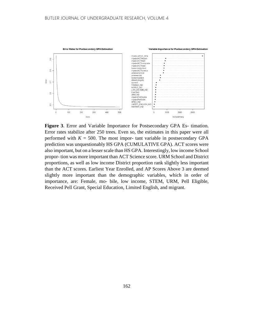
Figure 3. Error and Variable Importance for Postsecondary GPA Es- timation. Error rates stabilize after 250 trees. Even so, the estimates in this paper were all performed with K = 500. The most important variable in postsecondary GPA prediction was unquestionably HS GPA (CUMULATIVE GPA). ACT scores were also important, but on a lesser scale than HS GPA. Interestingly, low income School proportion was more important than ACT Science score. URM School and District proportions, as well as low income District proportion rank slightly less important than the ACT scores. Earliest Year Enrolled, and AP Scores Above 3 are deemed slightly more important than the demographic variables, which in order of importance, are: Female, mobile, low income, STEM, URM, Pell Eligible, Received Pell Grant, Special Education, Limited English, and migrant.


163

Figure 4. Partial plots of RF Postsecondary GPA Prediction, in order of variable importance (left to right, top to bottom). Predictions of postsecondary GPA surge when HS GPA increases, as well as ACT scores. Interestingly, GPA predictions decline after most ACT scores pass the 20-30 range. GPA predictions decline as low income School, URM School, and low income District percentages rise. URM District percentage follows a slightly diff t pattern, peaking between 30-40%. Lesser Earliest Year Enrolled values are associated with an increase in postsecondary GPA prediction. Additionally, predictions peak for 2 AP scores above 3. Female status, Pell Eligibility, and Pell Grant reception, are all associated with an increase in postsecondary GPA predictions, while mobile status, low income status, STEM fi status, and URM status are associated with declines in postsecondary GPA predictions.


164

Figure 5. Histogram and density plot of test set errors for linear models as well as RF model. Although the mean error for the RF model is slightly larger than the others, clearly the RF model is the more accurate estimator.

Figure 6. Visualization of Actual and Predicted Values, for Random Forest (left), Ordinary Least Squares (middle), and Hierarchical Linear Modeling (right). One may note the similarities between the estimations for both linear models. The RF model appears to more accurately estimate low performing college students, although it tends to underestimate high performers.


165

Logistic Model: Test Set Confusion Matrix Predicted Values 0 1 Class Error Actual 0 821 557 0.4042 Values 1 366 1996 0.1550

Random Forest Model: Test Set Confusion Matrix Predicted Values 0 1 Class Error Actual 0 921 457 0.3316 Values 1 388 1974 0.1643

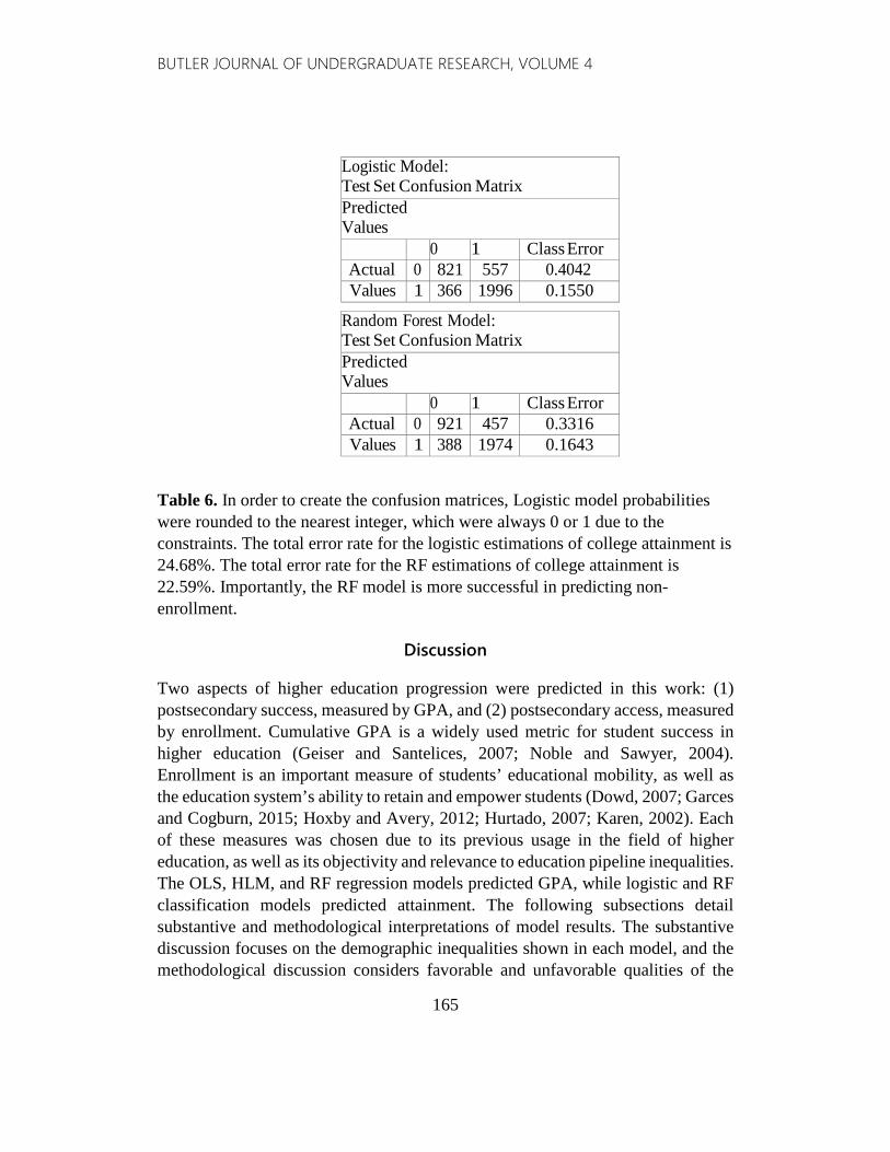
Table 6. In order to create the confusion matrices, Logistic model probabilities were rounded to the nearest integer, which were always 0 or 1 due to the constraints. The total error rate for the logistic estimations of college attainment is 24.68%. The total error rate for the RF estimations of college attainment is 22.59%. Importantly, the RF model is more successful in predicting non-enrollment.

Discussion

Two aspects of higher education progression were predicted in this work: (1) postsecondary success, measured by GPA, and (2) postsecondary access, measured by enrollment. Cumulative GPA is a widely used metric for student success in higher education (Geiser and Santelices, 2007; Noble and Sawyer, 2004). Enrollment is an important measure of students’ educational mobility, as well as the education system’s ability to retain and empower students (Dowd, 2007; Garces and Cogburn, 2015; Hoxby and Avery, 2012; Hurtado, 2007; Karen, 2002). Each of these measures was chosen due to its previous usage in the field of higher education, as well as its objectivity and relevance to education pipeline inequalities. The OLS, HLM, and RF regression models predicted GPA, while logistic and RF classification models predicted attainment. The following subsections detail substantive and methodological interpretations of model results. The substantive discussion focuses on the demographic inequalities shown in each model, and the methodological discussion considers favorable and unfavorable qualities of the


166

models. As noted in the introduction, interpretation is the crux of quantitative critical analysis, and is crucial in contextualizing the RF model.

Substantive Discussion

What inequities in access to higher education for Utah high school students are shown by Random Forest, logistic, and linear models?

According to both RF and linear models, High School GPA is the most important predictor of postsecondary GPA. In Tables 2 and 4, one can observe that every unit increase in High School GPA is associated with approximately a half-unit increase in postsecondary GPA. Figure 3 shows that ACT scores are the most important predictors following High School GPA, although the most predictive ACT Scores (English and Math) were less than one-third as important as High School GPA. Linear models indicate that ACT Math is the strongest predictor of postsecondary GPA, and is a significant positive predictor in both OLS and HLM models at the α = 0.05 level but not the α = 0.01 level. The effects of AP scores are highly significant (p < 0.001), although the GPA increase associated with each AP score above 3 is approximately one-tenth that of a one unit increase in High School GPA (0.054 units compared to 0.556 units, according to the HLM model). Similarly, OLS and HLM models indicate that High School college attendance is significant at the α = 0.01 level, but each course is associated with less than a 0.04 unit increase in GPA. In figure 4, one can observe that postsecondary GPA predictions continue to increase as High School GPA reaches its upper limit, while postsecondary GPA predictions decline as the ACT, AP, and High School college attendance variables approach their respective upper limits. This finding calls into question the use of ACT and AP scores as measures of potential success for high achieving students. When modeling postsecondary success, as measured by Cumulative GPA, AP scores, ACT scores, and High School college attendance are marginally predictive compared to High School GPA.

The importance plot in figure 3 suggests that gender is more important than all other demographic factors in modeling postsecondary GPA. According to partial plots, female gender is positively associated with predictions in postsecondary GPA. While the OLS model supports the notion that female gender is a positive predictor of academic success (significant at the α = 0.05 level), the HLM model suggests that gender is not a significant predictor. Additionally, previous studies suggests that this relationship does not hold across many areas of study such as STEM fields (Beede et al., 2011). The OLS model associates female status with less than a 0.03 unit increase in GPA. The goals of this work do not include


167

predicting STEM involvement or post-college outcomes, although it is clear that further exploration of the gender impact on college success could enhance this work. Female status appears to be a positive predictor of postsecondary success, yet results are mixed around the size and scope of this relationship.

Pell Grants were fairly important relative to other demographic traits; both OLS and HLM models list Pell Grant reception as a positive coefficient. Additionally, partial plots show that Pell Grant reception is a positive predictor of postsecondary

GPA in the RF algorithm. These relationships indicate that Pell Grants may have a compensatory effect for the consistent disadvantage that low income students face (low income status was associated with a 0.07 unit decline in GPA according to OLS and HLM models). Pell Eligibility was not significant in OLS or HLM models, while Pell Grant reception was significant at the α = 0.01 level in both models, corresponding to more than a 0.1 unit increase in GPA in each case. Pell Grants may be an incredibly effective tool in mitigating the structural burdens that plague economically disadvantaged students. However, in the RF estimation, Pell Eligibility was also a positive predictor of GPA, and slightly more important than Pell Grant reception. Reasons for this finding are unclear. Although Pell Grants appear to significantly increase the success of low income students, it may be useful to further study students who are eligible for Pell Grants but do not receive them.

Some of the most important variables under consideration were the proportions of URM and low income students housed within a school or district. The OLS model suggests that the proportion of URM students in a school district is positively associated with Postsecondary GPA, and the HLM model finds no relationship between these variables. The RF model shows that the effect of URM student proportion is not linear; the predicted success of students declines if they originate from a district with more than 30% URM students. Similarly, RF postsecondary GPA predictions decline as the proportion of URM students in a High School rises past 30%, although this relationship is insignificant in the OLS model and positively significant at the α = 0.1 level in the HLM model. According to OLS and HLM models, High School low income proportion was a negative predictor of postsecondary success (significant at α = 0.01 and α = 0.1, respectively). District low income proportion was significantly negative at the α = 0.1 level in the HLM model as well. Partial plots showed steadily declining postsecondary GPA predictions as High School and District low income proportions increased. RF and linear models suggested that higher proportions of


168

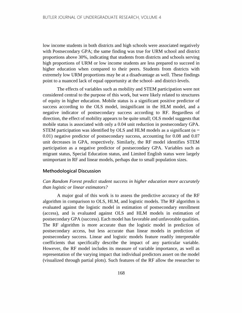
low income students in both districts and high schools were associated negatively with Postsecondary GPA; the same finding was true for URM school and district proportions above 30%, indicating that students from districts and schools serving high proportions of URM or low income students are less prepared to succeed in higher education when compared to their peers. Students from districts with extremely low URM proportions may be at a disadvantage as well. These findings point to a nuanced lack of equal opportunity at the school- and district-levels.

The effects of variables such as mobility and STEM participation were not considered central to the purpose of this work, but were likely related to structures of equity in higher education. Mobile status is a significant positive predictor of success according to the OLS model, insignificant in the HLM model, and a negative indicator of postsecondary success according to RF. Regardless of direction, the effect of mobility appears to be quite small; OLS model suggests that mobile status is associated with only a 0.04 unit reduction in postsecondary GPA. STEM participation was identified by OLS and HLM models as a significant (α = 0.01) negative predictor of postsecondary success, accounting for 0.08 and 0.07 unit decreases in GPA, respectively. Similarly, the RF model identifies STEM participation as a negative predictor of postsecondary GPA. Variables such as migrant status, Special Education status, and Limited English status were largely unimportant in RF and linear models, perhaps due to small population sizes.

Methodological Discussion

Can Random Forest predict student success in higher education more accurately than logistic or linear estimators?

A major goal of this work is to assess the predictive accuracy of the RF algorithm in comparison to OLS, HLM, and logistic models. The RF algorithm is evaluated against the logistic model in estimation of postsecondary enrollment (access), and is evaluated against OLS and HLM models in estimation of postsecondary GPA (success). Each model has favorable and unfavorable qualities. The RF algorithm is more accurate than the logistic model in prediction of postsecondary access, but less accurate than linear models in prediction of postsecondary success. Linear and logistic models feature readily interpretable coefficients that specifically describe the impact of any particular variable. However, the RF model includes its measure of variable importance, as well as representation of the varying impact that individual predictors assert on the model (visualized through partial plots). Such features of the RF allow the researcher to


169

better understand non-linear relationships between variables. This section delves into the advantages and disadvantages of each model.

Partial plots provide greater context around the influence of variables, allowing for comparisons between the directionality of predictors in RF and linear models. Figure 3 displays the partial plots for the 19 most important predictors of postsecondary GPA. In this work, partial plot results show the same directional relationship as linear model coefficients in 10 out of the 12 and 7 out of 7 significant (α = .05) relationships identified by the OLS model and HLM model, respectively. Compared to linear model results, partial plots produce more information about the shape of relationships between variables. In the case of District URM proportion, the partial plot shows that the relationship with postsecondary GPA is positive for values less than 0.3 and negative for values greater than 0.3, whereas OLS and HLM models denote this relationship as strictly positive. Perhaps students situated in districts with very low and high percentages of URM students both experience some sort of disadvantage, but linear models are unable to make this distinction. Based on linear models alone, one may be led to believe that postsecondary GPA predictions should increase uniformly as District URM proportion rises. RF suggests that such a conclusion would be false. Despite its drawbacks, the RF model adds a level of detail to the relationships between predictor variables and postsecondary GPA which is impossible to ascertain using linear models.

In figure 6, one can observe that the linear models have trouble predicting noisy data. While OLS and HLM models create similar predictions, the RF model can be distinguished as a fundamentally different prediction method. By visual inspection, one can see that RF captures more randomness in the data, while also making precise estimates. Because the RF model is based on aggregated decision trees which are calculated from randomly sampled data, the RF model will not estimate GPA under 0 or above 4. Both predictors slightly underestimate the GPA for many high achieving students (HS GPA near 4.0). However, this appears to be especially true for the RF model. Upon visual inspection, it seems that the RF model better captures noise among students with low High School GPAs, while linear models better predict the success of students with greater High School GPAs. Visual observation shows that the RF and linear models are structurally different, although neither is clearly superior.

Table 3 provides insight in the distribution of predictions made by the models tested. Minimum values of RF, OLS, and HLM predictions were much higher than the actual test set minimum value, but measures of centrality were similar to test set values (the median and mean predictions for all three models fell


170

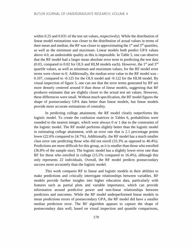
within 0.25 and 0.031 of the test set values, respectively). While the distribution of linear model estimations was closer to the distribution of actual values in terms of their mean and median, the RF was closer to approximating the 1st and 3rd quartiles, as well as the minimum and maximum. Linear models both predict GPA values above 4.0, an undesirable quality as this is impossible. In Table 5, one can observe that the RF model had a larger mean absolute error term in predicting the test data (0.03, compared to 0.02 for OLS and HLM models each). However, the 1st and 3rd quartile values, as well as minimum and maximum values, for the RF model error terms were closer to 0. Additionally, the median error value in the RF model was -0.107, compared to -0.125 for the OLS model and -0.122 for the HLM model. By visual inspection of figure 5, one can see that the error terms generated by RF are more densely centered around 0 than those of linear models, suggesting that RF produces estimates that are slightly closer to the actual test set values. However, these differences were small. Without much specification, the RF model figures the shape of postsecondary GPA data better than linear models, but linear models provide more accurate estimations of centrality.

In predicting college attainment, the RF model clearly outperforms the logistic model. To create the confusion matrices in Tables 6, probabilities were rounded to the nearest integer, which were always 0 or 1 due to the constraints of the logistic model. The RF model performs slightly better than the logistic model in estimating college attainment, with an error rate that is 2.1 percentage points lower (22.6% compared to 24.7%). Additionally, the RF model has a much smaller class error rate predicting those who did not enroll (33.3% as opposed to 40.4%). Predictions are more difficult for this group, as it is smaller than those who enrolled (36.8% of the sample size). The logistic model has a slightly lower error rate than RF for those who enrolled in college (15.5% compared to 16.4%), although this only represents 22 individuals. Overall, the RF model predicts postsecondary success more accurately than the logistic model.

This work compares RF to linear and logistic models in their abilities to make predictions and critically interrogate relationships between variables. RF models provide further insights into higher education data, particularly with features such as partial plots and variable importance, which can provide information around predictive power and non-linear relationships between predictors and outcomes. While the RF model underperformed linear models in mean predictions errors of postsecondary GPA, the RF model did have a smaller median prediction error. The RF algorithm appears to capture the shape of postsecondary data well, based on visual inspection and quantile comparisons,


171

although linear models may perform slightly better for students with greater High School GPAs. While the logistic model predicts enrollees slightly better than the RF algorithm, overall RF is superior in terms of estimating college access. Although the RF model did not outperform the other models in every application, it offered distinct advantages and was generally preferable to linear and logistic models.

Conclusions

How can the Random Forest algorithm advance quantitative higher education scholarship?

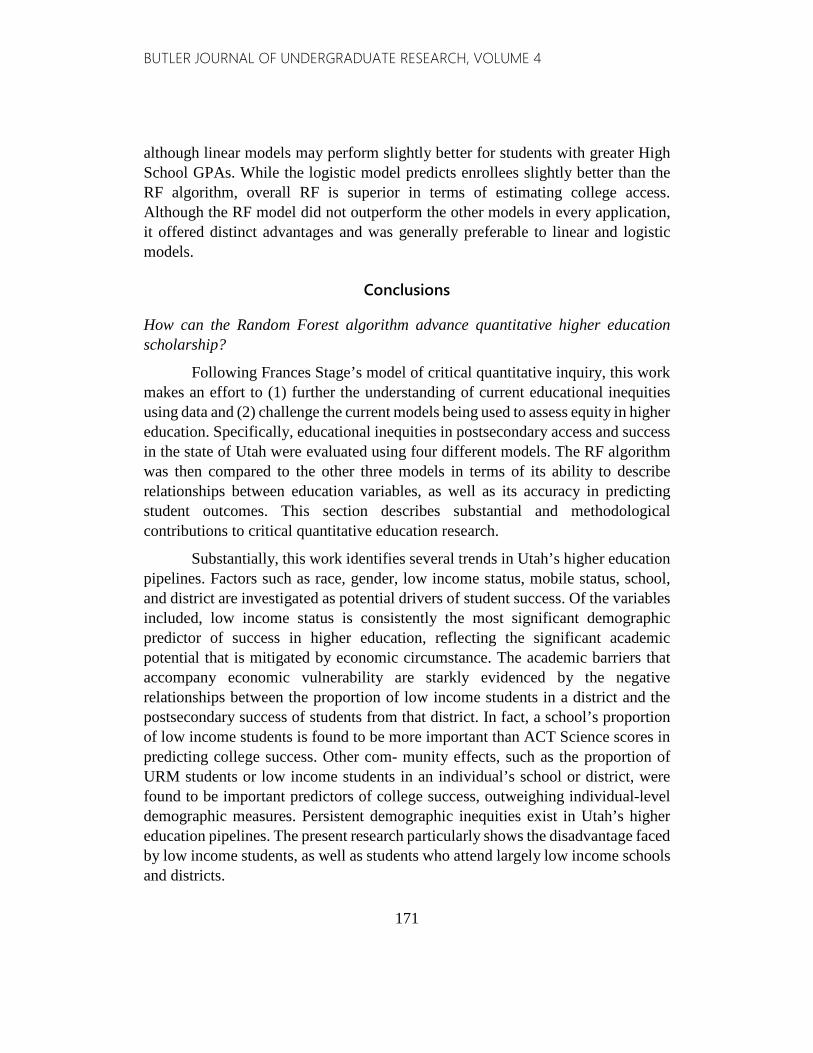
Following Frances Stage’s model of critical quantitative inquiry, this work makes an effort to (1) further the understanding of current educational inequities using data and (2) challenge the current models being used to assess equity in higher education. Specifically, educational inequities in postsecondary access and success in the state of Utah were evaluated using four different models. The RF algorithm was then compared to the other three models in terms of its ability to describe relationships between education variables, as well as its accuracy in predicting student outcomes. This section describes substantial and methodological contributions to critical quantitative education research.

Substantially, this work identifies several trends in Utah’s higher education pipelines. Factors such as race, gender, low income status, mobile status, school, and district are investigated as potential drivers of student success. Of the variables included, low income status is consistently the most significant demographic predictor of success in higher education, reflecting the significant academic potential that is mitigated by economic circumstance. The academic barriers that accompany economic vulnerability are starkly evidenced by the negative relationships between the proportion of low income students in a district and the postsecondary success of students from that district. In fact, a school’s proportion of low income students is found to be more important than ACT Science scores in predicting college success. Other community effects, such as the proportion of URM students or low income students in an individual’s school or district, were found to be important predictors of college success, outweighing individual-level demographic measures. Persistent demographic inequities exist in Utah’s higher education pipelines. The present research particularly shows the disadvantage faced by low income students, as well as students who attend largely low income schools and districts.


172

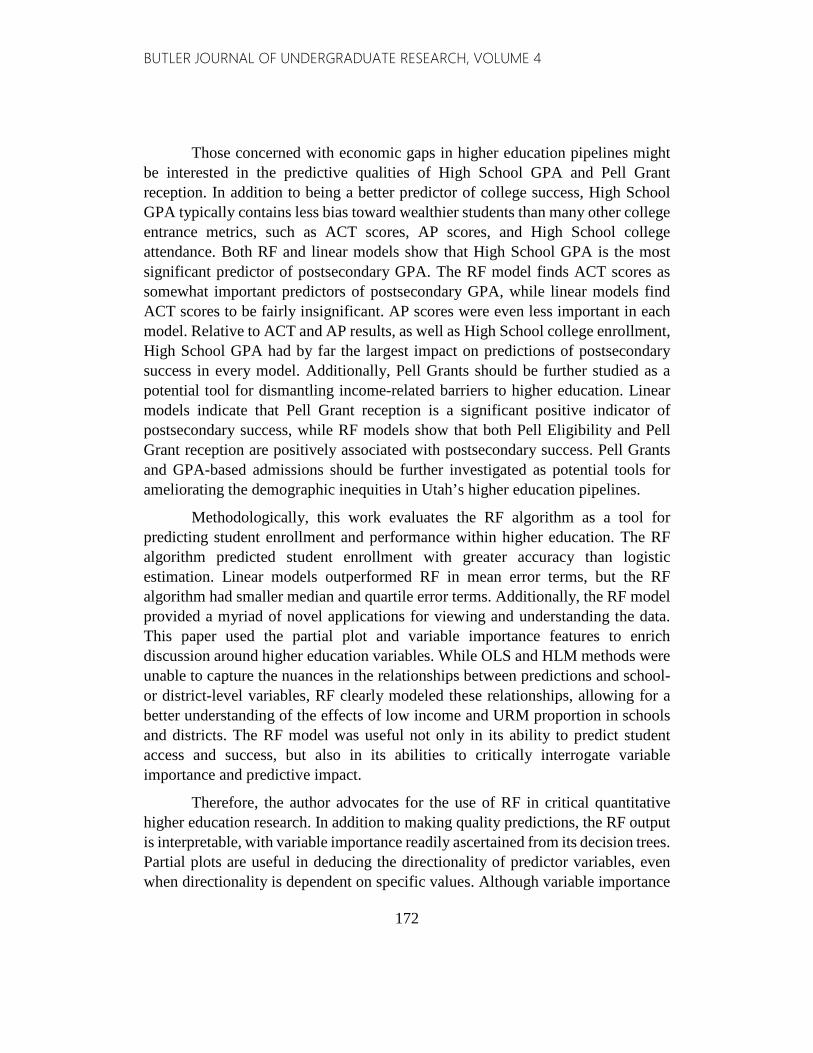
Those concerned with economic gaps in higher education pipelines might be interested in the predictive qualities of High School GPA and Pell Grant reception. In addition to being a better predictor of college success, High School GPA typically contains less bias toward wealthier students than many other college entrance metrics, such as ACT scores, AP scores, and High School college attendance. Both RF and linear models show that High School GPA is the most significant predictor of postsecondary GPA. The RF model finds ACT scores as somewhat important predictors of postsecondary GPA, while linear models find ACT scores to be fairly insignificant. AP scores were even less important in each model. Relative to ACT and AP results, as well as High School college enrollment, High School GPA had by far the largest impact on predictions of postsecondary success in every model. Additionally, Pell Grants should be further studied as a potential tool for dismantling income-related barriers to higher education. Linear models indicate that Pell Grant reception is a significant positive indicator of postsecondary success, while RF models show that both Pell Eligibility and Pell Grant reception are positively associated with postsecondary success. Pell Grants and GPA-based admissions should be further investigated as potential tools for ameliorating the demographic inequities in Utah’s higher education pipelines.

Methodologically, this work evaluates the RF algorithm as a tool for predicting student enrollment and performance within higher education. The RF algorithm predicted student enrollment with greater accuracy than logistic estimation. Linear models outperformed RF in mean error terms, but the RF algorithm had smaller median and quartile error terms. Additionally, the RF model provided a myriad of novel applications for viewing and understanding the data. This paper used the partial plot and variable importance features to enrich discussion around higher education variables. While OLS and HLM methods were unable to capture the nuances in the relationships between predictions and school- or district-level variables, RF clearly modeled these relationships, allowing for a better understanding of the effects of low income and URM proportion in schools and districts. The RF model was useful not only in its ability to predict student access and success, but also in its abilities to critically interrogate variable importance and predictive impact.

Therefore, the author advocates for the use of RF in critical quantitative higher education research. In addition to making quality predictions, the RF output is interpretable, with variable importance readily ascertained from its decision trees. Partial plots are useful in deducing the directionality of predictor variables, even when directionality is dependent on specific values. Although variable importance


173

plots and partial plots may stand alone, it is beneficial to compare such results with linear model coefficients.

While empirical in nature, RF results are not meant to be utilized as objective measures of reality. Instead, the algorithm provides information around student experiences, information which can be used to supplement the results of other models and give researchers a broader depiction of intricate relationships between predictors and outcomes. Critical quantitative studies on higher education stand to benefit from the RF algorithm’s novel prediction framework, accurate predictions, detail in describing predictive importance, and emphasis on interpretation.

Within the field of critical quantitative higher education, interpretation of results is widely considered the most important part of the research process. The RF model contributes new interpretations of student data to the field of critical quantitative research in higher education, some of which were not possible with linear or logistic models. Using the RF model, non-linear changes in predictive power can be viewed, allowing one to better grasp the effects of changes to individual variables on predicted outcomes. Variable importance can be understood in terms of out of bag errors, which are fundamentally different than traditional significance tests.

A second tenet to critical quantitative research is that it challenges previous work. Throughout this work, RF models contradict linear and logistic models’ conclusions around issues such as predictive directionality and variable significance or importance.

Lastly, critical research is motivated by the desire to change society. This work identifies GPA-based admissions and Pell Grants as potential tools for critically improving student access and success. Works that evaluate the use of such tools, and leaders who implement such policies, will inevitably change the structure of higher education. This work’s methodological and substantial findings are intended to expand the possibility of equitable education systems, as well as the notion that education pipelines might be advanced with quantitative design. Future studies comparing the efficacy of predictive algorithms and interpreting results critically to describe postsecondary pipelines will further current conceptions of equity within postsecondary education.


174

References

Allison, P. D. (2009). Missing data. Thousand Oaks, CA: Sage.

Beede, D. N., Julian, T. A., Langdon, D., Mckittrick, G., Khan, B., & Doms, M. E. (2011). Women in STEM: A Gender Gap to Innovation. SSRN Electronic Journal. doi:10.2139/ssrn.1964782

Bell, A., & Jones, K. (2014). Explaining Fixed Effects: Random Effects Modeling of Time-Series Cross-Sectional and Panel Data. Political Science Research and Methods, 3(01), 133-153. doi:10.1017/psrm.2014.7

Bensimon, E. M., & Bishop, R. (2012). Introduction: Why "Critical"? The Need for New Ways of Knowing. The Review of Higher Education, 36(1S), 1-7. doi:10.1353/rhe.2012.0046

Blanch, A., & Aluja, A. (2013). A regression tree of the aptitudes, personality, and academic performance relationship. Personality and Individual Differences, 54(6), 703-708. doi:10.1016/j.paid.2012.11.032

Breiman, L. (1998). Classification and regression trees. Boca Raton: Chapman and Hall/CRC.

---. (2001). Machine Learning, 45(1), 5-32. doi:10.1023/a:1010933404324

---. (2002). Manual on setting up, using, and understanding Random Forests (1st ed., Vol. 3). Berkeley, CA: Statistics Department, University of California Berkeley.

Brown, I., & Mues, C. (2012). An experimental comparison of classification algorithms for imbalanced credit scoring data sets. Expert Systems with Applications, 39(3), 3446-3453. doi:10.1016/j.eswa.2011.09.033

Burtless, G. T. (1996). Does money matter?: The effect of school resources on student achievement and adult success. Washington (D.C.): Brookings institution.

Cabrera, A. F. (1994). Logistic regression analysis in higher education. In Higher education: Handbook of theory and research (Vol. 10, pp. 225-256).


175

Chambers, T. V. (2009). "The Receivement Gap": School Tracking Policies and the Fallacy of the Achievement Gap. The Journal of Negro Education, 417-431.

Chen, X., & Weko, T. (2009). Stats in brief: Students who study science, technology, engineering, and mathematics (STEM) in postsecondary education (Rep. No. NCES 2009-161). Washington, DC: National Center for Education Statistics, Institute of Education Sciences, US Department of Education.

Chetty, R., Friedman, J. N., Saez, E., Turner, N., & Yagan, D. (n.d.). Mobility Report Cards: The Role of Colleges in Intergenerational Mobility (Tech.). Retrieved July, 2017, from Internal Revenue Servce website: http://www.equality-of-opportunity.org/papers/coll_mrc_paper.pdf

Cortez, P., & Goncalves Silva, A. (2008). Using data mining to predict secondary school student performance [Scholarly project]. Retrieved from http://www3.dsi.uminho.pt/pcortez/student.pdf

Daniel, B. (2014). Big Data and analytics in higher education: Opportunities and challenges. British Journal of Educational Technology, 46(5), 904-920. doi:10.1111/bjet.12230

Díaz-Uriarte, R., & Alvarez De Andres, S. (2006). Gene selection and classification of microarray data using random forest. BMC Bioinformatics, 7(1), 3.

Dismuke, C., & Lindrooth, R. (2006). Ordinary least squares. Methods and Designs for Outcomes Research, 93, 93-104.

Dowd, A. (2007). Community Colleges as Gateways and Gatekeepers: Moving beyond the Access "Saga" toward Outcome Equity. Harvard Educational Review, 77(4), 407-419. doi:10.17763/haer.77.4.1233g31741157227

Frankenberg, E., & Orfield, G. (2012). The resegregation of suburban schools: A hidden crisis in American education. Cambridge, MA: Harvard Education Press.

Garces, L. M., & Cogburn, C. D. (2015). Beyond Declines in Student Body Diversity. American Educational Research Journal, 52(5), 828-860. doi:10.3102/0002831215594878.


176

Garner, C. L., & Raudenbush, S. W. (1991). Neighborhood Effects on Educational Attainment: A Multilevel Analysis. Sociology of Education, 64(4), 251. doi:10.2307/2112706.

Geiser, S., & Santelices, M. V. (2007). Validity of High-School Grades in Predicting Student Success beyond the Freshman Year: High-School Record vs. Standardized Tests as Indicators of Four-Year College Outcomes [Scholarly project]. In Center for Studies in Higher Education. Retrieved from https://cshe.berkeley.edu/sites/default/files/publications/rops.geiser._sat_6.13.07.pdf.

Gerber, T. P., & Schaefer, D. R. (2004). Horizontal Stratification of Higher Education in Russia: Trends, Gender Differences, and Labor Market Outcomes. Sociology of Education, 77(1), 32-59. doi:10.1177/003804070407700102

Geurts, P., Irrthum, A., & Wehenkel, L. (2009). Supervised learning with decision tree-based methods in computational and systems biology. Molecular BioSystems, 5(12), 1593. doi:10.1039/b907946g.

Golino, H. F., Gomes, C. M., & Andrade, D. (2014). Predicting Academic Achievement of High-School Students Using Machine Learning. Psychology, 05(18), 2046-2057. doi:10.4236/psych.2014.518207.

Golino, H. F., & Gomes, C. M. (2014). Visualizing Random Forest’s Prediction Results. Psychology, 05(19), 2084-2098. doi:10.4236/psych.2014.519211.

Hardman, J., Paucar-Caceres, A., & Fielding, A. (2012). Predicting Students Progression in Higher Education by Using the Random Forest Algorithm. Systems Research and Behavioral Science, 30(2), 194-203. doi:10.1002/sres.2130.

Hardman, J., Paucar-Caceres, A., Urquhuart, C., & Fielding, A. (2010). Predicting Students Progression Using Existing University Datasets: A Random Forest Application. In AMCIS Proceedings. Retrieved from https://aisel.aisnet.org/amcis2010/272/.

Hastie, T., Tibshirani, R., & Friedman, J. H. (2017). The elements of statistical learning: Data mining, inference, and prediction. New York, NY, USA: Springer.


177

Honaker, J., King, G., & Blackwell, M. (2011). Amelia II: A program for missing data. Journal of Statistical Software, 45(7), 1-47.

H., M, C., A., & C. (n.d.). The Missing "One-Offs": The Hidden Supply of High-Achieving, Low Income Students. Retrieved April 12, 2018, from http://www.nber.org/papers/w18586.

Hurtado, S. (2007). Linking Diversity with the Educational and Civic Missions of Higher Education. The Review of Higher Education, 30(2), 185-196. doi:10.1353/rhe.2006.0070.

Hurtado, S., Eagan, M. K., Cabrera, N. L., Lin, M. H., Park, J., & Lopez, M. (2007). Training Future Scientists: Predicting First-year Minority Student Participation in Health Science Research. Research in Higher Education, 49(2), 126-152. doi:10.1007/s11162-007-9068-1.

Hurtado, S., Cabrera, N. L., Lin, M. H., Arellano, L., & Espinosa, L. L. (2008). Diversifying Science: Underrepresented Student Experiences in Structured Research Programs. Research in Higher Education, 50(2), 189-214. doi:10.1007/s11162-008-9114-7.

Immigration, U.S. and Customs Enforcement. (2012). Stem-Designated Degree Program List. Retrieved from https://www.ice.gov/sites/default/files/documents/Document/2014/stem-list.pdf.

Iturriaga, F. J., & Sanz, I. P. (2015). Bankruptcy visualization and prediction using neural networks: A study of U.S. commercial banks. Expert Systems with Applications, 42(6), 2857-2869. doi:10.1016/j.eswa.2014.11.025.

Jacobson, L., & Mokher, C. (2009). Pathways to Boosting the Earnings of Low-Income Students by Increasing their educational attainment (Rep.). Retrieved https://files.eric.ed.gov/fulltext/ED504078.pdf.

Karen, D. (2002). Changes in Access to Higher Education in the United States: 1980-1992. Sociology of Education,75(3), 191. doi:10.2307/3090265.

Kena, G., Hussar, W., McFarland, J., De Brey, C., Musu-Gillette, L., Wang, X., . . . Dunlop Velez, E. (2016). The Condition of Education 2016(Rep. No. NCES 2016-144). Retrieved https://files.eric.ed.gov/fulltext/ED565888.pdf.


178

Khaidem, L., Snehanshu, S., & Dev, S. R. (2016). Predicting the direction of stock market prices using random forest [Scholarly project]. Retrieved from https://arxiv.org/pdf/1605.00003.pdf

Kincheloe, J. L., Mclaren, P., & Steinberg, S. R. (2012). Critical pedagogy and qualitative research: Moving to the bricolage. In Critical qualitative research reader (pp. 14-32). New York, NY: Peter Lang.

Kincheloe, J. L., & Mclaren, P. (2011). Rethinking Critical Theory and Qualitative Research. Key Works in Critical Pedagogy, 285-326. doi:10.1007/978-94-6091-397-6_23

Kirst, M., & Venezia, A. (2004). From high school to college: Improving opportunities for student success. San Francisco, CA: Jossey-Bass..

Liaw, A., & Wiener, M. (2014). Package 'randomForest': Breiman and Cutler's random forests for classification and regression. R Development Core Team. 4. 6-10.

Liaw, A., & Wiener, M. (2001). Classification and Regression by RandomForest. Forest. 23. Mihelich, J., & Storrs, D. (2003). Higher Education and the Negotiated Process of Hegemony. Gender & Society, 17(3), 404-422. doi:10.1177/0891243203017003007.

Naeem, S., Hylands, P., & Barlow, D. (2012). Construction of an Indonesian herbal constituents database and its use in Random Forest modelling in a search for inhibitors of aldose reductase. Bioorganic & Medicinal Chemistry, 20(3), 1251-1258. doi:10.1016/j.bmc.2011.12.033.

Noble, J. P., & Sawyer, R. L. (2004). “Is high school GPA better than admission test scores for predicting academic success in college. College and University, 79(4), 17.

Perna, L. W., & Swail, W. S. (2001). Pre-college outreach and early intervention. Thought & Action, 17(1), 99.

Quinlan, J. R. (1993). C4.5: Programs for machine learning. San Mateo Calif: Morgan Kaufmann Random Forests Leo Breiman and Adele Cutler. (n.d.). Retrieved April 12, 2018, from https://www.stat.berkeley.edu/~breiman/RandomForests/Raudenbush, Stephen and Anthony S Bryk. “A hierarchical model for studying school effects”. Sociology of education (1986), pp. 1–17.


179

Raudenbush, S. W., & Bryk, A. S. (2002). Hierarchical linear models: Applications and data analysis methods. Thousand Oaks (California): Sage.

Reardon, S.F. (2015). School Segregation and Racial Academic Achievement Gaps (CEPA Working Paper No.15-12). Retrieved from Stanford Center for Education Policy Analysis: http://cepa.stanford.edu/wp15-12”. RSF (2016).

Sackett, P. R., Kuncel, N. R., Arneson, J. J., Cooper, S. R., & Waters, S. D. (2009). Does socioeconomic status explain the relationship between admissions tests and post-secondary academic performance? Psychological Bulletin, 135(1), 1-22. doi:10.1037/a0013978

Sawyer, R. (2013). Beyond Correlations: Usefulness of High School GPA and Test Scores in Making College Admissions Decisions. Applied Measurement in Education, 26(2), 89-112. doi:10.1080/08957347.2013.765433.

Skogli, E. W., Teicher, M. H., Andersen, P. N., Hovik, K. T., & Øie, M. (2013). ADHD in girls and boys – gender differences in co-existing symptoms and executive function measures. BMC Psychiatry, 13(1). doi:10.1186/1471-244x-13-298.

Slater, S., Joksimović, S., Kovanovic, V., Baker, R. S., & Gasevic, D. (2016). Tools for educational data mining: A review. Journal of Educational and Behavioral Statistics, 42(1), 85-106. doi:10.3102/1076998616666808.

Snijders, T., & Bosker, R. (1999). Multilevel analysis: An introduction to basic and applied multilevel analysis. Sage Publications.

Stage, F. K. (2007), Answering critical questions using quantitative data. New Directions for Institutional Research, 2007: 5-16. doi:10.1002/ir.200.

Steiger, J. H. (2009). The 3-Level HLM Model. Retrieved from http://www.statpower.net/Content/MLRM/Lecture Slides/HLM3.pdf

Superby, J., Vandamme, J., & Meskens, N. (2006). Determination of factors influencing the achievement of the first-year university students using data mining methods. In Workshop on Educational Data Mining (Vol. 32, p. 234).

Svetnik, V., Liaw, A., Tong, C., Culberson, J. C., Sheridan, R. P., & Feuston, B. P. (2003). Random Forest: A Classification and Regression Tool for Compound Classification and QSAR Modeling. Journal of Chemical


180

Information and Computer Sciences, 43(6), 1947-1958. doi:10.1021/ci034160g.

Turley, R. N. (2009). College Proximity: Mapping Access to Opportunity. Sociology of Education, 82(2), 126-146. doi:10.1177/003804070908200202.

Wald, J. and Losen, D. J. (2003), Defining and redirecting a school‐to‐prison pipeline. New Directions for Youth Development, 2003: 9-15. doi:10.1002/yd.51

Wang, G., Hao, J., Ma, J., & Jiang, H. (2011). A comparative assessment of ensemble learning for credit scoring. Expert Systems with Applications, 38(1), 223-230. doi:10.1016/j.eswa.2010.06.048.

You, S., & Nguyen, J. (2012). Multilevel analysis of student pathways to higher education. Educational Psychology, 32(7), 860-882. doi:10.1080/01443410.2012.746640.

Zajacova, A., Lynch, S. M., & Espenshade, T. J. (2005). Self-efficacy, stress, and academic success in college. Research in Higher Education, 46(6), 677-706.

Documents

Using Random Forests to Describe Equity in Higher