This is a repository copy of Using ordered attitudinal indicators in a latent variable choice model: A study of the impact of security on rail travel behaviour.

White Rose Research Online URL for this paper:http://eprints.whiterose.ac.uk/43603/

Article:

Daly, AJ, Hess, S, Patruni, B et al. (2 more authors) (2012) Using ordered attitudinal indicators in a latent variable choice model: A study of the impact of security on rail travel behaviour. Transportation, 39 (2). 267 - 297 . ISSN 0049-4488

https://doi.org/10.1007/s11116-011-9351-z

eprints@whiterose.ac.ukhttps://eprints.whiterose.ac.uk/

Reuse

Unless indicated otherwise, fulltext items are protected by copyright with all rights reserved. The copyright exception in section 29 of the Copyright, Designs and Patents Act 1988 allows the making of a single copy solely for the purpose of non-commercial research or private study within the limits of fair dealing. The publisher or other rights-holder may allow further reproduction and re-use of this version - refer to the White Rose Research Online record for this item. Where records identify the publisher as the copyright holder, users can verify any specific terms of use on the publisher’s website.

Takedown

If you consider content in White Rose Research Online to be in breach of UK law, please notify us by emailing eprints@whiterose.ac.uk including the URL of the record and the reason for the withdrawal request.

1

Using ordered attitudinal indicators in a latent variable

choice model: A study of the impact of security on rail travel

behaviour

Andrew Daly*1,2

, Stephane Hess2, Bhanu Patruni

1, Dimitris Potoglou

1,3, Charlene Rohr

+1

* authors listed alphabetically + corresponding author 1Rand Europe, Westbrook Centre, Milton Road, CB4 1YG, Cambridge, UK

2Institute of Transport Studies, University of Leeds, Leeds, UK

3OTB Research Institute, Delft University of Technology, Delft, Netherlands

Abstract

There is growing interest in the use of models that recognise the role of individuals' attitudes and perceptions

in choice behaviour. Rather than relying on simple linear approaches or a potentially bias-inducing

deterministic approach based on incorporating stated attitudinal indicators directly in the choice model,

researchers have recently recognised the latent nature of attitudes. The uptake of such latent attitude models

in applied work has however been slow, while a number of overly simplistic assumptions are also commonly

made. In this paper, we present an application of jointly estimated attitudinal and choice models to a real

world transport study, looking at the role of latent attitudes in a rail travel context. Our results show the

impact that concern with privacy, liberty and security, and distrust of business, technology and authority have

on the desire for rail travel in the face of increased security measures, as well as for universal security checks.

Alongside demonstrating the applicability of the model in applied work, we also address a number of

theoretical issues. We first show the equivalence of two different normalisations discussed in the literature.

Unlike many other latent attitude studies, we explicitly recognise the repeated choice nature of the data.

Finally, the main methodological contribution comes in replacing the typically used continuous model for

attitudinal response by an ordered logit structure which more correctly accounts for the ordinal nature of the

indicators.

Keywords: attitudes; latent variables model; discrete choice; stated choice; privacy, security and

liberty; rail travel

1. Introduction

Standard discrete choice models represent the decision making process as an interaction between

measured attributes of the alternatives (and possibly of the decision maker) and estimated

sensitivities of the decision maker. This simplified approach has been heavily criticised by

behavioural scientists as it often neglects important idiosyncratic aspects of behaviour and cannot

deal with apparently irrational decisions (see for example Gärling 1998). Meanwhile, researchers

have increasingly recognised that decision makers differ significantly from one another, and the

treatment of differences in sensitivities (and hence choices) across individual decision makers is one

of the main areas of interest in choice modelling. While these differences can often be directly linked

to socio-demographic characteristics such as age and income, a case has repeatedly been made that

underlying attitudes and perceptions may be equally important predictors for these differences,

2

notwithstanding that these attitudes and perceptions may once again be explained by socio-

demographic characteristics.

The main issue facing analysts in this context is that while socio-demographic characteristics are

directly measurable, the same does not apply to underlying perceptions and attitudes, which are

unobserved in the same way that respondent specific sensitivities are not known. In other words,

these latent variables are factors that cannot be observed directly; rather, they can at best be

inferred from other variables called indicators (Golob 2001; Choo and Mokhtarian 2004). Here,

psychometric indicators (typically on a Likert scale) such as responses to survey questions about

attitudes, perceptions or decision-making protocols are used as manifestations of the underlying

latent attitudes.

We specifically define attitudes and perceptions as follows. Attitudes reflect latent variables

corresponding to the characteristics of the decision-ﾏ;ﾆWヴ ;ﾐS ヴWaﾉWIデ ｷﾐSｷ┗ｷS┌;ﾉゲげ ﾐWWSゲが ┗;ﾉ┌Wゲが tastes, and capabilities. Attitudes are formed over time and are affected by experience and external

factors including socio-economic characteristics (Walker and Ben-Akiva 2002). Perceptions measure

デｴW ｷﾐSｷ┗ｷS┌;ﾉげゲ Iﾗｪﾐｷデｷ┗W I;ヮ;Iｷデ┞ デﾗ ヴWヮヴWゲWﾐデ ;ﾐS W┗;ﾉ┌;デW デｴW ﾉW┗Wﾉゲ ﾗa デｴW ;デデヴｷH┌デWゲ ﾗa SｷaaWヴWﾐデ alternatives. Perceptions are relevant because the choice process depends on how attribute levels

are perceived by the individual beliefs of a specific consumer (Bolduc and Daziano 2008).

The focus of this paper is specifically on the incorporation of individuals' attitudes in discrete choice

models. Latent attitudes may play as much of a role in shaping choice as the attributes of the

alternatives (Ashok et al. 2002). Therefore, extending choice models to include latent attitudes can

lead to a better understanding of the choice processes. Moreover, it is expected that these

enhanced models could provide greater explanatory power (Bolduc et al. 2005; Temme et al. 2008).

Early efforts used Structural Equations Models for jointly modelling choices and attitudes. An

excellent review of this work is given by Golob (2003). However, at the time of that paper there

remained severe software limitations, which implied that both choice variables and attitudinal

indicators could be modelled only by linear regression techniques (e.g. as in Golob et al. (1997)). This

approach, which is in any case limited to binary choice, must be considered methodologically

unsatisfactory.

The use of attitudes in discrete choice models, in particular, is not new, and a number of different

approaches have been used in past work. The most direct approach relies on using choice models

with indicators. In this case, indicators of the underlying latent variable are treated as error-free

explanatory predictors of choice (see Figure 1a). In other words, rather than correctly treating

indicators as functions of underlying attitudes, they are treated as direct measures of the attitudes.

The main disadvantages of this approach are that strong agreement with an attitudinal statement

does not necessarily translate into a causal relationship with choice. Additionally, indicators are

highly dependent on the phrasing of the survey, and furthermore they are not available for

forecasting. Incorporating the indicators of latent variables as explanatory variables also ignores the

fact that latent variables contain measurement error, and can thus lead to inconsistent estimates

(Ashok et al. 2002). Finally, indicators are arguably correlated with the error of the choice model, i.e.

デｴWヴW ;ヴW ┌ﾐﾗHゲWヴ┗WS WaaWIデゲ デｴ;デ ｷﾐaﾉ┌WﾐIW Hﾗデｴ ; ヴWゲヮﾗﾐSWﾐデげゲ IｴﾗｷIW ;ﾐS ｴｷゲっｴWヴ ヴWゲヮﾗﾐゲWゲ デﾗ indicator questions. This thus creates a risk of endogeneity bias.

An alternative is a sequential estimation approach using factor analysis or structural equation

modelling (SEM) for the latent variable component and discrete choice models for the choice

3

component of the model. Factor analysis can be either confirmatory (CFA) or confirmatory with

covariates - that is a Multiple Indicator Multiple Cause (MIMIC) model. The factor analysis approach

involves analysis of the interrelationships between attitudinal indicators and a statistical procedure

that transforms the correlated indicators into a smaller group of uncorrelated (latent) variables

called principal components or factors. This procedure requires a single measurement equation. On

the other hand, SEM involves two parts: a measurement model and a structural model. SEMs

capture three relationships: the relationship among factors (latent variables), the relationship

among observed variables and the relationship between factors and observed variables that are not

factor indicators. As a next step, the latent variables are entered in the utility equations (see Figure

1b) of the choice models. The latent variables contain measurement error, and in order to obtain

consistent estimates, the choice probability must be integrated over the distribution of latent

variables, where the distribution of the factors is obtained from the factor analysis model. This

method recognises that both the choice and the response to the indicator questions are driven by

the same underlying latent variable. The key disadvantage of this approach is that the latent

estimates are inefficient, i.e. they are derived from the attitudinal information only and do not take

account of actual choices that the respondent has made (see for example Morikawa et al. (2002)).

Past work has also made use of internal market analysis, in which both latent attributes of the

alternatives and consumer preferences are inferred from preference or choice data. In this

restrictive approach (Figure 1c), the observed choices are the only indicators used, and therefore the

latent attributes are alternative specific and do not vary among individuals in a market segment (see

for example: Elrod, (1988); Elrod and Keane, (1995)).

[Figure 1, about here]

With a view to improving on the above methods, recent research efforts have led to the formulation

of combined model structure offering a general treatment of the inclusion of latent variables in

discrete choice models. In particular, this model framework is comprised of two components: a

discrete choice model and a latent variable model (Figure 2). In the remainder of this paper, we will

make use of the name coined for this structure by Bolduc et al. (2005), who refer to it as the

Integrated Choice and Latent Variable (ICLV) model, although this term postdates some of the earlier

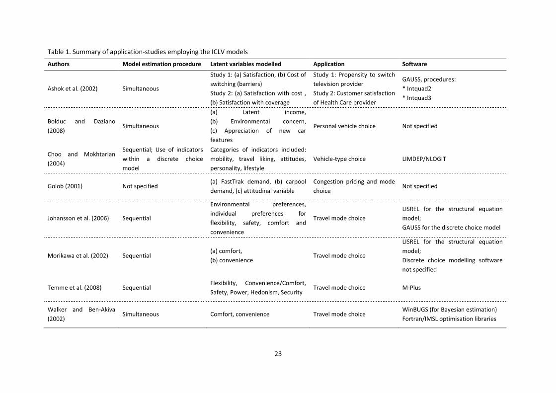
developments. Before proceeding to a more detailed discussion of the ICLV structure, Table 1

provides a summary of previous efforts to incorporate latent variables in discrete choice models.

[Figure 2, about here]

[Table 1, about here]

The ICLV structure can add to the realism of the model because it explicitly describes how

perceptions and attitudes affect choices, as well as using information on observed choices to inform

the estimation of the latent attitudinal variables (as opposed to simply using the latent variables as

input into the choice model). In the discrete choice model componentが ;ﾉデWヴﾐ;デｷ┗Wゲげ ┌デｷﾉｷデｷWゲ ﾏ;┞ depend on both observed and latent explanatory variables of the options and decision makers. At

the same time, these latent variables help explain the responses to observed indicators (that

represent manifestations of the latent constructs), while possibly also being functions of explanatory

variables (Johansson et al. 2006). In terms of modelling, the latent variables are viewed as structural

variables which are related to other variables through a structural latent variable model framework1

(Bolduc et al. 2005). The latent-variable part of the model captures the relationships between latent

1 A linear structural relation (LISREL) model is a special case.

4

variables and MIMIC-type models simultaneously, in which observed exogenous variables influence

the latent variables (Temme et al. 2008).

The structural latent variable model formulation incorporates a sub-model that uses the latent

variables as explanatory variables in a model in which the dependent variables are answers to

questions of a survey (the indicators). The complete model is composed of a group of structural

equations (structural model) and a group of measurement relationships (measurement model). The

structural model describes the latent variables in terms of observable exogenous variables as well as

specifying the utility functions on the basis of observable exogenous variables and the latent

variables. The measurement model links latent variables to the indicators. Estimation of the

parameters in the full system can be done sequentially (see Ashok et al. 2002; Johansson et al. 2006;

Temme et al. 2008) or jointly, i.e. full information (see Bolduc et al. 2005; Morikawa et al. 2002;

Walker and Ben-Akiva 2002). Sequential estimation provides consistency while joint (simultaneous)

estimation adds efficiency (Bolduc et al. 2005).

Despite their inherent appeal, latent attitude models have thus far only been used rather rarely in

applied transport research (and elsewhere). One possible reason for this is the way in which the

theoretical work has been spread across numerous disciplines. The first aim of the present paper is

thus to provide a comprehensive overview of the methodological framework. Next, this paper makes

a methodological extension to previous work on integrated choice and latent variable (ICLV) models

by Ben Akiva et al. (1999) and Bolduc et al. (2005) by incorporating ordered-logit choice models for

the measurement equations of the attitudinal variables. Seemingly unlike much other latent variable

choice modelling work, we also explicitly account for the repeated choice nature of the (stated

preference) data. As an additional contribution, we present some evidence from a comparison of

two commonly used normalisations of ICLV models. In line with a small but growing subset of other

studies, we use simultaneous rather than sequential estimation. The empirical application of the

models is also novel, looking at the use of attitudinal variables in the context of a stated choice

survey on UK ヴ;ｷﾉ ヮ;ゲゲWﾐｪWヴゲげ trade-offs across privacy, liberty and security.

The remainder of this paper is organised as follows. The following section presents the

methodological framework used in the present work, including the extension to an ordered model

for the attitudinal responses. We then present the choice context used for the empirical example,

with model specification and estimation results being discussed next. Finally, we present the

conclusions of the work.

2. Methodology

2.1 Outline of the model

The situation we seek to model is one in which we observe stated or actual choices by surveying

respondents who also record responses to attitudinal questions. We hypothesise that both choice

and attitudinal responses are influenced by latent variables and we seek to model the choice and

attitudinal responses together to give more insight into the processes that motivate respondentsげ behaviour. Three sets of relationships therefore have to be defined, as follows. We note that in the

following specification we have not used an index for the respondent as it is not necessary for the

present discussion. However, it should be understood that all of the variables, except the

parameters to be estimated, are in principle specific to respondents.

5

Choice among the set J of alternatives is modelled by assuming travellers maximise utility, which

we assume to be linear in parameters:

JjZcYaXUk jjjj |)(maxarg (1)

Here, k refers to the chosen alternative, Xj is a vector of M attributes2 of alternative j, while Z is a

vector of L latent variables. The vector a measures the impact of the attributes in Xj on the utility of

alternative j. The impact of the latent variables on the utility of alternative j is controlled by Yj. Here,

),( LNYj is a matrix of variables indicating whether a given coefficient in the vector c applies to a

given latent variable in the utility function for alternative j. The entries in the matrix Yj may be

dummies or data values for socio-economic or alternative attributes or combinations of these, and

we have N different interactions in c. As an example, if the latent attitude p is to be interacted with

the sensitivity to a given attribute, with this interaction captured in the qth

element in c, then Yj,q,p

would be given by the value of that attribute for alternative j. If, on the other hand, the qth

element

was to capture the absolute impact of the pth

latent variable on the utility of alternative r (i.e. on its

alternative specific constant), then Yr,q,p would be equal to 1, and Yj,q,p would be equal to 0 for all ũтƌ.

Finally, j is a random component of the utility function. The scale of U is fixed by the

distributional assumptions made for , which are discussed below. The coefficients a and c require

estimation, together with any parameters needed to define the distribution of .

Attitudinal responses are modelled by a series of relationships ﾆﾐﾗ┘ﾐ ;ゲ デｴW けﾏW;ゲ┌ヴWﾏWﾐデげ equations, which the literature generally assumes to be linear,:

ssss Zdy (2)

Here, ys gives the observed response to the sth

attitudinal indicator (out of S). The impact of the

latent variables on the value of the indicator is given by the estimated vector of parameters ds

(specific to a given indicator), which may contain zero values when some latent variables are

deemed (or found) not to have any impact on a given indicator. The reason for making d specific to a

given indicator s is that while a and c in Equation 1 will have some elements shared across

alternatives, the impacts of the latent variables in the measurement equations will almost surely be

different across indicators. Finally, ɸs gives the random component of the attitudinal response. Each

of these equations will require a constant ɷs, because y is measured on an arbitrary scale (e.g. 1-5);

alternatively, the mean value of each ys may be subtracted from the nominal values, so that the

mean does not have to be estimated with the other parameters.

Latent variables ;ヴW ;ゲゲ┌ﾏWS デﾗ HW SWデWヴﾏｷﾐWS H┞ ; ゲWヴｷWゲ ﾗa けゲデヴ┌Iデ┌ヴ;ﾉげ ヴWﾉ;デｷﾗﾐゲｴｷヮゲが ;ﾉゲﾗ ;ゲゲ┌ﾏWS to be linear:

lll bWZ (3)

Here, ),( QLW are socio-economic variables relating to the latent variables, where it is necessary to

specify sufficient unit values in W so that there is effectively a constant in the equation for each Z ;

this avoids Z being determined by the arbitrary measurement of W . The impact of the elements in

the vector Wl on the latent variable Zl is estimated by the vector b, while

)(L is the error in the

latent variable equation.

2 For alternatives that can be labelled it would be usual to include sufficient unit values in X to allow

appropriate constants to be estimated. That is, X(J,M) represents the measured variables, both alternative-specific and socio-economic (and compounds of these) that affect choice.

6

The use of this model entails the estimation of a number of vectors of parameters, namely:

a(M), giving the impact of measured attributes on utilities;

b(Q), giving the impact of socio-demographics on latent variables;

c(N), giving the impact of latent variables on utilities, where the N rows allow for example

for different interactions with different attributes, as well as alternative specific impacts;

and

ds(L), giving the impact of latent variables on the indicators, with a different d for each

indicator.

One final but important point needs discussing, namely the normalisation of the scale for the

measurement equations (i.e. Equation 2). Two normalisations have been discussed in the literature.

In the approach taken by Ben-Akiva et al. (1999), the scale of Z is fixed by constraints on the

elements in ds. Specifically, combining ds, with s=1,...S into a matrix d(S,L), the impact of each of the

latent variables is normalised for one of the attitudinal indicators, i.e. one of the non-zero values in

each of the L columns is normalised. The variance of then needs to be estimated. In the approach

taken by Bolduc et al. (2005), the variance of is normalised to 1, and all entries in d are

estimated. In either case the scale of , i.e. the standard deviation of the error in the measurement

equations, needs to be estimated. In theory, the two normalisations are equivalent, but to our

knowledge, this has not been shown in practice. We thus consider both of these normalisations in

the initial stages of the modelling.

2.2 Assumptions

The objective is to estimate the vectors of parameters dcba ,,, as well as the parameters of the

distributions of the random components ,, . Since we have required constants in the equations,

it is reasonable to assume that these random components have mean zero (or a standard mean

value). This means that we are concerned only with the covariance matrices of the random

components.

We therefore have to introduce three further parameters of the model to be estimated:

the covariance matrix of ;

the covariance matrix of ; and

the covariance matrix of .

We propose to estimate these three parameters along with dcba ,,, by maximum likelihood.

Further, it is reasonable to assume (at least in the first instance) that ,, are mutually

independent.

Assumption: ,, are mutually independent.

The three linear equations in the previous section represent three basic assumptions on which the

modelling is based. Generally, we are relatively happy with the assumptions of linearity relating to

utility U and the latent variables Z . The same cannot be said for the attitudinal indicators. Indeed,

the attitudinal responses y will usually be collected on a scale, for example from 1 to 5, and linear

regression is not a correct way to model such responses, although it is common even in advanced

literature (e.g. Bolduc et al., (2005); Ben-Akiva et al., 1999). For that representation, we would

7

assume that has a multivariate normal distribution3. This is reconsidered in the final part of this

section, where we discuss the use of ordered choice models to represent the attitudinal responses.

The error in the structural equation for the latent variables can most conveniently be defined to

have a multivariate normal distribution with covariance matrix . As discussed above, for the

Bolduc et al (2005) normalisation, is defined to have unit variance, because this defines the scale

of Z , but for the Ben-Akiva et al. (1999,2005) normalisation, the diagonal elements of will be

estimated. Again, we have not used off-diagonal elements in this matrix for the current paper, but

the notation leaves the possibility open.

It can clearly be seen already that the presence of the random component in the latent variables

(see Equation 3) will lead to random variations in sensitivities across respondents when latent

attitudes are interacted with measured attributes in the utility functions (Equation 1). The model

thus falls into the Mixed Logit family of structures. However, it should be noted that such random

variations can also be introduced independently of the latent variables by changing the variation of

to incorporate additional randomness net of the latent variables, i.e.

jjj (4)

where is i.i.d. type I extreme value (Gumbel) and has some other distribution, for example

multivariate normal. In this way, the model net of the latent variables Z is a mixed logit structure, as

in the recent work by Yañez et al. (2010), which is however based on sequential estimation. This can

clearly also be exploited to allow for correlations between alternatives (by allowing some elements

in to be shared by some alternatives). Similarly, it would however also be possible to specify the

underlying choice model to be a Nested Logit or other advanced nesting structure.

In the previous discussion, we have suggested that most often the random variables can be

considered to be independent, i.e. there are no off-diagonal elements. This feature simplifies the

analysis considerably. Bolduc et alく ヴWaWヴ デﾗ デｴWゲW ﾏ;デヴｷIWゲ ;ゲ さﾐ┌ｷゲ;ﾐIW ヮ;ヴ;ﾏWデWヴゲざく While this is a

specific technical term, it understates the importance of the parameters, which are quite interesting

from the point of view of understanding and predicting behaviour.

A convenient notation is to define x\ to be an nn* matrix whose off-diagonal elements are zero

and whose diagonal elements are given by the vector x of dimension n .

Assumptions: ,, are distributed multivariate normal and is i.i.d. type I extreme value

(Gumbel).

,, are diagonal matrices; this leads to:

h\ ,

g\ and

f\ ,

where hgf ,, are vectors of standard errors (to be estimated).

If we assume that the choices are independent of each other, then there are no further

complications. Indeed, if we have a single choice per respondent, the choice probability for given

values of Z and can be expressed as,

3 For the present study we have not introduced off-diagonal elements into the covariance matrix of the

distribution, allowing for correlation between different attitudinal responses, but the possibility of doing so is provided within the notation.

8

j jjj

kkk

ZcYaX

ZcYaXZkp

exp

exp),|(

,

(5)

owing to the type I extreme value (Gumbel) assumption made for . However, with repeated

observations from each individual, such as in Stated Choice experiments, the probability for the

sequence of choices Tkkk ,..1 , conditional on Z and , is given by:

tj jtjjt

ktkkt

ZcYaX

ZcYaXZkp

exp

exp),|(

,

(6)

where the added subscript t is for choice tasks.

In many models the values of and Z will not vary between the choice occasions t for an

individual and in those cases the notation could be simplified accordingly. To simplify the notation

for this paper we shall write the utility for alternative j in choice task t net of the type I extreme

value term as jjtjtjt ZcYaXV , where we thus assume that j stays constant across choice

tasks. The unconditional choice probability for either single or repeated choices can now be written

as:

)()(,|)( ZdFdFtjZcYaXVkpkP ZZ jjtjtjt (7)

where ZFF , are the distributions of Z, respectively and with the understanding that either a

single choice or a choice sequence can be represented by p (i.e. T is possibly equal to 1). This is a

Mixed Logit structure with the additional role for the latent variable Z . With repeated choice data

such as used in this paper, we use Equation (6) inside Equation (7); the integration is carried out at

the level of a sequence of choices (rather than individual choices). The correlation may be induced

by the formulation of but also, and specifically to the latent variable model, correlation is induced

by Z , both in its deterministic and its random components, with the same value for Z applying to all

choices for a given respondent.

2.3 Maximum Likelihood Estimation

The equation for the attitudinal indicators was given above as a linear regression

sss Zdy (8)

Since s is distributed normally with mean zero and standard error sg , the likelihood of the

observation of Sy , conditional on a value of Z , is proportional to

s

ss

ss g

Zdyn

gZyP

1)|( (9)

where n represents the standard normal (0, 1) frequency function:

2exp

2

1 2xxn

(10)

Further, the likelihood of the sequence of values Syyy ,..1 is given by the integral over Z of

the products of the likelihoods of the separate sy values

9

dZg

Zdyn

gyP

s

ss

Zs

s

1 (11)

The key step in developing the estimation procedure is that the likelihood of jointly observing choice

k and indicator y is given by the product of the likelihoods of each observation, i.e. the product of

the different choices, as well as the responses to the attitudinal questions. Because of the

assumptions we have made about independence, we can write

)()(1

,|, ZdFdFg

Zdyn

gtjZcYaXVkpykP ZZ

s

ss

ssjjtjtjt

(12)

With tjZcYaXVkp jjtjtjt ,| referring to a sequence of choices, each choice made by an

individual in the sequence is influenced by the same set of latent variables , thus inducing a

correlation between those choices. This is equivalent to the standard mixed logit approach of

allowing coefficient values (i.e. in effect random variations around the fixed values in a) to vary

across respondents but stay constant across choices for the same respondent. Such random

heterogeneity not linked to latent variables is also possible within this more general model

(accommodated in j ), but we have not used this possibility in the current study.

The above notation can be extended to take account of the structure of bWZ to give

)()()(1

,)(|, dFdF

g

bWdyn

gtjbWcYaXVkpykP

s

ss

ssjjtjtjt

(13)

If the matrices , had off-diagonal elements, then a Cholesky transformation would be necessary

to set up a sampling scheme to estimate the model, as described by Bolduc et al. (2005). However,

for the present paper the matrices have been assumed to be diagonal, with standard errors h for

and f for . Then we can write

)()()(1

)(|,

dNdNg

hbWdyn

gfhbWcYaXVkpykP

s

ss

ssjjjtjtjt

(14)

where

zdxxnzN )()( is the cumulative standard normal distribution and the integration is now

over independent standard normal variables , . We have to estimate hgfdcba ,,,,,, .

This integration can be made by setting up a simulation P~

of the likelihood in the usual way:

s

rss

ssr jrjrjtjtjt g

hbWdyn

gfhbWcYaXVkp

RykP

)(1)(|

1,

~ (15)

where R draws, indexed by r , are made of , from independent standard normal distributions.

Note that at each draw, all of the components of , are drawn. Maximisation of the simulated P~

then gives consistent estimates of the parameters hgfdcba ,,,,,, as required.

10

2.4 Attitudinal responses as ordered choices

A more sophisticated approach to the representation of the attitudinal variables is to treat the

responses as ordered choices. Recall that we supposed in the presentation above that the attitudes

of respondents could be modelled as random variables as in equation (16), which repeats equation

(2),

sss Zdy (16)

To apply ordered choices we treat the attitudes as latent variables x and model the probability that

the attitude x lies within a particular range to give the observed response y :

sss Zdx (17)

s

sj

s

sjs

s

sss g

Zd

g

Zddx

g

ZdxZjy

j

j

1

1

|Pr

(18)

where is the normalised frequency function for and is its cumulative form. For consistency

with equation (16) we might use the normal distribution in this role, but to reduce difficulty in

evaluating the function (e.g. to avoid excessive random sampling) it is effective to use the logistic

distribution, which has a closed cumulative form. Here, we acknowledge that more complex

specifications of ordered choice models exist then than the one used here (Greene and Hensher

2010); we have selected a simple model that incorporates the main effects while not unnecessarily

increasing model complexity.

Because we are no longer measuring attitudes on a fixed linear scale, but expressing them as falling

in arbitrary intervals on an undefined scale, we need to fix the (multiplicative) scale of x and this

can most naturally be done by taking a standard variance for , i.e. eliminating g in equation (18).

In estimating the values we may note that we have to estimate one fewer value than we have

possible responses. That is, if the attitudinal responses are on a five-point scale, we can take

0 , 5 and estimate the four intermediate values. Clearly we need to impose the

constraint that 1 jj . Moreover, we need to fix the (additive) scale of against x , which can

be done either by omitting constants from the equation for x or by including constants and setting

(e.g.) 01 .

The likelihood of the series of attitudinal responses can then be written

s sysy ZdZdZyss 1|Pr

, (19)

where ys gives the value observed for the sth

indicator.

By replacing Equation (11) by Equation (19), we get a new version of Equation (14), namely:

)()()(|, 1

dNdNZdZdfhbWcYaXVkpykPs sysyjjjtjtjt ss

(20)

Here, we have replaced the continuous specification for the indicator by an ordered specification,

and the ordered response model for the indicators is clearly still estimated jointly with the choice

model, as can be seen from Equation (20). Note that now we estimate the parameters

,,,,,, hfdcba . In this specification, we now combine a discrete model for choices with an

ordered model for indicators; this has some similarities to work looking at jointly modelling discrete

11

and ordered choices (e.g. Bhat & Guo (2007)), but in our case, the ordered component relates to the

attitudinal indicators, and there is also the additional latent variable component.

3. Case-study of rail travel in the UK

3.1 Stated Choice Experimental Design

The data for the models described in this paper come from a stated choice survey conducted to

examine trade-offs between policies influencing privacy and liberty in return for security

improvements (for details see Potoglou et al. (2010)). The rationale for using stated choice methods

デﾗ IﾗﾉﾉWIデ S;デ; ﾗﾐ ｷﾐSｷ┗ｷS┌;ﾉゲげ デヴ;SW-offs between policies influencing privacy, liberty and security is

the absence of data describing such trade-offs and choices from the real world. In particular, the aim

of the study is to examine individualsげ willingness to trade privacy or liberty against security

improvements, and to quantify these trade-offs in terms of willingness-to-pay (WTP) for a particular

security improvement. The research objective of the study, therefore, was to examine whether

security improvements concerning rail travel would be acceptable to individuals and what factors

are likely to influence individualsげ decisions when privacy, liberty and security may be in conflict.

Stated choice methods were judged to have the potential to provide useful insights in answering

such questions.

The alternative attributes and their levels for the choice experiments were defined through in-depth

interviews with data protection officials (Hosein 2008) and security officials (Clarke 2007; Clarke

2008), press articles (BBC 2006) and literature review research (Cozens et al. 2002; UK Dept. for

Transport 2008, 2006; Srinivasan et al. 2006). The trade-offs between alternatives involved three

main categories of relevant attributes: security improvements in terms of surveillance equipment

and presence of security personnel and security checks; potential benefits such as increased

likelihood that a terrorist plot may be disrupted and how things may be handled in case an incident

occurs, and travel related characteristics such as waiting time to pass through security and additional

cost to cover security improvements. The complete list of attributes and levels used in the choice

experiment is shown in Table 2.

[Table 2, about here]

The SC experiment was set in the context of choosing between three options describing situations

that the respondent may experience when travelling on the UK national rail network. Specifically,

respondents were asked to Imagine that you are making a journey using public transport, such as

on the national railway system. We would like you then to consider three ways in which you might

make this journey. These are described by different levels of security or privacy. As shown in Figure

3, an additional fourth option in the scenario allowed respondents to opt-out from choosing one of

the first three alternatives, stating, I would choose not to use the rail system under any of these

conditionsざ. Each alternative differed in terms of security measures, potential benefits from

improved security, and travel related characteristics.

[Figure 3, about here]

The large number of attributes and levels meant that a full factorial design was clearly not

appropriate, while a D-efficient design was judged to be inapplicable in the absence of reliable prior

estimates for model coefficients. For these reasons, we settled on a design that is nearly (although

not fully) orthogonal in its nature, and which excluded a number of unrealistic combinations. As an

12

example, security checks could not be performed using さMetal detector に X-rayざ if the waiting time

for the alternative was less than four minutes. Second, to allow for realistic representation of choice

scenarios, when uniformed military presence was postulated, then other security improvements

(i.e., advanced Closed Circuit Television (CCTV) cameras that enable real-time face recognition) and

tighter security checks (i.e., more than 2 checks in 1,000 travellers) also had to be in place. Overall,

we attempted to control for extreme cases, so that none of the choice scenarios would seem

unrealistic or dominant compared to the other two options. We settled on an overall design of 120

rows, which was divided into 15 blocks, with each respondent facing eight choice tasks.

3.2 Background Questions

In addition to the stated choice scenarios, data were also collected on the social and economic

characteristics of the respondents (e.g., age, gender, employment status, income, frequency of

travel by rail, etc.) and their media preferences including newspapers and news channels.

Respondents were also asked a series of questions about their attitudes towards privacy known as

the けDistrust Indexげ developed by Dr. Alan Westin (Kumaraguru and Cranor 2005; Louis Harris et al.

1994). The specific attitude questions and the response distributions from our survey are shown in

Table 3. Respondents were asked to choose amongst the five levels of agreement, described in text.

For the purposes of the later analysis, we used a value of 5 for those levels that would equate to the

lowest level of distrust, and a value of 1 for those levels that would equate to the highest distrust.

The values of 5 would thus equate to strong agreement with the first two statements, and strong

disagreement with the final two statements.

[Table 3, about here]

Respondents were also asked to indicate their responses to the Privacy Concern Index through a

series of questions about their attitudes towards privacy, security and liberty (also defined by Westin

in Kumaraguru and Cranor, 2005). These questions are shown in Table 4. For the purposes of the

later analysis, a value of 1 was used for the statements that the Kumaraguru and Cranor (2005) work

would explain as low concern, and a value of 5 for those statements that would explain high

concern.

[Table 4, about here]

In the sample, 95.8% of the respondents rated the statement protecting the privacy of my personal

information as somewhat or very important. Also, 96.3% agreed that taking action against

important security risks was somewhat or very important. Interestingly, a remarkably lower

percentage (85.7%) of respondents - as compared with the previous statements - agreed that

defending current liberties and human rights was somewhat or very important.

3.3 Survey Implementation and Data

After earlier pilot work, the stated choice experiment was conducted through a nation-wide panel of

Internet users between 17 and 19 September 2008. A final sample of 2,058 respondents was

obtained, with descriptive statistics of the sample being reported in Table 5. After some additional

data cleaning, the estimation sample consisted of 1,961 respondents.

[Table 5, about here]

13

The sample represents the general population well in terms of gender and age. As expected with

Internet surveys, however, the proportion of individuals with a high level of education in the sample

is higher than the proportions in 2001 UK Census (www.statistics.gov.uk/census2001). The sample

also over-represents retired individuals (28% vs. 13.4%) and under-represents students, compared to

the 2001 UK census. Clearly, because of the use of the Internet as the data collection mode and

differences in the socio-economic profiles of our sample compared to the 2001 UK census, there

could be no claim that the collected sample is statistically representative of the UK population. So,

while the sample generally represents the population across key measurable dimensions (e.g.

gender and age) the results should be used with some caution.

4. Model Specification and Estimation Results

In this section we specify the models that we used to analyse the data described above, and report

results. We start by discussing a base model without the latent variables. Then, after confirming that

the alternative normalisations are equivalent, we investigate the impact of the use of ordered

models for the attitudinal indicators. In these initial tests, the latent variables are only interacted

with the constant on the no-travel alternative. In the final part of our analysis, we interact the latent

variables with another variable in the choice model. All models were coded and estimated in Ox

(Doornik 2001). The overall model statistics are summarised in Table 6. Table 7 shows the estimation

results for the choice model component of the different models, Table 8 reports the results for the

structural equation models for latent attitudes and Table 9 the results for the measurements model

for latent attitudes.

4.1 Base model

This section discusses the results for the base model, i.e. a multinomial model without latent

attitudinal variables.

[Table 6, about here]

[Table7, about here]

The price difference to cover security costs and the time required to pass through security are

included as linear terms in the utilities of the three alternatives. The parameter estimates for these

two attributes are in line with a priori expectations (i.e. negative) and imply that respondents prefer

alternatives with lower costs and shorter times to pass through security.

The attribute levels of the type of camera were coded as categorical variables with the level さNo

Camerasざ set as the base (zero) level in the utility equations. As shown in Table 7, respondents were

more likely to choose rail travel options that involved some type of surveillance system involving

either standard or advanced CCTV cameras that enable real-time face recognition. The highest

valuation among the three levels was placed on advanced CCTV cameras.

Participants were also in favour of some type of security check when compared to the base level

situation in which there were no security checks. Here, results indicate that respondents placed the

ｴｷｪｴWゲデ ┗;ﾉ┌W ﾗﾐ デｴW ;デデヴｷH┌デW ﾉW┗Wﾉ さﾏWデ;ﾉ-detector and x-ヴ;┞ aﾗヴ ;ﾉﾉざく Tｴｷゲ ┘ﾗ┌ﾉS ｷﾏヮﾉ┞ デｴW ｴｷｪｴWゲデ level of security for all travellers (including the respondent). The method of checking is possibly also

seen as less intrusive than a pat down.

14

Preferences for improvements in security reassurance are also reflected in the positive valuation for

the presence of specialised security personnel. Compared to the base-level situation in which only

rail staff are present at the rail station, respondents preferred options where British Transport

Police, armed police and even uniformed military are present. However, the value placed on a

situation in which uniformed military are present is substantially smaller than situations involving

British Transport police and armed police, possibly reflecting a general aversion to armed police in

Britain, where their presence is much more limited than in most other countries.

Unsurprisingly, respondents were more likely to choose alternatives in which the authorities are

more effective in disrupting known terrorist plots. The estimated coefficients of the number of

known terrorist plots disrupted are the result of a piecewise-linear specification with two points of

inflection at 2-3 plots (coded as 2.5 in the data) and 10 plots every ten years. The results show that

while there is additional utility for each disrupted plot, this marginal utility decreases as the number

of disrupted plots increases. Indeed, the first and second prevented plot contribute 0.3096 units in

utility each, while from the third plot onwards, this is reduced to 0.0696 per plot, and reduced

further to 0.0199 per plot from the tenth plot upwards.

We found no difference among the first three levels of the visibility of response to a security incident.

On the other hand, respondents were less likely to choose situations in which an incident would

cause some or a lot of disruption and chaos.

Fｷﾐ;ﾉﾉ┞が デｴW ┌デｷﾉｷデ┞ ﾗa デｴW aﾗ┌ヴデｴ ;ﾉデWヴﾐ;デｷ┗W ふｷくWく さﾐﾗデ デヴ;┗Wﾉ H┞ ヴ;ｷﾉざぶ is given by a constant. In the base

model, this obtains a positive value, which would imply an underlying preference for this opt-out

alternative when taking account of all other attributes. However, here, we need to take into account

the fact that the base levels chosen for the various estimated factors was often the least desirable

level (e.g. no cameras, no checks and only rail staff). Once more desirable levels apply, デｴW さﾐﾗデ デヴ;┗Wﾉ H┞ ヴ;ｷﾉざ ;ﾉデWヴﾐ;デｷ┗W SWIヴW;ゲWゲ ｷﾐ ヴWﾉ;デｷ┗W ;デデヴ;Iデｷ┗WﾐWゲゲく

4.2 Latent variable models

In the latent variable models, a latent variable called けDｷゲデヴ┌ゲデげ was used to explain the values for the

four distrust index questions (see Table 3), and a latent variable called けCﾗﾐIWヴﾐげ (for privacy,

security and liberty), was used to explain the value for the three attitudinal indicator questions

shown in Table 4.

Two socio-demographic characteristics, namely age (linear) and gender (male) are used as

explanatory variables for each of these latent variables. No other socio-demographic effects were

found to be significant, and the linear specification for age was used for simplicity, but also because

it gave reasonable results. We explicitly examine three modelling issues: (i) the impact of different

normalisation strategies, which we investigated using continuous attribute equations in the

measurement model; (ii) the impact of the assumption of an ordered logit model for the attitudinal

measurement models; and (iii) the impact of interactions between latent variables and service

attributes.

In all model tests the latent attitude model and the choice model are estimated simultaneously

resulting in consistent and efficient estimates. The panel nature of the data is also taken into

account in all models.

15

4.2.1. Normalisation

A tricky aspect of the ICLV model specification is the normalisation of the attitudinal models. We

tested two normalisation strategies, one set out by Ben-Akiva et al. (1999) and one set out by Bolduc

et al. (2005), referred to hereafter ;ゲ デｴW けBWﾐ-Aﾆｷ┗; ﾐﾗヴﾏ;ﾉｷゲ;デｷﾗﾐげ ;ﾐS デｴW けBﾗﾉS┌I ﾐﾗヴﾏ;ﾉｷゲ;デｷﾗﾐげ4.

The detailed specification of each model is shown below, where, for the sake of simplicity, we have

dropped the subscript for choice tasks.

Ben-Akiva normalisation, continuous (normal) attitudinal measurement model

Structural Models (cf. equations 3 and 1):

lll bWZ , l Э ヱが ヲが ／ ~ N(0, ∑／ diagonal) {2 equations} (21)

jjjj ZcYaXU , ʆ ~ N(0, 1) {4 equations} (22)

Measurement Models (cf. equation 2):

sss Zdy が ゲ Э ヱがぐがΑが 0 ~ N(0, ∑0 diagonal) {7equations} (23)

HWヴWが デｴW さDｷゲデヴ┌ゲデざ ﾉ;デWﾐデ ┗;ヴｷ;HﾉW ┘;ゲ ┌ゲWS aﾗヴ aﾗ┌ヴ ｷﾐSｷI;デﾗヴゲが ;ﾐS デｴW さCﾗﾐIWヴﾐざ ﾉ;デWﾐデ ┗;ヴｷ;HﾉW was used for three indicators. In each of the two groups, one of the interaction parameters d was

fixed to one for normalisation.

Bolduc normalisation, continuous (normal) attitudinal measurement model

Structural Models (cf. equations 3 and 1):

lll bWZ , l Э ヱが ヲが ／ ~ N(0, ∑／ diagonal) {2 equations} (24)

┘ｴWヴW デｴW ┗;ヴｷ;ﾐIW ﾗa ／ ｷゲ ﾐﾗヴﾏ;ﾉｷゲWS デﾗ ヱ, i.e. two constraints.

jjjj ZcYaXU , ʆ ~ N(0, 1) {4 equations} (25)

Measurement Models (cf. equation 2):

sss ZdYy , s Э ヱがぐがΑが ɸ ~ N(0, ∑0 diagonal) {7 equations} (26)

The underlying utility specification used in these two models is the same as in the base model, with

the difference that the two latent variables are incorporated as interaction effects on the constant

for デｴW けﾐﾗ デヴ;┗Wﾉ by railげ ;ﾉデWヴﾐ;デｷ┗Wく In other words, the utility for alternative 4 is now given by:

V4,n Э ~4 Щ ら1Z1,n Щ ら2Z2,n (27)

where Z1,n and Z2,n give the respondent-ゲヮWIｷaｷI ┗;ﾉ┌Wゲ aﾗヴ デｴW デ┘ﾗ ﾉ;デWﾐデ ┗;ヴｷ;HﾉWゲが ~4 is the

alternative ゲヮWIｷaｷI Iﾗﾐゲデ;ﾐデ aﾗヴ デｴW ﾐﾗ デヴ;┗Wﾉ ﾗヮデｷﾗﾐが ;ﾐS ら1 ;ﾐS ら2 are interaction effects, showing

the shift in the utility of the no-travel alternative as a function of the two latent variables.

The attitudinal measurement model is a continuous linear model assuming a normal distribution of

the latent variable, in line with equations (8)-(11).

The results in Table 6 present both the simulated log-likelihood for the complete joint model, i.e.

equation 15, and the simulated log-likelihood for the discrete choice model (DCM) component only,

i.e., computing only r jrjrjtjtjt fhbWcYaXVkp

R )(|

1

on the basis of the final

parameter estimates from the joint estimation. As shown in Table 6 and Table 7, we obtained exactly

the same likelihood and either exactly the same coefficient values or effectively the same values,

allowing for the different scaling, allowing for the different scaling, with these different

4 However, note that Ben-Akiva and Bolduc are actually both among the authors of both papers.

16

normalisation strategies and therefore conclude that they are equivalent. In subsequent models we

use the Ben-Akiva normalisation.

From the results in Table 6 we see that the log-likelihood for the choice component of the model is

substantially improved with the inclusion of the attitudinal components. Indeed, we note an

increase in log-likelihood by -2,941.8 units, at the cost of two additional parameters, where this is of

course highly significant at any levels of confidence. The relative size of the coefficients (Table 7)

associated with explanatory variables is broadly similar between the base model and the models

with the attitudinal components (focussing on coefficients which are significant at the 95% level).

This is not entirely unexpected given that the latent variables were only interacted with the

constants for the さﾐﾗ travel H┞ ヴ;ｷﾉざ option. Here, we note major differences. Indeed, with the base

levels for all terms in the utility specifications remaining unchanged, we observe a change to a

negative mean value for the constant for this fourth alternative.

[Table 8, about here]

[Table 9, about here]

The impacts of the latent variables ﾗﾐ デｴW さﾐﾗ デヴ;┗Wﾉ H┞ ヴ;ｷﾉざ Iﾗﾐゲデ;ﾐデ are highly significant, but are

best understood in conjunction with the results for the measurement model in Table 9. Here, the

latent variable concern has a positive correlation with the privacy, liberty and human rights

indicators, but a negative correlation with the security indicator. Perhaps this is because security

measures are captured explicitly in the choice model. Or perhaps that concern for privacy and liberty

outweighs the concern for security, leading to a low rating for the security indicator. On balance,

these results thus allow us to interpret this latent variable as capturing increasing concern, as a

result of positive valuations for privacy and liberty. Turning back to the structural equations, we note

a positive effect for the latent variable on the constant for the fourth alternative. As the latent

┗;ヴｷ;HﾉW さIﾗﾐIWヴﾐざ ｷﾐIヴW;ゲWゲが ヴWゲヮﾗﾐSWﾐデゲ ;ヴW ﾏﾗヴW ﾉｷﾆWﾉ┞ to choose デｴW さ┘ﾗ┌ﾉS ﾐﾗデ デヴ;┗Wﾉ H┞ ヴ;ｷﾉざ option, i.e. increasing concern leads to increased refusal to choose any of the rail options.

A difaWヴWﾐデ ヮｷIデ┌ヴW WﾏWヴｪWゲ aﾗヴ デｴW ゲWIﾗﾐS ﾉ;デWﾐデ ┗;ヴｷ;HﾉWが さDｷゲデヴ┌ゲデざく HWヴWが ┘W ゲWW デｴ;デ ;ﾐ ｷﾐIヴW;ゲWS value for the latent variable is positively correlated with all four indicators. Now remember that for

デｴW さｪﾗ┗WヴﾐﾏWﾐデ I;ﾐ HW デヴ┌ゲデWSざ ;ﾐS さH┌ゲｷﾐWゲゲ ｴWﾉヮゲ ┌ゲ ﾏﾗヴWざ ｷﾐSｷI;デﾗヴゲが デｴｷゲ ┘ﾗ┌ﾉS Wケ┌;デW デﾗ ゲデヴﾗﾐｪ ;ｪヴWWﾏWﾐデが ｷくWく ; ﾉﾗ┘ ﾉW┗Wﾉ ﾗa Sｷゲデヴ┌ゲデく Fﾗヴ デｴW さデWIｴﾐﾗﾉﾗｪ┞ ｴ;ゲ ｪﾗデデWﾐ ﾗ┌デ ﾗa Iﾗﾐデヴﾗﾉざ ;ﾐS さ┗ﾗデｷﾐｪ ｴ;ゲ ﾐﾗ ｷﾏヮ;Iデざが ; ヮﾗゲｷデｷ┗W ┗;ﾉ┌W ┘ﾗ┌ﾉS Wケ┌;デW デﾗ ゲデヴﾗﾐｪ Sｷゲ;ｪヴWWﾏWﾐデが ｷくWく ﾗﾐIW ;ｪ;ｷﾐ ; ﾉﾗ┘ level of distrust. Increases in this latent variable thus capture reduced rather than increased distrust,

;ﾐS ┘W ┘ｷﾉﾉ ｴWヴW;aデWヴ ヴWaWヴ デﾗ ｷデ ;ゲ デｴW さヴWS┌IWS Sｷゲデヴ┌ゲデざ ┗;ヴｷ;HﾉW. This also explains the negative

┗;ﾉ┌W aﾗヴ デｴW ｷﾐデWヴ;Iデｷﾗﾐ HWデ┘WWﾐ デｴｷゲ ﾉ;デWﾐデ ┗;ヴｷ;HﾉW ;ﾐS デｴW さﾐﾗ デヴ;┗Wﾉ H┞ ヴ;ｷﾉざ Iﾗﾐゲデ;ﾐデ に reduced

distrust leads to reduced rates for choosing not to travel by rail.

The difference in the scale of the interaction terms (i.e. the impact of the latent variables in the

utility functions) is a direct result of the different normalisations, and it can be seen that

multiplication of the interaction terms from the Ben-Akiva normalisation by the estimated standard

deviations from the structural equation model gives the results for the interaction terms in the

Bolduc normalisation.

In terms of parameterisation in the latent attitudinal model (cf. Table 8), we found that age and

gender were both statistically significant in the structural model. Older people were less likely to be

concerned about privacy, liberty and security. The estimate for the impact on the reduced distrust

latent variable is also negative, meaning that older respondents are less likely to trust the

17

government, business and technology. Also, men were more likely to be concerned about privacy,

security and liberty whereas we found no influence of gender on distrust.

4.2.2 Ordered Logit Attitudinal Measurement Model

A more sophisticated and realistic approach to the representation of the attitudinal variables is to

treat the responses as ordered choices. This necessitates the following changes.

Structural Models (cf. equations 3 and 1):

lll bWZ が ヱ Э ヱが ヲが ／ ~ N(0, ∑／ diagonal) {2 equations} (28)

jjjj ZcYaXU が ｀ ~ N(0, 1) {4 equations} (29)

Measurement Models (cf. equations 17 and 18):

sss Zdx (30)

s

sj

s

sjs

s

sss g

Zd

g

Zddx

g

ZdxZjy

j

j

1

1

|Pr

ゲ Э ヱがぐがΑが 0 ~ N(0, ∑0 diagonal) {7 equations} (31)

where the same normalisation as before is used, i.e. fixing one d to one in the four measurement

equations for distrust, and fixing one d to one in the three measurement equations for concern.

It is not reasonable to compare the total likelihood for the joint models, as the processes described

are not comparable; the ordered model explains the result of a discrete process of selecting an

attitudinal indicator, while the continuous model represents the result of a process assumed to yield

a continuously varying indicator. However, we can conclude that the latent variables given by the

ordered choice model are qualitatively better than those given by the continuous assumption, with

higher fit (by 5.2 units) for the DCM only component in this new model.

To obtain further understanding of the impact of the ordered choice approach, a model was run that

estimated ordered choice of attitudinal indicators and the latent variables, without the stated choice

model. In other words, this means the maximisation of the following function rather than equation

(20).

)(, 1

dNZdZdykPs sysy ss

(32)

This model showed that explanation of those two aspects of the overall model (i.e. measurement

model plus latent attitude model) was better when the stated choice component was omitted. This

is a natural result, indicating that the stated choices contribute to the definition of the latent

variable, but in doing so reduce the quality of explanation that the latent variable gives to the seven

indicator variables. This is in contrast with the previous result where we see that the latent variables

contribute substantially to explaining the stated choices. This result can be understood by

remembering that the joint estimation means that the model needs to find estimates for the latent

variable that help explain both the choices and the responses to attitudinal questions. It is thus

natural that this reduces the ability of the latent attitudes to explain the responses to the attitudinal

questions (compared to a model estimated without the choice data), while the base model for the

choice data does not incorporate the latent variable.

Looking next at the coefficient estimates, we can see that the main parameters in the choice model

ヴWﾏ;ｷﾐ ┌ﾐ;aaWIデWSく TｴW ゲI;ﾉW ﾗa デｴW ｷﾏヮ;Iデ ﾗa デｴW ﾉ;デWﾐデ ┗;ヴｷ;HﾉW ﾗﾐ デｴW Iﾗﾐゲデ;ﾐデ aﾗヴ デｴW さﾐﾗ デヴ;┗Wﾉ

18

H┞ ヴ;ｷﾉざ ;ﾉデWヴﾐ;デｷ┗W Iｴ;ﾐｪWゲ ゲ┌Hゲデ;ﾐデｷ;ﾉﾉ┞が H┌デ デｴW ゲｷｪﾐゲ ヴWﾏ;ｷﾐ ;ゲ HWaﾗヴWが ﾏW;ﾐｷﾐｪ デｴ;デ デｴW latent

┗;ヴｷ;HﾉWゲ I;ﾐ ゲデｷﾉﾉ HW ｷﾐデWヴヮヴWデWS ;ゲ さｷﾐIヴW;ゲWS IﾗﾐIWヴﾐざ ;ﾐS さヴWS┌IWS Sｷゲデヴ┌ゲデざく TｴW ヴWS┌IWS ┗;ﾉ┌W aﾗヴ デｴW さｷﾐIヴW;ゲWS IﾗﾐIWヴﾐざ ﾉ;デWﾐデ ┗;ヴｷ;HﾉW ｷゲ ﾗaaゲWデ H┞ ｷﾐIヴW;ゲWS standard deviation for the actual

latent variable (from 0.1 to 1.77). However, we only observe a small drop in the standard deviation

aﾗヴ デｴW さヴWS┌IWS Sｷゲデヴ┌ゲデざ ﾉ;デWﾐデ ┗;ヴｷ;HﾉW ふヰくンヵ デﾗ ヰくンヱぶ デﾗ ﾗaaゲWデ デｴW ｷﾐIヴW;ゲWS ┗;ﾉ┌W aﾗヴ デｴW interaction term.

In terms of the measurement model, the results remain similar to those from the continuous model,

┘ｷデｴ デｴW W┝IWヮデｷﾗﾐ ﾗa デｴW ゲWI┌ヴｷデ┞ ｷﾐSｷI;デﾗヴが ┘ｴWヴW デｴW WaaWIデ ﾗa デｴW さｷﾐIヴW;ゲWS IﾗﾐIWヴﾐざ ﾉ;デWﾐデ variable is now positive, but not statistically significant. In terms of the estimates for the thresholds

of the ordered model, we see some asymmetry and differences in scale, justifying the move away

from a continuous specification.

The biggest difference between the models however arises when looking at the structural equations

in the latent attitude model. Here, the influence of age and gender on concern is no longer

significant. Older respondents still show higher distrust (negative impact on reduced distrust

variable), where the same now applies to male respondents. Overall, these findings are in line with

the recognition by Ben-Akiva et al. (1999) that it can be difficult to find good causal variables for the

latent variables.

4.2.3 Interacting Latent Variables and Security Interventions

In the last test we examined how the latent variables might interact with the attributes incorporated

in the SC experiments, rather than just the constant on the no travel option. After extensive testing,

it emerged that the valuation of the type of security check, specifically the use of metal detectors

and x-rays for all, was influenced by attitudes for concern for privacy, security and liberty, so this

interaction was incorporated in the simultaneous model structure; no other significant interactions

were identified. In particular, let Xj,n,t HW Wケ┌;ﾉ デﾗ ヱ ｷa デｴW さMWデ;ﾉ SWデWIデﾗヴ っ X-ヴ;┞ aﾗヴ ;ﾉﾉざ ﾉW┗Wﾉ ;ヮヮﾉｷWゲ for デｴW さT┞ヮW ﾗa ゲWI┌ヴｷデ┞ IｴWIﾆざ ;デデヴｷH┌デW aﾗヴ ;ﾉデWヴﾐ;デｷ┗W j for respondent n in choice task t. In the

H;ゲW ﾏﾗSWﾉが デｴW IﾗﾐデヴｷH┌デｷﾗﾐ ﾗa デｴｷゲ ;デデヴｷH┌デW デﾗ デｴW ┌デｷﾉｷデ┞ ┘ﾗ┌ﾉS デｴWﾐ HW ｪｷ┗Wﾐ H┞ éびXj,n,t, while, in

デｴｷゲ ;S┗;ﾐIWS ゲヮWIｷaｷI;デｷﾗﾐが ｷデ ┘ｷﾉﾉ HW ｪｷ┗Wﾐ H┞ ふéЩé1びZ2,n) びXj,n,t, where Z2,n gives the latent concern

variable for respondent n. The ordered logit attitudinal models were used.

The results (cf. Table 6) show a small but significant increase in model fit for both the overall model

(2.5 units at the Iﾗゲデ ﾗa ﾗﾐW ヮ;ヴ;ﾏWデWヴが ｪｷ┗ｷﾐｪ ; ‐2 p-value of 0.025) as well as the discrete choice

component on its own ふヲくヱ ┌ﾐｷデゲ ;デ デｴW Iﾗゲデ ﾗa ﾗﾐW ヮ;ヴ;ﾏWデWヴが ｪｷ┗ｷﾐｪ ; ‐2 p-value of 0.04). We

observe that persons with high concern place a lower value on the introduction of metal detectors

or x-ray check for rail travel. This is completely in line with intuition. Respondents who are more

concerned about privacy, security and liberty will be less likely to agree with the notion that every

traveller should be checked. We also see a reduction in the variance of the さｷﾐIヴW;ゲWS concernざ

latent variable. Any remaining model parameters remain largely unaffected by this change.

4.2.4 Comparison of models

As a further illustration of the role of the latent variables in the various models, we now conduct an

analysis showing their impact on choice probabilities and WTP indicators.

In simple closed form discrete choice models such as Multinomial, Nested, or Cross-Nested Logit, a

given set of values for the explanatory attribute gives rise to point values for the probabilities for the

19

different alternatives. The situation is different in the presence of modelled random taste

heterogeneity or the inclusion of latent variables. Here, point values are only obtained conditional

on given values for these random components. However, the latent nature of these terms means

that the probabilities are integrated over these additional random components and thus follow a

random distribution across respondents even for a fixed choice task.

[Table 10, about here]

To illustrate the differences across models, we look at the example of the single choice scenario

illustrated in Figure 3. Specifically, we take our sample population of respondents, and compute the

probabilities for the four alternatives from this scenario. The results are shown in Table 10, giving

the mean, coefficient of variation, minimum and maximum. For the MNL model, we clearly have a

single point probability for each of the four alternatives, where alternatives 1 and 3 obtain higher

probabilities than alternatives 2 and 4. In the remaining three models, the impact of the latent

variables is taken into account. For each respondent, age and gender were used to compute

distributed values for the two latent variables, and these were then used in interaction with the

constant for the no travel alternative in the second and third models. In the fourth model, the

concern variable was in addition interacted with the sensitivity to the highest level of security

checks.

The effect of the latent variables in the second and third models is clear to see. The interaction

between the latent variable and the constant for the fourth alternative means that the probability

for that alternative varies between 0 and 1, with a mean probability that is slightly higher than the

MNL point value and a coefficient of variation of almost 2. The reason for this variation is that

respondents with high concern and high distrust are more likely to choose the no travel option, with

the opposite applying for low concern and low distrust. The impact is very similar in the second and

third models. The changes in the probability for the fourth alternative are then clearly also reflected

in the probability for the first three alternatives, which are now each bounded between 0 and an

upper bound where these three upper bounds sum to a value of 1 (applying in the case where the

probability for alternative 4 is zero).

The impact in the fourth model of the additional interaction between the concern variable and the

sensitivity to the highest level of security checks (which applies for alternative 3) are less substantial.

We see a small increase in the variation in the probability for alternative 3, although the impact on

the range is more noticeable. This is the result of respondents with increased or decreased concern

being more or less sensitive to the highest level of security checks. With latent variables now

affecting alternatives 1, 2 and 3 in different ways, the summation of the maxima to 1 no longer

applies.

[Table 11, about here]

Table 11 shows corresponding results for the WTP measures obtained from the individual model

estimates. Here, point values are obtained for all WTP measures with the exception of the WTP for

the highest level of security checks in the final model, where the associated coefficient was

ｷﾐデWヴ;IデWS ┘ｷデｴ デｴW ﾉ;デWﾐデ ┗;ヴｷ;HﾉW さIﾗﾐIWヴﾐざが ﾉW;Sｷﾐｪ デﾗ ; SｷゲデヴｷH┌デｷﾗﾐ ﾗa デｴW ;ゲゲﾗIｷ;デWS WTP measures across the sample population. As would be expected, the interaction between the latent

variables and the constant for the fourth alternative only leads to small changes in the WTP

measures; here, the main impact is on choice probabilities (and hence would be most visible in

aﾗヴWI;ゲデｷﾐｪぶく Oﾐ デｴW ﾗデｴWヴ ｴ;ﾐSが デｴW ｷﾐデWヴ;Iデｷﾗﾐ HWデ┘WWﾐ デｴW ﾉ;デWﾐデ ┗;ヴｷ;HﾉW さIﾗﾐIWヴﾐざ ;ﾐS デｴW

20

IﾗWaaｷIｷWﾐデ aﾗヴ さMetal detector / X-ヴ;┞ aﾗヴ ;ﾉﾉざ ﾉW;Sゲ デﾗ ｴWデWヴﾗｪWﾐWｷデ┞ ｷﾐ デｴW ;ゲゲﾗIｷ;デWS WTP ﾏW;ゲ┌ヴWが with a coefficient of variation of 0.18 in the sample population.

5. Summary and Conclusions

Our empirical work has shown the applicability of a latent variable framework to real world

transport modelling work. Specifically, the estimates show the strong impact of two latent variables:

one to do with concern for privacy, liberty and security; the other with distrust of business,

government and technology. These variables were significant, not only as explanators for the

answers to attitudinal questions put to respondents as part of the survey, but also for their

propensity to choose the opt-out alternative in the survey. Additionally, the latent variable related

to concern shows a significant impact on the sensitivity to an introduction of universal metal

detector checks. In other words, individuals concerned about their privacy would be less in favour of

this type of security check than the rest of the sample.

The modelling work in our paper also has a number of novel components that are of interest given

the growing use of latent variable models. Firstly, seemingly unlike many other studies in this area,

we explicitly recognise the repeated choice nature of the data. Secondly, we compare the two

normalisations employed in the literature on our data, finding them to be equivalent. Thirdly,

attitudinal responses have been modelled using ordered choice methods rather than assuming a

continuous attitudinal response, which is more consistent with how they are measured. In line with

only a small subset of other studies in the area, the entire model, choice, latent variable and

attitudinal response, has been estimated simultaneously.

While the models using ordered choice or continuous attitudinal response cannot be compared

directly, ordered choice is intuitively a preferable approach, while latent variables estimated using

ordered choice also contribute to an improved explanation of the stated choices. We conclude that

this approach is superior to the general assumption of a continuous attitudinal response.

The advantages of the latent variable framework over deterministic attitude incorporation are clear;

the model is not affected by endogeneity bias, and the choice model component along with the

latent variable model can be used directly for forecasting without the requirement for attitudinal

indicators (i.e. the measurement model would be dropped in application). In other words, the

application of this model (i.e. in forecasting) does not require the collection or simulation of

attitudinal measures, which is a substantial improvement on approaches that use attitudinal

measures directly in the models of stated choice. The latent variables in this model are forecast

directly from observed objective variables (socio-demographic characteristics), with variance around

their mean values, so that they can be used in model application without collecting further

attitudinal data.

In conclusion, and in line with a number of other papers, we find that the use of latent attitude

models leads to an improved understanding of stated choice and can be applied reliably in practical

studies. We also highlight the advantages of using an ordered logit model for the response to the

attitudinal questions. Tests should be made with other data sets to confirm the wider applicability of

the method.

21

Acknowledgements

We are grateful for the advice of Moshe Ben-Akiva, particularly concerning the specification of the

alternative normalisations of the model. Responsibility for any errors or interpretations remains the

responsibility of the authors alone. Stephane Hess also acknowledges the support of the Leverhulme

Trust in the form of a Leverhulme Early Career Fellowship.

References

Ashok K, Dillon WR, Yuan S (2002) Extending discrete choice models to incorporate attitudinal and

other latent variables. Journal of Marketing Research 39 (1):31-46

BBC (2006) Extracts from MI5 chief's speech (Interview of Eliza Manningham-Buller)

http://news.bbc.co.uk/2/hi/uk_news/6135000.stm, May 2008

Ben-Akiva M, Walker J, Bernardino AT, Gopinath DA, Morikawa T, Polydoropoulou A (1999)

Integration of choice and latent variable models. Massachusetts Institute of Technology.

Cambridge, MA

Bhat CR, Guo JY (2007) A Comprehensive Analysis of Built Environment Characteristics on Household

Residential Choice and Auto Ownership Levels. Transportation Research Part B 41 (5):506-

526

Bolduc D, Ben-Akiva M, Walker J, Michaud A (2005) Hybrid choice models with logit kernel:

Applicability to large scale models. In: Lee-Gosselin M, Doherty S (eds) Integrated Land-Use

and Transportation Models: Behavioural Foundations. Elsevier, Oxford, pp pp. 275-302

Bolduc D, Daziano RA (2008) On the estimation of hybrid choice models. Paper presented at the

International Choice Modelling Conference, Harrogate, UK,

Choo S, Mokhtarian PL (2004) What type of vehicle do people drive? The role of attitude and lifestyle

in influencing vehicle type choice. Transportation Research A 38:201-222

Clarke P (2007) DAC Peter Clark's speech on counter terrorism. Metropolitan Police,

http://cms.met.police.uk/news/major_operational_announcements/terrorism/dac_peter_cl

ark_s_speech_on_counter_terrorism, May 2008

Clarke P (2008) Benefits and disbenefits of security initiatives. London (personal communication)

Cozens PM, Neale RH, Whitaker J, Hillier D (2002) Investigating perceptions of personal security on

the valley lines network in South Wales. World Transport Policy & Practice 8 (1):19-29

Doornik JA (2001) Ox: An Object-Oriented Matrix Language. Timberlake Consultants Press, London

Elrod T (1988) Choice map: Inferring a product-market maps from panel data. Marketing Science 7

(1):21-40

Elrod T, Keane MP (1995) A factor-analytic probit model for representing the market structure in

panel data. Journal of Marketing Research 32 (1):1-16

Gärling T (1998) Behavioral assumptions overlooked in travel-choice modelling. In: Ortuzar J, Jara-

Diaz S, Hensher D (eds) Transport modelling. Pergamon, Oxford, pp 3-18

Golob T (2001) Joint models of attitudes and behaviour in evaluation of the San Diego I-15

congestion pricing project. Transportation Research A 35:495-514

Golob TF (2003) Structural equation modeling for travel behavior research. Transp Res Part B

Methodol 37 (1):1-25

22

Golob TF, Bunch DS, Brownstone D (1997) A vehicle use forecasting model based on revealed and

stated vehicle type choice and utilization data. Journal of Transport Economics and Policy

31:69-92

Greene DL, Hensher D (2010) Modelling Ordered Choices: A Primer. Cambridge University Press,

Cambridge

Hosein G (2008) National Identity Register, National DNA Databank, Data protection law. London

(personal communication)

Johansson VM, Heldt T, Johansson P (2006) The effects of attitudes and personality traits on mode

choice. Transp Res Part A Policy Pract 40 (6):507-525

Kumaraguru P, Cranor LF (2005) Privacy indexes: A survey of Westin's studies. Institute for Software

Research International, Carnegie Mellon University, Pittsburgh

Louis Harris, & Associates, Westin AF (1994) Equifax-Harris Consumer Privacy Survey. Technical

Report Conducted for Equifax Inc. 1,005 adults of the U.S. public. Louis Harris & Associates,

New York

Morikawa T, Ben-Akiva M, McFadden D (2002) Discrete choice models incorporating revealed

preferences and psychometric data. In: Franses PH, Montgomery AL (eds) Econometric

Models in Marketing, vol 16. vol Advances in Econometrics, 16 edn. Elsevier, Amsterdam, pp

29-55

Potoglou D, Robinson N, Kim CW, Burge P, Warnes R (2010) Quantifying individuals' trade-offs

between privacy, liberty and security: The case of rail travel in UK. Transportation Research

Part A: Policy and Practice 44 (3):169-181

Srinivasan S, Bhat CR, Holguin-Veras J (2006) Empirical analysis of the impact of security perception

on intercity mode choice. Transportation Research Record 2006:9-15

Temme D, Paulssen M, Dannewald T (2008) Incorporating latent variables into Discrete Choice

Models - A Simulation estimation approach using SEM software. Business Research 1

(2):220-237

UK Dept. for Transport (2006) Responsibilities of Transport Security's Land Transport Division

http://www.dft.gov.uk/pgr/security/land/responsibilitiesoftransports4898, Nov. 2008

UK Dept. for Transport (2008) Summary report of the 'LUNR' passenger screening trials

http://www.dft.gov.uk/pgr/security/land/lunr, Dec. 2008

Walker J, Ben-Akiva M (2002) Generalized random utility model. Math Soc Sc 43 (3):303-343

23

Table 1. Summary of application-studies employing the ICLV models

Authors Model estimation procedure Latent variables modelled Application Software

Ashok et al. (2002) Simultaneous

Study 1: (a) Satisfaction, (b) Cost of

switching (barriers)

Study 2: (a) Satisfaction with cost ,

(b) Satisfaction with coverage

Study 1: Propensity to switch

television provider

Study 2: Customer satisfaction

of Health Care provider

GAUSS, procedures:

* Intquad2

* Intquad3

Bolduc and Daziano

(2008) Simultaneous

(a) Latent income,

(b) Environmental concern,

(c) Appreciation of new car

features

Personal vehicle choice Not specified

Choo and Mokhtarian

(2004)

Sequential; Use of indicators

within a discrete choice

model

Categories of indicators included:

mobility, travel liking, attitudes,

personality, lifestyle

Vehicle-type choice LIMDEP/NLOGIT

Golob (2001) Not specified (a) FastTrak demand, (b) carpool

demand, (c) attitudinal variable

Congestion pricing and mode

choice Not specified

Johansson et al. (2006) Sequential

Environmental preferences,

individual preferences for

flexibility, safety, comfort and

convenience

Travel mode choice

LISREL for the structural equation

model;

GAUSS for the discrete choice model

Morikawa et al. (2002) Sequential (a) comfort,

(b) convenience Travel mode choice

LISREL for the structural equation

model;

Discrete choice modelling software

not specified

Temme et al. (2008) Sequential Flexibility, Convenience/Comfort,

Safety, Power, Hedonism, Security Travel mode choice M-Plus

Walker and Ben-Akiva

(2002) Simultaneous Comfort, convenience Travel mode choice

WinBUGS (for Bayesian estimation)

Fortran/IMSL optimisation libraries

24

Table 2: Attributes and levels of the rail travel scenarios

Attribute Levels

Type of camera (1) No cameras (CAM 0)

(2) Standard CCTV cameras (CAM 1)

(3) Standard CCTV and new cameras that automatically identify individuals

(CAM 2)

Time required to pass

through security (Time)

(1) 1 minute

(2) 2-3 minutes

(3) 4-7 minutes

(4) 8-10 minutes

(5) 11-15 minutes

Type of security check (1) No Checks (SEC 0)

(2) Pat down and bag search for 1 in 1000 travellers (SEC 1)

(3) Pat down and bag search for 2 in 1000 travellers (SEC 2)

(4) Pat down and bag search for 10 in 1000 travellers (SEC 3)

(5) Metal detector / X-ray for all (SEC 4)

Presence of the following

type of security personnel

(1) Rail Staff (SECPR 0)

(2) Rail Staff and British transport police (SECPR 1)

(3) Rail Staff, British transport police and armed police (SECPR 2)

(4) Rail Staff, British transport police, armed police and uniformed military

(SECPR 3)

Increase on price of ticket

to cover security (Price)

(1) £0.75

(2) £1.00

(3) £1.50

(4) £3.00

Number of known

terrorist plots disrupted

(1) 1 plot disrupted every 10 years (PLOT 0)

(2) 1-2 plots disrupted every 10 years (PLOT 1)

(3) 2-3 plots disrupted every 10 years (PLOT 2)

(4) 5 plots disrupted every 10 years (PLOT 3)

(5) 10 plots disrupted every 10 years (PLOT 4)

(6) 20 plots disrupted every 10 years (PLOT 5)

Visibility of response to a

security incident

(1) If an incident occurs you are not aware of it (VIS 0)

(2) If an incident occurs then you are aware of that when you get back home

(VIS 1)

(3) If an incident occurs things are handled with minimal disruption (VIS 2)

(4) If an incident occurs there is some disruption and chaos (VIS 3)

(5) If an incident occurs there is lots of disruption and chaos (VIS 4)

25

Table 3: Distrust Index Questions and Responses

Table 4: Attitudinal Questions of Concern and Responses

Table 5: Sample characteristics (sample size: 2,058)

Variable Sample (%) 2001UK Census (%)

Gender (Male) 48 48

Age Group

18-24

25-34

35-44

45-54

55-64

65 and over

7

13

19

18

21

22

16

16

19

16

14

20

Education Level

None

O level /GCSE/CSE

A level

Graduate

Other

11

32

26

32

-

29

36

8

20

7

Occupational Status

Working full time

Working part-time

Student

Retired

Seeking work

Other

42

16

4

28

3

7

59.6

7.2

13.4

4.5

15.3

Annual Income

Less than £29,999

£30,000 - £69,999

£70,000 or higher

Not reported

58

26

2

14

-

Rail-user (at least twice a year) 80.1 -

high distrust low distrust

Score

Disagree Strongly

1

Disagree Somewhat

2Don't know

3

Agree Somewhat

4

Agree Strongly

5Total

Government can generally be trusted to look after our interests…..

32% 35% 3% 26% 3% 100%

In general business helps us more than it harms us……

6% 26% 12% 49% 6% 100%

Score

Agree Strongly

1

Agree Somewhat

2Don't know

3

Disagree Somewhat

4

Disagree Strongly

5Total

Technology has almost gotten out of control….. 13% 41% 3% 30% 13% 100%

The way one votes has no effect on what the government does…..

6% 49% 12% 26% 6% 100%

low concern high concern

Score

Not at all important

1

Not very important

2Don't know

3

Somewhat important

4

Very important

5Total

Protecting the privacy of my personal information is….

1% 3% 1% 21% 75% 100%

Taking action against important security risks (e.g. international terrorism, organised crime) is….

1% 2% 1% 17% 79% 100%

Defending current liberties and human rights is …

3% 10% 1% 33% 53% 100%

26

Table 6: Overall model statistics

ICLV ICLV ICLV ICLV

Base

MNL

Ben-Akiva

normalisation

Bolduc

normalisation

ordered logit

attitudinal

model

ordered logit

attitudinal model

with interaction

Number of individuals 1,961 1,961 1,961 1,961 1,961

Number of SP choices 15688 15688 15688 15688 15688

Number of Halton draws NA 100 100 100 100

Log-likelihood (overall) -19535.1 -36128.2 -36128.2 -31699.2 -31696.7

Log-likelihood (DCM) -19535.1 -16593.3 -16593.3 -16589.1 -16587

Parameters (overall) 19 46 46 60 61

Parameters (DCM) 19 21 21 21 22

Table 7: Estimation results for choice model components

Base MNL

ICLV Ben-Akiva

normalisation

ICLV Bolduc

normalisation

ICLV ordered

logit

attitudinal

model

ICLV ordered

logit attitudinal

model with

interaction

est. t-rat. est. t-rat. est. t-rat. est. t-rat. est. t-rat.

Price (£) -0.295 -19.9 -0.323 -20.7 -0.323 -20.7 -0.323 -20.7 -0.322 -20.6

Time (min) -0.073 -26.2 -0.081 -27.3 -0.081 -27.3 -0.081 -27.3 -0.081 -27.3

Ty

pe

of

cam

era

CAM 0 Base level Base level Base level Base level Base level

CAM 1 0.562 18.9 0.578 18.8 0.578 18.8 0.577 18.8 0.576 18.8

CAM 2 0.845 30.7 0.885 31.0 0.885 31.0 0.885 31.0 0.885 31.0

Ty

pe

of

secu

rity

che

ck

SEC 0 Base level Base level Base level Base level Base level

SEC 1 0.214 6.1 0.255 7.0 0.255 7.0 0.255 7.0 0.255 7.0

SEC 2 0.213 6.1 0.255 6.9 0.254 6.9 0.254 6.9 0.254 6.9

SEC 3 0.316 8.7 0.356 9.3 0.355 9.3 0.355 9.3 0.354 9.3

SEC 4 0.671 15.0 0.763 16.1 0.763 16.1 0.763 16.1 0.740 14.8

Se

curi

ty

pe

rso

nn

el SECPR 0 Base level Base level Base level Base level Base level

SECPR 1 0.233 7.7 0.235 7.4 0.235 7.4 0.235 7.4 0.235 7.4

SECPR 2 0.126 4.1 0.153 4.8 0.153 4.8 0.154 4.8 0.154 4.8

SECPR 3 0.102 3.1 0.104 3.0 0.104 3.0 0.104 3.0 0.104 3.0

Plo

ts d

isru

pte

d

PLOT x1 0.310 12.4 0.318 12.3 0.318 12.3 0.318 12.3 0.319 12.3

PLOT x1 > 2.5 -0.240 -8.6 -0.241 -8.4 -0.241 -8.4 -0.241 -8.4 -0.242 -8.4

PLOT x1 > 10 -0.050 -6.6 -0.057 -7.1 -0.57 -7.1 -0.057 -7.1 -0.057 -7.2

Re

spo

nse

to

a

secu

rity

in

cid

en

t VIS 0 Base level Base level Base level Base level Base level

VIS 1 -0.052 -1.5 -0.067 -1.8 -0.067 -1.8 -0.066 -1.8 -0.066 -1.8

VIS 2 0.007 0.2 0.016 0.5 0.016 0.5 0.015 0.4 0.015 0.5

VIS 3 -0.369 -11.8 -0.405 -12.4 -0.405 -12.4 -0.404 -12.3 -0.404 -12.3

VIS 4 -0.586 -11.7 -0.604 -11.7 -0.604 -11.7 -0.604 -11.7 -0.602 -11.6

No

t tr

av

el

by

Ra

il

No Travel 0.221 3.0 -2.985 -7.8 -2.985 -7.8 -3.789 -9.9 -3.788 -9.8

27

Infl

ue

nce

of

l

ate

nt

att

itu

de

s No Travel x

increased concern N/A 37.038 3.9 3.733 24.1 0.338 2.9 0.380 3.4

No Travel x

reduced distrust N/A -6.250 -6.1 -2.178 -10.2 -14.066 -5.7 -14.049 -5.8

Sec 4 x increased

concern N/A N/A N/A N/A -0.089 -2.1

Table 8: Estimation results for structural equation model for latent attitudes

ICLV ICLV ICLV ICLV

Ben-Akiva

normalisation

Bolduc

normalisation

ordered logit

attitudinal model

ordered logit

attitudinal

model with

interaction

est. t-rat. est. t-rat. est. t-rat. est. t-rat.

Increased concern

Age -0.0081 -2.4 -0.0805 -2.9 -0.0378 -1.0 -0.0365 -1.2

Gender(male) 0.0237 2.7 0.2351 3.2 -0.1300 -1.1 -0.0730 -0.8

standard deviation 0.1008 4.0 1 - 1.7668 4.6 1.5302 6.8

Reduced distrust

Age -0.0427 -4.3 -0.1226 -5.0 -0.0138 -2.4 -0.0136 -2.3

Gender (male) -0.0001 -0.0 -0.0004 0.0 -0.0504 -2.7 -0.0517 -2.8

standard deviation 0.3484 7.6 1 - 0.3139 5.8 0.3138 5.9

Table 9: Estimation results for measurement model for latent attitudes

ICLV ICLV ICLV ICLV

Ben-Akiva

Normalisation

Bolduc

Normalisation

Ordered Logit

attitudinal model

Ordered Logit

attitudinal model

with interaction

est. t-rat. est. t-rat. est. t-rat. est. t-rat.

Concern indicators

(d parameters)

Privacy (indicator 1) 1 - 0.101 4.0 1 - 1 -

Security (indicator 2) -1.191 -3.2 -0.120 -6.8 0.068 1.5 0.040 0.8

Liberty (indicator 3) 1.399 3.6 0.141 3.8 1.078 2.5 1.411 3.9

Distrust indicators

(d parameters)

Technology

(indicator 4) 1 - 0.348 7.6 1 - 1 -

Government

(indicator 5) 1.941 6.1 0.676 13.0 2.089 5.2 2.084 5.3

Voting (indicator 6) 0.760 5.2 0.265 5.9 0.759 3.8 0.755 3.8

Business (indicator 7) 0.894 5.4 0.312 8.3 1.104 4.3 1.102 4.3

Constants

Privacy (indicator 1) 4.694 236.5 4.694 236.7 6.680 9.4 6.317 14.1

Security (indicator 2) 4.713 239.3 4.713 239.1 5.402 16.1 5.389 16.1

Liberty (indicator 3) 4.241 139.9 4.241 139.9 4.966 8.6 5.375 10.5

Technology

(indicator 4) 3.071 62.6 3.071 62.6 2.075 27.3 2.075 27.3

Government

(indicator 5) 2.660 35.8 2.660 35.8 0.962 12.9 0.961 12.8

Voting (indicator 6) 2.525 56.8 2.525 56.8 0.979 17.7 0.979 17.6

28

Business (indicator 7) 3.394 80.7 3.394 80.7 2.882 28.3 2.881 28.2

Standard deviations

Privacy (indicator 1) 0.682 60.2 0.682 60.3 N/A N/A

Security (indicator 2) 0.614 61.1 0.614 61.1 N/A N/A

Liberty (indicator 3) 1.089 61.2 1.089 61.2 N/A N/A

Technology

(indicator 4) 1.267 56.0 1.267 56.0 N/A N/A

Government

(indicator 5) 1.057 31.5 1.057 31.5 N/A N/A

Voting (indicator 6) 1.292 59.1 1.292 59.1 N/A N/A

Business (indicator 7) 1.048 55.6 1.048 55.6 N/A N/A

Privacy Thresholds (OL only)

Threshold 1 N/A N/A 0 - 0 -

Threshold 2 N/A N/A 1.862 6.6 1.811 6.9

Threshold 3 N/A N/A 1.983 6.9 1.927 7.2

Threshold 4 N/A N/A 4.784 10.0 4.567 13.4

Security Thresholds (OL only)

Threshold 1 N/A N/A 0 - 0 -

Threshold 2 N/A N/A 1.797 5.9 1.796 5.9

Threshold 3 N/A N/A 1.958 6.3 1.958 6.3

Threshold 4 N/A N/A 3.990 12.1 3.987 12.0

Liberty Thresholds (OL only)

Threshold 1 N/A N/A 0 - 0 -

Threshold 2 N/A N/A 1.847 8.3 1.995 9.1

Threshold 3 N/A N/A 1.951 8.4 2.106 9.3

Threshold 4 N/A N/A 4.570 9.0 4.939 11.0

Technology Thresholds (OL only)

Threshold 1 N/A N/A 0 - 0 -

Threshold 2 N/A N/A 2.173 31.1 2.173 31.1

Threshold 3 N/A N/A 2.280 32.1 2.281 32.2

Threshold 4 N/A N/A 3.920 42.8 3.920 42.8

Government Thresholds (OL only)

Threshold 1 N/A N/A 0 - 0 -

Threshold 2 N/A N/A 1.613 28.6 1.613 28.6

Threshold 3 N/A N/A 1.760 29.9 1.759 29.9

Threshold 4 N/A N/A 4.374 31.8 4.373 31.8

Voting Thresholds (OL only)

Threshold 1 N/A N/A 0 - 0 -

Threshold 2 N/A N/A 1.754 32.2 1.754 32.2

Threshold 3 N/A N/A 1.863 33.2 1.863 33.2

Threshold 4 N/A N/A 3.259 38.0 3.259 38.0

Business Indicator Thresholds (OL only)

Threshold 1 N/A N/A 0 - 0 -

Threshold 2 N/A N/A 2.041 22.6 2.041 22.6

Threshold 3 N/A N/A 2.540 27.0 2.540 27.0

Threshold 4 N/A N/A 5.537 42.1 5.536 42.1

29

Table 10: Analysis of choice probabilities for example scenario

ICLV Ordered Ordered + interaction

MNL mean cv min max mean cv min max mean Cv min max

Alt 1 0.34 0.34 0.31 0.00 0.39 0.34 0.32 0.00 0.39 0.34 0.32 0.00 0.51

Alt 2 0.14 0.12 0.31 0.00 0.14 0.12 0.32 0.00 0.14 0.12 0.32 0.00 0.18

Alt 3 0.41 0.41 0.31 0.00 0.47 0.40 0.32 0.00 0.47 0.40 0.33 0.00 0.63

Alt 4 0.11 0.14 1.94 0.00 1.00 0.14 1.93 0.00 1.00 0.14 1.93 0.00 1.00

Table 11: Analysis of monetary valuations (in £)

Base ICLV Ordered

Ordered +

interaction

Time (£/min) 0.25 0.25 0.25 0.25

Camera

(base = none)

Standard CCTV cameras 1.91 1.79 1.79 1.79

Standard CCTV and new cameras that automatically

identify individuals 2.86 2.74 2.74 2.75

Checks

(base = none)

Pat down and bag search for 1 in 1000 travellers 0.72 0.79 0.79 0.79

Pat down and bag search for 2 in 1000 travellers 0.72 0.79 0.79 0.79

Pat down and bag search for 10 in 1000 travellers 1.07 1.10 1.10 1.10

Metal detector / X-ray for all (mean) 2.28 2.36 2.37 2.34

Metal detector / X-ray for all (sd) - - - 0.42

Security staff

(base = rail

staff)

Rail Staff and British transport police 0.79 0.73 0.73 0.73

Rail Staff, British transport police and armed police 0.43 0.47 0.48 0.48

Rail Staff, British transport police, armed police and

uniformed military 0.35 0.32 0.32 0.32

Plots

disrupted

2 2.10 1.97 1.97 1.98

10 3.21 3.05 3.06 3.07

15 4.73 4.55 4.56 4.57

Visibility of

response

(base = If an

incident

occurs you are

not aware of

it)

If an incident occurs then you are aware of that when

you get back home -0.18 -0.21 -0.20 -0.21

If an incident occurs things are handled with minimal

disruption 0.02 0.05 0.05 0.05

If an incident occurs there is some disruption and chaos -1.25 -1.25 -1.25 -1.25

If an incident occurs there is lots of disruption and chaos -1.99 -1.87 -1.87 -1.87

Figure 1. Incorporating latent variables in discrete choice models using: (a) indicators entered

directly into the choice model, (b) factor analysis, and (c) choice model with latent attributes (taken

from Ben Akiva et al.,(1999)).

Explanatory

Variables

Utility

Choice

IndicatorsExplanatory

Variables

Utility

IndicatorsLatent

Variables

Choice

Factor Analysis

Explanatory

Variables

Utility

Choice

Latent

Attributes

(a) (b) (c)

30

Figure 2. The integrated latent variable and discrete choice-modelling framework (Sources: Walker

and Ben-Akiva, 2002; Bolduc et al. 2005)

Option 1 Option 2 Option 3

Type of Camera Standard CCTV &

New cameras that

automatically

identify

individuals

Standard CCTV &

New cameras that

automatically

identify individuals

Standard CCTV

cameras

I would choose

not to the use

the rail system

under any of

these conditions

Time required to pass

through security 1 Minute 11 to 15 Minutes 2 to 3 Minutes

Type of security check Pat down & bag

search for 2 in

1,000 travellers

Pat down & bag

search for 1 in

1,000 travellers

Metal detector /

X-ray for all

Presence of the

following type of

security personnel

Rail staff, British

Transport Police

& Armed Police

Rail staff and British

Transport Police

Rail staff, British

Transport Police

& Uniformed

Military

Increase on price of

ticket to cover security £1 £1.50 £3

Number of known

terrorist plots

disrupted

5 plots disrupted

every 10 years

5 plots disrupted

every 10 years

10 plots

disrupted every

10 years

Visibility of response

to a security incident if an incident

occurs there is

some disruption

and chaos

If an incident

occurs there is

some disruption

and chaos

If an incident

occurs things are

handled with

minimal

disruption

Please select your

answer here:

Figure 3: A choice scenario example

Explanatory

Variables, X

Decision

process,u

RP/SP choice

indicators, d

Latent

Variables, ZIndicators, y

disturbances, disturbances,

disturbances, v

Late

nt v

aria

ble

mo

de

l

Choice model

structural equations

measurement equations

latent (unobserved) variables

observable variables