Using mixed models in a cross-over study with repeated ... · Mathematical Statistics Stockholm University Using mixed models in a cross-over study with repeated measurements within

Mathematical Statistics

Stockholm University

Using mixed models in a cross-over

study with repeated measurements

within periods

Frida Saarinen

Examensarbete 2004:22

Postal address:Mathematical StatisticsDept. of MathematicsStockholm UniversitySE-106 91 StockholmSweden

Internet:http://www.math.su.se/matstat

Mathematical StatisticsStockholm UniversityExamensarbete 2004:22,http://www.math.su.se/matstat

Using mixed models in a cross-over study with

repeated measurements within periods

Frida Saarinen∗

November 2004

Abstract

A general linear model has a response variable and a number ofpossible explaining variables. The explaining variables can either befixed effects that can be estimated or random effects that come froma distribution. Often a study include both fixed and random effectsand the model fitted is then called a linear mixed model. When aneffect is included as random the measurements within the same effectcan not be considered independent and the correlation between mea-surements has to be considered in some way. This thesis is a studyof mixed models and their use in repeated measurements. An exam-ple of repeated measurements is a cross-over study where at least twodifferent treatments are given to each individual. The individual ef-fects can then be included in the model but since the patients willprobably be a random sample from a bigger population the individualeffects can be fitted as random. We will look at a cross-over studywhere the measurements are repeated within periods and within dayswithin periods and how we can use mixed models to analyse data inthis study.

∗Postal address: Dept of Mathematical Statistics, Stockholm University, SE-106 91Stockholm, Sweden. E-mail: [email protected]. Supervisor: Mikael Andersson.

Preface

This is a thesis in mathematical statistics and is done at Stockholm University

and AstraZeneca in Sodertlje.

I would like to thank my supervisor on AstraZeneca, Jonas Haggstrom

for helping me with the theory of mixed models, literature recommendations,

report writing and for being supportive.

I would also like to thank my supervisor, Mikael Andersson on the depart-

ment of mathematical statistics at Stockholm University for his help through

the whole process from getting in contact with AstraZeneca to report writing.

For introducing me to the clinical study I have analysed and for computer

assistance I thank Par Karlsson on AstraZeneca, Sodertlje.

For computer assistance I also thank Tommy Farnqvist.

1

Contents

1 Theory of mixed models 4

1.1 Introduction . . . . . . . . . . . . . . . . . . . . . . . . . . . . 4

1.2 Notation . . . . . . . . . . . . . . . . . . . . . . . . . . . . . . 4

1.2.1 Fixed effects models . . . . . . . . . . . . . . . . . . . 5

1.2.2 Random effects models . . . . . . . . . . . . . . . . . . 6

1.3 Normal mixed models . . . . . . . . . . . . . . . . . . . . . . . 6

1.3.1 Different types of normal mixed models . . . . . . . . . 7

1.3.2 Covariance structures . . . . . . . . . . . . . . . . . . . 8

1.3.3 Estimation . . . . . . . . . . . . . . . . . . . . . . . . . 9

1.3.4 Negative variance components . . . . . . . . . . . . . . 12

1.3.5 Significance testing of fixed effects . . . . . . . . . . . . 13

1.4 Handling missing data with mixed models . . . . . . . . . . . 14

2 Theory of repeated measurements 15

2.1 Introduction . . . . . . . . . . . . . . . . . . . . . . . . . . . . 15

2.2 Analysing repeated measurements with fixed effects models . . 16

2.2.1 Univariate methods . . . . . . . . . . . . . . . . . . . . 16

2.2.2 Multivariate analysis of variance . . . . . . . . . . . . . 16

2.2.3 Regression methods . . . . . . . . . . . . . . . . . . . . 17

2.3 Analysing repeated measurements with linear mixed models . 17

2.3.1 Mixed models for repeated measurements . . . . . . . . 17

2.3.2 Covariance structures . . . . . . . . . . . . . . . . . . . 18

2.3.3 Choosing covariance structure . . . . . . . . . . . . . . 20

2.3.4 Choosing fixed effects . . . . . . . . . . . . . . . . . . . 21

2.4 Model checking . . . . . . . . . . . . . . . . . . . . . . . . . . 22

3 A two-period cross-over study with repeated measurements

within the periods 23

3.1 Description of the study . . . . . . . . . . . . . . . . . . . . . 23

3.2 Choosing model . . . . . . . . . . . . . . . . . . . . . . . . . . 25

2

3.2.1 Different covariance structures for the data . . . . . . . 25

3.2.2 Choosing covariance structure . . . . . . . . . . . . . . 29

3.2.3 Choosing fixed effects . . . . . . . . . . . . . . . . . . . 34

3.3 Model checking . . . . . . . . . . . . . . . . . . . . . . . . . . 34

3.4 Results . . . . . . . . . . . . . . . . . . . . . . . . . . . . . . . 38

3.5 Conclusions . . . . . . . . . . . . . . . . . . . . . . . . . . . . 47

3

1 Theory of mixed models

1.1 Introduction

In a usual linear model we have a response variable and a set of possible

effects to explain the response. These effects are unknown constants but

they can be estimated. The responses are independent and follow a normal

distribution with some variance. In clinical trials it is common to have effects

which are not of particular interest and can be seen as a sample from a

bigger population. Examples of this are when a trial is made at several

hospitals or when several measurements are made on one patient. We are

not interested in particularly those hospitals or patients but in the whole

population of hospitals or patients. A model where we have both constant

effects like treatment and random effects like hospital or patient are called

mixed models because of the mix of different types of effects. An advantage

with mixed models is that we can say that the result of the analysis will be

valid for the hole population and not just for the hospitals or patients in the

trial and we are able to model the covariance structure of data that come

from the same random effects category.

In Section 1.2 we look at the notation and explain the statistical properties

of fixed effects models and random effects models. In Section 1.3 we define

what a mixed model is and talk about different types of mixed models and

the covariance structures of these. We show how the fixed effect and the

variance components are estimated and tested. In Section 1.4 we give a brief

explanation of why mixed models are good when handling missing data.

1.2 Notation

To tell fixed and random effects apart they are given different notation. Fixed

effects are written with Greek letters while random effects are written with

Latin letters. Single fixed effects are written α and several fixed effects in a

vector are written α. Single random effects are written u and several random

4

effects in a vector are written u. The design matrix for fixed effects is denoted

X and for random effects Z. To begin with, models with only one type of

effect are described and the conditions on their parameters are specified. The

residuals are of course always random but are written ei or e in vector form.

1.2.1 Fixed effects models

A fixed effects model is a model with only fixed effects which are effects that

are unknown constants but can be and are of interest to estimate and the

model can be specified in the general form,

yi = µ + α1xi1 + α2xi2 + ... + αpxip + ei,

with,

ei ∼ N(0, σ2) i = 1, 2, . . . , n

where i indicates individual, yi is the response for individual i, p indicates

group, xip is a dummy variable that indicates presence of effect αp for indi-

vidual i and µ is the intercept. In matrix notation this will be,

Y = Xα + e

where,

var(Y) = V = σ2I = var(e)

Y contains the responses and is a matrix with dimensions n×1, where n is the

number of observations. X is a matrix in which the values of the covariates

are specified for each observation. For categorical covariates the value will

be one or zero to denote presence or absence of the effects, and for interval

covariates the value of covariates are used directly. X has dimensions n × p

and is called a design matrix. The dimensions of α is p × 1 and it contains

the fixed effects parameters. All observations are considered independent in

fixed effects models.

5

1.2.2 Random effects models

When effects can be considered as a random sample from a bigger population

it is called a random effect and most often it is not of interest to estimate the

effects of exactly these individuals, but since these effects affect the result

they still have to be considered. This is handled by estimating the variances

of the random effects, and in this way it is possible to see how much of the

total variation is related to the variation between different categories in the

random effects and how much the ordinary residual variation is within a

category. The model looks like the fixed effects model but α is replaced by

u and X is replaced by Z. The modification of the fixed effects model is that

now the variance is represented by two parameters.

yi = µ + u1zi1 + u2zi2 + ... + upzip + ei

with,

uj ∼ N(0, σ2j ) and ei ∼ N(0, σ2) i = 1, 2, . . . , n

In matrix notation,

Y = Zu + e,

with,

var(Y) = V

The structure of the covariance matrix V will be discussed in Section 1.3.2

1.3 Normal mixed models

The two types of models above are both general linear models. A mixed

linear model is a mix of the two model types above and contains both fixed

and random effects. A mixed model consists of two parts and can be written

yi = µ + αxi1 + α2xi2 + · · ·+ αpxip +

+u1zi1 + u2zi2 + · · · + uqziq + ei

6

which in matrix form can be written as

Y = Xα + Zu + e

where Xα is defined as in the fixed effects model and Zu is defined as in the

random effects model.

1.3.1 Different types of normal mixed models

Normal mixed models are usually categorized into three types, random effects

models, random coefficients models and covariance pattern models.

Random effects models are already described above as a model with

only random effects but can in addition also contain fixed effects.

A random coefficients model is a regression model and is used in

for example repeated measurements where time sometimes is treated as a

covariate. It is possible that the relationship between the response and time

could vary between individuals and to deal with this it must be possible to fit

separate intercepts and slopes for every individual. The intercept and slope

for each individual are considered random and are most likely correlated.

Since the statistical properties of random effects models differ from random

coefficients models they need to be separated. This model is used when the

main interest is to investigate what happens with time.

In the third type of model, the covariance pattern model, the co-

variance structure is not defined by specifying random effects or coefficients.

Instead the covariance pattern is specified by a blocking factor and observa-

tions in the same block are allowed to be correlated. A covariance pattern

model is used for example when several measurements are made on one in-

dividual like in repeated measurements and the interest lies in comparing

two treatments. When several measurements are made on one individual the

measurements can not be considered independent and a covariance structure

has to be fitted to measurements from the same individual and the advantage

with choosing a covariance pattern model over a random effects model is that

we can use different structures on the covariance matrix. Some examples of

7

covariance structures are given in Section 2.3.2.

1.3.2 Covariance structures

To derive the covariance structure we have to take the variance of Y which

gives,

var(Y) = var(Xα + Zu + e) = var(Xα) + var(Zu) + var(e)

The parameters in α and u are uncorrelated. Since the parameters in α are

fixed var(Xα) = 0 and for the random effects,

var(Zu) = Zvar(u)Z′ = ZGZ′

and var(e) = R. This leads to V = ZGZ′ + R. The G and R matrices look

different depending on what kind of model will be used, a random effects

model,a random coefficients model or a covariance pattern model.

The G matrix

In the random effects model the random effects categories are uncorrelated

and the covariances between different effects equals zero. The G matrix is

therefore always diagonal and is defined by

Gii = var(ui) and Gii′ = cov(ui, ui′) = 0

The dimension of G is q × q where q is equal to the total number of random

effects parameters.

In the random coefficients model there is a random intercept and a

random slope for each individual. These effects are correlated within in-

dividuals. The G matrix is therefore block diagonal with the block sizes

corresponding to the number of random coefficients for each individual.

In a covariance pattern model there is no random effects or coefficients

but all the covariances are specified in one matrix which most often is the R

matrix. Therefore the G matrix is not needed for this model.

8

The R matrix

In the random effects model and in the random coefficients model the

residuals are uncorrelated and is defined by

R = σ2I

where I is the identity matrix with dimension n × n, where n is the total

number of observations.

In the covariance pattern model covariances between observations are

modeled directly in R. The total R matrix is a block diagonal matrix with

block sizes corresponding to the number of measurements for some blocking

factor like individuals. How covariance structures of these blocks can be

designed is discussed more deeply in Section 2.3.2, which handles covariance

patterns for repeated measurements. The total R matrix can be written

R =

R1 0 0 . . . 0

0 R2 0 . . . 0

0 0 R3 . . . 0...

......

. . .

0 0 0 Rn

(1)

where Ri is the block for individual i, if individual is the blocking factor.

Covariances between observations in different blocks are always 0.

1.3.3 Estimation

The model fitting consists of three parts. These parts are estimating fixed

effects, estimating random effects and estimating variance parameters, of

which we will describe the first and the last parts. To estimate these effects

two methods are usually used. The first method, maximum likelihood, ML,

is the most known and is generally the most used, but gives biased variance

estimates. To deal with this residual maximum likelihood, REML, has been

developed. REML is often used when estimating effects in mixed models

and gives unbiased estimates of the variance components. REML was from

9

the beginning derived for the case of normal mixed models but has also

been generalized to nonlinear models. We begin with describing the method

of maximum likelihood estimates and then we give a discussion of how the

likelihood function is modified to get REML-estimates.

The likelihood function

The likelihood function, L, measures the likelihood of data when the model

parameters are given. L is defined using the density function of the observa-

tions. Normally, when observations are assumed independent, the likelihood

function is the product of the density functions for each observation. In the

case with mixed models the observations are not independent and the like-

lihood therefore has to be based on a multivariate density function. Since

the expected value of the random effects vector is 0, the mean vector of the

distribution is Y is Xα which leads to the likelihood function,

L =1

(2π)(1/2)n|V|1/2exp[−

1

2(y − Xα)′V−1(y − Xα)]

where n is the number of observations.

ML-estimates

To derive the ML-estimates the likelihood function is maximized with respect

to the parameter estimated. For the normal distribution an extreme value

will always be a maximum. The maximum point of a function will coincide

with the maximum point of the logarithm of the same function and since this

is easier to handle we will take the logarithm of the likelihood and maximize

this instead. The log likelihood will be denoted LL and for the multivariate

normal distribution it will be,

LL = C −1

2[log|V| + (y − Xα)′V−1(y − Xα)] (2)

where C is a constant which can be ignored in the maximization process.

We get the ML-estimates of α by taking the derivative of (2) and setting the

10

derivative equal to 0,

X′V−1(y − Xα) = 0

which gives the estimate of α,

α = (X′V−1X)−1X′V−1y

The variance of the estimate α is,

var(α) = (X′V−1X)−1X′V−1var(y)V−1X(X′V−1X)−1

= (X′V−1X)−1X′V−1VV−1X(X′V−1X)−1

= (X′V−1X)−1 (3)

Taking the derivative of (3) and setting it to 0 does not give a linear equa-

tion and a solution can not be specified in one equation but some iterative

processes has to be used to get estimates of the parameters in V. One

such process is the well known Newton-Raphson algorithm which works by

repeatedly resolving an approximation to the log likelihood function. The

Newton-Raphson algorithm is described below.

REML-estimates

The estimate of V depends on α, but since α is unknown we have to use the

expression for the estimated α which will lead to downward biased estimates

of the components in V. A simple example of this is in the case with the

univariate normal distribution where the ML-estimate of the variance is,

var(y) = 1n

∑

(xi − x), which differs from the unbiased estimate var(y) =1

n−1

∑

(xi − x). In REML-estimation the likelihood function is based on a

linear transformation of y, call it y∗, so that y∗ does not contain any fixed

effects and we want to find a transformation where E(y∗) = 0. We can write

the transformation as y∗ = Ay = AXα + AZu + Ae, and if we choose A

as A = I − X(X′X)−1X′, where I is the identity matrix, we get AX = 0 and

the likelihood function will be based on the residual terms, y − Xα. The

residual log likelihood will then be,

RLL = −1

2[log|V| + |X′V−1X| + (y − Xα)′V−1(y − Xα)]

11

For fixed effects, ML-estimates and REML-estimates give the same results

but for variance estimates there will be a difference with the two methods.

For more details see (Diggle et al. 1996).

The Newton-Raphson algorithm

When estimating the variance parameters the SAS procedure PROC MIXED

uses the Newton-Raphson algorithm which is an iterative process which can

be used to find roots for non-linear functions. The function to be maximized

in this case is the logarithm of the residual log likelihood function based on

the multivariate normal function. This will be a distribution of the vari-

ance components and we will call the function f(θ), where θ is the variance

components to be estimated. The equation to be solved will then be,

∂f(θ)

∂θ= 0 (4)

If we do a Taylor expansion of (4) about θ0 our new equation will be,

f ′(θ0) +∂2f(θ)

∂θ∂θ(θ − θ0) = 0 (5)

Solving this for θ it can be used to solve (5) iteratively like,

θ(m+1) = θ(m) −[

∂2f(θ)

∂θ∂θ

]

−1

θ=θ(m)

f ′(θ(m))

The matrix with the second derivatives is called the Hessian and it is com-

putationally demanding to compute the derivatives and second derivatives

in every step so instead the expected values of the second derivatives can be

used. In the first step in the iteration SAS procedure PROC MIXED uses the

expected values of the matrix and after that the Newton-Raphson algorithm.

The process stops when the changes are small enough to meet some cri-

teria, which in SAS PROC MIXED is when the change of the residual log

likelihood is smaller than 5 ∗ 10−9.

1.3.4 Negative variance components

A problem with the Newton-Raphson algorithm is that it is possible to get

estimates which are not in the parameter space which means that the variance

12

estimates for the random effects can turn out to be negative and in most cases

that is not reasonable. Negative variance estimates are often underestimated

small variances, but it can also be the case that measurements within a

random effect are negatively correlated. If some of the variance parameters

turn out to be negative when it is not allowed the corresponding random

effect should be removed from the random list or the variance component

be fixed at zero, which is done in PROC MIXED in SAS. If we want a

model where the covariance parameters are allowed to be negative we have

to use a covariance pattern model, where the covariance is modeled directly

in the R matrix. Since SAS does not give any warnings in that case it is

important to be attentive to the values of the variance components when

using a covariance pattern model and in Chapter 3 we will see an example

of when the correlation will be negative when we do not expect that.

1.3.5 Significance testing of fixed effects

Different hypotheses can be formulated to test fixed effects. The hypothesis

can either be that one or more fixed effects are zero or that the difference

between two or more effects are zero. All these hypotheses can be formulated

in one way and tested by formulating the so called Wald statistic. If L

is a matrix which specifies which effects or or differences to be tested the

hypotheses can be, H0 : Lα = 0. L has the same number of columns as

there are treatments plus one column for the intercept. The number of rows

depends on how many tests to be performed. In an example with three

treatments the pairwise comparison of all treatments can be given by,

L′α =

0 1 −1 0

0 1 0 −1

α =

α1 − α2

α1 − α3

To do one comparison at the time L should have only one row. The Wald

statistic will be,

W = (Lα)′(Lvar(α)L′)−1(Lα),

which has an approximate F-distribution where the numerator degrees of

freedom are the number of rows in L and with some denominator degrees

13

of freedom. It is approximate since the value of var(y) = V in var(α) is

unknown but has to be estimated from a sample of finite size. There are

different ways to calculate denominator degrees of freedom and the best way

according to the statistician Yohji Itoh among others has turned out to be

the method of Kenward-Roger which is used in the example in Chapter 3 but

is not explained here. For detailes of this method see (Kenward and Roger

1997). If the test only contains one effect or one comparison the test reduces

to a t-test,

T = αi/SE(αi),

which has a t-distribution and where i is the number of the effect tested and

the denominator degrees freedom calculated with the method of Kenward-

Rogers.

1.4 Handling missing data with mixed models

One big advantage worth mentioning with mixed models is the way missing

data is handled. If we have a cross-over study with one value missing for

some patient we will not be able to get any information of the difference

between the treatment with the value missing and other treatments for that

patient when we use a fixed effects model. In a comparison between two

treatments with one measurement lost we can only estimate the individual

effect for that person. This means that many measurements can be lost,

which would be a waste of resources. In a mixed model it is assumed that

patients for which the measurements are made comes from a distribution and

it is possible to recover information and therefore all measurements can be

used in the analysis. This is an advantage with mixed models compared to

fixed effects models if many values are missing but it will only work when

the measurements can be expected to be missing at random.

14

2 Theory of repeated measurements

2.1 Introduction

Repeated measurements is the term for data in which the response of each

unit is observed on multiple occasions or under multiple conditions. The

response could be either univariate or multivariate. The term multiple will

here mean more than two. Another term that is often used when describing

this kind of data is longitudinal data. It is not defined exactly what the dif-

ference between the two terms is. Some talk about longitudinal data when

time is the repeated measurements factor. In that case longitudinal data are

then a special case of repeated measurements. Sometimes longitudinal data

are data collected over a long time and repeated measurements is used to

describe data collected over a shorter time. In that case repeated measure-

ments is a special case of longitudinal data. Here repeated measurements is

used to describe all situations in which several measurements are made on

each unit.

There are both advantages and disadvantages with taking several mea-

surements on each individual. In repeated measurements design it is possible

to obtain individual patterns of change which is not possible when observing

different individuals at each time point. It is also an advantage that this de-

sign minimizes the number of experimental units. It is also possible to make

measurements on the same individual under both control and experimental

conditions so that the individual can be its own control which minimizes

the variation between individuals. This leads to more efficient estimators of

parameters. One problem with repeated measurements designs is that the

measurements on the same individual are not independent which has to be

considered in some way. Another disadvantage with the design is that it is

easy to get missing data especially when the study goes on for a long time.

The data get unbalanced and requires special treatment.

In Section 2.2 we will give a short presentation of different ways to handle

repeated measurements with fixed effects models and in 2.3.1 we introduce

15

mixed models in repeated measurements and discuss how to choose between

different models. In Section 2.4 we describe how to check the models with

two types of plots.

2.2 Analysing repeated measurements with fixed ef-

fects models

There are several methods for analysis of repeated measurements and here

we present some methods and discuss when they can be used.

2.2.1 Univariate methods

To get a first impression of data some univariate method can be used. The

simplest way is to reduce the vector of measurements for each experimental

unit to a single value that can be compared with the others. This avoids the

problem with correlations between measurements from the same individual.

One way to compute such a single value can be the slope of the least squares

regression line for each unit if it seems reasonable to fit a straight line. For a

single sample with continuous response and normally distributed errors the

mean value and standard deviation can be calculated and a t-test can be

performed to test the hypothesis that the mean is equal to zero.

One way to analyze measurements from a multiple sample test is to an-

alyze every time point separately. The measurements is then compared be-

tween the groups for every time point. If the response is continuous and

normally distributed ANOVA could be used to compare the groups at each

time point. If the response is non-normal the Kruskal-Wallis non-parametric

test could be used. This means that t separate tests have to be used where

t is the number of time points.

2.2.2 Multivariate analysis of variance

Multivariate analysis of variance, MANOVA, tries to make an ANOVA of

measures that like in repeated measures are dependent in some way. To

16

make a MANOVA the response vectors should be stacked in an n× p matrix

where n is the number of individuals and p is the number of measurements

for every individual. When p is one this will be the univariate general linear

model. This method is very limited since all measurements for all patients

have to be taken at the same time points and no data are allowed to be

missing. The model will look like

Y = Xα + e

In this model X is of dimension n × p and α is a matrix of dimension q × p

where n is the number of individuals in the study, q is the number of param-

eters to estimate and p is the number of measurements for each individual.

The i:th row of Xα gives the mean responses for the i:th individual and the

i:th row of e gives the random deviations from those means. In this case all

sources of random variation are included in e which is assumed to have a

multivariate normal distribution.

2.2.3 Regression methods

In the MANOVA approach data has to be balanced in the sense that each

individual was measured on the same occasions which is not necessary if

regression is used. The model for regression will look like,

Y = Xα + e

where Y is a column vector with all observations, α is a column vector with q

parameters and e is the vector of the total number of residuals. The residuals

for individual i is assumed to follow a multivariate normal distribution.

2.3 Analysing repeated measurements with linear mixed

models

2.3.1 Mixed models for repeated measurements

With linear mixed models it is possible to analyze unbalanced data that come

from repeated measurements. The data can be unbalanced in the sense that

17

the subjects can have varying numbers of observations and the observation

times can differ among subjects. Let yi = (yi1, . . . , yiti)′ be the ti × 1 vector

of responses from subject i for i = 1, . . . , n, in the study. The general linear

mixed model for repeated measurements data is

yi = Xiβ + Ziui + ei, i = 1, . . . , n,

where Xi is a design matrix for individual i, β is a vector of regression

coefficients, ui is a vector of random effects for individual i, Zi is a design

matrix for the random effects and ei is a vector of within individual errors.

The ui vectors are assumed to be independent N(0,B) and the ei vectors are

assumed to be independent N(0,Ri) and the ui and ei vectors are assumed to

be independent. This means that the yi vectors are independent N(Xiβ,Vi),

where

Vi = ZiBZ′

i + Wi

Sometimes the linear mixed model for repeated measurements data is written

yi = Xiβ + ei

where the ei vectors are independent N(0,Ri). It is then a covariance pattern

model and the covariance is in this case modeled in the Ri matrix.

2.3.2 Covariance structures

In this section some covariance structures for measurements from one subject

is described. There are a number of different covariance structures to choose

between. In the matrices below the subject i has been measured at four time

points. The objective is to find a structure that fits data well but is as simple

as possible.

In the Unstructured covariance matrix the covariance between different

time points is modeled separately with a general pattern. This structure

always fits the data well but the number of parameters will increase very

fast when the number of measurements on every subject increases. Often a

18

simpler structure that does not fit data as well but has fewer parameters is

preferable. This covariance matrix can be written,

Ri =

σ21 θ12 θ13 θ14

θ21 σ22 θ23 θ24

θ31 θ32 σ23 θ34

θ41 θ42 θ43 σ24

(6)

The Compound symmetry structure is the simplest covariance structure

and it is assumed that the covariances between all time points are constant

and looks like,

Ri =

σ2 θ θ θ

θ σ2 θ θ

θ θ σ2 θ

θ θ θ σ2

(7)

In the First-order autoregressive structure it is assumed that the corre-

lation between time points decrease as the distances in time increase. Mea-

surement that are closer in time has higher correlation than measurements

with longer time between them. This structure will often be more realis-

tic than the compound symmetry and has the same number of parameters

which often makes it more preferable. If ρ is a number between 0 and 1 the

covariance matrix Ri for one subject can can be written,

Ri = σ2

1 ρ ρ2 ρ3

ρ 1 ρ ρ2

ρ2 ρ 1 ρ

ρ3 ρ2 ρ 1

(8)

The Toeplitz covariance structure, which is also known as the general au-

toregressive model, uses a separate covariance for each level of separation. It

means for example that the covariance between time points 2 and 3 is the

19

same as between 7 and 8.

Ri =

σ2 θ1 θ2 θ3

θ1 σ2 θ1 θ2

θ2 θ1 σ2 θ1

θ3 θ2 θ1 σ2

(9)

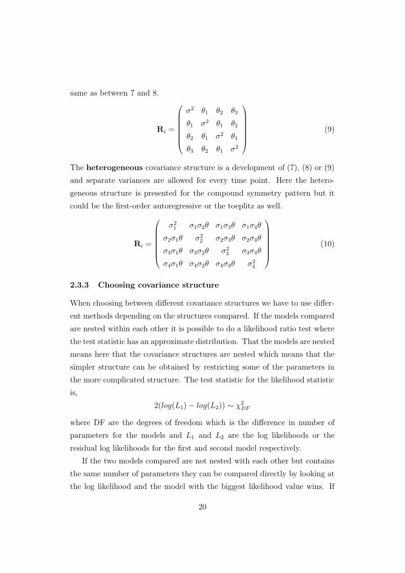
The heterogeneous covariance structure is a development of (7), (8) or (9)

and separate variances are allowed for every time point. Here the hetero-

geneous structure is presented for the compound symmetry pattern but it

could be the first-order autoregressive or the toeplitz as well.

Ri =

σ21 σ1σ2θ σ1σ3θ σ1σ4θ

σ2σ1θ σ22 σ2σ3θ σ2σ4θ

σ3σ1θ σ3σ2θ σ23 σ3σ4θ

σ4σ1θ σ4σ2θ σ4σ3θ σ24

(10)

2.3.3 Choosing covariance structure

When choosing between different covariance structures we have to use differ-

ent methods depending on the structures compared. If the models compared

are nested within each other it is possible to do a likelihood ratio test where

the test statistic has an approximate distribution. That the models are nested

means here that the covariance structures are nested which means that the

simpler structure can be obtained by restricting some of the parameters in

the more complicated structure. The test statistic for the likelihood statistic

is,

2(log(L1) − log(L2)) ∼ χ2DF

where DF are the degrees of freedom which is the difference in number of

parameters for the models and L1 and L2 are the log likelihoods or the

residual log likelihoods for the first and second model respectively.

If the two models compared are not nested with each other but contains

the same number of parameters they can be compared directly by looking at

the log likelihood and the model with the biggest likelihood value wins. If

20

the two models are not nested and contains different number of parameters

the likelihood can not be used directly. The models can then be compared

to a simpler model which is nested within both models and the model that

gives the best improvement is chosen. It is also possible to compare these

models with some of the methods described below.

The bigger the likelihood is the better the model fits data and we use this

when we compare different models but since we are interested in getting as

simple models as possible we also have to consider the number of parameters

in the structures. A model with many parameters usually fits data better

than a model with less number of parameters. It is possible to compute a

so called information criteria and there are different ways to do that and

here we show two of these, Akaikes information criteria (AIC) and Bayesian

information criteria (BIC). The idea with both of these are to punish models

with many parameters in some way. We present the information criteria the

way they are computed in SAS. The AIC value are computed,

AIC = −2LL + 2q

where q is the number of parameters in the covariance structure. Formulated

this way a smaller value of AIC indicates a better model. The BIC value is

computed,

BIC = −2LL + q/(2log(n))

where q is the number of parameters in the covariance structure and n is the

number of effective observations, which means the number of individuals.

Like for AIC a smaller value of BIC is better than a larger.

2.3.4 Choosing fixed effects

When the covariance structure is chosen it is time to look at the fixed ef-

fects and there are different approaches how to choose them. Sometimes

some method like forward, backward or stepwise selection is used to only get

significant effects in the final model. Another approach is to keep all fixed

effects and analyse the result that comes out of that. This latter way is used

21

in clinical trials, like in the example in Chapter 3 where the fixed effects are

specified before the study starts and has to be kept in the model even though

they are not significant.

2.4 Model checking

In our model selection we have accepted the model with the best likelihood

value in relation to the number of parameters but we still do not know if the

model chosen is a good model or even if the normality assumption we have

made is realistic. To check this we look at two types of plots for our data,

normal plots and residual plots to see if the residuals and random effects

seem to follow a normal distribution, if the residuals seem to have a constant

variance and to look for outliers. The predicted values and residuals are

based on y − Xα − Zu.

22

3 A two-period cross-over study with repeated

measurements within the periods

3.1 Description of the study

The data in this example comes from a study where it is investigated what

effect a special drug has on the blood pressure on 47 hypertensive patients

that are already treated with one of the three antihypertensive drugs, beta-

blockers, Ca-antagonists or ACE inhibitors. The main effect of this drug

is not the possible effect on the blood pressure but the drug also contains

antihypertensive substance and can therefore affect the blood pressure as a

side effect and it is of interest to investigate how this drug interacts with

other antihypertensive drugs. The blood pressure is the force that the blood

makes on the arteries and the unit of measurement is mmHg. Measuring

blood pressure gives two values, the higher systolic pressure and the lower

diastolic pressure. The systolic blood pressure is measured when the heart

muscle contracts and the diastolic blood pressure is the pressure when the

heart is at rest.

To be included in the study the patients had to meet some requirements.

The patients had to be over 18 years old, generally healthy with a hyper-

tension that was well controlled with some of the antihypertensive drugs

mentioned above. Women had to be post-menopausal or using some method

of contraception for at least three months before they entered the study.

The drug is compared to a placebo preparation and each patient is treated

in two periods, one with active treatment and one with placebo. This type of

study when each patient is given more than one treatment is called a cross-

over study and is always a repeated measurements study since measurements

are made at least twice on each patient. The time between two treatment

periods are called a wash out period and if the wash out period is not long

enough there is risk to get so called carry-over effects which means that the

effect of the treatment given in one period affects the measurement in coming

23

periods. In our study the wash out period is long enough and we consider the

risk of carry-over effects as very small. The data in our example is repeated in

several ways. In addition to the repeated measurements from the cross-over

study the periods consist of five days each and measurements are taken on

the first and the fifth day and on each of these days eleven measurements are

made on each patient. The first two measurements on each day were made

1 hour and 0.5 hours before the patient were given the treatment. The third

measurement was made right after the treatment was given and after that

measurements were made after 1,2,3,4,6,8 and 12 hours. The patients were

randomized to which treatment to get first and the study is double blind

which means that neither the patient nor the doctor knew in which order

the patients were treated with both treatments. Two of the patients have

missing data, one patient from the group treated with beta-blockers from

whom we only have measurements from the first period on the first day and

one patient among the patients treated with Ca-antagonists who have one

value missing at time point 0 on the second day in the first period. This

should not cause much trouble as we mentioned in section 1.4 when we use

a model with random effects and have as much data as we have.

The question to answer is if there is a difference in blood pressure between

patients who get placebo and patients who get the drug mentioned. To

answer this we need a good model for our data to estimate the difference and

its variance. In this Chapter we analyse these data with help of the theory

in Chapters 1 and 2. We will model diastolic and systolic blood pressures

separately and choose models for both. The first model is for the diastolic

blood pressure and will be called Model 1 and the second model is for the

systolic blood pressure and we call this Model 2.

In Section 3.2 we describe the covariance structure and choose the most

proper one. In Section 3.3 we check the models by doing the plots described

in Section 2.4 and we present the results in Section 3.4 and make conclusions

of this study in Section 3.5.

24

3.2 Choosing model

The aim with this study is to find out whether there is a difference in how

the drug and placebo affects the blood pressure and to test this we need

estimates of the fix effects and the variance components but we do not need

estimates of the random effects. First we describe the covariance structures

that we have tried and then we present the results of these and choose what

structure we shall use for our data. We want to have the possibility to handle

individual and its interactions as a random effect but also be able to structure

the covariances after time point. To do this we have used a mix of two types

of mixed models, the random effects model and the covariance pattern model,

which means that the V matrix is built up by both the G matrix and a R

matrix in which the covariance is partly structured directly. We will find two

models, one for diastolic blood pressure and one for systolic blood pressure.

We use the same fixed effects while we try different covariance structures. We

have not distinguished between patients who get different antihypertensive

drugs but they are treated as one group. The fixed effects will then be

treatment, period, day and time point and the interaction treatment*time.

Since the three factor interaction individual*period*day will be tested we

will also include the interaction term period*day in the fixed effects.

3.2.1 Different covariance structures for the data

The matrix for each person consists of two period blocks with two day blocks

in each and within each day block there are eleven measurements. Since we

do not have any missing data this means that the V matrix for one person

will be of dimension (4∗11)×(4∗11) = 44×44 and the matrix for individual

i will be on the form,

Vi =

11 × 11 11 × 11 11 × 11 11 × 11

11 × 11 11 × 11 11 × 11 11 × 11

11 × 11 11 × 11 11 × 11 11 × 11

11 × 11 11 × 11 11 × 11 11 × 11

(11)

25

There are too many different covariance pattern structures to try them all

and it does not make sense to try too many models. To illustrate how the

structures can be modeled a couple of them are given below. For simplicity

we only use three time points.

In the first structure we have fitted the individual effect as random which

means that we get covariance between all observations within the same pa-

tient. The R matrix is diagonal containing the residuals in this model.

V =

θ θ θ θ θ θ θ θ θ θ θ θ












+ σ2I44 (12)

where the first matrix is ZGZ′ and the second matrix is the R matrix and

where θ is the covariance between measurements made on the same individual

and σ2 is the residual variance.

It is also possible that extra covariance is needed for observations in the

same period and in the next structure we have included the interaction term

26

individual*period.

V =

θp θp θp θp θp θp θ θ θ θ θ θ






θ θ θ θ θ θ θp θp θp θp θp θp






+ σ2I44 (13)

where the first matrix is ZGZ′ and the second matrix is the R matrix

and where θ is the individual covariance and θp is the sum of θ and the

extra covariance for measurements in the same period and σ2 is the residual

variance.

We can also add extra covariance to measurements made at the same day

27

in the periods.

V =

θ1 θ1 θ1 θp θp θp θ2 θ2 θ2 θ θ θ



θp θp θp θ1 θ1 θ1 θ θ θ θ2 θ2 θ2



θ2 θ2 θ2 θ θ θ θ1 θ1 θ1 θp θp θp



θ θ θ θ2 θ2 θ2 θp θp θp θ1 θ1 θ1



+ σ2I44 (14)

where θp is the sum of θ and the covariance for measurements from the same

period, θ1 is the sum of θp the covariance for measurements from the same

day in the periods and θ2 is the sum of θ and the day covariance.

To the previous structure it is possible to add extra covariance for obser-

vations on the same day in the same period. This could be done by adding

the interaction term individual*day*period to the random effects and the

ZGZ′ matrix would then look as in (14) but θ1 would then also include an

extra term which is the three factor interaction. Models where interaction

terms with day is included can partly be modeled in the R matrix. If we for

example include the three factor interaction described we can use different

structures to model the covariance by time point in the R matrix and if the

compound symmetry structure is used to structure the time points the two

ways will be equivalent. In the next example of V we have modeled the

three factor interaction in the R matrix and in this example we have used

the unstructured covariance pattern but it is possible to use that structure

that fits the best. The matrix ZGZ′ looks as in (14) and below we only give

28

the R matrix.

R =

σ2

θ12 θ13 0 0 0 0 0 0 0 0 0

θ12 σ2

θ23 0 0 0 0 0 0 0 0 0

θ13 θ23 σ2 0 0 0 0 0 0 0 0 0

0 0 0 σ2

θ12 θ13 0 0 0 0 0 0

0 0 0 θ12 σ2

θ23 0 0 0 0 0 0

0 0 0 θ13 θ23 σ2 0 0 0 0 0 0

0 0 0 0 0 0 σ2

θ12 θ13 0 0 0

0 0 0 0 0 0 θ12 σ2

θ23 0 0 0

0 0 0 0 0 0 θ13 θ23 σ2 0 0 0

0 0 0 0 0 0 0 0 0 σ2

θ12 θ13

0 0 0 0 0 0 0 0 0 θ12 σ2

θ23

0 0 0 0 0 0 0 0 0 θ13 θ23 σ2

(15)

where θi,j is the covariance between time points i and j and σ2 is the residual

variance.

It is also possible to fit extra covariance for measurements made on the

same time points on the same day or on different days by adding the individ-

ual*time to the random effects. We could also add other interaction terms

with individual and time to the model. We will not try any of these models

for our data and therefore we do not describe them further. If there had been

more periods or days the covariance pattern could have been structured by

them in the same way that it is structured by the time points. Since there

are only two periods and two days it does not make sense to use them to

structure the covariance.

3.2.2 Choosing covariance structure

When we choose a model we start with a simple model and go on with more

and more complicated models. As we discussed above we have many mea-

29

surements on every individual and the V matrix could be complicated and

the estimation process very demanding if we use too complicated structures

on the time points. Therefore we will not have time to try for example the

unstructured covariance structure which is a saturated model in the sense

that the blocks in the R matrix would then be saturated and should give the

best likelihood value but it is not very likely that this model would be the

best because of the large number of parameters. We will now list all models

we tried and their -2RLL measures and their AIC values. After that we give

a discussion of which model is the best for our data. SAS gives us a calcula-

tion of -2 residual log likelihood which is denoted -2RLL. To choose among

the different covariance structures above we use the methods described in

Section 2.3.3.

Covariance structure for Model 1

We start with the model for diastolic blood pressure. In the table below ind

means individual, per means period and when R has a structure other than

diagonal it follows the structure in (15). When models are compared with

likelihood ratio tests the more complicated model are chosen if the hypothesis

of ’no improvement of the likelihood with respect to the difference in number

of parameters’ can be rejected on a 5% level. Model A1 and B1 are nested

and we compare them with a likelihood ratio test where the test statistic

is 12191.6-12061.7=129.9 which is χ2-distributed with 1 degree of freedom

and gives a p-value very close to 0. Also models B1 and C1 are nested

and comparison of these gives a test statistic of 12061.7-12037.3=24.4 with 1

degree of freedom. The p-value for this is near 0 and we reject the hypothesis

and choose model C1 over B1. In model D1 we have added the three factor

interaction between individual, period and day. Testing D1 against C1 gives

a test statistic 12037.3-11927.3=110 with 1 degree of freedom which will give

a p-value near 0 which means that model D1 is preferable. For model D1 the

G matrix will not be positive definite and it turns out that the random effect

individual*period has been estimated to be negative and SAS therefore sets

30

Model Random effects R struc. Param. -2RLL AIC

A1 ind diag. 2 12191.6 12195.6

B1 ind, ind*per diag. 3 12061.7 12067.7

C1 ind, ind*per, ind*day diag. 4 12037.3 12045.3

D1 ind*per*day and lower diag. 5 11927.3 11937.3

E1 ind, ind*per cs 4 11927.3 11935.3

F1 ind, ind*per csh 14 11915.0 11943.0

G1 ind, ind*per ar(1) 4 11729.9 11737.9

H1 ind, ind*per arh(1) 14 11712.1 11740.1

I1 ind, ind*per toep 13 11704.0 11730.0

J1 ind, ind*per toeph 23 16183.5 16225.5

K1 ind, ind*per/tr toep/tr 26 11752.8* 11802.8*

*Hessian matrix not positive definite

Table 1: Models tried for the diastolic blood pressure

it to 0 as described in Section 1.3.4. This means that the interaction between

individual and day we seemed to find in model C1 was significant because

we need an extra covariance for measurements made on the same individual

on the same day but also in the same period. That the model will be the

same without individual*day is illustrated by the next model F1 which is

the same model as D1 but without individual*day and with the difference

that the three factor interaction is modeled in the R matrix. The way E1

is parametrised, like in (7), it is not nested within F1, parametrised like in

(10) which means they can be compared with a likelihood ratio test. The

improvement from model E1 to model F1 is rather big, 11927.3-11915.0=12.2

but the difference in number of parameters is large, 14-4=10 which makes

the AIC value for model E1 better than for model F1. Models E1 and G1

are not nested but contains the same number of parameters which makes

it possible to compare the likelihoods directly and since G1 has a better

value on -2RLL we will choose that over model E1. Models H1 and G1 are

31

nested and the χ2-statistic in the comparison between these models will be

11729.9-11712.1=17.8 with 10 degrees of freedom which gives the p-value

0.0584 which is almost significant but we choose model G1. In model I1

we have the toeplitz pattern which is also called the general autoregressive

model which means that we can get the autoregressive structure by restricting

parameters in the toeplitz structure so they are nested. The test statistic will

be 11729.9-11704.0=25.9 with 9 degrees of freedom and the p-value for this

test will be 0.0021 and we can reject the hypothesis of no improvement and

we choose the toeplitz structure over the autoregressive. Model J1 has a value

of -2RLL that is much higher than the other models which is not reasonable

and unfortunately we do not have time to investigate this further. It seems

that model G1 has the best structure of all tried to fit these data and in

the last model we investigate if we need different values of the covariance

parameters for the two treatments like in model I1. It should be reasonable

to think that the variation between individuals should increase when they

are given active treatment since people respond differently to a treatment.

Model I1 has a value of -2RLL that is higher than model G2 which should be

impossible since the models are nested. The reason to this is that the Hessian

matrix in the estimation process is not positive definite which means that the

determinant is negative and at least one of the second derivatives is negative

and the value of -2RLL grows in some direction. In SAS PROC MIXED it

is possible to choose starting point but due to time limitations we can not

investigate this model further. For our analysis of diastolic blood pressure

we choose model I1 with individual and individual*period as random and a

toeplitz pattern on the time points in the same period on the same day which

means that we have different covariances for every level of separation in time

points.

Covariance structre for Model 2

Now we will decide which model to use for systolic blood pressure data and we

start by giving a table with the models and their goodness-of-fit measures.

32

Model Random effects R struc. Param. -2RLL AIC

A2 ind diag. 2 14053.9 14057.9

B2 ind, ind*per diag. 3 13930.8 13936.8

C2 ind, ind*per, ind*day diag. 4 13919.8 13927.8

D2 ind*per*day and lower diag. 5 13816.7 13824.7

E2 ind, ind*per cs 4 13816.7 13824.7

F2 ind, ind*per csh 14 13757.5 13785.5

G2 ind, ind*per ar(1) 4 13571.8 13579.8

H2 ind, ind*per arh(1) 14 13514.9 13542.9

I2 ind, ind*per toep 13 13517.9 13543.9

J2 ind, ind*per toeph 23 27742.0 27784.0

K2 ind, ind*per/gr toep/gr 26 13578.1* 13630.1*

*Hessian matrix is not positive definite

Table 2: Models tried for the diastolic blood pressure

We have tried the same models as for the diastolic data. Models A2 and

B2 are nested and the difference in -2RLL which is 14053.9-13930.8=123.1

which is χ2-distributed with 3-2=1 degree of freedom and gives a p-value

very close to 0. We choose B2 over A2 and go on with comparing model B2

with model C2. These two are also nested and the difference in -2RLL is

13930.8-13919.5=11 and the degrees of freedom is 1. This gives a p-value of

0.0009 and we choose model C2 over B2. Model D2 gives an improvement

from C2 of the -2RLL value of 103 and since the difference in degrees of

freedom is only 1 the p-value will again be very close to 0 and we prefer

model D2 of these two. As for Model 1 the interaction term individual*day

is estimated to be negative and set to 0 and gives the same result as in

the next model E2. E2 and F2 are not nested but since model G2 has lower

value of -2RLL than both E2 and F2 and as many parameters as E2 and fewer

parameters than F2 we can choose G2 over both E2 and F2. In model H2 we

have different variances for every time point and G2 is nested within H2 and

33

comparing these models gives the test statistic 13571.8-13514.9=56.9 with

10 degrees of freedom which gives a p-value near 0 which says that model

H2 is better than model G2. The toeplitz structure is nested within the

heterogeneous autoregressive structure and the difference in -2LL is 13517.9-

13514.9=3 which has 1 degree of freedom. The p-value for this is 0.0833

which means that the difference is not significant and we choose the model

with fewer parameters which is the toeplitz pattern in model I2. Like in

Model 1 the model with the heterogeneous toeplitz pattern does not behave

as expected and the value of -2RLL is more than twice as high as in model

I2. We therefore choose the toeplitz pattern as our covariance structure in

the R matrix. We also try to fit different values of the covariance parameter

for different treatments but as for Model 1 the Hessian matrix is not positive

definite and the value of -2RLL is higher than in model I2 so we can not make

any conclusions about which model is the best. As for Model 1 we choose the

toeplitz pattern in the R matrix and it seems reasonable to use same model

for both diastolic and systolic blood pressure since they will probably follow

each other.

3.2.3 Choosing fixed effects

In Section 2.3.4 we discussed how to choose fixed effects and since this is

a clinical study the fixed effects were chosen before the study started and

we have to keep all fixed effects in the model even though they are not all

significant as we will see in Section 3.4.

3.3 Model checking

We check the normality assumption and how well data fits our models with

residual plots and normal quantile plots both described in Chapter 2.4.

34

Figure 1: Residual plot for the model for diastolic blood pressure

Figure 2: Normal plot for the model for diastolic blood pressure

35

Model 1

By looking at the residual plot in figure 1 we can see that the residuals seems

to be randomly distributed with constant variance. We have one rather big

outlier with the predicted value 74.5 but since the total number of observa-

tions is large it should not affect the results. Figure 2 is a normal plot and it

shows that our assumption about normality seems to be correct. The about

20 measurements that diverge in the beginning and the end of the line is

not a problem for our assumption since the rest of the measurements are so

many and follow the line almost perfectly.

Model 2

In the residual plot in Figure 3 we can see that the dispersion of the systolic

blood pressure is bigger than for the diastolic blood pressure but it still seems

like the residuals are randomly distributed with constant variance. Why the

dispersion is bigger for the systolic blood pressure than for the diastolic and

if this is reasonable cannot be answered by a statistician but by a doctor

or someone else with knowledge about the heart and human body. The

normal plot in Figure 4 does not follow the straight line as well as for the

diastolic blood pressure but still well enough for us to accept the normality

assumption.

36

Figure 3: Residual plot for the model for systolic blood pressure.

Figure 4: Normal plot for the model for systolic blood pressure.

37

Effect Num DF Den DF F-value Pr> F

Period 1 44.1 0.38 0.5432

Day 1 90.2 0.00 0.9898

Treatment 1 44.5 13.46 0.0006

Time 10 737 191.58 <0.0001

Treatment*Time 10 737 13.92 <0.0001

Period*Day 1 90.2 0.55 0.4602

Table 3: Tests for the fixed effects in the model for diastolic blood pressure

3.4 Results

We want to estimate the differences between the two treatments and to begin

with we first look at the fixed effects to see if treatment is a significant factor

at all. The fixed effects will be tested with the Wald statistic described in

Section 1.3.5 where the denominator degrees of freedom is calculated with

Kenward Rogers method. If the treatment effect is significant we go on with

looking at the differences of the least squares estimates for the two treatments

and we investigate if the difference is significant.

Results from Model 1

Below we give a table with tests of the fixed effects.

As we can see in Table 3 both the treatment effect and the interaction

effect between treatment and time are significant. This means that there

are differences between the treatments and we go on with looking closer

at the estimates. Since the interaction effect is also significant it will not

be appropriate to compare the over all effects but we have to compare the

treatment effects at each time point we are interested in. None of the effects

period, day or period*day are significant which is good. We do not want

the drugs to act different at differently occasions. Before we look at the

differences in treatment effect we look at the estimates of the covariance

parameters which are used in the estimations of the standard errors. We

38

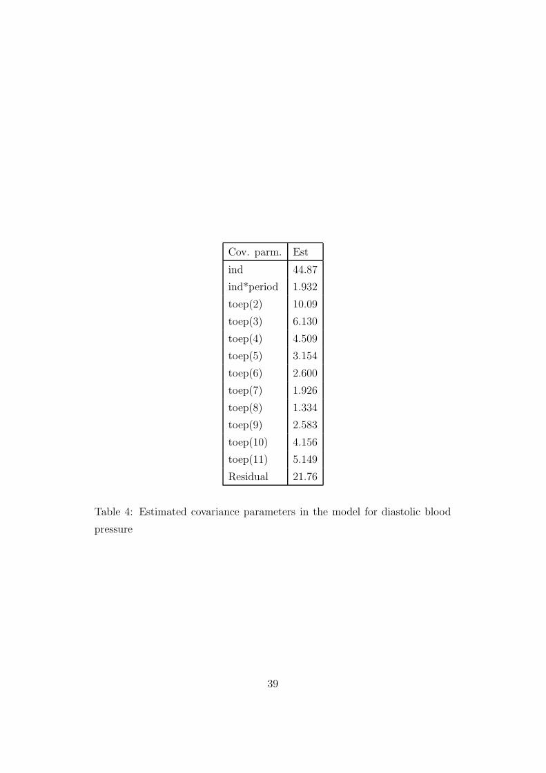
Cov. parm. Est

ind 44.87

ind*period 1.932

toep(2) 10.09

toep(3) 6.130

toep(4) 4.509

toep(5) 3.154

toep(6) 2.600

toep(7) 1.926

toep(8) 1.334

toep(9) 2.583

toep(10) 4.156

toep(11) 5.149

Residual 21.76

Table 4: Estimated covariance parameters in the model for diastolic blood

pressure

39

expected that measurements closer in time have higher correlation than those

with a higher level of separation which seems to be true for lower levels of

separation but not for the three highest. When we see these estimates of

the toeplitz parameters it is easy to understand why the toeplitz pattern

is the best choice of the structures on R that we tried. None of the other

models allow for higher correlations between time points with high level of

separation than time points with low level of separation. We can not find an

explanation for this yet but we have to see more of the results. Now we can

estimate the standard errors and below we give a table with the standard

errors, the least squares means of the treatment effects for both treatments

and the interaction effects between treatment and time for both treatments

and every time point. The time is given in hours and time point 0 is when

the patient is given the drug. We plot the estimates when given the active

drug and the estimates given the placebo in the same picture against time

to see how the blood pressure vary with time and to get a picture of the

difference between the active drug and placebo. In Figure 5 we can see that

for both treatments the blood pressure is higher in the beginning and in the

end and lower in the middle with a smaller increase 4 hours after taken the

drug. That the pressure goes down in the beginning and increases in the end

can either be an effect of that the patients are given a drug, active or placebo,

or that the blood pressure varies naturally. Since we have the same increase

for both treatments after four hour we can believe that something always

happened on this time point, like that the patients were given something to

eat. In Figure 5 we probably have an explanation to the unexpected values

on the toeplitz parameters. Since the blood pressures for both treatments

go back to the values where they started the correlation between the first

and the last time points will at least look more correlated than time points

with a lower level of separation. We want to see if the difference is significant

for any of the time points and in the table below we have calculated the

differences for every time point, their standard errors based on the pooled

variance, the degrees of freedom, t-values and p-values. The difference is

40

Effect Treatm. Time Est. SE DF t-value Pr> |t|

treat active 73.29 1.109 51.6 71.30 <0.0001

treat placebo 75.02 1.109 51.9 72.83 <0.0001

treat*time active -1 79.99 1.109 68.7 72.76 <0.0001

treat*time active -0.5 79.98 1.109 68.7 72.41 <0.0001

treat*time active 0 80.36 1.109 68.7 72.76 <0.0001

treat*time active 0.5 80.37 1.109 68.7 72.76 <0.0001








treat*time placebo -1 78.88 1.112 69.3 71.23 <0.0001

treat*time placebo -0.5 79.44 1.112 69.3 71.74 <0.0001

treat*time placebo 0 79.39 1.113 69.5 71.64 <0.0001

treat*time placebo 0.5 74.13 1.112 69.3 66.94 <0.0001








Table 5: Estimates of the treatmenteffects for the diastolic blood pressure

41

−2 0 2 4 6 8 10 1264

66

68

70

72

74

76

78

80

82Diastolic bp

Time

Blo

od p

ress

ure

activeplacebo

Figure 5: Estimates of the diastolic blood pressure for the active treatment

and the placebo.

calculated as the estimate of the active drug minus the estimate of placebo.

We reject the hypothesis of ’no difference’ if the p-value is lower than 5%

and the test is two sided. As expected we do not seem to have any difference

in treatment effect for the first three time points and neither for the first

time point after the drug is given. Half an hour later we have a difference

that is significant and after that we have highly significant differences until

somewhere between 6 and 8 hours after the drug is given and after that

we do not have any significant differences. It seems like the effect on the

diastolic blood pressure of the active drug starts somewhere between 0.5 and

1 hours and stops somewhere between 6 and 8 hours after the drug is taken.

Since the estimates of the significant differences are negative we can make the

conclusion that the active drug gives lower blood pressure than the placebo.

42

Time Est SE DF t-value Pr> |t|

-1 1.111 0.7533 259 1.49 0.1372

-0.5 0.5357 0.7533 259 0.72 0.4728

0 0.9776 0.7546 259 1.31 0.1913

0.5 0.1905 0.7533 259 0.26 0.7984

1 -1.550 0.7533 259 -2.08 0.0385

2 -5.165 0.7533 259 -6.93 <0.0001

3 -6.573 0.7533 259 -8.82 <0.0001

4 -6.084 0.7533 259 -8.17 <0.0001

6 -2.718 0.7533 259 -3.65 0.0003

8 -0.2108 0.7533 259 -0.28 0.7775

12 0.4512 0.7533 259 0.61 0.5453

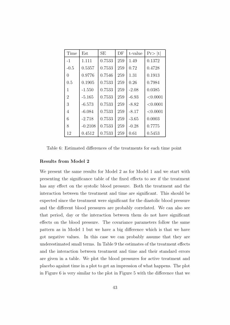
Table 6: Estimated differences of the treatments for each time point

Results from Model 2

We present the same results for Model 2 as for Model 1 and we start with

presenting the significance table of the fixed effects to see if the treatment

has any effect on the systolic blood pressure. Both the treatment and the

interaction between the treatment and time are significant. This should be

expected since the treatment were significant for the diastolic blood pressure

and the different blood pressures are probably correlated. We can also see

that period, day or the interaction between them do not have significant

effects on the blood pressure. The covariance parameters follow the same

pattern as in Model 1 but we have a big difference which is that we have

got negative values. In this case we can probably assume that they are

underestimated small terms. In Table 9 the estimates of the treatment effects

and the interaction between treatment and time and their standard errors

are given in a table. We plot the blood pressures for active treatment and

placebo against time in a plot to get an impression of what happens. The plot

in Figure 6 is very similar to the plot in Figure 5 with the difference that we

43

Effect Num DF Den DF F-value Pr>F

Period 1 44.1 1.51 0.2256

Day 1 89.8 0.01 0.9166

Treatment 1 45 7.02 0.0111

Time 10 743 132.28 <0.0001

Treatment*time 10 743 12.05 <0.0001

Period*Day 1 89.8 0.77 0.3817

Table 7: Tests for the fixed effects in the model for systolic blood pressure

Cov. parm. Est

ind 122.2

ind*per 5.117

toep(2) 26.78

toep(3) 15.62

toep(4) 13.19

toep(5) 8.772

toep(6) 4.054

toep(7) -1.033

toep(8) -0.4705

toep(9) 0.3753

toep(10) 10.06

toep(11) 12.44

Residual 55.29

Table 8: Estimated covariance parameters in the model for the systolic blood

pressure

44

Effect Treatm. Time Est. SE DF t-value Pr> |t|

treat active 128.9 1.697 50.6 75.96 <0.0001

treat placebo 130.9 1.700 50.9 76.98 <0.0001

treat*time active -1 137.3 1.818 66.6 75.52 <0.0001

treat*time active -0.5 137.6 1.818 66.6 75.65 <0.0001


treat*time active 0.5 131.6 1.818 66.6 72.37 <0.0001








treat*time placebo -1 134.9 1.822 67.1 74.02 <0.0001

treat*time placebo -0.5 135.4 1.822 67.1 74.28 <0.0001


treat*time placebo 0.5 131.5 1.822 67.1 72.15 <0.0001








Table 9: Estimates of the treatmenteffects for the systolic blood pressure

45

−2 0 2 4 6 8 10 12115

120

125

130

135

140

145Systolic bp

Time

Blo

od p

ress

ure

activeplacebo

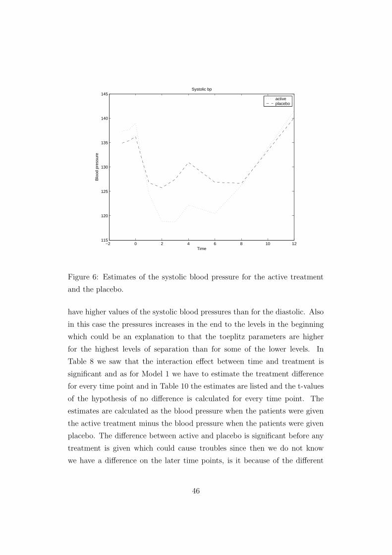
Figure 6: Estimates of the systolic blood pressure for the active treatment

and the placebo.

have higher values of the systolic blood pressures than for the diastolic. Also

in this case the pressures increases in the end to the levels in the beginning

which could be an explanation to that the toeplitz parameters are higher

for the highest levels of separation than for some of the lower levels. In

Table 8 we saw that the interaction effect between time and treatment is

significant and as for Model 1 we have to estimate the treatment difference

for every time point and in Table 10 the estimates are listed and the t-values

of the hypothesis of no difference is calculated for every time point. The

estimates are calculated as the blood pressure when the patients were given

the active treatment minus the blood pressure when the patients were given

placebo. The difference between active and placebo is significant before any

treatment is given which could cause troubles since then we do not know

we have a difference on the later time points, is it because of the different

46

Time Est SE DF t-value Pr> |t|

-1 2.414 1.1937 264 2.02 0.0444

-0.5 2.175 1.1937 264 1.82 0.0699

0 2.819 1.1958 266 2.33 0.0204

0.5 0.07873 1.1937 264 0.06 0.9493

1 -2.2434 1.1937 264 -1.88 0.0610

2 -6.865 1.1937 264 -5.75 <0.0001

3 -8.841 1.1937 264 -7.41 <0.0001

4 -8.691 1.1937 264 -7.28 <0.0001

6 -3.519 1.1937 264 -2.95 0.0035

8 -0.5535 1.1937 264 -0.47 0.6416

12 1.417 1.1937 264 1.18 0.2373

Table 10: Estimated differences of the treatments for each time point

treatments or is it because the levels are different from the beginning. We

can see that the estimate of the difference changes signs from positive to

negative after 1 hour and then stays negative until the last time point. This

means that we can make conclusions about the significant differences.

3.5 Conclusions

Our two models gives similar results. It seems like the diastolic and the

systolic blood pressure react in the same way to the treatments. From our

models we can draw the conclusions that the active drug does affect the

blood pressure. The effect seems to come after about 1 hour after the drug

is taken and stops working after about 8 hours. The answer to our question

in the beginning of this Chapter is that the drug investigated does affect the

blood pressure for persons who are treated with antihypertensive drugs in

the way that the pressure decreases. Since the wanted effect of the drug is

not to decrease the blood pressure this will maybe be a problem. To make

conclusions about if this drug should be given to hypertensive patients treated

47

with antihypertensive drugs a doctor should be consulted. The doctor knows

if the decrease in blood pressure is too big and if it is worth the positive effect

of the drug.

48

References

[1] Helen Brown and Robin Prescott, Applied mixed models in medicine,

Wiley cop. 1999.

[2] Charles S. Davis, Statistical methods for the analysis of repeated mea-

surements, Springer-Verlag New York, Inc 2002

[3] Peter J. Diggle, Kung-Yee Liang and Scott L.Zegar, Analysis of longi-

tudinal data, Oxford Science publications 1996.

[4] Charles E. McCulloch, Shayle R. Searle, Generalized, linear and mixed

models, John Wiley & Sons, Inc 2001.

[5] David Hand and Martin Crowder, Practical longitudinal data analysis,

Chapman & Hall 1996.

[6] Michael G. Kenward and James H. Roger, Small sample inference for

fixed effects from resticted maximum likelihood, Biometrics. Vol 53, No.3

(Sep., 1997) 983-997

49

Documents

Using mixed models in a cross-over study with repeated ... · Mathematical Statistics Stockholm University Using mixed models in a cross-over study with repeated measurements within