��������

��� �������� �� ����������

�������

Edward NeumanDepartment of Mathematics

Southern Illinois University at Carbondaleedneuman@siu.edu

One of the nice features of MATLAB is its ease of computations with vectors and matrices. Inthis tutorial the following topics are discussed: vectors and matrices in MATLAB, solvingsystems of linear equations, the inverse of a matrix, determinants, vectors in n-dimensionalEuclidean space, linear transformations, real vector spaces and the matrix eigenvalue problem.Applications of linear algebra to the curve fitting, message coding and computer graphics are alsoincluded.

�� ������������������ ��������� ���� ������ ��������

For the reader's convenience we include lists of special characters and MATLAB functions thatare used in this tutorial.

Special characters; Semicolon operator' Conjugated transpose.' Transpose* Times. Dot operator^ Power operator[ ] Emty vector operator: Colon operator= Assignment

== Equality\ Backslash or left division/ Right division

i, j Imaginary unit~ Logical not

~= Logical not equal& Logical and| Logical or

{ } Cell

2

Function Descriptionacos Inverse cosineaxis Control axis scaling and appearancechar Create character arraychol Cholesky factorizationcos Cosine function

cross Vector cross productdet Determinantdiag Diagonal matrices and diagonals of a matrix

double Convert to double precisioneig Eigenvalues and eigenvectorseye Identity matrixfill Filled 2-D polygonsfix Round towards zero

fliplr Flip matrix in left/right directionflops Floating point operation countgrid Grid lines

hadamard Hadamard matrixhilb Hilbert matrixhold Hold current graphinv Matrix inverse

isempty True for empty matrixlegend Graph legendlength Length of vector

linspace Linearly spaced vectorlogical Convert numerical values to logicalmagic Magic squaremax Largest componentmin Smallest component

norm Matrix or vector normnull Null space

num2cell Convert numeric array into cell arraynum2str Convert number to string

ones Ones arraypascal Pascal matrixplot Linear plotpoly Convert roots to polynomial

polyval Evaluate polynomialrand Uniformly distributed random numbers

randn Normally distributed random numbersrank Matrix rankreff Reduced row echelon formrem Remainder after division

reshape Change sizeroots Find polynomial rootssin Sine functionsize Size of matrixsort Sort in ascending order

3

subs Symbolic substitutionsym Construct symbolic bumbers and variablestic Start a stopwatch timer

title Graph titletoc Read the stopwatch timer

toeplitz Tioeplitz matrixtril Extract lower triangular parttriu Extract upper triangular part

vander Vandermonde matrixvarargin Variable length input argument list

zeros Zeros array

���������� ���������� ������

The purpose of this section is to demonstrate how to create and transform vectors and matrices inMATLAB.

This command creates a row vector

a = [1 2 3]

a = 1 2 3

Column vectors are inputted in a similar way, however, semicolons must separate the componentsof a vector

b = [1;2;3]

b = 1 2 3

The quote operator ' is used to create the conjugate transpose of a vector (matrix) while the dot-quote operator .' creates the transpose vector (matrix). To illustrate this let us form a complexvector a + i*b' and next apply these operations to the resulting vector to obtain

(a+i*b')'

ans = 1.0000 - 1.0000i 2.0000 - 2.0000i 3.0000 - 3.0000i

while

4

(a+i*b').'

ans = 1.0000 + 1.0000i 2.0000 + 2.0000i 3.0000 + 3.0000i

Command length returns the number of components of a vector

length(a)

ans = 3

The dot operator. plays a specific role in MATLAB. It is used for the componentwise applicationof the operator that follows the dot operator

a.*a

ans = 1 4 9

The same result is obtained by applying the power operator ^ to the vector a

a.^2

ans = 1 4 9

Componentwise division of vectors a and b can be accomplished by using the backslash operator\ together with the dot operator .

a.\b'

ans = 1 1 1

For the purpose of the next example let us change vector a to the column vector

a = a'

a = 1 2 3

The dot product and the outer product of vectors a and b are calculated as follows

dotprod = a'*b

5

dotprod = 14 outprod = a*b'

outprod = 1 2 3 2 4 6 3 6 9

The cross product of two three-dimensional vectors is calculated using command cross. Let thevector a be the same as above and let

b = [-2 1 2];

Note that the semicolon after a command avoids display of the result. The cross product of a andb is

cp = cross(a,b)

cp = 1 -8 5

The cross product vector cp is perpendicular to both a and b

[cp*a cp*b']

ans = 0 0

We will now deal with operations on matrices. Addition, subtraction, and scalar multiplication aredefined in the same way as for the vectors.

This creates a 3-by-3 matrix

A = [1 2 3;4 5 6;7 8 10]

A = 1 2 3 4 5 6 7 8 10

Note that the semicolon operator ; separates the rows. To extract a submatrix B consisting ofrows 1 and 3 and columns 1 and 2 of the matrix A do the following

B = A([1 3], [1 2])

B = 1 2 7 8

To interchange rows 1 and 3 of A use the vector of row indices together with the colon operator

C = A([3 2 1],:)

6

C = 7 8 10 4 5 6 1 2 3

The colon operator : stands for all columns or all rows. For the matrix A from the last examplethe following command

A(:)

ans = 1 4 7 2 5 8 3 6 10

creates a vector version of the matrix A. We will use this operator on several occasions.

To delete a row (column) use the empty vector operator [ ]

A(:, 2) = []

A = 1 3 4 6 7 10

Second column of the matrix A is now deleted. To insert a row (column) we use the technique forcreating matrices and vectors

A = [A(:,1) [2 5 8]' A(:,2)]A = 1 2 3 4 5 6 7 8 10

Matrix A is now restored to its original form.

Using MATLAB commands one can easily extract those entries of a matrix that satisfy an impsedcondition. Suppose that one wants to extract all entries of that are greater than one. First, wedefine a new matrix A

A = [-1 2 3;0 5 1]

A = -1 2 3 0 5 1

7

Command A > 1 creates a matrix of zeros and ones

A > 1

ans = 0 1 1 0 1 0

with ones on these positions where the entries of A satisfy the imposed condition and zeroseverywhere else. This illustrates logical addressing in MATLAB. To extract those entries of thematrix A that are greater than one we execute the following command

A(A > 1)

ans = 2 5 3

The dot operator . works for matrices too. Let now

A = [1 2 3; 3 2 1] ;

The following command

A.*A

ans = 1 4 9 9 4 1

computes the entry-by-entry product of A with A. However, the following command

A*A

¨??? Error using ==> *Inner matrix dimensions must agree.

generates an error message.

Function diag will be used on several occasions. This creates a diagonal matrix with the diagonalentries stored in the vector d

d = [1 2 3];

D = diag(d)

D = 1 0 0 0 2 0 0 0 3

8

To extract the main diagonal of the matrix D we use function diag again to obtain

d = diag(D)

d = 1 2 3

What is the result of executing of the following command?

diag(diag(d));

In some problems that arise in linear algebra one needs to calculate a linear combination ofseveral matrices of the same dimension. In order to obtain the desired combination both thecoefficients and the matrices must be stored in cells. In MATLAB a cell is inputted using curlybraces{ } . This

c = {1,-2,3}

c = [1] [-2] [3]

is an example of the cell. Function lincomb will be used later on in this tutorial.

function M = lincomb(v,A)

% Linear combination M of several matrices of the same size.% Coefficients v = {v1,v2,…,vm} of the linear combination and the% matrices A = {A1,A2,...,Am} must be inputted as cells.

m = length(v);[k, l] = size(A{1});M = zeros(k, l);for i = 1:m M = M + v{i}*A{i};end

���� � ��!��������� ����"����� �

MATLAB has several tool needed for computing a solution of the system of linear equations.

Let A be an m-by-n matrix and let b be an m-dimensional (column) vector. To solvethe linear system Ax = b one can use the backslash operator \ , which is also called the leftdivision.

9

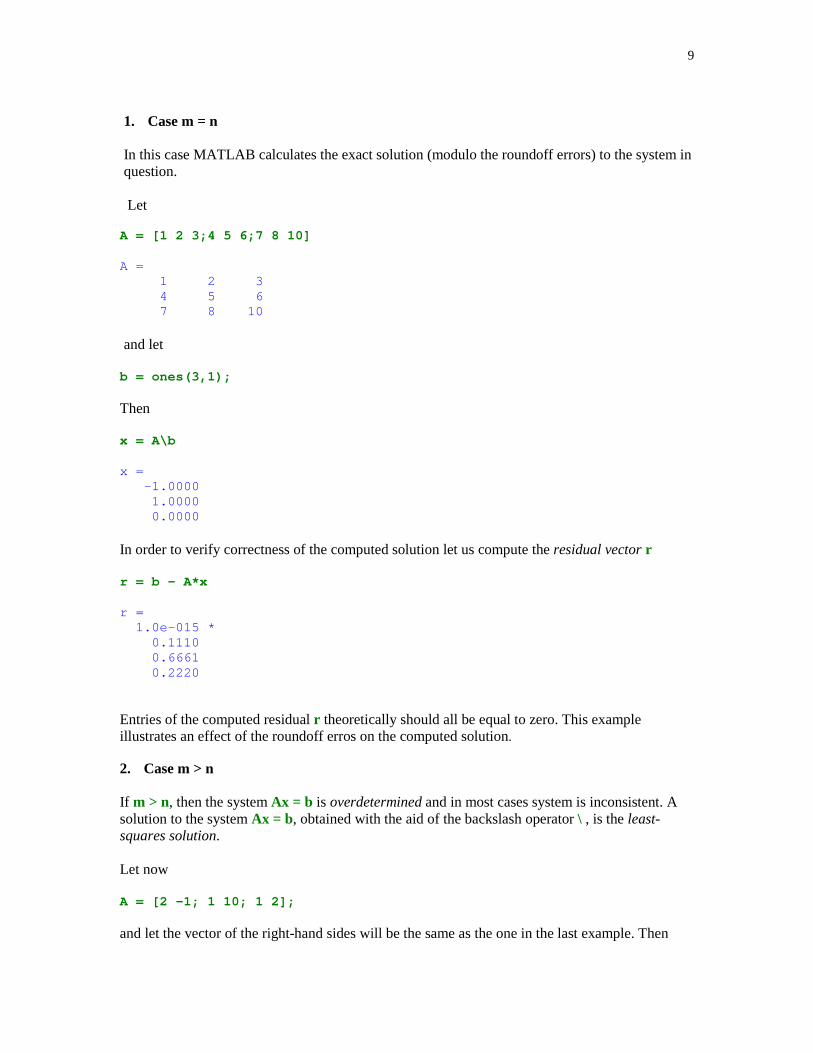
1. Case m = n

In this case MATLAB calculates the exact solution (modulo the roundoff errors) to the system inquestion.

Let

A = [1 2 3;4 5 6;7 8 10]

A = 1 2 3 4 5 6 7 8 10

and let

b = ones(3,1);

Then

x = A\b

x = -1.0000 1.0000 0.0000

In order to verify correctness of the computed solution let us compute the residual vector r

r = b - A*x

r = 1.0e-015 * 0.1110 0.6661 0.2220

Entries of the computed residual r theoretically should all be equal to zero. This exampleillustrates an effect of the roundoff erros on the computed solution.

2. Case m > n

If m > n, then the system Ax = b is overdetermined and in most cases system is inconsistent. Asolution to the system Ax = b, obtained with the aid of the backslash operator \ , is the least-squares solution.

Let now

A = [2 –1; 1 10; 1 2];

and let the vector of the right-hand sides will be the same as the one in the last example. Then

10

x = A\bx = 0.5849 0.0491

The residual r of the computed solution is equal to

r = b - A*x

r = -0.1208 -0.0755 0.3170

Theoretically the residual r is orthogonal to the column space of A. We have

r'*A

ans = 1.0e-014 * 0.1110 0.6994

3. Case m < n

If the number of unknowns exceeds the number of equations, then the linear system isunderdetermined. In this case MATLAB computes a particular solution provided the system isconsistent. Let now

A = [1 2 3; 4 5 6];b = ones(2,1);

Then

x = A\b

x = -0.5000 0 0.5000

A general solution to the given system is obtained by forming a linear combination of x with thecolumns of the null space of A. The latter is computed using MATLAB function null

z = null(A)

z = 0.4082 -0.8165 0.4082

11

Suppose that one wants to compute a solution being a linear combination of x and z, withcoefficients 1 and –1. Using function lincomb we obtainw = lincomb({1,-1},{x,z})

w = -0.9082 0.8165 0.0918

The residual r is calculated in a usual way

r = b - A*w

r = 1.0e-015 * -0.4441 0.1110

�#$� ���� ����� �������������� �

The built-in function rref allows a user to solve several problems of linear algebra. In this sectionwe shall employ this function to compute a solution to the system of linear equations and also tofind the rank of a matrix. Other applications are discussed in the subsequent sections of thistutorial.

Function rref takes a matrix and returns the reduced row echelon form of its argument. Syntax ofthe rref command is

B = rref(A) or [B, pivot] = rref(A)

The second output parameter pivot holds the indices of the pivot columns.

Let

A = magic(3); b = ones(3,1);

A solution x to the linear system Ax = b is obtained in two steps. First the augmented matrix ofthe system is transformed to the reduced echelon form and next its last column is extracted

[x, pivot] = rref([A b])

x = 1.0000 0 0 0.0667 0 1.0000 0 0.0667 0 0 1.0000 0.0667pivot = 1 2 3

12

x = x(:,4)

x = 0.0667 0.0667 0.0667

The residual of the computed solution is

b - A*x

ans = 0 0 0

Information stored in the output parameter pivot can be used to compute the rank of the matrix A

length(pivot)

ans = 3

�%���� ������������&

MATLAB function inv is used to compute the inverse matrix.

Let the matrix A be defined as follows

A = [1 2 3;4 5 6;7 8 10]

A = 1 2 3 4 5 6 7 8 10

Then

B = inv(A)

B = -0.6667 -1.3333 1.0000 -0.6667 3.6667 -2.0000 1.0000 -2.0000 1.0000

In order to verify that B is the inverse matrix of A it sufficies to show that A*B = I andB*A = I , where I is the 3-by-3 identity matrix. We have

13

A*B

ans = 1.0000 0 -0.0000 0 1.0000 0 0 0 1.0000

In a similar way one can check that B*A = I .

The Pascal matrix, named in MATLAB pascal, has several interesting properties. Let

A = pascal(3)

A = 1 1 1 1 2 3 1 3 6

Its inverse B

B = inv(A)

B = 3 -3 1 -3 5 -2 1 -2 1

is the matrix of integers. The Cholesky triangle of the matrix A is

S = chol(A)

S = 1 1 1 0 1 2 0 0 1

Note that the upper triangular part of S holds the binomial coefficients. One can verify easily thatA = S'*S.

Function rref can also be used to compute the inverse matrix. Let A is the same as above. Wecreate first the augmented matrix B with A being followed by the identity matrix of the same sizeas A. Running function rref on the augmented matrix and next extracting columns four throughsix of the resulting matrix, we obtain

B = rref([A eye(size(A))]);

B = B(:, 4:6)

B = 3 -3 1 -3 5 -2 1 -2 1

14

To verify this result, we compute first the product A *B

A*B

ans = 1 0 0 0 1 0 0 0 1

and next B*A

B*A

ans = 1 0 0 0 1 0 0 0 1

This shows that B is indeed the inverse matrix of A.

�' (������ � ��

In some applications of linear algebra knowledge of the determinant of a matrix is required.MATLAB built-in function det is designed for computing determinants.

Let

A = magic(3);

Determinant of A is equal to

det(A)

ans = -360

One of the classical methods for computing determinants utilizes a cofactor expansion. For moredetails, see e.g., [2], pp. 103-114.

Function ckl = cofact(A, k, l) computes the cofactor ckl of the akl entry of the matrix A

function ckl = cofact(A,k,l)

% Cofactor ckl of the a_kl entry of the matrix A.

[m,n] = size(A);if m ~= n error( 'Matrix must be square' )

15

endB = A([1:k-1,k+1:n],[1:l-1,l+1:n]);ckl = (-1)^(k+l)*det(B);

Function d = mydet(A) implements the method of cofactor expansion for computingdeterminants

function d = mydet(A)

% Determinant d of the matrix A. Function cofact must be% in MATLAB's search path.

[m,n] = size(A);if m ~= n error( 'Matrix must be square' )enda = A(1,:);c = [];for l=1:n c1l = cofact(A,1,l); c = [c;c1l];endd = a*c;

Let us note that function mydet uses the cofactor expansion along the row 1 of the matrix A.Method of cofactors has a high computational complexity. Therefore it is not recommended forcomputations with large matrices. Its is included here for pedagogical reasons only. To measure acomputational complexity of two functions det and mydet we will use MATLAB built-infunction flops. It counts the number of floating-point operations (additions, subtractions,multiplications and divisions). Let

A = rand(25);

be a 25-by-25 matrix of uniformly distributed random numbers in the interval ( 0, 1 ). Usingfunction det we obtain

flops(0) det(A)

ans = -0.1867

flops

ans = 10100

For comparison, a number of flops used by function mydet is

flops(0)

16

mydet(A)

ans = -0.1867

flops

ans = 223350

The adjoint matrix adj(A) of the matrix A is also of interest in linear algebra (see, e.g., [2],p.108).

function B = adj(A)

% Adjoint matrix B of the square matrix A.

[m,n] = size(A);if m ~= n error( 'Matrix must be square' )endB = [];for k = 1:n for l=1:n B = [B;cofact(A,k,l)]; endendB = reshape(B,n,n);

The adjoint matrix and the inverse matrix satisfy the equation

A-1 = adj(A)/det(A)

(see [2], p.110 ). Due to the high computational complexity this formula is not recommended forcomputing the inverse matrix.

�) �������� ��

The 2-norm (Euclidean norm) of a vector is computed in MATLAB using function norm.

Let

a = -2:2

a = -2 -1 0 1 2

The 2-norm of a is equal to

twon = norm(a)

17

twon = 3.1623

With each nonzero vector one can associate a unit vector that is parallel to the given vector. Forinstance, for the vector a in the last example its unit vector is

unitv = a /twon

unitv = -0.6325 -0.3162 0 0.3162 0.6325

The angle θ between two vectors a and b of the same dimension is computed using the formula

� = arccos(a.b/||a|| ||b||),

where a.b stands for the dot product of a and b, ||a|| is the norm of the vector a and arccos is theinverse cosine function.

Let the vector a be the same as defined above and let

b = (1:5)'

b = 1 2 3 4 5

Then

angle = acos((a*b)/(norm(a)*norm(b)))

angle = 1.1303

Concept of the cross product can be generalized easily to the set consisting of n -1 vectors in then-dimensional Euclidean space �

n. Function crossprod provides a generalization of theMATLAB function cross.

function cp = crossprod(A)

% Cross product cp of a set of vectors that are stored in columns of A.

[n, m] = size(A);if n ~= m+1 error( 'Number of columns of A must be one less than the number ofrows' )

18

endif rank(A) < min(m,n) cp = zeros(n,1);else C = [ones(n,1) A]'; cp = zeros(n,1); for j=1:n cp(j) = cofact(C,1,j); endend

Let

A = [1 -2 3; 4 5 6; 7 8 9; 1 0 1]

A = 1 -2 3 4 5 6 7 8 9 1 0 1

The cross product of column vectors of A is

cp = crossprod(A)

cp = -6 20 -14 24

Vector cp is orthogonal to the column space of the matrix A. One can easily verify this bycomputing the vector-matrix product

cp'*A

ans = 0 0 0

�* �� ������ ��������� �����������

Let L: �n � �m be a linear transformation. It is well known that any linear transformation inquestion is represented by an m-by-n matrix A, i.e., L(x) = Ax holds true for any x � �n.Matrices of some linear transformations including those of reflections and rotations are discussedin detail in Tutorial 4, Section 4.3.

With each matrix one can associate four subspaces called the four fundamental subspaces. Thesubspaces in question are called the column space, the nullspace, the row space, and the left

19

nullspace. First two subspaces are tied closely to the linear transformations on the finite-dimensional spaces.

Throughout the sequel the symbols �(L) and �(L) will stand for the range and the kernel of thelinear transformation L , respectively. Bases of these subspaces can be computed easily. Recallthat �(L) = column space of A and �(L) = nullspace of A. Thus the problem of computing thebases of the range and the kernel of a linear transformation L is equivalent to the problem offinding bases of the column space and the nullspace of a matrix that represents transformation L .

Function fourb uses two MATLAB functions rref and null to campute bases of four fundamentalsubspaces associated with a matrix A.

function [cs, ns, rs, lns] = fourb(A)

% Bases of four fundamental vector spaces associated% with the matrix A.% cs- basis of the column space of A% ns- basis of the nullspace of A% rs- basis of the row space of A% lns- basis of the left nullspace of A

[V, pivot] = rref(A);r = length(pivot);cs = A(:,pivot);ns = null(A, 'r' );rs = V(1:r,:)';lns = null(A', 'r' );

In this example we will find bases of four fundamental subspaces associated with the randommatrix of zeros and ones.This set up the seed of the randn function to 0

randn('seed',0)

Recall that this function generates normally distributed random numbers. Next a 3-by-5 randommatrix is generated using function randn

A = randn(3,5)

A = 1.1650 0.3516 0.0591 0.8717 1.2460 0.6268 -0.6965 1.7971 -1.4462 -0.6390 0.0751 1.6961 0.2641 -0.7012 0.5774

The following trick creates a matrix of zeros and ones from the random matrix A

A = A >= 0

A = 1 1 1 1 1 1 0 1 0 0 1 1 1 0 1

20

Bases of four fundamental subspaces of matrix A are now computed using function fourb

[cs, ns, rs, lns] = fourb(A)

cs = 1 1 1 1 0 0 1 1 0ns = -1 0 0 -1 1 0 0 0 0 1rs = 1 0 0 0 1 0 1 0 0 0 0 1 0 1 0lns = Empty matrix: 3-by-0

Vectors that form bases of the subspaces under discussion are saved as the column vectors.The Fundamental Theorem of Linear Algebra states that the row space of A is orthogonal to thenullspace of A and also that the column space of A is orthogonal to the left nullspace of A(see [6] ). For the bases of the subspaces in this example we have

rs'*ns

ans = 0 0 0 0 0 0

cs'*lns

ans = Empty matrix: 3-by-0

�+ ,��� �����������

In this section we discuss some computational tools that can be used in studies of real vectorspaces. Focus is on linear span, linear independence, transition matrices and the Gram-Schmidtorthogonalization.

21

Linear span

Concept of the linear span of a set of vectors in a vector space is one of the most important onesin linear algebra. Using MATLAB one can determine easily whether or not given vector is in thespan of a set of vectors. Function span takes a vector, say v, and an unspecified numbers ofvectors that form a span. All inputted vectors must be of the same size. On the output a messageis displayed to the screen. It says that either v is in the span or that v is not in the span.

function span(v, varargin)

% Test whether or not vector v is in the span of a set% of vectors.

A = [];n = length(varargin);for i=1:n u = varargin{i}; u = u'; A = [A u(:)];endv = v';v = v(:);if rank(A) == rank([A v]) disp( ' Given vector is in the span.' )else disp( ' Given vector is not in the span.' )end

The key fact used in this function is a well-known result regarding existence of a solution to thesystem of linear equations. Recall that the system of linear equations Ax = b possesses a solutioniff rank(A) = rank( [A b] ) . MATLAB function varargin used here allows a user to enter avariable number of vectors of the span.

To test function span we will run this function on matrices. Let

v = ones(3);

and choose matrices

A = pascal(3);

and

B = rand(3);

to determine whether or not v belongs to the span of A and B. Executing function span we obtain

span(v, A, B)

Given vector is not in the span.

22

Linear independence

Suppose that one wants to check whether or not a given set of vectors is linearly independent.Utilizing some ideas used in function span one can write his/her function that will take anuspecified number of vectors and return a message regarding linear independence/dependence ofthe given set of vectors. We leave this task to the reader (see Problem 32).

Transition matrix

Problem of finding the transition matrix from one vector space to another vector space is interestin linear algebra. We assume that the ordered bases of these spaces are stored in columns ofmatrices T and S, respectively. Function transmat implements a well-known method for findingthe transition matrix.

function V = transmat(T, S)

% Transition matrix V from a vector space having the ordered% basis T to another vector space having the ordered basis S.% Bases of the vector spaces are stored in columns of the% matrices T and S.

[m, n] = size(T);[p, q] = size(S); if (m ~= p) | (n ~= q) error( 'Matrices must be of the same dimension' ) endV = rref([S T]);V = V(:,(m + 1):(m + n));

Let

T = [1 2;3 4]; S = [0 1;1 0];

be the ordered bases of two vector spaces. The transition matrix V form a vector space having theordered basis T to a vector space whose ordered basis is stored in columns of the matrix S is

V = transmat(T, S)

V = 3 4 1 2

We will use the transition matrix V to compute a coordinate vector in the basis S. Let

[x] T =

1

1

be the coordinate vector in the basis T. Then the coordinate vector [x] S, is

xs = V*[1;1]

23

xs = 7 3

Gram-Schmidt orthogonalization

Problem discussed in this subsection is formulated as follows. Given a basis A = {u1, u2, … , um}of a nonzero subspace W of �n. Find an orthonormal basis V = {v1, v2, … , vm} for W.Assume that the basis S of the subspace W is stored in columns of the matrix A, i.e.,A = [u1; u2; … ; um], where each uk is a column vector. Function gs(A) computes an orthonormalbasis V for W using a classical method of Gram and Schmidt.

function V = gs(A)

% Gram-Schmidt orthogonalization of vectors stored in% columns of the matrix A. Orthonormalized vectors are% stored in columns of the matrix V.

[m,n] = size(A);for k=1:n V(:,k) = A(:,k); for j=1:k-1 R(j,k) = V(:,j)'*A(:,k); V(:,k) = V(:,k) - R(j,k)*V(:,j); end R(k,k) = norm(V(:,k)); V(:,k) = V(:,k)/R(k,k);end

Let W be a subspace of �3 and let the columns of the matrix A, where

=

13

12

11

A

form a basis for W. An orthonormal basis V for W is computed using function gs

V = gs([1 1;2 1;3 1])

V = 0.2673 0.8729 0.5345 0.2182 0.8018 -0.4364

To verify that the columns of V form an orthonormal set it sufficies to check that VTV = I . Wehave

24

V'*V

ans = 1.0000 0.0000 0.0000 1.0000

We will now use matrix V to compute the coordinate vector [v] V, where

v = [1 0 1];

We have

v*V

ans = 1.0690 0.4364

��-��������&���� �����������

MATLAB function eig is designed for computing the eigenvalues and the eigenvectors of thematrix A. Its syntax is shown below

[V, D] = eig(A)

The eigenvalues of A are stored as the diagonal entries of the diagonal matrix D and theassociated eigenvectors are stored in columns of the matrix V.

Let

A = pascal(3);

Then

[V, D] = eig(A)

V = 0.5438 -0.8165 0.1938 -0.7812 -0.4082 0.4722 0.3065 0.4082 0.8599D = 0.1270 0 0 0 1.0000 0 0 0 7.8730

Clearly, matrix A is diagonalizable. The eigenvalue-eigenvector decomposition A = VDV -1of Ais calculated as follows

V*D/V

25

ans = 1.0000 1.0000 1.0000 1.0000 2.0000 3.0000 1.0000 3.0000 6.0000

Note the use of the right division operator / instead of using the inverse matrix function inv. Thisis motivated by the fact that computation of the inverse matrix takes longer than the execution ofthe right division operation.

The characteristic polynomial of a matrix is obtained by invoking the function poly.Let

A = magic(3) ;

be the magic square. In this example the vector chpol holds the coefficients of the characteristicpolynomial of the matrix A. Recall that a polynomial is represented in MATLAB by itscoefficients that are ordered by descending powers

chpol = poly(A)

chpol = 1.0000 -15.0000 -24.0000 360.0000

The eigenvalues of A can be computed using function roots

eigenvals = roots(chpol)

eigenvals = 15.0000 4.8990 -4.8990

This method, however, is not recommended for numerical computing the eigenvalues of a matrix.There are several reasons for which this approach is not used in numerical linear algebra. Aninterested reader is referred to Tutorial 4.

The Caley-Hamilton Theorem states that each matrix satisfies its characteristic equation, i.e.,chpol(A) = 0, where the last zero stands for the matrix of zeros of the appropriate dimension. Weuse function lincomb to verify this result

Q = lincomb(num2cell(chpol) , {A^3, A^2, A, eye(size(A))})

Q = 1.0e-012 * -0.5684 -0.5542 -0.4832 -0.5258 -0.6253 -0.4547 -0.5116 -0.4547 -0.6821

26

������������� ����� ����������

List of applications of methods of linear algebra is long and impressive. Areas that relay heavilyon the methods of linear algebra include the data fitting, mathematical statistics, linearprogramming, computer graphics, cryptography, and economics, to mention the most importantones. Applications discussed in this section include the data fitting, coding messages, andcomputer graphics.

���� �������

In many problems that arise in science and engineering one wants to fit a discrete set of points inthe plane by a smooth curve or function. A typical choice of a smoothing function is a polynomialof a certain degree. If the smoothing criterion requires minimization of the 2-norm, then one hasto solve the least-squares approximation problem. Function fit takes three arguments, the degreeof the approximating polynomial, and two vectors holding the x- and the y- coordinates of pointsto be approximated. On the output, the coefficients of the least-squares polynomials are returned.Also, its graph and the plot of the data points are generated.

function c = fit(n, t, y)

% The least-squares approximating polynomial of degree n (n>=0).% Coordinates of points to be fitted are stored in the column vectors% t and y. Coefficients of the approximating polynomial are stored in% the vector c. Graphs of the data points and the least-squares% approximating polynomial are also generated.

if ( n >= length(t)) error( 'Degree is too big' )endv = fliplr(vander(t));v = v(:,1:(n+1));c = v\y;c = fliplr(c');x = linspace(min(t),max(t));w = polyval(c, x);plot(t,y, 'ro' ,x,w);title(sprintf( 'The least-squares polynomial of degree n = %2.0f' ,n))legend( 'data points' , 'fitting polynomial' )

To demonstrate functionality of this code we generate first a set of points in the plane. Our goal isto fit ten evenly spaced points with the y-ordinates being the values of the function y = sin(2t) atthese points

t = linspace(0, pi/2, 10); t = t';

y = sin(2*t);

We will fit the data by a polynomial of degree at most three

c = fit(3, t, y)

c = -0.0000 -1.6156 2.5377 -0.0234

27

0 0.2 0.4 0.6 0.8 1 1.2 1.4 1.6-0.2

0

0.2

0.4

0.6

0.8

1

1.2Fitting polynomial of degree at most 3

data pointsfitting polynomial

��� �������

Some elementary tools of linear algebra can be used to code and decode messages. A typicalmessage can be represented as a string. The following 'coded message' is an example of thestring in MATLAB. Strings in turn can be converted to a sequence of positive integers usingMATLAB's function double. To code a transformed message multiplication by a nonsingularmatrix is used. Process of decoding messages can be viewed as the inverse process to the onedescribed earlier. This time multiplication by the inverse of the coding matrix is applied and nextMATLAB's function char is applied to the resulting sequence to recover the original message.Functions code and decode implement these steps.

function B = code(s, A)

% String s is coded using a nonsingular matrix A.% A coded message is stored in the vector B.

p = length(s);[n,n] = size(A);b = double(s);r = rem(p,n);if r ~= 0 b = [b zeros(1,n-r)]';endb = reshape(b,n,length(b)/n);B = A*b;B = B(:)';

28

function s = dcode(B, A)

% Coded message, stored in the vector B, is% decoded with the aid of the nonsingular matrix A% and is stored in the string s.

[n,n]= size(A);p = length(B);B = reshape(B,n,p/n);d = A\B;s = char(d(:)');

A message to be coded is

s = 'Linear algebra is fun';

As a coding matrix we use the Pascal matrix

A = pascal(4);

This codes the message s

B = code(s,A)

B = Columns 1 through 6 392 1020 2061 3616 340809 Columns 7 through 12 1601 2813 410 1009 20033490 Columns 13 through 18 348 824 1647 2922 366953 Columns 19 through 24 1993 3603 110 110 110110

To decode this message we have to work with the same coding matrix A

dcode(B,A)

ans =Linear algebra is fun

����� ��������

Linear algebra provides many tools that are of interest for computer programmers especially forthose who deal with the computer graphics. Once the graphical object is created one has totransform it to another object. Certain plane and/or space transformations are linear. Thereforethey can be realized as the matrix-vector multiplication. For instance, the reflections, translations,

29

rotations all belong to this class of transformations. A computer code provided below deals withthe plane rotations in the counterclockwise direction. Function rot2d takes a planar objectrepresented by two vectors x and y and returns its image. The angle of rotation is supplied in thedegree measure.

function [xt, yt] = rot2d(t, x, y)

% Rotation of a two-dimensional object that is represented by two% vectors x and y. The angle of rotation t is in the degree measure.% Transformed vectors x and y are saved in xt and yt, respectively.

t1 = t*pi/180;r = [cos(t1) -sin(t1);sin(t1) cos(t1)];x = [x x(1)];y = [y y(1)];hold ongrid onaxis equalfill(x, y, 'b' )z = r*[x;y];xt = z(1,:);yt = z(2,:);fill(xt, yt, 'r' );title(sprintf( 'Plane rotation through the angle of %3.2f degrees' ,t))hold off

Vectors x and y

x = [1 2 3 2]; y = [3 1 2 4];

are the vertices of the parallelogram. We will test function rot2d on these vectors using as theangle of rotation t = 75.

[xt, yt] = rot2d(75, x, y)

xt = -2.6390 -0.4483 -1.1554 -3.3461 -2.6390yt = 1.7424 2.1907 3.4154 2.9671 1.7424

30

-3 -2 -1 0 1 2 30

0.5

1

1.5

2

2.5

3

3.5

4

4.5

5Plane rotation through the angle of 75.00 degrees

The right object is the original parallelogram while the left one is its image.

31

,����� ���

[1] B.D. Hahn, Essential MATLAB for Scientists and Engineers, John Wiley & Sons, New York, NY, 1997.

[2] D.R. Hill and D.E. Zitarelli, Linear Algebra Labs with MATLAB, Second edition, Prentice Hall, Upper Saddle River, NJ, 1996.

[3] B. Kolman, Introductory Linear Algebra with Applications, Sixth edition, Prentice Hall, Upper Saddle River, NJ, 1997.

[4] R.E. Larson and B.H. Edwards, Elementary Linear Algebra, Third edition, D.C. Heath and Company, Lexington, MA, 1996.

[5] S.J. Leon, Linear Algebra with Applications, Fifth edition, Prentice Hall, Upper Saddle River, NJ, 1998.

[6] G. Strang, Linear Algebra and Its Applications, Second edition, Academic Press, Orlando, FL, 1980.

32

.�������

In Problems 1 – 12 you cannot use loops for and/or while.Problems 40 - 42 involve symbolic computations. In order to do these problems you have to usethe Symbolic Math Toolbox.

1. Create a ten-dimensional row vector whose all components are equal 2. You cannot enternumber 2 more than once.

2. Given a row vector a = [1 2 3 4 5]. Create a column vector b that has the same components asthe vector a but they must bestored in the reversed order.

3. MATLAB built-in function sort(a) sorts components of the vector a in the ascending order.Use function sort to sort components of the vector a in the descending order.

4. To find the largest (smallest) entry of a vector you can use function max (min). Suppose thatthese functions are not available. How would you calculate

(a) the largest entry of a vector ?(b) the smallest entry of a vector?

5. Suppose that one wants to create a vector a of ones and zeros whose length is equal to 2n ( n = 1, 2, … ). For instance, when n = 3, then a = [1 0 1 0 1 0]. Given value of n create a vector a with the desired property.

6. Let a be a vector of integers.

(a) Create a vector b whose all components are the even entries of the vector a.(b) Repeat part (a) where now b consists of all odd entries of the vector a.

Hint: Function logical is often used to logical tests. Another useful function you mayconsider to use is rem(x, y) - the remainder after division of x by y.

7. Given two nonempty row vectors a and b and two vectors ind1and ind2 with length(a) =length(ind1) and length(b) = length(ind2). Components of ind1 and ind2 are positiveintegers. Create a vector c whose components are those of vectors a and b. Their indices aredetermined by vectors ind1 and ind2, respectively.

8. Using function rand, generate a vector of random integers that are uniformly distributed inthe interval (2, 10). In order to insure that the resulting vector is not empty begin with avector that has a sufficient number of components.Hint: Function fix might be helpful. Type help fix in the Command Window to learn moreabout this function.

9. Let A be a square matrix. Create a matrix B whose entries are the same as those of A exceptthe entries along the main diagonal. The main diagonal of the matrix B should consist entierlyof ones.

33

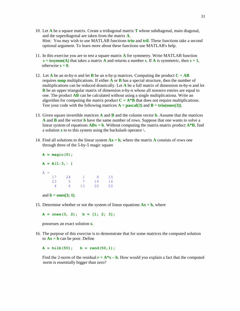
10. Let A be a square matrix. Create a tridiagonal matrix T whose subdiagonal, main diagonal,and the superdiagonal are taken from the matrix A.Hint: You may wish to use MATLAB functions triu and tril . These functions take a secondoptional argument. To learn more about these functions use MATLAB's help.

11. In this exercise you are to test a square matrix A for symmetry. Write MATLAB function s = issymm(A) that takes a matrix A and returns a number s. If A is symmetric, then s = 1, otherwise s = 0.

12. Let A be an m-by-n and let B be an n-by-p matrices. Computing the product C = ABrequires mnp multiplications. If either A or B has a special structure, then the number ofmultiplications can be reduced drastically. Let A be a full matrix of dimension m-by-n and letB be an upper triangular matrix of dimension n-by-n whose all nonzero entries are equal toone. The product AB can be calculated without using a single multiplicationa. Write analgorithm for computing the matrix product C = A*B that does not require multiplications.Test your code with the following matrices A = pascal(3) and B = triu(ones(3)).

13. Given square invertible matrices A and B and the column vector b. Assume that the matricesA and B and the vector b have the same number of rows. Suppose that one wants to solve alinear system of equations ABx = b. Without computing the matrix-matrix product A*B , finda solution x to to this system using the backslash operator \.

14. Find all solutions to the linear system Ax = b, where the matrix A consists of rows onethrough three of the 5-by-5 magic square

A = magic(5);

A = A(1:3,: )

A = 17 24 1 8 15 23 5 7 14 16

4 6 13 20 22

and b = ones(3; 1).

15. Determine whether or not the system of linear equations Ax = b, where

A = ones(3, 2); b = [1; 2; 3];

possesses an exact solution x.

16. The purpose of this exercise is to demonstrate that for some matrices the computed solutionto Ax = b can be poor. Define

A = hilb(50); b = rand(50,1);

Find the 2-norm of the residual r = A*x – b . How would you explain a fact that the computed norm is essentially bigger than zero?

34

17. In this exercise you are to compare computational complexity of two methods for finding asolution to the linear system Ax = b where A is a square matrix. First method utilizes thebackslash operator \ while the second method requires a use of the function rref . UseMATLAB function flops to compare both methods for various linear systems of your choice.Which of these methods require, in general, a smaller number of flops?

18. Repeat an experiment described in Problem 17 using as a measure of efficiency a time needed to compute the solution vector. MATLAB has a pair of functions tic and toc that can be used in this experiment. This illustrates use of the above mentioned functions tic; x = A\b; toc. Using linear systems of your choice compare both methods for speed. Which method is a faster one? Experiment with linear systems having at least ten equations.

19. Let A be a real matrix. Use MATLAB function rref to extract all

(a) columns of A that are linearly independent(b) rows of A that are linearly independent

20. In this exercise you are to use MATLAB function rref to compute the rank of the followingmatrices:

(a) A = magic(3)(b) A = magic(4)(c) A = magic(5)(d) A = magic(6)

Based on the results of your computations what hypotheses would you formulate about the rank(magic(n)), when n is odd, when n is even?

21. Use MATLAB to demonstrate that det(A + B) � det(A) + det(B) for matrices of your choice.

22. Let A = hilb(5). Hilbert matrix is often used to test computer algorithms for reliability. In thisexercise you will use MATLAB function num2str that converts numbers to strings, to seethat contrary to the well-known theorem of Linear Algebra the computed determinantdet(A*A') is not necessarily the same as det(A)*det(A'). You can notice a difference incomputed quantities by executing the following commands: num2str(det(A*A'), 16) andnum2str(det(A)*det(A'), 16).

23. The inverse matrix of a symmetric nonsingular matrix is a symmetric matrix. Check thisproperty using function inv and a symmetric nonsingular matrix of your choice.

24. The following matrix

A = ones(5) + eye(5)

A = 2 1 1 1 1 1 2 1 1 1 1 1 2 1 1 1 1 1 2 1 1 1 1 1 2

35

is a special case of the Pei matrix. Normalize columns of the matrix A so that all columns of the resulting matrix, say B, have the Euclidean norm (2-norm) equal to one.

25. Find the angles between consecutive columns of the matrix B of Problem 24.

26. Find the cross product vector cp that is perpendicular to columns one through four of the Peimatrix of Problem 24.

27. Let L be a linear transformation from �5 to �5 that is represented by the Pei matrix ofProblem 24. Use MATLAB to determine the range and the kernel of this transformation.

28. Let �n denote a space of algebraic polynomials of degree at most n. Transformation Lfrom �n to �3 is defined as follows

=

∫

0

)0(p

dt)t(p

)p(L

1

0

(a) Show that L is a linear transformation.(b) Find a matrix that represents transformation L with respect to the ordered basis {t n, tn –1, … 1}.(c) Use MATLAB to compute bases of the range and the kernel of L . Perform your

experiment for the following values of n = 2, 3, 4.

29. Transformation L from �n to �n –1 is defined as follows L(p) = p'(t) . Symbol �n, isintroduced in Problem 28. Answer questions (a) through (c) of Problem 28 for thetransformation L of this problem.

30. Given vectors a = [1; 2; 3] and b = [-3; 0; 2]. Determine whether or not vector c = [4; 1;1] isin the span of vectors a and b.

31. Determine whether or not the Toeplitz matrix

A = toeplitz( [1 0 1 1 1] )

A = 1 0 1 1 1 0 1 0 1 1 1 0 1 0 1 1 1 0 1 0 1 1 1 0 1

is in the span of matrices B = ones(5) and C = magic(5).

36

32. Write MATLAB function linind(varargin) that takes an arbitrary number of vectors(matrices) of the same dimension and determines whether or not the inputted vectors(matrices) are linearly independent. You may wish to reuse some lines of code that arecontained in the function span presented in Section 3.9 of this tutorial.

33. Use function linind of Problem 32 to show that the columns of the matrix A of Problem31 are linearly independent.

34. Let [a]A = ones(5,1) be the coordinate vector with respect to the basis A – columns of thematrix A of Problem 31. Find the coordinate vector [a]P , where P is the basis of the vectorspace spanned by the columns of the matrix pascal(5).

35. Let A be a real symmetric matrix. Use the well-known fact from linear algebra to determinethe interval containing all the eigenvalues of A. Write MATLAB function

[a, b] = interval(A) that takes a symmetric matrix A and returns the endpoints a and b of the interval that contains all the eigenvalues of A.

36. Without solving the matrix eigenvalue problem find the sum and the product of alleigenvalues of the following matrices:

(a) P = pascal(30)(b) M= magic(40)(c) H = hilb(50)(d) H = hadamard(64)

37. Find a matrix B that is similar to A = magic(3).

38. In this exercise you are to compute a power of the diagonalizable matrix A. Let A = pascal(5). Use the eigenvalue decomposition of A to calculate the ninth power of A. You cannot apply the power operator ^ to the matrix A.

39. Let A be a square matrix. A matrix B is said to be the square root of A if B^2 = A.In MATLAB the square root of a matrix can be found using the power operator ^ . In thisexercise you are to use the eigenvalue-eigenvector decomposition of a matrix find the squareroot of A = [3 3;-2 -2].

40. Declare a variable k to be a symbolic variable typing syms k in the Command Window.Find a value of k for which the following symbolic matrix

A = sym( [1 k^2 2; 1 k -1; 2 –1 0] ) is not invertible.

41. Let the matrix A be the same as in Problem 40.

(a) Without solving the matrix eigenvalue problem, determine a value of k for which all theeigenvalues of A are real.

(b) Let v be a number you found in part (a). Convert the symbolic matrix A to a numericmatrix B using the substitution command subs, i.e., B = subs(A, k, v).

(c) Determine whether or not the matrix B is diagonalizable. If so, find a diagonal matrix Dthat is similar to B.

37

(d) If matrix B is diagonalizable use the results of part (c) to compute all the eigenvectors ofthe matrix B. Do not use MATLAB's function eig.

42. Given a symbolic matrix A = sym( [1 0 k; 2 2 0; 3 3 3]).

(a) Find a nonzero value of k for which all the eigenvalues of A are real.(b) For what value of k two eigenvalues of A are complex and the remaining one is real?